Working paper

The Impact of Peers on Cognitive, Non-cognitive, and Behavioural Outcomes

Evidence from India

Uteeyo Dasgupta Subha Mani Smriti Sharma Saurabh Singhal

July 2015

When citing this paper, please use the title and the following reference number: F-35122-INC-1

! 1!

The Impact of Peers on Cognitive, Non-Cognitive, and Behavioral Outcomes:

Evidence from Indiaa

JULY 2015

PLEASE DO NOT CIRCULATE WITHOUT PERMISSION

UTTEEYO DASGUPTA1, SUBHA MANI2, SMRITI SHARMA3, SAURABH SINGHAL4

Abstract

In this paper, we exploit the variation in the University of Delhi college admission process to estimate the effects of exposure to high achieving peers on cognitive attainment using scores on standardized university level examinations; behavioral outcomes such as risk preference, competitiveness, and confidence; and non-cognitive outcomes using measures of Big Five personality traits. Using a regression discontinuity design, we find that the eligibility to enroll in a better quality college (proxied by peer ability) has a positive effect on cognitive outcomes with larger and more consistent effects for females than males. We also find that exposure to high achieving peers has an effect on selected personality traits and behavioral outcomes. To the best of our knowledge, this is the first paper in the literature to go beyond cognitive outcomes, and also causally identify the effects of exposure to high achieving peers on non-cognitive and behavioral outcomes.

Keywords: Cognitive outcomes, Behavioral outcomes, Personality traits, College

quality, Peer effects, Extra-lab experiments, India

JEL Classification Codes: I23, C9, C14, J24, O15

a Funding was provided by United Nations University-World Institute for Development Economics Research (UNU-WIDER) and International Growth Center – India Central. The funders had no involvement in study design or the collection, analysis, and interpretation of data. 1 Department of Economics, Wagner College, NY, USA, utteeyodasgupta@gmail.com 2 Department of Economics and Center for International Policy Studies, Fordham University, NY, USA; Population Studies Center, University of Pennsylvania, PA, USA; IZA, Bonn, Germany, smani@fordham.edu 3 UNU-WIDER, Helsinki, Finland, smriti@wider.unu.edu 4 UNU-WIDER, Helsinki, Finland, saurabh@wider.unu.edu Acknowledgements: Neha Agarwal, Japneet Kaur, Riju Bafna, Piyush Bhadani, and Anshul Yadav provided excellent research assistance. We are especially grateful to the numerous teachers and principals at the various colleges in the University of Delhi for lending their support in conducting the study. The usual caveat applies.

! 2!

1. Introduction

The returns to college quality have been largely examined using measures of labor

market performance and academic achievement. While most papers find positive and

significant effects of enrollment in elite colleges on wages and employment

outcomes (e.g., Hoekstra, 2009; Saavedra, 2009; Sekhri, 2013), the evidence on the

returns to enrollment in elite colleges on performance in college exit examinations

remains mixed. While Sekhri and Rubinstein (2011), Dale and Krueger (2002),

Black and Smith (2004) and Dale and Krueger (2011) find that better quality

colleges have no value added in terms of college grades, others such as Long (2008),

Saavedra (2009) and Li et al. (2012) find significant benefits.1 While these primarily

focus on the cognitive aspects of human capital, another critical aspect, namely

behavioral preferences and personality traits, often as important in determining labor

market success and well being (Heckman et al., 2006; Lindqvist and Vestman, 2011;

Borghans et. al, 2008; Bowles et al., 2001), have not yet been rigorously examined in

this context.2

The objective of this paper is to close the existing gap in the literature by examining

the returns to exposure to high achieving peers on not just cognitive outcomes, but

also on non-cognitive outcomes that include behavioral preferences and personality

traits. In doing so, we use a regression discontinuity design to address the selection

bias problem arising from the non-random nature of college enrollment (and peer

exposure).

We combine data from a series of unique incentivized extra-lab experiments and

socioeconomic surveys administered to over 2000 undergraduate students at the

University of Delhi (DU), one of the top universities in India, to estimate the effects

of exposure to high achieving peers on three sets of outcomes. The first set of

!!!!!!!!!!!!!!!!!!!!!!!!!!!!!!!!!!!!!!!!!!!!!!!!!!!!!!!!1 Similar conclusions emerge from papers that examine the returns to enrollment in more selective schools on academic performance (Ajayi (2014), Abdulkadiroğlu, Angrist and Pathak (2014), Berkowitz and Hoekstra (2011), Filmer and Schady (2014), Jackson (2010), Lucas and Mbiti (2014), Ozier (2011), and Pop-Eleches and Urquiola (2013)). 2 For instance, Sekhri (2013) due to lack of data that directly measures soft skills, tries to infer this using variables such as reading newspapers, helping others with college work, winning awards etc. which may not be the most appropriate measures of personality traits.

! 3!

outcomes includes measures of cognitive attainment such as scores on standardized

university-level semester examinations. Academic performance and cognitive skills

in general are well-established predictors of labor productivity and earnings (see

Glewwe, 2002 and Hanushek and Woessmann, 2008 for reviews of this literature).

Second, we also examine the effects of exposure to high achieving peers on

behavioral outcomes such as risk preference, competitiveness, and confidence. These

behavioral outcomes have previously been shown to explain important labor market

outcomes. For instance, gender differences in competitiveness have been shown to

explain gender gaps in wages (Niederle and Vesterlund, 2007), job-entry decisions

(Flory et al., 2015), and educational choices (Buser et al., 2014). The level of

confidence also positively affects wages (Fang and Moscarini, 2005) and

entrepreneurial behavior (e.g., Koellinger et al. 2007; Camerer and Lovallo, 1999).

Castillo et al. (2010) find that risk preferences have implications for occupational

sorting.

Finally, we also examine the impact of high achieving peers on Big Five personality

traits. Borghans et al. (2008) document the importance of Big Five conscientiousness

as an important predictor of years of education, grades, and job performance.

Evidence from psychology suggests that personality traits develop through

adolescence and young adulthood with changes in personality being most strong

before one reaches working age (Cobb-Clark and Schurer, 2012, 2013; Specht et al.,

2011). Schurer et al. (2015) estimate the returns to college education on personality

(as measured by Big Five) using Australian data and find substantial variation in the

influence of college enrollment on the Big Five personality traits.

We measure the impact of exposure to peers by using data on enrollment of students

in different colleges of DU that vary in terms of their selectivity as determined by

their admission criterion. Typically, obtaining the causal effect of enrolling in better

quality colleges can be a challenge, as students are not randomly assigned to colleges

and there is significant selection into colleges based on student ability. The

admission criterion for colleges in DU allows us to exploit a regression discontinuity

(RD) design. Students’ report average scores on national high school exit

examinations to apply to colleges and disciplines of their choice in DU and each

! 4!

college then declares discipline-specific cutoffs such that all students with scores

above the cutoff are eligible to take admission in that college-discipline. We exploit

students’ inability to manipulate this admission cutoff and compare students just

above and below the cutoff to determine the impact of their eligibility to enroll in a

better quality college, such that the marginal student to the right of the cutoff is

surrounded by high-achieving peers.

To the best of our knowledge, this is the first paper in the literature to use a RD

design to examine the effects of exposure to college quality on cognitive, behavioral,

and non-cognitive aspects of human capital. Our results indicate that exposure to

high achieving peers leads to gains in scores on standardized university-level

semester examinations, in particular for females. We also find that exposure to these

peers has an effect on risk preferences for females such that females become less

risk-averse. Further, we find that males exposed to high achieving peers are less

likely to be open to experience. We find no significant effect of peer exposure on

other personality traits and behavioral outcomes. We find higher attendance rates

among females to be one of the likely channels explaining the gender differences in

returns to better peer environment. Our results are robust to number of checks

prescribed in the RD design literature.

The rest of the paper is organized as follows. We provide a description of the college

admissions process, sampling strategy, subject recruitment, and data in Section 2.

The empirical specification is outlined in Section 3. The main results are presented in

Section 4 and robustness checks are presented in Section 5. Finally, concluding

comments follow in Section 6.

2. Background and Data

2.1 College Admissions Process

Our sample of interest is 2nd and 3rd year students enrolled in the 3-year

undergraduate degree program in the DU, which includes 79 affiliated colleges with

considerable variation in quality.

In DU, college admission for most disciplines is based solely on an average score

! 5!

computed as the best of four out of five subjects (including language) taken during

the students’ high school exit examination at the end of class 12. Students

simultaneously apply to colleges and disciplines (within those colleges) of their

choice in the month of June each year. Based on capacity constraints and the

incoming cohort’s average score, each discipline within a college then announces the

cutoff scores that determine admission into the specific college and discipline.3 All

those above the cutoff in the discipline are eligible to take admission in the college-

discipline. Since there is greater demand for better quality colleges and they are

oversubscribed, the cutoffs for these colleges are significantly and systematically

higher than the low-quality colleges, usually across several disciplines. If there are

vacancies, the college gradually lowers the cutoff through a number of rounds until

all spots are filled. As expected, the better quality colleges fill their seats within the

first couple of rounds while the lower quality colleges sequentially lower their

cutoffs, taking at times up to 10 such rounds to fill their seats. This real-life

allocation mechanism is equivalent to the Gale and Shapley (1962) college-

proposing mechanism and the resulting matching is stable (for a review, see Sönmez

and Ünver, 2011). This process results in an allocation where typically the high

achieving students attend the better quality colleges while the low achieving students

get admitted to the lower quality colleges. This also results in a discontinuity in the

probability of enrollment into a better quality college at the cutoff. We exploit this

discontinuity in the admission process and compare the cognitive, behavioral, and

personality outcomes of 2nd and 3rd year college students just above the cutoff to

those just below the cutoff to compute the impact of the eligibility to enroll in a

better quality college on these outcomes.

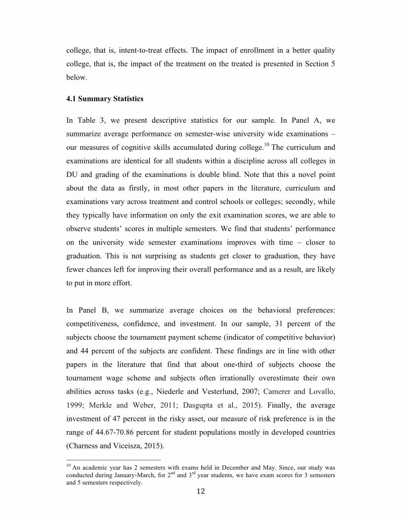
Due to the design of the admissions process in DU, students who are eligible to

enroll in a better quality college are exposed to better quality peers who have

substantially higher average scores on the high school exit examinations compared to

students enrolled in lower quality colleges (See Figure 1).

2.2 Sampling Strategy and Recruitment of Subjects

!!!!!!!!!!!!!!!!!!!!!!!!!!!!!!!!!!!!!!!!!!!!!!!!!!!!!!!!3 These cut-offs are publicly available at http://www.du.ac.in/index.php?id=664

! 6!

We constructed our sample in the following manner. First, to ensure representation

of colleges at both the high and low end of the college quality spectrum, we obtained

the list of all 79 colleges affiliated with DU. Second, we drew a list of 58 colleges

that offer courses in the commerce and arts streams. The 58 colleges that offer

courses in these two streams can be further categorized into: morning coeducational

colleges (31), morning women only colleges (10) and evening colleges (17). We

further restrict ourselves to the coeducational colleges, as they are far more over-

subscribed than the evening and women colleges. Furthermore, the lack of variation

in college cutoffs among the women colleges makes it difficult to obtain a sufficient

number of colleges both above and below the cutoffs. Of the 31 morning colleges,

we further rule out colleges that offer too few courses or use religious criteria or any

criteria other than the average class 12th examination scores for admission purposes,

resulting in a list of 25 target colleges. After considering admission cutoffs for each

of these 25 colleges for three consecutive years (2011-13), we identified 18 colleges

that had consistently ranked admission cutoffs across the three years for the two

disciplines of economics and commerce. These two disciplines are the most popular

and competitive disciplines and have significantly higher levels of enrollment

compared to other disciplines. We targeted 17 of these identified colleges, of which

we were able to implement our study in 15 colleges with varying cutoffs. We

conducted the study with 2065 2nd and 3rd year students in these 15 colleges during

January-March 2014 in regular class hours, in coordination with the respective

teachers.

2.3 Extra-lab Experiments and Survey

In the first part of the study, we conducted incentivized extra-lab experiments to

obtain measures of behavioral outcomes. 4 First, to capture subjects’ competitiveness

and confidence we used a simple number-addition task (similar to Niederle and

Vesterlund, 2007). After a practice session, participants had to predict their

performances in advance, and also choose between a piece-rate and tournament

compensation scheme. Under the piece-rate scheme, Rs. 10 was paid for every

correct answer. Under the tournament scheme, Rs. 20 was paid for every correct

!!!!!!!!!!!!!!!!!!!!!!!!!!!!!!!!!!!!!!!!!!!!!!!!!!!!!!!!4 Subject instructions for the experimental module are available from the authors upon request.

! 7!

answer if the subject out-performed a randomly selected student of DU who had

solved the questions earlier.5 We define competitiveness as a dummy that takes a

value 1 if the subject chose the tournament compensation scheme and 0 if the subject

chose the piece-rate compensation scheme. We define confidence as a dummy that

takes a value 1 if the subject believes that her performance in the actual task will

exceed those of others in the same session, 0 otherwise.

Second, to measure risk preferences, we used the investment game of Gneezy and

Potters (1997). In this, subjects allocated a portion of their endowment (Rs. 150) to a

risky lottery and set aside the remainder. If they won the lottery based on a roll of a

dice, the invested amount would be tripled and they would also get any amount they

set aside. Conversely, if they lost the lottery, they would only receive the amount

that was set aside. We define investment as the proportion allocated to the risky

lottery in the investment game.

In the second part of the study, we implemented a socioeconomic survey that

collected details on family background characteristics, school and college

information, academic performance, aspirations, and details on participation in extra-

curricular activities. To measure cognitive outcomes, we collected data on scores on

semester-wise university examinations. To measure personality traits, we

administered the 10-item Big-Five inventory (Gosling et al., 2003). The five traits in

the Big Five are defined as follows. Openness to experience is the tendency to be

open to new aesthetic, cultural, or intellectual experiences. Conscientiousness refers

to a tendency to be organized, responsible, and hard working. Extraversion relates to

an outward orientation rather than being reserved. Agreeableness is related to the

tendency to act in a cooperative and unselfish manner. Neuroticism (opposite of

Emotional stability) is the tendency to experience unpleasant emotions easily, such

as anger, anxiety, depression, or vulnerability.

Overall, we conducted 60 sessions with 2065 subjects, resulting in approximately 34

subjects per session. Each session lasted about 75 minutes. All subjects received a

!!!!!!!!!!!!!!!!!!!!!!!!!!!!!!!!!!!!!!!!!!!!!!!!!!!!!!!!5 Following Bartling et al. (2009), we implemented a pilot version of this game where 40 students from DU had participated in this game. We use the performance of these students for comparison in the tournament wage scheme.

! 8!

show-up fee of Rs. 150. Further, in each session, 20 percent of the subjects were

randomly chosen to be paid for their decisions on one of the randomly chosen tasks

from the experiment module. The average additional payment was Rs. 230. All

subjects participated only once in the study.

3. Empirical Specification

For the purpose of this analysis, we exclude all those students who were not admitted

on the basis of discipline-specific cutoffs. This includes students belonging to

disadvantaged backgrounds (Scheduled Castes, Scheduled Tribes and Other

Backward Castes) for whom affirmative action policies mandate a fixed number of

seats; students admitted on the basis of excellence in sports or other extra-curricular

activities, those who transferred from one college to another after enrollment or

switched disciplines within a college; and those providing insufficient identification

information.6 This reduces our sample to 1329 subjects. We follow the procedure

outlined in Pop-Eleches and Urquiola (2013) to construct our final sample from the

pool of 1329 eligible subjects. We use admission cutoffs as exogenously announced

by the individual colleges as our criteria to sort the 15 colleges in our sample into the

following four categories such that the group of colleges that belong to the higher

categories have consistently higher admission cutoffs than the cutoffs of the groups

of colleges that belong to the lower categories. The 15 colleges in our sample are

consequently given four ranks ranging from 1 (lowest rank) to 4 (highest rank).

Since cutoffs also vary by discipline (commerce and economics), combination of

subjects in high school, gender and year, for each rank, we use three sets of cutoffs

for our four ranks, where each rank (and colleges therein) receives a cutoff equal to

the lowest admission cutoff released by the higher ranked college in that category.

Note that in each rank, the cutoffs also vary by discipline, gender, and year. So the

rank 4 colleges receive a cutoff equal to the lowest admission cutoff released by this

group of colleges and results in an RD sample where colleges in rank 4 are assigned

to the treatment (better quality college) and the remaining colleges (in ranks 3, 2, and

1) are assigned to be the control (lower quality college). Next, colleges in ranks 3

!!!!!!!!!!!!!!!!!!!!!!!!!!!!!!!!!!!!!!!!!!!!!!!!!!!!!!!!6 Of 2065 students in our sample, 29 percent are affirmative action beneficiaries, 4.8 percent got admitted on the basis of sports and other activities, 0.6 percent migrated within or across colleges and 1.4 percent provided insufficient information.

! 9!

and 4 would receive a cutoff equal to the lowest admission cutoff released by this

group of colleges and results in an RD sample where colleges ranked 3 and 4 are

assigned to the treatment and the remaining colleges (ranks 2 and 1) are assigned to

the control. Finally, a third sample is constructed where colleges ranked 4, 3, and 2

receive a cutoff equal to the lowest admission cutoff released by this group of

colleges and results in an RD sample where these colleges are assigned to the

treatment group and colleges in rank 1 are assigned to the control. We finally “stack”

all three sets of between college rank cutoffs that also vary by discipline, gender, and

year to create our final analysis sample that now includes 3656 subjects.

We estimate the following “intent-to-treat” type OLS regression model using a RD

approach:

!! = !! + !!!! + !!!! + !!!!! + !!!!!! + !!!!!!! + !!X!" +!!!!! !! !!!!!!!!!!!!!!!!(1)

Where Yi is the outcome variable, di is the running variable computed as the

difference between student i’s average class 12 examination score and the relevant

college rank-discipline-year specific cutoff, Ti takes a value 1 if di is non-negative

and 0 otherwise. We control for the running variable to account for selection on

observables (Heckman and Robb, 1985). Further, we also allow for a quadratic

specification in the running variable to allow for non-linearity in the relationship

between the outcome and the running variable.7 We also include a vector of

controls/pre-determined characteristics (Xs) such as mother's education, father's

education, number of siblings, private school enrollment, age, family income, and

religion to improve the precision of our estimates. Finally, !! is the iid error term. All

regression estimates are clustered at the session level. In this specification, !!

captures the intent-to-treat effect or the effect of being eligible to enroll in a better

quality college or exposure to better quality peers at the cutoff.

Note, not all students eligible to enroll in the better quality college (treatment) will

take admission in that college. Similarly, some students assigned to the low quality

!!!!!!!!!!!!!!!!!!!!!!!!!!!!!!!!!!!!!!!!!!!!!!!!!!!!!!!!7 In the robustness section, we also present the effects using alternative parametric models. Overall, we do not find our results susceptible to the parameterization of the control function, the sample size and or the estimation technique employed (OLS, IV).

! 10!

colleges might seek admission into the higher quality college through personal

connections with the principal, for instance.8 Imperfect compliance entails the

application of a “fuzzy” RD design (Hahn, Todd and Van der Klaauw 2001; Lee and

Lemieux 2010) where the treated (TRi), i.e., enrolled in a better quality college will

be instrumented by the discontinuity in the running variable. The corresponding first-

stage regression would be:

!"! = !! + !!!! + !!!! + !!!!! + !!!!!! + !!!!!!! + !!X!" +!!!!! !! !!!!!!!!!!!!!!!!!!!!!!!!!!!!!!!(2)

and the corresponding second-stage regression would be:

!! = !! + !!!"! + !!!! + !!!!! + !!!!!! + !!!!!!! + !!X!" +!!!!! !! !!!!!!!!!!!!!!!!!!!!!!!!!!!!!!!!!(3)

Where the coefficient estimate on TR gives us the local average treatment effect

(LATE) from being enrolled in a better quality college, computed as the ratio of the

reduced form coefficients (!! = !!/!!) as long as we use the same bandwidth and

polynomial order as in equations (1) - (3).

3.1 Testing the validity of the RD design

The “fuzzy” RD model relies on two assumptions: (a) there is no manipulation of the

assignment variable at the cutoff, and (b) the probability of being enrolled in a better

quality college is discontinuous at the cutoff. This is also proof of a strong first-stage

regression, necessary for obtaining a valid second stage estimate.

The estimation strategy would result in biased estimates if students could perfectly

control the side of the cutoff they will fall under. However, as we argue below, this

is not possible under the admission process in DU. First, the scoring of the class 12

examinations is double blind, making manipulation of the scores difficult, if not

outright impossible. Second, at the time of application to DU colleges, students do

not know what the various cutoffs will be for that year.9 Moreover, since the rule for

!!!!!!!!!!!!!!!!!!!!!!!!!!!!!!!!!!!!!!!!!!!!!!!!!!!!!!!!8 In our sample, only 0.67 percent of the subjects who have a negative distance from the cutoff are enrolled in a higher ranked college and approximately 12 percent of the subjects who have a positive distance from the cutoff are enrolled in a lower ranked college. 9 Based on historical trends, students may have a rough sense of the range of the cutoff, but this does not invalidate our analysis.

! 11!

determining these cutoffs is never public knowledge, students cannot perfectly

predict future cutoffs. Overall, it is virtually impossible for students to perfectly

manipulate either the class 12 examination scores or the side of the college cutoff

they will ultimately fall on.

As colleges are required to simultaneously reduce cutoffs till there are no vacancies,

it is very unlikely that students just above the cutoff differ systematically from those

just below the cutoff on unobservables. We can, however, check for discontinuities

in other predetermined characteristics. To do this, we collected information on

family background characteristics such as mother's education, father's education,

number of siblings, private school enrollment, age, family income, and religion. In

Table 1 we formally test for discontinuity in each of these covariates by estimating

equation (1) with the predetermined family background characteristics as the

dependent variables. Since our main impact estimates are presented for the pooled

sample, and separately by gender, we examine the validity of the RD design in Table

1 separately for the pooled sample (Panel A), males (Panel B), and females (Panel

C). We find that the impact of the treatment indicator on the predetermined variables

is mostly small and never significantly different from zero, confirming the validity of

the RD design.

In Table 2 below, we present estimates from equation (2). We find that students who

are eligible to enroll in a better quality college are 75 percent more likely to do so.

We find similar strong effects of the eligibility to enroll in a better quality college for

both males and females. We find that the admission rules used in DU are therefore

strong with some imperfect compliance making the fuzzy RD design appropriate to

follow. The results from the corresponding IV specification are presented in the

Robustness section. We also present the first-stage relationship between enrollment

in a better quality college and the running variable for the pooled sample, males, and

females in Figure 2. We see a clear jump in the probability of enrolling in a better

quality college at the cutoff for all three samples in Figure 2.

4. Results

Our primary results focus on the impact of being eligible to enroll in a better quality

! 12!

college, that is, intent-to-treat effects. The impact of enrollment in a better quality

college, that is, the impact of the treatment on the treated is presented in Section 5

below.

4.1 Summary Statistics

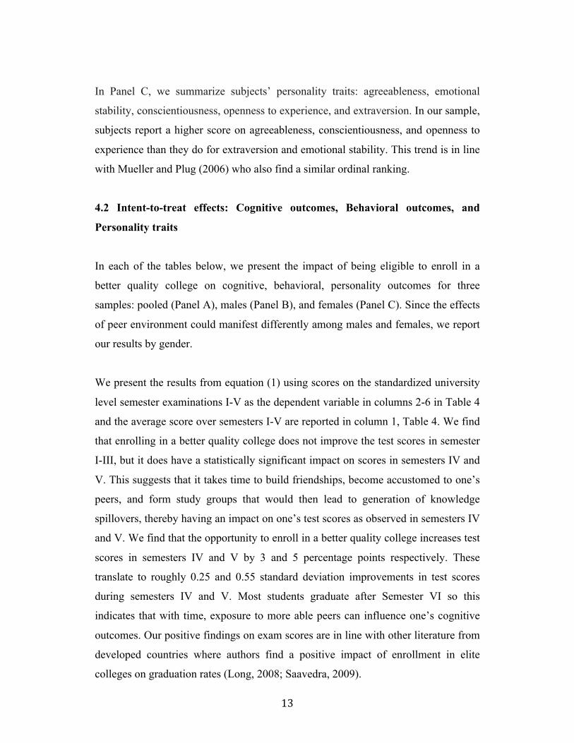
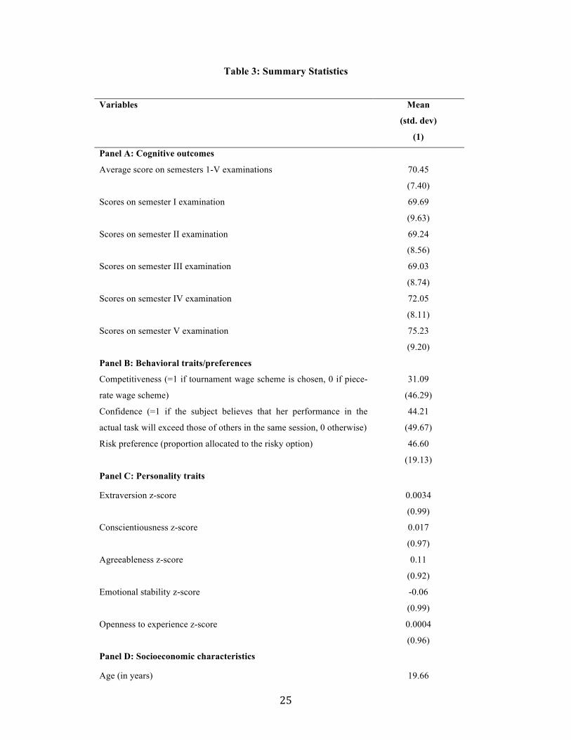
In Table 3, we present descriptive statistics for our sample. In Panel A, we

summarize average performance on semester-wise university wide examinations –

our measures of cognitive skills accumulated during college.10 The curriculum and

examinations are identical for all students within a discipline across all colleges in

DU and grading of the examinations is double blind. Note that this a novel point

about the data as firstly, in most other papers in the literature, curriculum and

examinations vary across treatment and control schools or colleges; secondly, while

they typically have information on only the exit examination scores, we are able to

observe students’ scores in multiple semesters. We find that students’ performance

on the university wide semester examinations improves with time – closer to

graduation. This is not surprising as students get closer to graduation, they have

fewer chances left for improving their overall performance and as a result, are likely

to put in more effort.

In Panel B, we summarize average choices on the behavioral preferences:

competitiveness, confidence, and investment. In our sample, 31 percent of the

subjects choose the tournament payment scheme (indicator of competitive behavior)

and 44 percent of the subjects are confident. These findings are in line with other

papers in the literature that find that about one-third of subjects choose the

tournament wage scheme and subjects often irrationally overestimate their own

abilities across tasks (e.g., Niederle and Vesterlund, 2007; Camerer and Lovallo,

1999; Merkle and Weber, 2011; Dasgupta et al., 2015). Finally, the average

investment of 47 percent in the risky asset, our measure of risk preference is in the

range of 44.67-70.86 percent for student populations mostly in developed countries

(Charness and Viceisza, 2015).

!!!!!!!!!!!!!!!!!!!!!!!!!!!!!!!!!!!!!!!!!!!!!!!!!!!!!!!!10 An academic year has 2 semesters with exams held in December and May. Since, our study was conducted during January-March, for 2nd and 3rd year students, we have exam scores for 3 semesters and 5 semesters respectively.

! 13!

In Panel C, we summarize subjects’ personality traits: agreeableness, emotional

stability, conscientiousness, openness to experience, and extraversion. In our sample,

subjects report a higher score on agreeableness, conscientiousness, and openness to

experience than they do for extraversion and emotional stability. This trend is in line

with Mueller and Plug (2006) who also find a similar ordinal ranking.

4.2 Intent-to-treat effects: Cognitive outcomes, Behavioral outcomes, and

Personality traits

In each of the tables below, we present the impact of being eligible to enroll in a

better quality college on cognitive, behavioral, personality outcomes for three

samples: pooled (Panel A), males (Panel B), and females (Panel C). Since the effects

of peer environment could manifest differently among males and females, we report

our results by gender.

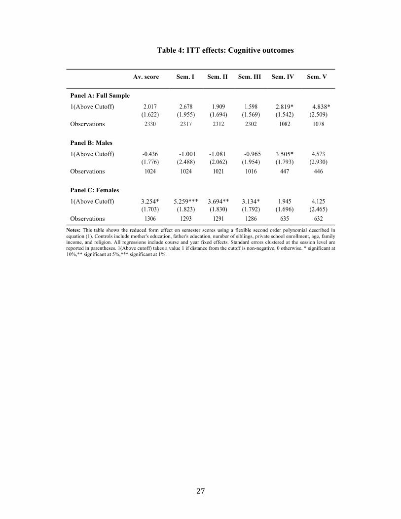
We present the results from equation (1) using scores on the standardized university

level semester examinations I-V as the dependent variable in columns 2-6 in Table 4

and the average score over semesters I-V are reported in column 1, Table 4. We find

that enrolling in a better quality college does not improve the test scores in semester

I-III, but it does have a statistically significant impact on scores in semesters IV and

V. This suggests that it takes time to build friendships, become accustomed to one’s

peers, and form study groups that would then lead to generation of knowledge

spillovers, thereby having an impact on one’s test scores as observed in semesters IV

and V. We find that the opportunity to enroll in a better quality college increases test

scores in semesters IV and V by 3 and 5 percentage points respectively. These

translate to roughly 0.25 and 0.55 standard deviation improvements in test scores

during semesters IV and V. Most students graduate after Semester VI so this

indicates that with time, exposure to more able peers can influence one’s cognitive

outcomes. Our positive findings on exam scores are in line with other literature from

developed countries where authors find a positive impact of enrollment in elite

colleges on graduation rates (Long, 2008; Saavedra, 2009).

! 14!

Upon further examining these effects by gender, we find that it is females who

benefit from the exposure to better peers, and these effects peter out over time.

Our findings suggest that students just above the cutoff (are students with relatively

low-ability when compared to their peers) benefit from being exposed to their higher

ability peers compared to students just below the cutoff (who are of high-ability

compared to their peers in the lower quality college). Our main result is consistent

with Jain and Kapoor (2015) who find that it is low-ability students when randomly

assigned to high-ability peers that benefit compared to high-ability students using

data on students’ academic performance in a prestigious business school in India.

The second set of results concern behavioral outcomes – competitiveness,

confidence, and investment. The ITT effects for these traits are shown in Table 5

below. While in the pooled sample and among males, we do not find any significant

effects, we find that females differ significantly in their risk preferences. Our results

indicate that women who are eligible to enroll in better quality college invest almost

7 percentage points more in the investment game, therefore being less risk-averse

than their female counterparts not eligible to enroll in the better quality college. To

the extent that females are more risk-averse than males and this gender gap in risk

preferences has implications for selecting into competitive environments and

occupational choice, this result suggests that higher quality colleges may result in a

narrowing of this gender gap.

The last set of impact estimates pertains to personality outcomes – Big Five traits of

openness to experience, conscientiousness, extraversion, agreeableness and

emotional stability (Table 6). We find no impact of eligibility to enroll in a higher

quality college on most Big Five traits except openness to experience that reduces by

0.21 standard deviations. Further upon splitting the data by gender, we find that this

decline in openness to experience occurs only for males (by 0.365 standard

deviations). Overall, our results suggest that knowledge is more transferable and

! 15!

hence can influence examination scores more easily than personality traits that are

less malleable through the channel of ‘direct tutoring’.

We explore the potential pathways for these gender differential results in Table 10

and find higher attendance rates among females to be one of the likely channels

explaining the gender differences in returns to better peer environment.

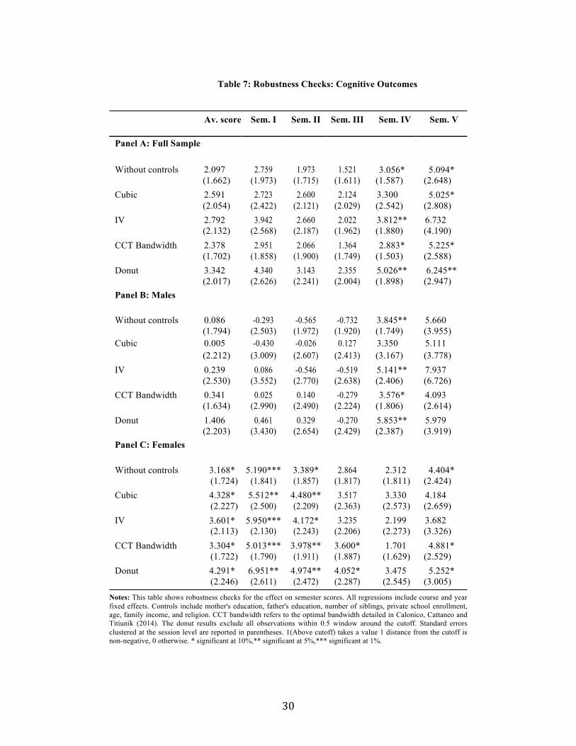
5. Robustness

We show here that the intent-to-treat effects reported earlier in Tables 4-6 are robust

to a number of econometric concerns such as: choice of the polynomial order,

bandwidth selection, estimation technique, and measurement error around the cutoff.

Robustness results are presented for pooled sample, males and females in Tables 7-9.

First, to check for specification bias arising from the choice of second order

polynomial, we present the impact of eligibility to enroll in a better quality college

on all outcomes using a flexible cubic polynomial and find that the results remain

largely similar to the ones presented earlier in Tables 4-6.

Second, we also present the estimates from the IV strategy described previously in

Section 3. We find that our IV or LATE results are consistently higher than the OLS

estimates reported in Tables 4-6.

Third, we restrict our data to the optimal bandwidth prescribed by Calonico,

Cattaneo and Titiunik (2014) and find our results to be robust to the width of the

window around the cutoff.

Finally, it has been argued that if there is manipulation, it is likely to occur right

around the cutoff. One way to check if the results are robust to such possible

behavior is to discard the observations near the cutoff and re-estimate the model

(Barreca et al., 2011; Filmer and Schady, 2014). We report results from these

“donut” regressions where we exclude all observations within (-0.5, 0.5) window

around the cutoff and re-estimate equation (1) and once again, find that our primary

results continue to hold.

! 16!

6. Discussion and Conclusion

To the best of our knowledge, this is the first paper in the literature that goes beyond

previously examined cognitive outcomes to causally identify the effects of exposure

to better peers - as captured by college selectivity - on cognitive, behavioral, and

personality outcomes. We exploit the variation in college admission cutoffs along

and compare students just above the cutoff with those just below the cutoff to

determine the impact of the eligibility to enroll in a better quality college, where they

are exposed to relatively high-achieving peers, on these outcomes.

Using data from 2nd and 3rd year college students enrolled in commerce and

economics disciplines, our results indicate that the exposure to a superior peer

environment improves scores on standardized semester exams, particularly for

females. In terms of behavioral and personality traits, we find that females with

access to better quality colleges are less risk-averse, while males in these colleges are

less likely to be open to experiences. However, we do not observe significant effects

on other traits.

While we are able to estimate the returns to college quality for a range of new

outcomes considered important in the literature, it should be noted that we are not

able to examine these effects for the entire population of DU students. Also, since

DU is one of the premier universities in India, its students are not representative of

the average Indian college student. Our results must be assessed keeping these

limitations in mind.

! 17!

References

Ajayi, K.F. (2014). Does School Quality Improve Student Performance? New Evidence from Ghana. Working Paper. Abdulkadiroğlu, A., Angrist, J.D., and Pathak, P.A. (2014). The Elite Illusion: Achievement Effects at Boston and New York Exam Schools. Econometrica, 82(1), 137-196. Barreca, A. I., Guldi, M., Lindo, J. M., and Waddell, G. R. (2011). Saving babies? Revisiting the effect of very low birth weight classification. Quarterly Journal of Economics, 126(4), 2117-2123. Bartling, B., Fehr, E., Maréchal, M.A., and Schunk, D. (2009). Egalitarianism and Competitiveness. American Economic Review: Papers & Proceedings 2009, 99(2), 93-98. Berkowitz, D., and Hoekstra, M. (2011). Does high school quality matter? Evidence from admissions data. Economics of Education Review, 30, 280-288. Black, D.A. and Smith, J.A. (2004). How robust is the evidence on the effects of college quality? Evidence from matching. Journal of Econometrics, 121, 99-124.

Borghans, L., Duckworth, A.L., Heckman, J.J., and ter Weel, B. (2008). The Economics and Psychology of Personality Traits. Journal of Human Resources, 43(4), 972-1059.

Bowles, S., H. Gintis, and M. Osborne. 2001. "The Determinants of Earnings: A Behavioral Approach." Journal of Economic Literature, 39(4): 1137-1176.

Buser, T., M. Niederle and H. Oosterbeek (2014). Gender, Competitiveness and Career Choices. Quarterly Journal of Economics, doi: 10.1093/qje/qju009.

Calonico, S., Cattaneo, M. D., and Titiunik, R. (2014). Robust Nonparametric Confidence Intervals for Regression-Discontinuity Designs. Econometrica, 82(6), 2295-2326.

Camerer, C. F. and D. Lovallo (1999). Overconfidence and Excess Entry: An Experimental Approach. American Economic Review, 89, 306 - 318.

Castillo, M., Petrie, R. and Torero, M. (2010). On the Preferences of Principals and Agents. Economic Inquiry, 48(2), 266 - 273.

Charness, G., and Viceisza, A. (2015). Three risk elicitation methods in the field: evidence from rural Senegal. Working Paper Cobb-Clark, D.A., and Schurer, S. (2012). The stability of big five personality traits. Economics Letters, 115, 11-15.

Cobb-Clark, D.A., and Schurer, S. (2013). Two economists’ musings on the stability

! 18!

of locus of control. The Economic Journal, 123 F358-F400.

Dale, S., and Krueger, A.B. (2002). Estimating the Payoff to Attending a More Selective College: An Application of Selection on Observables and Unobservables. Quarterly Journal of Economics, 117(4), 1491–1527

Dale, S., and Krueger, A.B. (2011). Estimating the return to college selectivity over the career using administrative earning data. IZA Discussion Paper No. 5533.

Dasgupta, U., Gangadharan, L., Maitra, P., Mani, S., and Subramanian, S. (2015). Choosing to be Trained: Do Behavioral Traits Matter? Journal of Economic Behavior and Organization, 110, 145-159

Fang, H. and G. Moscarini (2005). Morale Hazard. Journal of Monetary Economics, 52(4), 749-777.

Filmer, D., and Schady, N. (2014). The Medium- Term Effects of Scholarships in a Low- Income Country. Journal of Human Resources, 49(3), 663-694. Flory, J. A., Leibbrandt, A., and List, J. A. (2015). Do competitive work places deter female workers? A large-scale natural field experiment on job entry decisions. Review of Economic Studies, 82(1), 122-155.

Gale, D., and Shapley, L.S. (1962). College admissions and the stability of marriage. American Mathematical Monthly, 69 (1), 9-15.

Glewwe, P. (2002). Schools and skills in developing countries: education policies and socioeconomic outcomes. Journal of Economic Literature, 40(2), 436-482.

Gneezy, U. and Potters, J. (1997). An experiment on risk taking and evaluation periods. Quarterly Journal of Economics, 112(2), 631-645

Gosling, S.D., Rentfrow, P.J., and Swann Jr., W.B. (2003). A very brief measure of the Big-Five personality domains. Journal of Research in Personality, 37, 504-528.

Hanushek, E., and Woessmann, L. (2008). The role of cognitive skills in economic development. Journal of Economic Literature, 46(3), 607-668

Hahn, J., Todd, P., and Van der Klaauw, W. (2001). Identification and estimation of treatment effects with a regression-discontinuity design. Econometrica, 69(1), 201-209.

Heckman, J., and Robb, R. Jr. (1985). Alternative Methods for Evaluating the Impact of Interventions: An Overview. Journal of Econometrics, 30 (1-2): 239-267.

Heckman, J.J., Stixrud, J., Urzúa, S. (2006). The effects of cognitive and non-cognitive abilities on labor market outcomes and social behavior. Journal of Labor Economics, 24(3), 411–482

Hoekstra, M. (2009). The effect of attending the flagship state university on

! 19!

earnings: a discontinuity-based approach. Review of Economics and Statistics, 91(4), 717-724.

Jain, T., and Kapoor, M. (2015). The impact of study groups and roommates on academic performance. Review of Economics and Statistics, 97(1), 44-54.

Jackson, C. K. (2010). Do Students Benefit from Attending Better Schools? Evidence from Rule-based Student Assignments in Trinidad and Tobago. Economic Journal, 120(549), 1399–1429. Koellinger, P., M. Minniti and C. Schade (2007). ‘I think I can, I think I can’: Overconfidence and Entrepreneurial Behavior. Journal of Economic Psychology, 28, 502 - 527. Lee, D. S., and Lemieux, T. (2010). Regression Discontinuity Designs in Economics. Journal of Economic Literature, 48(2), 281–355. Li, H., Meng, L., Shi, X., and Wu, B. (2012). Does attending elite colleges pay in China? Journal of Comparative Economics, 40, 78-88. Lindqvist, E. and Vestman, R. (2011). The Labor Market Returns to Cognitive and Noncognitive Ability: Evidence from the Swedish Enlistment. American Economic Journal: Applied Economics, 3(1), 101-128. Long, M. (2008). College quality and early adult outcomes. Economics of Education Review, 27, 588–602

Lucas, A.M., and Mbiti, I.M. (2014). Effects of School Quality on Student Achievement: Discontinuity Evidence from Kenya. American Economic Journal: Applied Economics, 6(3), 234-263 Merkle, C., and Weber, M. (2011). True overconfidence: The inability of rational information processing to account for apparent overconfidence. Organizational Behavior and Human Decision Processes, 116(2), 262-271.

Mueller, G., and Plug, E. (2006). Estimating the effects of personality on male and female earnings. Industrial and Labor Relations Review, 60 (1), 3–22. Niederle, M. and Vesterlund, L. (2007). Do Women Shy Away from Competition? Do Men Compete to Much? Quarterly Journal of Economics, 122(3), 1067–1101. Ozier, O. (2011). The Impact of Secondary Schooling in Kenya: A Regression Discontinuity Analysis. Working Paper. Pop-Eleches, C., and Urquiola, M. (2013). Going to a Better School: Effects and Behavioral Responses. American Economic Review, 103(4), 1289-1324. Saavedra, J. (2009). The learning and early labor market effects of college quality: a regression discontinuity analysis. Working paper.

! 20!

Schurer, S., Kassenboehmer, S.C., and Leung, F. (2015). Do universities shape their students’ personality. IZA DP No. 8873

Sekhri, S. (2013). Prestige matters: Value of connections formed in elite colleges. IGC working paper.

Sekhri, S., and Y. Rubinstein (2011). Public Private College Educational Gap in Developing Countries: Evidence on Value Added versus Sorting from General Education Sector in India. Working paper.

Sönmez, T., and M. U. Ünver (2011). Matching, Allocation and Exchange of Discrete Resources, in J. Benhabib, A. Bisin, and M. Jackson (eds.) Handbook of Social Economics Vol. 1A, Elsevier.

Specht, J., Egloff, B., and Schmukle, S.C. (2011). Stability and change of personality across the life course: the impact of age and major life events on mean-level and rank-order stability of the Big Five. Journal of Personality and Social Psychology, 101(4), 862-882.

! 21!

Figure 1: Difference in Peer Quality

! 22!

Figure 2: First Stage Relationship

! 23!

Table 1: Balance in Baseline Covariates

Age

Mother’s education

Father’s education

No. of Siblings

Hindu

Private School

Family Income

Panel A: Full Sample

1(Above cutoff) 0.036 0.034 -0.033 -0.016 -0.035 0.038 0.023 (0.101) (0.053) (0.051) (0.119) (0.031) (0.051) (0.070)

Observations 2352 2377 2377 2377 2377 2377 2377

Panel B: Males 1(Above Cutoff) 0.025 -0.035 -0.079 -0.198 -0.030 0.009 0.081 (0.200) (0.096) (0.097) (0.210) (0.050) (0.083) (0.096)

Observations 1037 1053 1053 1053 1053 1053 1053 Panel C: Females 1(Above cutoff) 0.088 0.083 -0.013 0.122 -0.054 0.057 -0.043

(0.095) (0.076) (0.061) (0.114) (0.043) (0.062) (0.088) Observations 1315 1324 1324 1324 1324 1324 1324

Notes: This table reports the reduced form estimates using the flexible second order polynomial described in equation (1). All regressions include course and year fixed effects. Standard errors clustered at the session level are reported in parentheses. * significant at 10%,** significant at 5%,*** significant at 1%. 1(Above cutoff) takes a value 1 if distance from the cutoff is non-negative, 0 otherwise.

! 24!

Table 2: First Stage Discontinuity Full Sample Males Females

Without controls 0.748*** 0.730*** 0.758*** (0.057) (0.063) (0.074)

With controls 0.747*** 0.733*** 0.762*** (0.055) (0.063) (0.071)

Observations 2352 1037 1315

Notes: This table shows the first stage discontinuity results using a flexible second order polynomial described in the text. Controls include mother's education, father's education, number of siblings, private school enrollment, age, family income, and religion. All regressions include course and year fixed effects. Standard errors clustered at the session level are reported in parentheses. * significant at 10%,** significant at 5%,*** significant at 1%.

! 25!

Table 3: Summary Statistics

Variables Mean

(std. dev)

(1)

Panel A: Cognitive outcomes

Average score on semesters 1-V examinations

70.45

(7.40)

Scores on semester I examination 69.69

(9.63)

Scores on semester II examination 69.24

(8.56)

Scores on semester III examination 69.03

(8.74)

Scores on semester IV examination 72.05

(8.11)

Scores on semester V examination 75.23

(9.20)

Panel B: Behavioral traits/preferences

Competitiveness (=1 if tournament wage scheme is chosen, 0 if piece-

rate wage scheme)

31.09

(46.29)

Confidence (=1 if the subject believes that her performance in the

actual task will exceed those of others in the same session, 0 otherwise)

44.21

(49.67)

Risk preference (proportion allocated to the risky option) 46.60

(19.13)

Panel C: Personality traits

Extraversion z-score 0.0034

(0.99)

Conscientiousness z-score 0.017

(0.97)

Agreeableness z-score 0.11

(0.92)

Emotional stability z-score -0.06

(0.99)

Openness to experience z-score 0.0004

(0.96)

Panel D: Socioeconomic characteristics

Age (in years) 19.66

! 26!

(0.86)

Male (=1 if male, 0 if female) (in %) 44.13

(49.66)

Hindu (=1 if religious category is Hindu, 0 otherwise) (in %) 92.13

(26.93)

Number of siblings 1.35

(0.72)

Private school (=1 if graduated high school from a private school, 0

otherwise) (in %)

84.81

(35.89)

Mother’s education (=1 if mother has an undergraduate and or higher

degree, 0 otherwise) (in %)

75.30

(43.13)

Father’s education (=1 if father has an undergraduate and or higher

degree, 0 otherwise) (in %)

78.20

(41.29)

Income (=1 if monthly family income <=50,000 Rupee, 0 otherwise)

(in %)

30.54

(46.06)

Notes: Standard deviations are reported in parenthesis. All measures reported in z-scores are standardized using the mean and standard deviation of the control group/lower quality college as the reference category. Sample restricted to +/- 5 window.

! 27!

Table 4: ITT effects: Cognitive outcomes Av. score Sem. I Sem. II Sem. III Sem. IV Sem. V

Panel A: Full Sample

1(Above Cutoff) 2.017 2.678 1.909 1.598 2.819* 4.838* (1.622) (1.955) (1.694) (1.569) (1.542) (2.509)

Observations 2330 2317 2312 2302 1082 1078

Panel B: Males

1(Above Cutoff) -0.436 -1.001 -1.081 -0.965 3.505* 4.573 (1.776) (2.488) (2.062) (1.954) (1.793) (2.930)

Observations 1024 1024 1021 1016 447 446

Panel C: Females

1(Above Cutoff) 3.254* 5.259*** 3.694** 3.134* 1.945 4.125 (1.703) (1.823) (1.830) (1.792) (1.696) (2.465)

Observations 1306 1293 1291 1286 635 632 Notes: This table shows the reduced form effect on semester scores using a flexible second order polynomial described in equation (1). Controls include mother's education, father's education, number of siblings, private school enrollment, age, family income, and religion. All regressions include course and year fixed effects. Standard errors clustered at the session level are reported in parentheses. 1(Above cutoff) takes a value 1 if distance from the cutoff is non-negative, 0 otherwise. * significant at 10%,** significant at 5%,*** significant at 1%.

! 28!

Table 5: ITT effects: Behavioral outcomes Competition Confidence Investment

Panel A: Full Sample 1(Above Cutoff) 0.059 -0.061 2.114

(0.064) (0.063) (2.210) Observations 2349 2352 2343

Panel B: Males 1(Above Cutoff) 0.082 0.080 -1.965

(0.086) (0.101) (4.216) Observations 1037 1037 1032

Panel C: Females

1(Above Cutoff) 0.100 -0.087 7.748*** (0.072) (0.077) (2.691)

Observations 1312 1315 1311 Notes: This table shows the reduced form effect on behavioral outcomes using a flexible second order polynomial described in equation (1). Controls include mother's education, father's education, number of siblings, private school enrollment, age, family income, and religion. All regressions include course and year fixed effects. Standard errors clustered at the session level are reported in parentheses. 1(Above cutoff) takes a value 1 if distance from the cutoff is non-negative, 0 otherwise. * significant at 10%,** significant at 5%,*** significant at 1%.

! 29!

Table 6: ITT effects: Personality Traits

Big Five Extraversion Agreeableness Conscientiousness Emotional Openness to Stability experience

Panel A: Full Sample 1(Above Cutoff) -0.166 0.162 -0.103 0.012 -0.220*

(0.123) (0.103) (0.128) (0.108) (0.114) Observations 2315 2302 2324 2313 2312 Panel B: Males 1(Above Cutoff) -0.181 0.116 -0.271 0.064 -0.372**

(0.174) (0.218) (0.172) (0.169) (0.186) Observations 1015 1007 1023 1012 1012 Panel C: Females 1(Above Cutoff) -0.159 0.124 0.053 -0.050 -0.049

(0.175) (0.111) (0.196) (0.174) (0.147) Observations 1300 1295 1301 1301 1300

Notes: This table shows the reduced form effect on personality traits using a flexible second order polynomial described in equation (1). Controls include mother's education, father's education, number of siblings, private school enrollment, age, family income, and religion. All regressions include course and year fixed effects. Standard errors clustered at the session level are reported in parentheses. 1(Above Cutoff) takes a value 1 if distance from the cutoff is non-negative, 0 otherwise. * significant at 10%,** significant at 5%,*** significant at 1%.

! 30!

Table 7: Robustness Checks: Cognitive Outcomes

Av. score Sem. I Sem. II Sem. III Sem. IV Sem. V

Panel A: Full Sample Without controls 2.097 2.759 1.973 1.521 3.056* 5.094*

(1.662) (1.973) (1.715) (1.611) (1.587) (2.648) Cubic 2.591 2.723 2.600 2.124 3.300 5.025*

(2.054) (2.422) (2.121) (2.029) (2.542) (2.808) IV 2.792 3.942 2.660 2.022 3.812** 6.732

(2.132) (2.568) (2.187) (1.962) (1.880) (4.190) CCT Bandwidth 2.378 2.951 2.066 1.364 2.883* 5.225*

(1.702) (1.858) (1.900) (1.749) (1.503) (2.588) Donut 3.342 4.340 3.143 2.355 5.026** 6.245**

(2.017) (2.626) (2.241) (2.004) (1.898) (2.947) Panel B: Males Without controls 0.086 -0.293 -0.565 -0.732 3.845** 5.660

(1.794) (2.503) (1.972) (1.920) (1.749) (3.955) Cubic 0.005 -0.430 -0.026 0.127 3.350 5.111

(2.212) (3.009) (2.607) (2.413) (3.167) (3.778) IV 0.239 0.086 -0.546 -0.519 5.141** 7.937

(2.530) (3.552) (2.770) (2.638) (2.406) (6.726) CCT Bandwidth 0.341 0.025 0.140 -0.279 3.576* 4.093

(1.634) (2.990) (2.490) (2.224) (1.806) (2.614) Donut 1.406 0.461 0.329 -0.270 5.853** 5.979

(2.203) (3.430) (2.654) (2.429) (2.387) (3.919) Panel C: Females Without controls 3.168* 5.190*** 3.389* 2.864 2.312 4.404*

(1.724) (1.841) (1.857) (1.817) (1.811) (2.424) Cubic 4.328* 5.512** 4.480** 3.517 3.330 4.184

(2.227) (2.500) (2.209) (2.363) (2.573) (2.659) IV 3.601* 5.950*** 4.172* 3.235 2.199 3.682

(2.113) (2.130) (2.243) (2.206) (2.273) (3.326) CCT Bandwidth 3.304* 5.013*** 3.978** 3.600* 1.701 4.881*

(1.722) (1.790) (1.911) (1.887) (1.629) (2.529) Donut 4.291* 6.951** 4.974** 4.052* 3.475 5.252*

(2.246) (2.611) (2.472) (2.287) (2.545) (3.005) Notes: This table shows robustness checks for the effect on semester scores. All regressions include course and year fixed effects. Controls include mother's education, father's education, number of siblings, private school enrollment, age, family income, and religion. CCT bandwidth refers to the optimal bandwidth detailed in Calonico, Cattaneo and Titiunik (2014). The donut results exclude all observations within 0.5 window around the cutoff. Standard errors clustered at the session level are reported in parentheses. 1(Above cutoff) takes a value 1 distance from the cutoff is non-negative, 0 otherwise. * significant at 10%,** significant at 5%,*** significant at 1%.

! 31!

Table 8: Robustness Checks: Behavioral Outcomes Competition Confidence Investment

Panel A: Full Sample Without controls 0.058 -0.072 1.364

(0.063) (0.063) (2.302) Cubic 0.078 0.064 0.119

(0.087) (0.073) (3.546) IV 0.090 -0.084 3.386

(0.086) (0.087) (3.123) CCT Bandwidth 0.063 -0.073 1.907

(0.069) (0.064) (2.207) Donut 0.184** -0.175* 4.965*

(0.084) (0.097) (2.968) Panel B: Males Without controls 0.083 0.060 -2.732

(0.084) (0.102) (4.140) Cubic 0.042 0.157 -3.622

(0.117) (0.130) (6.206) IV 0.162 0.074 -2.217

(0.120) (0.142) (5.862) CCT Bandwidth 0.080 0.061 0.077

(0.087) (0.115) (3.309) Donut 0.269 -0.060 1.118

(0.147) (0.154) (5.825) Panel C: Females Without controls 0.094 -0.104 7.364***

(0.072) (0.075) (2.681) Cubic 0.130 0.024 5.472

(0.115) (0.105) (3.405) IV 0.081 -0.149 9.559***

(0.093) (0.099) (3.558) CCT Bandwidth 0.093 -0.010 6.864**

(0.073) (0.088) (2.656) Donut 0.155 -0.205 8.885**

(0.083) (0.101) (3.468) Notes: This table shows robustness checks for the effect on behavioral outcomes. All regressions include course and year fixed effects. Controls include mother's education, father's education, number of siblings, private school enrollment, age, family income, and religion. CCT bandwidth refers to the optimal bandwidth detailed in Calonico, Cattaneo and Titiunik (2014). The donut results exclude all observations within 0.5 window around the cutoff. Standard errors clustered at the session level are reported in parentheses. 1(Above cutoff) takes a value 1 if distance from the cutoff is non-negative, 0 otherwise. * significant at 10%,** significant at 5%,*** significant at 1%.

! 32!

Table 9: Robustness Checks: Personality Traits Big Five Extraversion Agreeableness Conscientiousness Emotional Openness Stability to experience Panel A: Full Sample Without controls -0.161 0.147 -0.080 -0.018 -0.212*

(0.120) (0.106) (0.132) (0.112) (0.107) Cubic -0.200 0.061 -0.176 0.074 0.012

(0.201) (0.174) (0.208) (0.138) (0.167) IV -0.189 0.260* -0.218 -0.049 -0.201

(0.160) (0.138) (0.169) (0.160) (0.143) CCT Bandwidth -0.063 0.153 -0.046 0.004 -0.220*

(0.110) (0.100) (0.115) (0.095) (0.114) Donut -0.239 0.227 -0.207 -0.004 -0.285*

(0.166) (0.140) (0.151) (0.170) (0.163) Panel B: Males Without controls -0.174 0.109 -0.231 0.000 -0.358*

(0.174) (0.214) (0.186) (0.191) (0.179) Cubic -0.343 -0.105 -0.184 0.097 -0.323

(0.245) (0.279) (0.306) (0.246) (0.274) IV -0.228 0.252 -0.477** 0.044 -0.437**

(0.224) (0.287) (0.220) (0.270) (0.220) CCT Bandwidth -0.269 0.077 -0.147 0.068 -0.431**

(0.201) (0.170) (0.166) (0.131) (0.193) Donut -0.627** 0.403 -0.469** 0.075 -0.356

(0.256) (0.298) (0.229) (0.239) (0.265) Panel C: Females Without controls -0.142 0.095 0.027 -0.079 -0.045

(0.171) (0.117) (0.196) (0.172) (0.149) Cubic -0.043 0.087 -0.075 0.043 0.395*

(0.280) (0.209) (0.318) (0.247) (0.217) IV -0.219 0.147 -0.009 -0.028 0.015

(0.246) (0.152) (0.252) (0.232) (0.200) CCT Bandwidth -0.039 0.089 0.004 -0.056 0.061

(0.144) (0.113) (0.202) (0.145) (0.131) Donut 0.080 0.079 -0.004 -0.119 -0.218

(0.185) (0.159) (0.221) (0.229) (0.166) Notes: This table shows robustness checks for the effect on personality traits. All regressions include course and year fixed effects. Controls include mother's education, father's education, number of siblings, private school enrollment, age, family income, and religion. CCT bandwidth refers to the optimal bandwidth detailed in Calonico, Cattaneo and Titiunik (2014). The donut results exclude all observations within 0.5 window around the cutoff. Standard errors clustered at the session level are reported in parentheses. 1(Above cutoff) takes a value 1 if distance from the cutoff is non-negative, 0 otherwise. * significant at 10%,** significant at 5%,*** significant at 1%.

!33!

Table 10: Pathways Males Females

Attendance External Tutorial Attendance External Tutorial

1(Above Cutoff) -0.098 0.010 0.223** -0.036 (0.084) (0.124) (0.087) (0.085)

Observations 1037 1037 1315 1315

Notes: Controls include mother's education, father's education, number of siblings, private school enrollment, age, family income, and religion. All regressions include course and year fixed effects. Standard errors clustered at the session level are reported in parentheses. 1(Above cutoff) takes a value 1 if distance from the cutoff is non-negative, 0 otherwise * significant at 10%,** significant at 5%,*** significant at 1%.

Designed by soapbox.

The International Growth Centre (IGC) aims to promote sustainable growth in developing countries by providing demand-led policy advice based on frontier research.

Find out more about our work on our website www.theigc.org

For media or communications enquiries, please contact mail@theigc.org

Subscribe to our newsletter and topic updates www.theigc.org/newsletter

Follow us on Twitter @the_igc

Contact us International Growth Centre, London School of Economic and Political Science, Houghton Street, London WC2A 2AE