the impact of off-peak delivery on urban freight movements ... · the impact of off-peak delivery...
TRANSCRIPT

The Impact of Off-Peak Delivery on Urban Freight Movements during the Pan American Games
by
Graeme L. Pickett
A thesis submitted in conformity with the requirements for the degree of Master of Applied Science
Department of Civil Engineering University of Toronto
© Copyright by Graeme L. Pickett 2015

ii
The Impact of Off-Peak Delivery on Urban Freight Movements
during the Pan American Games
Graeme L. Pickett
Master of Applied Science
Department of Civil Engineering
University of Toronto
2015
Abstract
Large scale sporting events provide distinct challenges to urban freight movement. The 2015
Toronto Pan and Parapan American Games introduces high demand for goods and services as well
as delivery restrictions in key sections of Toronto. First-hand accounts from members of London,
England’s freight community and relevant literature are presented as a case study on best practices,
including off-peak delivery, for freight delivery during such sporting events. A second case study
of Nestlé Canada examines the benefits of advanced routing and off-peak delivery in mitigating
the impact of the Games, as well as the potential for reducing the fleet size. A heuristic model is
used to identify and select off-peak customers and to estimates route travel times. The results show
that the Games are expected to increase Nestlé travel times by 6.4%, and that off-peak delivery
can be used to reduce the travel time impacts by an average 2.9%.

iii
Acknowledgments
Thank you to my family, and especially my parents for their continued support. To my friends at
U of T, in particular Matt and Alec, who not only helped me get through my thesis, but helped me
maintain my sanity while doing it. To Sami, Adam, Soheil, and Mehdi for their support.
A special thank you to Matthew Roorda, whose guidance and positive reinforcement kept me on
track during this thesis. I would not have been able to finish without your help. Finally to Marianne
Hatzopoulou for sparking my interest in transportation, and without whom I probably would not
be where I am today.

iv
Table of Contents
Contents
Acknowledgments .......................................................................................................................... iii
Table of Contents ........................................................................................................................... iv
List of Tables ............................................................................................................................... viii
List of Figures ................................................................................................................................ ix
Chapter 1 ......................................................................................................................................... 1
Introduction ................................................................................................................................ 1
1.1 Large Sporting Events ......................................................................................................... 1
1.2 Off-Peak Delivery ............................................................................................................... 3
1.3 Research Objectives ............................................................................................................ 4
1.4 Thesis Structure .................................................................................................................. 6
Chapter 2 ......................................................................................................................................... 7
London Case Study .................................................................................................................... 7
2.1 Purpose ................................................................................................................................ 7
2.2 Freight and the Olympics .................................................................................................... 8
2.2.1 Challenges ............................................................................................................... 8
2.2.2 The London 2012 Olympic Route Network ........................................................... 9
2.3 The Interviews .................................................................................................................. 11
2.3.1 Interview 1: Natalie Chapman, Freight Transport Association ............................ 11
2.3.2 Interview 2: Jaz Chani, Transport for London ...................................................... 12
2.3.3 Interview 3: Martin Schulz, TNT .......................................................................... 14
2.3.4 Interview 4: John Crosk, Tradeteam ..................................................................... 15
2.4 Common Themes and Best Practices from London ......................................................... 16
2.4.1 Lesson 1. Plan for freight movement well in advance ......................................... 16

v
2.4.2 Lesson 2. Involve senior planners in the freight discussion ................................. 16
2.4.3 Lesson 3. Freight forums are an essential part of planning efforts ...................... 17
2.4.4 Lesson 4. One consistent, reliable source of information to the stakeholders ..... 17
2.5 Summary and Olympic Freight Legacy ............................................................................ 17
Chapter 3 ....................................................................................................................................... 19
Literature Review: Off-Peak Delivery ..................................................................................... 19
3.1 Benefits and Challenges of Off-Peak Delivery ................................................................. 19
3.2 Off-Peak Delivery Methods .............................................................................................. 23
3.3 Summary ........................................................................................................................... 25
Chapter 4 ....................................................................................................................................... 26
Toronto 2015 Pan Am Games .................................................................................................. 26
4.1 Pan Am Games ................................................................................................................. 26
4.1.1 Expected Travel Conditions .................................................................................. 27
4.1.2 2015 Pan Am Games Route Network ................................................................... 29
4.1.3 Freight Planning Initiatives ................................................................................... 32
4.2 Nestlé Case Study ............................................................................................................. 34
4.3 Data ................................................................................................................................... 35
4.3.1 Travel Time Tables ............................................................................................... 35
4.3.2 Nestlé Delivery Log and Customer Data .............................................................. 39
Chapter 5 ....................................................................................................................................... 41
Methodology ............................................................................................................................ 41
5.1 Literature Review: Clustering and Vehicle Routing ......................................................... 41
5.1.1 Clustering Methods ............................................................................................... 41
5.1.2 Vehicle Routing .................................................................................................... 46
5.1.3 Subtour Elimination .............................................................................................. 47
5.1.4 Cluster-First Route Second-Models ...................................................................... 48

vi
5.2 Nestlé Case Study Methodology ....................................................................................... 51
5.3 Identifying Potential Off-Peak Customers ........................................................................ 53
5.3.1 Identification Based on Customer Type ............................................................... 54
5.3.2 Identification Based on Customer Proximity to the GRN .................................... 56
5.4 Potential Off-Peak Customer List Refinement ................................................................. 57
5.5 Off-Peak Customer Selection ........................................................................................... 63
5.5.1 Random Customer Selection ................................................................................. 63
5.5.2 Strategic Customer Selection ................................................................................ 66
5.6 Capacity Constrained K-Means Clustering ...................................................................... 70
5.7 Vehicle Routing ................................................................................................................ 73
5.7.1 Subtour Elimination .............................................................................................. 75
Chapter 6 ....................................................................................................................................... 79
Results and Discussion ............................................................................................................. 79
6.1 Scenario Analysis .............................................................................................................. 79
6.2 Impact of the Pan Am Games on Nestlé’s Normal Operations ........................................ 81
6.3 Impact of Advanced Routing on Travel Times ................................................................. 82
6.4 Impact of Off-Peak Delivery on Travel Times during the Pan Am Games ...................... 84
6.4.1 Random Off-Peak Customer Selection ................................................................. 87
6.4.2 Strategic Selection by Customer Type .................................................................. 90
6.4.3 Strategic Selection by Proximity to the GRN ....................................................... 93
6.4.4 Discussion of Results ............................................................................................ 96
6.5 Impact of Advanced Routing and Off-Peak Delivery on Fleet Size ............................... 106
Conclusion.............................................................................................................................. 109
7.1 Best Practices for Goods Movement during Sporting Events ........................................ 109
7.2 Impact of the Pan Am Games on Normal Operations .................................................... 110
7.3 Impact of Advanced Routing on Travel Times ............................................................... 110

vii
7.4 Potential of Off-Peak Delivery in Minimizing Travel Times ......................................... 110
7.5 Potential of Advanced Routing and Off-Peak Delivery in Reducing Fleet Size ............ 111
7.6 Limitations and Recommendations for Future Research ................................................ 111
References ................................................................................................................................... 114
Appendix A ................................................................................................................................. 121

viii
List of Tables
Table 1: Rules and restrictions introduced by the ORN for the London 2012 Olympics ............. 10
Table 2: Additional Traffic Management Tools. Source (MTO 2014b) ...................................... 31
Table 3: Number of customers and summary of the number of potential off-peak customers for
all scenarios ................................................................................................................................... 80
Table 4: Travel time comparison between call-and-place deliveries versus more advanced weekly
routing ........................................................................................................................................... 83
Table 5: Travel time results for all daytime and all off-peak customers ...................................... 85
Table 6: Travel times for randomly selected off-peak routes as identified by customer type ...... 87
Table 7: Travel times Travel times for randomly selected off-peak routes as identified by
proximity to the GRN. .................................................................................................................. 88
Table 8: Travel time results for strategic selection by customer type for scenario 1. .................. 91
Table 9: Comparison of travel times for different number of off-peak routes for scenario 1 ...... 92
Table 10: Travel time results for strategic selection by customer proximity to the GRN for
scenario 1. ..................................................................................................................................... 94
Table 11: Comparison of travel times for different number of off-peak routes for scenario 1
selection by proximity to the GRN ............................................................................................... 95
Table 12: Average and maximum travel time decreases for all combinations of off-peak customer
identification and selection. ........................................................................................................ 104
ix
List of Figures
Figure 1: Typical vehicle volume by time of day. (U.S Department of Transportation Federal
Highways Administration, 2013) .................................................................................................... 3
Figure 2: Olympic Route Network for the London Olympics. (BishopsGate, 2012) ..................... 9
Figure 3: Venue locations in the GTHA. Source: (Ontario, Volume one - Strategic Framework
for Transportation, 2014b) ............................................................................................................ 27
Figure 4: Expected spectator numbers at the Pan Am Park in downtown Toronto ...................... 28
Figure 5: Games route network for the Pan Am Games. Source: (MTO 2014b) ......................... 30
Figure 6: Nestlé customer density by TTS zone. .......................................................................... 34
Figure 7: Study area and TTS zonal boundaries ........................................................................... 36
Figure 8: TTS travel time difference between daytime and off-peak Games scenario................. 38
Figure 9: Average zone travel time savings adjacent to adjacent zones by switching to off-peak
hours .............................................................................................................................................. 39
Figure 10: Simple Clustering Example ......................................................................................... 41
Figure 11: Progression of k-means clustering algorithm .............................................................. 45
Figure 12: Example sweep algorithm method for customer clustering ........................................ 49
Figure 13: Five step heuristic methodology .................................................................................. 51
Figure 14: Example customer type distributions .......................................................................... 54
Figure 15 : Customer selection based on 500 m distance to Games lanes ................................... 57
Figure 16: Flow chart for potential off-peak customer refinement ............................................... 59
Figure 17: Example of the clustering refinement process ............................................................ 60
Figure 18: Identifying outlying potential off-peak customers ...................................................... 62
x
Figure 19: Random off-peak customer selection algorithm ......................................................... 64
Figure 20: The output of random off-peak customer selection for one truck ............................... 65
Figure 21: The output of random off-peak customer selection for two trucks ............................. 65
Figure 22: Flow chart for strategic off-peak customer selection .................................................. 68
Figure 23: The output of strategic off-peak customer selection for k=1. ..................................... 69
Figure 24: The output of strategic off-peak customer selection for k=2. ..................................... 70
Figure 25: Capacity constrained k-means clustering algorithm ................................................... 71
Figure 26: Example subtours containing identical travel times. ................................................... 77
Figure 27: Total travel time comparison between Games and BAU conditions .......................... 81
Figure 28: Result of clustering for all scenario 1 customers ........................................................ 86
Figure 29: Random selection of single off-peak routes for both off-peak customer identification
methods ......................................................................................................................................... 89
Figure 30: Potential off-peak customers for scenario 1 as identified by customer type ............... 90
Figure 31: Potential off-peak customers as identified by proximity to the GRN ......................... 93
Figure 32: Comparison of strategic and random selection based on identification by customer
type for scenarios 1-3 .................................................................................................................... 97
Figure 33: Comparison of strategic and random selection based on identification by customer
type for scenarios 4-6 .................................................................................................................... 98
Figure 34: Comparison of strategic and random selection based on identification by customer
type for scenarios 7-9 .................................................................................................................... 99
Figure 35: Comparison of strategic and random selection based on identification by proximity to
the GRN for scenarios 1-3 .......................................................................................................... 100

xi
Figure 36: Comparison of strategic and random selection based on identification by proximity to
the GRN for scenarios 4-6 .......................................................................................................... 101
Figure 37: Comparison of strategic and random selection based on identification by proximity to
the GRN for scenarios 7-9 .......................................................................................................... 102
Figure 38: Comparison of total travel times for all off-peak selection methods ........................ 103
Figure 39: Total travel time for different truck numbers for scenarios 1-3 ................................ 106
Figure 40: Total travel time for different truck numbers for scenarios 4-6 ................................ 107
Figure 41: Total travel time for different truck numbers for scenarios 7-9 ................................ 107
1
Chapter 1
Introduction
1.1 Large Sporting Events
Large sporting events that are operated on a city-wide scale provide distinct logistic challenges to
the freight community. During these events the planning emphasis is usually placed on the
transportation of athletes and spectators, with the movement of freight being considered of lower
importance to the success of the event. This can result in a number of distinct challenges for the
freight community, including but not limited to: longer travel times, longer delivery times,
difficulty finding parking, and overall economic losses to logistics companies during these events.
However, recently there has been more attention placed on goods movement during event
planning. In particular, freight planning for the 2012 London Olympic Games brought the issues
and concerns of the freight community to the forefront of the planning process, and while these
types of events may still strain a company’s normal day-to-day operations, they also provide the
incentive and opportunity for companies to make improvements in operational efficiencies and
practices.
In the summer of 2015, Toronto will host the Pan and Parapan American Games. The Pan Am
Games are the third largest multi-sport event in the world with over 7,000 athletes from 41
countries, only smaller in size than the Summer Olympics and the Asian Games (Toronto, 2014).
The number of Parapan Am athletes has been estimated at 1,608 making it the largest Parapan Am
Games ever. The Pan Am Games are held every year before the Summer Olympics, and contain
all of the Olympic events plus a number that are not currently classified as Olympic sports. In
addition to the athletics, there will also be a series of cultural events around the City of Toronto,
titled Panamania, which will put further strain on the transportation network due to spectator
movement. The cultural events, featuring concerts, visual arts, dancing, and cultural exhibitions
will attract a wider range of spectators to various locations in downtown Toronto and around the
Greater Toronto and Hamilton Area (GTHA).

2
The City of Toronto, and the surrounding municipalities in the GTHA, will face the challenge of
transporting the “Pan Am Games family” to and from competition venues on Toronto’s already
congested road network. The Games family includes not only the athletes, but coaching staff as
well as officials and media personnel. The partnering municipalities of the GTHA will also be
responsible for the movement of spectators to and from the competition venues outside of
downtown Toronto, as well as to the cultural events in downtown Toronto. In addition to the
Games running smoothly it is essential that the day-to-day activities in the GTHA continue
operating with as little disturbance from the Games as possible.
From the perspective of freight logistics companies, there are many ways in which the Pan Am
Games will impact a company’s normal day-to-day operations. Congested road conditions,
worsened by the influx of spectators, will make travelling to and from delivery locations more
difficult. Added to this, especially for the food industry, is the potential for increased product
demand for the duration of the Games. This will likely result in either increased delivery frequency
or delivery size. Finally the introduction of a Games Route Network (GRN) will introduce
significant barriers to efficient goods movement as certain key sections of the city will contain
restrictions for any traffic other than through traffic.
The City of Toronto and the Ministry of Transportation (MTO) will be employing many strategies
to facilitate the movement of both people and goods. Free transit use for spectators, clear and
consistent signage, new transit routes, and new parking regulations will all be employed to ensure
the smooth movement of spectators (Ontario, Strategic Framework for Transportation - Executive
Summary, 2014a). To facilitate goods movement freight operators will be able to employ several
strategies for minimizing the impact of the Games, including, but not limited to, off-peak delivery,
up-to-the-minute communication with transportation operators, consolidated deliveries, and route
planning tools for operators.
3
1.2 Off-Peak Delivery
One of the strategies being employed by a number of companies to help mitigate some of the
impacts of the Pan Am Games on their delivery operations is the use of off-peak delivery. Off-
peak deliveries are deliveries make outside of the normal peak commuting hours. In theory this
means that the middle of the day could be considered off-peak, where in the concepts being
explored in this thesis off-peak refers to the late evening and overnight hours. By delivering to
customers late in the evening or during the overnight hours, companies can take advantage of
calmer traffic conditions in order to reduce travel time, parking search time, and delivery time,
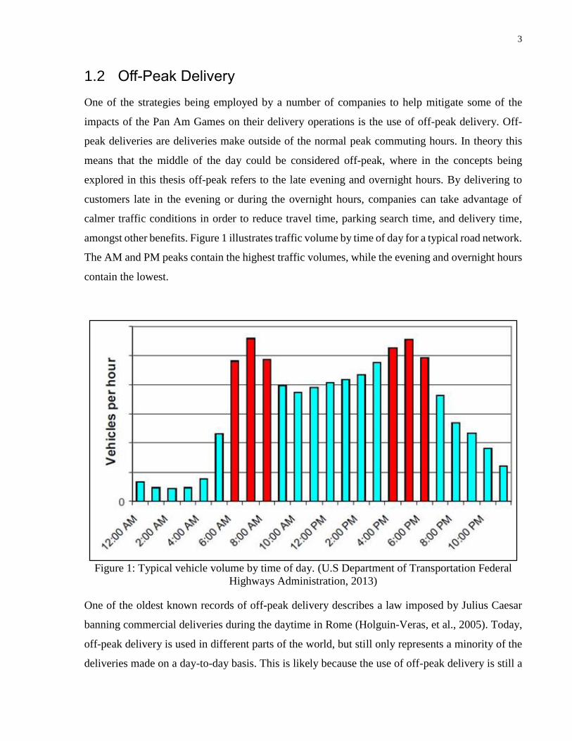
amongst other benefits. Figure 1 illustrates traffic volume by time of day for a typical road network.
The AM and PM peaks contain the highest traffic volumes, while the evening and overnight hours
contain the lowest.
Figure 1: Typical vehicle volume by time of day. (U.S Department of Transportation Federal
Highways Administration, 2013)
One of the oldest known records of off-peak delivery describes a law imposed by Julius Caesar
banning commercial deliveries during the daytime in Rome (Holguin-Veras, et al., 2005). Today,
off-peak delivery is used in different parts of the world, but still only represents a minority of the
deliveries made on a day-to-day basis. This is likely because the use of off-peak delivery is still a
4
highly debated issue. Large scale off-peak delivery programs can be successful, as was
demonstrated New York City’s restaurant sector (Holguin-Veras et al, 2007c), but there are certain
barriers that need to be overcome first. As part of their urban freight initiative, Metrolinx (2011)
listed off-peak delivery as one of their 17 actions they wish to improve upon in future work. In
their report they identified that the current barriers to off-peak delivery were restricted delivery
times due to noise bylaws, as well as the lack of incentive for companies and customers to
participate. For off-peak delivery to be accepted by both carriers and receivers, it is essential that
there be mutual benefits to both parties (Churchill, 1970).
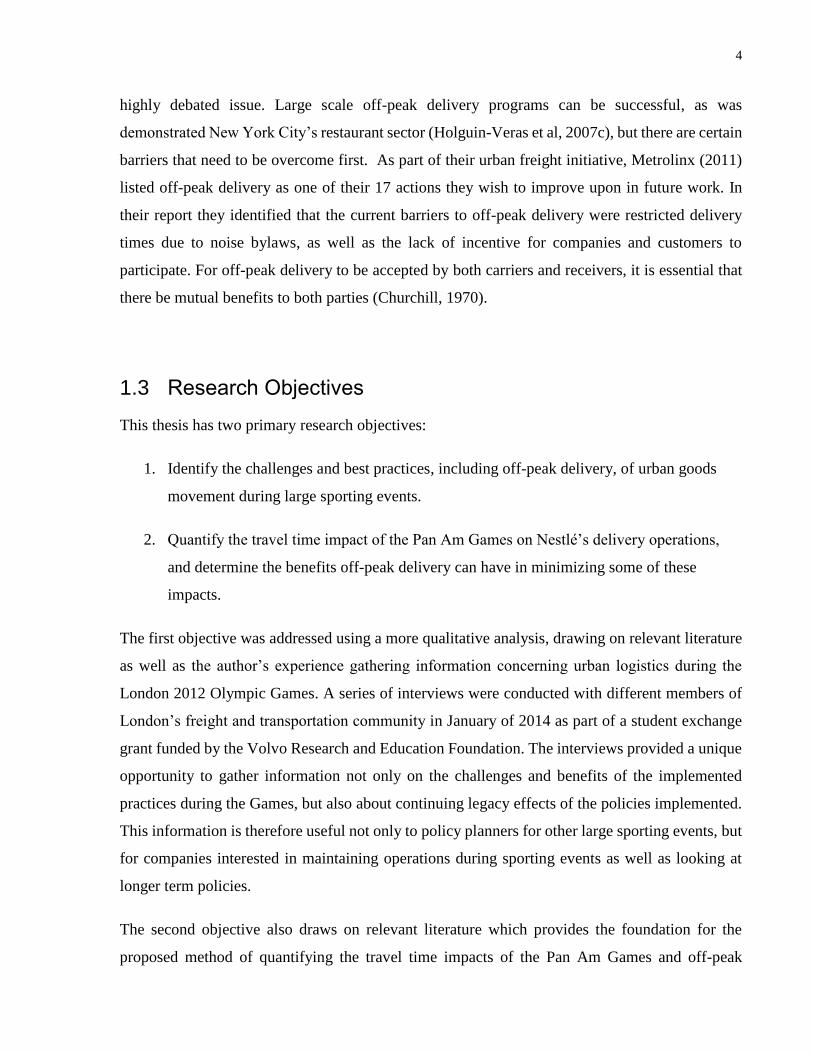
1.3 Research Objectives
This thesis has two primary research objectives:
1. Identify the challenges and best practices, including off-peak delivery, of urban goods
movement during large sporting events.
2. Quantify the travel time impact of the Pan Am Games on Nestlé’s delivery operations,
and determine the benefits off-peak delivery can have in minimizing some of these
impacts.
The first objective was addressed using a more qualitative analysis, drawing on relevant literature
as well as the author’s experience gathering information concerning urban logistics during the
London 2012 Olympic Games. A series of interviews were conducted with different members of
London’s freight and transportation community in January of 2014 as part of a student exchange
grant funded by the Volvo Research and Education Foundation. The interviews provided a unique
opportunity to gather information not only on the challenges and benefits of the implemented
practices during the Games, but also about continuing legacy effects of the policies implemented.
This information is therefore useful not only to policy planners for other large sporting events, but
for companies interested in maintaining operations during sporting events as well as looking at
longer term policies.
The second objective also draws on relevant literature which provides the foundation for the
proposed method of quantifying the travel time impacts of the Pan Am Games and off-peak

5
delivery. The specific goal was to determine the travel time impacts of the Pan Am Games on
normal delivery operations, and whether using off-peak delivery could yield any travel time
savings for carriers. A five step heuristic was created to estimate these travel time savings. This
heuristic identifies potential off-peak customers, determines if these off-peak customers should be
delivered to during the daytime or during off-peak hours, clusters the customers into routes using
a capacity constrained k-means clustering algorithm, and finally uses a simple vehicle routing
algorithm to determine the optimal routing and total travel time. Customer and delivery data
provided by Nestlé Canada and travel time data provided by IBI Group were used as inputs to the
heuristic to answer three questions concerning Nestlé delivery operations.
1. What will be the impact of the Pan Am Games on current Nestlé operations?
2. What are the benefits of planning routes one week at a time rather than on a call-and-
place basis for normal Nestlé operations outside of the Games?
3. Can off-peak delivery be used to mitigate the impacts from the Games?
4. Can advanced routing and off-peak delivery be used to reduce the total number of trucks
used?
The first question examines the impacts to Nestlé’s normal delivery operations should they make
no changes to their operations in preparation for the Games. This impact was estimated using travel
time estimates for the Pan Am Games travel conditions and compared against estimates as to what
the travel times would be without the Pan Am Games. The second question estimates the potential
benefits for advanced route planning against Nestlé’s current call-and-place delivery practices.
The third question focuses on the use of off-peak delivery in mitigating the impacts from the
Games. Different methods for off-peak customer selection were analyzed, and were meant to
represent different possibilities for customer participation in the off-peak delivery program. Finally
the possibility of reducing the number of total trucks used, and the impact on travel times was
examined. Further details concerning these three questions and their analysis can be found later in
the thesis.

6
1.4 Thesis Structure
This thesis is organized into eight chapters. The first chapter provides an introduction and outline
of the research goals and contributions. Chapter two introduces the London case study, and
outlines the findings of the qualitative analysis, including the list of best practices concerning
freight logistics during the London Olympic Games. Chapter three summarizes relevant literature
pertaining to goods movement and off-peak delivery, building on the findings of chapter two.
Chapter four introduces the Pan Am Games, outlines the expected conditions and challenges
specific to freight operation, and introduces the Nestlé case study. Chapter four also details the
data used for this project specific to the Nestlé case study. Chapter five reviews relevant literature
concerning different vehicle routing and clustering methods, and presents the heuristic
methodology used to analyze Nestlé’s operations during the Pan Am Games. Chapter six presents
the results of the analysis, and discusses the benefits of off-peak delivery and advanced planning
of Nestlé delivery operations. Finally, chapter seven provides a brief conclusion to the thesis
questions and touches upon the project limitations and possible future work.
7
Chapter 2
London Case Study
2.1 Purpose
In 2012, the summer Olympic Games were held in London, England. Over 10,000 athletes from
204 countries, as well as millions of spectators, descended on England for the 30th Olympic Games.
From a logistic perspective, these Games provided an excellent opportunity to examine the legacy
the Olympics had on freight stakeholders in London. Sponsored by the Volvo Research and
Education Foundation, and hosted by Michael Browne at the University of Westminster, the author
conducted a series of interviews with four organizations with different responsibilities for freight
logistics during the London Olympics. These four organizations were: TNT, Tradeteam, the
Freight Transport Association (FTA), and Transport for London (TFL). TNT is a global logistics
provider operating on a global scale delivery goods using a variety of transportation modes.
Tradeteam is a beverage carrier operating on a national scale in England. The FTA is an
organization of freight specialists who advise and work with freight operators around the country.
Finally, TFL is responsible for all of the public transit in London, as well as the operation of many
of the road networks in and around the city. These interviews were conducted to gain the following
information:
1. What was the company’s/organizations’ main role during the Olympics?
2. What logistic challenges were faced that were the direct result of the Olympics?
3. What strategies were used to deal with these challenges?
4. What went well? What didn’t go well? Would any changes be made in hindsight?
5. Are there any “legacy effects” that came as a result of policy changes implemented during
the Olympics?
As discussed above, the purpose of this case study is to identify a list of “best practices” concerning
freight delivery in London during and following the Olympic Games. The information gathered
supplements the quantitative analysis presented in later chapters of this thesis.
8
2.2 Freight and the Olympics
2.2.1 Challenges
As multi-sport sporting events, the Olympics and the Pan/Parapan American Games are
comparable in terms of the logistic challenges faced by their respective host cities. The experiences
gained during the London Olympics are particularly useful to the Toronto case study as many
similarities exist between the two events and cities. The Summer Olympics and Pan Am Games
(as well as Paralympics and Parapan Am Games) are roughly two weeks in duration, and contain
more than 7,000 athletes in each case. The Summer Olympics are the larger of the two with over
10,000 athletes participating. In terms of population, the GTHA and the Greater London Area are
home to 6 and 8 million people respectively. Both cities are the economic hub of their respective
regions and experience substantial traffic and freight movements on a daily basis. For the London
case, this made the efficient movement of athletes, officials and media, in addition to goods and
services a difficult task as the normal day-to-day activities could not be shut down for the duration
of the Olympics. A careful balance had to be struck between prioritizing the movement of athletes
and officials with the normal day-to-day commuters.
Part of the reason for hosting an event like the Olympics or the Pan Am Games is to showcase the
hosting cities to the world in order to promote tourism. Negative press resulting from chaotic traffic
conditions would hurt the image presented by the host cities. Employing proper traffic
management tools was essential to facilitate the movement of athletes, officials and media, who
make up the Olympic family, throughout the city during the Olympics. The principle method used
for this purpose was to create an interconnecting road network which restricted normal traffic and
allowed preferential access to the Olympic family. This interconnecting road network is known
either as the Games Route Network (GRN) or the Olympic Route Network (ORN), and the specific
segments of the road network are referred to as Games lanes.
The use of designated Games lanes has been a requirement of hosting the Olympics since after
the 1996 Atlanta Olympics (O'Sullivan, 2012) and a requirement for hosting the Pan Am Games
since 2011. The reasoning behind their use is to facilitate the movement of the Games family.
The 1996 Atlanta Olympics are notorious for the issues caused by transportation problems, with
several reports of athletes almost missing their events. The legacy was that by the 2000 Sydney
Games a Games Route Network was required for the bid by each host country. However, the
9
Olympic lanes were designed for moving athletes and other spectators to and from events, and
were not specifically designed for moving freight. In particular, turning and parking restrictions
along the ORN made delivering to customers in that region difficult. Specifics about the London
ORN is presented in the following section.
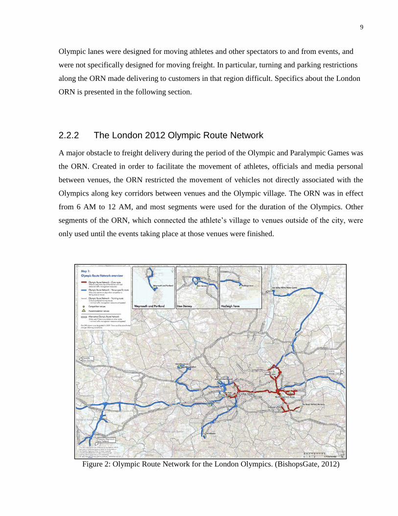
2.2.2 The London 2012 Olympic Route Network
A major obstacle to freight delivery during the period of the Olympic and Paralympic Games was
the ORN. Created in order to facilitate the movement of athletes, officials and media personal
between venues, the ORN restricted the movement of vehicles not directly associated with the
Olympics along key corridors between venues and the Olympic village. The ORN was in effect
from 6 AM to 12 AM, and most segments were used for the duration of the Olympics. Other
segments of the ORN, which connected the athlete’s village to venues outside of the city, were
only used until the events taking place at those venues were finished.
Figure 2: Olympic Route Network for the London Olympics. (BishopsGate, 2012)
10
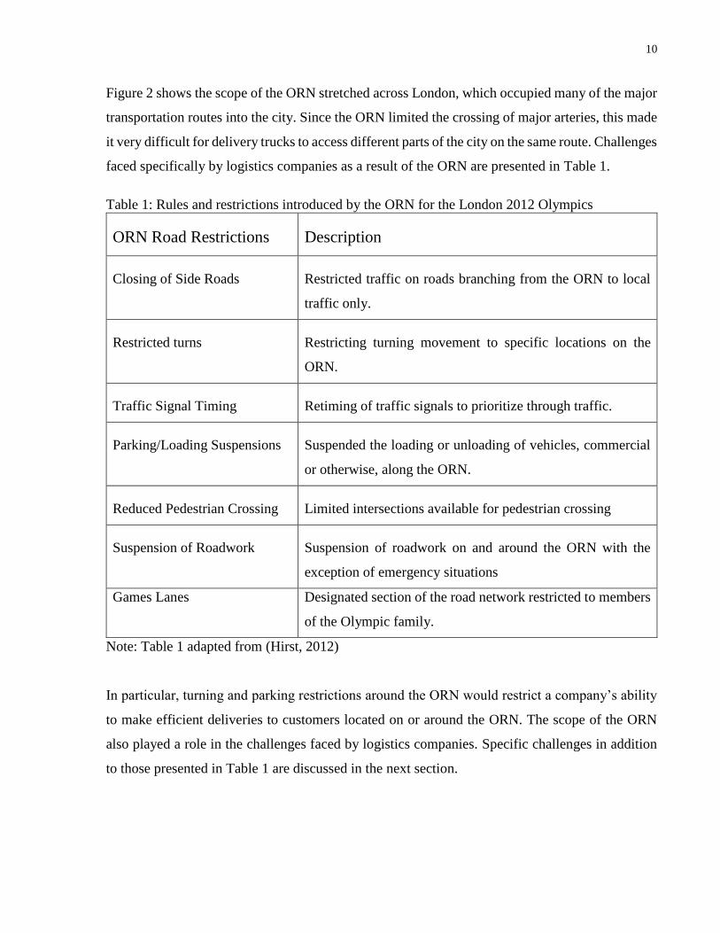
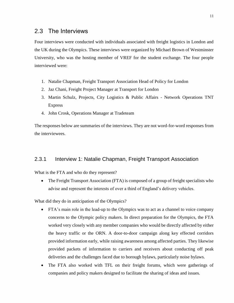
Figure 2 shows the scope of the ORN stretched across London, which occupied many of the major
transportation routes into the city. Since the ORN limited the crossing of major arteries, this made
it very difficult for delivery trucks to access different parts of the city on the same route. Challenges
faced specifically by logistics companies as a result of the ORN are presented in Table 1.
Table 1: Rules and restrictions introduced by the ORN for the London 2012 Olympics
ORN Road Restrictions Description
Closing of Side Roads Restricted traffic on roads branching from the ORN to local
traffic only.
Restricted turns Restricting turning movement to specific locations on the
ORN.
Traffic Signal Timing Retiming of traffic signals to prioritize through traffic.
Parking/Loading Suspensions Suspended the loading or unloading of vehicles, commercial
or otherwise, along the ORN.
Reduced Pedestrian Crossing Limited intersections available for pedestrian crossing
Suspension of Roadwork Suspension of roadwork on and around the ORN with the
exception of emergency situations
Games Lanes Designated section of the road network restricted to members
of the Olympic family.
Note: Table 1 adapted from (Hirst, 2012)
In particular, turning and parking restrictions around the ORN would restrict a company’s ability
to make efficient deliveries to customers located on or around the ORN. The scope of the ORN
also played a role in the challenges faced by logistics companies. Specific challenges in addition
to those presented in Table 1 are discussed in the next section.
11
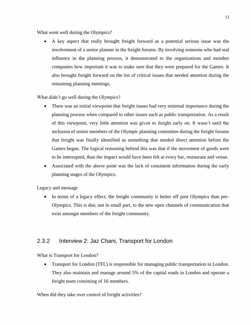
2.3 The Interviews
Four interviews were conducted with individuals associated with freight logistics in London and
the UK during the Olympics. These interviews were organized by Michael Brown of Westminster
University, who was the hosting member of VREF for the student exchange. The four people
interviewed were:
1. Natalie Chapman, Freight Transport Association Head of Policy for London
2. Jaz Chani, Freight Project Manager at Transport for London
3. Martin Schulz, Projects, City Logistics & Public Affairs - Network Operations TNT
Express
4. John Crosk, Operations Manager at Tradeteam
The responses below are summaries of the interviews. They are not word-for-word responses from
the interviewees.
2.3.1 Interview 1: Natalie Chapman, Freight Transport Association
What is the FTA and who do they represent?
The Freight Transport Association (FTA) is composed of a group of freight specialists who
advise and represent the interests of over a third of England’s delivery vehicles.
What did they do in anticipation of the Olympics?
FTA’s main role in the lead-up to the Olympics was to act as a channel to voice company
concerns to the Olympic policy makers. In direct preparation for the Olympics, the FTA
worked very closely with any member companies who would be directly affected by either
the heavy traffic or the ORN. A door-to-door campaign along key effected corridors
provided information early, while raising awareness among affected parties. They likewise
provided packets of information to carriers and receivers about conducting off peak
deliveries and the challenges faced due to borough bylaws, particularly noise bylaws.
The FTA also worked with TFL on their freight forums, which were gatherings of
companies and policy makers designed to facilitate the sharing of ideas and issues.
12
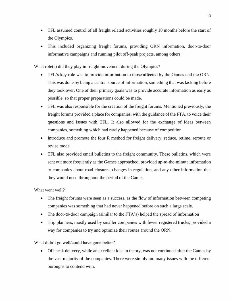
What went well during the Olympics?
A key aspect that really brought freight forward as a potential serious issue was the
involvement of a senior planner in the freight forums. By involving someone who had real
influence in the planning process, it demonstrated to the organizations and member
companies how important it was to make sure that they were prepared for the Games. It
also brought freight forward on the list of critical issues that needed attention during the
remaining planning meetings.
What didn’t go well during the Olympics?
There was an initial viewpoint that freight issues had very minimal importance during the
planning process when compared to other issues such as public transportation. As a result
of this viewpoint, very little attention was given to freight early on. It wasn’t until the
inclusion of senior members of the Olympic planning committee during the freight forums
that freight was finally identified as something that needed direct attention before the
Games began. The logical reasoning behind this was that if the movement of goods were
to be interrupted, than the impact would have been felt at every bar, restaurant and venue.
Associated with the above point was the lack of consistent information during the early
planning stages of the Olympics.
Legacy and message
In terms of a legacy effect, the freight community is better off post Olympics than pre-
Olympics. This is due, not in small part, to the new open channels of communication that
exist amongst members of the freight community.
2.3.2 Interview 2: Jaz Chani, Transport for London
What is Transport for London?
Transport for London (TFL) is responsible for managing public transportation in London.
They also maintain and manage around 5% of the capital roads in London and operate a
freight team consisting of 16 members.
When did they take over control of freight activities?
13
TFL assumed control of all freight related activities roughly 18 months before the start of
the Olympics.
This included organizing freight forums, providing ORN information, door-to-door
informative campaigns and running pilot off-peak projects, among others.
What role(s) did they play in freight movement during the Olympics?
TFL’s key role was to provide information to those affected by the Games and the ORN.
This was done by being a central source of information, something that was lacking before
they took over. One of their primary goals was to provide accurate information as early as
possible, so that proper preparations could be made.
TFL was also responsible for the creation of the freight forums. Mentioned previously, the
freight forums provided a place for companies, with the guidance of the FTA, to voice their
questions and issues with TFL. It also allowed for the exchange of ideas between
companies, something which had rarely happened because of competition.
Introduce and promote the four R method for freight delivery; reduce, retime, reroute or
revise mode
TFL also provided email bulletins to the freight community. These bulletins, which were
sent out more frequently as the Games approached, provided up-to-the-minute information
to companies about road closures, changes in regulation, and any other information that
they would need throughout the period of the Games.
What went well?
The freight forums were seen as a success, as the flow of information between competing
companies was something that had never happened before on such a large scale.
The door-to-door campaign (similar to the FTA’s) helped the spread of information
Trip planners, mostly used by smaller companies with fewer registered trucks, provided a
way for companies to try and optimize their routes around the ORN.
What didn’t go well/could have gone better?
Off-peak delivery, while an excellent idea in theory, was not continued after the Games by
the vast majority of the companies. There were simply too many issues with the different
boroughs to contend with.
14
Legacy and messages
The main legacy effect was the creation of the freight forums, which are still a twice yearly
occurrence.
2.3.3 Interview 3: Martin Schulz, TNT
What is TNT?
TNT is one of the world’s largest freight logistics companies, operating air, rail and truck
fleets.
TNT owns the largest market share of freight in the United Kingdom.
What were their preparations for the Olympics?
As with the other organizations, communications with their stakeholders was essential in
the success of TNT operations during the Games, such as keeping them informed of
changes in delivery patterns resulting from the ORN.
Normal operations consisted of deliveries made during the normal peak hours. A slight
shift to earlier departures was made for a portion of the Olympics. Delivery volumes were
increased and extra trucks were put onto the road to help deal with the potentially higher
delivery times. However, it was determined that this shift in start time and extra truck traffic
was not necessary, as the traffic conditions on the road were not as bad as anticipated.
Information packets were distributed to all truck drivers. These packets were route specific
and contained information about closures or restrictions on each individual route.
TNT had a different reaction to the outcomes than the other companies, as they found that their
normal operations were not significantly impacted. There was no legacy effect that was introduced
as a result of the Olympic planning.
15
2.3.4 Interview 4: John Crosk, Tradeteam
What is Tradeteam?
Tradeteam is a logistics company specializing in beverage delivery to bars and business.
What were their preparations for the Olympics?
Tradeteam started their Olympic planning two years before the start of the Games. The
planning involved an open doors policy which allowed their customers to see what
Tradeteam was doing to prepare, and hopefully get some ideas as how best to prepare
themselves.
Tradeteam also worked closely with the different boroughs, specifically about off-peak
delivery regulations. In many of the boroughs off-peak delivery wasn’t allowed due to
noise restrictions. Steps were made to create a “common sense” approach to night delivery
that would allow for fewer complaints during the Games.
Consolidating alcohol deliveries with other (food etc.) deliveries so that fewer trucks would
have to be on the road.
Off-peak deliveries were conducted along some corridors affected by the daytime ORN.
What didn’t go well/could have gone better
Planning team neglected to prepare for deliveries that were made to cities other than
London. Some Olympic events were held outside of the city and across the country. Some
distance deliveries to some of these locations were affected by the Games but not properly
prepared for.
Legacy and messages
Start planning for the Games early, and involve your customers in the discussion from the
beginning.

16
2.4 Common Themes and Best Practices from London
This section will outline some of the key lessons learned from personnel involved in logistics
planning for the London Olympic Games. These “best practices” are not specific to the Olympic
Games in London, but can be applied for any major sporting events, including the Pan Am Games.
2.4.1 Lesson 1. Plan for freight movement well in advance
Proper transportation planning takes a good deal of time. There will always be new issues that
arise and must be dealt with in order for the plan to be a success. In situations such as the Olympics
or Pan Am Games, the transportation discussion is usually centered on the movement of people
rather than the movement of freight. Stressing to the Games planners about the importance of
freight delivery to the success of the eventual success of the Games is essential. This involves
proactive organization on the part of local freight authorities, as well as a freight presence during
the planning process.
2.4.2 Lesson 2. Involve senior planners in the freight discussion
According to Natalie Chapman and Jaz Chani, of the FTA and TFL respectively, freight was not
being recognized as an issue of concern until after a senior Olympic planning official was involved
in the planning process. Bringing a senior official to the freight forums accomplished two things.
Firstly it sent the message to the contributing companies that freight movement during the
Olympics was a serious issue, and that without proper planning the companies would struggle with
their deliveries for the duration of the Games. Secondly it demonstrated to the senior official the
potential consequences if they were to do nothing. The senior planner’s involvement allowed for
the concerns of the freight community to be heard directly by the planning department. This was
considered to be an essential step for logistics planning.
17
2.4.3 Lesson 3. Freight forums are an essential part of planning efforts
The consensus amongst all of the interviewees was that the freight forums were the most useful
tool in preparation for the Olympic Games. Freight forums were an organized effort for affected
transportation and delivery companies, as well as those receiving freight, to be involved in an
ongoing discussion to assist with their planning. This was is not only an excellent method for
spreading information, but the open discussion concept brought forward ideas and issues that were
previously unknown. The forums brought together competing companies and planning officials,
and set the groundwork for many of the successful initiatives. These freight forums are still held
on a semi-annual basis, and are one of the legacy effects of the freight planning that went into the
Olympics.
2.4.4 Lesson 4. One consistent, reliable source of information to the stakeholders
It is essential that all of the stakeholders are receiving information from the same source. Before
TFL took over the freight management 18 months prior to the Olympics, information provided to
the stakeholders was not distributed consistently, and was not optimal. Aside from the introduction
of the freight forums, TFL also provided a consistent stream of information to the freight
community. This included weekly bulletins leading up to the Games, daily or twice daily bulletins
during the Games, ORN information, route planning assistance and any other support needed. This
allowed 91% of businesses surveyed to feel like they were prepared for the Games (Browne et al.
2014).
2.5 Summary and Olympic Freight Legacy
Members of the freight community in England faced many challenges during the Olympics which
impacted their ability to make deliveries. The main challenge was the implementation of the ORN,
which reduced access to certain key sections of the road network. Careful planning and
coordination between members of the freight community allowed for success both in terms of
Games time operations as well as legacy impacts. The overarching theme consistent across all four
of the lessons presented is the idea of communication. From the perspective of the overall city

18
planning it is essential to involve freight from the beginning. Having a voice in the early stages
allows for the concerns of the freight community to be heard. From the perspective of individual
companies it is essential to have an open line of communication with their customers. Starting the
conversation with customers far in advance of the event will help insure successful Game time
operations. It allows companies time to plan out their operations and procedures for the events,
while informing customers of potential changes to operations and allowing them to have a say into
their specific preferences. Finally, during the events it is important to have updated information
concerning the road network and the Games lanes in order to help companies deal with last minute
changes or incidents.
The transportation aspects of the 2012 Olympics were deemed a success by many of the parties
involved. The regular traffic experienced a shift in time period, with off-peak hours experiencing
a 13% increase in central London, while peak hours experienced a decrease by up to 12% (Browne
et al. 2014). As a result of Transport for London and the FTA’s pre-Game initiatives, 91% of
businesses and 81% of freight operators were prepared for the Olympics (Browne et al., 2014).
Both Browne et al. (2014) and Transport for London (2013b) indicate that over 50% of carriers
and receivers made changes to their normal operations in response to TFL and the FTA’s
initiatives. Of the four R’s outlined above, reduce was the most popular, with almost 50% of
stakeholders participating. This was followed by re-time with 41% and 45% for carriers and
receivers respectively, and reroute with 42% of carriers and only 5% of receivers (TFL. 2013b)
(Browne et al. 2014). The revise route strategy had very little participation, probably due the lack
of alternative options for most deliveries. TFL provided route planners online to aid businesses
with rerouting their trucks, while the FTA worked closely with carriers and receivers on off-peak
delivery (TFL. 2013b).
The lasting impacts and legacy of the freight management during the Olympic Games were less
successful than anticipated. Only 7% of carriers continued with the operational measures used
during the Olympics. Two reasons for this was a related lack of support from receivers, and noise
bylaws, which in the case of off-peak delivery had been eased during the Olympics to facilitate
off-peak delivery (Browne et al. 2014) (TFA. 2012). Positive legacies of the Olympic Game efforts
included the freight forums, spearheaded by the FTA, as well as the off-peak delivery projects.
However, there needs to be considerable collaboration with local municipalities before off-peak
delivery becomes commonplace as a routine consideration (FTA. 2012).

19
Chapter 3
Literature Review: Off-Peak Delivery
Off-peak delivery is the delivery of goods during the evening and overnight hours. A successful
off-peak delivery program requires cooperation and communication between receivers and
carriers, as well as a careful balance between the benefits and challenges associated with delivering
during off-peak hours. This literature review will outline in detail the benefits and challenges of
off-peak delivery, and will introduce the different methods carriers can use for off-peak delivery
and will conclude with a summary of key points.
3.1 Benefits and Challenges of Off-Peak Delivery
There has been extensive work conducted on the benefits and challenges of off-peak delivery in
New York City’s restaurant and business sector. Professor Jose Holguin-Veras and his research
group at the Rensselaer Polytechnic Institute have been responsible for a large portion of the
current research examining the impacts and challenges of off-peak delivery. The scope of their
research includes studies on the economic impact of off-peak delivery, studies on the variation of
travel times and speeds, pilot projects involving New York City’s restaurant sector, and a particular
focus on carrier receiver relationships.
The possible benefits of off-peak delivery can be broken down into benefits incurred while
travelling to and from customers, and benefits incurred during the drop-off or pick-up. The lowest
traffic levels are generally experienced during the overnight hours. Logically, this should
correspond to a range of benefits; including but not limited to: shorter travel time, higher travel
speeds, less idle time, and fewer emissions. However, the benefits experienced are likely to be
different for each carrier/receiver pair. Carriers whose tours contain only a small number of
customers located outside the central business district may experience different benefits and
challenges compared to those who usually make many stops in the downtown core on a regular
basis. Similarly, the type of customers being delivered to will have an impact.

20
Holguin-Veras et al. (2014b) organized a pilot off-peak delivery project which moved the delivery
schedules of 33 food delivery companies to off-peak hours. The trucks were monitored using GPS
technology to determine location and speed on an ongoing basis. Results from this project align
with what was expected in terms of the potential benefits of off-peak delivery. A speed increase
between the depot and first customer was observed, from 11.8 mph to 20.2 mph, while a smaller
increase was found while traveling between subsequent customers. These changes lead to a large
economic benefit which, when extrapolated for all freight across the entire city, were estimated at
roughly $147 million to $193 million in potential savings per year. In addition to these travel time
improvements, it was estimated that the delivery time during the pilot project was on average a
half of what would normally be experienced during the morning hours, when the majority of the
deliveries would have taken place.
There are further benefits that can be expected in addition to travel time improvements. Making
deliveries in urban areas can be difficult due to the lack of proper truck parking. It is estimated that
upwards of 96,000 additional vehicle kilometers are travelled every year on an average city block
due to the search for parking (Shoup, 2005). For commercial vehicles, the additional parking
search time is likely to have a significant impact on their total tour time. In addition, the delivery
of many types of goods requires parking nearby to the delivery location, either due to size or weight
of the products. As a direct result of this, many commercial vehicles are forced to park illegally
closer to their delivery location, resulting in parking tickets. For example, in 2012 Toronto
commercial vehicles accumulated $27 million in parking fines (Wenneman, Habib, & Roorda,
2014). In Toronto this issue is further impacted by the recent crackdown on illegal parking during
the morning peak hours by the City of Toronto (Moore, 2015). Fines of up to $1000 per month per
truck are not uncommon in New York for some companies (Holguin-Veras et al. 2014b). Holguin-
Veras et al. (2007c) indicates companies paying more for parking fines would be more likely to
switch to off-peak delivery in an attempt to reduce operating costs.
Several studies have shown the potential of off-peak delivery in reducing truck emissions. Yannis,
Golias, & Constantinos (2007) used a traffic simulation model to estimate the impact of delivery
time restrictions on truck traffic in Athens, Greece. Results of their analysis showed improvements
in overall traffic emmissons by restricting truck movement during peak hours. While not
specifically analyzing the effects of off-peak delivery on emissions, the results show the potential
benefits of reducing truck movements during the normal working hours. Campbell (1995)
21
generated analytical models to estimate emissions from large trucks in the Los Angeles area.
Results of the study were more inconclusive in terms of the total emissions reduction. The results
indicated that emissions reductions were possible, but only under conditions where the average
speed increased. For the case of Los Angeles, where there were nightime restrictions on truck
movement in some areas, the increase in average speed is negated by the extra distance needed to
travel to avoid the restricted areas. The Barcelona nighttime delivery project showed the potential
for reducing the number of trucks required to make deliveries. The project showed that seven
smaller trucks which would normally make the daily deliveries could be replaced by two larger
trucks, which would normally not be able to manover through downtown peak hour traffic (Chiffi,
2014).
The implementation of an off-peak delivery program requires addressing a number of challenges.
The current limited use of off-peak delivery is an indication of the challenges that companies face
in implementing an off-peak delivery program. The three concerns that encompass most of the
issues faced are: noise restrictions when delivering near residential areas, receiver participation in
the off-peak delivery program, and the security issues associated with making deliveries at night.
Considerable research (Holguin-Veras et al. 2007a, 2007b, 2007c) suggests that the largest barrier
to off-peak delivery is receiver willingness or ability to accept off-peak delivery. The main reason
receivers do not accept off-peak delivery is the associated cost. If the business already operates
over off-peak hours then this isn’t an issue, but for many receivers who only operate during
daytime hours this presents a major barrier. The cost to receivers to staff their business outweigh
the potential benefits of off-peak delivery (Holguin-Veras et al. 2014b). Holguin-Veras et al.
(2007c, 2005) surveyed restaurants to determine their likelihood of accepting off-peak deliveries
given a financial incentive. The hypothetical incentives, or disincentives, offered were the
deduction of one worker’s salary from their taxes, an unspecified Government subsidy, an
unspecified tax cut, or an increase in shipping cost during peak hours. Survey findings indicated
that the first two options (deduction of one worker salary or Government subsidy) would be the
most effective in enticing receivers to switch to off-peak, with 50% of respondents responding
positively. The other two options both had lower than 50% positive responses, indicating they
would not be sufficient incentives to switch to off-peak delivery. The question left unanswered is
the value of the Government subsidies required for the off-peak program to be worthwhile.

22
A policy restriction to off-peak delivery exists in many municipalities. This surrounds noise
regulations and bylaws, which restrict what activities may be done at night. Nighttime noise is
likely to generate opposition to off-peak delivery projects from members of the community
(Holguin-Veras et al. 2014). Noise can come from a number of different sources during the
delivery. Moving products within the vehicle, both with or without a lifting device, loading and
unloading the ramp, backup beepers as well as closing doors all add to the noise produced during
the delivery (Holguin-Veras et al. 2014). Other possible sources are personnel-related and can
include the playing of music and unnecessary slamming of doors. Some types of noise can be
reduced or eliminated with driver training and self-discipline, but other types of noise require more
innovative solutions. Wang et al. (2014) and Holguin-Veras et al. (2014a) suggest some possible
solutions. Hybrid fuel or electric trucks produce less engine noise on average than diesel trucks.
Refrigeration units can be further isolated and insulated to reduce noise, and low noise lifts can be
purchased which operate at around 60 db. Alternatively ‘quiet’ truck beds or liners can be used
which minimize the noise caused by metal making contact with metal. In Barcelona delivery trucks
were refurbished to include many of the low noise technologies. This allowed for the success of
an off-peak delivery project which saw food being delivered to grocery stores around the city
during hours normally restricted by noise restrictions. Results of that study showed noise caused
by the delivery differed very little from ambient background noise (Chiffi, 2014).
In Toronto, noise bylaw 591 (City of Toronto, 2010) limits what type of activities may take place
during the overnight hours, in particular in residential zones. Toronto has many mixed use zones,
and as a result this noise bylaw is in effect for a large portion of the city overnight. A pilot off-
peak delivery project organized by Ontario’s Ministry of Transportation (2014) monitored the
noise levels of deliveries in downtown Toronto. The conclusions of the pilot project were that
“background hum” of the urban environment was able to mask the sounds of the off-peak delivery,
and that the noise produced in the residential areas was sufficiently low as to not bother the
residents. This last conclusion was reinforced by the fact that no complaints were received during
the pilot project from residents.
With nighttime delivery there is an inherent risk involved that is less present during daytime
delivery. The risk can be broken down into risk of driver injury due to the dark conditions, and
risk to the driver due to other persons (Brom, Holguin-Veras, & Hodge, 2014). Dark conditions
make curbside deliveries more dangerous due to the risk from other drivers, as oncoming traffic
23
may not be expecting deliveries to be taking place at that time of night. This can be overcome
through the use of proper reflective safety gear for the driver, or through the use of pylon barriers
to warn other drivers of hazards. The risks to drivers due to other people are likely harder to predict
and control. Precautions can be made, especially for the delivery of more valuable goods such as
the delivery of alcohol, but it is likely impossible to completely eliminate the risks. A survey of
carriers in the New York off-peak pilot project indicates that some drivers actually felt more secure
delivering during off-peak hours. Their major concern was the dangers from other drivers, which
are much more prevalent during the daytime. The quieter conditions at night allowed them more
freedom while making deliveries (Brom, Holguin-Veras, & Hodge, 2014).
3.2 Off-Peak Delivery Methods
Assisted delivery is the most common delivery method for daytime deliveries. It involves having
a person present in the store to accept deliveries. While obviously not an issue for daytime
deliveries, staffing the store during the off-peak hours can be expensive. Receivers that normally
staff their stores during the off-peak hours also wouldn’t have this issue, but customers that are not
normally open overnight would.
Not all deliveries must be received by an employee of a business or other type of establishment.
Different methods for unassisted or unassisted delivery exist, but are dependent on the type of
product being delivered and the business setup. Delivery lockers or staging areas are examples of
methods that do not require direct access to the store or business (Holguin-Veras et al. 2013). Both
methods require a space separate from the interior of the business premises where the delivery can
be placed. The downside is that some products, like perishable goods, frozen items or high value
goods require extra infrastructure that can be expensive. The upside is that the stores/businesses
can operate on normal hours and do not need to staff the store overnight.
Other options for unassisted delivery involve giving the driver access to the store, either through
the use of a key or electronic code (Holguin-Veras et al. 2013). The benefits are similar to the
staging area, which allow the driver to make the delivery without staff being present; however,
these methods are less expensive as they do not require a large amount of additional space for
24
deliveries to take place. An obvious downside surrounds driver security; whenever a new driver is
assigned to a route, the security measures in place would have to be altered.
Lock boxes and separate delivery lockers can be used for non-perishable goods delivery. Lock
boxes and lockers are separated, locked area which can be accessed by delivery personnel. They
allow for the secure storage of goods without giving the driver access to the store proper. Virtual
cages use a series of small sensors to monitor a small area of floor space in the store proper
(Holguin-Veras, 2014d). Drivers are allowed access to this small area inside the store proper where
they can leave the goods. The sensors are able to detect if the driver leaves the virtual cage and
enters into restricted areas of the store. This method is beneficial in that it doesn’t require the
construction of any additional lockers or storage locations, but does require the installation of the
motion sensing equipment.
The final option is to give the delivery driver complete access to the store proper. This method
allows for complete delivery of the products, but does require a certain level of trust by the
receivers. Drivers can either be given a copy of the key to the store, the code to the electronic lock,
or some combination of those two in order to allow them to make the deliveries independently.
Alternatively, if a company is delivering to multiple locations of the same store, for example
different locations of the same clothing store, than a company representative can follow the driver
around, allowing access to each individual store. This would ensure that the delivery drivers cannot
access the stores at any other time while still allowing for, mostly, independent off-peak delivery
of the products.
25
3.3 Summary
Research shows that the principle barrier to the implementation of off-peak delivery programs is
receiver participation. Receivers generally dictate when deliveries should arrive at the store. For
them to accept a change in delivery schedules it is essential that they perceive some benefits to
themselves. For many receivers that operate only during the normal working hours, this benefit
may simply not exist. The cost of staffing the store overnight, or the extra security concerns would
simply outweigh any benefits of receiving their delivery before the stores open in the morning.
This leaves the carriers with several options: tailor the off-peak routes for customers who would
be willing to accept off-peak deliveries; offer incentives to customers who normally would not
accept off-peak deliveries to accept them; or in the special case of major sporting events, encourage
the use of off-peak deliveries by emphasizing the challenges that stores might face in receiving
their goods in a timely manner. This last method was used in London to encourage participation
in companies that may have otherwise not chosen to participate. Each of these options have
disadvantages associated with them. Tailoring the off-peak routes for customers who are willing
to accept off-peak deliveries doesn’t require the cost of incentives, but may result in largely spaced
out routes, possible resulting in increased travel times. Offering incentives to certain customers
may allow companies to create more efficient off-peak routes, but at the additional cost of
providing those incentives. Finally, encouraging the participation of customers during sporting
events may increase participation during the sporting events, but does not provide much
framework for maintaining off-peak delivery operations after the event is finished.

26
Chapter 4
Toronto 2015 Pan Am Games
4.1 Pan Am Games
The Pan American Games are one of the largest multi-sport sporting events in the world. The first
official Pan Am Games were held in Buenos Aires, Argentina in 1951, and were attended by
around 2500 athletes from 21 nations from North, Central, and South America (Wikipedia, 2015).
The most recent Pan Am Games were held in 2011 in Guadalajara, Mexico, and were also the first
Games to use a Games Route Network to facilitate the movement of the Games family to and from
their events. The Toronto Pan Am Games are set to be the largest ever Pan Am event in terms of
the number of competing athletes, with over 7,000 athletes representing 41 countries.
Initial preparations for the Toronto Pan Am Games began in in 2009, after the final voting to
determine the host country. Toronto beat out Lima, Peru and Bogotá, Colombia for the right to
host the Games. The preparations included, amongst others, the construction of new venues, the
installation of the Union-Pearson Express rail service, and the creation and modelling of various
transportation demand management tools. These tools were used to estimate various travel and
road conditions, and to test the impact of these conditions on the movement of people and goods
throughout the GTHA. One of the main challenges in planning transportation for an event of this
size is the magnitude of the Games in terms of the location of the venues. For example, the rowing
event takes place in Saint Catherine’s Ontario, over 120 km from the athlete’s village in downtown
Toronto. This creates issues as the transportation policies had to be extended a large distance
outside of the City of Toronto, which in turn impacts more people commuting into the city to work.
Figure 3 shows the location of the venues across the GTHA.

27
Figure 3: Venue locations in the GTHA. Source: (Ontario, Volume one - Strategic Framework
for Transportation, 2014b)
The City of Toronto contains the highest concentration of venues with the largest continual
expected number of spectators. The athlete’s village, the Pan Am Ceremonies venue, and Pan Am
Park at Exhibition Place are all located in downtown Toronto. In particular, Pan Am Park is
expected to experience high numbers of spectators on a daily basis for the duration of the Games.
4.1.1 Expected Travel Conditions
During the Pan Am and Parapan Am Games there will be an estimated 250,000 spectators coming
to the GTHA, along with the 10,000 athletes and officials (Toronto, 2014). This additional demand
will have to be absorbed by the current road and transit networks. Estimates for the number of
additional travelers to each of the event venues were developed based upon the expected ticket
sales at those venues (Ontario, Volume one - Strategic Framework for Transportation, 2014b).
This was done for each day of the Games, and the estimated additional demands were added to the

28
normal expected travel conditions to estimate the total demand on the road network. The venue
with the largest expected number of spectators is the Pan Am Park, located at Exhibition Place in
downtown Toronto. Figure 4 shows the expected number of total spectators per day at the Pan Am
Park. Peaking at around 45,000 spectators for the first two days of competition, and maintaining
high levels of expected spectators for the duration of the Pan Am Games. Pan Am Park had no
planned events for the Parapan Am Games.
Figure 4: Expected spectator numbers at the Pan Am Park in downtown Toronto
Source: (Ontario, Volume one - Strategic Framework for Transportation, 2014b)
Having the knowledge of expected traffic conditions during the Games for different key regions
of the city would help companies plan their delivers during those days. Focus was placed during
the planning process on certain days that were expected to place the most strain on the
transportation network. Two days, July 11 and July 15, which are day one and five in Figure 4,
were identified as the two days with the highest expected volumes of traffic. July 11 has the highest
expected spectator movements, but falls on a Saturday. July 15 has a number of events expecting
large numbers of spectators taking place across the GTHA and falls on a Wednesday, and therefore
is expected to be one of, if not the worst day, for traffic during the Games. For this day, an hour
by hour impact assessment was conducted to identify key venues and segments of the road network
29
which were likely to cause high traffic conditions. It was determined that the most impacted areas
were likely to be the major highways leading to the venues, partially due to the additional demand,
but mostly due to the Games Route Network being in effect during this time.
4.1.2 2015 Pan Am Games Route Network
The Ministry of Transportation Ontario (MTO) is responsible for organizing and maintaining the
transportation network during the 2015 Pan Am Games. A significant portion of their
responsibility will be governing the GRN. Similar to the ORN used in London, the GRN consists
of key, interconnect road segments that will serve to transport the Games family to and from their
events. One lane in each direction will be designated as Games Lanes for every section of the
GRN. These lanes will not be exclusively for Games family vehicles, but will also count as high
occupancy vehicle (HOV) lanes and will permit vehicles with 3+ occupants during the Pan Am
Games and 2+ occupants during the Parapan Am Games, as well as transit vehicles (MTO 2014a).
Other vehicles will be restricted to the non-designated lanes, the penalty for illegally using the
HOV lanes being a ticket. The MTO will operate the Games lanes for the duration of the Pan and
Parapan Am Games.
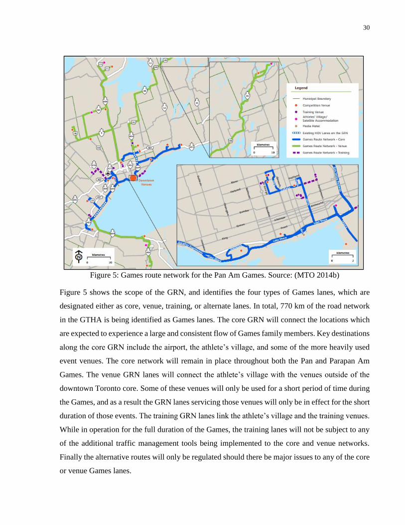
30
Figure 5: Games route network for the Pan Am Games. Source: (MTO 2014b)
Figure 5 shows the scope of the GRN, and identifies the four types of Games lanes, which are
designated either as core, venue, training, or alternate lanes. In total, 770 km of the road network
in the GTHA is being identified as Games lanes. The core GRN will connect the locations which
are expected to experience a large and consistent flow of Games family members. Key destinations
along the core GRN include the airport, the athlete’s village, and some of the more heavily used
event venues. The core network will remain in place throughout both the Pan and Parapan Am
Games. The venue GRN lanes will connect the athlete’s village with the venues outside of the
downtown Toronto core. Some of these venues will only be used for a short period of time during
the Games, and as a result the GRN lanes servicing those venues will only be in effect for the short
duration of those events. The training GRN lanes link the athlete’s village and the training venues.
While in operation for the full duration of the Games, the training lanes will not be subject to any
of the additional traffic management tools being implemented to the core and venue networks.
Finally the alternative routes will only be regulated should there be major issues to any of the core
or venue Games lanes.
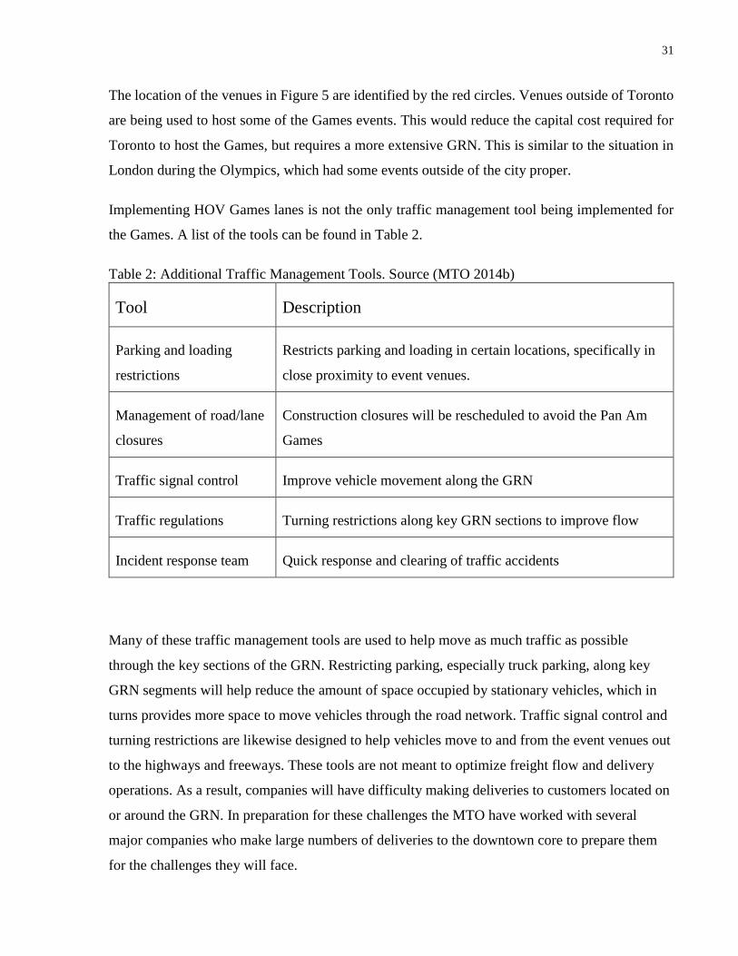
31
The location of the venues in Figure 5 are identified by the red circles. Venues outside of Toronto
are being used to host some of the Games events. This would reduce the capital cost required for
Toronto to host the Games, but requires a more extensive GRN. This is similar to the situation in
London during the Olympics, which had some events outside of the city proper.
Implementing HOV Games lanes is not the only traffic management tool being implemented for
the Games. A list of the tools can be found in Table 2.
Table 2: Additional Traffic Management Tools. Source (MTO 2014b)
Tool Description
Parking and loading
restrictions
Restricts parking and loading in certain locations, specifically in
close proximity to event venues.
Management of road/lane
closures
Construction closures will be rescheduled to avoid the Pan Am
Games
Traffic signal control Improve vehicle movement along the GRN
Traffic regulations Turning restrictions along key GRN sections to improve flow
Incident response team Quick response and clearing of traffic accidents
Many of these traffic management tools are used to help move as much traffic as possible
through the key sections of the GRN. Restricting parking, especially truck parking, along key
GRN segments will help reduce the amount of space occupied by stationary vehicles, which in
turns provides more space to move vehicles through the road network. Traffic signal control and
turning restrictions are likewise designed to help vehicles move to and from the event venues out
to the highways and freeways. These tools are not meant to optimize freight flow and delivery
operations. As a result, companies will have difficulty making deliveries to customers located on
or around the GRN. In preparation for these challenges the MTO have worked with several
major companies who make large numbers of deliveries to the downtown core to prepare them
for the challenges they will face.
32
4.1.3 Freight Planning Initiatives
In preparation for the Games, the MTO have been working with freight operators to ensure that
their operations can continue as normal and with as little impact from Games related activities as
possible. During the lead up to the Games, the MTO organized an informational campaign directed
at businesses concerning their transportation needs. This campaign was designed to inform
businesses of the challenges they would likely face during the Games, as well as provide some
potential solutions to those problems. The information to businesses was summarized in a
document titled ‘Keep Your Business Moving – Creating a Games Travel Plan’ (MTO 2014c).
The MTO outlines six steps for companies to follow to create a successful Games travel plan:
1. Understand Games operations and impacts
2. Access your workplace needs and activities
3. Make your commitment
4. Consider options and choose strategies
5. Detail your Games travel plan
6. Implement your Games travel plan
Steps two, three, five, and six require more effort on the part of the companies and less on the part
of the MTO. Step one, however, specifically requires the MTO to be able to provide accurate and
timely information to the different companies. Information concerning the GRN, event schedules,
and the expected congestion around the GTHA were released in February of 2014, more than one
year prior to the Games. This information will be supplemented with additional daily traffic
updates for the duration of the Games. This allows carriers not only to preplan for the Games, but
allows them to have the most up to the date information should any major incidents or changes
take place. The MTO has also made available a route planner which allows drivers, or companies,
to plan routes that avoid many of the Games lanes and venues (MTO, 2015).
As part of step four, consider options and choose strategies, the MTO encourages the use of the 4
R’s: reduce, retime, reroute, and revise mode which were used in London during the Olympics to
great effect. Reduce can mean two things. For office buildings and businesses where a large
number of people work, reduce means limiting the number of people that have to come into the
office on a daily basis. For example people could work from home and meetings could be held

33
remotely. For businesses who do attract many truck deliveries reducing means minimizing the
number of deliveries to the store through the use of consolidated deliveries. This is a
straightforward way for customers to receive the required number of products they need while
reducing the number of deliveries made during the Games. It would require a larger number of
trucks to be on the road in the period leading up to the Games, but a reduced number during the
Games when the conditions will be busier. The downside to this is that for customers in the food
industry, such as restaurants, grocery stores, and convenience stores, delivery larger quantities of
products further in advance is not possible due to storage issues or problems associated with
perishable goods.
Retiming deliveries requires shifting the hours of delivery. This can either be done by having the
trucks leave earlier or later from the depot, or by delivery products during the off-peak hours. This
would help avoid any of the issues associated with the expected congested conditions as well as
the GRN. As part of the retime option, the MTO was involved in organizing and testing the use of
off-peak delivery during the Games. The MTO pilot project conducted a customer satisfaction
survey post pilot project completion. Survey results showed for the most part a negative response
from receivers with respect to the off-peak delivery pilot project, as well as with the prospect of
receiving off-peak deliveries in the future. The main issues reported were a lack of communication
between managers and store employees, and issues with getting the stores stocked before the
morning rush should that customer fall late in the delivery schedule. A further pilot project was
planned for the spring of 2015 which hopes to improve upon these aspects. The positive outcomes
of the pilot project showed average speed increases and perceived ease of driving when compared
to daytime deliveries. One of the companies involved in the off-peak pilot was Nestlé Canada.
Nestlé delivers ice cream and other frozen products to a large number of customers in the GTHA.
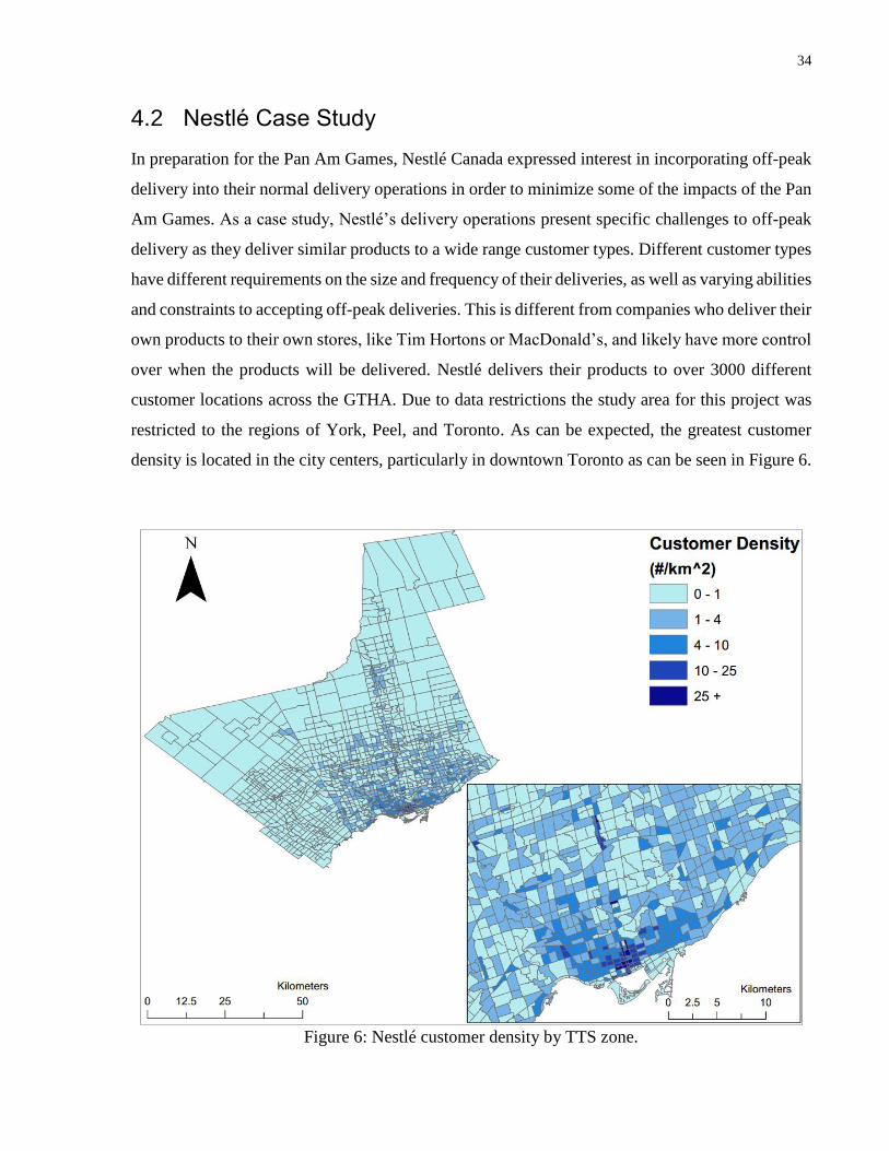
34
4.2 Nestlé Case Study
In preparation for the Pan Am Games, Nestlé Canada expressed interest in incorporating off-peak
delivery into their normal delivery operations in order to minimize some of the impacts of the Pan
Am Games. As a case study, Nestlé’s delivery operations present specific challenges to off-peak
delivery as they deliver similar products to a wide range customer types. Different customer types
have different requirements on the size and frequency of their deliveries, as well as varying abilities
and constraints to accepting off-peak deliveries. This is different from companies who deliver their
own products to their own stores, like Tim Hortons or MacDonald’s, and likely have more control
over when the products will be delivered. Nestlé delivers their products to over 3000 different
customer locations across the GTHA. Due to data restrictions the study area for this project was
restricted to the regions of York, Peel, and Toronto. As can be expected, the greatest customer
density is located in the city centers, particularly in downtown Toronto as can be seen in Figure 6.
Figure 6: Nestlé customer density by TTS zone.

35
The focus of this project was on Nestlé’s ice cream and frozen goods delivery in the GTHA. The
deliveries originate at Nestlé’s depot, which is located in Brampton Ontario. Nestlé currently
employs a call-and-place delivery model for their deliveries. In general, Nestlé’s customers request
deliveries at relatively consistent intervals. The most common requests are for one delivery per
week or one delivery every two weeks. Less frequently, customers will request two deliveries per
week, or one delivery per month. The frequency of deliveries to a specific customer are dependent
on the time of the year the deliveries are taking place; people are less likely to buy ice cream in
the winter; as well as the customer type and customer location. Larger customers, such as grocery
stores and department stores, are more likely to sell larger volumes of products as they experience
more traffic than convenience stores, and are therefore likely to require larger deliveries. Delivery
routes are generated every two days and only contain customers that have requested a delivery. A
benefit of this method is that it provides flexibility to Nestlé’s delivery operations, allowing them
make deliveries to customers on short notice. One of the downsides to this method is that it limits
the carrier’s ability to create efficient routes. Efficient routes in this case mean routes which have
customers relatively close to one another, limiting the total distance traveled.
4.3 Data
The data for the Nestlé case study was provided from three different sources. Travel time tables
were provided by IBI Group, a Toronto consulting firm responsible for developing Pan Am
Game’s traffic assignment models for the MTO. Information concerning Nestlé’s customers and
delivery operations were provided by Nestlé for this project. The information concerning the GRN,
particularly the location of the network and the venues, was obtained through documents publically
released by the MTO (MTO, 2014a; MTO, 2014b).
4.3.1 Travel Time Tables
Travel time tables were provided for the travel between Toronto, York and Peel regions, and travel
times were generated between all the different zones in each region. The zonal system used by IBI
Group is the 2011 GTHA Transportation Tomorrow Survey (TTS) zonal system, and the values
generated by the Emme model are zonal average travel times (DMG, 2011). The study region
contains a total of 1491 different TTS zones. The TTS zones are broken down between the regions
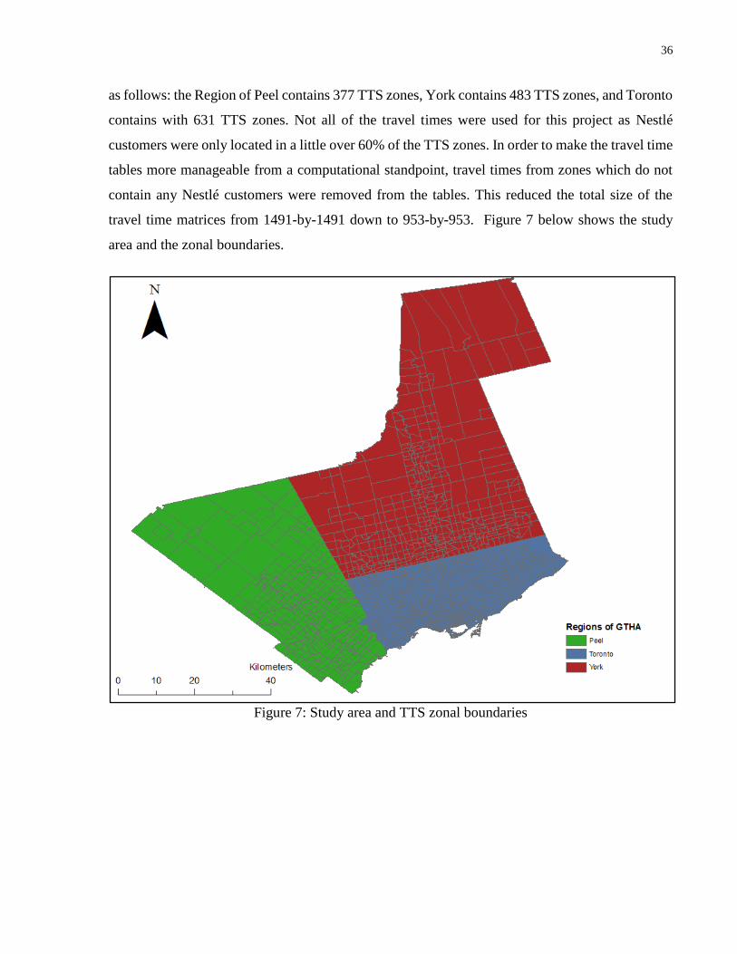
36
as follows: the Region of Peel contains 377 TTS zones, York contains 483 TTS zones, and Toronto
contains with 631 TTS zones. Not all of the travel times were used for this project as Nestlé
customers were only located in a little over 60% of the TTS zones. In order to make the travel time
tables more manageable from a computational standpoint, travel times from zones which do not
contain any Nestlé customers were removed from the tables. This reduced the total size of the
travel time matrices from 1491-by-1491 down to 953-by-953. Figure 7 below shows the study
area and the zonal boundaries.
Figure 7: Study area and TTS zonal boundaries
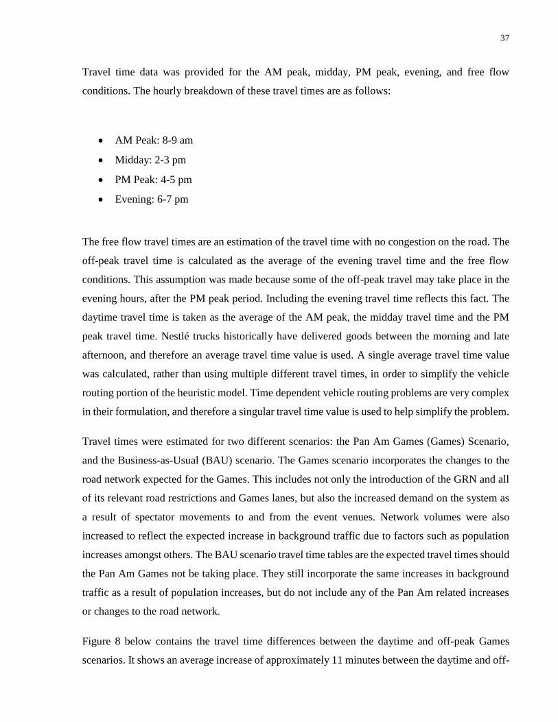
37
Travel time data was provided for the AM peak, midday, PM peak, evening, and free flow
conditions. The hourly breakdown of these travel times are as follows:
AM Peak: 8-9 am
Midday: 2-3 pm
PM Peak: 4-5 pm
Evening: 6-7 pm
The free flow travel times are an estimation of the travel time with no congestion on the road. The
off-peak travel time is calculated as the average of the evening travel time and the free flow
conditions. This assumption was made because some of the off-peak travel may take place in the
evening hours, after the PM peak period. Including the evening travel time reflects this fact. The
daytime travel time is taken as the average of the AM peak, the midday travel time and the PM
peak travel time. Nestlé trucks historically have delivered goods between the morning and late
afternoon, and therefore an average travel time value is used. A single average travel time value
was calculated, rather than using multiple different travel times, in order to simplify the vehicle
routing portion of the heuristic model. Time dependent vehicle routing problems are very complex
in their formulation, and therefore a singular travel time value is used to help simplify the problem.
Travel times were estimated for two different scenarios: the Pan Am Games (Games) Scenario,
and the Business-as-Usual (BAU) scenario. The Games scenario incorporates the changes to the
road network expected for the Games. This includes not only the introduction of the GRN and all
of its relevant road restrictions and Games lanes, but also the increased demand on the system as
a result of spectator movements to and from the event venues. Network volumes were also
increased to reflect the expected increase in background traffic due to factors such as population
increases amongst others. The BAU scenario travel time tables are the expected travel times should
the Pan Am Games not be taking place. They still incorporate the same increases in background
traffic as a result of population increases, but do not include any of the Pan Am related increases
or changes to the road network.
Figure 8 below contains the travel time differences between the daytime and off-peak Games
scenarios. It shows an average increase of approximately 11 minutes between the daytime and off-

38
peak travel times. This shows that while some significant travel time savings can be made during
the off-peak hours, half of the trips taken will experience between 0-11 minutes of travel time
savings. A similar analysis was performed which showed that the average percentage travel time
savings for all trips was around 37%.
Figure 8: TTS travel time difference between daytime and off-peak Games scenario.
The largest travel time savings in Figure 8 are for trips between zones located large distances apart.
The expected travel time differences for shorter trips between adjacent or nearby zones is much
smaller. Figure 9 shows the expected average travel time differences between adjacent zones by
switching to off-peak hours during the Pan Am Games. The average travel times for adjacent zonal
travel was determined for each zone for both the daytime and off-peak hours. The yellow sections
of the map show an average travel time decrease of under 30 seconds. Green sections contain
average travel time decreases of over 30 seconds, with the maximum being around 11 minutes.
Small travel time differences can be expected due to the small size of the TTS zones.
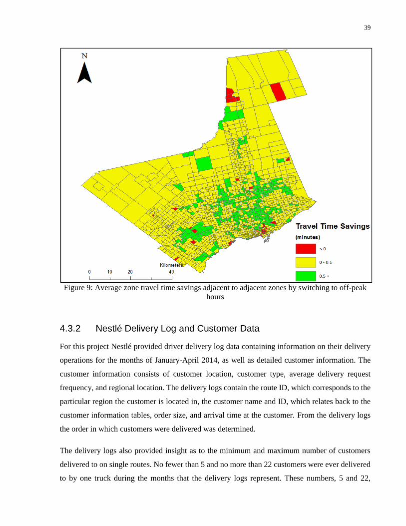
39
Figure 9: Average zone travel time savings adjacent to adjacent zones by switching to off-peak
hours
4.3.2 Nestlé Delivery Log and Customer Data
For this project Nestlé provided driver delivery log data containing information on their delivery
operations for the months of January-April 2014, as well as detailed customer information. The
customer information consists of customer location, customer type, average delivery request
frequency, and regional location. The delivery logs contain the route ID, which corresponds to the
particular region the customer is located in, the customer name and ID, which relates back to the
customer information tables, order size, and arrival time at the customer. From the delivery logs
the order in which customers were delivered was determined.
The delivery logs also provided insight as to the minimum and maximum number of customers
delivered to on single routes. No fewer than 5 and no more than 22 customers were ever delivered
to by one truck during the months that the delivery logs represent. These numbers, 5 and 22,

40
represent the lower and upper limits of Nestlé’s delivery operations and are considered hard limits
for route generation in the methodology. These limits are referred to as the minimum and
maximum route size constraint respectively.
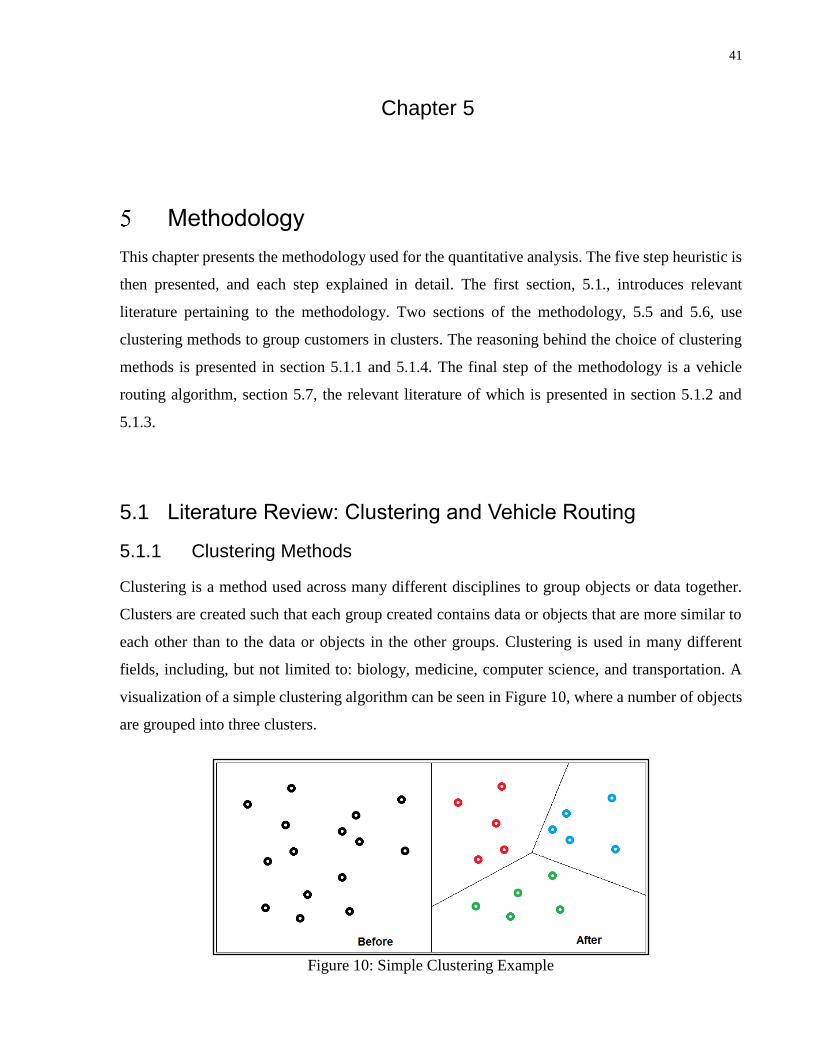
41
Chapter 5
Methodology
This chapter presents the methodology used for the quantitative analysis. The five step heuristic is
then presented, and each step explained in detail. The first section, 5.1., introduces relevant
literature pertaining to the methodology. Two sections of the methodology, 5.5 and 5.6, use
clustering methods to group customers in clusters. The reasoning behind the choice of clustering
methods is presented in section 5.1.1 and 5.1.4. The final step of the methodology is a vehicle
routing algorithm, section 5.7, the relevant literature of which is presented in section 5.1.2 and
5.1.3.
5.1 Literature Review: Clustering and Vehicle Routing
5.1.1 Clustering Methods
Clustering is a method used across many different disciplines to group objects or data together.
Clusters are created such that each group created contains data or objects that are more similar to
each other than to the data or objects in the other groups. Clustering is used in many different
fields, including, but not limited to: biology, medicine, computer science, and transportation. A
visualization of a simple clustering algorithm can be seen in Figure 10, where a number of objects
are grouped into three clusters.
Figure 10: Simple Clustering Example
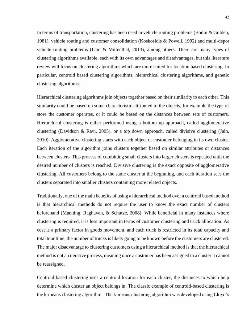
42
In terms of transportation, clustering has been used in vehicle routing problems (Bodin & Golden,
1981), vehicle routing and customer consolidation (Koskosidis & Powell, 1992) and multi-depot
vehicle routing problems (Lam & Mittenthal, 2013), among others. There are many types of
clustering algorithms available, each with its own advantages and disadvantages, but this literature
review will focus on clustering algorithms which are more suited for location based clustering. In
particular, centroid based clustering algorithms, hierarchical clustering algorithms, and genetic
clustering algorithms.
Hierarchical clustering algorithms join objects together based on their similarity to each other. This
similarity could be based on some characteristic attributed to the objects, for example the type of
store the customer operates, or it could be based on the distances between sets of customers.
Hierarchical clustering is either performed using a bottom up approach, called agglomerative
clustering (Davidson & Ravi, 2005), or a top down approach, called divisive clustering (Jain,
2010). Agglomerative clustering starts with each object or customer belonging in its own cluster.
Each iteration of the algorithm joins clusters together based on similar attributes or distances
between clusters. This process of combining small clusters into larger clusters is repeated until the
desired number of clusters is reached. Divisive clustering is the exact opposite of agglomerative
clustering. All customers belong to the same cluster at the beginning, and each iteration sees the
clusters separated into smaller clusters containing more related objects.
Traditionally, one of the main benefits of using a hierarchical method over a centroid based method
is that hierarchical methods do not require the user to know the exact number of clusters
beforehand (Manning, Raghavan, & Schutze, 2008). While beneficial in many instances where
clustering is required, it is less important in terms of customer clustering and truck allocation. As
cost is a primary factor in goods movement, and each truck is restricted in its total capacity and
total tour time, the number of trucks is likely going to be known before the customers are clustered.
The major disadvantage to clustering customers using a hierarchical method is that the hierarchical
method is not an iterative process, meaning once a customer has been assigned to a cluster it cannot
be reassigned.
Centroid-based clustering uses a centroid location for each cluster, the distances to which help
determine which cluster an object belongs in. The classic example of centroid-based clustering is
the k-means clustering algorithm. The k-means clustering algorithm was developed using Lloyd’s

43
algorithm as its foundation (Lloyd, 1982), although an improvement on the formulation, which is
now more commonly used, was developed in the 1970’s (Hartigan & Wong, 1979). The k in the
k-means stands for the number of clusters desired for the current data set. The algorithm works by
identifying initial starting centroid locations. While not actually centroids during the first iteration,
these locations will serve as starting points to which objects or customers will be assigned. Once
initial clusters are generated, the location of the centroid for that cluster can be recalculated. The
customers are then reassigned to centroids, and this process continues until the location of the
centroids does not change. Figure 11 shows an example of the clustering process.
Points to be clustered

44
After the first clustering iteration
15th clustering iteration

45
Final clustering results
Figure 11: Progression of k-means clustering algorithm
Figure 11 shows the progression of the k-means clustering algorithm. In this example 235
customers are clustered into 20 different clusters. The primary benefits of the k-means clustering
algorithm are the efficiency of the algorithm and the certainty about the number of clusters. The
number of trucks, and therefore the number of clusters, is likely going to be known before the
routes are generated. With the k-means algorithm the user sets this value, something that cannot
be done with hierarchical clustering. The k-means algorithm is also efficient in terms of run time
and relatively straightforward to add constraints to (Kim, 2007). A number of additions or
alterations to the traditional k-means method have been developed over the years.
One disadvantage of using a k-means clustering algorithm is that the results of the clustering are
dependent on the initial starting locations. Different starting locations for the cluster centroids may
result in different final clusters, even if everything else is kept constant. When clustering a small
number of objects it is possible to find the optimal solution by running the algorithm multiple times
for every combination of starting points, but this method quickly becomes too computationally
intensive for large numbers of objects or clusters. It is also possible for the k-means algorithm to
not converge on a final solution, which happens when certain object assignments and
reassignments results in a pattern of repeating object cluster configurations.

46
A genetic clustering technique was developed which utilizes a genetic algorithm to find optimal
clusters (Maulik & Bandyopadhyay, 2000). Genetic algorithms are used commonly for search and
optimization problems, and are based on the theories of evolution and natural selection (Mitchell,
1998). The initial conditions of the problem are initialized as what are referred to as chromosomes,
which are strings of numbers representing the current conditions of the problem. The fitness of
each set of chromosomes is calculated, similar to the initial solution of the problem. Sections of
the chromosomes are swapped or mutated with the purpose of trying to maximize the total fitness
of the problem. This process is repeated until the maximum fitness is calculated (Mitchell, 1998).
According to Maulik & Bandyopadhyay (2000), their genetic clustering algorithm is able to
outperform the standard k-means clustering algorithm for every scenario they tested. Genetic
algorithms are not restricted by one of the major shortcomings of the k-mean clustering methods,
they are more likely to determine the global minimum rather than run the risk of alternating
between local minima. The limitations of genetic clustering methods are their complexity,
difficulty of adaptation, and CPU time.
5.1.2 Vehicle Routing
The vehicle routing problem is one of the most thoroughly studied problems in transportation. In
the simplest form, the vehicle routing problem is equivalent to the travelling salesman problem
(TSP). The goal of the TSP is to minimize the total travel time or distance required to make a stop
at every location specified on the network while finishing at the starting location. However, real-
world examples are rarely as simplified as the TSP, and will often require additional constraints.
Common additions include the capacity constraint, time window constraints, and day of the week
constraints. Each variation of the vehicle routing problem adds additional complexity to its
formulation, increasing the computational requirements. Among the most common variation to the
TSP is the capacity constrained vehicle routing problem. This constraint can either limit the
number of deliveries each truck can make based on the trucks physical capacity, or the length of
the tour based on the number of stops, the total distance travelled, or the total time spent on the
road (Augerat et al, 1998). Capacity constraints are common in multiple vehicle TSP (m-TSP)
problems, as well as many more complex vehicle routing formulations.

47
A second common variation to the standard vehicle routing algorithm is the vehicle routing
problem with time windows (VRPTW). The reason for this variation is that some customers may
be unavailable during certain times of the day to accept deliveries, and this reality must be reflected
in the vehicle routing model. Travel times, starting times, and delivery times are used to estimate
the time in which a delivery would take place at a certain customer. The VRPTW problem can be
separated into two formulations: hard formulations and soft formulations (Kallehauge, Larsen ,
Madsen, & Solomon, 2005). Hard VRPTW have strict time windows in which the delivery is to
take place, and should a solution propose delivery to a customer outside of their requested time
window, that solution would be rejected. Soft time windows will allow for deliveries outside of
the specific time windows, but will impose a penalty to the system.
The periodic vehicle routing problem extends the regular vehicle routing problem to m days of
delivery. For example, instead of performing 50 deliveries using 5 trucks on one day, the company
would perform 10 deliveries a day using one truck. This method takes into account a customer’s
delivery availability, similar to the time windows constraint but over days instead of hours. The
periodic vehicle routing problem can also be formulated to deal with customers who require more
than one delivery in a short amount of time. These customers can therefore be included in routes
on separate days without having to redo the entire vehicle routing algorithm.
5.1.3 Subtour Elimination
In many cases, the optimal conditions resulting in the minimum total travel time and which satisfy
all the constraints of a vehicle routing algorithm will not be a complete tour. A complete tour is
one in which the vehicle in question will stop at all the customers on its route, and then return back
to the depot. It is possible, and likely in many cases, that the generated truck route will contain
subtours. A subtour is a group of at least two customers that are not connected to the depot via the
generated route. The problem is that the basic constraints of the vehicle routing problem do not
account for this issue, and therefore specific subtour constraints have to be formulated in order to
generate reasonable results.
The difficulty in eliminating subtours is not in the constraint generation, but in the number of
constraints that are required to eliminate all possible subtours. The total number of subtours

48
consists of all possible combinations of customers from the total list. For example, a group of
twenty customers contain over 500,000 possible subtours. The complete list of subtours is actually
over one million, but for each set of customer’s each subtour contains an associated subtour made
up of the remaining customers. The result is that by eliminating one particular subtour its pairing
subtour is also eliminated. For example, a constraint which prohibits a subtour containing
customers 1-5 in a 10 customer vehicle routing problem would also eliminate the subtour
containing customers 6-10. The sheer number of constraints needed for even small problems
makes it so that eliminating all subtours at once is impossible. As a results, several methods were
developed to eliminate subtours without having to add all constraints.
The cutting plane method of subtour elimination takes advantage of the fact that the vast majority
of possible subtours are not likely to appear in the potential solution for a vehicle routing problem.
The cutting plane method starts with no subtour constraints and allows the vehicle routing
algorithm to solve for the optimal solution. After the solution is found there is a check to identify
any subtours in the solution. For each subtour found, a constraint is formulated and added into the
vehicle routing algorithm, and the problem is resolved. This continues until no subtours are found
in the solution.
5.1.4 Cluster-First Route Second-Models
An alternative way to route multiple vehicles is by using a cluster-first method. A benefit of using
this method is that it can reduce a complicated vehicle routing problem to a series of less complex
formulations. Clustering can incorporate the capacity constraint algorithms as well as some of
those required for the periodic vehicle routing problem. They can do this by limiting the size of
the cluster, either in terms of truck capacity or the number of customers, or by clustering similar
customers together, for example customers that can only be serviced on one day of the week.
Cluster-first methods are unable, however, to eliminate the time window requirements for VRPTW
problems, as the time window constraints are essential to the delivery order of the customers.
Common examples of cluster-first route-second vehicle routing models include the Fisher and
Jaikumar heuristic, the Petal Algorithm, and the sweep algorithm.

49
The sweep algorithm is a very simple method of clustering. The concept is to generate clusters by
performing a rough ‘sweep’ of the customers, meaning generating an imaginary line from the depot
as the starting point, and moving a secondary line from the first in a rotational movement similar
to the hands of a clock. The rotation stops when the trucks capacity is met or the target number of
customers are contained in the cluster. After the clusters are created, a vehicle routing algorithm
can be performed for each cluster. Figure 12 shows a visualization of the sweep algorithm for a
simple three cluster example.
Figure 12: Example sweep algorithm method for customer clustering
The main benefit of the sweep algorithm is its simplicity. It can be performed quickly for large
numbers of customers if necessary. The downside is that because of its simplicity, it does not take
into account actual travel time or customer distances, and is usually only effective with a central
depot location. The sweep algorithm is typically outperformed in terms of overall travel time
results by more involved algorithms such as the petal algorithm and the Fisher and Jaikumar
50
heuristic. The improved petal algorithm (Renaud, Boctor, & Laporte, 1996) is similar to the sweep
algorithm with the exception that it allows for multiple routes within one ‘sweep’ of the customers.
The Fisher and Jaikumar heuristic solves a general assignment problem to generate the clusters
(Fisher & Jaikumar, 1981). Seed customers are identified as the starting point for the customer
assignment to specific trucks and the general assignment problem assigns other customers to these
trucks.
Geetha, Poonthalir, & Vanathi (2009) introduced a cluster-first route-second method which
incorportates a k-means clustering algorithm specifically designed for the capacitated vehicle
routing problem. The benefits of this method were the relative simplicity in which changes or
additional constraints could be added to the algorithm. The results showed this method was
competitive with other vehicle routing heuristics in terms of travel times and computational times.

51
5.2 Nestlé Case Study Methodology
There were four specific research objectives identified in section 1.3 of this thesis concerning the
Nestlé case study. The first objective analyzed the travel time impacts the Pan Am Games would
have on Nestlé’s normal operations. The method used for this objective was straightforward, and
involved comparing the Pan Am Games travel times versus the business-as-usual travel times
using the driver delivery logs to determine the customer deliver order. The methodology used for
objectives 2-4 used the heuristic presented in this chapter. The methods used are a five step process.
This chapter will outline this process and provide details into the assumptions and specific methods
used to evaluate off-peak delivery potential. The five steps of this process are introduced in Figure
13:
Figure 13: Five step heuristic methodology
Step 1: Identify Potential Off-Peak Customers
Step 2: Potential Off-Peak Customer List Refinement
Step 3: Off-Peak Customer Selection for Clustering
Step 4: Capacity Constrained K-Means Clustering
Step 5: Vehicle Routing

52
The first step of this process is identifying potential off-peak customers. These are customers that
have to potential to be serviced in the off-peak hours. Multiple methods of customer identification
were tested, with customers either identified by type or by proximity to the GRN. The second step
of this process refines the list of potential off-peak customers based on several factors. In this
context, refining the list of potential off-peak customers means identifying potential off-peak
customers that could be serviced during the off-peak hours, but that should be serviced during
daytime hours. The third step involves selecting off-peak customers from the list of potential off-
peak customers. The customers are selected either randomly or more strategically from the list of
potential off-peak customers. The number of customers selected for delivery during the off-peak
hours depends on the number of trucks being used during the off-peak hours and the capacity of
those trucks. The fourth step of the heuristic groups the off-peak customers selected in the third
step into different clusters. This same process is applied separately to the off-peak customers and
the remaining daytime customers. Each cluster generated represents the deliveries made by one
truck during either the daytime or off-peak hours, and the number of clusters depends on the
number of trucks identified in the third step. The fifth and final step is a simple vehicle routing
algorithm, which determines the optimal routing for each cluster generated using the k-means
clustering algorithm.
This five step process is a heuristic model for analyzing the potential impacts and benefits of using
off-peak delivery. The purpose of this analysis was fourfold: to estimate the impact of the Pan Am
Games on normal Nestlé operations, to estimate the benefits of using advanced routing techniques
on total travel times, to estimate the impact of using off-peak delivery during the Pan Am Games
to mitigate some of the expected operational challenges, and to determine if a reduction in the
number of vehicles used is possible. Some assumptions were made during the creation of this
heuristic. A single truck size, in terms of capacity, was assumed in order to simplify the clustering
and vehicle routing problem. The number of customers assigned to a single route were also limited
by the data available in the Nestlé delivery logs, presented in section 4.3.2, which showed the
maximum route size to be 22 customers, and the minimum route size to be 5 customers.

53
5.3 Identifying Potential Off-Peak Customers
This step of the heuristic is used to identify customers that have the potential to accept off-peak
deliveries. A total of two identification methods were used to identify potential off-peak
customers:
1. Identification of potential off-peak customers based on customer type.
2. Identification of potential off-peak customers based on customer proximity to the GRN.
Off-peak customer identification based on customer type identifies potential off-peak customers
based on what type business they operate. This type of customer identification is based on the
assumption that some customers are more likely to be able to accept off-peak deliveries than other
customers. This is either because they already operate during the off-peak hours, or have the ability
to accept unassisted off-peak deliveries. Identifying customers willing to accept off-peak deliveries
without incentives would help reduce the cost of Nestlé’s off-peak delivery program, should they
choose to use incentives as a tool to attract customers.
Off-peak customer identification based on distance to the GRN identifies customers in close
proximity to the GRN. These may not necessarily be customers who would normally accept off-
peak deliveries, however, due to their proximity to the GRN they may experience negative impacts
from the Games due to the GRN restrictions. This impact, or unreliability of service, is the potential
delay in deliveries due to the travel conditions around the GRN as well as the parking and stopping
restrictions for delivery trucks. The assumption is that these customers may be willing to accept
off-peak deliveries, at least for the duration of the Pan Am Games, as deliveries during off-peak
hours would not experience these impacts.
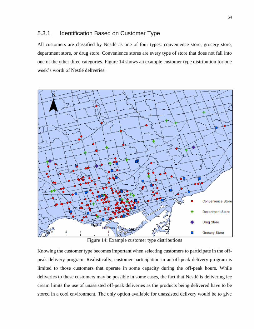
54
5.3.1 Identification Based on Customer Type
All customers are classified by Nestlé as one of four types: convenience store, grocery store,
department store, or drug store. Convenience stores are every type of store that does not fall into
one of the other three categories. Figure 14 shows an example customer type distribution for one
week’s worth of Nestlé deliveries.
Figure 14: Example customer type distributions
Knowing the customer type becomes important when selecting customers to participate in the off-
peak delivery program. Realistically, customer participation in an off-peak delivery program is
limited to those customers that operate in some capacity during the off-peak hours. While
deliveries to these customers may be possible in some cases, the fact that Nestlé is delivering ice
cream limits the use of unassisted off-peak deliveries as the products being delivered have to be
stored in a cool environment. The only option available for unassisted delivery would be to give

55
drivers access to the store freezers or cold storage facilities so the products being delivered do not
melt before the store opens in the morning.
The following assumptions were made to simplify the customer selection process.
1. Grocery stores, department stores, and drug stores stock shelves at night, and are
therefore able to accept off-peak deliveries.
a. The first assumption is based upon an internet search for job postings in the
GTHA. There were numerous job postings for night crew positions at major
grocery stores (Loblaw’s, Sobeys, No-Frills, Metro), as well as for department
stores (Walmart) and drug stores (Shoppers Drug Mart).
2. Convenience stores are not open during off-peak hours, and therefore are not able to
accept off-peak deliveries, with the following exceptions:
a. 7-Eleven stores, which are categorized as convenience stores, are all open 24-hrs
per day according to their website.
b. Gas stations, which are categorized as convenience stores, are open overnight and
are able to accept off-peak deliveries. This is based on an online survey of the
different gas stations in the GTHA reveals that the three major operators, Shell,
Esso and Petro-Canada, all operate the majority of their stores 24-hrs per day.
c. Mac’s convenience stores, also categorized as convenience stores, operate a
majority of their locations 24-hrs per day according to their website.
d. Rabba’s Fine Foods are open 24-hrs according to their website.
There exist a number of other chain stores that Nestlé delivers to, such as International News and
Daisy Mart, which may operate some of their locations 24-hrs per day. However, from the
information available, the decision to operate during the nighttime hours is often dependent on the
owner of the franchise, and not a company requirement. For the simplicity of this project, only
chain customers who operate a majority of their locations 24-hrs are considered available for off-
peak delivery. Customer types and customer names were provided for each customer in the data
tables supplied by Nestlé. The customer type was used to efficiently identify some of the off-peak
customers; the grocery stores, department stores, and drug stores. Customer names were used to
identify potential off-peak customers that were labeled as convenience stores.

56
5.3.2 Identification Based on Customer Proximity to the GRN
The second method of customer selection chooses customers based on their proximity to the GRN.
This method of customer selection was considered because these are the customers that are likely
going to be the most impacted by the Games. The increased congestion as a result of the Games
combined with parking and turning restrictions are likely to make deliveries to these customers
difficult. Parking restrictions will be enforced in key locations along the GRN, making it difficult
for trucks to park and make deliveries on and around the GRN. Turning restrictions will likewise
be implemented at key locations, restricting left-turn movements in order to minimize delays. This
will likely have a similar impact on a truck driver’s ability to reach their intended delivery
destination.
A 500 m buffer around the GRN is used to identify potential off-peak customers. This was done
using the buffering tool in ArcGIS. The buffer size was chosen based on the anticipation of
spillover traffic from the GRN onto adjacent road segments, and that 500 m is an approximate
average distance between major arterials in downtown Toronto. An example of identification by
proximity to the GRN is shown in Figure 15.
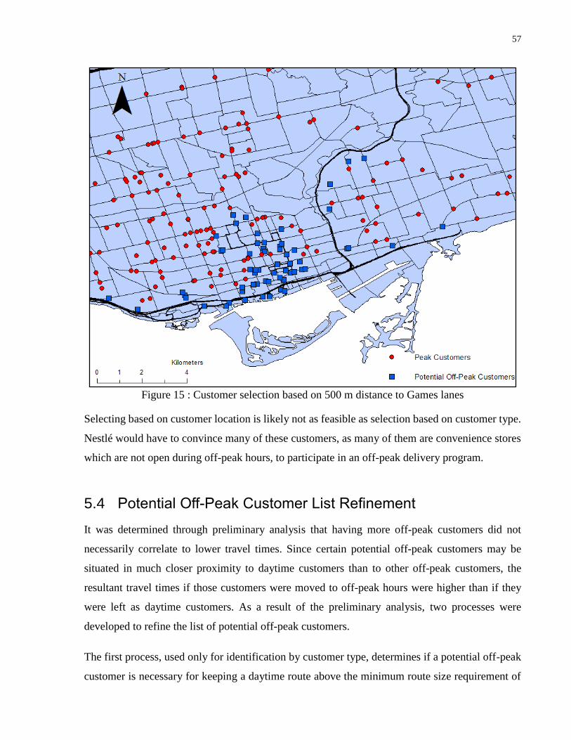
57
Figure 15 : Customer selection based on 500 m distance to Games lanes
Selecting based on customer location is likely not as feasible as selection based on customer type.
Nestlé would have to convince many of these customers, as many of them are convenience stores
which are not open during off-peak hours, to participate in an off-peak delivery program.
5.4 Potential Off-Peak Customer List Refinement
It was determined through preliminary analysis that having more off-peak customers did not
necessarily correlate to lower travel times. Since certain potential off-peak customers may be
situated in much closer proximity to daytime customers than to other off-peak customers, the
resultant travel times if those customers were moved to off-peak hours were higher than if they
were left as daytime customers. As a result of the preliminary analysis, two processes were
developed to refine the list of potential off-peak customers.
The first process, used only for identification by customer type, determines if a potential off-peak
customer is necessary for keeping a daytime route above the minimum route size requirement of

58
five customers. The second process adapts a clustering outlier algorithm to determine if a potential
off-peak customer is an outlier during the off-peak hours, and if there would be an improvement
in moving that customer to the daytime. The two processes are referred to as the cluster refinement
process and the outlier refinement process respectively. The outlier refinement process was used
for both selection by customer type and for selection by customer distance to the GRN. The cluster
refinement process was determined to not be a necessary addition for identification by customer
type, but was not required for identification by proximity to the GRN.
The algorithm for the cluster refinement process is presented in Figure 16. In broad terms it refines
the list of potential off-peak customers by determining if delivering to certain customers during
the off-peak hours would result in certain daytime routes falling below the minimum size
constraint. More specifically, the cluster refinement process starts by determining the optimal
clustering should all the customers be delivered to during the daytime. Then, for each of the
clusters generated, the total number of clusters being represented by the variable kmax, the number
of potential off-peak customers, nop, and the total number of customers, nk, contained in the cluster
is determined. If the difference between nk and nop is greater than five, the minimum route size
constraint, then the cluster in question contains enough daytime customers to create a route. If the
difference between nk and nop is less than five it must be determined whether there are sufficient
nearby clusters which may be joined with the cluster in question, bringing the total number of
customers above the minimum size constraint.
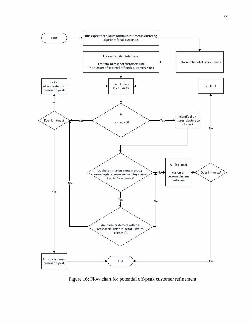
59
Figure 16: Flow chart for potential off-peak customer refinement
Start
End
Run capacity and route constrained k-means clustering algorithm for all customers
For each cluster determine:
The total number of customers = nk
The number of potential off-peak customers = nop
Is
nk - nop < 5?
For clusters k = 1 : kmax
YesIdentify the 4
closest clusters to cluster k
Do these 4 clusters contain enough extra daytime customers to bring cluster
k up to 5 customers?
Yes
Are those customers within a reasonable distance, set at 5 km, to
cluster k?
No
NoDoes k = kmax?
Does k = kmax?
Yes
Yes
No
5 – (nk - nop)
customers become daytime
customers
No
k = k+1All nop customers remain off-peak
All nop customersremain off-peak
Yes
No
k = k + 1
Total number of clusters = kmax

60
This concept is illustrated in Figure 17, which contains all of the customers for one scenario. The
square customers are the potential off-peak customers as identified by customer type, and the
remaining customers are daytime customers.
Figure 17: Example of the clustering refinement process
The customers, both potential off-peak and daytime, contained within the circle belong to one
route should all customers be delivered to during the daytime. If all the potential off-peak
customers were to remain as off-peak customers there would only be two daytime customers
remaining in that route, both of which are a large distance from any other daytime route.
The outlier refinement process identifies customers that have the potential to be serviced in the
off-peak hours, but that are more closely situated to daytime customers. The savings that could
potentially be made in the off-peak hours are negated by the longer distances the truck would have

61
to travel to reach these customers during the off-peak routes. The difference between the outlier
refinement process and the cluster refinement process (Figure 16) is that the cluster refinement
process identifies customers that are required to stay as daytime customers in order to ensure that
the daytime routes meet the minimum route size requirements, while the outlier refinement process
identifies customers that fit in better to daytime routes.
This outlier detection process is based on the work of Pamula et al. (2011). For each customer i,
an outlier number is generated based both on its proximity to other customers, di, as well as the
proximity of those other customers to each other, Di. Nq is the group of the w closest customers,
and q is one of the k customers in Nq.
𝑶𝒖𝒕𝒍𝒊𝒆𝒓𝒊 = 𝒅𝒊
𝑫𝒊
Equation 1
𝒅𝒊 =𝟏
𝒘∑ 𝒅𝒊𝒔𝒕(𝒊, 𝒒)
𝒒 ∈ 𝑵𝒒
Equation 2
𝑫𝒊 =𝟏
𝒘(𝟏 − 𝒘)∑ ∑ 𝒅𝒊𝒔𝒕(𝒒, 𝒒′)
𝒒′ ∈ 𝑵𝒒
𝒒≠𝒒′
𝒒 ∈ 𝑵𝒒
Equation 3
The larger the outlier number is, the more of an outlier that customer is in relation to nearby
customers. This means a customer’s average distance to nearby customers is larger than the
average distance of those customers to each other. No changes to the equations were made, but the
method in how they were used was altered to adapt it to the off-peak outlier scenario. This involved
calculating Outlieri twice for each customer, once using potential off-peak customers to generate
Nq, while the second time using both potential off-peak and daytime customers to generate Nq. The
number of nearby customers, w, was taken to be four. The reason four was chosen for w is that the
four closest customers, plus the customer in question, is five total customers, the same size as the
minimum route size constraint for a single truck. Using only potential off-peak customers
generates an outlier number for that customer for a potential off-peak route, while using daytime
customers generates a similar outlier number for potential daytime routes. The difference in these
two numbers indicates whether there would be improvement in travel times by keeping customer
i as a daytime customer over making it an off-peak customer.

62
If the difference between the daytime and off-peak outlier number exceeds a certain cutoff number
it is determined that the customer is better of left as a daytime customer. For selection by customer
type the cutoff number was determined empirically to be 20, and any difference between the
daytime and off-peak outlier numbers greater than 20 indicates that that customer should be left as
a daytime customer. Various cutoff numbers were tested, with smaller cutoffs resulting in too
many potential off-peak customers moved to the daytime, and numbers larger than 20 resulting in
too few. For selection by customer distance to the GRN, the cutoff number was determined to be
a lot smaller at only 0.5. The reason that these two cutoff numbers are so different reflects the
differences in where the off-peak customers are located. Selecting off-peak customers by type
results in a moderately even distribution of off-peak customers, whereas selecting by proximity to
the GRN will result in off-peak customers in much closer proximity to one another. A cutoff of
20 for selection by distance to the GRN will result in no refinement of the potential off-peak
customers. Figure 18 shows the outcome of this algorithm for selection by customer type.
Figure 18: Identifying outlying potential off-peak customers

63
5.5 Off-Peak Customer Selection
Once the list of potential off-peak customers has been refined, the next step in the heuristic is to
select off-peak customers for clustering. Two methods were tested for selecting off-peak customers
for different numbers of off-peak routes: random selection and strategic selection. The details of
each of these methods is presented in the following sections.
5.5.1 Random Customer Selection
Random customer selection reflects the possibility that Nestlé does not have control over which
customers would choose to participate in their off-peak delivery program. Customers would
choose to participate because they perceive some benefit to themselves, and not due to any
influence from Nestlé. The method randomly selects subsets of customers from the group of
potential off-peak customers without any of the refinement processes being applied to that list of
customers. The number of customers chosen depends on the number of trucks that are being
designated as off-peak trucks. For example, if two off-peak routes are designated, a sufficient
number of customers are identified such that their total demand does not exceed the capacity of
two trucks. The location of the customers had no influence as to which customers were selected.
The following flowchart, Figure 19, outlines the process of randomly selecting off-peak customers.
The inputs required are the demand quantity for each customer, qi, as well as the total number of
customers N. Customers are assigned a randomly generated number, and the order in which these
customers are assigned to the trucks depends on the number generated. The number of customers
assigned to the truck depends on the total demand the truck is carrying, qcurrent, and the number
of customers being delivered to, ncurrent. No further customers are assigned to a truck if either
qcurrent or ncurrent are going to be larger than the truck capacity, qmax, or the maximum route
size, nmax, respectively.

64
Figure 19: Random off-peak customer selection algorithm
Figure 20 and Figure 21 are two examples of the output of the random off-peak customer
selection
Start
End
Inputs
Demand Quantity for each customer = qi
Total number of customers = N
Initializeqcurrent = 0qmax = 960ncurrent=0nmax=22
Sort customers based on random
number from smallest to largest
Starting with customer i = 1
Is qi + qcurrent < qmax?
Yes
Is ncurrent+1 < nmax?
Yes
Assign customer i as an off-peak customer
qcurrent = qcurrent + qi
ncurrent = ncurrent +1
Does i = N?YesOutput group of
off-peak customers
Assign each customer a random
number between 0 -1
Noi = i+1No
No
i = i + 1

65
Figure 20: The output of random off-peak customer selection for one truck
Figure 21: The output of random off-peak customer selection for two trucks
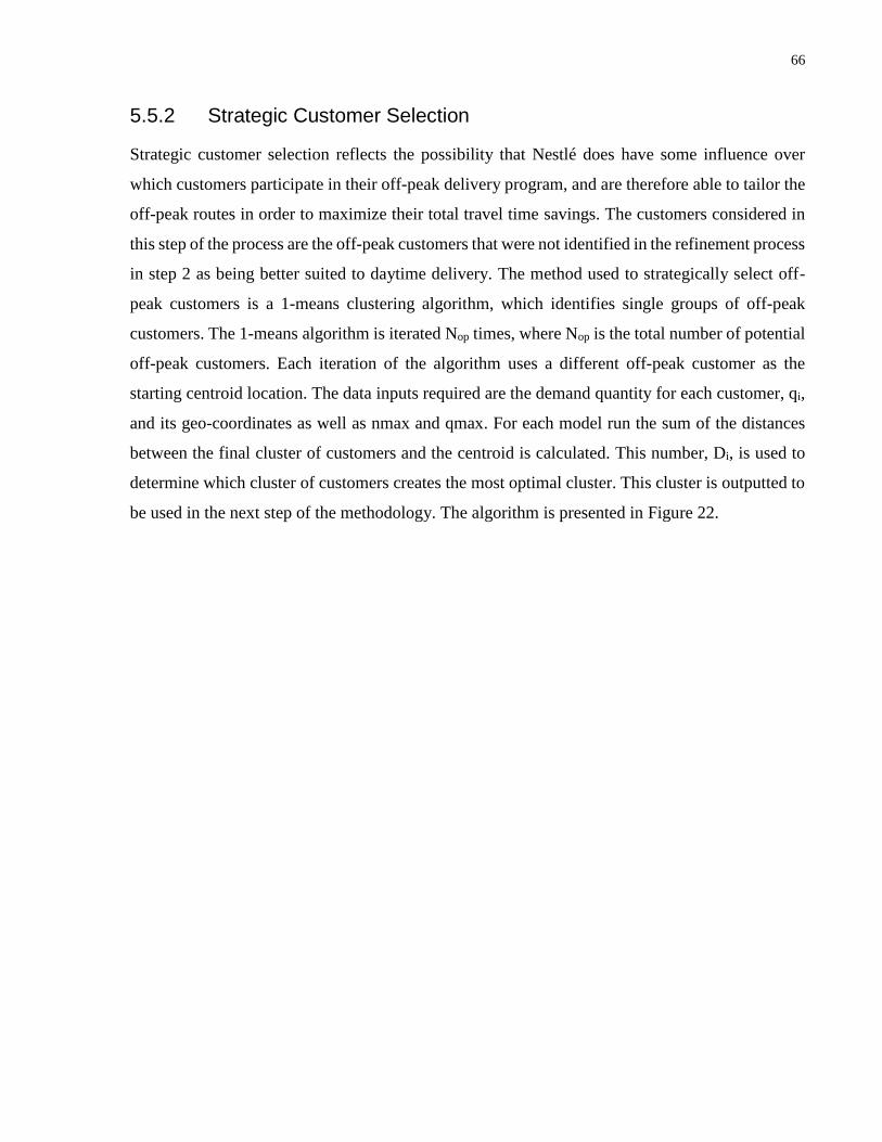
66
5.5.2 Strategic Customer Selection
Strategic customer selection reflects the possibility that Nestlé does have some influence over
which customers participate in their off-peak delivery program, and are therefore able to tailor the
off-peak routes in order to maximize their total travel time savings. The customers considered in
this step of the process are the off-peak customers that were not identified in the refinement process
in step 2 as being better suited to daytime delivery. The method used to strategically select off-
peak customers is a 1-means clustering algorithm, which identifies single groups of off-peak
customers. The 1-means algorithm is iterated Nop times, where Nop is the total number of potential
off-peak customers. Each iteration of the algorithm uses a different off-peak customer as the
starting centroid location. The data inputs required are the demand quantity for each customer, qi,
and its geo-coordinates as well as nmax and qmax. For each model run the sum of the distances
between the final cluster of customers and the centroid is calculated. This number, Di, is used to
determine which cluster of customers creates the most optimal cluster. This cluster is outputted to
be used in the next step of the methodology. The algorithm is presented in Figure 22.

67
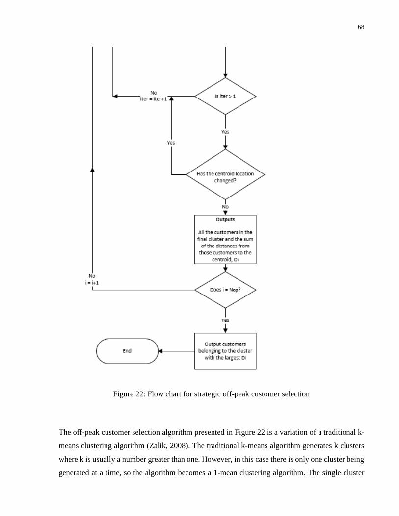
68
Figure 22: Flow chart for strategic off-peak customer selection
The off-peak customer selection algorithm presented in Figure 22 is a variation of a traditional k-
means clustering algorithm (Zalik, 2008). The traditional k-means algorithm generates k clusters
where k is usually a number greater than one. However, in this case there is only one cluster being
generated at a time, so the algorithm becomes a 1-mean clustering algorithm. The single cluster

69
generated represents one delivery truck which delivers to all the customers contained in that
cluster. The size of the cluster is limited by the same set of constraints introduced in the random
customer selection algorithm in the previous section of this thesis. The truck capacity constraint
limits the total demand of customers so that the sum of the total demand quantity of the customers
in the cluster does not exceed the carrying capacity of the truck.
The 1-means clustering problem is a relatively simple computational problem. The algorithm only
has to be run once for each customer in the pool of potential off-peak customers in order to find
the optimal solution. This is in contrast with a k-means algorithm where k is greater than one. For
that type of problem, to test every combination of starting centroid locations quickly becomes very
computationally intensive. The reason this was used for off-peak delivery customer selection is
that it can find single compact clusters out of the large number of potential clusters. This is
beneficial to Nestlé, who may only be able to offer incentives to a small number of customers,
which will in turn only generate a small number of off-peak routes. Figure 23 and Figure 24 provide
examples of the output of strategic off-peak customer selection.
Figure 23: The output of strategic off-peak customer selection for k=1.

70
Figure 24: The output of strategic off-peak customer selection for k=2.
5.6 Capacity Constrained K-Means Clustering
This section of the methodology involves grouping both the daytime and off-peak customers into
clusters. Each cluster of customers can then be serviced by one truck, either entirely in the daytime
or entirely in the off-peak hours. The clustering was done using a capacity constrained k-means
clustering algorithm. The algorithm groups customers into clusters with the objective of
minimizing the total distance between each customer and its associated cluster centroid. The size
of a cluster, meaning the number of customers assigned to it, is limited by the capacity of the truck
that will serve it, the number of stops one truck can reasonably make in a full 24-hrs, and the
minimum number of customers required for a route. These constraints are referred to as the
capacity constraint, the maximum route size constraint, and the minimum route size constraint
respectively. The formulation of the capacity constrained k-means clustering algorithm, and the
specifics of the constraints, are outlined below in Figure 25.
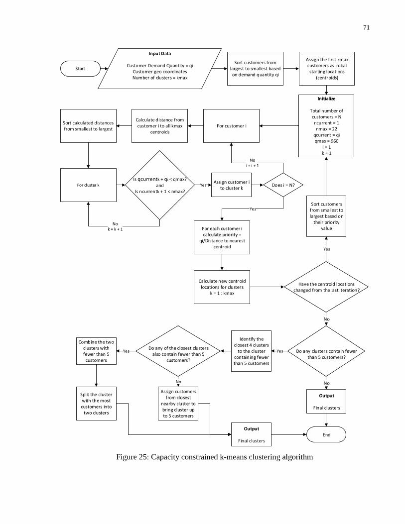
71
Figure 25: Capacity constrained k-means clustering algorithm
Start
Input Data
Customer Demand Quantity = qiCustomer geo coordinatesNumber of clusters = kmax
Initialize
Total number of customers = Nncurrent = 1nmax = 22
qcurrent = qi
qmax = 960i = 1k = 1
Sort customers from largest to smallest based on demand quantity qi
Assign the first kmax customers as initial starting locations
(centroids)
Calculate distance from customer i to all kmax
centroids
Sort calculated distances from smallest to largest
Is qcurrentk + qi < qmax?and
Is ncurrentk + 1 < nmax?
Assign customer i to cluster k
For customer i
For cluster k
Nok = k + 1
Yes Does i = N?
Noi = i + 1
For each customer i calculate priority =
qi/Distance to nearest centroid
Yes
Calculate new centroid locations for clusters
k = 1 : kmax
Have the centroid locations changed from the last iteration?
Yes
Sort customers from smallest to largest based on
their priority value
No
Do any clusters contain fewer than 5 customers?
End
Do any of the closest clusters also contain fewer than 5
customers?
Combine the two clusters with fewer than 5
customers
Split the cluster with the most customers into
two clusters
Identify the closest 4 clusters
to the cluster containing fewer than 5 customers
YesYes
No
Assign customers from closest
nearby cluster to bring cluster up to 5 customers
No
Output
Final clusters
Output
Final clusters

72
Geetha et al. (2009) incorporates two distinct alterations to a more traditional k-means clustering
algorithm (Zalik, 2008). The first alteration added a capacity constraint specifically designed to
incorporate truck capacity. This limited the size of the clusters so that the total demand from one
cluster would fit on one truck. The second alteration Geetha et al. (2009) made was the inclusion
of a priority assignment value. The k-means algorithm is an iterative process, meaning the optimal
solution is usually not found with the first customer assignment. Each iteration requires the
identification of the new centroid locations, and the process is repeated until these centroid
locations do not change between successive iterations. The priority value allows for a more
efficient customer assignment order. The priority value is a function of both the customer demand
quantity as well as the customers distance to the nearest centroid. The first benefit is that this
ensures that customers with large demands are not left until the end of the assignment order. The
reason this would be a problem is because it is likely that by the end of the customer assignment
process, many of the routes will be very near capacity in terms of total customer demand quantity
and the number of customers in that route. Therefore customers with large demands left to the end
of the assignment would have difficulty fitting into nearby routes. The priority function also
ensures that customers with small orders, but that are situated very close to a centroid, are also
assigned earlier. This limits the scenario where a customer that is very close to a cluster centroid
cannot join that cluster due to the capacity and route size constraints.
There are several practical improvements on the Geetha et al. (2009) method which are introduced
in this project. These improvements are the addition of constraints which limit the size, being the
number of customers, in a cluster. The maximum and minimum route size constraints are based
upon the delivery limits taken from the Nestlé delivery logs presented in section 4.3.2.
There are some challenges to using a k-means style clustering algorithm. For example, it is possible
for the algorithm to get stuck in a loop, alternating between local minima. This occurs when one
set of centroid locations is identified in one iteration, and in the next iteration there is a small shift
in customer allocation resulting in a slightly different set of centroid locations. The iteration after
that can revert back to the previous group of centroid locations, and this process will repeat itself
endlessly. If this is the case changing the initial centroid locations can sometimes result in the
algorithm converging properly. The process of changing the starting conditions, in this case the
initial centroid locations, is an adaptation of work conducted by Bradley and Fayyad (1998) and
Bradley et al. (2000). This method is also used to attempt to eliminate clusters with fewer than five

73
customers. Exchanging the initial centroid which results in a cluster with fewer customers than the
minimum required allows the model to re-run, potentially resulting in the elimination of the cluster
in question.
If changing the initial centroid locations still results in a cluster with fewer than five customers, a
second step must be taken. This step involves assigning customers from nearby clusters to the
smallest cluster in order for it to meet the minimum size requirements. This results in a slightly
less optimal solution, due to the fact that some customers have to be reassigned, but maintains the
number of trucks used and ensures all the trucks have a least the minimum number of customers
assigned to them, and no more than the maximum allowed. It is important to note that customers
are only reassigned if their reassignment does not in turn result in the violation of the minimum
capacity constraint of the cluster they are being assigned from.
5.7 Vehicle Routing
The final step in the process is a vehicle routing algorithm. The single vehicle routing problem is
formulated as a binary integer linear program. The algorithm is adapted primarily from Laporte
(1992) and Winkenbach et al. (2012). Laporte (1992) provides a summary of exact and heuristic
solution methods for the vehicle routing problem. The bulk of the formulation for the vehicle
routing problem is taken from Laporte (1992) while the detail on integer linear programming is
provided by Winkenbach et al. (2012).
The algorithm inputs required are: f, tij, ni, V, and S. The objective function to be minimized, f, is
the total travel time for the truck to visit all of the customers, and is a function of tij and xij. The
travel time, tij, is the travel time between customer i and customer j. The binary decision variable
xij is a is equal to one if the truck travels from customer i to customer j, or is equal to zero if the
truck does not travel from customer i to customer j. The variable ni is the number of customers,
including customer i, that are located in the same zone as customer i. V is a matrix which is used
for the subtour elimination constraint. Each row of the matrix V contains a different combination
of the customers being routed, and as a whole V contains every possible combination of customers
for the given routing problem. Every possible subtour is therefore contained somewhere within the
matrix V. S is a subset of the matrix V, and represents one possible subtour contained within the
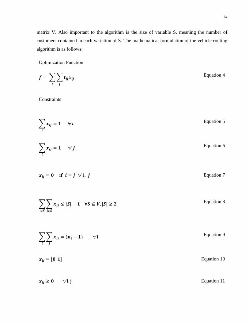
74
matrix V. Also important to the algorithm is the size of variable S, meaning the number of
customers contained in each variation of S. The mathematical formulation of the vehicle routing
algorithm is as follows:
Optimization Function
𝒇 = ∑ ∑ 𝒕𝒊𝒋𝒙𝒊𝒋
𝒋𝒊
Equation 4
Constraints
∑ 𝒙𝒊𝒋
𝒋
= 𝟏 ⍱𝒊 Equation 5
∑ 𝒙𝒊𝒋
𝒊
= 𝟏 ⍱ 𝒋 Equation 6
𝒙𝒊𝒋 = 𝟎 𝐢𝐟 𝒊 = 𝒋 ⍱ 𝐢, 𝒋 Equation 7
∑ ∑ 𝒙𝒊𝒋
j∈𝑺
≤ |𝑺| − 𝟏 ∀𝑺 ⊆ 𝑽, |𝑺| ≥ 𝟐
i∈𝑺
Equation 8
∑ ∑ 𝒙𝒊𝒋 = (𝒏𝒊 − 𝟏)
𝒋𝒊
⍱𝐢 Equation 9
𝒙𝒊𝒋 = [𝟎, 𝟏] Equation 10
𝒙𝒊𝒋 ≥ 𝟎 ⍱𝐢, 𝐣 Equation 11

75
The objective function, Equation 4, is the total vehicle routing travel time. The objective is to
minimize the function f without violating any of the other constraints. Equation 5 and Equation 6
ensure that the truck only arrives at and only leaves each customer one time. Equation 7 ensures
that customer i and customer j are not the same, making sure that every trip made is between
different customers. Equation 8 is the subtour elimination constraint, which is discussed in more
detail in section 5.7.1. Equation 9 is a constraint that forces all customers located in the same zone
to be linked in such a way that the truck delivers to all these customers before leaving the zone.
Further details and reasoning are also discussed in section 5.7.1. Equation 10 is the binary
constraint, which limits the value of xij to either zero or one. Finally, Equation 11 is the non-
negativity constraint.
The program used to solve the linear program is a simplex-based solver called IBM ILOG CPLEX.
A CPLEX plugin created by IBM for Matlab was used for this project. Generation of the objective
function and constraints was done in Matlab, which in turn were used as inputs into the CPLEX
plugin. This method takes advantage of Matlab’s simple user interface as well as CPLEX’s
efficient linear program solver.
5.7.1 Subtour Elimination
The subtour elimination constraint is the most computationally intensive component of the
optimization algorithm. The method employed does not create constraints for every possible
subtour due to the immense number of subtour combinations possible. For example, there are over
500,000 ways to create different combinations of customers from a 20 customer tour, which means
there are over 500,000 different possible subtours that can be created. Generating these matrices
is too computationally intensive for Matlab. However, constraints for subtours containing two,
three, and four customers are within the capabilities of Matlab and were therefore generated
beforehand. Eliminating the smaller subtours (two, three, and four stops) prior to solving the
vehicle routing algorithm reduces the computational time required.
After the CPLEX plugin solves the linear program, a check is made to identify any subtours in the
solution vector. This is done by examining the solution vector to see if all the customers are visited
in one continuous tour before the truck returns to the depot. Returning to the depot before

76
delivering to every customer indicates that there are at least two subtours present in the solution
vector, and that the calculated solution vector is not a viable solution. If this happens, specific
constraints are added to the linear program for the next iteration according to Equation 8. These
constraints are formulated so that the specific subtours identified do not appear in the solution
vector x during the next iteration (Laporte et al, 2006). This process of solving the linear program,
identifying subtours in the solution vector, creating specific constraints to eliminate those subtours,
and rerunning the algorithm is repeated until the solution vector x contains no subtours.
The long model run time is a result of the problem formulation and the subtour elimination
constraints. Travel time data is not available between all customers’ actual locations, so zonal
travel times are used as a reasonable approximation. An issue arises when multiple customers are
located within the same zone. With multiple customers in the same zone, there now exist multiple
subtour possibilities, all of which contain the same travel time. Figure 26 below provides an
example of multiple subtours within a group of four zones. The ideal solution for the customers in
Figure 26 would be to have one tour which begins and ends at customer one, and that visits every
other customer. Instead, the solution presented contains two subtours; smaller tours which do not
visit every customer. Both of the two subtours illustrated have the same travel time according to
the zonal travel time method. The reason this is such a significant issue in terms of computational
time is due to the number of subtour combinations available. For example, there exist 16 different
ways to connect one customer from each zone in Figure 26. For more complex problems, the
number of subtours gets exponentially larger. The problem is still solvable, but for each time
constraint that is added, the longer the CPLEX solver takes to solve the linear program.
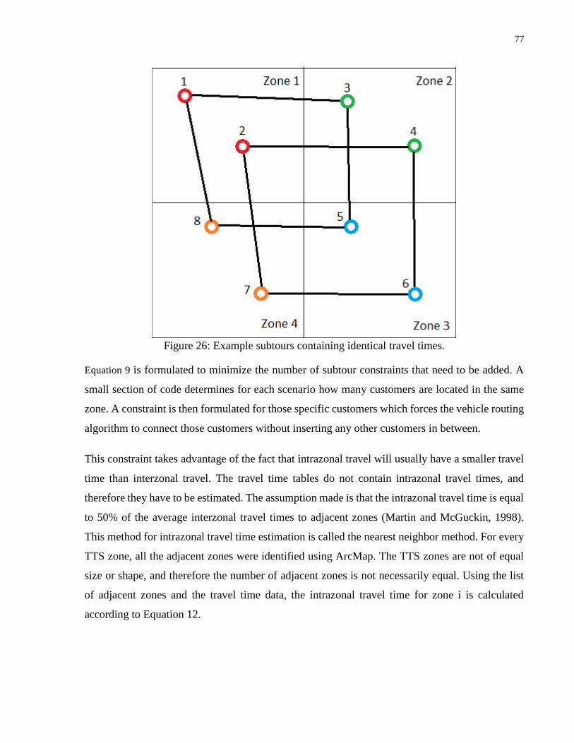
77
Figure 26: Example subtours containing identical travel times.
Equation 9 is formulated to minimize the number of subtour constraints that need to be added. A
small section of code determines for each scenario how many customers are located in the same
zone. A constraint is then formulated for those specific customers which forces the vehicle routing
algorithm to connect those customers without inserting any other customers in between.
This constraint takes advantage of the fact that intrazonal travel will usually have a smaller travel
time than interzonal travel. The travel time tables do not contain intrazonal travel times, and
therefore they have to be estimated. The assumption made is that the intrazonal travel time is equal
to 50% of the average interzonal travel times to adjacent zones (Martin and McGuckin, 1998).
This method for intrazonal travel time estimation is called the nearest neighbor method. For every
TTS zone, all the adjacent zones were identified using ArcMap. The TTS zones are not of equal
size or shape, and therefore the number of adjacent zones is not necessarily equal. Using the list
of adjacent zones and the travel time data, the intrazonal travel time for zone i is calculated
according to Equation 12.
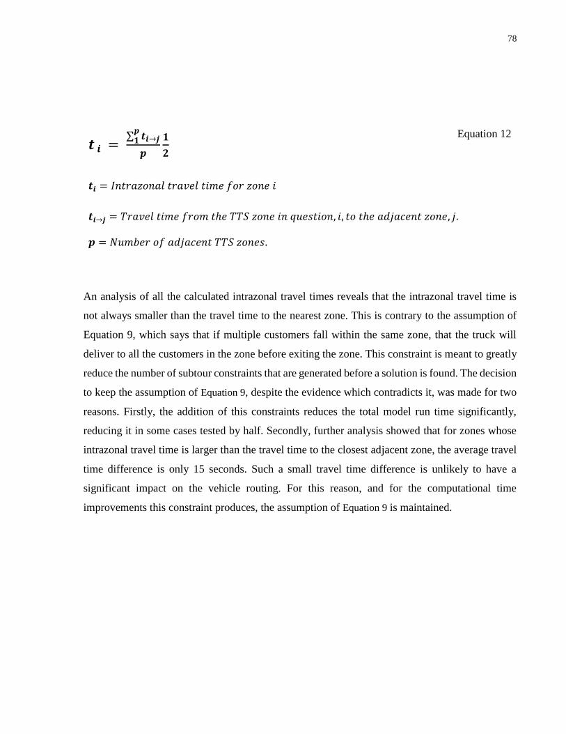
78
𝒕 𝒊 = ∑ 𝒕𝒊→𝒋
𝒑𝟏
𝒑
𝟏
𝟐
Equation 12
𝒕𝒊 = 𝐼𝑛𝑡𝑟𝑎𝑧𝑜𝑛𝑎𝑙 𝑡𝑟𝑎𝑣𝑒𝑙 𝑡𝑖𝑚𝑒 𝑓𝑜𝑟 𝑧𝑜𝑛𝑒 𝑖
𝒕𝒊→𝒋 = 𝑇𝑟𝑎𝑣𝑒𝑙 𝑡𝑖𝑚𝑒 𝑓𝑟𝑜𝑚 𝑡ℎ𝑒 𝑇𝑇𝑆 𝑧𝑜𝑛𝑒 𝑖𝑛 𝑞𝑢𝑒𝑠𝑡𝑖𝑜𝑛, 𝑖, 𝑡𝑜 𝑡ℎ𝑒 𝑎𝑑𝑗𝑎𝑐𝑒𝑛𝑡 𝑧𝑜𝑛𝑒, 𝑗.
𝒑 = 𝑁𝑢𝑚𝑏𝑒𝑟 𝑜𝑓 𝑎𝑑𝑗𝑎𝑐𝑒𝑛𝑡 𝑇𝑇𝑆 𝑧𝑜𝑛𝑒𝑠.
An analysis of all the calculated intrazonal travel times reveals that the intrazonal travel time is
not always smaller than the travel time to the nearest zone. This is contrary to the assumption of
Equation 9, which says that if multiple customers fall within the same zone, that the truck will
deliver to all the customers in the zone before exiting the zone. This constraint is meant to greatly
reduce the number of subtour constraints that are generated before a solution is found. The decision
to keep the assumption of Equation 9, despite the evidence which contradicts it, was made for two
reasons. Firstly, the addition of this constraints reduces the total model run time significantly,
reducing it in some cases tested by half. Secondly, further analysis showed that for zones whose
intrazonal travel time is larger than the travel time to the closest adjacent zone, the average travel
time difference is only 15 seconds. Such a small travel time difference is unlikely to have a
significant impact on the vehicle routing. For this reason, and for the computational time
improvements this constraint produces, the assumption of Equation 9 is maintained.

79
Chapter 6
Results and Discussion
This chapter introduces the scenario analyses used for this project and presents the results of the
quantitative analysis for the Nestlé case study. The purpose of the quantitative aspect of this
research was to determine the travel time impacts large sporting events like the Pan Am Games
can have on a company’s day-to-day operations, as well whether off-peak delivery can be used to
mitigate some of these impacts and result in decreased overall travel times. The four research
questions examined were:
1. What will be the impact of the Pan Am Games on current Nestlé operations?
2. What are the benefits of planning routes one week at a time rather than on a call-and-place
basis for normal Nestlé operations outside of the Games?
3. Can off-peak delivery be used to mitigate the impacts from the Games?
4. Can advanced routing and off-peak delivery be used to reduce the total number of trucks
required?
6.1 Scenario Analysis
Nestlé has provided delivery log data for a portion of their deliveries between January and April
2014. The delivery data is separated into nine scenarios for analysis, with each scenario
representing a week’s worth of deliveries. The number of customers in each scenario, as well as
the number of potential off-peak customers, are presented in Table 3.

80
Table 3: Number of customers and summary of the number of potential off-peak customers for
all scenarios
Scenario
Total
Number of
Customers
Potential Off-Peak
Customers Identified
by Customer Type
Potential Off-Peak
Customers Identified
by Proximity to the
GRN
Number of
Routes Used by
Nestlé to Deliver
to All Customers
Number Percentage Number Percentage
1 235 76 32.3 60 25.5 20
2 137 28 20.4 62 45.3 15
3 161 38 23.6 61 37.9 14
4 192 48 25.0 50 26.0 18
5 211 70 33.2 55 26.1 19
6 172 62 36.0 46 26.7 16
7 249 84 33.7 51 20.5 25
8 173 50 28.9 50 28.9 17
9 145 52 35.9 41 28.3 14
The average number of customers for the nine scenarios was 180 customers, with an average of
56.4 potential off-peak customers when identified by customer type, 52.8 potential off-peak
customers when identified by proximity to the GRN, and delivered to by Nestlé by an average of
17.5 trucks.

81
6.2 Impact of the Pan Am Games on Nestlé’s Normal Operations
This section will outline the travel time impacts of the Pan Am Games on Nestlé’s normal
operations. This analysis estimates the increase in total travel time that Nestlé vehicles can expect
due to the impacts from the Pan Am Games should Nestlé not make any changes to their operations
in preparation for the Games. This analysis was performed using the delivery logs provided by
Nestlé and the travel time estimates provided by IBI Group. In order to estimate the impact of the
Games, two different travel time estimates were made. The Games travel times, which
incorporated the additional demand and the changes to the road network, and the BAU travel times,
which estimates the travel times without any of the changes due to the Games, were compared in
order to determine how much longer each trip would take. This is possible because the delivery
logs provided by Nestlé contain the order in which the customers were delivered to. This order of
customers was maintained for both the Games and BAU travel time scenarios in order to compare
the results. The results of this analysis are presented in Figure 27.
Figure 27: Total travel time comparison between Games and BAU conditions
0
500
1000
1500
2000
2500
3000
3500
4000
4500
1 2 3 4 5 6 7 8 9
Tota
l Tra
vel T
ime
(min
ute
s)
Scenario
GamesTravelTimes
BAUTravelTimes
82
The results in Figure 27 show higher travel times for the Games conditions compared against the
BAU conditions. The average travel time for Games conditions is approximately 6.4% higher than
the BAU, which corresponds to an average of 171 minutes of extra time spent on the road for a
one week period. This analysis only captures the travel time impacts, which are only one part of
the delivery process. Nestlé can expect further impacts from the Games in terms of parking search
time, especially around the GRN.
6.3 Impact of Advanced Routing on Travel Times
Current Nestlé delivery operations are organized on a call-and-place delivery model. Customers
will request deliveries somewhere between 24 and 48 hours in advance of when the delivery will
actually take place. The benefit of this method is that it provides flexibility for customers at the
expense of less efficient routes. The argument for more advanced routing is two-fold. Firstly,
planning deliveries in advance allows for a more optimal route generation, likely with much shorter
distances between stops. Secondly, a successful off-peak delivery program would require
advanced knowledge of which customers would be willing to accept off-peak delivery. It is
unlikely that a sufficient number of off-peak customers would be identified using the call-and-
place method to justify a complete off-peak route.
Table 4 shows the travel times generated for each scenario. For the call-and-place method the same
order of deliveries was maintained as was presented in the driver deliver logs. Each scenario,
roughly a week’s worth of customers, was then clustered using the capacity constrained k-means
clustering algorithm and routed using the vehicle routing algorithm. The travel times used were
the BAU travel times with all customers being delivered to during the daytime.
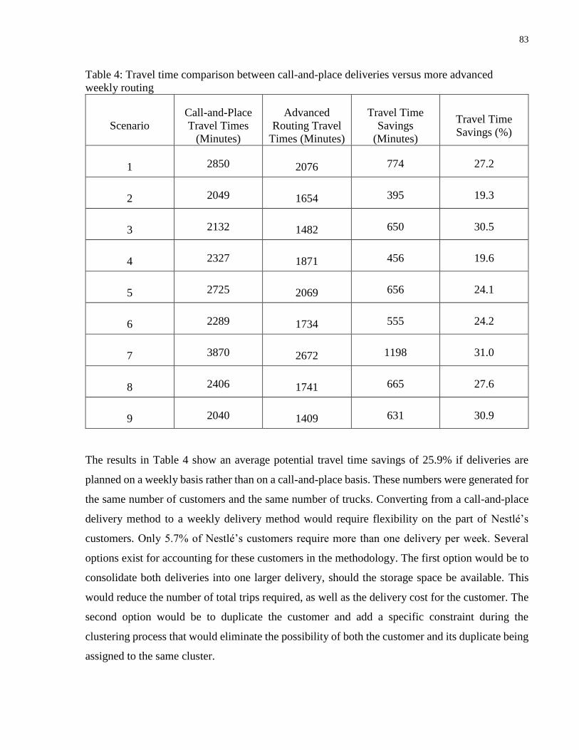
83
Table 4: Travel time comparison between call-and-place deliveries versus more advanced
weekly routing
Scenario
Call-and-Place
Travel Times
(Minutes)
Advanced
Routing Travel
Times (Minutes)
Travel Time
Savings
(Minutes)
Travel Time
Savings (%)
1 2850 2076 774 27.2
2 2049 1654 395 19.3
3 2132 1482 650 30.5
4 2327 1871 456 19.6
5 2725 2069 656 24.1
6 2289 1734 555 24.2
7 3870 2672 1198 31.0
8 2406 1741 665 27.6
9 2040 1409 631 30.9
The results in Table 4 show an average potential travel time savings of 25.9% if deliveries are
planned on a weekly basis rather than on a call-and-place basis. These numbers were generated for
the same number of customers and the same number of trucks. Converting from a call-and-place
delivery method to a weekly delivery method would require flexibility on the part of Nestlé’s
customers. Only 5.7% of Nestlé’s customers require more than one delivery per week. Several
options exist for accounting for these customers in the methodology. The first option would be to
consolidate both deliveries into one larger delivery, should the storage space be available. This
would reduce the number of total trips required, as well as the delivery cost for the customer. The
second option would be to duplicate the customer and add a specific constraint during the
clustering process that would eliminate the possibility of both the customer and its duplicate being
assigned to the same cluster.
84
6.4 Impact of Off-Peak Delivery on Travel Times during the Pan Am Games
The third quantitative thesis question analyzed the use of off-peak delivery in reducing travel times
during the Pan Am Games. The five step heuristic used for the analysis of this question was
presented in section 5.2 to 5.7 of this thesis. The first step identified potential off-peak customers
based either on their type or on their proximity to the GRN. The second step refined the list of
potential off-peak customers using combinations of two refinement processes referred to as the
cluster refinement process or the outlier refinement process. The refinement processes were only
used for strategic selection, as the random customer selection selected off-peak customers from
the complete list of potential off-peak customers. The third step selected off-peak customers from
the refined list either through random or strategic selection. The number of customers chosen for
off-peak delivery depended on the number of trucks being routed. A capacity constrained k-means
clustering algorithm was then used to separate the customers into different routes, or trucks, and
finally a vehicle routing algorithm was used to estimate travel times for each route.
In order to provide a basis for comparison of the results, the upper and lower limits for travel time
were determined by assigning all customers to the daytime or off-peak hours respectively. The all
daytime travel time analysis represents the total travel time should all customers be serviced in the
daytime hours, and provides the base travel time for which improvements can be compared. The
all off-peak analysis shows the very lowest travel times possible should all customers be delivered
to at night. The travel time tables used were the Pan Am Games scenario daytime tables and the
Pan Am Games scenario off-peak table. The results are presented in Table 5.

85
Table 5: Travel time results for all daytime and all off-peak customers
Scenario Number of
Clusters
Number of
Customers
Total Travel Time
All Daytime
Customers
(minutes)
Total Travel
Time All Off-
Peak Customers
(minutes)
Percentage
Travel Time
Decrease
1 20 235 2242 1653 26.3
2 15 137 1822 1312 28.0
3 14 161 1607 1194 25.7
4 18 192 2028 1489 26.6
5 19 211 2212 1656 25.1
6 16 172 1851 1390 24.9
7 25 249 2858 2112 26.1
8 17 173 1886 1395 26.0
9 14 145 1512 1125 25.6
The results in Table 5 show an average decrease in travel time of 26% between the all daytime and
all off-peak scenarios. These results represent the possibility for travel time improvements should
Nestlé’s entire delivery operations be shifted to off-peak hours. However, the likelihood that all of
Nestlé’s customers would participate in an off-peak delivery program is small. The rest of this
section (6.4) presents the results for the two potential off-peak identification methods, selection by
customer type and selection by customer proximity to the GRN, as well as the two methods of off-
peak customer selection, random selection and strategic selection.
Detailed results and figures are presented for scenario 1 in order to provide detail into how the
process works, and summarized results are presented for the remaining scenarios. Scenario 1 has
235 total customers, of which 76 are considered as potential off-peak customers according to their
customer type, and 60 are considered as potential off-peak customers according to their proximity
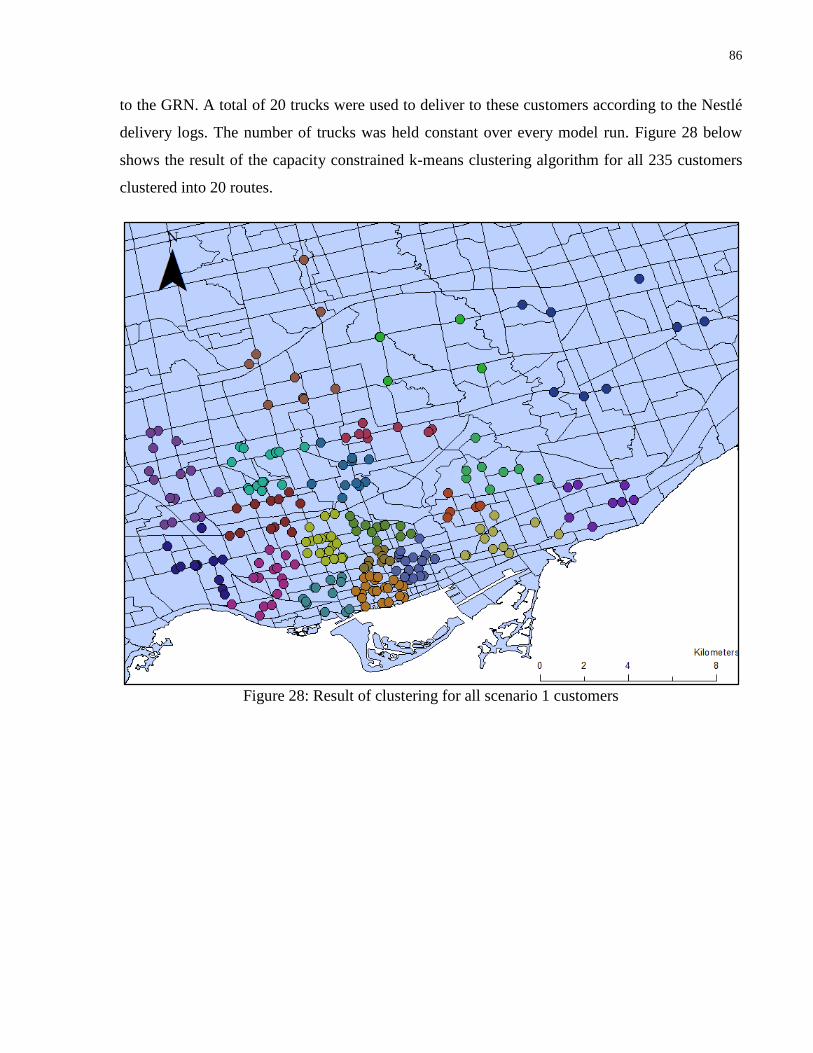
86
to the GRN. A total of 20 trucks were used to deliver to these customers according to the Nestlé
delivery logs. The number of trucks was held constant over every model run. Figure 28 below
shows the result of the capacity constrained k-means clustering algorithm for all 235 customers
clustered into 20 routes.
Figure 28: Result of clustering for all scenario 1 customers

87
6.4.1 Random Off-Peak Customer Selection
Random selection represents the possibility that Nestlé does not influence which potential off-peak
customers will participate in the off-peak delivery program, and instead participation will be purely
on a volunteer basis. The five-step heuristic is used for random selection, with the exception that
the second step, the refinement of the list of potential off-peak customers, is excluded. The analysis
presented in this section will show the travel time difference for off-peak routes created using
randomly selected off-peak customers. Table 6 and Table 7 show the travel time results for
randomly selected off-peak customers for identification by customer type and identification by
proximity to the GRN respectively for scenario 1. Complete results for the remaining 8 scenarios
can be found in the Appendix A.
Table 6: Travel times for randomly selected off-peak routes as identified by customer type
Number of
Off-Peak
Clusters
Number
of Peak
Clusters
Number of
Off-Peak
Customers
Number of
Peak
Customers
% of Off-
Peak
Customers
Total Travel
Time
(minutes)
All Daytime 0 20 0 235 0 2242
All Off-
Peak 20 0 235 0 100 1650
Selection by
Customer
Type
2 18 21 214 8.9 2224
Selection by
Customer
Type
3 17 42 193 17.9 2263
Selection by
Customer
Type
4 16 64 171 27.2 2233
Selection by
Customer
Type
5 15 76 159 32.3 2183
These results (Table 6) show that the travel times for randomly selecting off-peak customers may
result in higher travel times than if all customers were delivered to during the daytime. A travel

88
time decrease of 2.6% was the largest travel time decrease generated for five off-peak routes, an
increase in travel time of 0.9% was generated for three off-peak routes.
The results in Table 7 show the travel times for randomly selected off-peak customers identified
by proximity to the GRN.
Table 7: Travel times Travel times for randomly selected off-peak routes as identified by
proximity to the GRN.
Number of
Off-Peak
Clusters
Number
of Peak
Clusters
Number of
Off-Peak
Customers
Number of
Peak
Customers
% of Off-
Peak
Customers
Total Travel
Time
(minutes)
All Daytime 0 20 0 235 0 2242
All Off-
Peak 20 0 235 0 100 1650
Selection by
proximity to
GRN
2 18 22 213 9.4 2184
Selection by
proximity to
GRN
3 17 44 191 18.7 2168
Selection by
proximity to
GRN
4 16 60 175 25.5 2156
The results in Table 7 show travel time improvements for off-peak customers identified by
proximity to the GRN, up to 3.8%. When selecting off-peak customers based on the proximity to
the GRN, the resultant customers identified are all located within close proximity to one another.
This is not the case for potential off-peak customers identified by type, as those customers are
more evenly distributed across the city. For identification by customer type this means any travel
time benefits gained as a result of the off-peak delivery are negated by the extra distances needed
to travel between these more spread out customers. The differences between the two identification
methods can be seen in Figure 29
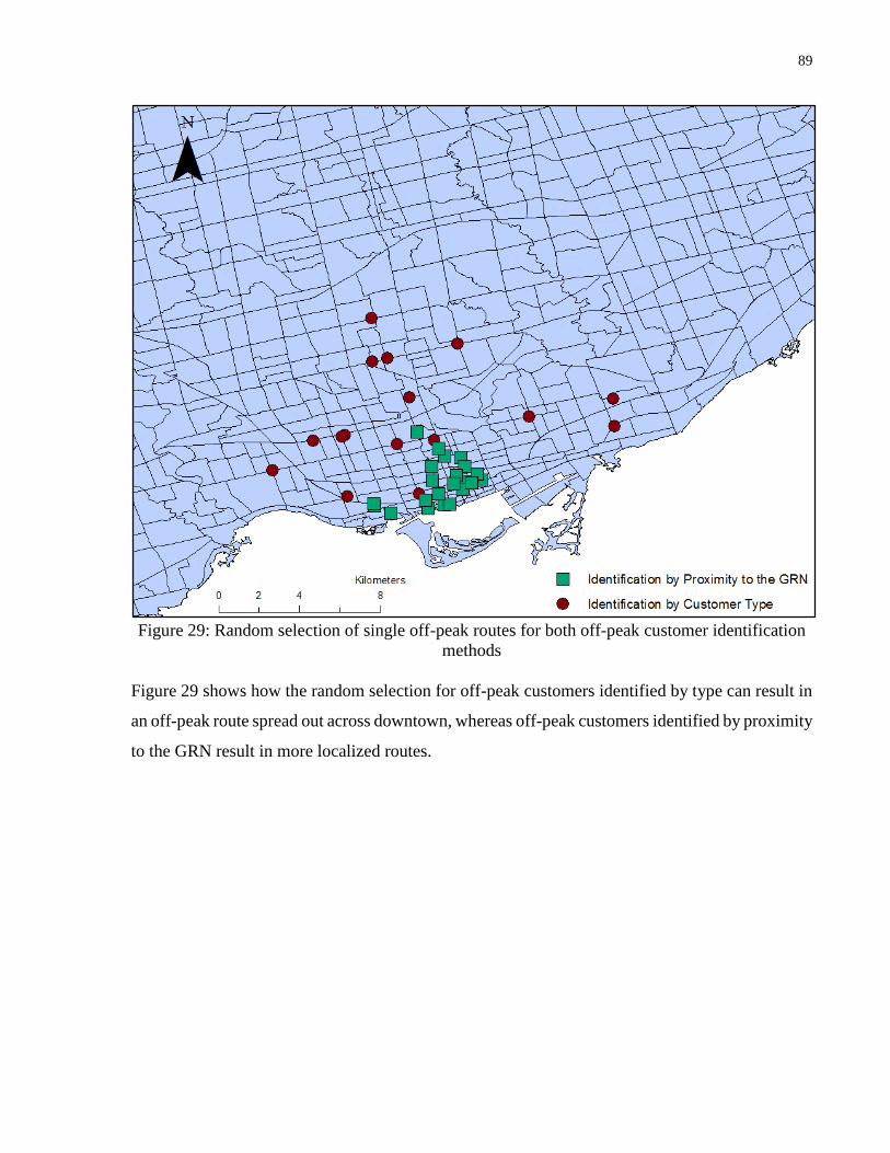
89
Figure 29: Random selection of single off-peak routes for both off-peak customer identification
methods
Figure 29 shows how the random selection for off-peak customers identified by type can result in
an off-peak route spread out across downtown, whereas off-peak customers identified by proximity
to the GRN result in more localized routes.

90
6.4.2 Strategic Selection by Customer Type
Strategic selection selects off-peak customers after the refinement processes have been applied to
the complete list of potential off-peak customers. Identification by customer type identifies
customers that may be more willing to accept off-peak delivery due to the fact that they already
operate in some capacity during the off-peak hours. The additional cost to these customers to
accept off-peak deliveries would likely be very low, or even zero. The benefit of identifying these
customers is that receiver participation is widely recognized as the principle barrier preventing the
implementation of off-peak delivery programs. Focusing on those customers that wouldn’t have
to incur large additional costs to accept off-peak deliveries would likely allow for more successful
off-peak program implementation. The potential off-peak customers for scenario 1 are shown in
Figure 30.
Figure 30: Potential off-peak customers for scenario 1 as identified by customer type

91
Figure 30 shows the distribution of the potential off-peak customers (grocery stores, department
stores, drug stores, and other 24-hr stores) are distributed evenly across the downtown core. Table
8 contains the results for total travel times for scenario 1 using different combinations the
refinement processes which refine the list of potential off-peak customers. The purpose of this
analysis is to show the benefits of using these refinement processes, rather than using all of the
potential off-peak customers. The shaded row in the different tables indicates the lowest travel
times.
Table 8: Travel time results for strategic selection by customer type for scenario 1.
Number
of Off-
Peak
Clusters
Number
of Peak
Clusters
Number
of Off-
Peak
Customers
Number
of Peak
Customers
% of Off-
Peak
Customers
Total Travel
Time
(minutes)
All Daytime 0 20 0 235 0 2242
All Off-Peak 20 0 235 0 100 1650
No Refinement
to List of
Potential Off-
Peak Customers
5 15 76 159 32.3 2161
Clustering Off-
Peak
Refinement
Only
5 15 73 162 31.1 2195
Outlier Off-Peak
Refinement
Only
5 15 65 170 27.6 2135
Both
Refinement
Processes
5 15 63 172 26.8 2100
The results in Table 8 show the total travel time improvements for delivering to all customers
during the off-peak hours, and the possible improvements incorporating the different refinement

92
processes. The maximum improvement in travel time possible by delivering to all customers
during the off-peak hours is 592 minutes. This represents a possible savings of 26.5% from the
case where all customers are delivered to during the daytime. The possible improvement made
delivering to all potential off-peak customers, without any refinement process is 81 minutes, a
3.6% travel time savings. The travel time after using the clustering refinement process is at 2195
minutes, while the outlier refinement process shows further improvement down to 2135 minutes.
When both processes are used, the travel time is reduced to 2100 minutes, a savings of 142 minutes
or 6.3%.
Table 9 contains the full set of results using different numbers of off-peak routes. The off-peak
customer selection algorithm strategically selected different numbers of off-peak customers
depending on the number of routes specified. Both refinement processes were used while
generating the results in Table 9.
Table 9: Comparison of travel times for different number of off-peak routes for scenario 1
Number of
Off-Peak
Clusters
Number
of Peak
Clusters
Number of
Off-Peak
Customers
Number of
Peak
Customers
% of Off-
Peak
Customers
Total Travel
Time
(minutes)
All Daytime 0 20 0 235 0 2242
All Off-
Peak 20 0 235 0 100 1650
Selection by
Customer
Type
2 18 20 215 8.5 2206
Selection by
Customer
Type
3 17 34 201 17.4 2155
Selection by
Customer
Type
4 16 56 179 24.7 2137
Selection by
Customer
Type
5 15 63 172 26.8 2100

93
Table 9 shows decreases in travel times for additional off-peak routes, with small expected
decreases for a single off-peak route, and larger expected decreases for the maximum number of
off-peak routes.
6.4.3 Strategic Selection by Proximity to the GRN
The same analysis was performed using off-peak customer identification by proximity to the GRN
as the method for identifying potential off-peak customers. There were 60 customers located
within the 500 m buffer to the GRN for scenario 1 out of the total 235 customers. Figure 31 shows
the location of the potential off-peak customers as identified by proximity to the GRN and Table
10 presents the travel time results using different combinations of the refinement processes.
Figure 31: Potential off-peak customers as identified by proximity to the GRN

94
The customers identified as potential off-peak customers in Figure 31 were not necessarily all
delivered to during off-peak hours. The refinement processes were applied to the list of potential
off-peak customers and the effectiveness of the different refinement process in reducing travel
time are presented in Table 10.
Table 10: Travel time results for strategic selection by customer proximity to the GRN for
scenario 1.
Number
of Off-
Peak
Clusters
Number
of Peak
Clusters
Number
of Off-
Peak
Customers
Number
of Peak
Customers
% of Off-
Peak
Customers
Total Travel
Time
(minutes)
All Daytime 0 20 0 235 0 2242
All Off-Peak 20 0 235 0 100 1650
No Refinement
to list of
Potential Off-
Peak Customers
4 16 60 175 25.5 2156
Clustering Off-
Peak
Refinement
Only
3 17 41 194 17.4 2188
Outlier Off-Peak
Refinement
Only
4 16 48 187 20.4 2123
Both
Refinement
Processes
3 17 30 205 12.8 2160
The results in Table 10 show similar results to those in Table 8, with one key difference. Using
only the cluster refinement process resulted in increased travel times, 2188 from the no refinement
time of 2156 minutes, while using both processes resulted in a very small increase in travel times.
The two refinement processes identify customer configurations, with the cluster refinement
process more likely to identify potential off-peak customers in closer proximity to one another.

95
For the case of selection by proximity to the GRN, the off-peak customers identified are in much
closer proximity to one another. This resulted in too many of the potential off-peak customers
being re-designated as daytime customers, generating a travel time that is higher than the no
refinement travel time. The largest decrease in travel times came as the result of only using the
outlier off-peak refinement process, with a decrease down to 2123 minutes. Using the outlier
refinement process only, travel times are presented in Table 11 for different numbers of off-peak
routes.
Table 11: Comparison of travel times for different number of off-peak routes for scenario 1
selection by proximity to the GRN
Number of
Off-Peak
Clusters
Number
of Peak
Clusters
Number of
Off-Peak
Customers
Number of
Peak
Customers
% of Off-
Peak
Customers
Total Travel
Time
(minutes)
All Daytime 0 20 0 235 0 2242
All Off-
Peak 20 0 235 0 100 1650
Selection by
proximity to
GRN
2 18 22 213 9.4 2194
Selection by
proximity to
GRN
3 17 44 191 18.7 2144
Selection by
proximity to
GRN
4 16 48 187 20.4 2123
Table 11 shows a similar trend to the results presented in Table 9. The results show that there can
be travel time improvements made by delivering to any number of off-peak customers but
decreasing travel times as the number of off-peak routes increases. The results for the remaining
scenarios are presented in the Appendix A.
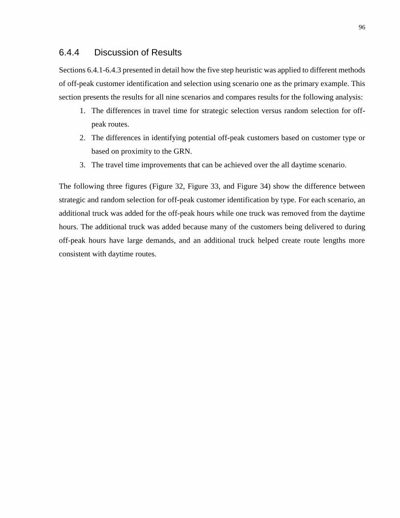
96
6.4.4 Discussion of Results
Sections 6.4.1-6.4.3 presented in detail how the five step heuristic was applied to different methods
of off-peak customer identification and selection using scenario one as the primary example. This
section presents the results for all nine scenarios and compares results for the following analysis:
1. The differences in travel time for strategic selection versus random selection for off-
peak routes.
2. The differences in identifying potential off-peak customers based on customer type or
based on proximity to the GRN.
3. The travel time improvements that can be achieved over the all daytime scenario.
The following three figures (Figure 32, Figure 33, and Figure 34) show the difference between
strategic and random selection for off-peak customer identification by type. For each scenario, an
additional truck was added for the off-peak hours while one truck was removed from the daytime
hours. The additional truck was added because many of the customers being delivered to during
off-peak hours have large demands, and an additional truck helped create route lengths more
consistent with daytime routes.
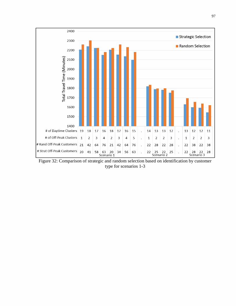
97
Figure 32: Comparison of strategic and random selection based on identification by customer
type for scenarios 1-3

98
Figure 33: Comparison of strategic and random selection based on identification by customer
type for scenarios 4-6
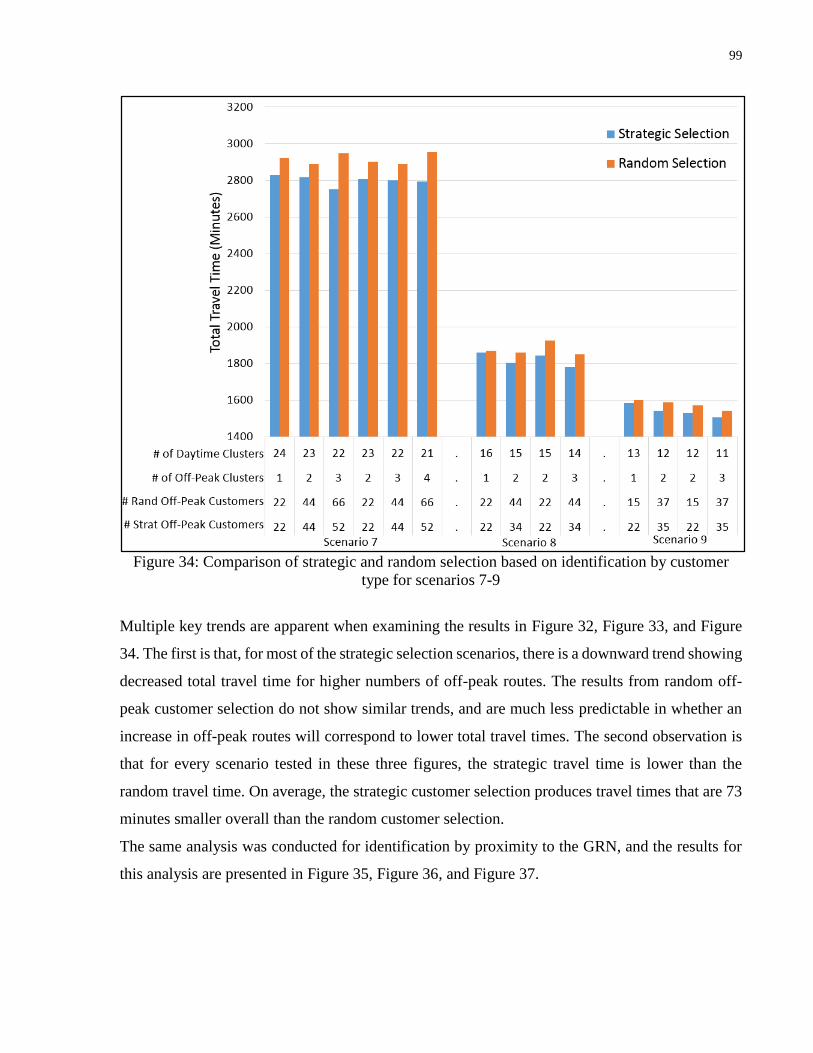
99
Figure 34: Comparison of strategic and random selection based on identification by customer
type for scenarios 7-9
Multiple key trends are apparent when examining the results in Figure 32, Figure 33, and Figure
34. The first is that, for most of the strategic selection scenarios, there is a downward trend showing
decreased total travel time for higher numbers of off-peak routes. The results from random off-
peak customer selection do not show similar trends, and are much less predictable in whether an
increase in off-peak routes will correspond to lower total travel times. The second observation is
that for every scenario tested in these three figures, the strategic travel time is lower than the
random travel time. On average, the strategic customer selection produces travel times that are 73
minutes smaller overall than the random customer selection.
The same analysis was conducted for identification by proximity to the GRN, and the results for
this analysis are presented in Figure 35, Figure 36, and Figure 37.
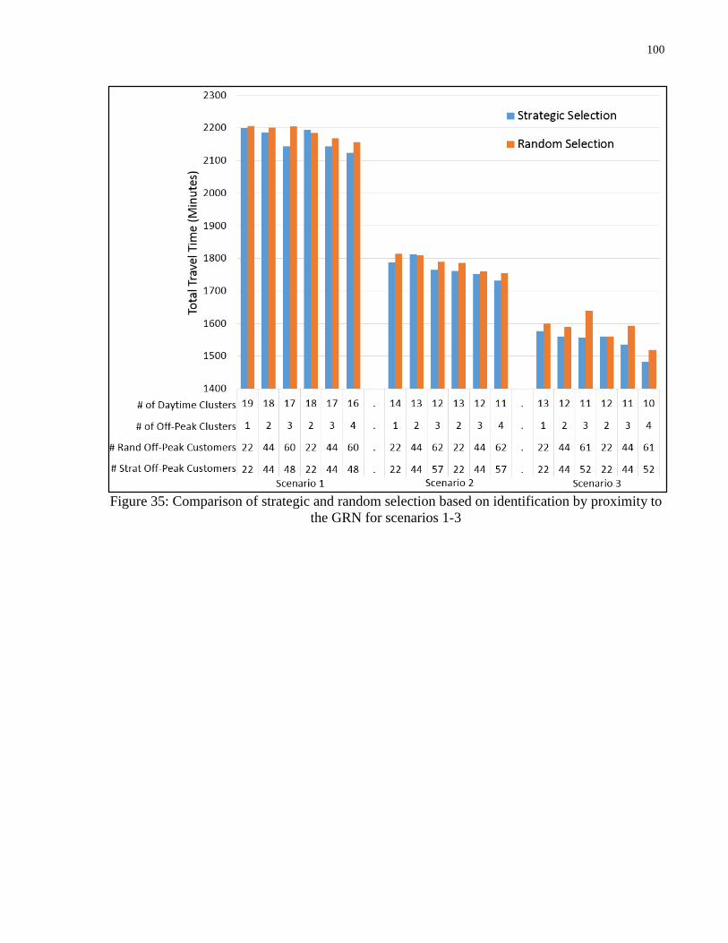
100
Figure 35: Comparison of strategic and random selection based on identification by proximity to
the GRN for scenarios 1-3

101
Figure 36: Comparison of strategic and random selection based on identification by proximity to
the GRN for scenarios 4-6
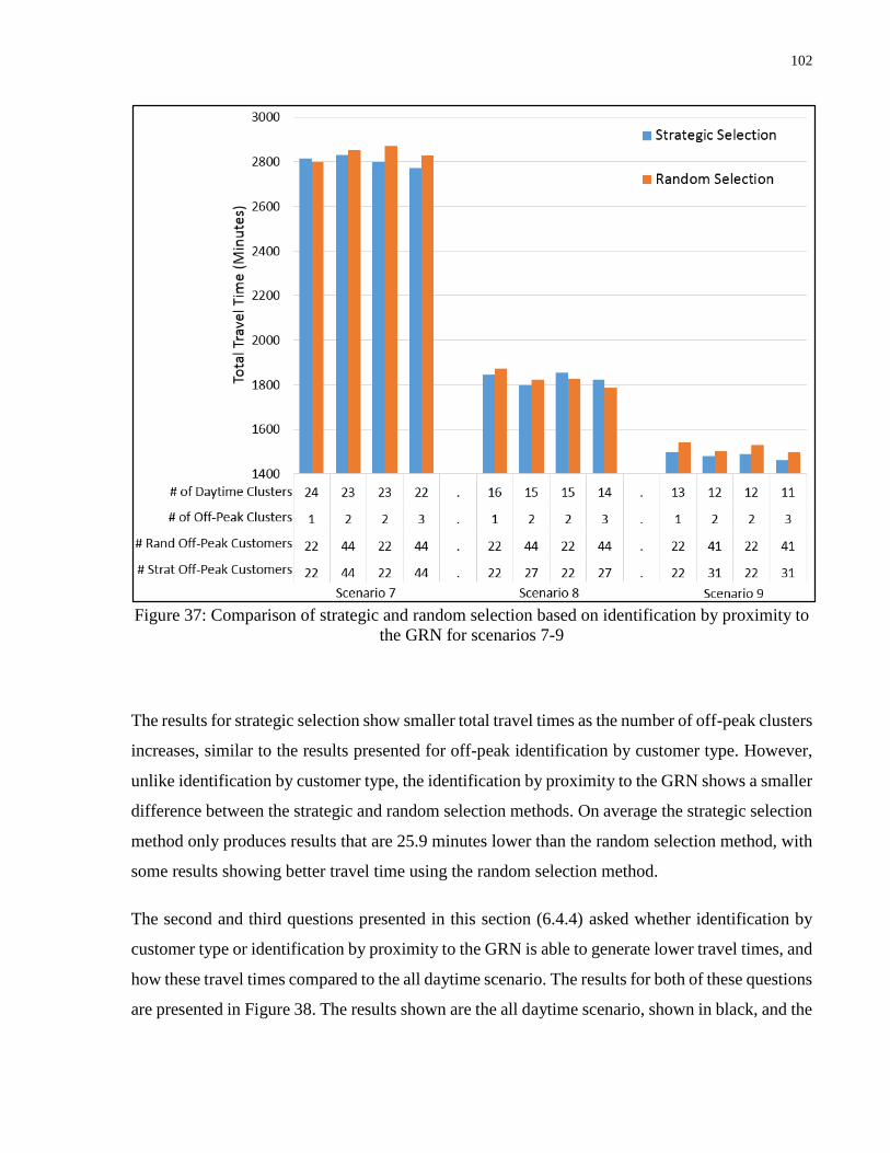
102
Figure 37: Comparison of strategic and random selection based on identification by proximity to
the GRN for scenarios 7-9
The results for strategic selection show smaller total travel times as the number of off-peak clusters
increases, similar to the results presented for off-peak identification by customer type. However,
unlike identification by customer type, the identification by proximity to the GRN shows a smaller
difference between the strategic and random selection methods. On average the strategic selection
method only produces results that are 25.9 minutes lower than the random selection method, with
some results showing better travel time using the random selection method.
The second and third questions presented in this section (6.4.4) asked whether identification by
customer type or identification by proximity to the GRN is able to generate lower travel times, and
how these travel times compared to the all daytime scenario. The results for both of these questions
are presented in Figure 38. The results shown are the all daytime scenario, shown in black, and the

103
four combinations of off-peak customer identification and selection. The numbers for these four
combinations are averaged from the total travel times presented in Figures 32-37.
Figure 38: Comparison of total travel times for all off-peak selection methods
Figure 38 shows improvement over the all daytime scenario for all strategic selection methods,
both using identification by customer type and proximity to the GRN, with the exception of
scenario 9 identification by customer type. For most scenarios, 7 out of 9, both the random and
strategic selection by proximity to the GRN generates lower average travel times compared to
identification by customer type, as well as larger maximum travel time decreases. This indicates
that there is some benefit to focusing off-peak delivery efforts on customers surrounding the GRN.
The summary of travel time decreases for each scenario from the all daytime scenario is shown in
Table 12. The numbers displayed are the average travel time percentage differences and maximum
travel time decreases for each customer selection and identification method. For this table, the
positive numbers represent travel time decreases from the all daytime scenario, while the negative
numbers represent travel time increases when compared to the all daytime scenario.
1400
1600
1800
2000
2200
2400
2600
2800
3000
Scenario1
Scenario2
Scenario3
Scenario4
Scenario5
Scenario6
Scenario7
Scenario8
Scenario9
Tota
l Tra
vel T
ime
(Min
ute
s)
All Daytime Strategic Selection by Customer Type
Random Selection by Customer Type Strategic Selection by Proximity to the GRN
Random Selection by Proximity to the GRN
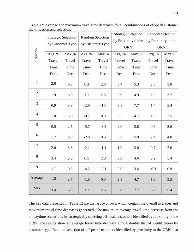
104
Table 12: Average and maximum travel time decreases for all combinations of off-peak customer
identification and selection.
Sce
nar
io
Strategic Selection
by Customer Type
Random Selection
by Customer Type
Strategic Selection
by Proximity to the
GRN
Random Selection
by Proximity to the
GRN
Avg. %
Travel
Time
Dec.
Max %
Travel
Time
Dec.
Avg. %
Travel
Time
Dec.
Max %
Travel
Time
Dec.
Avg. %
Travel
Time
Dec.
Max %
Travel
Time
Dec.
Avg. %
Travel
Time
Dec.
Max %
Travel
Time
Dec.
1 2.8 6.3 0.3 2.6 3.4 5.3 2.5 3.8
2 1.9 3.8 1.1 2.5 2.9 4.9 2.0 3.7
3 0.9 3.8 -2.9 -1.0 3.8 7.7 1.4 5.4
4 1.8 3.0 -0.7 0.9 3.5 4.7 1.6 2.5
5 0.5 2.5 -5.7 -3.8 2.0 2.8 0.6 2.6
6 1.7 3.9 -2.8 0.3 3.6 5.8 2.4 4.8
7 2.0 3.8 -2.1 -1.1 1.9 3.0 0.7 2.0
8 3.4 5.5 0.5 2.0 3.0 4.6 3.2 5.4
9 -1.9 0.3 -4.2 -2.1 2.0 3.4 -0.3 0.9
Average 1.5 3.7 -1.8 0.0 2.9 4.7 1.6 3.5
Max 3.4 6.3 1.1 2.6 3.8 7.7 3.2 5.4
The key data presented in Table 12 are the last two rows, which contain the overall averages and
maximum travel time decreases generated. The maximum average travel time decrease from the
all daytime scenario is by strategically selecting off-peak customers identified by proximity to the
GRN. The results show an average travel time decrease almost double that of identification by
customer type. Random selection of off-peak customers identified by proximity to the GRN also
105
produces better total travel times than strategic selection based on customer type. For random
selection based on customer type, the average total travel time is higher than the all daytime
scenario, indicating that there are no travel time benefits to be gained from using that method.
In terms of planning for a large sporting event like the Pan Am Games, these results demonstrate
the need for complete information concerning the GRN to be available to companies well in
advance of the Games. Customers situated in close proximity to the GRN are the most likely to be
impacted during the Games, and the data shows that focusing on these customers can bring the
greatest travel time benefits. There are also benefits to be had from parking search time which is
generally easier at night, but also would be more difficult during the Games due to parking
restrictions on the GRN.
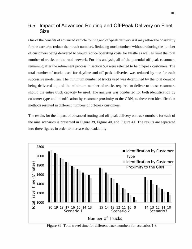
106
6.5 Impact of Advanced Routing and Off-Peak Delivery on Fleet Size
One of the benefits of advanced vehicle routing and off-peak delivery is it may allow the possibility
for the carrier to reduce their truck numbers. Reducing truck numbers without reducing the number
of customers being delivered to would reduce operating costs for Nestlé as well as limit the total
number of trucks on the road network. For this analysis, all of the potential off-peak customers
remaining after the refinement process in section 5.4 were selected to be off-peak customers. The
total number of trucks used for daytime and off-peak deliveries was reduced by one for each
successive model run. The minimum number of trucks used was determined by the total demand
being delivered to, and the minimum number of trucks required to deliver to those customers
should the entire truck capacity be used. The analysis was conducted for both identification by
customer type and identification by customer proximity to the GRN, as these two identification
methods resulted in different numbers of off-peak customers.
The results for the impact of advanced routing and off-peak delivery on truck numbers for each of
the nine scenarios is presented in Figure 39, Figure 40, and Figure 41. The results are separated
into three figures in order to increase the readability.
Figure 39: Total travel time for different truck numbers for scenarios 1-3
1000
1200
1400
1600
1800
2000
2200
20 19 18 17 16 15 14 13 15 14 13 12 11 10 9 14 13 12 11 10Tota
l Tra
vel T
ime
(Min
ute
s)
Scenario 1 Scenario 2 Scenario3
Identification by CustomerTypeIdentification by CustomerProximity to the GRN
Number of Trucks

107
Figure 40: Total travel time for different truck numbers for scenarios 4-6
Figure 41: Total travel time for different truck numbers for scenarios 7-9
1000
1200
1400
1600
1800
2000
2200
2400
18 17 16 15 14 13 12 11 19 18 17 16 15 14 13 12 16 15 14 13 12 11
Tota
l Tra
vel T
ime
(Min
ute
s)
Scenario 4 Scenario 5 Scenario 6
Identification by CustomerTypeIdentification by CustomerProximity to the GRN
Number of Trucks
1000
1200
1400
1600
1800
2000
2200
2400
2600
2800
3000
25 24 23 22 21 20 19 18 17 16 15 14 17 16 15 14 13 12 11 14 13 12 11 10
Tota
l Tra
vel T
ime
(Min
ute
s)
Scenario 7 Scenario 8 Scenario 9
Identification by CustomerTypeIdentification by CustomerProximity to the GRN
Number of Trucks

108
The results in Figure 39, Figure 40, and Figure 41 show consistent travel time decreases as a result
of reducing truck numbers. The percentage travel time decrease from the highest to the lowest
truck number, averaged over all nine scenarios, is 26.6% when potential off-peak customers are
identified by type and 28.4% when potential off-peak customers are identified by proximity to the
GRN. The average travel time decrease expected by reducing truck numbers by one is 4.8% and
5.2% for potential off-peak customers identified by customer type and proximity to the GRN
respectively.
The possibility for reducing truck numbers is more of a function of the advanced routing rather
than the off-peak delivery. Section 6.3 shows the benefits advanced routing can have over the call-
and-place delivery method without changing the number of trucks being used. The cluster-first
route-second method allows for higher utilization of each truck’s total capacity. It has been shown
that off-peak delivery can reduce the overall travel time required to make all deliveries.

109
Chapter 7
Conclusion
This thesis first examined the challenges introduced by large sporting events to urban good
movements and the best practices used by stakeholders during these events, and then analyzed the
possibility of using off-peak delivery to help mitigate some of these impacts, with a specific focus
on the travel time impacts. This concluding chapter will summarize the important points and
findings from qualitative and each of the quantitative analyses. It will conclude by briefly
discussing some limitations of the work presented and some recommendations for future research.
7.1 Best Practices for Goods Movement during Sporting Events
One of the primary research objectives for this project was to examine the impact of large sporting
events and to determine best practices for urban freight movement during these events. A series of
interviews was conducted with stakeholders in the London freight community who had first-hand
experience preparing and participating in freight logistics during the 2012 London Olympics. The
questions posed to them were concerned with what did and did not go well for their respective
organizations during the Olympics, what they might do differently given a second chance, and
finally whether they incorporated some form of off-peak delivery during the Olympics.
The two overarching themes present in the interview responses were the need to introduce freight
early on in the planning process, and to have one consistent and reliable source of information for
freight stakeholders. Introducing freight early helps ensure that the issues of major concern to
freight operators and stakeholders are factored into the decision making process. Maintaining one
consistent and reliable source of information allows individual companies and their customers to
plan for the Games accordingly with the most up to date knowledge of road conditions and
restrictions.
110
7.2 Impact of the Pan Am Games on Normal Operations
The first research question was concerned with the impact that the Pan Am Games would have on
Nestlé’s normal operations should Nestlé not make any changes in preparation of the Games. The
results show a travel time difference of 6.4% between the Games and BAU conditions. This 6.4%
represents an average travel time increase of 171 minutes per week. This increase in travel times
is only one of the expected impacts from the Games. Parking and delivery restrictions in and
around the GRN and event venues are also expected to cause further delays and longer tour times
for Nestlé’s delivery vehicles.
7.3 Impact of Advanced Routing on Travel Times
The travel time benefits of advanced route planning over call-and-place delivery methods of
routing were shown by comparing delivery log travel times for Nestlé deliveries against a capacity
constrained k-means clustering algorithm. The results showed an average potential travel time
savings of 26% when routing on a weekly basis. The reason behind the large decreases in travel
time is that there is a possibility of generating much more compact and localized clusters. This
would reduce the in-between customer travel time, and in some cases may also allow for multiple
deliveries to be made from the same parking location.
7.4 Potential of Off-Peak Delivery in Minimizing Travel Times
The results for the off-peak delivery analysis show that travel time improvements are possible by
incorporating off-peak delivery into normal operations. Four methods for generating off-peak
routes were used: strategic selection using off-peak customer identification by type, strategic
selection using off-peak customer identification by proximity to the GRN, random selection using
off-peak customer identification by type, and finally random selection using off-peak customer
identification by proximity to the GRN. The results showed that the greatest travel time benefits
could be made by incorporating strategic selection, and by focusing on customers situated in close
proximity to the GRN, resulting in an average of 2.9% below the all daytime scenario. Travel time
decreases were also generated for strategic selection by customer type and random selection by

111
proximity to the GRN, at 1.5% and 1.6% respectively. In terms of policy, these results indicate
that efforts should be placed on getting customers near the GRN to participate in off-peak delivery
programs.
7.5 Potential of Advanced Routing and Off-Peak Delivery in Reducing Fleet Size
A significant benefit of advanced routing over the call-and-place methods is that, in addition to
generating more compact and localized clusters, it introduces the possibility of reducing the total
number of trucks required to make the deliveries. Routes can be configured that utilize more of a
trucks capacity, allowing carriers to reduce the total number of trucks required. The analysis
conducted shows fairly consistent total travel time decreases of 4.8% and 5.3% per truck removed
depending on whether the off-peak customers were identified based on customer type or by
proximity to the GRN, respectively.
7.6 Limitations and Recommendations for Future Research
There are several limitations to this project that need to be mentioned. Some of these limitations
were necessary due to the quality and quantity of the data available, while other were practical
limitations to simplify the models. Assumptions were made concerning the customer’s likelihood
of accepting off-peak delivery. The assumption was made based upon what type of customer was
being delivered to, and whether that customer routinely operates in some capacity during the off-
peak hours. Ideally a full survey of customers would be required to generate the list of potential
off-peak customers. This would give Nestlé the greatest likelihood of maximizing their travel time
savings. However, for this project a survey of customers was not practical, and therefore the
assumptions had to be made.
An assumption was made concerning the size of the delivery truck used in all of the deliveries.
Nestlé uses three different truck sizes to make deliveries, but only one size was chosen to simplify
the models. Delivery logs did not contain information about what size of truck was used to make
the deliveries.

112
The travel time tables provided were average travel time values between TTS zones. There is a
loss of accuracy in vehicle routing using actual customer locations combined with zonal travel
times. This is unavoidable as actual travel times between specific customer locations would be
challenging to generate. Another limitation is the lack of intrazonal travel times provided by IBI.
An estimate had to be made for travel time between customers in the same zone. This estimate is
used whether the customers are right next to one another or on the opposite side of the zone.
The decision as to whether to include a customer in off-peak delivery was based solely on the total
travel times. In reality there would be more to consider when making those decisions. Parking time
and delivery time are two key components in determining the total time a truck is out making
deliveries. Some research has shown that there can be significant improvements in both the parking
and delivery time when deliveries are made during the off-peak hours. It is possible that a carrier
like Nestlé would be willing to make some sacrifices in travel time in order to make greater benefits
in overall tour times. Since parking and delivery time were not estimated, these two factors were
ignored.
There are several policy implications for the carriers and their drivers which may impact the
possibility of an off-peak delivery program being implemented. The switch from daytime to
nighttime deliveries would also require truck driver’s approval, as it is possible that many of them
would not be willing to deliver at night. Extra costs may also be required not only for driver pay,
but also for potentially higher insurance costs and the cost for adding low noise technology to
existing vehicles. A larger study would have to be conducted including the cost analysis in addition
to the tour time estimates before a final decision could be made concerning the total costs and
benefits of an off-peak delivery program.
There are two key aspects of off-peak delivery for which there are still gaps in the current literature.
One of the benefits of off-peak delivery is the reduction in parking search time. Delivering during
off-peak hours would not only benefit the carriers in reduced delivery times, but the daytime traffic
as well which would benefit from reduced truck numbers during the day. Knowing the benefits for
reduced parking search time would allow for a more complete picture of off-peak delivery, and
would allow carriers to make more informed decisions concerning their use of off-peak delivery.
The second gap in the current literature is related to the environmental impact of off-peak delivery.
More specifically, the differences in truck emissions as a result of changes in average speed and

113
dwell time during the off-peak hours. It is possible that the positive possible externalities
associated with off-peak delivery would help to drive policy changes that would allow for reduced
restrictions for off-peak delivery implementation.

114
References
Augerat, P., Belenguer, J., Benavent, E., Corberan, A., & Naddef, D. (1998). Separating
Capacity Constraints in the CVRP using tabu search. European Journal of Operational
Research, 106(2-3), 546-557.
Bock, H. (2008). Origins and Extensions of the k-Means Algorithm in Cluster Analysis.
Electronic Journal for the History of Probability and Statistics, 4(2) (2008).
Bodin, L., & Golden, B. (1981). Classification in Vehicle Routing and Scheduling. Networks,
11(2), 97-108.
Bradley, P., & Fayyad, U. (1998). Refining Initial Points for K-Means Clustering. ICML, 98, 91-
99.
Bradley, P., Bennett, K., & Demiriz, A. (2000). Constrained k-means clustering. Redmond:
Microsoft Research, MSR-TR-2000-65, 2000.
Brom, M., Holguin-Veras, J., & Hodge, S. (2014). Off-Hour Deliveries in Manhatten, New York
City: Experience of Pilot Test Participants. Transportation Research Record: Journal of
the Transportation Research Board, 2238, 77-85.
Browne, M., Allen, J., Wainwright, J., Palmer, A., & Williams, I. (2014). London 2012:
Changing Delivery Patterns in Response to the Impact of the Games on Traffic Flows.
International Journal of Urban Sciences, 18(2), 244-261.
Campbell, J. (1995). Peak Period Large Truck Restrictions and a Shift to Off-Peak Operations:
Impact on Truck Emissions and Performance. Journal of Business Logistics, 16(2), 227-
247.
Chiffi, C. (2014, 12). Silent Inner-City Overnight Deliveries in Barcelona (Spain). Retrieved
from Eltis: http://www.eltis.org/discover/case-studies/silent-inner-city-overnight-
deliveries-barcelona-spain

115
Churchill, J. (1970). Operation moondrop: An Experiment in Out of Hours Goods Delivery. In
The Urban Movements of Goods (pp. 135-140). Paris: OCED.
Davidson, I., & Ravi, S. (2005). Agglomerative Hierarchical Clustering wth Constraints:
Theoretical and Empirical Results. In Knowledge Discovery in Databases: Lecture Notes
in Compter Science (Vol. 3721, pp. 59-70). New York.
DMG (2011). Transportation Tomorrow Survey. Retrieved from Data Management Group:
University of Toronto: http://dmg.utoronto.ca/#
Fisher, M., & Jaikumar, R. (1981). A Generalized Assignment Heuristic for Vehicle Routing.
Networks, 11, 109-124.
Freight Transport Association. (2011). Managing Deliveries and Services during the Olympic
Games. London, England: Freight Transport Association.
Freight Transport Association. (2012). Logistics Legacy - Celebrating Logistics Achievement and
Innovation during Summer 2012. London, England: Freight Transport Association.
Geetha, S., Poonthalir, G., & Vanathi, P. (2009). Improved K-Means Algorithm for Capacitated
Clustering Problem. INFOCOMP Journal of Computer Science, 8(4), 52-59.
Hartigan, J., & Wong, M. (1979). Algorithm AS 136: A K-Means Clustering Algorithm. Journal
of the Royal Statistical Society. Series C (Applied Statistics), 28(1), 100-108.
Hirst, M. (2012, July 25). London 2012 Olympic Route Network Q&A. Retrieved from bbc.com:
http://www.bbc.com/news/uk-16277688
Holguin-Veras, J. (2014, 02). The Lessons from the Off-Hour Delivery Project in New York City.
Freight Day iii Symposium 2014. University of Toronto. Toronto, Canada. Retrieved
from UTTRI:
http://www.civil.engineering.utoronto.ca/Assets/Civil+Engineering+Digital+Assets/aUT
TRI/2.2+Jose+Holguin-Veras+Off-Hour+Deliveries+in+NYC+Lessons+Learned.pdf
116
Holguin-Veras, J., Ozbay, K., Kornhauser, A., Brom, M., Iyer, A., Yushimito, W., Silas, M.
(2014b). Overall Impacts of Off-Hour Delivery Programs in New York City Metropolitan
Area. Procedia - Social and Behavioral Sciences, 125, 36-48.
Holguin-Veras, J., Perez, N., Cruz, B., & Polimeni, J. (2007c). Effectiveness of Financial
Incentives for Off-Peak Deliveries to Restaurants in Manhattan, New York.
Transportation Research Record: Journal of the Transportation Research Board Volume
1966, 51-59.
Holguin-Veras, J., Polimeni, J., Cruz, B., Xu, N., Nordstrom, J., & Haddock, J. (2005). Off-Peak
Deliveries: Challanges and Stakeholders Perceptions. Transportation Research Record:
Journal of the Transportation Research Board 1906, 42-48.
Holguin-Veras, J., Silas, M., Polimeni, J., & Cruz, B. (2007). An Investigation on the
Effectiveness of Joint Receiver Carrier Policies to Increase Truck Traffic in the Off-Peak
Hours - Part I. Networks and Spatial Economics, 7(3), 277-295.
Holguin-Veras, J., Silas, M., Polimeni, J., & Cruz, B. (2007b). An Investigation on the
Effectiveness of Joint Receiver-Carrier Policies to Increase Truck Traffic in the Off-Peak
Hours-Part ii: The Behavior of Carriers. Networks and Spatial Economics, 8(4), 327-354.
Holguin-Veras, J., Wang, C., Browne, M., Hodge, S., & Wojtowicz, J. (2014a). The New York
City Off-Hour Delivery Project: Lessons for City Logistics. Procedia - Social and
Behavioral Sciences, 125, 36-48.
Holguin-Veras, J., Wang, X., Hodge, S., Campbell, S., Sanchez-Diaz, I., Marquis, R.,
Wojtowicz, J. (2013). Fostering the Use of Unassisted Off-Hour Deliveries: Operational
and Low Noise Truck Technologies. Transportation Research Record, Journal of the
Transportation Research Board 2379, 57-63
Jain, A. (2010). Data clustering: 50 years beyond K-means. Pattern Recognition Letters, 31(8),
651-666.
Kallehauge, B., Larsen , J., Madsen, O., & Solomon, M. (2005). Vehicle Routing Problem with
Time Windows. Springer US.
117
Kim, K. Y. (2007). Using a K-means Clustering Algorithm to Examine Patterns of Pedestrian
Involved Crashes in Honolulu, Hawaii. Journal of Advanced Transportation, 41(1), 69-
89.
Koskosidis, Y., & Powell, W. (1992). Clustering Algorithms for Consolidation of Custom Orders
into Vehicle Shipments. Transportation Research Part B: Methodological, 26(5), 365-
379.
Lam, M., & Mittenthal, J. (2013). Capacitated Hierarchical Clustering Heuristic for Multi-Depot
Location Routing Problems. International Journal of Logistics Research and
Applications: A Leading Journal of Supply Chain Management, 16(5), 433-444.
Laporte, G. (1992). The Vehicle Routing Problem: An Overview of Exact and Approximate
Algorithms. European Journal of Operational Research, 59(3), 345-358.
Laporte, G., Desrochers, M., & Norbert, Y. (2006). Two Exact Algorithms for the Distance-
Constrained Vehicle Routing Problem. Networks, 14(1), 161-172.
Lloyd, S. (1982). Least Squares Quantization in PCM. Transactions on Information Theory,
28(2), 129-137.
Manning, C., Raghavan, P., & Schutze, H. (2008). Hierarchical clustering. In Introduction to
Information Retrieval (pp. 377-378). Cambridge: Cambridge University Press.
Martin, W., & McGuckin, N. (1998). NCHRP Report 365: Travel Estimation Techniques for
Urban Planning. Transportation Research Board: National Cooperative Highway
Research Program.
Maulik, U., & Bandyopadhyay, S. (2000). Genetic Algorithm-based Clustering Technique.
Pattern Recognition, 33, 1455-1465.
Metrolinx. (2011). GTHA Urban Freight Study: Final Draft. Toronto: Metrolinx.
Mitchell, M. (1998). An Introduction to Genetic Algorithms. Boston: MIT Press.

118
Moore, O. (2015, 01). Tory Begins Crackdown on Illegal Rush Hour Parking. Retrieved from
The Globe and Mail: http://www.theglobeandmail.com/news/toronto/toronto-begins-
crackdown-on-illegal-rush-hour-parking/article22288949/
O'Laughin, R., Rinnan, M., & Thomas, D. (2008). Chicago Downtown Freight Study.
Transportation Research Board 87th Annual Meeting. Washington. DC. 2008
Ministry of Transportation of Ontario (2014). Keeping Your Business Moving - Creating a
Games Travel Plan. Toronto: MTO. Retrieved from
https://dr6j45jk9xcmk.cloudfront.net/documents/3840/full-guide-en.pdf
Ministry of Transportation of Ontario (2014a). Strategic Framework for Transportation -
Executive Summary. Toronto: IBI Group. Retrieved from
http://www.mto.gov.on.ca/english/pubs/pan-am-Games/strategic-framework-for-
transportation-executive-summary.pdf
Ministry of Transportation of Ontario (2014b). Volume one - Strategic Framework for
Transportation. Toronto: IBI Group. Retrieved from
http://www.ontario.ca/document/pan-amparapan-am-games-strategic-framework-
transportation-volume-1
Ministry of Transportation of Ontario (2014c). Off-Peak Deliveries (OPD) Pilot and Toolkit.
Toronto: MTO. Retrieved from
Ministry of Transportation of Ontario (2015). Route Planner. Retrieved from 2015 Toronto Pan
Am Games: https://2015gamestripplanner.ca/
O'Sullivan, F. (2012, 03 14). The PR Distaster of London's Olympic Traffic Lanes. Retrieved
from CityLab: http://www.citylab.com/politics/2012/03/pr-disaster-londons-olympic-
lanes/1486/
Pamula, R., Deka, J., & Nandi, S. (2011). An Outlier Detection Method based on Clustering.
Emerging Applications of Information Technology, (pp. 253-256). Kolkata.
Renaud, J., Boctor, F., & Laporte, G. (1996). An Improved Petal Heuristic for the Vehicle
Routing Problem. Journal of the Operational Research Society, 47, 329-336.

119
Roorda, M. J., Hain, M., Amirjamshidi, G., Cavalcante, R., Abdulhai, B., & Woudsma, C.
(2010). Exclusive Truck Facilities in Toronto, Ontario, Canada. Transportation Research
Record: Journal of the Transportation Research Board, 2168, 114-128.
Roorda, M., Miller, E. J., & Kruchten, N. (2006). Incoporating Within-Household Iterations into
Mode Choice Model with Genetic Algorithm for Parameter Estimation. Transportation
Research Record: Journal of the Transportation Research Board, 1985, 171-179.
Shoup, D. (2005). The High Cost of Free Parking. Chicago: Planners Press.
The Olympic Route Network. (2012). Retrieved from Bishops Gate:
http://www.bishopsgate.co.uk/wp/wp-content/uploads/2012/04/ORN_Overview.jpg
City of Toronto (2014). About the Pan American Games. Retrieved from Toronto 2015:
http://www.toronto2015.org/about-us/pan-am-games
Transport for London. (2013a). The Olympic and Paralympic Games - Transportation Legacy
0ne Year on. London, England: TFL. Retrieved from http://www.tfl.gov.uk/info-
for/media/press-releases/2013/july/the-london-2012-Games-transport-legacy-one-year-on
Transport for London. (2013b). Olympic Legacy Monitoring: Adaptations to Deliveries by
Businesses and Freight Operators during the Games. London, England: Transport for
London. Retrieved from http://www.tfl.gov.uk/cdn/static/cms/documents/olympic-
legacy-freight-report.pdf
U.S Department of Transportation Federal Highways Administration. (2013). HOV-to-HOT
Lanes Workshop. Retrieved from
http://ops.fhwa.dot.gov/freewaymgmt/publications/documents/nrpc0610/workshop_mater
ials/hov_to_hot/tabletop_poster.htm
Wang, C., Zhou, Y., Goevaers, R., Holguin-Veras, J., Wojtowicz, J., & Campbell, S. (2013).
Feasibility of Installing Noise Reduction Technologies on Commercial Vehicles to
Support Off-Hour Deliveries No. 25733. New York: Rensselaer Polytechnic Institute.
Wenneman, A., Habib, K., & Roorda, M. A Disaggregate Analysis of the Relationship Between
Commercial Vehicle Parking Citations, Parking Supply, and Parking Demand: Critical
120
Understandings and Policy Implications. Transportation Research Record: Journal of the
Transportation Research Board. (Forthcoming)
Wikipedia. (2015, May 11). Pan American Games. Retrieved from Wikipedia:
http://en.wikipedia.org/wiki/Pan_American_Games
Winkenbach, M., Kleindorfer, P., Lemarie, B., Leveque, C., Roset, A., & Spinler, S. (2012). A
Mixed Integer Linear Programming Model for Solving Large-Scale Integrated Location-
Routing Problems for Urban Logistics Applications at Groupe la Poste.Working Paper.
Retrieved from
http://idei.fr/sites/default/files/medias/doc/conf/pos/papers_2012/winkenbach.pdf.
Yannis, G., Golias, J., & Constantinos, A. (2007). Effects of Urban Delivery Restrictions on
Traffic Movements. Transportation Planning and Technology, 29(4), 295-311.
Zalik, K. (2008). An Efficient k-Means Clustering Algorithm. Pattern Recognition Letters,
29(9), 1385-1391.

121
Appendix A
Table A1: Travel time results for random selection by customer type
Scenario
Number of
Off-Peak
Clusters
Number
of Peak
Clusters
Number of
Off-Peak
Customers
Number of
Peak
Customers
% of Off-
Peak
Customers
Total Travel
Time
(minutes)
2 1
14 22 115 16.1 1836
2 2 13 28 109 20.4 1797
2 2 13 22 115 16.1 1800
2 3 12 28 109 20.4 1777
3 1
13 22 139 13.7 1695
3 2 12 38 123 23.6 1656
3 2 12 22 139 13.7 1639
3 3 11 38 123 23.6 1623
4 1
17 22 170 11.5 2064
4 2 16 44 148 22.9 2081
4 2 16 22 170 11.5 2016
4 3 15 44 148 22.9 2009
5 1
18 19 192 9.0 2381
5 2 17 34 177 16.1 2301
5 3 16 56 155 26.5 2373
5 2 17 19 192 9.0 2295
5 3 16 34 177 16.1 2305
5 4 15 56 155 26.5 2378
6 1
15 11 161 6.4 1862
6 2 14 32 140 18.6 1913
6 3 13 52 120 30.2 2027
6 4 12 62 110 36.0 1952
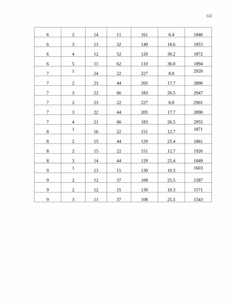
122
6 2 14 11 161 6.4 1846
6 3 13 32 140 18.6 1853
6 4 12 52 120 30.2 1872
6 5 11 62 110 36.0 1894
7 1
24 22 227 8.8 2920
7 2 23 44 205 17.7 2890
7 3 22 66 183 26.5 2947
7 2 23 22 227 8.8 2901
7 3 22 44 205 17.7 2890
7 4 21 66 183 26.5 2955
8 1
16 22 151 12.7 1871
8 2 15 44 129 25.4 1861
8 2 15 22 151 12.7 1926
8 3 14 44 129 25.4 1849
9 1
13 15 130 10.3 1603
9 2 12 37 108 25.5 1587
9 2 12 15 130 10.3 1571
9 3 11 37 108 25.5 1543

123
Table A2: Travel time results for random selection by proximity to the GRN
Scenario
Number of
Off-Peak
Clusters
Number
of Peak
Clusters
Number of
Off-Peak
Customers
Number of
Peak
Customers
% of Off-
Peak
Customers
Total Travel
Time
(minutes)
2 1
14 22 115 16.1 1814
2 2 13 44 93 32.1 1809
2 3 12 62 75 45.3 1790
2 2 13 22 115 16.1 1786
2 3 12 44 93 32.1 1759
2 4 11 62 75 45.3 1755
3 1
13 22 139 13.7 1600
3 2 12 44 117 27.3 1590
3 3 11 61 100 37.9 1640
3 2 12 22 139 13.7 1560
3 3 11 44 117 27.3 1594
3 4 10 61 100 37.9 1520
4 1
17 22 170 11.5 2003
4 2 16 44 148 22.9 1998
4 2 16 22 170 11.5 2005
4 3 15 44 148 22.9 1978
5 1
18 22 189 10.4 2188
5 2 17 44 167 20.9 2210
5 3 16 55 156 26.1 2236
5 2 17 22 189 10.4 2187
5 3 16 44 167 20.9 2155

124
5 4 15 55 156 26.1 2214
6 1
15 22 150 12.8 1835
6 2 14 44 128 25.6 1812
6 2 14 22 150 12.8 1819
6 3 13 44 128 25.6 1762
7 1
24 22 227 8.8 2800
7 2 23 44 205 17.7 2853
7 2 23 22 227 8.8 2869
7 3 22 44 205 17.7 2826
8 1
16 22 151 12.7 1871
8 2 15 44 129 25.4 1822
8 2 15 22 151 12.7 1825
8 3 14 44 129 25.4 1784
9 1
13 22 123 15.2 1541
9 2 12 41 104 28.3 1501
9 2 12 22 123 15.2 1528
9 3 11 41 104 28.3 1498

125
Table A3: Travel time results for strategic selection by customer type
Scenario
Number of
Off-Peak
Clusters
Number
of Peak
Clusters
Number of
Off-Peak
Customers
Number of
Peak
Customers
% of Off-
Peak
Customers
Total Travel
Time
(minutes)
2 1 14 22 115 16.1 1822
2 2 13 25 112 18.2 1790
2 2 13 22 115 16.1 1784
2 3 12 25 112 18.2 1752
3 1 13 22 139 13.7 1631
3 2 12 28 133 17.4 1600
3 2 12 22 139 13.7 1593
3 3 11 28 133 17.4 1546
4 1 17 22 170 11.5 2014
4 2 16 28 164 14.6 2012
4 2 16 22 170 11.5 1976
4 3 15 28 164 14.6 1968
5 1 18 20 191 9.5 2236
5 2 17 39 172 18.5 2206
5 3 16 45 166 21.3 2222
5 2 17 20 191 9.5 2215
5 3 16 39 172 18.5 2174
5 4 15 45 166 21.3 2157
6 1 15 16 156 9.3 1792
6 2 14 36 136 20.9 1832

126
6 3 13 48 124 27.9 1877
6 4 12 54 118 31.4 1849
6 2 14 16 156 9.3 1827
6 3 13 36 136 20.9 1806
6 4 12 48 124 27.9 1793
6 5 11 54 118 31.4 1779
7 1 24 22 227 8.8 2829
7 2 23 44 205 17.7 2818
7 3 22 52 197 20.9 2750
7 2 24 22 227 8.8 2808
7 3 22 44 205 17.7 2799
7 4 21 52 197 20.9 2795
8 1 16 22 151 12.7 1861
8 2 15 34 139 19.7 1803
8 2 15 22 151 12.7 1843
8 3 14 34 139 19.7 1783
9 1 13 22 123 15.2 1584
9 2 12 35 110 24.1 1541
9 2 12 22 123 15.2 1530
9 3 11 35 110 24.1 1507
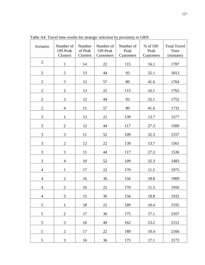
127
Table A4: Travel time results for strategic selection by proximity to GRN
Scenario
Number of
Off-Peak
Clusters
Number
of Peak
Clusters
Number of
Off-Peak
Customers
Number of
Peak
Customers
% of Off-
Peak
Customers
Total Travel
Time
(minutes)
2 1 14 22 115 16.1 1787
2 2 13 44 93 32.1 1813
2 3 12 57 80 41.6 1764
2 2 13 22 115 16.1 1762
2 3 12 44 93 32.1 1752
2 4 11 57 80 41.6 1732
3 1 13 22 139 13.7 1577
3 2 12 44 117 27.3 1560
3 3 11 52 109 32.3 1557
3 2 12 22 139 13.7 1561
3 3 11 44 117 27.3 1536
3 4 10 52 109 32.3 1483
4 1 17 22 170 11.5 1975
4 2 16 36 156 18.8 1969
4 2 16 22 170 11.5 1950
4 3 15 36 156 18.8 1932
5 1 18 22 189 10.4 2195
5 2 17 36 175 17.1 2167
5 3 16 49 162 23.2 2151
5 2 17 22 189 10.4 2166
5 3 16 36 175 17.1 2173

128
5 4 15 49 162 23.2 2161
6 1 15 22 150 12.8 1804
6 2 14 39 133 22.7 1797
6 2 14 22 150 12.8 1795
6 3 13 39 133 22.7 1743
7 1 24 22 227 8.8 2815
7 2 23 44 205 17.7 2830
7 2 23 22 227 8.8 2799
7 3 22 44 205 17.7 2773
8 1 16 22 151 12.7 1843
8 2 15 27 146 15.6 1799
8 2 15 22 151 12.7 1855
8 3 14 27 146 15.6 1824
9 1 13 22 123 15.2 1498
9 2 12 31 114 21.4 1478
9 2 12 22 123 15.2 1490
9 3 11 31 114 21.4 1460