The Impact of Layer Perturbation Potential Energy on the East AsianSummer Monsoon

LIDOU HUYAN,a,b JIANPING LI,c,d SEN ZHAO,e,f CHENG SUN,c DI DONG,a,b TING LIU,g AND YUFEI ZHAOh

a State Key Laboratory of Numerical Modeling for Atmospheric Sciences and Geophysical Fluid Dynamics,

Institute of Atmospheric Physics, Chinese Academy of Sciences, Beijing, ChinabUniversity of Chinese Academy of Sciences, Beijing, China

c State Key Laboratory of Earth Surface Processes and Resource Ecology, and College of Global

Change and Earth System Science, Beijing Normal University, Beijing, ChinadLaboratory for Regional Oceanography and Numerical Modeling, Qingdao National

Laboratory for Marine Science and Technology, Qingdao, Chinae School of Ocean and Earth Sciences and Technology, University of Hawai‘i at M�anoa, Honolulu, HawaiifKey Laboratory of Meteorological Disaster of Ministry of Education, and College of Atmospheric Science,

Nanjing University of Information Science and Technology, Nanjing, Chinag State Key Laboratory of Satellite Ocean Environment Dynamics, Second Institute of Oceanography, Hangzhou, China

hNational Meteorological Information Center, Beijing, China

(Manuscript received 9 October 2016, in final form 21 April 2017)

ABSTRACT

This paper analyzes the relationship between the 1000–850-hPa layer perturbation potential energy (LPPE)

as the difference in local potential energy between the actual state and the reference state and the East Asian

summer monsoon (EASM) using reanalysis and observational datasets. The EASM is closely related to the

first-order moment term of LPPE (LPPE1) from the preceding March to the boreal summer over three key

regions: the eastern Indian Ocean, the subtropical central Pacific, and midlatitude East Asia. The LPPE1

pattern (2, 1, 1), with negative values over the eastern Indian Ocean, positive values over the subtropical

central Pacific, and positive values over East Asia, corresponds to negative LPPE1 anomalies over the south

of the EASM region but positive LPPE1 anomalies over the north of the EASM region, which lead to an

anomalous downward branch over the southern region but an upward branch over the northern region. The

anomalous vertical motion affects the local meridional circulation over EastAsia that leads to a southwesterly

wind anomaly over East Asia (south of 308N) at 850 hPa and anomalous downward motion over 1008–1208E(along 258–358N), resulting in a stronger EASM, more kinetic energy over the EASM region, and less boreal

summer rainfall in the middle and lower reaches of the Yangtze River valley (248–368N, 908–1258E). TheseLPPE1 anomalies in the eastern Indian Ocean and subtropical central Pacific appear to be connected to

changes in local sea surface temperature through the release of latent heat.

1. Introduction

The climate of China is greatly affected by the East

Asian monsoon (Tao and Chen 1987). In particular, the

flood season, large-scale distribution of rainfall patterns,

rain belt movement, and extreme precipitation over

East Asia are associated with the East Asian summer

monsoon (EASM). Furthermore, drought and flood

events related to the EASMoften cause heavy economic

losses and casualties. Understanding the formation and

variation of the EASM will assist our understanding of

the effects of climate change, revealing patterns of

seasonal precipitation variability, and generating new

theories and methods for climate prediction. Therefore,

the EASM variability and its related climate anomalies

have received considerable attention (Li et al. 2011a,b,

2013).

Numerous studies have investigated the EASM and

have focused on, for example, the characteristics and

variability of the EASM (Li et al. 2004; Qian 2005; He

et al. 2006), interaction between the EASM and El

Niño–Southern Oscillation (ENSO; Lau and Nath 2000;

Wang et al. 2008b), the simulation and forecasting of the

East Asian monsoon (Wang et al. 2004), the impact on

the formation of ENSO (Li and Mu 1998), the sub-

tropical East Asian monsoon (He et al. 2004; Zhu et al.Corresponding author: Prof. Jianping Li, ljp@bnu.edu.cn

1 SEPTEMBER 2017 HUYAN ET AL . 7087

DOI: 10.1175/JCLI-D-16-0729.1

� 2017 American Meteorological Society. For information regarding reuse of this content and general copyright information, consult the AMS CopyrightPolicy (www.ametsoc.org/PUBSReuseLicenses).

2011), the impact of underlying processes on the EASM

(Liang andWu 2003; Zhang andLi 2004; Zuo andZhang

2016), the decadal variability of the EASM (Yang et al.

2005), and the kinetic energy (KE) of the Asian mon-

soon system (Guan 2000). Although there has been

much work and significant achievements in the field of

EASM research, our current forecast skill with respect

to the EASM is still not high and does not meet the

needs of production and life (e.g., Kang et al. 2002;

Wang et al. 2005; Song andZhou 2014). This implies that

our understanding of the dynamics and physical pro-

cesses associated with the EASM and its climatic im-

pacts needs to be improved, and that further exploration

in this field will be of both great theoretical significance

and practical value.

The ongoing evolution of the atmospheric circulation

is driven by the changing nature of the atmospheric

energy balance, and the variability of the EASM is re-

lated to the changes in the KE of the EASM circulation

(e.g., vanMieghem 1973; Li et al. 2016). Previous studies

have shown that the EASM is connected to the un-

derlying external forcing, such as sea surface tempera-

ture (SST) and snow cover (Guo and Wang 1986; Wu

et al. 2004, 2005; Zhang and Li 2004; Nan and Li 2005; Li

et al. 2011a,b; Zheng et al. 2014). However, the theory of

atmospheric energetics confirms that external diabatic

heating cannot be directly converted into KE, which

indicates that the variations of the underlying external

forcing are not the direct sources of the KE (e.g.,

Margules 1903; Lorenz 1955). Therefore, it is necessary

to explore the sources of KE within the EASM system.

In addition, there have been few studies of the vari-

ability of the EASM from the point of view of regional

energetics. Research from this new perspective is hoped

to bring a better understanding of the variability of the

EASM and its link to the external forcing.

The framework of modern atmospheric energetics is

based on Lorenz’s study of available potential energy

(APE; Lorenz 1955). Further development of the the-

ory of APE has aided our understanding of the effi-

ciency of energy conversion between APE and KE in

terms of the global mean (Johnson 1970; Bullock and

Johnson 1971; Gu 1990; Gao and Li 2007). However,

the application of APE is restricted because the con-

cept of APE is based on globally averaged variables,

which imposes limitations on the regional energy con-

version; consequently, modifications are required when

applying APE in the local region. Li and Gao (2006)

introduced the concept of perturbation potential en-

ergy (PPE), which indicates the maximum amount of

total potential energy that could be converted into KE

at the local scale. Locally, the first-order moment term

of PPE (PPE1) is an order of magnitude larger than the

second-order moment term of PPE (PPE2; Li and Gao

2006; Li et al. 2016).

According to Gao and Li (2012, 2013), PPE is closely

related to the atmospheric circulation variability, and

they also analyzed the characteristics of the surface

perturbation potential energy. To investigate energy

transformation features at different levels in the light of

the baroclinic of atmosphere, Wang et al. (2012) in-

troduced the concept of layer perturbation potential

energy (LPPE) and also applied the theory to explore

the variability of the South China Sea summer monsoon

(Wang et al. 2013). The atmospheric PPE has been used

to study variations in tropical Pacific atmospheric

available energetics during an ENSO cycle (Dong et al.

2017). These previous results indicate that PPE is a key

link between the local diabatic heating and the vari-

ability of KE for circulation. Therefore, the PPE theory

can provide a new perspective for studying the ener-

getics of the regional circulation of the EASM and a

theoretical foundation from which to examine the

sources and variability of the KE of the EASM (Li et al.

2016). We should also consider that there are compli-

cated external forcings that exert effect on the vari-

ability of EASM, such as ENSO, the tropical Indian

Ocean, the subtropical Pacific, and the Tibetan Plateau

(e.g., Wu et al. 2004, 2005; Wang et al. 2008b; Ding et al.

2010; Li et al. 2011a,b; Zheng et al. 2014). The aim of this

paper is to examine the bridging role of LPPE1 between

the variability of the EASM and underlying external

forcing over the key regions, and to explore the possible

mechanisms that control this relationship.

The remainder of this manuscript is organized as

follows. In section 2, we provide a brief review of the

datasets and methods of analysis used in this work.

Section 3 characterizes the relationship between LPPE1

and the EASM. The atmospheric circulation anomalies

over East Asia associated with LPPE1 and possible

physical mechanisms are discussed in section 4. The

connection between LPPE1 and the local underlying

external forcing is given in section 5. In the final section,

we present a summary and discussion.

2. Data and methodology

a. Data

The atmospheric variables were obtained from the

NationalCenters for Environmental Prediction (NCEP)–

National Center for Atmospheric Research (NCAR)

reanalysis. These data have a horizontal resolution of

2.58 3 2.58 and cover the period from 1948 to the present

(Kalnay et al. 1996) and include temperature, winds,

vertical velocity, surface pressure, and precipitable water

content (PWC). The SST data were obtained from the

7088 JOURNAL OF CL IMATE VOLUME 30

Extended Reconstructed SST, version 4 (ERSST.v4;

Huang et al. 2015; B. Huang et al. 2016; Liu et al. 2015)

that covers the period from 1854 to the present and has a

horizontal resolution of 28 3 28. Precipitation data were

taken from the monthly surface precipitation dataset for

China, version 2.0 (V2.0), compiled by the China Mete-

orological Administration (Zhao et al. 2014; Zhao and

Zhu 2015), which is gridded at a resolution of 0.58 30.58 and covers the period from 1961 to 2013. The

station rainfall data (available online at http://bcc.ncc-

cma.net/channel.php?channelId5106) observed by 160

stations across China were also used. For atmospheric

reanalysis data and SST data, we focused our analysis on

monthly data for the period 1948–2014. Here, we define

the boreal summer as June–August (JJA).

b. Methodology

The EASM index (EASMI) adopted in this work is

derived from the unified dynamic normalized season-

ality (DNS) monsoon index (Li and Zeng 2002, 2003). It

can better describe the variability of the EASM strength

compared to the other EASM indices in aspect of cap-

turing of the leading modes of the East Asian summer

precipitation (Li and Zeng 2005; Wang et al. 2008a).

Further description of the DNS index is given in ap-

pendix A. The EASMI is defined as the areal averaged

boreal summer mean DNS index over the region 108–408N, 1108–1408E; that is,

EASMI5 fdg(1082408N, 110821408E)

, (1)

where f gD denotes the areal average of the d values over

the domain D (here D is 108–408N, 1108–1408E). See Li

and Zeng (2000, 2002, 2003, 2005), Feng et al. (2010), Li

et al. (2010), and Zheng et al. (2014) about more details on

the physical definition of the DNS index and the EASMI.

To provide a theoretical foundation for this work, the

basic concept of PPE and the governing equations for

PPE1 and KE are reproduced here from the previous

studies (Li andGao 2006;Wang et al. 2012, 2015; Li et al.

2016). The mathematical formula for LPPE is expressed

as follows:

P0Li 5

p(i21)k00 P

i51

j50

(11 k2 j)

i!gd(11 k)

ðp2p1

T 0i

p(i21)(11k)

�2›u

›p

�2i11

dp ,

(2)

where i (i 5 1, 2, . . .) is the order of moment term of

LPPE; p00 is the reference pressure (usually taken to be

1000hPa); p1 and p2 are the lower and upper limits of the

vertical integration over the pressure range, respectively;

and p is pressure. Also, gd5 g/cp is the dry adiabatic lapse

rate, where g is the gravitational acceleration, and cp is the

specific heat at constant pressure; and k 5 R/cp, where R

is the gas constant for dry air. In addition, T is tempera-

ture, T 0 is the departure from this global average, u is

potential temperature, and u is a global average on the

isobaric surface. The mathematical expressions of the

first- and second-order moment terms of LPPE are

P 0L1 5

1

gd

ðp2p1

T 0 dp and (3)

P 0L2 5

kpk00

2gd

ðp2p1

T 02

p11k

�2›u

›p

�21

dp . (4)

It is obvious that the values of P 0L1 may be positive or

negative, whereas the values of P 0L2 are always positive.

Note that, at the regional scale, P 0L1 generally exceeds

P 0L2, and can represent the energy conversion efficiency

at the certain height of atmospheric column locally. A

comparison with the APE (Lorenz 1955) shows that the

values of the global mean of P0L2 are equal to the values

of APE, although their physical meanings are different.

PPE andAPE represent the available potential energy at

the local and global scales, respectively. We focus on the

first-order moment term of LPPE (LPPE1) in this work.

The governing equations of LPPE1 andKE are briefly

introduced below:

›

›tLPPE15J

L1ℵ

L1R

L2C

K1G

Land (5)

›

›tKE5B

K1<

K1C

K1M

K, (6)

where the kinetic energy KE5 g21Ð p2p1ek dp. Also, CK

represents the conversion term betweenLPPE1 andKE,

which represents the local energy conversion efficiency

and closely linked to the physical process of the impact

of LPPE1 on the local atmospheric circulation, and GL

represents the source (sink) term of LPPE1, which de-

pends on diabatic heating and boundary terms from the

atmospheric radiation forcing, latent heat, underlying

heat forcing, and boundary forcing. A more complete

description of PPE theory and the related governing

equation is given in appendix B.

The statistical methods used in this study were cor-

relation, singular value decomposition (SVD; Wallace

et al. 1992), and composite analysis. For a given index,

high- and low-index cases were identified as the fluctu-

ations of the index beyond one standard deviation in this

study. The composite difference refers to the difference

in the corresponding elements between the high- and

low-index cases. The 9-yr low-pass and high-pass com-

ponents of a variable were obtained using a Gaussian

filter. The significance of the correlation between two

1 SEPTEMBER 2017 HUYAN ET AL . 7089

low-pass time series was accessed using the effective

number of degrees of freedom (Bretherton et al. 1999).

3. Relationship between LPPE1 and the EASM

Figure 1 presents the correlation coefficients between

the EASMI and 1000–850-hPa LPPE1. To find the sig-

nificant PPE signals that exert stable effect on the vari-

ability of the EASM, we analyze the relationship

between LPPE1 from the preceding spring (March–

May) to the boreal summer and the EASMI. There are

significant negative values in the tropical Indian Ocean,

but significant positive values over the subtropical cen-

tral Pacific and midlatitude East Asia (Figs. 1a–d). Ac-

cording to previous studies, the EASM is a complex

atmospheric system that is subject to the combined in-

fluences of tropical, subtropical, and mid-to-high-

latitude systems (e.g., Huang et al. 1999; Ding et al.

2010; Yun et al. 2010; Oh and Ha 2016). LPPE1 is sig-

nificantly correlated with the EASMI over the three

key regions: the eastern Indian Ocean (108S–108N,

72.58–1108E), subtropical central Pacific (108–208N, 1758E–1608W), and midlatitude East Asia (308–408N, 1158–1408E), and these regions were selected to further

explore the relationship between LPPE1 and the EASM.

The time series of LPPE1 averagedover the eastern Indian

Ocean, subtropical central Pacific, and East Asia regions

are denoted as IEIO, ISCP, and IEA, respectively. The

correlation coefficients between the EASMI and IEIOin March, April, May, and the boreal summer were

20.39,20.37,20.38, and20.37, respectively, which are

all above the 99% confidence level based on the Stu-

dent’s t test; this indicates that LPPE1 over the eastern

Indian Ocean region is most significantly connected

to the variability of the EASM among the three key

regions. To investigate the connection between LPPE1

over the key regions with the variability of the EASM,

an LPPE1 index covering the LPPE1 signal over three

key regions denoted as LPPEIIPA is used, the expres-

sion of which is

LPPEIIPA

51

4(I

SCP1 I

EA)2

1

2IEIO

. (7)

The time series of the EASMI and LPPEIIPA during

the boreal summer are positively correlated (significant at

the 99.9%confidence level; Fig. 2).We further analyzed the

sliding correlations between the EASMI and LPPEIIPAduring the boreal summer with a 41-yr moving window

(not shown). The results shown that correlation coefficients

between the EASMI and LPPEIIPA are stable and mostly

can be significant at the 99.9% confidence level. The results

confirm the stable and significant relationship between the

variability of the EASM and LPPEIIPA.

FIG. 1. Correlation coefficients between the EASMI and 1000–850-hPa LPPE1 in (a) March, (b) April, (c) May,

and (d) the boreal summer. The contour interval is 0.1, negative values are dashed, and the zero correlation co-

efficient is omitted. The light and dark shaded areas indicate significant values at the 90% and 95% confidence

levels, respectively.

7090 JOURNAL OF CL IMATE VOLUME 30

There is a stable relationship between the interannual

components of the EASMI and LPPEIIPA from March

ensuing the boreal summer, and their decadal parts are

also significantly correlated (Table 1), showing that the

variability of LPPEIIPA and the EASM strength are

connected on both the interannual and decadal time

scales. These results indicate that it is reasonable to

employ the PPE theory to analyze the atmospheric en-

ergetics associated with the EASM variability.

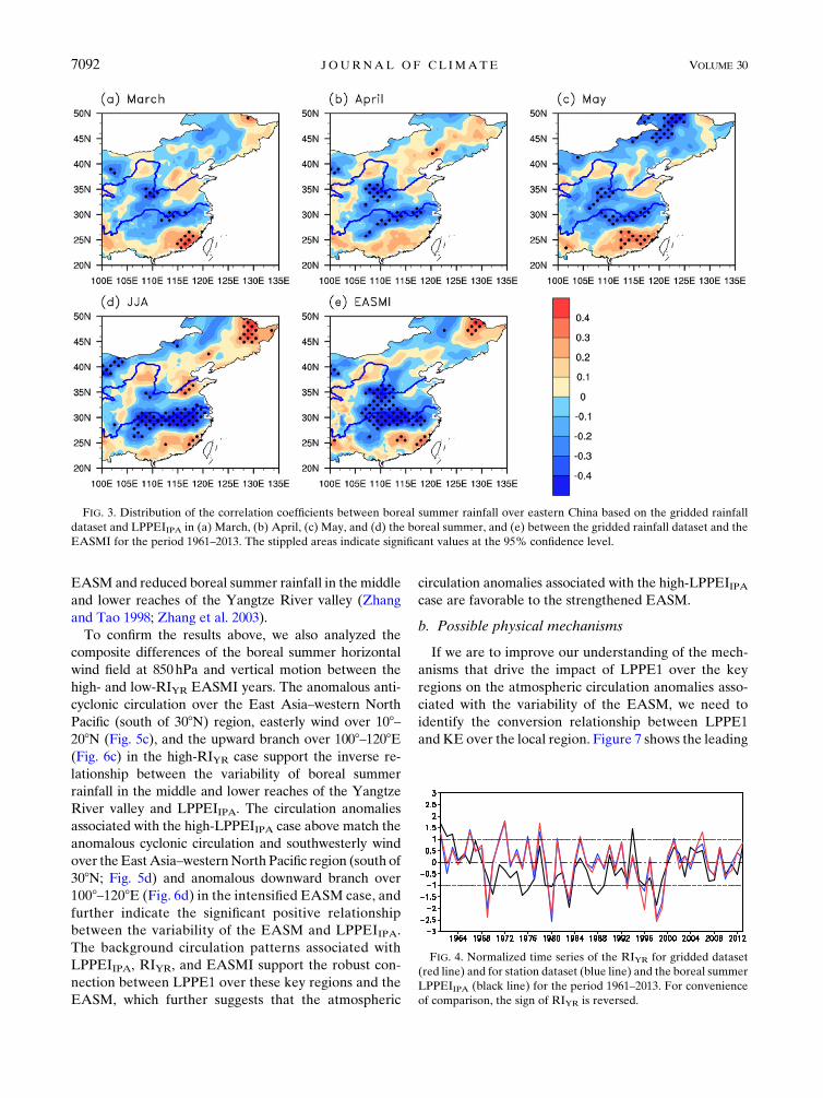
Figure 3 displays the correlation distributions be-

tween LPPEIIPA and boreal summer rainfall over east-

ern China using the gridded precipitation dataset. There

are negative values (the stippled areas) in the middle

and lower reaches of the Yangtze River valley (Figs. 3a–

d), which are consistent with the relationship between

the EASMI and boreal summer rainfall (Fig. 3e). To

ensure the robustness of the results, we also used the

China 160-station precipitation dataset. The significant

negative correlations between LPPEIIPA from preceding

March to the boreal summer and boreal summer pre-

cipitation in the middle and lower reaches of the

Yangtze River valley (not shown) coincide with the re-

sults presented in Fig. 3. These results further confirm

that the anomalies of LPPE1 over the eastern Indian

Ocean, subtropical central Pacific, and East Asia regions

are closely connected with the variability of the EASM.

To highlight the connection between LPPE1 over the

key regions and boreal summer rainfall in the middle

and lower reaches of the Yangtze River valley, we

define a rainfall index that is the time series of boreal

summer rainfall averaged over the significantly corre-

lated area 28.258–31.258N, 106.758–118.258E denoted as

RIYR. Figure 4 shows the reversed relationship between

RIYR and LPPEIIPA during the boreal summer, with a

correlation coefficient of 20.56 based on the gridded

dataset; for the station dataset, the value is 20.52 (both

significant at the 99.9% confidence level). This also

demonstrates the consistency of the two rainfall datasets

used here. In the following discussion, the RIYR time

series is based on the boreal summer gridded pre-

cipitation dataset.

4. Connections between LPPE1 over the keyregions and the EASM

a. Boreal summer atmospheric circulation anomaliesover East Asia associated with LPPEIIPA

We used composite analysis to examine the close

connection between the EASM and LPPE1 over the

three key regions and explore the boreal summer atmo-

spheric circulation anomalies associated with LPPEIIPA.

To examine the stable influence of LPPEIIPA on the

EASM, we also analyze the circulation anomalies cor-

responding to the preceding LPPEIIPA; here we mainly

give the composite differences of atmospheric circula-

tion patterns associated with LPPEIIPA in May and

boreal summer. Figure 5 displays the composite differ-

ences of the boreal summer horizontal wind field at

850 hPa between the high- and low-LPPEIIPA years. The

results show that there is an anomalous cyclonic circu-

lation and southwesterly wind over East Asia (south of

308N), and an anomalous westerly wind over 108–208N,

implying stronger convection anomalies over the mon-

soon trough associated with the high-LPPEIIPA values

in both May (Fig. 5a) and the boreal summer (Fig. 5b).

Figure 6 presents the composite differences of the boreal

summer vertical motion along 258–358N between the

high- and low-LPPEIIPA years. There are downward

motion anomalies within 1008–1208E, indicating that

there is weaker convective activity over the mei-yu

front, and anomalous downward motion in the middle

and lower reaches of the Yangtze River valley in the

high-LPPEIIPA case (Figs. 6a,b). The circulation anom-

alies in the high-LPPEIIPA case are coincident with the

characteristics of background atmospheric circulation

patterns over East Asia associated with the intensified

FIG. 2. Normalized time series of the boreal summer LPPEIIPA(blue line) and the EASMI (red line) for the period 1948–2014. The

value of correlation coefficient (corr) between the time series is

provided at the top-right corner of the figure.

TABLE 1. Correlation coefficients between the LPPEIIPA and

EASMI for the period 1948–2014. The values in parentheses rep-

resent the 9-yr low-pass and high-pass time series, respectively,

which may represent the decadal and interannual components of

a variable. The correlation coefficients significant at the 99%

confidence level using the Student’s t test are in boldface. The

significance of the correlation between two low-pass time series

was assessed using the effective number of degrees of freedom

(Bretherton et al. 1999).

EASMI

LPPEIIPA in JJA 0.52 (0.64, 0.52)LPPEIIPA in May 0.41 (0.61, 0.39)

LPPEIIPA in April 0.52 (0.73, 0.48)

LPPEIIPA in March 0.47 (0.71, 0.39)

1 SEPTEMBER 2017 HUYAN ET AL . 7091

EASM and reduced boreal summer rainfall in the middle

and lower reaches of the Yangtze River valley (Zhang

and Tao 1998; Zhang et al. 2003).

To confirm the results above, we also analyzed the

composite differences of the boreal summer horizontal

wind field at 850hPa and vertical motion between the

high- and low-RIYR EASMI years. The anomalous anti-

cyclonic circulation over the East Asia–western North

Pacific (south of 308N) region, easterly wind over 108–208N (Fig. 5c), and the upward branch over 1008–1208E(Fig. 6c) in the high-RIYR case support the inverse re-

lationship between the variability of boreal summer

rainfall in the middle and lower reaches of the Yangtze

River valley and LPPEIIPA. The circulation anomalies

associated with the high-LPPEIIPA case above match the

anomalous cyclonic circulation and southwesterly wind

over theEastAsia–westernNorth Pacific region (south of

308N; Fig. 5d) and anomalous downward branch over

1008–1208E (Fig. 6d) in the intensified EASM case, and

further indicate the significant positive relationship

between the variability of the EASM and LPPEIIPA.

The background circulation patterns associated with

LPPEIIPA, RIYR, and EASMI support the robust con-

nection between LPPE1 over these key regions and the

EASM, which further suggests that the atmospheric

circulation anomalies associated with the high-LPPEIIPAcase are favorable to the strengthened EASM.

b. Possible physical mechanisms

If we are to improve our understanding of the mech-

anisms that drive the impact of LPPE1 over the key

regions on the atmospheric circulation anomalies asso-

ciated with the variability of the EASM, we need to

identify the conversion relationship between LPPE1

andKE over the local region. Figure 7 shows the leading

FIG. 4. Normalized time series of the RIYR for gridded dataset

(red line) and for station dataset (blue line) and the boreal summer

LPPEIIPA (black line) for the period 1961–2013. For convenience

of comparison, the sign of RIYR is reversed.

FIG. 3. Distribution of the correlation coefficients between boreal summer rainfall over eastern China based on the gridded rainfall

dataset and LPPEIIPA in (a) March, (b) April, (c) May, and (d) the boreal summer, and (e) between the gridded rainfall dataset and the

EASMI for the period 1961–2013. The stippled areas indicate significant values at the 95% confidence level.

7092 JOURNAL OF CL IMATE VOLUME 30

SVD mode of boreal summer LPPE1 (Figs. 7a,c) and

KE (Figs. 7b,d), which explains 45% of the total co-

variance. The two time series are strongly correlated,

with a coefficient of 0.93 (significant at the 99.9% con-

fidence level). The LPPE1 field is characterized by a

positive phase in the tropical Indian Ocean and South

China Sea, and a negative phase in the subtropical

central Pacific and midlatitude East Asia. The KE field

has a negative phase in the tropical Indian Ocean, cen-

tral Pacific, and East Asia. With the high correlation

coefficient of the time series of LPPE1 and KE fields,

when there are negative LPPE1 anomalies in the trop-

ical Indian Ocean and positive LPPE1 anomalies in the

subtropical central Pacific and midlatitude East Asia,

then positive KE anomalies appear over the East Asia

region. These results suggest the coupled relationship

between LPPE1 over the key regions and KE over the

EASM region (108–408N, 1108–1408E), and also show

that there are positive KE anomalies over the EASM

region when there is a negative–positive–positive

LPPE1 pattern (2, 1, 1) over the eastern Indian

Ocean, subtropical central Pacific, and East Asia regions

(i.e., during the positive LPPEIIPA case).

In addition, the significant negative correlation over

the tropical Indian Ocean and midlatitude East Asia in

the LPPE1 field reflects the out-of-phase variations in

LPPE1 anomalies over the tropical and middle latitude

regions. The meridional out-of-phase pattern of LPPE1

may favor the meridional circulation adjustment in the

local area. Figure 8 shows the composite differences of

meridional circulation along 1108–1408E between the

high- and low-LPPEIIPA cases in May (Fig. 8a) and the

boreal summer (Fig. 8b). There is anomalous upward

motion over the north of the EASM region (408–508N)

and anomalous downward motion over the south of the

EASM region (08–108N), which implies that there is

anomalous convergence over 408–508N and divergence

over 08–108N. The anomalous vertical movement results

in anomalous southerlies at low levels, which then turn

right, under the influence of the Coriolis force, and this

can lead to strengthened southwesterly winds at low

levels and positive KE anomalies over the EASM re-

gion. These KE anomalies within the EASM system are

associated with a stronger EASM and anomalous

southwesterlies match the horizontal wind anomalies

over East Asia (south of 308N) at 850hPa in Figs. 5a,b.

The anomalous downward branch around 308N associ-

ated with the high-LPPEIIPA case is consistent with the

downward anomaly over 1008–1208E in Figs. 6a,b. The

above results indicate that the local meridional circula-

tion adjustment can influence the local circulation

anomalies over East Asia.

FIG. 5. Composite differences of the boreal summer winds at 850 hPa (vectors; m s21) between the high and low

LPPEIIPA in (a)May and (b) the boreal summer and between the high and low (c) RIYR and (d) EASMI years. The

light and dark shaded areas indicate anomalies significant at the 90% and 95% confidence levels, respectively, and

the red (blue) shading corresponds to westerly (easterly) wind.

1 SEPTEMBER 2017 HUYAN ET AL . 7093

We also present the composite differences of the

meridional circulation between the high- and low-RIYR

EASMI years. This shows an anomalous upward motion

over 08–108N and downward motion over 408–508N in

the high-RIYR case (Fig. 8c), which is the opposite pat-

tern to the high-LPPEIIPA case (Fig. 8a). The anomalous

downward (08–108N) and upward (408–508N) branches

associated with the high-LPPEIIPA case are consistent

with vertical movement anomalies during the intensified

EASM period (Fig. 8d). In addition, there is an anom-

alous downward branch with high LPPEIIPA, EASMI,

and anomalous upward motion around 308N with the

high RIYR. These results further prove the close con-

nection between LPPE1 over the eastern Indian Ocean,

subtropical central Pacific, and East Asia regions and

the variability of the EASM.

To verify the physical mechanisms that explain the

impact of the out-of-phase LPPE1 pattern over the

tropical Indian Ocean and midlatitude East Asia on

the local meridional circulation from the point of view of

energetics, we investigated the composite anomalies of

the boreal summer LPPE1 (regional zonal mean over

1108–1408E) based on the high- and low-LPPEIIPAyears. When LPPEIIPA is in its high phase, there are

negative LPPE1 anomalies over 08–108N and positive

LPPE1 anomalies over 408–508N (Fig. 9a). According to

PPE theory, the variability of LPPE1 can represent the

changes of the perturbation component of air temper-

ature. That is, when there are negative LPPE1 anoma-

lies over 08–108N and positive LPPE1 anomalies over

408–508N, the perturbation air is colder (warmer) over

08–108N (408–508N). Therefore, there is anomalous up-

ward branch associated with the warmer air and anom-

alous downward branch associated with the colder air,

LPPE1 converts to KE, and the vertical motion anom-

alies and local energy conversion can then induce the

anomalous meridional circulation as presented in

Fig. 8a. The situation for the negative LPPEIIPA case is

reversed (Fig. 9b), indicating that there is an anomalous

upward branch accompanying the warmer perturbation

air over 08–108N and an anomalous downward branch

with the colder perturbation air over 408–508N, which

can lead to the development of the local meridional

circulation pattern that is the opposite with those in the

high-LPPEIIPA case.

To further explore the coupled relationship between

the boreal summer LPPE1 and KE over the EASM re-

gion, we calculated the areal averaged LPPE1 and KE

FIG. 6. Composite differences of the boreal summer vertical velocity (1022 Pa s21) between the high and low

LPPEIIPA in (a) May and (b) the boreal summer and between the high and low (c) RIYR and (d) EASMI years.

Contours show the composite differences and the contours22.0,20.5, 0, 0.5, and 2.03 1022 Pa s21 are given. The

light and dark shaded areas indicate anomalies significant at the 90% and 95% confidence levels, respectively, and

the red (blue) shading corresponds to upward (downward) motion. The longitude–pressure cross sections are along

258–358N, and the y axis is pressure (hPa).

7094 JOURNAL OF CL IMATE VOLUME 30

over the EASM region based on the high- and low-

LPPEIIPA years. The area-averaged KE anomalies were

significantly positive (negative) in the high- (low-)

LPPEIIPA case, which were consistent with the positive

(negative) KE anomalies over the EASM region asso-

ciated with the high (low) LPPEIIPA and stronger

(weaker) EASM mentioned above. There were more

(fewer) area-averaged LPPE1 anomalies in the high-

(low-) LPPEIIPA case. The tendencies of the area-

averaged LPPE1 and KE over the EASM region in

the boreal summer (not shown) are positively correlated

(significant at the 99% confidence level), which shows

that when the variations of LPPE1 are positive over the

EASM region, the local KE is more likely to increase

and can indicate the positive relationship between the

variability of the area-averaged LPPE1 and KE over the

EASM region. Thereby, in the low-LPPEIIPA case,

there are fewer area-averaged LPPE1 anomalies com-

pared with those in the high-LPPEIIPA case, which in-

dicates that there is less energy over the EASM region

that could be transformed into the local KE. In addition,

because of the consistent relationship between the var-

iations of LPPE1 and KE over the EASM region, the

less LPPE1 anomalies can lead to reduced KE anoma-

lies during the low-LPPEIIPA case, which explains why

there are more (fewer) KE anomalies over the EASM

region during the high- (low-) LPPEIIPA case.

The results above suggest that the LPPE1 anomalies

over the key regions can cause atmospheric circulation

anomalies over East Asia via the meridional circulation

adjustment during the boreal summer, which is induced

by the out-of-phase variations in LPPE1 anomalies over

the north and south of the EASM regions based on the

PPE theory. The anomalous circulation patterns favor a

stronger (weaker) EASM and less (more) boreal sum-

mer rainfall in the middle and lower reaches of the

Yangtze River valley. The generation of LPPE1 anom-

alies over the key regions needs further investigation.

LPPE1 is closely related to the underlying external

forcing, the variability of which may be responsible for

the changes of LPPE1.

5. LPPE1 and the underlying external forcing

According to the derivation of the governing equation for

PPE1 (see details in appendix B),GL 5 g21Ð p2p1Q0 dp is the

source or sink term of LPPE1. Here, the perturbation

diabatic heating Q0 is the deviation from the spherical

average of the primitive diabatic heating Q, which in-

dicates the local variation of the diabatic heating.Besides,

according to Li and Gao (2006), PPE1 represents the

local energy conversion efficiency. Therefore, here we

applied the perturbation components of the variables to

investigate the contributions of underlying forcing over

the key regions on the changes of LPPE1.

Figure 10 presents the heterogeneous correlation pat-

terns of the leading SVD mode for the boreal summer

LPPE1 (Figs. 10a,c) and perturbation SST (Figs. 10b,d) in

FIG. 7. Correlation patterns for the leading SVD mode for (left) LPPE1 and (right) KE in the boreal summer.

Shown are heterogeneous correlationmaps representing (a),(b) the correlations between the expansion coefficients

of LPPE1 (KE) field and the gridpoint values of KE (LPPE1) field and (c),(d) the coefficients of the leading mode

to the time series of the LPPE1 (KE) field at each grid point. The contour interval is 0.2. The boxes in (b) and

(d) indicate the EASM region (108–408N, 1108–1408E). The light and dark shaded areas indicate significant values atthe 90% and 95% confidence levels, respectively.

1 SEPTEMBER 2017 HUYAN ET AL . 7095

May (Figs. 10a,b) and the boreal summer (Figs. 10c,d).

The SST pattern of the leading mode is significantly

correlated with the LPPE1 of the leading mode, with a

correlation coefficient of 0.86 for SST in boreal summer,

and for SST in May the value is 0.74 (both significant at

the 99.9% confidence level). When there are warmer

perturbation SSTs in the local region, positive LPPE1

anomalies appear in this area. The high correlation coeffi-

cients of the two time series indicate that LPPE1 increases

(decreases) accompany warmer (colder) perturbation

SST in the local region. The coupled relationship between

LPPE1 and perturbation SST over the key regions in-

dicates that the changes in the regional SST make a

positive contribution to the LPPE1 anomalies, and this

explains the role of local SST variability in the genera-

tion of LPPE1 over the key regions.

To provide a better understanding of the influence of

the local SST on the variability of LPPE1 over the key

regions, we focused on the local latent heat to analyze the

connection between the underlying diabatic heating and

FIG. 8. Composite differences of the boreal summermeridional circulation [vectors; meridional wind (m s21) and

vertical velocity (21022 Pa s21)] between the high and low LPPEIIPA in (a) May and (b) the boreal summer, and

between the high and low (c) RIYR and (d) EASMI years. The light and dark shaded areas indicate anomalies

significant at the 90% and 95% confidence levels, respectively, and the red (blue) shading corresponds to upward

(downward) motion. The latitude–pressure cross sections are along 1108–1408E, and the y axis is pressure (hPa).

FIG. 9. Meridional distributions of the composite of the boreal summer LPPE1 (regional

zonal mean over 1108–1408E; 106 Jm22) based on the (a) high- and (b) low-LPPEIIPA cases.

7096 JOURNAL OF CL IMATE VOLUME 30

the changes of LPPE1 over the key regions. As there are

both ocean and land signals in the East Asia region, here

we concentrate on the relationship between the variability

of LPPE1 and local latent heat in the eastern Indian

Ocean and subtropical central Pacific. Moreover, the

surface latent heat flux may not represent the total latent

heat release, so here we use the PWC to depict the latent

heating released by the condensation process. The ISCP is

highly related to the area-averaged perturbation PWC

over the subtropical central Pacific at a confidence level

greater than 99% (Fig. 11a). It can be seen that the IEIOand area-averaged perturbation PWC over the eastern

Indian Ocean are also significantly correlated (significant

at the 95% confidence level) (Fig. 11b). The significant

positive relationships between the perturbation PWC and

LPPE1 in the eastern Indian Ocean and subtropical cen-

tral Pacific indicate that the increases (decreases) of latent

heat release in the eastern Indian Ocean and subtropical

central Pacific lead to heating (cooling) of the air column,

resulting in more (fewer) LPPE1 anomalies in the eastern

IndianOcean and subtropical central Pacific. The positive

correlations also match the positive contribution of per-

turbation SST to the variability of LPPE1, which high-

lights the connection between the changes in local SST

and latent heat release. These results suggest that the

changes of local SST affect LPPE1 in the eastern Indian

Ocean and subtropical central Pacific by heating (cooling)

the atmosphere through local latent heat release.

According to Eqs. (5) and (6), we can see that the

underlying diabatic heating is contained in the source

term GL as in the right-hand side of Eq. (5). The

conversion term CK in both equations reflects the con-

version between LPPE1 and KE in the local scale. This

indicates that the contribution of external heating on the

local KE of circulation has to be accomplished through

the changes of LPPE1, and LPPE1 is the part that can be

directly transformed into the local KE around the

FIG. 10. Heterogeneous correlation patterns of the leading SVD mode for the (left) LPPE1 and (right) per-

turbation SST in (a),(b)May and (c),(d) boreal summer. The contour interval is 0.2. The light and dark shaded areas

indicate significant values at the 90% and 95% confidence levels, respectively. The percentages in red are the

explained variance of the leading mode.

FIG. 11. Normalized time series of the perturbation PWC over

the (a) subtropical central Pacific and (b) eastern Indian Ocean in

May (red lines) and the boreal summer (blue lines), and ISCP in

(a) and IEIO in (b) in the boreal summer (black lines) for the period

1948–2014. The correlation coefficients between the ISCP and PWC

over the subtropical central Pacific are 0.33 and 0.73 in May and

boreal summer, respectively, and the correlation coefficients be-

tween the IEIO and PWC over the eastern Indian Ocean are 0.30

and 0.42 in boreal summer and May, respectively.

1 SEPTEMBER 2017 HUYAN ET AL . 7097

EASM system from the underlying external heating

over the key regions. Then the variations of atmospheric

circulation anomalies over East Asia are correspon-

dences to the variations of the driving energy around the

EASM system, and thus influence the strength of the

EASM. Based on the above results, the close relation-

ship between SST in the Indian Ocean and the EASM

(Nan and Li 2005; Li et al. 2011a; G. Huang et al. 2016)

can be explained through the PPE theory as follows:

colder SST in the Indian Ocean basin can induce de-

creases of LPPE1, which means that there are negative

LPPE1 anomalies in the eastern Indian Ocean region

(i.e., the positive LPPEIIPA phase) and this favors a

stronger EASM and reduced boreal summer rainfall in

the middle and lower reaches of the Yangtze River

valley. This suggests that LPPE1 in the eastern Indian

Ocean may play a bridging role for the effects of the

local SST on the variability of the EASM.

6. Summary and discussion

In this article, we have demonstrated that the 1000–

850-hPa LPPE1 over three key regions (the eastern In-

dian Ocean, subtropical central Pacific, and East Asia)

has a robust connection with the EASM variability from

March to the boreal summer.We found that the positive

(negative) LPPEIIPA case—that is, the 2, 1, 1(1, 2, 2) LPPE1 pattern over the key regions—can

cause negative (positive) LPPE1 anomalies over the

south of the EASM region (08–108N) and positive

(negative) LPPE1 anomalies over the north of the

EASM region (408–508N). Based on the local energy

conversion and the PPE theory, we conclude that the

out-of-phase pattern of LPPE1 anomalies can lead to an

anomalous downward (upward) branch over 08–108N,

and an anomalous upward (downward) branch over 408–508N. The anomalous vertical movement induces the

local meridional circulation adjustment over East Asia.

The local meridional circulation anomalies then cause

an anomalous cyclonic (anticyclonic) circulation, a

southwesterly (northeasterly) wind over East Asia

(south of 308N) at 850 hPa, and an anomalous downward

(upward) branch over 1008–1208E (along 258–358N) in

the boreal summer, that can strengthen (weaken) the

EASM intensity, enhancing (reducing) KE over the

EASM region, and resulting in less (more) boreal sum-

mer rainfall in the middle and lower reaches of the

Yangtze River valley. We conclude that a warmer

(colder) local SST can induce more (less) LPPE1 in the

eastern Indian Ocean and subtropical central Pacific by

heating (cooling) the atmosphere via the increases (de-

creases) of local latent heat release. We mainly dis-

cussed the close connection between LPPE1 over the

three key regions and the EASM variability in view of

energetics. The results present that the related physical

processes are as follows: the changes of LPPE1 over the

key regions cause the variability of local KE within the

EASM system based on the local energy conversion.

The meridional circulation adjustment over East Asia

responds to the local energy conversion and anomalous

energy patterns. The local meridional circulation

anomalies then induce anomalous atmospheric circula-

tion and vertical motion over East Asia, leading to the

strengthened or weakened EASM.

Our results suggest that the LPPE1 signal over the key

areas could explain the physical processes and possible

mechanisms related to the underlying external forcing

transforming into KE of the EASM system, but could

also provide significant information that would help to

better predict the variability of the EASM. The physical

mechanisms and processes that explain the influence of

the changes of the underlying external forcing on

LPPE1 over the key regions require further exploration.

We should also consider the interaction between the

ocean and atmosphere, and the feedback between the

heat fluxes and the changes in SST. It can be seen that

there are significantly negative correlations over the

tropical Atlantic Ocean (Figs. 1a–d). We added LPPE1

over the Atlantic Ocean into the LPPEIIPA and

obtained a new LPPE1 index. The correlation co-

efficient between the EASMI and this new index has

been slightly increased in comparison to that with the

LPPEIIPA. The composite differences of atmospheric

circulation between high and low cases of the new index

(not shown) have not been significantly strengthened

compared with the anomalous circulation patterns as-

sociated with the LPPEIIPA case (Figs. 5a,b and 6a,b).

This indicates that the explained variation of the EASM

has not been highly improved with LPPE1 over the

Atlantic Ocean included, which also validates the sig-

nificant contributions of the three key regions on the

EASM variability we mostly discussed. Additionally,

the possible mechanisms that give rise to the anomalous

LPPE1 pattern over the eastern Indian Ocean, sub-

tropical Pacific, and East Asia regions remain unsolved.

We also found that LPPE1 over the key regions and the

EASM are both correlated on the interannual and de-

cadal time scales. We mostly investigated the relation-

ship between the EASM and LPPE1 over the key

regions on the interannual time scale, and more details

of the physical processes on the decadal time scale need

to be investigated in future work.

In this paper we mainly focused on summer rainfall

over eastern China; more research is needed to further

understand the intraseasonal modes of the EASM

rainfall (e.g., Oh and Ha 2015, 2016; Yim et al. 2015;

7098 JOURNAL OF CL IMATE VOLUME 30

Xing et al. 2016). Moreover, we mainly analyzed the

boreal summer mean component of the EASM vari-

ability from the energetic view. It is also suggested that

the subseasonality is one of the most predominant as-

pects of the interannual and decadal variability of the

East Asian climate (e.g., Ha et al. 2009; Yun et al. 2010).

Understanding the energy conversion within the EASM

system on the subseasonal time scale would aid to better

reveal the mechanisms on the EASM variability re-

sponding to the external conditions. All of these im-

portant issues will require further research.

Acknowledgments. This work was jointly supported

by the National Natural Science Foundation of China

(NSFC) Project 41530424 and SOA International Co-

operation Program on Global Change and Air–Sea In-

teractions (Grant GASI-IPOVAI-03). We sincerely

thank four anonymous reviewers for their constructive

comments and suggestions that helped to improve our

manuscript.

APPENDIX A

Dynamic Normalized Seasonality Index

The unified DNS monsoon index defined by Li and

Zeng (2002, 2003) is based on the intensity of wind field

seasonality and can be applied to describe both the

seasonal cycle and interannual variability of monsoons

over different domains. The DNS index is given by

dm,n

5kV

12V

m,nk

kVk 2 2, (A1)

where V1 is the January climatology wind vector, V is

the average of the January and July climatological wind

vectors, and Vm,n denotes the monthly wind vector in

themth month of the nth year; note that 2 is subtracted

on the right-hand side of Eq. (A1) because the critical

value of significant kV1 2Vm,nk/kVk is 2 (Li and

Zeng 2000).

APPENDIX B

TheDerivation of Perturbation Potential Energy andthe Governing Equations for Perturbation Potential

Energy and Kinetic Energy

a. Derivation of perturbation potential energy

The concept of PPE was first introduced by Li and

Gao (2006), the formal derivation of which (Li and Gao

2006) is given below.

The total potential energy (TPE; Margules 1903) of

the air column per unit area using the isentropic co-

ordinate system (l, f, u, t) can be written as

P51

(11 k)gdpk00

ðutus

p11k du11

(11k)gdpk00

usp11ks 1z

sps,

(B1)

where zs 5 zs(l, f) is the surface topography; l and

f are the longitude and latitude, respectively; p is

pressure; ps 5 ps(l, f) is surface pressure; g is the

gravitational acceleration; cp5 cy1R is the specific heat

at constant pressure, where R is the gas constant for dry

air, and cy is the specific heat at constant volume; and

gd 5 g/cp is the dry adiabatic lapse rate. Also, T is

temperature; u5 T(p00/p)k is potential temperature and

k 5 R/cp; us and ut are potential temperatures at zs and

the top of tropopause, respectively; and p00 is the ref-

erence pressure (usually taken as 1000hPa). The con-

cept of APE (Lorenz 1955) is based on the mass

conservation and on the redistribution of the atmo-

sphere into the reference state through isentropic

processes.

The difference of the TPE between the actual state

and the reference state through adiabatic redistribution

is

P 0 5P2 ~P5P 0a 1P 0

s , (B2)

where the tilde indicates physical variables in the ref-

erence state, Pa is the portion related to the air column,

and Ps is the portion related to the surface topography;

P 0a 5Pa 2 ~Pa, P

0s 5Ps 2 ~Ps, and P 0 is made of two parts:

the first part is related to the air column and is called the

atmospheric perturbation potential energy (shortened

to PPE), and the second part is related to topography

and is called the surface perturbation potential energy

(SPPE). Gao et al. (2006) showed that the potential

temperatures at the boundary are invariant (~ut 5 ut,~us 5 us) through isentropic processes under the condi-

tion of conservation of mass. We obtain the expressions

for the PPE and SPPE:

P 0a 5

1

(11 k)gdpk00

ðutus

(p11k 2 ~p11k) du and (B3)

P 0s 5

1

(11k)gdpk00

us(p11k

s 2 ~p11ks )1 z

s(p

s2 ~p

s) . (B4)

Because the atmosphere is integrated as a whole, its

adiabatic redistribution can only be accomplished on the

global rather than the local scale. Therefore, the above-

mentioned reference state is defined as the spherical

averaged on isentropic surfaces ~p5 p(u).

1 SEPTEMBER 2017 HUYAN ET AL . 7099

We derive the formula in isobaric coordinates to

facilitate practical computation. Only the atmospheric

PPE is considered here. It is convenient to partition

the total pressure field into two parts: standard

pressure, which is the spherically averaged pressure on

isentropic surfaces, and pressure perturbations from

the standard values, so p5 p1 p0. Then Eq. (B3) can be

written as

P 0a 5 �

‘

i51

P 0ai 5

1

gdpk00

ðutus

p11k

"p0

p1

k

2

�p0

p

�2

1k(k2 1)

3!

�p0

p

�3

1⋯

#du , (B5)

where P 0ai (for i 5 1, 2, . . .) depends on the power of

perturbation pressure p0i, and is called the ordinal-order

moment term of PPE. According to Lorenz (1955), the

perturbation pressure p0 on an isentropic surface and the

perturbation potential temperature u0 on an isobaric

surface can be approximated p0(u)’2u0›p/›u.The expression of ordinal-order moment term of PPE

in isobaric coordinate system can be written as

P0ai 5Pi21

j50

(11 k2 j)

i!gd(11 k)pk

00

ðps0

p11k2iu0i�2›u

›p

�2i11

dp . (B6)

Making use of the relation between the perturbation po-

tential temperature and perturbation temperature, u0/u5T 0/T and u0 5T 0(p00/p)

k; then Eq. (B6) can be given by

P 0ai 5

p(i21)k00 P

i21

j50

(11 k2 j)

i!gd(11 k)

ðps0

T 0i

p(i21)(11k)

�2›u

›p

�2i11

dp .

(B7)

The PPE1 and PPE2 are expressed as

P 0a1 5

1

gd

ðps0

T 0 dp and (B8)

P 0a2 5

kpk00

2gd

ðps0

T 02

p11k

�2›u

›p

�21

dp . (B9)

Actually, high-order moment terms of PPE are much

smaller comparedwith PPE1 andPPE2 and can be omitted.

b. Derivation of governing equations for perturbationpotential energy and kinetic energy

Wang et al. (2012) introduced the governing equa-

tions for PPE1 and KE.

Using the isobaric spherical coordinate system (l,f, u, t),

the fundamental equations for the atmosphere (Peixoto and

Oort 1992; see their chapter 14) can be written as

du

dt2

1

auy tanf52

1

a cosf

›u›l

1 f y1 gl, (B10)

dy

dt1

1

au2 tanf52

1

a

›u›f

2 fu1 gf, (B11)

›u›p

52RT

P, (B12)

1

a cosf

�›u

›l1

›y cosf

›f

�1

›v

›p5 0, (B13)

cp

dT

dt2av5Q , (B14)

where d/dt5 ›/›t1 (a cosf)21u›/›l1 a21y›/›f1v›/›p,

a is the mean radius of Earth, Vh 5 ui1 yj is the hori-

zontal velocity vector, v 5 dp/dt is the vertical velocity,

D3B5 (a cosf)21[›Bi/›l1 ›(Bj cosf)/›f]1 ›Bk/›p is

the divergence operator, u is the gravitational potential,

gh 5 gli1 gfj is the horizontal friction force, a 5 r21 is

specific volume, R is the gas constant of dry air, cp is the

specific heat at constant pressure, T is temperature, Q is

diabetic heating, f 5 2V sinf is the acceleration by the

Coriolis force, V is the angular velocity of Earth’s rota-

tion, and =h 5 (a cosf)21›/›li1 a21›/›fj is the hori-

zontal gradient operator.

We use ( )5 (4pa2)21Ð p/22p/2

Ð 2p0 ( )a2 cosf dl df to de-

fine the spherical average. The primitive variable

is then ( )5 ( )1 ( )0, where the prime designates the

deviation from the spherical average. Assuming

that the physical variable consists of spherical-averaged

and perturbation components: F(l, f, p, t)5F(p, t)1F 0(l, f, p, t), we then have

1

a cosf

›F

›l5 0,

1

a

›F

›f5 0,

1

a cosf

›F

›l5 0,

1

a

›F

›f5

1

aF tanf ,

1

a cosf

›F cosf

›f52

1

aF tanf, and

1

a cosf

›F cosf

›f5 0.

(B15)

Applying the separation F(l, f, p, t)5F(p, t)1F 0(l, f, p, t) to the Eq. (B14), using identity Eq. (B15),

we obtain the perturbation part of the thermodynamic

equation:

7100 JOURNAL OF CL IMATE VOLUME 30

dcpT 0

dt52v

›u0

›p1

v0›u

0

›p2v0›u

›p

!1Q0

1

›c

pT 0v0

›p2v0›cpT

›p

!. (B16)

TheKE equation derived from the Eqs. (B10) and (B11)

can then be written as

›ek

›t1D

2(V

hek)1

›vek

›p

52D2(V

hu0)2

›vu0

›p1v

›u0

›p1V

hgh, (B17)

where ek 5 0:5(u2 1 y2) and A01 5 cpT

0.Integrating Eqs. (B16) and (B17) vertically over the

pressure, the governing equations of PPE1 and KE can

be given by

›

›tPPE15J

L1ℵ

L1R

L2C

K1G

Land (B18)

›

›tKE5B

K1<

K1C

K1M

K, (B19)

where PPE15 g21Ð ps0cpT

0 dp (Li and Gao 2006), KE5g21Ð ps0ek dp is kinetic energy, andCK 5 g21

Ð ps0v(›u0/›p) dp

is the conversion term between PPE1 and KE, which de-

pends on vertical velocity and atmospheric stability.When

CK is positivewithwarm (cold) air ascending (descending),

then PPE1 converts toKE; whenCK is negativewithwarm

(cold) air descending (ascending), KE converts to PPE1.

Also,GL 5 g21Ð ps0Q0 dp is the source (sink) term of PPE1;

when it gives net heating, PPE1will increase, whereas with

net cooling, PPE1will decrease.Uniformheating increases

the total energy but not the PPE1. The horizontal di-

vergence term is JL 52g21D2

Ð ps0VhA

01 dp, and ℵL 5

2g21(gvA01 1 cpT 0v0)ps is related to surface verticalmotion.

Furthermore, RL 52g21Ð ps0 [v

0›(cpT)/›p1v0›u/›p2v0›u0/›p]dp is related to the vertical redistribution of

temperature; MK 5 g21Ð ps0Vhgh dp is related to viscous

dissipation,withVh thehorizontal velocity vector andgh the

horizontal friction force;BK 52g21D2

Ð ps0Vh(u0 1 ek) dp is

related to transport and work by horizontal boundary

pressure; and <K 52g21[v(ek 1u0)]ps is related to topo-

graphic effects.

REFERENCES

Bretherton, C. S., M. Widmann, V. P. Dymnikov, J. M.

Wallace, and I. Bladé, 1999: The effective number of

spatial degrees of freedom of a time-varying field.

J. Climate, 12, 1990–2009, doi:10.1175/1520-0442(1999)012,1990:

TENOSD.2.0.CO;2.

Bullock, B. R., and D. R. Johnson, 1971: The generation of available

potential energy by latent heat release in a mid-latitude cyclone.

Mon.Wea. Rev., 99, 1–14, doi:10.1175/1520-0493(1971)099,0001:

TGOAPE.2.3.CO;2.

Ding, R. Q., K.-J. Ha, and J. P. Li, 2010: Interdecadal shift in the

relationship between the East Asian summer monsoon and

the tropical Indian Ocean. Climate Dyn., 34, 1059–1071,

doi:10.1007/s00382-009-0555-2.

Dong, D., J. P. Li, L. D. Huyan, and J. Q. Xue, 2017: Atmospheric

energetics over the tropical Pacific during the ENSO cycle.

J. Climate, 30, 3635–3654, doi:10.1175/JCLI-D-16-0480.1.

Feng, J., J. P. Li, and Y. Li, 2010: A monsoon-like southwest

Australian circulation and its relation with rainfall in south-

west Western Australia. J. Climate, 23, 1334–1353,

doi:10.1175/2009JCLI2837.1.

Gao, L., and J. P. Li, 2007: Progress in the study of atmospheric

energy efficiency (in Chinese). Adv. Earth Sci., 22, 486–494.

——, and ——, 2012: Relationship and mechanism between per-

turbation potential energy and atmospheric general circula-

tion anomalies. Chin. J. Geophys., 55, 359–374, doi:10.1002/

cjg2.1730.

——, and ——, 2013: Impacts and mechanism of diabatic heating

on atmospheric perturbation potential energy (in Chinese).

Chin. J. Geophys., 56, 3255–3269.

——, ——, and H. L. Ren, 2006: Some characteristics of the at-

mosphere during an adiabatic process (in Chinese). Prog. Nat.

Sci., 16, 243–247.

Gu, X. Z., 1990: A theoretical study of the available potential en-

ergy in a limited atmospheric region (in Chinese). Acta Me-

teor. Sin., 48, 248–252.

Guan, Z. Y., 2000: The variations of Asian monsoon as revealed by

the variations of kinetic energy of barotropic/baroclinicmodes

of the wind field (in Chinese). J. Nanjing Inst. Meteor., 23, 313–

322.

Guo, Q. Y., and J. Q.Wang, 1986: The snow cover on Tibet Plateau

and its effect on the monsoon over East Asia (in Chinese).

Plateau Meteor., 5, 116–124.

Ha, K.-J., K.-S. Yun, J.-G. Jhun, and J. P. Li, 2009: Circulation

changes associated with the interdecadal shift of Korean Au-

gust rainfall around late 1960s. J. Geophys. Res., 114, D04115,

doi:10.1029/2008JD011287.

He, J. H., J. J. Yu, X. Y. Shen, and H. Gao, 2004: Research on

mechanism and variability of East Asian monsoon (in Chi-

nese). J. Trop. Meteor., 20, 449–459.

——, M. Wen, Y. H. Ding, and R. H. Zhang, 2006: Possible

mechanism for the impact of convection over Asia–

Australian ‘‘land bridge’’ on the establishment of East

Asian summer monsoon (in Chinese). Sci. China Earth Sci.,

36, 959–967.Huang, B. Y., and Coauthors, 2015: Extended Reconstructed Sea

Surface Temperature version 4 (ERSST.v4): Part I. Upgrades

and intercomparisons. J. Climate, 28, 911–930, doi:10.1175/

JCLI-D-14-00006.1.

——, and Coauthors, 2016: Further exploring and quantifying un-

certainties for Extended Reconstructed Sea Surface Tem-

perature (ERSST) version 4 (v4). J. Climate, 29, 3119–3142,

doi:10.1175/JCLI-D-15-0430.1.

Huang, G., K. M. Hu, X. Qu, W. C. Tao, S. L. Yao, G. J. Zhao, and

W. P. Jiang, 2016: A review about Indian Ocean basin mode

and its impacts on East Asian summer climate (in Chinese).

Chin. J. Atmos. Sci., 40, 121–130.

Huang, R. H., G. Huang, and B. H. Ren, 1999: Advances and

problems needed for further investigation in the studies of the

East Asian summer monsoon (in Chinese). Chin. J. Atmos.

Sci., 23, 129–141.

1 SEPTEMBER 2017 HUYAN ET AL . 7101

Johnson, D. R., 1970: The available potential energy of storms.

J.Atmos. Sci., 27, 727–741, doi:10.1175/1520-0469(1970)027,0727:

TAPEOS.2.0.CO;2.

Kalnay, E., and Coauthors, 1996: The NCEP/NCAR 40-Year Re-

analysis Project. Bull. Amer. Meteor. Soc., 77, 437–471,

doi:10.1175/1520-0477(1996)077,0437:TNYRP.2.0.CO;2.

Kang, I.-S., and Coauthors, 2002: Intercomparison of the climato-

logical variations of Asian summer monsoon precipitation

simulated by 10 GCMs. Climate Dyn., 19, 383–395, doi:10.1007/

s00382-002-0245-9.

Lau, N. C., and M. J. Nath, 2000: Impact of ENSO on the vari-

ability of the Asian–Australian monsoons as simulated in

GCM experiments. J. Climate, 13, 4287–4309, doi:10.1175/

1520-0442(2000)013,4287:IOEOTV.2.0.CO;2.

Li, C. Y., andM.Q.Mu, 1998: Numerical simulations of anomalous

winter monsoon in East Asia exciting ENSO (in Chinese).

Chin. J. Atmos. Sci., 22, 481–490.——, J.-T. Wang, S.-Z. Lin, and H.-R. Cho, 2004: The relationship

between East Asian summer monsoon activity and northward

jump of the upper westerly jet location (in Chinese). Chin.

J. Atmos. Sci., 28, 641–658.

Li, J. P., and Q. C. Zeng, 2000: Significance of the normalized sea-

sonality of wind field and its rationality for characterizing the

monsoon. Sci. China, 43D, 646–653, doi:10.1007/BF02879509.

——, and ——, 2002: A unified monsoon index. Geophys. Res.

Lett., 29, 1274, doi:10.1029/2001GL013874.

——, and ——, 2003: A new monsoon index and the geographical

distribution of the global monsoons.Adv. Atmos. Sci., 20, 299–

302, doi:10.1007/s00376-003-0016-5.

——, and ——, 2005: A new monsoon index, its interannual vari-

ability and relation with monsoon precipitation (in Chinese).

Climatic Environ. Res., 10, 351–365.

——, and L. Gao, 2006: Theory on perturbation potential energy

and its applications—Concept, expression and spatio-

temporal structures of perturbation potential energy (in Chi-

nese). Chin. J. Atmos. Sci., 30, 834–838.

——, Z. W. Wu, Z. H. Jiang, and J. H. He, 2010: Can global

warming strengthen the East Asian summer monsoon?

J. Climate, 23, 6696–6705, doi:10.1175/2010JCLI3434.1.

——, G. X. Wu, and D. X. Hu, 2011a: Ocean–Atmosphere In-

teraction over the Joining Area of Asia and Indian–Pacific

Ocean and Its Impact on the Short-Term Climate Variation

in China (in Chinese). Vol. 1. China Meteorological Press,

516 pp.

——, ——, and ——, 2011b: Ocean–Atmosphere Interaction over

the Joining Area of Asia and Indian–Pacific Ocean and Its

Impact on the Short-Term Climate Variation in China (in

Chinese). Vol. 2. China Meteorological Press, 565 pp.

——, and Coauthors, 2013: Progress in air–land–sea interactions in

Asia and their role in global and Asian climate change (in

Chinese). Chin. J. Atmos. Sci., 37, 518–538.——, S. Zhao, Y. J. Li, L. Wang, and C. Sun, 2016: On the role of

perturbation potential energy in variability of the East Asian

summer monsoon: Current status and prospects (in Chinese).

Adv. Earth Sci., 31, 115–125.

Liang, J. Y., and S. S. Wu, 2003: The study on the mechanism of

SSTA in the Pacific Ocean affecting the onset of summer

monsoon in the South China Sea—Numerical experiments (in

Chinese). Acta Oceanol. Sin., 25, 28–41.

Liu, W., and Coauthors, 2015: Extended Reconstructed Sea Sur-

face Temperature version 4 (ERSST.v4): Part II. Parametric

and structural uncertainty estimations. J. Climate, 28, 931–951,

doi:10.1175/JCLI-D-14-00007.1.

Lorenz, E. N., 1955: Available potential energy and the mainte-

nance of the general circulation. Tellus, 7, 157–167,

doi:10.3402/tellusa.v7i2.8796.

Margules, M., 1903: Über die Energie der Stürme. Jahrb. Zen-

tralanstalt Meteor. Geodyn., 40, 1–26.

Nan, S. L., and J. P. Li, 2005: The relationship between the summer

precipitation in the YangtzeRiver valley and the boreal spring

SouthernHemisphere annularmode: II. The role of the Indian

Ocean and South China Sea as an ‘‘oceanic bridge’’ (in Chi-

nese). Acta Meteor. Sin., 63, 849–856.

Oh, H., and K.-J. Ha, 2015: Thermodynamic characteristics and

responses to ENSO of dominant intraseasonal modes in the

East Asian summer monsoon. Climate Dyn., 44, 1751–1766,

doi:10.1007/s00382-014-2268-4.

——, and ——, 2016: Predictability of the dominant intraseasonal

modes in the East Asia–western North Pacific summer mon-

soon region. Climate Dyn., 47, 2025–2037, doi:10.1007/

s00382-015-2948-8.

Peixoto, J. P., and A. H. Oort, 1992: Physics of Climate. American

Institute of Physics, 520 pp.

Qian, W. H., 2005: Review of variations of the summer monsoon

from seasonal to interannual and interdecadal scales (in Chi-

nese). J. Trop. Meteor., 20, 1371–1386.

Song, F. F., and T. J. Zhou, 2014: Interannual variability of East

Asian summer monsoon simulated by CMIP3 and CMIP5

AGCMs: Skill dependence on Indian Ocean–western Pacific

anticyclone teleconnection. J. Climate, 27, 1679–1697,

doi:10.1175/JCLI-D-13-00248.1.

Tao, S. Y., and L. T. Chen, 1987: A review of recent research on the

East Asian summer monsoon in China. Monsoon Meteorol-

ogy, C. P. Chang, and T. N. Krishnamurti, Eds., Oxford Uni-

versity Press, 60–92.

van Mieghem, J., 1973: Atmospheric Energetics. Clarendon Press,

306 pp.

Wallace, J. M., C. Smith, and C. S. Bretherton, 1992: Singular value

decomposition of wintertime sea surface temperature and

500-mb height anomalies. J. Climate, 5, 561–576, doi:10.1175/

1520-0442(1992)005,0561:SVDOWS.2.0.CO;2.

Wang, B., LinHo, Y. S. Zhang, and M.-M. Lu, 2004: Definition of

South China Sea monsoon onset and commencement of the

East Asian summer monsoon. J. Climate, 17, 699–710,

doi:10.1175/2932.1.

——, Q. H. Ding, X. H. Fu, I.-S. Kang, K. Jin, J. Shukla, and

F. Doblas-Reyes, 2005: Fundamental challenge in simulation

and prediction of summer monsoon rainfall. Geophys. Res.

Lett., 32, L15711, doi:10.1029/2005GL022734.

——, Z. W.Wu, J. P. Li, J. Lin, C.-P. Chang, Y. H. Ding, and G. X.

Wu, 2008a: How to measure the strength of the East Asian

summer monsoon? J. Climate, 21, 4449–4463, doi:10.1175/

2008JCLI2183.1.

——, J. Yang, T. J. Zhou, and B. Wang, 2008b: Interdecadal

changes in the major modes of Asian–Australian monsoon

variability: Strengthening relationship with ENSO since the

late 1970s. J. Climate, 21, 1771–1789, doi:10.1175/

2007JCLI1981.1.

Wang, L., J. P. Li, and Y. Guo, 2012: Governing equations of

atmospheric layer perturbation potential energy and its

applications—Energy budget of the South China Sea summer

monsoon activity (in Chinese). Chin. J. Atmos. Sci., 36, 769–783.

——, ——, and R. Q. Ding, 2013: Theory on layer perturbation

potential energy and its application: A case study on annual

variation of the South China Sea summer monsoon (in Chi-

nese). Chin. J. Geophys., 56, 392–408.

7102 JOURNAL OF CL IMATE VOLUME 30

——,——,Z.G.Wang,Y. J. Li, and F. Zheng, 2015: The oscillation

of the perturbation potential energy between the extratropics

and tropics in boreal winter. Atmos. Sci. Lett., 16, 119–126,

doi:10.1002/asl2.532.

Wu, G. X., J. Y. Mao, A. M. Duan, and Q. Zhang, 2004: Recent

progress in the study of the impacts of Tibetan Plateau on

Asian summer climate (in Chinese). Acta Meteor. Sin., 62,

528–540.

——, Y. M. Liu, X. Liu, A. M. Duan, and X. Y. Liang, 2005: How

the heating over the Tibetan Plateau affects the Asian climate

in summer (in Chinese). Chin. J. Atmos. Sci., 29, 47–56.

Xing, W., B. Wang, and S.-Y. Yim, 2016: Peak-summer East Asian

rainfall predictability and prediction part I: Southeast Asia.

Climate Dyn., 47, 1–13, doi:10.1007/s00382-014-2385-0.

Yang, X. Q., Q. Xie, Y. M. Zhu, X. G. Sun, and Y. J. Guo, 2005:

Decadal-to-interdecadal variability of precipitation in North

China and associated atmospheric and oceanic anomaly pat-

terns (in Chinese). Chin. J. Geophys., 48, 789–797.

Yim, S.-Y., B. Wang, W. Xing, and M.-M. Lu, 2015: Prediction of

Meiyu rainfall inTaiwanbymulti-lead physical–empiricalmodels.

Climate Dyn., 44, 3033–3042, doi:10.1007/s00382-014-2340-0.

Yun, K.-S., K.-J. Ha, and B. Wang, 2010: Impacts of tropical ocean

warming on East Asian summer climate. Geophys. Res. Lett.,

37, L20809, doi:10.1029/2010GL044931.

Zhang, Q. Y., and S. Y. Tao, 1998: Tropical and subtropical mon-

soon over East Asia and its influence on the rainfall over

eastern China in summer (in Chinese).Quart. J. Appl.Meteor.,

9, 17–23.

——, ——, and L. T. Chen, 2003: The inter-annual variability of

East Asian summer monsoon indices and its association with

the pattern of general circulation over East Asia (in Chinese).

Acta Meteor. Sin., 61, 559–568.

Zhang, R. H., and Q. Li, 2004: Impact of sea temperature vari-

ability of tropical oceans on East Asianmonsoon (in Chinese).

Meteor. Mon., 30, 22–26.

Zhao, Y. F., and J. Zhu, 2015: Assessing quality of grid daily pre-

cipitation datasets in China in recent 50 years (in Chinese).

Plateau Meteor., 34, 50–58.——, ——, and Y. Xu, 2014: Establishment and assessment of the

grid precipitation datasets in China for recent 50 years (in

Chinese). J. Meteor. Sci., 34, 414–420.Zheng, J. Y., J. P. Li, and J. Feng, 2014: A dipole pattern in the

Indian and Pacific Oceans and its relationship with the East

Asian summer monsoon. Environ. Res. Lett., 9, 074006,

doi:10.1088/1748-9326/9/7/074006.

Zhu, C. W., X. J. Zhou, P. Zhao, L. X. Chen, and J. H. He, 2011:

Onset of East Asian sub-tropical summer monsoon and rainy

season in China. Sci. China Earth Sci., 54, 1845–1853,

doi:10.1007/s11430-011-4284-0.

Zuo, Z. Y., and R. H. Zhang, 2016: Influence of soil moisture in

eastern China on the East Asian summer monsoon. Adv. At-

mos. Sci., 33, 151–163, doi:10.1007/s00376-015-5024-8.

1 SEPTEMBER 2017 HUYAN ET AL . 7103