the impact of indian job guarantee scheme on labor market ...ftp.iza.org/dp6548.pdf · unemployment...

DI

SC

US

SI

ON

P

AP

ER

S

ER

IE

S

Forschungsinstitut zur Zukunft der ArbeitInstitute for the Study of Labor

The Impact of Indian Job Guarantee Scheme on Labor Market Outcomes:Evidence from a Natural Experiment

IZA DP No. 6548

May 2012

Mehtabul Azam

The Impact of Indian Job Guarantee Scheme

on Labor Market Outcomes: Evidence from a Natural Experiment

Mehtabul Azam World Bank

and IZA

Discussion Paper No. 6548 May 2012

IZA

P.O. Box 7240 53072 Bonn

Germany

Phone: +49-228-3894-0 Fax: +49-228-3894-180

E-mail: [email protected]

Any opinions expressed here are those of the author(s) and not those of IZA. Research published in this series may include views on policy, but the institute itself takes no institutional policy positions. The Institute for the Study of Labor (IZA) in Bonn is a local and virtual international research center and a place of communication between science, politics and business. IZA is an independent nonprofit organization supported by Deutsche Post Foundation. The center is associated with the University of Bonn and offers a stimulating research environment through its international network, workshops and conferences, data service, project support, research visits and doctoral program. IZA engages in (i) original and internationally competitive research in all fields of labor economics, (ii) development of policy concepts, and (iii) dissemination of research results and concepts to the interested public. IZA Discussion Papers often represent preliminary work and are circulated to encourage discussion. Citation of such a paper should account for its provisional character. A revised version may be available directly from the author.

mailto:[email protected]

IZA Discussion Paper No. 6548 May 2012

ABSTRACT

The Impact of Indian Job Guarantee Scheme on Labor Market Outcomes: Evidence from a Natural Experiment*

Public works programs, aimed at building a strong social safety net through redistribution of wealth and generation of meaningful employment, are becoming increasingly popular in developing countries. The National Rural Employment Guarantee Act (NREGA), enacted in August 2005, is one such program in India. This paper assesses causal impacts (Intent-to-Treat) of NREGA on public works participation, labor force participation, and real wages of casual workers by exploiting its phased implementation across Indian districts. Using nationally representative data from Indian National Sample Surveys (NSS) and Difference-in-Difference framework, we find that there is a strong gender dimension to the impacts of NREGA: it has a positive impact on the labor force participation and this impact is mainly driven by a much sharper impact on female labor force participation. Similarly, NREGA has a significant positive impact on the wages of female casual workers-real wages of female casual workers increased 8% more in NREGA districts compared with the increase experienced in non-NREGA districts. However, the impact of NREGA on wages of casual male workers has only been marginal (about 1%). Using data from pre-NREGA period, we also perform falsification exercise to demonstrate that the main conclusions are not confounded by pre-existing differential trends between NREGA and non-NREGA districts. JEL Classification: I38, O11, J21, J38 Keywords: difference-in-difference, intent-to-treat, NREGA, rural India Corresponding author: Mehtabul Azam World Bank 1818 H ST, NW MC7-712, Mail Stop: H11-1101 Washington, DC 20433 USA E-mail: [email protected]

* I would like to thank Mohamed Ihsan Ajwad, Basab Dasgupta, Sanjeev Kumar, Santosh Kumar, Daniel Millimet, Nishith Prakash, Tauhidur Rahman, and seminar participants at ECA-HDE, World Bank for helpful comments and discussion. Any error remains mine. The findings, interpretations, and conclusions expressed in this paper are entirely of the author and they do not necessarily represent the views of the World Bank.

mailto:[email protected]

1 Introduction

The notion that public works programs can build a strong social safety net through

redistribution of wealth and generation of meaningful employment has gained ground in

recent years. Many countries are increasingly adopting this strategy to tackle growing

unemployment and poverty.1 The National Rural Employment Guarantee Act (NREGA)

is a similar endeavor in India.2 NREGA was enacted during a time when more than a

decade of sustained high growth in GDP experienced in the 1980s and the 1990s was

perceived not to have made a sufficient dent in poverty in the rural India, leading to

euphemism of co-existence of two India(s): one, a thriving urban India and the other, a

stagnant rural India.

NREGA is a result of the Government of India’s stated principles of ‘inclusive growth’

and the desire to ensure that economic growth trickles down to the rural areas. When

NREGA was enacted in August 2005, there was optimism that the initiative would trans-

form rural India.3 NREGA entitles every rural household in India to a minimum of 100

days of paid work per year. This is an unrestricted entitlement with no eligibility re-

quirements. However, it was assumed that the nature of work under NREGA and the

wage rate would ensure that the program is self-targeted that attracts only the poor.

The primary objective of NREGA is to augment wage employment. Its secondary objec-

tive is to strengthen natural resource management through works that address causes of

chronic poverty like drought, deforestation and soil erosion and so encourage sustainable

development (Ministry of Rural Development, 2010).

NREGA was implemented in phases across rural India. In February 2006, it was

1Devereux and Solomon (2006) provide case studies for various country specific social safety netprograms.

2NREGA was renamed as Mahatma Gandhi National Rural Employment Guarantee Act (MGN-REGA) on October 2, 2009; however, in this paper we continue to use the old name.

3Based on their field investigation in two districts of Jharkhand, a state in India, Bhatia and Dreze(2006) report that NREGA has created a sense of hope amongst the rural poor and this sense of hope canbe further strengthened if people understand that the act gives them employment as a matter of right,and that claiming this right is within the realm of possibility.

1

launched in 200 backward districts in India. An additional 130 districts were covered

in year 2007-08 in the second Phase. The rest of the districts came under NREGA in

third Phase in year 2008-09 (Figure 1). The phase wise implementation ensured that

some districts remained uncovered during 2006-07 (Phase II and Phase III districts) and

during 2007-08 (Phase III districts). We exploit this phase wise expansion of NREGA

to evaluate the causal impacts (“Intent-to-Treat”) of NREGA on various outcomes of

interest such as participation in public work, labor force participation, and real wages of

casual workers using the difference-in-difference (DID) methodology.4’5 Using two rounds

of pre-program data, we also demonstrate that our main conclusions based on the DID

estimates are not confounded by the pre-program differential trends between NREGA and

non-NREGA districts.

The major findings of the paper are as follows. First, there has been a significant

increase in the public works participation in NREGA districts compared to the non-

NREGA districts. The increase in the share of public works in total casual labor has

been much higher for the female workers compared with the male workers or Scheduled

Caste/Tribe (SC/ST) workers. Second, NREGA has a positive impact on labor force

participation, and this impact is driven by a significant impact on the female labor force

participation. Post 2004-05, there has been a downward trend in labor force participation

in rural India. However, the positive impact of NREGA mitigated the situation in NREGA

districts compared to the non-NREGA districts. Third, NREGA has a positive impact

on average wages of casual workers; however, we find that this positive impact is driven

primarily by an increase in wages of female casual workers. The wages for female casual

4These outcomes are affected easily given any demand and supply shock. We would have liked to lookat the impacts of NREGA on the poverty and inequality; however, we could not implement our strategyfor these outcomes because of lack of comparable post program data (discussed in detail in Section 2).Similarly, we do not expect that NREGA will have a considerable impact on assets that raises landproductivity within couple of years, as these outcomes take time to materialize.

5Casual labor is defined as a person who has been casually engaged in others’ farm or non-farmenterprises (both household and non-household) and, in return, received wages according to the terms ofthe daily or periodic work contract. Casual workers are basically daily wage workers and the main targetgroup of NREGA.

2

workers increased 8 percent more in NREGA districts compared to the non-NREGA

districts. The impact of NREGA on male casual wages has been marginal (less than 1

percent increase). This suggests that the prevailing gender gaps in wages are reduced as

a result of NREGA.

The issue of NREGA pushing up the cost of agriculture is passionately debated in

Indian media. The argument forwarded against NREGA is that NREGA pushes up the

average wage of casual workers and distorts the agriculture labor markets.6 Our results

suggest that NREGA has only increased the wages of female casual worker. The existing

evidences suggest that female workers are paid much less than the statutory minimum

wages and wages paid to their male counterparts. Thus NREGA helped in reducing the

prevalent gender wage gap in casual works. One should see the increase in female wages as

success for NREGA as one of the objectives of such a program is to improve the conditions

and the bargaining power of the disadvantaged workers.

The paper proceeds as follows. In Section 1.1, we review the key facts and the existing

literature on NREGA. In Section 2, we describe the data, and we discuss the empirical

strategy in Section 3. Section 4 presents the results, and Section 5 concludes.

1.1 Background and Literature

NREGA is intended to give a legal guarantee of employment to anyone who is willing to do

casual manual labor at the statutory minimum wage (about 2 USD per day).7 Any adult

who applies for work under NREGA is entitled to employment in public works within

15 days; otherwise, it is a state responsibility to provide them unemployment benefit.

However, this entitlement is subject to some important limitations. For instance, the

6The upward pressure on wages can potentially come through two channels. First, NREGA increasesthe demand for casual labor for public works, and thus in turn increases the competition for casuallabor. Second, by providing minimum statutory wages to NREGA workers, it increases the pressure onagriculture sector to pay the minimum wages.

7The statutory minimum wages vary across states (see appendix Table A1).

3

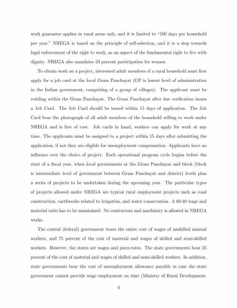
work guarantee applies in rural areas only, and it is limited to “100 days per household

per year.” NREGA is based on the principle of self-selection, and it is a step towards

legal enforcement of the right to work, as an aspect of the fundamental right to live with

dignity. NREGA also mandates 33 percent participation for women.

To obtain work on a project, interested adult members of a rural household must first

apply for a job card at the local Gram Panchayat (GP is lowest level of administration

in the Indian government, comprising of a group of villages). The applicant must be

residing within the Gram Panchayat. The Gram Panchayat after due verification issues

a Job Card. The Job Card should be issued within 15 days of application. The Job

Card bear the photograph of all adult members of the household willing to work under

NREGA and is free of cost. Job cards in hand, workers can apply for work at any

time. The applicants must be assigned to a project within 15 days after submitting the

application, if not they are eligible for unemployment compensation. Applicants have no

influence over the choice of project. Each operational program cycle begins before the

start of a fiscal year, when local governments at the Gram Panchayat and block (block

is intermediate level of government between Gram Panchayat and district) levels plan

a series of projects to be undertaken during the upcoming year. The particular types

of projects allowed under NREGA are typical rural employment projects such as road

construction, earthworks related to irrigation, and water conservation. A 60:40 wage and

material ratio has to be maintained. No contractors and machinery is allowed in NREGA

works.

The central (federal) government bears the entire cost of wages of unskilled manual

workers, and 75 percent of the cost of material and wages of skilled and semi-skilled

workers. However, the states set wages and piece-rates. The state governments bear 25

percent of the cost of material and wages of skilled and semi-skilled workers. In addition,

state governments bear the cost of unemployment allowance payable in case the state

government cannot provide wage employment on time (Ministry of Rural Development,

4

2008).

With a budget of almost 4 billion USD or 2.3 percent of total central government

spending, the program is by far the best endowed anti-poverty program in India (Ministry

of Rural Development, 2008a). During the first year of implementation (2006-07) in 200

districts, 21 million households were employed and 905 million person days of work were

generated. In 2007-08, 33.9 million households were provided employment and 1.4 billion

working days were generated in 330 districts (Ministry of Rural Development, 2010).

Given the scale, NREGA ranks among the major workfare initiatives worldwide.

NREGA has attracted a considerable amount of academic interest because of its size

and its implications for rural India. Ravi and Englar (2009) use data collected from one

district (Medhak) of Andhra Pradesh, a state in the Southern India to look at the impact

of the program on food security, savings, and health outcomes. They use a single cross

section data containing 1066 households collected in June 2007 (when NREGA was al-

ready operational in the district) to implement Propensity Score Matching (PSM). They

also use a subsequent panel data of 320 households (collected in December 2008) to im-

plement a double difference and triple difference. Since NREGA was already operational

in the district when their baseline data was collected, they use new joiners, long-term par-

ticipants, and other constructed groups to implement their double and triple difference

strategy. They find that NREGA significantly increases expenditure on food by 40 per-

cent and non food consumables by 69 percent. They also find that the program improves

the probability of holding saving by 9 percent.

Liu and Deininger (2010) use a panel data for 2500 households, collected in 2004, 2006,

and 2008, from five districts in Andhra Pradesh, a state in the Southern India to study

the impact of NREGA participation on consumption expenditure, calorie consumption,

protein intake, and asset accumulation. They employ difference-in-difference and triple

difference methodology. They find significant impact of NREGA participation on calorie

consumption, protein intake, and consumption expenditure. Importantly, they find an

5

impact on consumption which is greater than the direct cash transfer from NREGA, and

conclude that the short term effects of NREGA on participating households were positive

and greater than the program costs.

Khera and Nayak (2009) use qualitative data collected on 1060 NREGA workers from

98 NREGA worksites spread across 10 sample districts from six north Indian states to

examine the socio-economic consequences of NREGA for women workers. They report

that significant benefits have already started accruing to women through better access to

local employment, at minimum wages, with relatively decent and safe work conditions.8

Almost half of the NREGA women workers responded that had they not worked at the

NREGA worksites, they would have worked at home or remained unemployed. Pankaj

and Tankha (2010) based on their descriptive analysis of a field survey of NREGA workers

report that women as individuals have gained because of their ability to earn indepen-

dently, made possible due to the paid employment opportunity under NREGA. They use

information collected from 428 female NREGA workers from four northern states in India.

Thus considerable amount of literature exists on NREGA; however, there is no study,

to our knowledge, which looks at the impact of NREGA on the labor market outcomes.

The existing studies (for example, Khera and Nayak (2009) and Pankaj and Tankha

(2010)) are descriptive in nature, and report responses from female NREGA workers.

Ravi and Englar (2009) and Liu and Deininger (2010) try to estimate the impact of

NREGA on the ‘participants’ known as the effect of “Treatment-on-Treated” (TOT).

Besides their samples being restricted to one and five districts in the state of Andhra

Pradesh, respectively, they only concentrate on consumption outcomes (not on the labor

market outcomes).

Our paper contributes by estimating the causal impacts of NREGA on the labor

market outcomes using nationally representative data. Our data contain all districts

8Their analysis relies on percentage of female NREGA workers reporting that NREGA helped to avoidhunger, migration, illness, hazardous work etc.

6

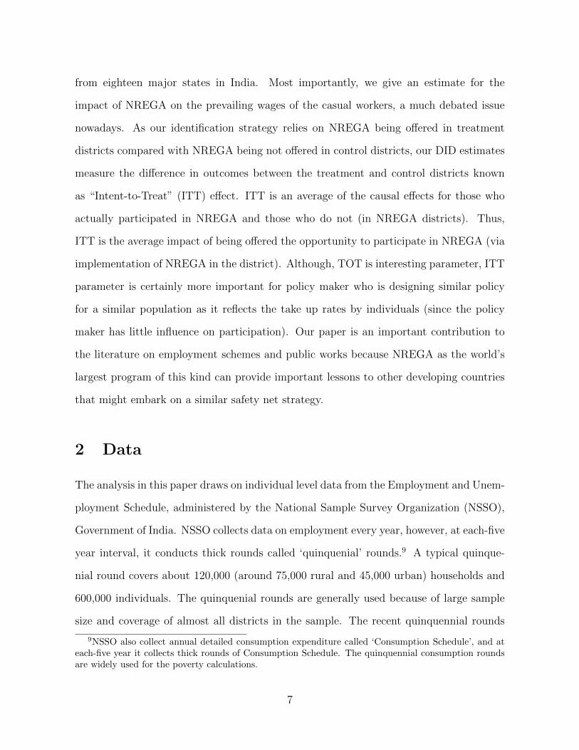
from eighteen major states in India. Most importantly, we give an estimate for the

impact of NREGA on the prevailing wages of the casual workers, a much debated issue

nowadays. As our identification strategy relies on NREGA being offered in treatment

districts compared with NREGA being not offered in control districts, our DID estimates

measure the difference in outcomes between the treatment and control districts known

as “Intent-to-Treat” (ITT) effect. ITT is an average of the causal effects for those who

actually participated in NREGA and those who do not (in NREGA districts). Thus,

ITT is the average impact of being offered the opportunity to participate in NREGA (via

implementation of NREGA in the district). Although, TOT is interesting parameter, ITT

parameter is certainly more important for policy maker who is designing similar policy

for a similar population as it reflects the take up rates by individuals (since the policy

maker has little influence on participation). Our paper is an important contribution to

the literature on employment schemes and public works because NREGA as the world’s

largest program of this kind can provide important lessons to other developing countries

that might embark on a similar safety net strategy.

2 Data

The analysis in this paper draws on individual level data from the Employment and Unem-

ployment Schedule, administered by the National Sample Survey Organization (NSSO),

Government of India. NSSO collects data on employment every year, however, at each-five

year interval, it conducts thick rounds called ‘quinquenial’ rounds.9 A typical quinque-

nial round covers about 120,000 (around 75,000 rural and 45,000 urban) households and

600,000 individuals. The quinquenial rounds are generally used because of large sample

size and coverage of almost all districts in the sample. The recent quinquennial rounds

9NSSO also collect annual detailed consumption expenditure called ‘Consumption Schedule’, and ateach-five year it collects thick rounds of Consumption Schedule. The quinquennial consumption roundsare widely used for the poverty calculations.

7

available are conducted in 1999-00, 2004-05, and 2009-10.10 As NREGA was implemented

in phases starting from February 2006, the 2004-05 (61st Round) data serve as baseline.

The “small round” surveys of the NSSO conducted annually are usually considered to

be of limited use in capturing trends, because their smaller size makes them incomparable

with the quinquennial large surveys.11 However, NSSO conducted a much larger Employ-

ment and Unemployment Round survey in 2007-08 (64th round) annual series whose main

concentration is on employment and migration. The 2007-08 data covered almost all dis-

tricts in India with a sample size of 125,578 households (79,091 rural and 46,487 urban)

and 572,254 persons. The 2007-08 survey is comparable to the usual quinquennial survey

in terms of size, questions, and coverage of all districts. It therefore allows us to examine

the impacts of NREGA using this as a post treatment (coverage) data in combination

with the 2004-05 data, which served as baseline. Since the third Phase districts remained

uncovered in 2007-08 data (as Phase III was implemented in 2008-09), it demarcates the

treated and control districts. The Phase I and Phase II districts have operationalized

NREGA, while there was no NREGA in the Phase III districts in 2007-08. We group the

Phase I and Phase II districts together and call them as ‘treatment’ districts, while we

call Phase III districts as ‘control’ districts.

NSS classifies workers into three groups: self-employed, regular salaried and casual

workers. Casual workers are daily wage workers and NREGA is targeted towards them.

Our main variables of interest are labor market outcomes such as the share of public

works in total casual workforce, and real wages of casual workers. We also look into how

NREGA has affected the labor force participation decision.12 We also use the Employment

10The year refers to July-June, i.e. July 1999-June-2000.11Also not all districts are covered.12We would have liked to look at the impact of NREGA on consumption and poverty. The Employment

Rounds also collect aggregated consumption expenditure in addition to detailed employment informa-tion. However, for consumption and poverty estimates in India, Consumption Rounds are used as theycollect very detailed information on expenditure. We do have thick round Consumer Survey in 2004-05,however, unlike the 2007-08 Employment Survey the 2007-08 annual Consumer Survey is small and isnot comparable with the thick round Consumption Survey conducted in 2004-05 in terms of sample sizeand coverage. This restricts us from implementing our empirical strategy for consumption and poverty

8

and Unemployment round for year 1999-00 to test for existing differential trends between

NREGA and non-NREGA districts when there was no NREGA in any of the districts.

The information about phase wise expansion of NREGA in different districts comes from

NREGA program webpage (http://nrega.nic.in). Nominal wages are adjusted using state

specific consumer price indexes for agriculture laborers, and weekly wages are divided by

number of days worked to get daily wages.13 We also restrict our attention to people in

age group 18-60. Details about variable construction, matching of districts across surveys

are given in the data appendix.

Table 1 presents the descriptive statistics of treatment and control districts in year

2004-05 when there was no NREGA. The Phase I and Phase II districts (treatment

districts) are indeed backward compared to the Phase III districts (control districts). The

treatment districts have a larger share of SC/ST population who are the disadvantaged

group in India. Similarly, the treatment districts’ population has comparatively worse

education distribution. In terms of labor force participation, the treatment districts have

lower (higher) labor force participation for female and SC/ST (male) compared to control

districts. However, the treatment districts have marginally higher share of public works in

the casual work. More importantly, the poverty rate is almost 12% higher in the treatment

districts compared to the control districts (32% compared with 20%). The average per

capita expenditure is also much lower in treatment districts compared with the average

per capita expenditure in the control districts. Thus the descriptive analysis suggests that

there was effective targeting of NREGA towards backward districts, in the initial phases

of NREGA.

outcomes.13NSS does not collect information on hours of work but report time intensity of work for each day in

the reference week assigning 1 day for 4 or more hours of work during a day and 0.5 day for 1-4 hours ofwork.

9

3 Empirical Methodology

3.1 Difference-in-Difference

The phase wise implementation of NREGA across Indian districts creates a ‘natural ex-

periment’ that is unique for a large program such as NREGA.14 We exploit this phase wise

expansion to implement our difference-in-difference strategy. As discussed in previous sec-

tion, we define those districts as treatment districts where NREGA was implemented in

Phase I and Phase II (in 2007-08 data, NREGA was operational in these districts), while

the control districts are those where NREGA was implemented in Phase III (2008-09)—so,

in 2007-08 data, NREGA was not operational in these control districts.

Given that the criterion on which districts were selected in different phases are not in

the public domain (except the notion of ‘backward districts’), the DID has its advantage

as it does not require us to specify the rules by which the treatment is assigned. In

addition, the treatment and comparison groups do not necessarily need to have the same

pre intervention conditions (World Bank, 2011, p99).15 To apply DID, all that is necessary

is to measure outcomes in the group that receives the program (the treatment group) and

the group that does not (the comparison group) both before and after the program.16

We use the following model to identify the impact of NREGA17

Yidt = β.D07t + τDID.Wdt + γ.Xidt + µd + εidt (1)

The dependent variable Yidt represents outcome of interest for individual i in district

14We call this a ‘natural experiment’ as the phase wise expansion is effectively used to define treatmentand control groups (Imbens and Wooldridge, 2009, p 67).

15As NREGA was not implemented randomly across districts, but more backward districts were chosenfirst, this will result in selection bias. The advantage of DID estimator is that it eliminates selection biasunder the assumption that the selection bias enters additively and does not change over time.

16The key assumption of DID is that the time trend in the absence of NREGA would have been thesame in both NREGA and non-NREGA districts.

17The specification follows closely what is suggested by the literature on use of DID method for impactevaluation. See, for example, Imbens and Wooldridge, 2009, p 67-68.

10

d at time t (t=2004-05, 2007-08).18’19 The binary variable D07t takes a value 1 for year

2007-08 and 0 for year 2004-05—D07t is the time effect common to all districts. Wdt is

equal to the interaction of the treatment group and year indicator, i.e. Wdt = Td ∗D07t,

where Td takes a value 1 if district d is in treatment group (districts where NREGA was

operational in 2007-08, i.e. Phase I and Phase II districts) and 0 otherwise (Phase III

districts which did not have operational NREGA in 2007-08). µd is a fixed effect unique

to a district. Xidt is a matrix of individual level controls such as age, square of age,

dummies for education levels, indicators for male, and SC/ST. The disturbance term εidt

summarizes the influence of all other unobserved variables that vary across individuals,

districts, and over time. In this framework, the parameter β identifies the year effect on

outcome—the effect of any systematic changes that affected all districts between 2004-

05 and 2007-08. The parameter τDID is the parameter of interest which identifies DID

estimate for the impact of NREGA on the outcome of interest.

τDID gives us the difference in outcomes between the treatment and control districts

which is known as “Intent-to-Treat” (ITT). ITT estimates the average effect of the treat-

ment on the outcome of interest of all eligible individuals, irrespective of their participation

into the program. Thus, ITT is the average impact of being offered the opportunity to

participate in NREGA (via implementation of NREGA in the district). Although, from

the perspective of NREGA literature, it is also desirable to have an estimate of the impact

of actually participating in the program (known as the effect of “Treatment-on-Treated”

(TOT)), ITT parameter is more important for policy maker who is designing similar pol-

icy for a similar population as it reflects the take up rates by individuals (since the policy

18One of the reasons for using individual level information over district level aggregates is to capture theobservable heterogeneity across individuals/households. No matter how small is the difference, it is alwaysprudent to extend the analysis beyond comparisons of means. The inclusion of individual/household levelcontrol variables accounting for the “observable” heterogeneity reduces any statistical bias associated withheterogeneity between households/individuals in treatment and control localities (Behrman and Todd,1999).

19Using individual level data increases the precision of the estimates. However, using individual leveldata with grouped data requires standard error correction (Angrist and Pischke, 2011). Since our variablesof interest are grouped over district-year, we report standard errors clustered at district-year.

11

maker has little influence on participation).20

3.2 Falsification Test

One key assumption of DID estimation is that the trends in outcomes of interest would

have been same in both the groups (NREGA and non-NREGA districts) in the absence

of NREGA, and implementation of NREGA induced a deviation from the common trend.

Although, the districts with operational NREGA and without operational NREGA can

differ, this difference is meant to be captured by district fixed effects.21 Unfortunately,

there is no way for us to prove that the differences between the treatment (NREGA dis-

tricts) and comparison (non-NREGA districts) districts would have moved in tandem in

the absence of the program. However, if the outcomes moved in tandem before the pro-

gram started, we gain confidence that outcomes would have continued to move in tandem

in the post intervention period (without the intervention). To test the assumption of par-

allel trends we perform what is known as a “falsification” test. For this test, we performed

an additional difference-in-differences estimation using a “fake” treatment. We use data

from 1999-00 and 2004-05 to estimate difference-in-difference using the same treatment

and comparison group districts. The only exception is that there was no NREGA in both

the periods in all the districts. Thus we estimate the following:

Yidt = β.D04t + τDID.Wdt + γ.Xidt + µd + εidt (2)

The binary variable D04t takes a value 1 for year 2004-05 and 0 for year 1999-00. Wdt

20One could potentially recover TOT from ITT under the assumption that operationalization ofNREGA in a district does not have affected the non-participants’ outcomes in the NREGA districts.However, we believe that this assumption is not valid in our case as operationalization of NREGA ina district probably will have an effect on the outcomes of non-participants residing in the treatmentdistrict. For example, there may be an upward pressure on the wages of non-participants daily wageworkers because of the increased demand for daily wage workers after operationalization of NREGA.

21One of the criticism of DID is that although DID captures the time invariant factors well, it fail totake account of time varying factors. However, we believe that we believe that controlling for individualcharacteristics take account of most of the time varying factors.

12

is equal to the interaction of the treatment group and year indicator, i.e. Wdt = Td ∗D04t.

If the outcomes were moving in tandem, then we should expect the ‘fake DID (i.e. τDID)’

estimates to be not different from zero.

3.3 Allowing for differential effects of NREGA

As 2007-08 was the second year of NREGA in Phase I districts, while it was the first year

of NREGA in the Phase II districts, we use Phase I and Phase II districts as two separate

treatment groups to capture the differential effects of NREGA on these two groups. The

control group remains the Phase III districts, where there was no NREGA in 2007-08.

We use the following model to identify differential impacts of NREGA on Phase I and

Phase II districts:

Yidt = β.D07t + τDID1.(Phase1 ∗D07t) + τDID2.(Phase2 ∗D07t) + γ.Xidt + µd + εidt (3)

where Phase1 takes a value 1 if the districts were covered in the Phase I (2006-07) and 0

otherwise. Similarly, Phase2 takes a value 1 if the districts were covered in the Phase II

(2007-08) and 0 otherwise. Our interest parameters τDID1 and τDID2 capture the impact

of NREGA in Phase I and Phase II districts, respectively. We also test for the equality

of NREGA’s impacts across Phase I and Phase II districts, i.e. τDID1 = τDID2.

4 Results

Our first and second sets of results present the impact of NREGA on employment in

public works programs and labor force participation, respectively. The third set of results

presents impact of NREGA on real wages of casual workers.

13

4.1 Employment in public works

Did NREGA increase participation in public works? Ex-ante one would believe that as

NREGA provide more public works opportunities, operationalization of NREGA will in-

crease the participation of casual workers in public works. However, without comparing

NREGA districts with non-NREGA districts, it is difficult to establish whether the in-

crease in public works share is because of NREGA. For example, it is also possible that

overall ongoing development in rural areas (for example, road construction to increase the

accessibility of rural areas) might also increase the public works opportunities in districts

which did not have operational NREGA in 2007-08. Given that the non-NREGA districts

were better off to start with, it might be plausible that increase in the public work oppor-

tunities in these districts might not be less than the increase in public work opportunities

in NREGA districts. Before proceeding to estimate the impacts of NREGA on other labor

market outcomes, it is essential to establish that NREGA led to a significant increase in

public works opportunities in the NREGA districts compared with non-NREGA districts.

Only 0.8 percent of the casual workers in NREGA districts reported working in public

works in 2004-05, while this share was 0.6 percent in non-NREGA districts (Table 1).22

Panel I of Table 2 reports the results of our DID estimates. Overall, there has been

an increase in the probability of a casual worker to be engaged in public works across

all districts between 2004-05 and 2007-08 (captured by the time effect). However, this

increase in probability is much larger in NREGA districts compared with non-NREGA

districts. Our DID estimates show that the probability of a casual worker being engaged

in public works increased by 2.5 percentage points more in NREGA districts compared

to non-NREGA districts. We find similar results for male, female, and SC/ST workers.

Importantly, there has been no significant increase in the probability of a female casual

worker being engaged in public works between 2004-05 and 2007-08 in the non-NREGA

22This is an annual average implying that throughout the year, 0.8 (0.6) percent of casual workers areemployed in public works in NREGA (non-NREGA) districts.

14

districts. However, the probability of a female casual worker being engaged in the public

works increased by 4 percentage points more in NREGA districts compared to the non-

NREGA districts between 2004-05 and 2007-08. Hence, our DID estimates establish that

NREGA has led to a significant increase in public works participation in NREGA districts.

Next, we check whether our DID estimates are confounded by differential pre-program

trends between NREGA and non-NREGA districts. Panel II of Table 2 presents the results

of the falsification exercise where we estimate a ‘fake DID’ using 1999-00 and 2004-05 data,

when there was no program in both the periods. We do not find any evidence of differential

pre-program trend in the probability of a casual labor participating in the public works.

Indeed, there was almost no increase in probability of participation by casual worker in

public works between 1999-00 and 2004-05, and there was no difference in trends between

NREGA and non-NREGA districts. The results of the falsification exercise increase our

confidence in the DID estimates and we conclude that public works participation increased

significantly in NREGA districts because of the NREGA program.

4.2 Labor force participation

The next question we answer is whether NREGA led to an increase in labor force par-

ticipation? But before proceeding further, it is important to address why one should

expect an impact on labor force participation decision because of NREGA. We expect an

impact of NREGA on labor participation especially female labor participation because

of following reasons. First, as NREGA is rights based program, people who were not in

the labor force might be induced to get into labor force knowing that they will get work.

Second, there are many positive incentives inbuilt in NREGA for female workers. For

example, the wages paid in NREGA works are equal across gender. The female workers

are paid much less in non-public works than their male counterparts, and the statutory

minimum wages (see appendix Table A1). A higher wage offered in NREGA works com-

15

pared to prevailing wages adds additional incentive for female workers to work. Similarly,

the Act stipulates that work be provided locally, within five kilometers of the residence.

This makes participation in NREGA work feasible for women as they continue to bear

the main responsibility of household work (Khera and Nayak, 2009). Another incentive

for women workers is that each NREGA work site has to ensure that proper childcare is

provided.23 Thus, ex-ante, we believe that the operationalization of NREGA should have

a positive impact on the labor force participation decision, especially for women workers.

Khera and Nayak (2009) report that many of the female respondents at NREGA worksites

reported that the NREGA opened up a new opportunity for them.

Our DID estimates (reported in Panel I of Table 3) suggest that NREGA has a positive

impact on overall labor participation. The positive impact is more pronounced in the case

of female labor participation. The overall time effect has a negative coefficient, which

suggest that the overall labor force participation declined between 2004-05 and 2007-

08 in non-NREGA districts; however, because of the positive impact of NREGA, the

fall in labor participation (especially female participation) is lower in NREGA districts

compared with the non-NREGA districts. Other studies that have compared the 2004-

05 ‘quinquennial round’ data with the 2009-10 ‘quinquennial round’ data also document

the decline in labor force participation during this period (Chowdhury, 2011). There are

many reasons put forward for a declining trend in labor force particpation between 2004-

05 and 2009-10 such as reduction in subsidiary employment, increase in level of income

in rural areas due to increase in real wages, higher level of participation in education, etc

(Government of India, 2011).24 Without going further into the discussion on decline in

23If more than five children below the age of six years are present at the worksite, a person (preferablya woman) should be engaged under NREGA work to look after them. She will be paid a wage equal tothe prevalent wage rate paid to the unskilled worker (Ministry of Rural Development, 2008b).

24The proportion of female in age group 18-60 who reported attending school went up marginallybetween 2004-05 and 2007-08 from 1.6 (2.2) to 1.8 (2.8) in NREGA (non-NREGA) districts. Simi-larly, proportion of 18-60 aged men attending school increased from 3.7 (4.2) to 3.9 (5.3) in NREGA(non-NREGA) districts. Thus increased participation in schooling does not entirely explain the declineobserved in labor force participation.

16

labor force participation as it deserves a separate investigation, we conclude that positive

impact of NREGA is felt as the decline in labor force participation in NREGA districts

has been less than the decline in labor force participation in the non-NREGA districts.

If the long run trends in labor force participation differ between NREGA and non-

NREGA districts, then we risk interpreting pre-existing differences in labor force partic-

ipation as treatment effect (impact of NREGA). Hence, we performed the falsification

exercise whose results are given in Panel II of Table 3. We fail to reject the null of the

‘fake DID’ being zero for overall, male and female. This suggests that the labor force

participation for overall, male and female were moving in tandem before the implementa-

tion of NREGA. For the SC/ST we reject that the ‘fake DID’ is zero. Hence, we cannot

conclude convincingly for SC/ST as the DID estimate for SC/ST is also not significant.

4.3 Impact on wage rates of casual workers

It is well known that women’s involvement in NREGA has been much larger than what

was mandated by the Act.25 There is no wage differential across gender in NREGA

works. This is in contrast to non-public works in rural areas, where a large wage gap is

observed across genders. Further, average wages received by female workers in NREGA

are significantly higher than those received in other types of casual work. As discussed in

the previous sections, female participation in public works increased. This will push up

the average wages for female; however, there might be indirect effects also. For example,

other types of casual work which pay much less to female workers may be forced to offer

higher wages as a result of competition generated by NREGA. This suggests that because

of NREGA one should see at least an increase in real wages for female casual workers and

reduction in gender gap in wages.

The DID estimates (reported in Panel I of Table 4) suggest that for both male and

25The Act mandates at least one-third female beneficiaries among the total NREGA beneficiaries.

17

female workers in rural areas, NREGA has made a difference in terms of increases in the

wages of casual workers. Overall, casual workers in NREGA districts have experienced a 5

percent more increase in real wages compared to casual workers in non-NREGA districts:

the effect of NREGA is more pronounced for female workers compared to male workers

(8.3 percent compared to 3.8 percent). Similarly, SC/ST casual workers also experienced a

larger increase in wages in NREGA districts compared to SC/ST workers in non-NREGA

districts.

We run the falsification exercise to check how much our DID results are confounded by

difference in long term trends in real wages between NREGA and non-NREGA districts.

The results of falsification exercise are presented in Panel II of Table 4. In the falsification

exercise, we fail to reject that the ‘fake DID’ estimates are different from zero in the case

of overall, male, and female wages. However, we find a significant pre program difference

in trends between NREGA and non-NREGA districts in the case of SC/ST workers. This

casts doubt over our DID estimates for SC/ST workers. Similarly, although the ‘fake

DID’ estimate in falsification exercise for male workers is insignificant, it has a positive

coefficient (0.031) which in turn suggest that our DID estimate for male workers (0.038)

is overestimating the effect of NREGA on male wages. What remains certain is that

NREGA has a significant and positive impact on the female wages as it seems to be

not confounded by the pre program differential trends in wages between NREGA and

non-NREGA districts. Real wages of female casual workers increased about 8% more

in NREGA districts compared to non-NREGA districts, and this increase in female real

wages pushed up the overall average real wages in the NREGA districts more than the

increase experienced in the non-NREGA districts. The real wages increased in non-

NREGA districts also (captured by the time effect in Panel I of Table 3). Thus NREGA

has been successful in raising the female wages more than the male wages and thus

reducing the existing gender wage gap in casual works.

18

4.4 Differential effects of NREGA

Did duration of the program exposure matter? In 2007-08, Phase II districts were exposed

to NREGA for the first year, while it was second year of the program in Phase I districts.

Table 5 reports the results of the model (Equation 3) which allows NREGA impacts

to differ across Phase I and Phase II districts. Part A of Table 5 reports the results for

public works participation among casual workers. The DID estimates suggest the impacts

of NREGA on the public works participation have been larger in the Phase II districts.

However, we could not reject the null of equal effect of NREGA in Phase I and Phase II

districts based on F -test.

Part B of Table 5 presents the results for labor force participation. Here also, the

DID estimates suggest NREGA’s impacts have been larger in Phase II districts, however,

we could not reject the null of equal impacts in Phase I and Phase II districts based on

F -test. Part C of Table 5 presents the results of NREGA’s impacts on wages. Again, we

could not reject the null that the impacts have been similar in both phases. Thus the

results of Table 5 show no robust evidence of differential effects of NREGA across Phase

I and Phase II districts.

5 Conclusion

The National Rural Employment Guarantee Act (NREGA) of India is the largest employ-

ment guarantee program in the World with an annual central budget of 8.92 billion USD

in 2010-11. The Act was passed in August, 2005 and entitles every rural household in

India to a minimum of 100 days of paid work. The Act was implemented in three phases

across rural India. Using nationally representative National Sample Surveys (NSS), we

exploit the phase wise expansion of NREGA in difference-in-difference (DID) framework

to estimate casual impacts (“Intent-to-Treat”) of NREGA on the participation in public

19

works, labor force participation, and average wages of casual workers. Using two rounds

of pre-program data, we also demonstrate that our main conclusions based on the DID

estimates are not confounded by the pre-program differential trends between NREGA and

non-NREGA districts.

We find a significant increase in public works participation as a result of NREGA.

We also find a positive impact of NREGA on labor force participation, especially female

labor force participation. Post 2004-05, there has been a negative trend in labor force

participation in rural India especially in the female labor force participation. NREGA

has helped to mitigate the worsening situation and as a result, the decline in labor force

participation in NREGA districts has been less than the decline observed in the non-

NREGA districts. We also find that NREGA has a positive impact on the wages of

female casual workers: wages of female casual workers increased by 8% more in NREGA

districts compared to non-NREGA districts. In contrast, we find only marginal positive

impact of NREGA on the wages of male casual workers. Thus NREGA has helped in

reducing the gender differential in wages for casual works by pushing up the female wages.

NREGA has improved the situation of women workers by providing higher wages and more

opportunities. This positive impact may well have longer term beneficial effects on social

and economic dynamics in rural India.

20

References

[1] Abadie, A. (2005). “Semiparametric Difference-in-Differences Estimators,” The Re-

view of Economic Studies, 72(1), 1-19.

[2] Angrist, J.D. and Pischke, J.S. (2009), “Mostly Harmless Econometrics,” Priceton

University Press.

[3] Basu, A. K., Chau, N. H., and Kanbur, R (2009), “A Theory of Employment Guar-

antees: Contestability, credibility and Distributional Concerns,” Journal of Public

Economics, 9(3-4), 482-497.

[4] Behrman, J. and Todd, P. (1999), “Randomness in the Experimental Samples of

PROGRESA –Education, Health, and Nutrition Program,” International Food Pol-

icy Research Institute, Washington, DC.

[5] Bell, B., Blundell, R., and Reenen J. V. (1999), “Getting the Unemployed Back to

Work: The Role of Targeted Wage Subsidies’”’ International Tax and Public Finance,

6(3), 339-360.

[6] Bertrand, M., Duflo, E., and Mullainathan, S. (2004), “How Much Should We Trust

Difference-in-Difference Estimators,” The Quarterly Journal of Economics, 119(1),

249-275.

[7] Besley, T. and Case, A. (2009), “Unnatural Experiments? Estimating the Incidence

of Endogenous Policies,” The Economic Journal, 110, F672-F694.

[8] Besley, T. and Burgess, R. (2004), “Can Labor Regulation Hinder Economic Perfor-

mance? Evidence from India,” The Quarterly Journal of Economics, 119(1), 91-134.

[9] Bhatia, B. and Dreze, J. (2006), “Employment Guarantee in Jharkhand: Ground

Realities,” Economic and Political Weekly, , 41(29), 3198-3202.

21

[10] Chandrasekhar, C.P. and Ghosh, J. (2011), “Public Works and Wages in Rural In-

dia,” Macro Scan.

[11] Chowdhury, S. (2011), “Employment in India: What Does the Latest Data Show?,”

Economic and Political Weekly, 46(32), 23-26.

[12] Cutler, D., Fung, W., Kremer, M., Singhal, M., and Vogl Tom. (2010), “Early-

life Malaria Exposure and Adult Outcomes: Evidence from Malaria Eradication in

India,” American Economic Journal: Applied Economics, 2(2), 72-94.

[13] Devereux, S. and Solomon, C. (2006), “Employment Creation Programmes: The

International Experience,” ILO Issues in Employment and Poverty Discussion Paper

No. 24.

[14] Datt, G. and Ravallion, M. (1994), “Transfer Benefits from Public-Works Employ-

ment: Evidence for Rural India,”’ Economic Journal, 104(427), 1346-69.

[15] Duflo, E., Glennerster, R., and Kremer, M. (2008), “ Using Randomization in De-

velopment Economics Research: A Toolkit,” In: Schultz, T. and Strauss, J (Eds.),

Handbook of Development Economics, Chapter 61, vol 4, 3895-3962.

[16] Eissa, N. and Liebman, J. (1996), “Labor Supply Response to the Earned Income

Tax Credit,” The Quarterly Journal of Economics, 111(2), 605-637.

[17] Gaiha, R. (1997), “Do Rural Public Works Influence Agricultural Wages? The Case

of the Employment Guarantee Scheme in India,”’ Oxford Development Studies, 25(3),

301-314.

[18] Galiani, S. and Gertler, P. (2005), “Water for Life: The Impact of the Privatization

of Water Services on Child Mortality,” Journal of Political Economy, 113(1), 83-120.

[19] Government of India. (2011), “Decline in Labour Force,” Press Information Bureau,

http://labour.nic.in/pib/PressRelease/DeclineLabourForce.pdf.

22

[20] Heckman, J., La Londe, R., Smith, J. (1999), ”The Economics and Econometrics of

Active Labor Market Programs,” In: Ashenfelter, A., Card, D. (Eds.), Handbook of

Labor Economics, vol. 3. Elsevier Science, Amsterdam.

[21] Hoddinott, J. and Skoufias, E. (2004), “The Impact of PROGRESA on Food Con-

sumption,” Economic Development and Cultural Change, 53(1), 37-61.

[22] Imbens, G.W. and Wooldridge, J.M. (2009), “Recent Developments in the Econo-

metrics of Program Evaluation,” Journal of Economic Literature, 47(1), 5-86.

[23] Jalan, J. and Ravallion, M. (1998), “Are there dynamic gains from a poor-area de-

velopment program?,” Journal of Public Economics, 67(1), 65-85.

[24] Katz, L.F., Kling, J.R., and Liebman, J.B. (2001), “Moving To Opportunity in

Boston: Early Results of a Randomized Mobility Experiment,” The Quarterly Jour-

nal of Economics, 116 (2), 607-654. doi: 10.1162/003355

[25] Khera, R. and Nayak, N. (2009), “Women workers and perceptions of the National

Rural Employment Guarantee Act,” Economic and Political Weekly, 44(43), 49-57.

[26] Liu, Y. and Deininger, K. (2011), “Poverty Impacts of India’s National Rural Guar-

antee Scheme: Evidence from Andhra Pradesh,” Unpublished manuscript, Paper pre-

sented at Agriculture and Applied Economics Association Annual Meeting.

[27] Meyer, B.D. (1995), “Natural and Quasi-Experiments in Economics,” Journal of

Business & Economic Statistics, 13(2), 151-161.

[28] Ministry of Rural Development. (2010), “Annual Report (2009-2010),” Government

of India.

[29] Ministry of Rural Development. (2008a), “Annual Report (2007-2008),” Government

of India.

23

[30] Ministry of Rural Development. (2008b), “The National Rural Employment Guar-

antee Act 2005 (NREGA): Operational Guidelines 2008,” Government of India.

[31] National Sample Survey Organization. (2010), “Employment and Unemployment

Situation in India 2007-08,” Report No. 531 (64/10.2/1), Government of India.


Situation in India 2004-05,” Report No. 515(61/10/1), Government of India.


Situation in India 1999-00,” Report No. 458(55/10/2), Government of India.

[34] Ninno, C.D., Subbarao, K. and Milazzo, A. (2009), “How to Make Public Works

Work: A Review of the Experiences,” SP Discussion Paper, 0905, The World Bank.

[35] Pankaj, A. and Tankha, R. (2010), “Empowerment effects of the NREGA on Women

Workers: A study in four states,” Economic and Political Weekly, 45(30), 45-55.

[36] Ravallion, M. (2008), “Evaluating Anti-Poverty Programs,” In: Schultz, T. and

Strauss, J (Eds.), Handbook of Development Economics, Chapter 59, vol 4, 3787-

3846.

[37] Ravi, S. and Engler, M. (2010), “Workfare in Low Income Countries: An effec-

tive way to fight poverty? Case of India’s NREGA,” Unpublished manuscript,

http://ssrn.com/abstract=1336837.

[38] Staubli, S. (2011), “The Impact of Stricter Criteria for Disability Insurance on Labor

Force Participation,” Journal of Public Economics, 95, 1223-35.

[39] Todd, P. (2008), “Evaluating Social Programs with Endogenous Program Placement

and Selection of the Treated,” In: Schultz, T. and Strauss, J (Eds.), Handbook of

Development Economics, Chapter 60, vol 4, 3847-3894.

24

[40] World Bank (2011), “Impact Evaluation in Practice,” Washington DC.

[41] World Bank (2011), “Social Protection for a Changing India,” Washington DC.

25

Data Appendix

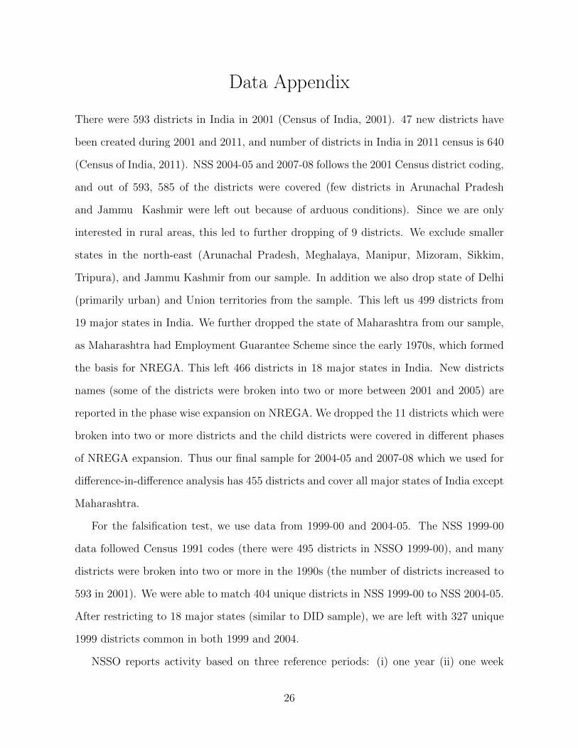
There were 593 districts in India in 2001 (Census of India, 2001). 47 new districts have

been created during 2001 and 2011, and number of districts in India in 2011 census is 640

(Census of India, 2011). NSS 2004-05 and 2007-08 follows the 2001 Census district coding,

and out of 593, 585 of the districts were covered (few districts in Arunachal Pradesh

and Jammu Kashmir were left out because of arduous conditions). Since we are only

interested in rural areas, this led to further dropping of 9 districts. We exclude smaller

states in the north-east (Arunachal Pradesh, Meghalaya, Manipur, Mizoram, Sikkim,

Tripura), and Jammu Kashmir from our sample. In addition we also drop state of Delhi

(primarily urban) and Union territories from the sample. This left us 499 districts from

19 major states in India. We further dropped the state of Maharashtra from our sample,

as Maharashtra had Employment Guarantee Scheme since the early 1970s, which formed

the basis for NREGA. This left 466 districts in 18 major states in India. New districts

names (some of the districts were broken into two or more between 2001 and 2005) are

reported in the phase wise expansion on NREGA. We dropped the 11 districts which were

broken into two or more districts and the child districts were covered in different phases

of NREGA expansion. Thus our final sample for 2004-05 and 2007-08 which we used for

difference-in-difference analysis has 455 districts and cover all major states of India except

Maharashtra.

For the falsification test, we use data from 1999-00 and 2004-05. The NSS 1999-00

data followed Census 1991 codes (there were 495 districts in NSSO 1999-00), and many

districts were broken into two or more in the 1990s (the number of districts increased to

593 in 2001). We were able to match 404 unique districts in NSS 1999-00 to NSS 2004-05.

After restricting to 18 major states (similar to DID sample), we are left with 327 unique

1999 districts common in both 1999 and 2004.

NSSO reports activity based on three reference periods: (i) one year (ii) one week

26

and (iii) each day of the reference week. Based on these three reference periods, three

different measures of activity status are reported as usual status, current weekly status

and current daily status. The convention in most developing countries in the world is to

measure labor force related variables on the basis of weekly status. Hence, we choose to

use the current weekly status. The current weekly status has two broad advantages over

usual status. First, it is more likely to capture the participation in public works. Second,

the wages reported are the wages earned during the last week, thus current weekly status

provide a direct link to type of work and wages earned.

27

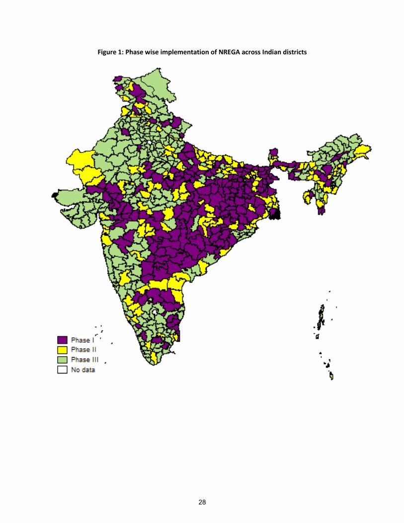
Figure 1: Phase wise implementation of NREGA across Indian districts

28

Table-1: Descriptive statistics of NREGA and non-NREGA Districts, 2004-05

Treatment

Group Control Group Difference

Phase I districts

Phase II districts

NREGA Phase I & II

districts

NREGA Phase III districts (T-C)

Percentage of Phase I Phase II SCs/STs 35.1 30.4 33.26 26.67

6.59

Male 50.9 50.7 50.85 50.96

-0.12

Average age 25.3 25.7 25.49 26.43

-0.94

Below primary 70.1 67.5 69.07 60.17

8.90

Primary 12.1 13.1 12.50 14.81

-2.31

Middle 9.5 10.0 9.72 13.20

-3.48

Secondary 4.4 5.1 4.69 6.28

-1.60

Higher Secondary 2.2 2.5 2.32 3.05

-0.73

Tertiary 1.6 1.8 1.71 2.49

-0.78

LFPR (18-60) 69.2 65.2 67.67 70.44

-2.77

Male 93.2 93.1 93.16 92.39

0.77

Female 45.8 38.5 42.92 48.48

-5.56

SC/ST 73.9 68.7 72.00 73.64

-1.64

Public work in casual labor (18-60) 0.7 0.9 0.79 0.62

0.17

Male 0.6 0.7 0.64 0.47

0.17

Female 0.9 1.4 1.10 0.95

0.15

SC/ST 1.0 0.8 0.98 0.71

0.27

Work Force participation (18-60) 67.1 62.8 65.42 67.48

-2.07

Unemployment (18-60) 1.8 2.2 1.94 2.47

-0.53 Average daily wage in casual work (18-60) 44.7 48.6 59.34 76.29

-16.95

Male 49.8 53.8 67.53 86.22

-18.69

Female 33.4 36.8 39.43 49.78

-10.35

SC/ST 43.4 48.0 51.24 65.59

-14.35

Poverty Rate† 35.9 26.1 32.08 20.71

11.37

Per capita expenditure (in INR at 2004-05 prices)† 483.3 539.3 505.02 646.00 -140.98

Notes: † Calculated from NSS 61

st (2004-05) consumption round survey.

29

Table-2: Impact of NREGA on public work participation

Dependent Variable: Works in public work=1; Work as casual labor but not in public works=0

Panel I: DID Estimates Panel II: Falsification Test

All Male Female SCs/STs All Male Female SCs/STs

Year1=2007-08 ; Year0=2004-05 Year1=2004-05 ; Year0=1999-00

Dummy for Year 1 (Base year 0) 0.007*** 0.007*** 0.002 0.008*** -0.001 -0.003 0.002 0.001

(0.002) (0.002) (0.002) (0.003) (0.003) (0.003) (0.005) (0.004) NREGS districts* Dummy for year 1

0.025*** 0.020*** 0.038*** 0.022*** -0.001 -0.002 -0.002 -0.002

(0.006) (0.005) (0.009) (0.006) (0.004) (0.004) (0.006) (0.006)

District Fixed effects Yes Yes Yes Yes Yes Yes Yes Yes

Observations 52,353 37,002 15,351 24,726 43,706 30,519 13,187 20,430

R-squared 0.132 0.112 0.276 0.140 0.132 0.109 0.277 0.143

Note: Robust standard-errors are in parenthesis clustered at district-year level. The model also include individual level characteristics

such as age, square of age, dummies for education levels (primary, middle, secondary, senior secondary, and tertiary), male, and

SC/ST.

*** Significant at 1 percent level. **Significant at 5 percent level. *Significant at 10 percent level.

30

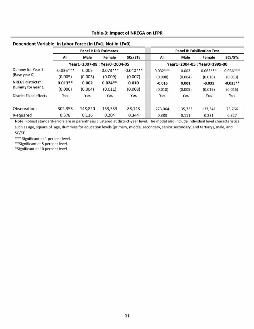
Table-3: Impact of NREGA on LFPR

Dependent Variable: In Labor Force (In LF=1; Not in LF=0)




Dummy for Year 1 (Base year 0)

-0.036*** 0.005 -0.073*** -0.040*** 0.032*** 0.003 0.063*** 0.036***


0.013** 0.002 0.024** 0.010 -0.015 0.001 -0.031 -0.035**

(0.006) (0.004) (0.011) (0.008) (0.010) (0.005) (0.019) (0.015)


Observations 302,353 148,820 153,533 88,143 273,064 135,723 137,341 75,766

R-squared 0.378 0.136 0.204 0.344 0.383 0.111 0.231 0.327



SC/ST.


31

Table-4: Impact of NREGA on real wages of casual labor

Dependent Variable: log of real wage





0.108*** 0.091*** 0.149*** 0.105*** 0.075*** 0.084*** 0.052* 0.045**


0.049*** 0.038** 0.083*** 0.042** 0.019 0.031 0.008 0.051*

(0.017) (0.017) (0.026) (0.020) (0.023) (0.023) (0.033) (0.027)


Observations 50,188 35,784 14,404 23,720 41,179 29,024 12,155 19,259

R-squared 0.476 0.464 0.359 0.467 0.484 0.458 0.412 0.471



SC/ST.


32

Table-5: Differential impacts of NREGA Panel I: DID Estimates Panel II: Falsification Test

All Male Female SCs/STs

All Male Female SCs/STs

Year1=2007-08 ; Year0=2004-05

Year1=2004-05 ; Year0=1999-00

Part A: Public worker in casual work

Dependent Variable: In public work conditional on being casual labor (Works in public work=1; Work as casual labor but not in public works=0) Dummy for Year 1 (Base year 0)

0.007*** 0.007*** 0.002 0.008***

-0.001 -0.003 0.002 0.001

(0.002) (0.002) (0.002) (0.003)

(0.003) (0.003) (0.005) (0.004) Phase I districts* Dummy for year 1

0.018*** 0.016*** 0.027*** 0.019***

-0.004 -0.004 -0.003 -0.006

(0.005) (0.004) (0.006) (0.007)

(0.006) (0.005) (0.008) (0.008) Phase II districts* Dummy for year 1

0.036*** 0.027*** 0.058*** 0.028***

0.003 0.003 -0.000 0.005

(0.012) (0.009) (0.020) (0.010)

(0.004) (0.004) (0.005) (0.007)

F-test: Equal Treatment Effects (p-values)

0.172 0.288 0.134 0.460

0.215 0.198 0.681 0.253

Observations 52,353 37,002 15,351 24,726 43,706 30,519 13,187 20,430 R-squared 0.133 0.112 0.277 0.140 0.132 0.109 0.277 0.143

Part B: Labor force participation

Dependent Variable: In Labor Force (In LF=1; Not in LF=0)


-0.036*** 0.005 -0.073*** -0.040***

0.032*** 0.003 0.063*** 0.036***

(0.005) (0.003) (0.009) (0.007)


0.010 0.002 0.019 0.005

-0.020* 0.001 -0.043** -0.039**

(0.007) (0.004) (0.013) (0.009)


0.017** 0.003 0.031** 0.019**

-0.006 0.001 -0.013 -0.028*

(0.007) (0.005) (0.013) (0.009)

(0.012) (0.006) (0.022) (0.017)


0.287 0.844 0.302 0.102

0.212 0.986 0.158 0.460


Part C: Real wages of casual labor

Dependent Variable: log of real wage Dummy for Year 1 (Base

year 0) 0.108*** 0.091*** 0.149*** 0.105***

0.075*** 0.084*** 0.052* 0.045**

(0.012) (0.012) (0.016) (0.015)


0.062*** 0.049** 0.095*** 0.069***

0.031 0.047* 0.019 0.053*

(0.020) (0.019) (0.030) (0.021)


0.029 0.021 0.064* -0.007

-0.001 0.004 -0.012 0.047

(0.024) (0.022) (0.037) (0.027)

(0.027) (0.026) (0.041) (0.035)


0.227 0.246 0.467 0.006

0.210 0.109 0.396 0.868


Note: Robust standard-errors are in parenthesis clustered at district-year level. See notes of Table 4.

33

Appendix

Table A1: Daily wage rates

States/District

Prevailing Wage Rate under NREGA

(Rs./Day) (2007-08)

Minimum Wages (2008-

09)

Prevailing Average Wage Rate (Rs./Day) for casual worker

(2007-08)

Male Female All

Assam 80 76

74 58 70

Andhra Pradesh 80 80

81 55 69

Bihar 81 81

60 51 58

Gujarat 100 100

67 58 64

Haryana 141 135

103 82 100

Himachal Pradesh 100 100

112 88 110

Karnataka 82 82

69 45 59

Kerala 125 125

171 91 154

Madhya Pradesh 91 88

54 44 50

Orissa 70 70

56 41 51

Punjab** 99 99

100 76 97

Rajasthan 100 100

85 71 82

Tamil Nadu 80 80

101 51 80

Uttar Pradesh 100 100

73 59 71

West Bengal 75 75

68 55 66

Chhattisgarh 72 72

50 42 47

Jharkhand 86 86

68 58 66

Uttaranchal 73 73 98 72 94

Source: Prevailing wages under NREGA and minimum wages are taken from Indiastat.com. Average wage of casual workers are calculated from NSS 64

th Round (2007-08) Employment and Unemployment

Round. ** Refer to Hoshiarpur region of Punjab.

34

the impact of indian job guarantee scheme on labor market ...ftp.iza.org/dp6548.pdf · unemployment...

Documents