the impact of increasing search frictions on online ... files/19-080_aae30b91-4631-422c-b843... ·...
TRANSCRIPT
The Impact of Increasing Search Frictions on Online Shopping Behavior: Evidence from a Field Experiment
Donald Ngwe Thales Teixeira
Kris Ferreira
Working Paper 19-080
Working Paper 19-080
Copyright © 2019 by Donald Ngwe, Kris Ferreira, and Thales Teixeira
Working papers are in draft form. This working paper is distributed for purposes of comment and discussion only. It may not be reproduced without permission of the copyright holder. Copies of working papers are available from the author.
The Impact of Increasing Search Frictions on Online Shopping Behavior: Evidence from a Field Experiment
Donald Ngwe Harvard Business School
Kris Ferreira Harvard Business School
Thales Teixeira Harvard Business School
The impact of increasing search frictions on online shopping behavior:
Evidence from a field experiment
Donald Ngwe
Assistant Professor
Harvard Business School
Morgan Hall 179
Boston, MA 02163
(617) 496-6585
Kris Ferreira
Assistant Professor
Harvard Business School
Morgan Hall 413
Boston, MA 02163
(617) 495-3316
Thales Teixeira
Lumry Family Associate Professor
Harvard Business School
Morgan Hall T13
Boston, MA 02163
(617) 495-6125
2
The impact of increasing search frictions on online shopping behavior:
Evidence from a field experiment
Abstract
Many online stores are designed such that shoppers can easily access any available
discounted products. We propose that deliberately increasing search frictions by placing
small obstacles to locating discounted items can improve online retailers’ margins and
even increase conversion. We demonstrate using a simple theoretical framework that
inducing consumers to inspect higher-priced items first may simultaneously increase the
average price of items sold and the overall expected purchase probability by inducing
consumers to search more products. We test and confirm these predictions in a series of
field experiments conducted with a dominant online fashion and apparel retailer.
Furthermore, using information in historical transaction data about each consumer, we
demonstrate that price-sensitive shoppers are more likely to incur search costs to locate
discounted items. Our results show that increasing search frictions can be used as a self-
selecting price discrimination tool to match high discounts with price-sensitive
consumers and full-priced offerings with price-insensitive consumers.
Keywords: e-commerce, online retailing, friction, effort, search costs, price discrimination
3
Online retail accounts for a rapidly growing proportion of revenues in many product categories.
As of the fourth quarter of 2018, e-commerce accounted for 9.8% of total U.S. retail sales,
compared to less than 4% in 2008 (U.S. Census Bureau 2018). While online retail broadens
firms’ access to consumers through an additional channel, operating margins are often lower in
online stores than in physical stores. Amazon, the largest online retailer in the U.S., averaged
1.3% in operating margins from 2011 to 2013 while its brick-and-mortar counterparts typically
experienced 6% to 10% (Rigby 2014). Reasons for this difference are well recognized: prices are
easy to compare online, discount coupons and codes have high uptake, and sellers often bear the
cost of shipping products to buyers.
These factors are in part a consequence of many online sellers’ efforts to make online
shopping as convenient as possible. Pure online sellers such as Bonobos, Wayfair, and Overstock
are known for minimizing the search, transaction, and delivery costs for shoppers in an attempt
to lure them from offline channels. In industries ranging from consumer electronics to flight and
hotel booking, third-party sites reduce search costs even further by enabling cross-website
comparisons. Dominant online sellers, such as Amazon and Alibaba, are also known for their
efforts to minimize frictions for consumers. The focus of this paper is on such firms, which have
no competitors of the same size.
This trend is in stark contrast with the practice of brick-and-mortar retailers, who have
long embraced the deliberate use of search frictions to improve in-store margin performance. In
making lower-priced and lower-margin items harder to locate, by placing the sale section in the
back of the store, using bargain bins and discount racks, or having a separate outlet store miles
away, physical stores induce a self-selection among consumers who are heterogeneous in their
willingness to pay (e.g., Coughlan & Soberman 2005; Ngwe 2017).
4
In this paper, we seek to challenge the prevailing assumption that minimizing search
frictions, i.e., facilitating consumer search across a retailer’s entire assortment, is always the
optimal strategy for dominant online retailers (Bakos 1997; Brynjolfsson & Smith 2000). We
contend that just as in physical selling contexts, careful incorporation of search frictions can
facilitate price discrimination in online retail. While the price obfuscation literature (e.g., Ellison
& Ellison 2009; Brown, Hossain & Morgan 2010) has identified ways in which firms mask
prices and thus increase search frictions through product line design and price partitioning, in our
setting we hold both constant and only vary website navigation elements.
The existing literature has typically conceived of search costs as the time, mental or
physical effort, and money required to physically identify and consider additional options prior
to making a purchase decision (Bell, Ho & Tang 1998). In offline retail contexts, these often take
the form of travel costs or time spent shopping in measurable intervals. In an interesting example
of this, Hui et al. (2013) find that increasing in-store travel as a result of changing the location of
particular products increases purchases by seven percent for a grocery store. Given the ease and
immediacy of online shopping, it is perhaps unsurprising that equivalent search costs have not
been widely manipulated in online settings.
We attempt to bridge this gap by exploring the potency of search frictions—deliberately
built-in search costs—in online settings. Examples of search frictions that we employ include:
the effort in clicking an additional link, viewing an additional page, scrolling through a catalogue
of items, mentally calculating the percentage discount on a sale item, as well as the
psychological costs associated with extending the search process, all of which increase the time
and effort required to locate discounted products.
Our hypothesis is that under certain conditions, an online seller can improve its average
5
selling price and overall expected purchase probability rate by increasing search frictions
associated with accessing discounted items on its website. The first condition is that increasing
search frictions changes the order in which consumers consider items, forcing consumers to view
full-priced items prior to discounted items. The second condition is that upon encountering these
added search frictions, price-insensitive consumers would not always incur the search cost to
view the discounted items, and instead would substitute from discounted items to full-priced
items. The third condition is that price-sensitive consumers would exert the extra effort required
to find discounted items on the website, similar to what has been observed in physical settings
(e.g., Seiler & Pinna 2017). We offer a simple model of search that generates these predictions
under a basic set of assumptions and when search costs are moderate.
In order to test our hypothesis, we run a series of field experiments with an online fashion
and apparel retailer. This category is particularly appropriate for our purposes because it features
moderate frequency and value of purchase. Consumers are broadly aware of price points for
apparel but are not completely certain of product assortment on any given purchase occasion.
Item prices are material but not the sole consideration for most shoppers. Lastly, it is common
practice for apparel retailers to frequently offer sizeable discounts in order to acquire and retain
customers. The firm we work with is dominant in its market and there are no equivalent
discounts from other online sellers available. While this places some limitations on the
generalizability of our results, it also allows us to abstract from strategic considerations in our
investigation.
In our first experiment, we randomly assign new visitors to the online store over the
course of nine days to either a control group or one of three treatment groups. Product
availability and prices are held constant across all conditions. Each treatment involves increasing
6
search frictions in some way: (i) removing the direct link to the outlet section, which is a catalog
for highly discounted products; (ii) removing the option to sort product listings by discount
percentage; and (iii) removing item-specific visual markers that indicate discount percentage. We
find that the average discount of purchased items is significantly lower in the treatment groups
than in the control group while conversion—the fraction of customers who purchase at least one
product—is higher. These results demonstrate that our experimental manipulations have
significant effects on purchase behavior and provide preliminary evidence for our hypothesis.
In the succeeding analyses, we aim to establish the relationship between consumers’ price
sensitivity and their responses to added search frictions. We use historical transaction data for
existing customers to pre-classify them according to their price sensitivity. We do so by
regressing the average discount of their most recent transaction on demographic and past
purchase variables, then using the predicted values as a proxy for price sensitivity. We validate
this classification by showing that consumers identified as price-sensitive are more likely to click
on randomly assigned discount-oriented versus full price-oriented email newsletters.
In our second experiment, we randomly assign nearly 350,000 visitors—new and existing
customers—to the online store over the course of two weeks to either a control group or one of
four treatment groups. Again, product availability and prices are held constant across all
conditions. We carry over the treatments from our first experiment and include the replacement
of discount banners with non-discount banners as an additional condition. We identify the
presence of self-selection among the firm’s entire customer base, utilizing past purchase
behavior to measure heterogeneous treatment effects. We find that, as in the first experiment, the
addition of search costs lowers the average discount of purchased items and increases
conversion. Moreover, gains from increased selling prices are mostly attributed to price-

7
insensitive consumers buying disproportionately more full-priced items in the treatment groups.
These results imply that placing obstacles to locating discounted items causes price-insensitive
consumers to switch to full-priced items. They also show that the main effects we capture are
stable across varying demand conditions, as our second experiment included new as well as
existing customers and was run more than a year after our first experiment during the sale
season.
RELATED LITERATURE
Our work relates to the literature on search costs in online settings, much of which explores the
effect of diminishing information frictions on consumer choice, welfare, and market structure.
Early papers associate decreases in search costs with an increase in price competition (e.g. Bakos
1997). Subsequent work finds that online search may be costlier than originally understood,
possibly due to online shoppers having higher search costs than offline shoppers, and that there
may be substantial heterogeneity in search costs among online shoppers (Brynjolfsson & Smith
2000; Wilson 2010).
Lynch and Ariely (2000) find conditions under which increased quality transparency
online can mitigate price competition, providing support for their claim that “in a competitive
environment, the strategy of keeping some search costs high is arguably doomed to fail.” Yet
others show that some firms have found it profitable to artificially increase search costs in an
attempt to make price comparison between sellers more effortful. Ellison and Ellison (2009)
show that firms participating in a marketplace have an incentive to obfuscate the actual price and
quality information of goods sold online so as to reduce search-sensitive consumers’ inclination
8
to exhaustively compare prices across firms.
As examples of obfuscation, Ellison and Ellison (2005) show how online retailers
profitably offer complicated menus of prices, products that seem to be bundled but are not,
hidden prices, complex product descriptions, and other tactics designed “to make the process of
examining an offer sufficiently time-consuming.” They claim that many advances in search
engine technology that presumably were intended to facilitate consumer information gathering
have been subsequently accompanied by firms’ investments in hampering search.
Consumer preferences for transparency have been established in the literature. Seim,
Vitorino, and Muir (2017) use data on driving schools in Portugal to show that consumers are
willing to pay 11 percent of the service price for price transparency in an industry that is
notorious for hidden fees. Unlike this and related work on obfuscation, the frictions we study do
not primarily operate on the consumer’s information set, but rather on the costliness of
navigating a website even when consumers have full information.
In our approach, we introduce search frictions in order to manipulate the order in which
consumers consider items in an online store. Our findings thus relate to research on how
position, with respect to search order, influences consumer choice (e.g., Weitzman 1979; de los
Santos & Koulayev 2014; Narayanan & Kalyanam 2015; Armstrong 2017). Some recent papers
use field experiments to cleanly identify the impact of search order and rankings on purchase
outcomes in single-category settings (e.g., Choi & Mela 2016; Ursu 2017). We build on this
stream of literature by demonstrating the relevance of website navigation links on search,
particularly where a multi-category seller offers a large number of choices that cannot be
presented to the consumers in a single comprehensive list.
Our work relates to research that links search and price discrimination. Varian (1980)
9
formulates a model of price discrimination that allows a firm to extract surplus from uninformed
consumers via high prices and, concurrently, sell to the informed consumers via low prices using
a mixed-strategy pricing equilibrium. More recent models featuring heterogeneous search also
find equilibria in which sellers adopt a mixed strategy (Ratchford 2009). For example, Stahl
(1996) finds a mixed strategy equilibrium that, when implemented by two retailers, creates a
separation in the market such that fully informed consumers always buy from the lower-priced
firm while uninformed consumers stop short of comprehensive search and pay higher prices. Our
findings show that in addition to strategic incentives, there are benefits to increasing search
frictions that accrue to dominant firms.
We focus specifically on cases where a monopolistic seller designs an optimal menu of
products such that consumers self-select according to their willingness to pay (Mussa & Rosen
1978). Previous empirical research has demonstrated the occurrence of this practice in such
settings as Broadway theater (Leslie 2004) and coffee shops (McManus 2007). We build on this
research by demonstrating through online field experiments how second-degree price
discrimination can be exercised in e-commerce settings.
Related research has explored the use of effort to allocate discounts to price-sensitive
consumers, particularly in the context of discount coupons (e.g. Narasimhan 1984) and waiting
in line (e.g. Nichols et al 1971). Crucially, our implementation of increasing search frictions
differs from earlier work in that part of the added effort induced on consumers involves
inspecting additional items sold by a multiproduct firm, which we show has positive effects on
average selling price and conversion.

10
OVERVIEW OF EMPIRICAL ANALYSIS
In this section, we present an overview of our empirical analysis, which consists of both field
experiments and analyses of historical purchase data in partnership with an online fashion and
apparel retailer in the Philippines. We also offer a simple theoretical framework that is
conceptually aligned with our field experiments, which we detail in the next section.
Our partner online retailer sells branded merchandise as well as items under its private
label. The firm offers the widest online selection of men’s and women’s fashion items in the
country. While statistics on industry concentration are not available, according to its managers
the firm accounts for about 40% of overall online fashion retail in the country, with the next
largest competitor having less than 5% market share. The market structure is therefore one in
which there is a dominant firm, with smaller firms comprising a competitive fringe.
Items are listed on the website under three catalogs: main, sale, and outlet. The main
catalog contains all full-priced offerings as well as some lightly discounted items. The sale
catalog contains moderately discounted items, while the outlet catalog contains heavily
discounted items, where the precise cutoffs between light, moderate, and heavy discounting vary
over time. The three catalogs are mutually exclusive. All products offered by the firm are first
listed in the main catalog, then gradually discounted and listed in the other catalogs as newer
products are introduced, a common industry practice.
We run two field experiments through the online store. The first is an exploratory study
in which new visitors to the website are exposed to added search frictions in one of three ways:
(i) removing the direct link to the outlet section; (ii) removing the option to sort product listings
by discount percentage; and (iii) removing item-specific visual markers that indicate the discount
11
percentage. A key objective in running this pilot experiment is to assess which, if any, of the
treatments represent search costs that induce changes in purchase activity, while not increasing
search costs to such an extent as to deter purchasing altogether.
In our second field experiment, we expose both new and returning customers to increased
search frictions and measure how the treatment effects differentially impact conversion,
discounts, and margins, depending on a shopper’s estimated price sensitivity. This experiment
complements our initial field experiment to achieve multiple objectives:
• It increases the sample size to include the firm’s existing customers
• Because it is run during a sale season, the second experiment more closely aligns with the
assumption of price being common knowledge in our theoretical framework
• It allows us to disentangle and explore additional means of implementing search frictions
in an online store
• It allows us a replication of results on conversion and average selling price
• It allows us to assess whether varying levels of consumer information, particularly on
prices, has impacts on the findings
The available data from the firm consists chiefly of transaction records containing
product and customer attributes. Limited and high-level browsing data such as average session
length and average number of sessions in each condition are available from a third-party web
analytics provider; however, we do not have access to granular clickstream data and server logs.
In order to measure heterogeneous treatment effects from our second field experiment, we use a
regression model to classify existing consumers according to their price sensitivity using
historical transaction data. We validate our classification by means of measuring response rates
to randomly assigned email newsletters. Details for these classification steps are found in
12
Appendix A.
THEORETICAL FRAMEWORK
We present a simple theoretical framework that is conceptually aligned to our field experiment
design, which will help guide and interpret our empirical results and highlight differences
between our operationalization of increasing search frictions versus other means outlined in our
literature review.
Model
Consider a retailer who offers two horizontally-differentiated products—denoted by 𝑗 =
{𝐿, 𝐻}—at two different prices, 𝑝𝐿 and 𝑝𝐻, with 𝑝𝐿 < 𝑝𝐻 and 𝑝𝐿 , 𝑝𝐻 ∈ [0,1]. When a consumer
lands on the retailer’s home page1, she decides which product to view first; this is analogous to
either clicking a category tab (e.g. dresses, where displayed products are typically full-price) or
clicking the sale/outlet button (where displayed products are typically discounted). After viewing
a product and realizing her utility, the customer chooses whether to incur a search cost, 𝑠, to
view the other product. Finally, she makes a purchase decision to buy at most one of the products
she viewed. Since we consider only customers who search at least one product, we assume there
is no search cost for the first product without loss of generality.
In our theoretical framework, we model the addition of search frictions—the treatment
conditions in our field experiments—as the removal of the consumer’s option to view the low-
priced product first, e.g. the removal of the outlet link on the home page. This forces the
1 As is the case with our partner retailer and many others, such a home page has banners directing the customer to
other parts of the site and does not display products for sale.
13
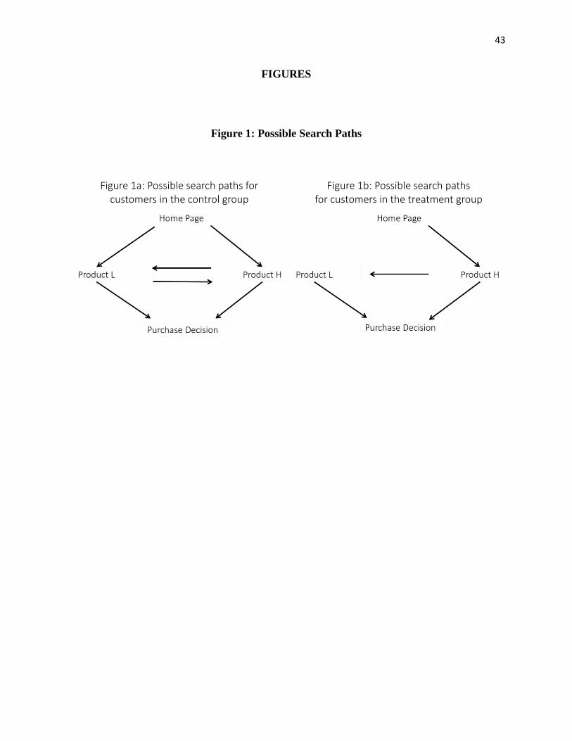
customer to incur a search cost to view the low-priced product. Figure 1 provides an illustration
of possible search paths in our theoretical framework and how they are related to the customers
in the treatment and control groups in our field experiments. For ease of exposition and
analogous to our empirical analysis, we will refer to customers offered search paths in Figure 1a
as being in the control group and customers offered search paths in Figure 1b as being in the
treatment group.
[Insert Figure 1 about here.]
Our customer utility and search model within this framework follows recent work in the
search literature that examines obfuscation in settings with monopolistic competition (e.g.
Petrikaitė 2018; Gamp 2016; Armstrong 2016). Specifically, we suppose there is a mass of
consumers that is normalized to one, and each consumer has unit demand and wants to buy at
most one of the two products. The net utility of consumer 𝑖 who buys product 𝑗 is denoted by 𝑢𝑖𝑗,
which equals the difference between her match value 𝜖𝑖𝑗 and the price 𝑝𝑗 of the product, given
the consumer’s price sensitivity2 𝛼 ∈ [0,1]: 𝑢𝑖𝑗 = 𝜖𝑖𝑗 − 𝛼𝑝𝑗.
The match value indicates the valuation of product 𝑗 by consumer 𝑖; it is consumer- and
product-specific. Match values are distributed independently and identically among consumers
and independently among products, and we denote the pdf of 𝜖𝑖𝑗 as 𝑓𝑗(⋅). Product prices are
common knowledge, but match values are only realized when products are inspected (e.g., Gu &
Liu 2013).3 The customer purchases the product that gives her greater utility, as long as it is
2 For ease of exposition, we do not index each consumer’s price sensitivity, 𝛼, and search cost, 𝑠; instead, we
provide results for varying 𝛼 and 𝑠. 3 We follow the established convention in the search literature by modeling match values as random and prices as
common knowledge. This is appropriate in our context because the scenario of interest is one in which the relative
price comparisons are known (i.e., the average price in the sale section is lower than that in the main section),
whereas such a comparison does not necessarily hold for realized match values. We also note that, strictly speaking,
we require that consumers merely have correct expectations of prices rather than full information. We present
empirical evidence in the Caveats and Limitations section that suggests this modeling assumption is appropriate.
14
positive. Since we consider a single, representative consumer in our following exposition, we
will remove the subscript i for brevity.
Note that if the consumer views product 𝑗 first, she is indifferent between continuing to
search product 𝑗′ ≠ 𝑗 if the expected gain from search equals the search cost, i.e.
∫ (𝜖𝑗′ − 𝛼𝑝𝑗′ − 𝜖𝑗 + 𝛼𝑝𝑗)∞
𝜖𝑗′=𝜖𝑗−𝛼𝑝𝑗+𝛼𝑝𝑗′
𝑓𝑗′(𝜖𝑗′)𝑑𝜖𝑗′ = 𝑠
Define 𝑥𝑗′ = 𝜖𝑗 − 𝛼𝑝𝑗 + 𝛼𝑝𝑗′ such that the above is satisfied. If 𝜖𝑗 − 𝛼𝑝𝑗 > 𝑥𝑗′ − 𝛼𝑝𝑗′ then the
expected gain from search is lower than the search cost and the consumer will not search product
𝑗′. However, if 𝜖𝑗 − 𝛼𝑝𝑗 < 𝑥𝑗′ − 𝛼𝑝𝑗′, then it is worthwhile for the consumer to continue
searching. Note that product 𝑗′ has a positive probability of being inspected only if 𝑠 ≤
∫ (𝜖𝑗′ − 𝛼𝑝𝑗′)𝑓𝑗′(𝜖𝑗′)𝑑𝜖𝑗′∞
𝜖𝑗′=𝛼𝑝𝑗′.
Let 𝑈 𝑗 be a random variable representing the customer’s utility if she views product 𝑗
first. The expected utility for a customer in the treatment group is 𝐸[𝑈 𝐻], and the expected utility
for a customer in the control group is max
{𝐸[𝑈 𝐿], 𝐸[𝑈
𝐻]}. Finally, let 𝑑𝑘𝑗 represent the demand
(purchase probability) of product 𝑘 if product 𝑗 is viewed first, and let 𝑑 𝑗 = 𝑑𝐿
𝑗+ 𝑑𝐻
𝑗. We omit
the dependence of these terms on model parameters for brevity.
Impact of Increasing Search Frictions
In this section, we analyze the model to better understand the impact that increasing
search frictions has on two important retail metrics: conversion and revenue. Here, we define
conversion as the probability that the customer purchases one of the two products rather than
choosing the outside option, i.e. 𝑑 𝑗. First, we will prove analytical results and build our intuition
15
for the special case where 𝜖𝑗~𝑖𝑖𝑑 𝑈𝑛𝑖𝑓[0,1] and then extend our analysis and intuition for other
common and non-identical match value distributions in Web Appendix D. Proofs of all results
can be found in Web Appendix F.
As illustrated in Figure 1a, customers in the control group must choose which product to
view first after landing on the home page, whereas customers in the treatment group are forced to
view the high-priced product first.
Lemma 1: When 𝜖𝑗~𝑖𝑖𝑑 𝑈𝑛𝑖𝑓[0,1], 𝐸[𝑈𝐿] ≥ 𝐸[𝑈𝐻].
Lemma 1 specifies that all customers in the control group choose to view the low-priced product
first; thus, we will equate the search path starting with product 𝐿 to customers in the control
group and the search path starting with product 𝐻 to customers in the treatment group. We note
that this is not necessarily the case when the match values are not independent and identically
distributed 𝑈𝑛𝑖𝑓[0,1], and we address this further in Web Appendix D.
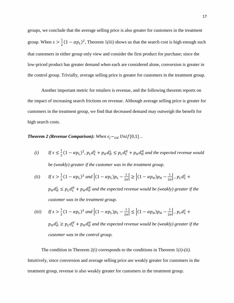
One may naturally hypothesize that conversion in the control group would always be
greater than conversion in the treatment group, i.e. that increasing search frictions for low-priced
products would make them costlier to find and therefore decrease overall conversion. Although
this is sometimes true, the following theorem shows a somewhat surprising result that increasing
search frictions may increase conversion.
Theorem 1 (Conversion Comparison): When 𝜖𝑗~𝑖𝑖𝑑 𝑈𝑛𝑖𝑓[0,1]…
(i) If 𝑠 ≤1
2(1 − 𝛼𝑝𝐻)2, 𝑑
𝐿 = 𝑑 𝐻 and conversion would be the same regardless of if the
customer was in the control or treatment group.

16
(ii) If 1
2(1 − 𝛼𝑝𝐻)2 < 𝑠 ≤
1
2(1 − 𝛼𝑝𝐿)2, 𝑑
𝐿 < 𝑑 𝐻 and conversion would be greater if
the customer was in the treatment group.
(iii) If 𝑠 >1
2(1 − 𝛼𝑝𝐿)2, 𝑑
𝐿 > 𝑑 𝐻 and conversion would be greater if the customer was in
the control group.
Theorem 1(ii) highlights the condition where conversion increases with search frictions.
When 1
2(1 − 𝛼𝑝𝐻)2 < 𝑠 ≤
1
2(1 − 𝛼𝑝𝐿)2, customers in the control group find it too costly to ever
search the high-priced product and thus only consider the low-priced product, whereas customers
in the treatment group may choose to search the low-priced product. Put differently, the search
cost is high enough to force customers in the control group to only consider the low-priced
product for purchase, but not too high to prevent customers in the treatment group from
considering both products for purchase. With more products to choose from, customers in the
treatment group are more likely to make a purchase, resulting in higher conversion. Upon
inspection, we can see that as the consumer’s price sensitivity 𝛼 increases, the range of search
costs for which expected conversion is larger in the treatment group increases and shifts towards
smaller values of 𝑠. Finally, note that the average selling price will be greater for customers in
the treatment group since they are the only ones who purchase the high-priced product with
positive probability.
In contrast, when 𝑠 ≤1
2(1 − 𝛼𝑝𝐻)2, Theorem 1(i) shows us that the search cost is low
enough such that customers in either group will search and consider both products for purchase
before choosing the outside option, and thus there is no difference in conversion. In this case,
since customers in the treatment group view the high-priced product first, they are more likely to
purchase this product than customers in the control group; given conversion is the same for both
17
groups, we conclude that the average selling price is also greater for customers in the treatment
group. When 𝑠 >1
2(1 − 𝛼𝑝𝐿)2, Theorem 1(iii) shows us that the search cost is high enough such
that customers in either group only view and consider the first product for purchase; since the
low-priced product has greater demand when each are considered alone, conversion is greater in
the control group. Trivially, average selling price is greater for customers in the treatment group.
Another important metric for retailers is revenue, and the following theorem reports on
the impact of increasing search frictions on revenue. Although average selling price is greater for
customers in the treatment group, we find that decreased demand may outweigh the benefit for
high search costs.
Theorem 2 (Revenue Comparison): When 𝜖𝑗~𝑖𝑖𝑑 𝑈𝑛𝑖𝑓[0,1]…
(i) If 𝑠 ≤1
2(1 − 𝛼𝑝𝐿)2, 𝑝𝐿𝑑𝐿
𝐿 + 𝑝𝐻𝑑𝐻𝐿 ≤ 𝑝𝐿𝑑𝐿
𝐻 + 𝑝𝐻𝑑𝐻𝐻 and the expected revenue would
be (weakly) greater if the customer was in the treatment group.
(ii) If 𝑠 >1
2(1 − 𝛼𝑝𝐿)2 and |(1 − 𝛼𝑝𝐿)𝑝𝐿 −
1
2𝛼| ≥ |(1 − 𝛼𝑝𝐻)𝑝𝐻 −
1
2𝛼| , 𝑝𝐿𝑑𝐿
𝐿 +
𝑝𝐻𝑑𝐻𝐿 ≤ 𝑝𝐿𝑑𝐿
𝐻 + 𝑝𝐻𝑑𝐻𝐻 and the expected revenue would be (weakly) greater if the
customer was in the treatment group.
(iii) If 𝑠 >1
2(1 − 𝛼𝑝𝐿)2 and |(1 − 𝛼𝑝𝐿)𝑝𝐿 −
1
2𝛼| ≤ |(1 − 𝛼𝑝𝐻)𝑝𝐻 −
1
2𝛼| , 𝑝𝐿𝑑𝐿
𝐿 +
𝑝𝐻𝑑𝐻𝐿 ≥ 𝑝𝐿𝑑𝐿
𝐻 + 𝑝𝐻𝑑𝐻𝐻 and the expected revenue would be (weakly) greater if the
customer was in the control group.
The condition in Theorem 2(i) corresponds to the conditions in Theorem 1(i)-(ii).
Intuitively, since conversion and average selling price are weakly greater for customers in the
treatment group, revenue is also weakly greater for customers in the treatment group.

18
Alternatively, when 𝑠 >1
2(1 − 𝛼𝑝𝐿)2, conversion is greater for the control group, yet average
selling price is greater for the treatment group, and Theorem 2(ii)-(iii) highlights the conditions
under which the additional revenue gain from showing the high-priced product first outweighs
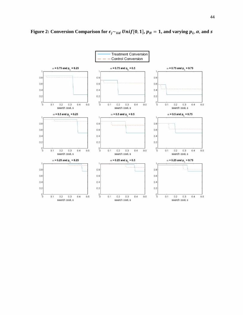
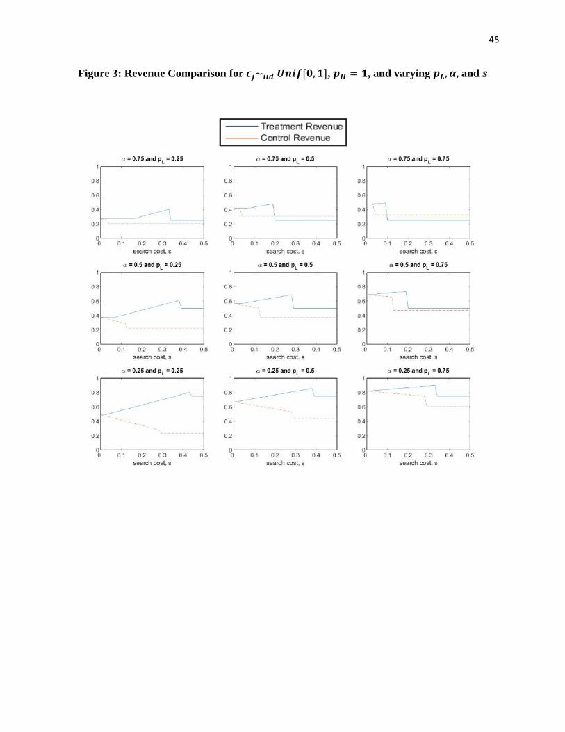
the decrease in conversion and when it does not. Figures 2 and 3 illustrate the magnitude of
conversion and revenue for customers in the treatment and control groups for varying model
parameters.
To summarize our analysis, we find that increasing search frictions may lead to higher or
lower conversion and revenue, depending on the magnitude of the search cost. For low search
costs, we find that conversion is identical and revenue is greater due to increased search frictions.
For moderate search costs, we find that conversion and revenue are both greater due to increased
search frictions. For high search costs, we find that conversion declines but revenue may or may
not decline due to increased search frictions. The relative ranges of search costs (low, moderate,
and high) shift as a function of the consumer’s price sensitivity 𝛼, and in particular, these ranges
shift towards smaller search costs as consumers become more price sensitive; Figure 2 helps
illustrate this observation. Our extended analysis in Web Appendix D suggests that our results
are robust even under other, non-identical match value distributions. Given that the ranges of
low, moderate, and high search costs—and even the search cost itself—are difficult for a retailer
to estimate in practice, the remainder of the paper reports on field experiments we conducted to
estimate the impact of increasing search frictions on conversion and revenue in practice. With
this theoretical framework in mind, we can better understand and interpret the results of our
experiment.
19
FIELD EXPERIMENT I
In our first experiment, we seek preliminary evidence that specific changes to website design can
have significant effects on shopper behavior and purchase outcomes. We vary the presence of
website features that potentially facilitate shopper inspection of discounted items. We include
only new visitors to the desktop version of the online store in order to mitigate potentially
negative effects on the firm’s performance and to control for prior information among
consumers. In evaluating the outcomes, we are particularly interested in the treatment effects on
the discount levels of completed transactions and conversion.
We run the experiment on the retailer’s website over a period of nine days.4 During this
period, all new visitors to the website were randomly assigned to the control group or one of
three treatment groups with equal probability. New visitors are defined as customers who do not
have the website’s cookies on their computers and sign up for a new account before making any
purchase. Only visitors who were using a desktop, laptop, or tablet computer were included in
the study. In total, 104,605 shoppers were included in the experiment. Posterior randomization
checks confirm that the firm correctly implemented the randomization of new visitors to
treatment and control groups. (See Table W3 in Web Appendix E for randomization checks.)
Additionally, only consumers who arrived at the site via the main landing page are
included; we exclude consumers who visit the site via an email coupon, newsletter, or link from
a third-party website. During the experiment no other changes were made to the website.
Descriptions of the control and treatment conditions follow. In each of the treatment conditions,
neither the available product assortment nor any product prices were different from the control
4 Field Experiment I ran on June 17-June 25, 2015.
20
condition.
Control
The control condition is simply the website as is at the time of the study. The website
features elements designed to facilitate consumer search for discounted items. Customers have
three ways to find discounted items: clicking on a prominent link from the landing page to the
outlet catalog, sorting products according to discount level in each catalog through a drop-down
option, and viewing markers that highlight discounts above 40% (see Figure W19 in Web
Appendix E). In each of the treatment conditions, we eliminate each of these elements with the
objective of reordering consumers’ search paths and increasing the required effort to locate
discounted items.
Treatment 1: No link to outlet catalog from main landing page
In this condition, we eliminate the most direct path to discounted items: the outlet link
from the landing page. The remaining links to the outlet catalog are within the website’s sale
section, requiring at least one additional click from a shopper to arrive at the outlet catalog
relative to those in the control group. In line with our theoretical framework, this would require
consumers to view higher-priced items before viewing items with the largest discounts.
Treatment 2: No discount filter and no discount markers
Here we remove the ability of consumers to order product listings according to discount
percentages. We also remove the accompanying discount markers, which provide visual cues for
identifying high discounts. These elements are widely used together by online retailers to
facilitate shopper search and navigation. Similarly to Treatment 1, this would cause consumers to
load pages with higher-priced items first.
Treatment 3: No outlet link, no discount filter, and no discount markers

21
In our third treatment we simultaneously remove all website elements taken out
piecemeal in the first two treatments. Our objective is to induce variation across our treatments in
the magnitude of the search cost associated with inspecting discounted items. As with the first
two treatments, visitors can still find discounted items with the requisite effort in typical
locations throughout the site. Eliminating links, filters, and markers merely adds to the number
of clicks, browsing time, and page views required to locate discounted items.
Evaluation
In evaluating the effects of each treatment we consider several outcome variables5:
1. Average discount: the average ratio of selling prices to original prices6 over items bought
in each treatment group. Given that each treatment makes locating discounts more
difficult, we expect percent discounts to be lower in treatment conditions relative to the
control on average. We use this variable in place of selling prices as a means of enabling
a consolidated presentation of results given the multi-category setting.
2. Percent full-priced purchases: the proportion of purchased items sold without
discounting. Historically, about 50% of purchases on the website are made at full price.
Similarly to the average discount, an increase in this variable in our treatment groups
would be supportive of our hypothesis.
3. Average selling price: the average selling price of all items sold. Similarly to average
discount and percent full-priced purchases, an increase in this variable in our treatment
groups would be supportive of our hypothesis and results from our theoretical analysis.
5 We note that two of our outcome variables (average discount and percent full-priced purchases) are defined
conditional on purchase; hence, they are computed using selected samples by construction. While not ideal for
evaluating experimental results, this is a direct consequence of the behavior being studied and is in line with our
theoretical framework (e.g. Sahni, Wheeler & Chintagunta 2018). 6 The firm does not inflate original prices.
22
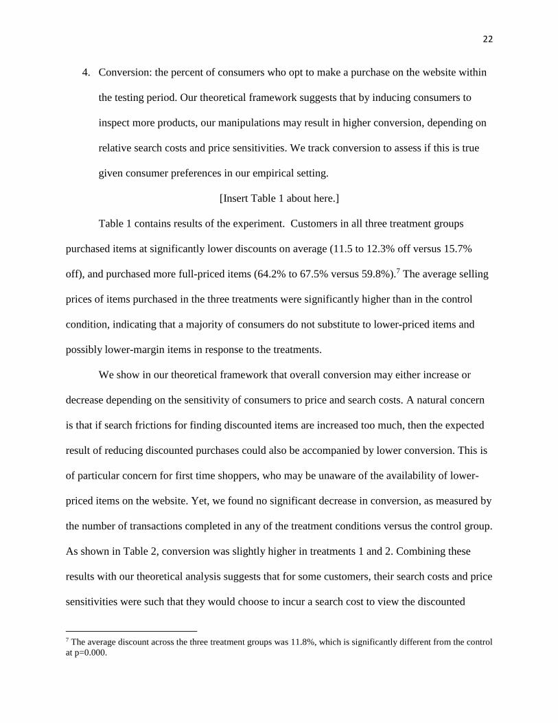
4. Conversion: the percent of consumers who opt to make a purchase on the website within
the testing period. Our theoretical framework suggests that by inducing consumers to
inspect more products, our manipulations may result in higher conversion, depending on
relative search costs and price sensitivities. We track conversion to assess if this is true
given consumer preferences in our empirical setting.
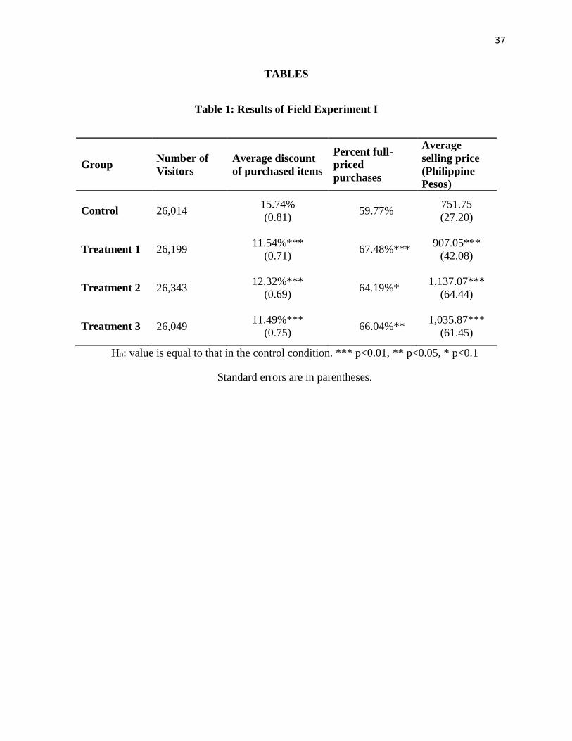
[Insert Table 1 about here.]
Table 1 contains results of the experiment. Customers in all three treatment groups
purchased items at significantly lower discounts on average (11.5 to 12.3% off versus 15.7%
off), and purchased more full-priced items (64.2% to 67.5% versus 59.8%).7 The average selling
prices of items purchased in the three treatments were significantly higher than in the control
condition, indicating that a majority of consumers do not substitute to lower-priced items and
possibly lower-margin items in response to the treatments.
We show in our theoretical framework that overall conversion may either increase or
decrease depending on the sensitivity of consumers to price and search costs. A natural concern
is that if search frictions for finding discounted items are increased too much, then the expected
result of reducing discounted purchases could also be accompanied by lower conversion. This is
of particular concern for first time shoppers, who may be unaware of the availability of lower-
priced items on the website. Yet, we found no significant decrease in conversion, as measured by
the number of transactions completed in any of the treatment conditions versus the control group.
As shown in Table 2, conversion was slightly higher in treatments 1 and 2. Combining these
results with our theoretical analysis suggests that for some customers, their search costs and price
sensitivities were such that they would choose to incur a search cost to view the discounted
7 The average discount across the three treatment groups was 11.8%, which is significantly different from the control
at p=0.000.
23
products if assigned to a treatment group, but would not incur a search cost to view the full-
priced products if assigned to the control group (analogous to condition (ii) in Theorem 1).
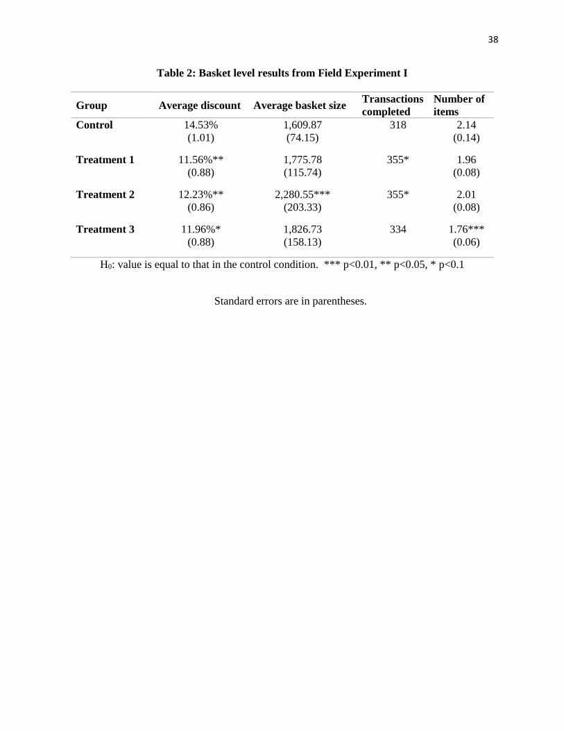
As a robustness check, we performed a comparison across treatments and control groups
at the basket level (versus item level) to compare differences in shopping behavior with respect
to total purchase value and composition decisions. Confirming the main item-level results, Table
2 shows that the average discount of purchase baskets in two out of the three treatments is
significantly lower than for the control group (11.6 to 12.2% versus 14.5%). For treatment 3, it is
marginally significantly lower. Average basket sizes in any of the treatment groups are not
significantly smaller than the control group, although in treatment 3 there were fewer items in
each basket on average.
[Insert Table 2 about here]
These results provide supporting evidence for our hypothesis and demonstrate that our
manipulations have a measurable impact on consumer choice. Given that discounts in fashion
and apparel retail are directly tied to gross margins, our results additionally show that online
retailers can increase their margins without sacrificing conversion by slightly increasing search
frictions associated with their discounted offers. (See Table W4 in Web Appendix E for
measurements of the impact on profitability of the treatment conditions.)
In a setting without search frictions, we contend that consumers inspect discounted
options “for free.” By increasing search frictions, online retailers can direct consumers toward
full-priced options while still making discounted options available for price-sensitive shoppers
willing to incur the extra search cost to find them. In the following sections, we verify that such
heterogeneous treatment effects underlie our main results.

24
FIELD EXPERIMENT II
In our second experiment we investigate the pattern in which shopper responses to added search
frictions vary according to price sensitivity and their familiarity with the retailer. Analogous to
Field Experiment I, we expose consumers to different versions of the online store, each with a
manipulation designed to increase search frictions. We compare the impact of the treatments
versus control on retailer performance measures and use consumer purchase histories to
characterize the heterogeneity in shopper responses. In addition, this experiment also serves as a
replication of our first experiment, run during a sale season approximately one year afterward
with a wider set of treatments and a broader set of subjects.
Experimental Design
We ran this experiment for two weeks on the desktop and tablet versions of the online
store. All consumers were randomly assigned to either the control group or to one of four
treatment groups with equal probability. Whereas in Field Experiment I we included only new
visitors entering through the main landing pages, here we include new as well as returning
consumers regardless of which page they view first. This is a strong test of our model-based
predictions as it seeks to find the conjectured shopper behavior in a population with presumably
high variation in information. A total of 348,110 visitors are included in this experiment (see
Table W6 in Web Appendix E for randomization checks.) The treatment conditions are as
follows:
Treatment 1: Removal of links from main pages to outlet and sale sections of the website
Treatment 2: Removal of discount markers
25
Treatment 3: Removal of discount sorting option
Treatment 4: Replacement of discount-oriented banners with non-discount oriented banners
In contrast to Field Experiment I, we assign the removal of discount markers and sorting
options into two different treatments to separately measure the effects of each intervention. We
also add a fourth treatment, the use of non-discount-oriented banners throughout the site (see
Figure W22 in Web Appendix E for examples of discount banners). In practice, discount-
oriented banners serve a dual purpose: to communicate the existence of marked down items as
well as a navigation tool to access the relevant product listings.
The design of specific discount and replacement banners can introduce additional factors
that may impact our results. Similar, if less pronounced, contamination is present in each of our
other manipulations, particularly since correlation between discounts and non-price attributes are
likely to be nonzero. Given the nature of our proposed mechanism and natural constraints in the
field experiment setting, we cannot completely eliminate these confounds; however, we seek to
mitigate them by including multiple variations between treatments.
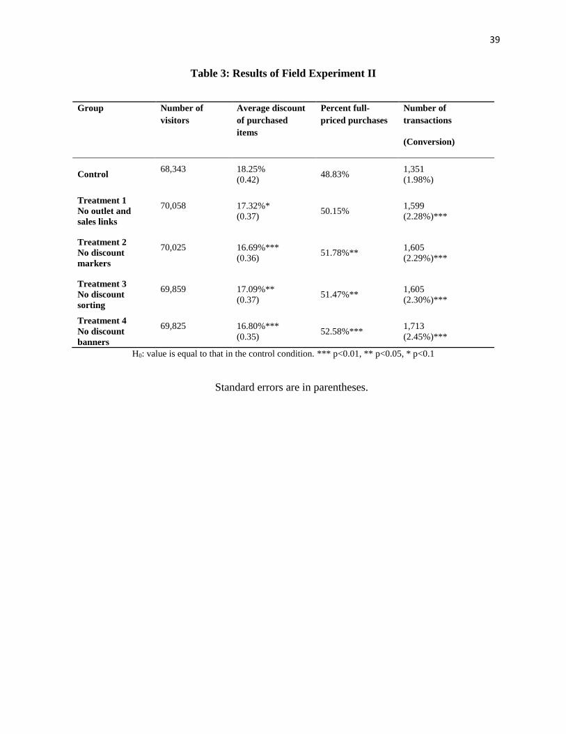
[Insert Table 3 about here.]
Results
Before assessing the impact of price sensitivity on shoppers’ propensities to find and buy
discounted items, we conduct the same analysis as in Table 1, which pools all types of
consumers and present the results in Table 3. Further validating the main findings in Field
Experiment I, this time including existing and new customers, we find that removing discount
markers, sorting by discount and discount-oriented banners (Treatments 2 to 4) decreases both
the average discount of items purchased as well as the incidence of purchasing items on
26
discount.8 As before, this is achieved without a decrease in conversion. An exception to this, and
counter to the findings in Field Experiment I, is the null effect of the removal of outlet and sales
links from the home page (Treatment 1). A possible explanation is that current customers were
not as deterred as new shoppers from finding the high discounts, in the sense of differences in
perceived search costs.9 With the exception of this treatment, the addition of search costs impacts
new and current customers in a qualitatively very similar manner.
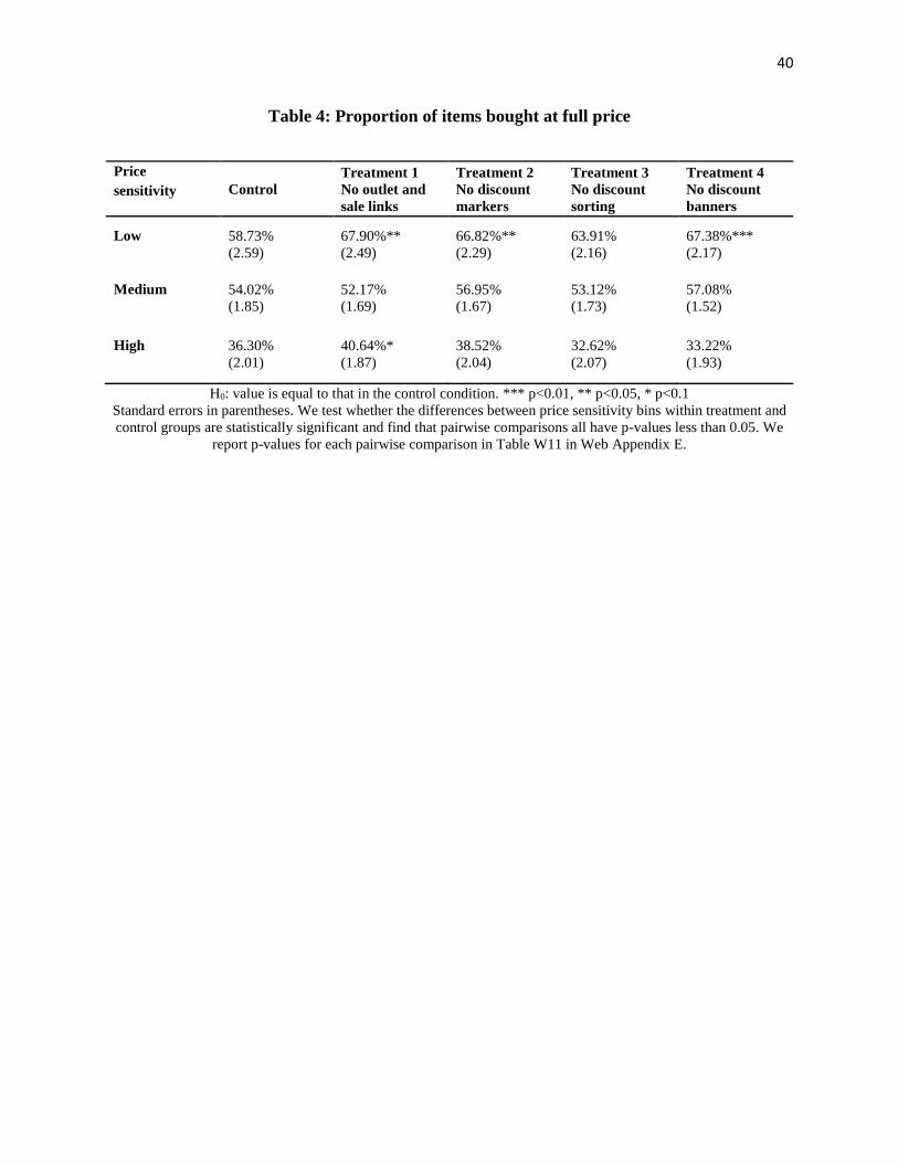
[Insert Table 4 about here.]
Next, we measure the interaction between shoppers’ price sensitivity and their
willingness to incur search costs to find discounted items. We classify existing customers
according to their price sensitivity using historical transaction data. (Details are in Appendix A.)
While using observational data as we do to infer price sensitivity has limitations, we note that
any deficiency in predictive accuracy would bias our results toward a false negative in detecting
heterogeneous treatment effects.
In Table 4, we group consumers into three quantiles according to their price sensitivity as
indicated by predicted values from the full model (column 4 of Table A3 in the appendix). In an
additional validation of our classification model, we find that low price sensitivity consumers are
directionally more likely to purchase full-priced items in all treatment groups (first row). In three
of four treatment groups, we observe statistically significant increases in the proportion of full-
priced items bought by customers with low price sensitivity. Equally notable, this is not the case
for medium or high price sensitivity consumers, who willingly incur search costs to avail of
8 The average discount across the three treatment groups was 17.0%, which is significantly different from the
average discount in the control condition of 18.2% at p=0.0042. 9 See Web Appendix C for a description of the difference in outcomes for new versus existing customers.
27
discounts. This result provides additional evidence, by including current users and adding other
forms of search costs to the website, that online retailers can improve their margins and, thus,
profitability, by deliberately adding small frictions to the shopping process. We present actual
profitability measures in Table W7 in Web Appendix E using item-level marginal cost data
provided by the firm.
Our theoretical framework posits that higher conversion is a consequence of more
products inspected in regions of moderate search costs. Unfortunately, we lack the granular data
required to precisely measure the number of products inspected by consumers. We do, however,
have access to aggregate data on browsing behavior available through the firm’s web analytics
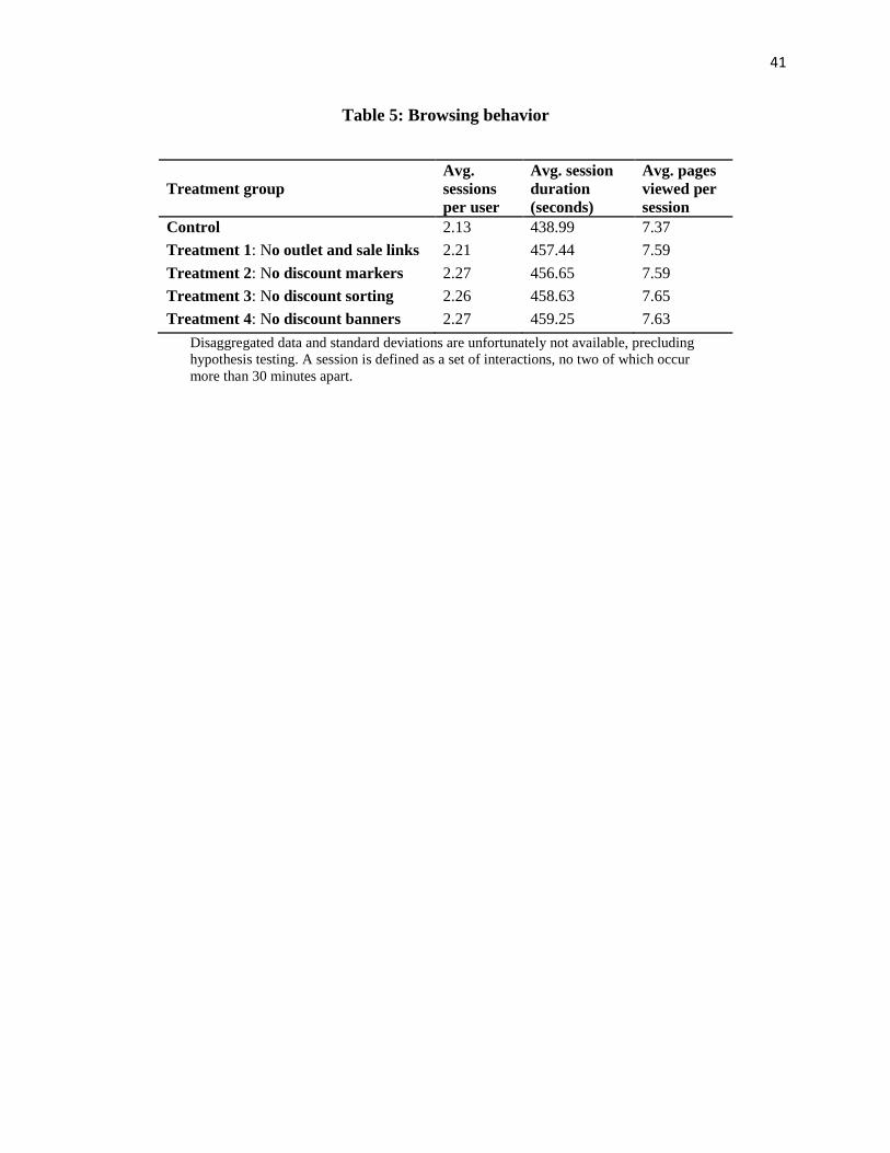
provider. Table 5 presents key measures of browsing behavior across each treatment group. On
average, visitors falling within each treatment group visited the website more times during the
testing period, spent more time during each visit, and viewed more pages. These are consistent
with our proposed mechanism for employing search frictions. Specifically, locating discounted
items would necessarily involve more time spent on the website in the treatment conditions. As
suggested by our theoretical analysis, we conjecture that these changes in browsing behavior
may have concurrently resulted in shoppers considering a broader set of products, thus leading to
higher conversion.
[Insert Table 5 about here.]
Caveats and Limitations
Our two field experiments provide convergent evidence that increasing search frictions
may be profitable for a monopolistic online seller in the short run. While we replicate our results
under different demand conditions and consumer profiles, natural questions remain pertaining to
28
alternative explanations for our empirical findings, the generalizability of our results to other
online retail contexts, and the long-term viability of increasing search frictions. In this subsection
we provide suggestive evidence that points to probable answers to some of these questions, and
to potential directions for future research.
While the results of our experiments conform to the main predictions of our theoretical
framework, the nature of our empirical setting allows for alternative explanations to potentially
be at play. A few such mechanisms arise when our assumption that consumers have rational
expectations is violated. If, contrary to our assumptions, consumers have mistaken beliefs about
product quality or prices, then inducing them to take alternative search paths may cause them to
change their purchase behavior by updating their beliefs. Alternatively, consumers may update
their priors about outside options differently depending on their realized search patterns.
Another potential factor that we do not account for are store-level preferences that may
be influenced by our treatments. For instance, customers who do not see links to sale or outlet
sections may perceive the firm as being of higher quality than those in the control condition. The
elimination of links in our treatment conditions may also simply present a more pleasing
interface, thus resulting in better sales results.
We are constrained in our ability to determine how important these alternative accounts
are relative to that laid out in our model. Some of these constraints are natural, such as our
inability to measure consumer beliefs; others pertain to data limitations, such as our lack of
clickstream data. One source of variation in the data we can inspect is that between new and
existing customers. There is a reasonable expectation that, relative to existing customers, new
customers have less information about firm and product attributes.
29
We explore the differences in results between new and existing customers and find no
systematic differences (see Figure W2, Table W9, and Table W10 in Web Appendix C and E).
Our treatments appear to increase both conversion and the proportion of full-priced purchases
among both groups at comparable margins. This suggests that information updating likely has a
limited role in generating our experimental results. Furthermore, it suggests that both new and
existing consumers have reasonable expectations on prices offered by the retailer, in line with
our theoretical model. Nonetheless, we recognize that the mechanism we emphasize in this paper
is unlikely to fully account for our experimental results.
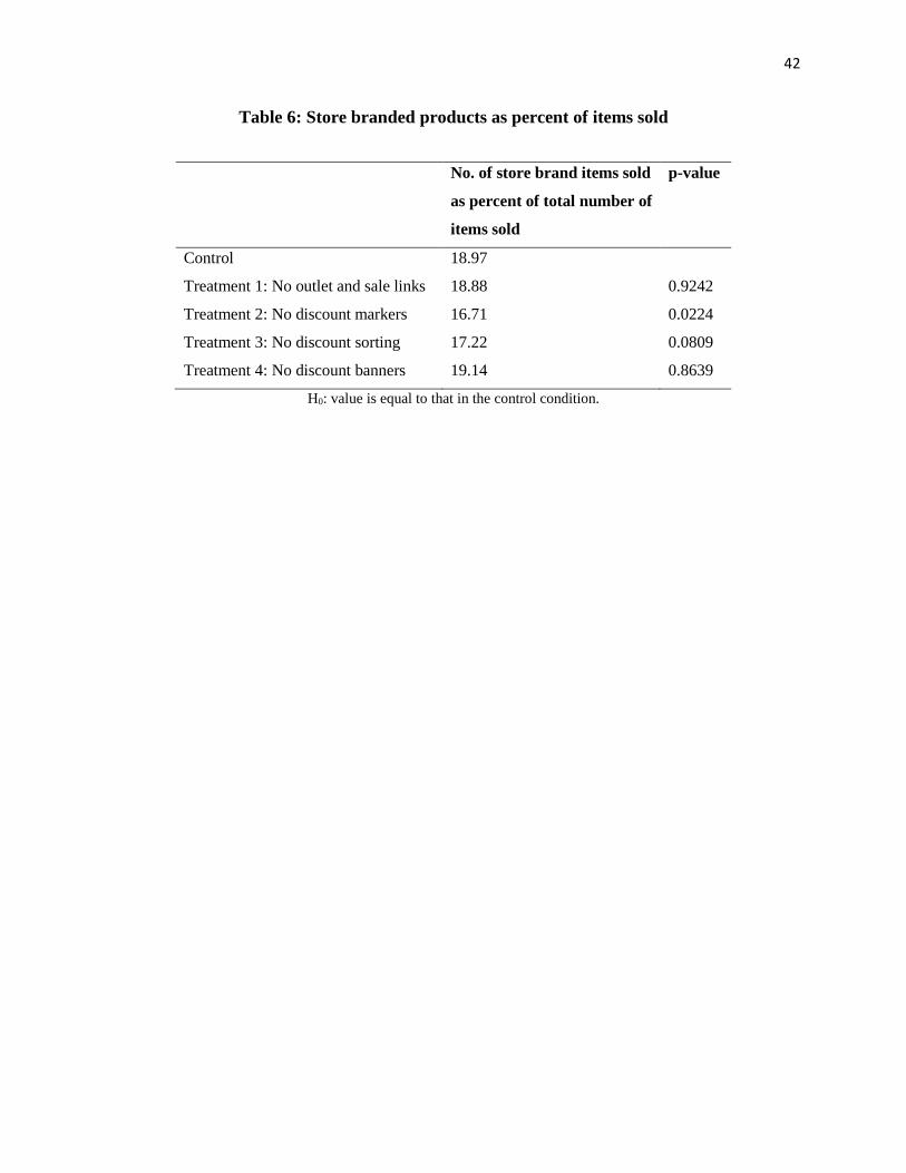
We consider the conjecture that increasing search frictions may cause consumers to
switch to alternatives in the presence of competing firms. While our data provider has no similar-
sized competitors online, they offer items under a private label in addition to items from national
and global brands. The firm faces less competition for its private label products, which are
available only on their online store, than for the rest of its products, which are available from
offline sellers. We examine the outcomes within each of these categories in an effort to find
evidence of heterogeneous treatment effects, which would be indicative of the role of
competition. If consumers are prone to switching to competitors upon facing added search
frictions, then they should be more likely to buy store brand products in the treatment conditions.
Table 6 presents the portion of items sold in each treatment group that are store brand products.
[Insert Table 6 about here.]
We find that in none of the treatment conditions is the ratio of store brand to
national/global brand items sold significantly higher than in the control, which suggests that the
30
presence of competitors for branded products does not play a significant role in mitigating our
results within this setting.
We turn our attention to the potential long run effects of increasing search frictions in an
online store. Transaction and web browsing data are available for several periods beyond the end
of our experimentation, and may point to specific long run effects. We consider cohorts of
consumers falling into each of the randomly assigned groups from Field Experiment II and track
their revisit rates and conversion over time. Table W8 in Web Appendix E shows the number of
consumers who visited the website during our sample period of two weeks in 2016. For each
half-month period thereafter, until the end of the year, we list the number of users from the
original sample who visit the website and corresponding conversion.
We find no evidence that consumers in the treatment conditions had lower revisit rates
than that in the control. In fact, for every month and treatment group, the revisit rate is higher
among the treatment cohorts than in the control cohorts at p < 0.01. Qualitatively similar
measurements are obtained from groups in Field Experiment I. This is perhaps unsurprising
given that the conversion was higher in the treatment groups compared to the control group,
implying that customers were able to more successfully find products they like and are therefore
more likely to be return shoppers. Interestingly, this suggests the possibility that increasing
search frictions leads to improvements in customer satisfaction and retention.
31
CONCLUSION
Online retail represents a rapidly growing proportion of overall retail sales. However,
margins in online retail can often be smaller than in offline retail. One conjecture for this
discrepancy is that online sellers are less able to price discriminate compared to their offline
counterparts. In this paper, we explore how deliberately imposing additional search costs on
online shoppers can improve gross margins by increasing the number of items inspected and
serving as a sorting mechanism among customers.
We find encouraging evidence that minor changes to the design of an online store can
substantially improve its margins and profitability. By increasing search frictions in simple
ways—removing selected links, narrowing down product sorting options, and limiting visual
markers—online sellers can achieve more full-priced sales from price-insensitive shoppers who
face higher search costs. As a result, the average selling price increases due to a higher
proportion of full-priced items sold.
Our theoretical model shows how increasing search frictions may either increase or
decrease conversion depending on consumer preferences. Through our field experiments, we
find that conversion increases upon the addition of search frictions in a typical online retail
setting. Inspecting browsing behavior in the treatment groups suggests that as visitors spend
more time on the website given higher search frictions, they may also be considering a larger set
of products.
Our results have direct implications for online sellers. Without changes to product prices
or assortment, online sellers can improve their margin performance by implementing subtle
changes to website design. We note with particular excitement that this is a low-cost
32
manipulation with low data requirements, and one that can deliver large gains in margin. Our
findings imply that by indiscriminately prioritizing ease of search and purchase, online sellers
may be giving up gross margins by unwittingly giving away discounts to price-insensitive
consumers and curtailing consumer exploration of the product assortment.
Our research also suggests that some online browsing behavior can be effortful or time-
consuming enough for shoppers to prefer paying higher prices. We consider it a fruitful area for
future research to determine which specific properties of online interaction consumers find most
effortful. This can provide helpful guidance for a wide array of applications, from online store
design to digital advertising.
33
REFERENCES
Armstrong, Mark. "Ordered consumer search." Journal of the European Economic
Association 15.5 (2017): 989-1024.
Bakos, J. Yannis. "Reducing buyer search costs: Implications for electronic
marketplaces." Management science 43.12 (1997): 1676-1692.
Bell, David R., Teck-Hua Ho, and Christopher S. Tang. "Determining where to shop: Fixed and
variable costs of shopping." Journal of Marketing Research (1998): 352-369.
Brown, Jennifer, Tanjim Hossain, and John Morgan. "Shrouded attributes and information
suppression: Evidence from the field." The Quarterly Journal of Economics 125.2 (2010): 859-
876.
Brynjolfsson, Erik, and Michael D. Smith. "Frictionless commerce? A comparison of Internet
and conventional retailers." Management Science 46.4 (2000): 563-585.
Choi, Hana, and Carl F. Mela. "Online marketplace advertising." (2016).
Coughlan, Anne T., and David A. Soberman. "Strategic segmentation using outlet
malls." International Journal of Research in Marketing 22.1 (2005): 61-86.
De los Santos, Babur, and Sergei Koulayev. “Optimizing click-through in online rankings with
endogenous search refinement.” Marketing Science 36.4 (2017): 542-564.
Ellison, Glenn, and Sara Fisher Ellison. "Lessons about Markets from the Internet." Journal of
Economic Perspectives 19.2 (2005): 139-158.
Ellison, Glenn, and Sara Fisher Ellison. "Search, obfuscation, and price elasticities on the
internet." Econometrica 77.2 (2009): 427-452.
Ellison, Glenn, and Alexander Wolitzky. "A search cost model of obfuscation." The RAND
Journal of Economics 43.3 (2012): 417-441.
Gamp, Tobias. "Guided search." Working paper (2016).
34
Gu, Zheyin, and Yunchuan Liu. "Consumer fit search, retailer shelf layout, and channel
interaction." Marketing Science 32.4 (2013): 652-668.
Hui, Sam K., J. Jeffrey Inman, Yanliu Huang, and Jacob Suher (2013), “The Effect of In-Store
Travel Distance on Unplanned Spending: Applications to Mobile Promotion
Strategies,” Journal of Marketing, 77(2), 1-16.
Jing, Bing. "Lowering Customer Evaluation Costs, Product Differentiation, and Price
Competition." Marketing Science 35.1 (2015): 113-127.
Kim, Byung-Do, Kannan Srinivasan, and Ronald T. Wilcox. "Identifying price sensitive
consumers: the relative merits of demographic vs. purchase pattern information." Journal of
Retailing 75.2 (1999): 173-193.
Kopalle, Praveen, et al. "Retailer pricing and competitive effects." Journal of Retailing 85.1
(2009): 56-70.
Lal, Rajiv, and David E. Bell. "The impact of frequent shopper programs in grocery
retailing." Quantitative Marketing and Economics 1.2 (2003): 179-202.
Lambrecht, Anja, and Bernd Skiera. "Paying too much and being happy about it: Existence,
causes, and consequences of tariff-choice biases." Journal of Marketing Research 43.2 (2006):
212-223.
Leslie, Phillip. "Price discrimination in Broadway theater." RAND Journal of Economics (2004):
520-541.
Lynch Jr, John G., and Dan Ariely. "Wine online: Search costs affect competition on price,
quality, and distribution." Marketing science 19.1 (2000): 83-103.
McManus, Brian. "Nonlinear pricing in an oligopoly market: The case of specialty coffee." The
RAND Journal of Economics 38.2 (2007): 512-532.
Monga, Ashwani, and Ritesh Saini. "Currency of search: How spending time on search is not the
same as spending money." Journal of Retailing 85.3 (2009): 245-257.
35
Mussa, Michael, and Sherwin Rosen. "Monopoly and product quality." Journal of Economic
Theory 18.2 (1978): 301-317.
Narasimhan, Chakravarthi. "A price discrimination theory of coupons." Marketing Science 3.2
(1984): 128-147.
Narayanan, Sridhar, and Kirthi Kalyanam. "Position effects in search advertising and their
moderators: A regression discontinuity approach." Marketing Science 34.3 (2015): 388-407.
Ngwe, Donald. "Why outlet stores exist: Averting cannibalization in product line
extensions." Marketing Science 36.4 (2017): 523-541.
Nichols, Donald, Eugene Smolensky, and T. Nicolaus Tideman. "Discrimination by waiting time
in merit goods." The American Economic Review 61.3 (1971): 312-323.
Petrikaitė, Vaiva. "Consumer obfuscation by a multiproduct firm." The RAND Journal of
Economics 49.1 (2018): 206-223.
Ratchford, Brian T. "Online pricing: review and directions for research." Journal of Interactive
Marketing 23.1 (2009): 82-90.
Rigby, Darrell. "The future of shopping." Harvard Business Review 89.12 (2011): 65-76.
Sahni, Navdeep S., S. Christian Wheeler, and Pradeep Chintagunta. "Personalization in Email
Marketing: The Role of Noninformative Advertising Content." Marketing Science,
forthcoming.
Seiler, Stephan, and Fabio Pinna. "Estimating search benefits from path-tracking data:
measurement and determinants." Marketing Science 36.4 (2017): 565-589.
Seim, Katja, Maria Ana Vitorino, and David M. Muir. "Do consumers value price
transparency?" Quantitative Marketing and Economics 15.4 (2017): 305-339.
Stahl, Dale O. "Oligopolistic pricing with sequential consumer search." The American Economic
Review (1989): 700-712.
36
Ursu, Raluca. "The power of rankings: Quantifying the effect of rankings on online consumer
search and purchase decisions." Marketing Science, forthcoming.
U.S. Census Bureau News. 2018.
https://www.census.gov/retail/mrts/www/data/pdf/ec_current.pdf. Accessed January 23, 2019.
Van Heerde, Harald J., Els Gijsbrechts, and Koen Pauwels. "Winners and losers in a major price
war." Journal of Marketing Research 45.5 (2008): 499-518.
Varian, Hal R. "A model of sales." The American Economic Review 70.4 (1980): 651-659.
Weitzman, Martin L. "Optimal search for the best alternative." Econometrica: Journal of the
Econometric Society (1979): 641-654.
Wilson, Chris M. "Ordered search and equilibrium obfuscation." International Journal of
Industrial Organization 28.5 (2010): 496-506.
37
TABLES
Table 1: Results of Field Experiment I
Group Number of
Visitors
Average discount
of purchased items
Percent full-
priced
purchases
Average
selling price
(Philippine
Pesos)
Control 26,014 15.74%
(0.81) 59.77%
751.75
(27.20)
Treatment 1 26,199 11.54%***
(0.71) 67.48%***
907.05***
(42.08)
Treatment 2 26,343 12.32%***
(0.69) 64.19%*
1,137.07***
(64.44)
Treatment 3 26,049 11.49%***
(0.75) 66.04%**
1,035.87***
(61.45)
H0: value is equal to that in the control condition. *** p<0.01, ** p<0.05, * p<0.1
Standard errors are in parentheses.
38
Table 2: Basket level results from Field Experiment I
Group Average discount Average basket size Transactions
completed
Number of
items
Control 14.53%
(1.01)
1,609.87
(74.15)
318 2.14
(0.14)
Treatment 1 11.56%**
(0.88)
1,775.78
(115.74)
355* 1.96
(0.08)
Treatment 2 12.23%**
(0.86)
2,280.55***
(203.33)
355* 2.01
(0.08)
Treatment 3 11.96%*
(0.88)
1,826.73
(158.13)
334 1.76***
(0.06)
H0: value is equal to that in the control condition. *** p<0.01, ** p<0.05, * p<0.1
Standard errors are in parentheses.
39
Table 3: Results of Field Experiment II
Group Number of
visitors
Average discount
of purchased
items
Percent full-
priced purchases
Number of
transactions
(Conversion)
Control 68,343 18.25%
(0.42) 48.83%
1,351
(1.98%)
Treatment 1
No outlet and
sales links
70,058 17.32%*
(0.37) 50.15%
1,599
(2.28%)***
Treatment 2
No discount
markers
70,025 16.69%***
(0.36) 51.78%**
1,605
(2.29%)***
Treatment 3
No discount
sorting
69,859 17.09%**
(0.37) 51.47%**
1,605
(2.30%)***
Treatment 4
No discount
banners
69,825 16.80%***
(0.35) 52.58%***
1,713
(2.45%)***
H0: value is equal to that in the control condition. *** p<0.01, ** p<0.05, * p<0.1
Standard errors are in parentheses.
40
Table 4: Proportion of items bought at full price
Price
sensitivity Control
Treatment 1
No outlet and
sale links
Treatment 2
No discount
markers
Treatment 3
No discount
sorting
Treatment 4
No discount
banners
Low 58.73%
(2.59)
67.90%**
(2.49)
66.82%**
(2.29)
63.91%
(2.16)
67.38%***
(2.17)
Medium 54.02%
(1.85)
52.17%
(1.69)
56.95%
(1.67)
53.12%
(1.73)
57.08%
(1.52)
High 36.30%
(2.01)
40.64%*
(1.87)
38.52%
(2.04)
32.62%
(2.07)
33.22%
(1.93)
H0: value is equal to that in the control condition. *** p<0.01, ** p<0.05, * p<0.1
Standard errors in parentheses. We test whether the differences between price sensitivity bins within treatment and
control groups are statistically significant and find that pairwise comparisons all have p-values less than 0.05. We
report p-values for each pairwise comparison in Table W11 in Web Appendix E.
41
Table 5: Browsing behavior
Treatment group
Avg.
sessions
per user
Avg. session
duration
(seconds)
Avg. pages
viewed per
session
Control 2.13 438.99 7.37
Treatment 1: No outlet and sale links 2.21 457.44 7.59
Treatment 2: No discount markers 2.27 456.65 7.59
Treatment 3: No discount sorting 2.26 458.63 7.65
Treatment 4: No discount banners 2.27 459.25 7.63
Disaggregated data and standard deviations are unfortunately not available, precluding
hypothesis testing. A session is defined as a set of interactions, no two of which occur
more than 30 minutes apart.
42
Table 6: Store branded products as percent of items sold
No. of store brand items sold
as percent of total number of
items sold
p-value
Control 18.97
Treatment 1: No outlet and sale links 18.88 0.9242
Treatment 2: No discount markers 16.71 0.0224
Treatment 3: No discount sorting 17.22 0.0809
Treatment 4: No discount banners 19.14 0.8639
H0: value is equal to that in the control condition.
43
FIGURES
Figure 1: Possible Search Paths
Figure 1a: Possible search paths for customers in the control group
Figure 1b: Possible search paths for customers in the treatment group
44
Figure 2: Conversion Comparison for 𝝐𝒋~𝒊𝒊𝒅 𝑼𝒏𝒊𝒇[𝟎, 𝟏], 𝒑𝑯 = 𝟏, and varying 𝒑𝑳, 𝜶, and 𝒔
45
Figure 3: Revenue Comparison for 𝝐𝒋~𝒊𝒊𝒅 𝑼𝒏𝒊𝒇[𝟎, 𝟏], 𝒑𝑯 = 𝟏, and varying 𝒑𝑳, 𝜶, and 𝒔
46
APPENDIX A: Approximating Price Sensitivity
Our theoretical framework predicts differential effects of search frictions on price-insensitive
versus price-sensitive shoppers. The predicted impact on purchase behavior should
disproportionally affect the former. We develop a parsimonious empirical model of price
sensitivity for shoppers in our setting. Its purpose is to provide us with a means of classifying
consumers according to their baseline appetite for discounts. We use the predicted values of this
model as a proxy for price sensitivity. After estimating the model, we assess its predictive
accuracy by comparing the behavior of pre-classified groups of shoppers in a validation field
experiment.
Data
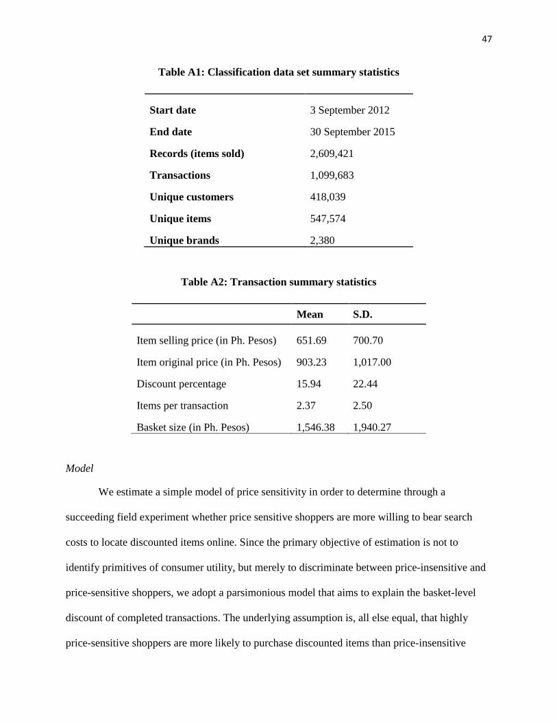
The data for this analysis consists of the retailer’s historical transaction-level sales
records from its inception in September 2012 until September 2015. Over 2.5 million individual
items were sold whereby 418,039 consumers made over one million transactions during that
period. Each record (an item sold) contains shopper attributes, product attributes, and transaction
attributes. Tables A1 and A2 provide a description of the available data and basic transaction-
level summary statistics.
47
Table A1: Classification data set summary statistics
Start date 3 September 2012
End date 30 September 2015
Records (items sold) 2,609,421
Transactions 1,099,683
Unique customers 418,039
Unique items 547,574
Unique brands 2,380
Table A2: Transaction summary statistics
Mean S.D.
Item selling price (in Ph. Pesos) 651.69 700.70
Item original price (in Ph. Pesos) 903.23 1,017.00
Discount percentage 15.94 22.44
Items per transaction 2.37 2.50
Basket size (in Ph. Pesos) 1,546.38 1,940.27
Model
We estimate a simple model of price sensitivity in order to determine through a
succeeding field experiment whether price sensitive shoppers are more willing to bear search
costs to locate discounted items online. Since the primary objective of estimation is not to
identify primitives of consumer utility, but merely to discriminate between price-insensitive and
price-sensitive shoppers, we adopt a parsimonious model that aims to explain the basket-level
discount of completed transactions. The underlying assumption is, all else equal, that highly
price-sensitive shoppers are more likely to purchase discounted items than price-insensitive
48
shoppers. Categories of explanatory variables for price sensitivity include demographic
characteristics, prior transaction behavior, and shopping conditions known to be associated with
discount-seeking behavior.
These variables were chosen based on availability and management’s expectation of their
relationship to discount purchasing. We run a series of Tobit regressions of most recent average
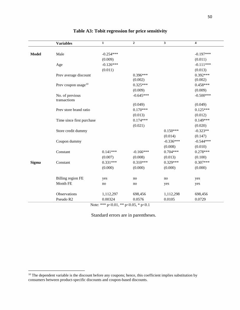
basket discount on these covariates and present estimates in Table A3. As per prior literature, we
use a Tobit model given that discounts are a left-censored (at zero) proxy for price-sensitivity,
our conceptual variable of interest (Lambrecht & Skiera 2006; Van Heerde, Gijsbrechts &
Pauwels 2008). In order to evaluate the relative importance of demographics, prior transaction
behavior, and current shopping conditions, we estimate separate regressions for each subcategory
of explanatory variables in addition to the full model.
Results
In general we find that relationships between consumer attributes, prior shopping
behavior, current shopping conditions, and current shopping behavior are strong and robust to
the usage of different choices of covariates. Each category of explanatory variables
(corresponding to columns in Table A3) improves the ability of the model to predict preference
for discounts. Observed discounts are lower for men and older customers. They are higher for
customers who have previously bought at higher discounts, used coupons, and bought more store
branded items. Meanwhile, discounts are lower for consumers who redeem coupons in the
current purchase instance, use store credit, and have more previously completed transactions.
We use the empirical model estimated in this section to pre-classify shoppers according
to their levels of price sensitivity in order to articulate the mechanism behind our main result in

49
Field Experiment 1. In effect we use all of the available information on consumers to achieve
this classification, assigning weights to each variable according to its estimated coefficient. We
consider this to be an improvement over an ad hoc classification, say, by grouping shoppers
according to the average discount in their purchase histories. However, we also recognize the
shortcomings of this approach owing to the aggregation of information, the lack of information
on visits that result in no purchase, and the changing assortment over time. In order to increase
our confidence in the resulting classification, we seek to establish its external validity. In the next
section, we describe how we validate our classification model by measuring responses to email
newsletters in a field experiment.
50
Table A3: Tobit regression for price sensitivity
Note: *** p<0.01, ** p<0.05, * p<0.1
Standard errors are in parentheses.
10 The dependent variable is the discount before any coupons; hence, this coefficient implies substitution by
consumers between product-specific discounts and coupon-based discounts.
Variables 1 2 3 4
Model Male -0.254***
-0.197*** (0.009)
(0.011)
Age -0.126***
-0.111*** (0.011)
(0.013)
Prev average discount
0.396***
0.392*** (0.002)
(0.002)
Prev coupon usage10
0.325***
0.458*** (0.009)
(0.009)
No. of previous
transactions
-0.645***
-0.500***
(0.049)
(0.049)
Prev store brand ratio
0.170***
0.125*** (0.013)
(0.012)
Time since first purchase
0.174***
0.149*** (0.021)
(0.020)
Store credit dummy
0.150*** -0.323** (0.014) (0.147)
Coupon dummy
-0.336*** -0.544*** (0.008) (0.010)
Constant 0.141*** -0.166*** 0.704*** 0.278*** (0.007) (0.008) (0.013) (0.100)
Sigma Constant 0.331*** 0.310*** 0.329*** 0.307*** (0.000) (0.000) (0.000) (0.000)
Billing region FE yes no no yes Month FE no no yes yes
Observations 1,112,297 698,456 1,112,298 698,456
Pseudo R2 0.00324 0.0576 0.0105 0.0729

51
APPENDIX B: Validation Experiment
We test the external validity of our empirical model of price sensitivity. We send discount and
non-discount oriented email newsletters to randomly assigned consumers and test whether the
classification determined by the Tobit model of the previous section is indeed associated with a
higher response rate for discount (versus non-discount) emails for price-sensitive (versus price-
insensitive) shoppers.
Experimental Design
We include the firm’s entire mailing list of 246,688 consumers in this experiment. A
consumer gets on the mailing list by providing his or her email address to the firm through
registering an account, signing up for updates, or requesting a coupon. Consumers were
randomly assigned to two groups, henceforth Group 1 and Group 2. Each group received a
schedule of both discount- and non-discount-oriented newsletters as presented in Table B1 in
order to counteract day-of-week effects.
Table B1: Schedule of newsletter treatments
Group 1 (50%) Group 2 (50%)
Sunday Control Control
Monday Discount Full price
Tuesday Discount Full price
Wednesday Discount Full price
Thursday Full price Discount
Friday Full price Discount
The control newsletters sent out on Sunday were non-discount oriented and identical
52
between groups whereas, within each day, only the discount versus non-discount messaging was
different between groups. For each newsletter sent, we observe whether the email was opened
and which link within the email, if any, was clicked by the recipient. We also observe all
transactions on the website, which we can link to consumers in the experiment via their email
addresses.
Product categories featured on the email newsletters varied between days, but were kept
constant between control and treatment groups within days. Care was also taken to keep all
creative elements on the newsletters constant, such that only discount messaging (e.g. “up to
40% off”) and any price information varied in the execution. This variation in messaging was
also reflected in the subject line. For an example of a discount and full-price email used, see
Figure W21 in Web Appendix E.
Customers on the mailing list vary in the frequency with which they opt to receive
newsletters. The breakdown is that 62.34% of subscribers receive them every day, 3.32% receive
them three times a week, and 34.35% receive them once a week. Figure W20 in Web Appendix
E shows the daily schedule for each pattern. The newsletter schedule shown in Table B1 was
designed to gain maximum variation among consumers regardless of their frequency as well as
minimize any day-of-week effects.11
In order to establish the validity of the classification of the Tobit model, we generate
predicted values from the model given each consumer’s purchase history prior to the newsletter
experiment in this paper.12 We argue that our model is indicative of price sensitivity if consumers
11 The original plan included a pair of newsletters for Saturday that followed Friday’s pattern; however due to a
server failure the emails were never sent out. 12 Only consumer-specific and purchase history variables (male dummy, customer age, previous discount, previous
coupon dummy, number of previous transactions, store brand purchase ratio, time since first purchase) will be
included in the prediction. The predicted values themselves will have no direct interpretation, but will be treated as
sufficient statistics for price sensitivity.
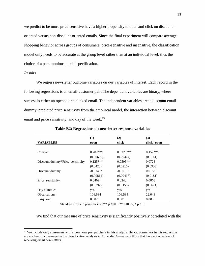
53
we predict to be more price-sensitive have a higher propensity to open and click on discount-
oriented versus non-discount-oriented emails. Since the final experiment will compare average
shopping behavior across groups of consumers, price-sensitive and insensitive, the classification
model only needs to be accurate at the group level rather than at an individual level, thus the
choice of a parsimonious model specification.
Results
We regress newsletter outcome variables on our variables of interest. Each record in the
following regressions is an email-customer pair. The dependent variables are binary, where
success is either an opened or a clicked email. The independent variables are: a discount email
dummy, predicted price sensitivity from the empirical model, the interaction between discount
email and price sensitivity, and day of the week.13
Table B2: Regressions on newsletter response variables
(1) (2) (3)
VARIABLES open click click | open
Constant 0.207*** 0.0328*** 0.152***
(0.00630) (0.00324) (0.0141)
Discount dummy*Price_sensitivity 0.125*** 0.0505** 0.0728
(0.0420) (0.0216) (0.0933)
Discount dummy -0.0149* -0.00103 0.0188
(0.00811) (0.00417) (0.0181)
Price_sensitivity 0.0402 0.0248 0.0868
(0.0297) (0.0153) (0.0671)
Day dummies yes yes yes
Observations 106,534 106,534 22,043
R-squared 0.002 0.001 0.003
Standard errors in parentheses. *** p<0.01, ** p<0.05, * p<0.1
We find that our measure of price sensitivity is significantly positively correlated with the
13 We include only consumers with at least one past purchase in this analysis. Hence, consumers in this regression
are a subset of consumers in the classification analysis in Appendix A—namely those that have not opted out of
receiving email newsletters.
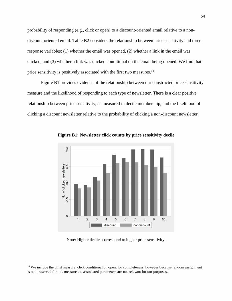
54
probability of responding (e.g., click or open) to a discount-oriented email relative to a non-
discount oriented email. Table B2 considers the relationship between price sensitivity and three
response variables: (1) whether the email was opened, (2) whether a link in the email was
clicked, and (3) whether a link was clicked conditional on the email being opened. We find that
price sensitivity is positively associated with the first two measures.14
Figure B1 provides evidence of the relationship between our constructed price sensitivity
measure and the likelihood of responding to each type of newsletter. There is a clear positive
relationship between price sensitivity, as measured in decile membership, and the likelihood of
clicking a discount newsletter relative to the probability of clicking a non-discount newsletter.
Figure B1: Newsletter click counts by price sensitivity decile
Note: Higher deciles correspond to higher price sensitivity.
14 We include the third measure, click conditional on open, for completeness; however because random assignment
is not preserved for this measure the associated parameters are not relevant for our purposes.
55
Web Appendix of
“The Impact of Increasing Search Frictions on Online Shopping Behavior:
Evidence from a Field Experiment”
WEB APPENDIX A: Variation in non-price attributes
Our theoretical framework assumes the same distribution of non-price attributes for different
price and discount levels. While not crucial to our main results, variation in non-price attributes
may influence the results from our field experiments. For instance, if by re-ordering search paths
we expose consumers to products that are of higher quality in addition to being higher priced,
this may cause a further increase in purchase probabilities overall and of full-priced products in
particular. Our empirical setting of fashion and apparel retail limits our ability to generate non-
price variables that can reliably be thought of as corresponding to product quality. However, the
data include brand variables as well as indicators for whether an item was returned. We consider
these variables as proxies for product quality.
We begin exploring this possibility by measuring the correlation between discounts and
non-price attributes in the data. For this analysis, we use the entire data set of transactions
available to us, excluding periods covered by our field experiments. To avoid conflating
category-specific factors we focus our analysis on shoes, the most commonly purchased
category.
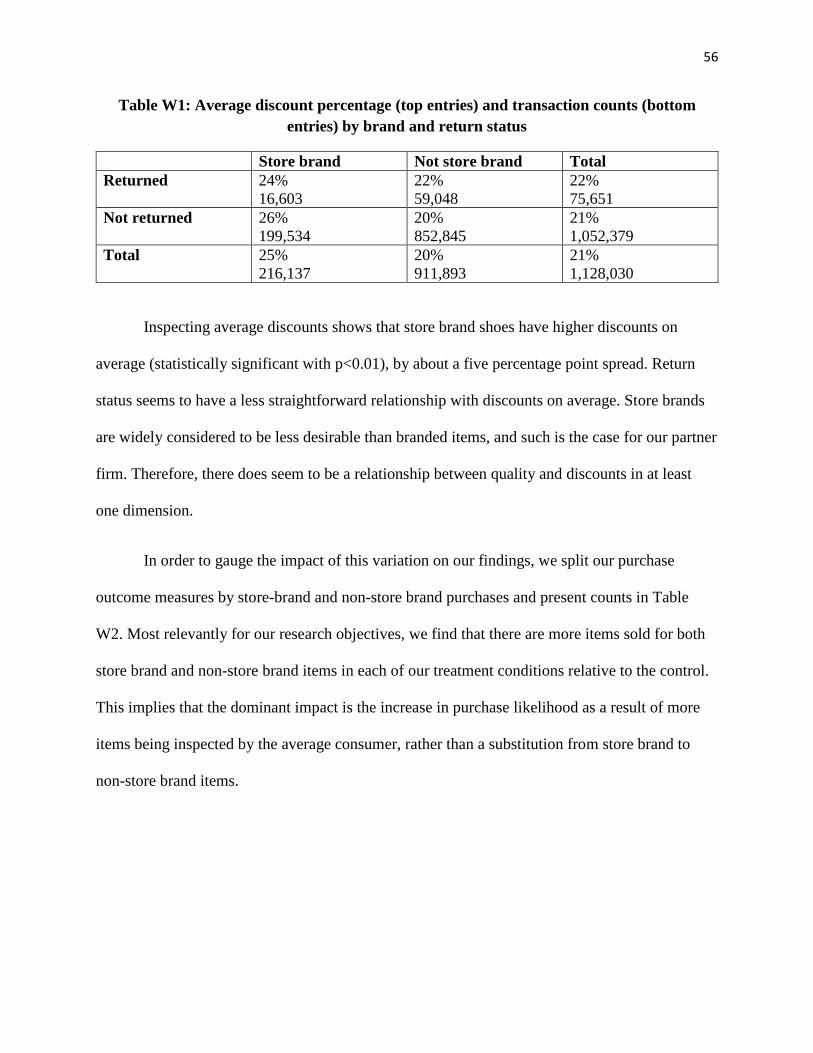
56
Table W1: Average discount percentage (top entries) and transaction counts (bottom
entries) by brand and return status
Store brand Not store brand Total
Returned 24%
16,603
22%
59,048
22%
75,651
Not returned 26%
199,534
20%
852,845
21%
1,052,379
Total 25%
216,137
20%
911,893
21%
1,128,030
Inspecting average discounts shows that store brand shoes have higher discounts on
average (statistically significant with p<0.01), by about a five percentage point spread. Return
status seems to have a less straightforward relationship with discounts on average. Store brands
are widely considered to be less desirable than branded items, and such is the case for our partner
firm. Therefore, there does seem to be a relationship between quality and discounts in at least
one dimension.
In order to gauge the impact of this variation on our findings, we split our purchase
outcome measures by store-brand and non-store brand purchases and present counts in Table
W2. Most relevantly for our research objectives, we find that there are more items sold for both
store brand and non-store brand items in each of our treatment conditions relative to the control.
This implies that the dominant impact is the increase in purchase likelihood as a result of more
items being inspected by the average consumer, rather than a substitution from store brand to
non-store brand items.
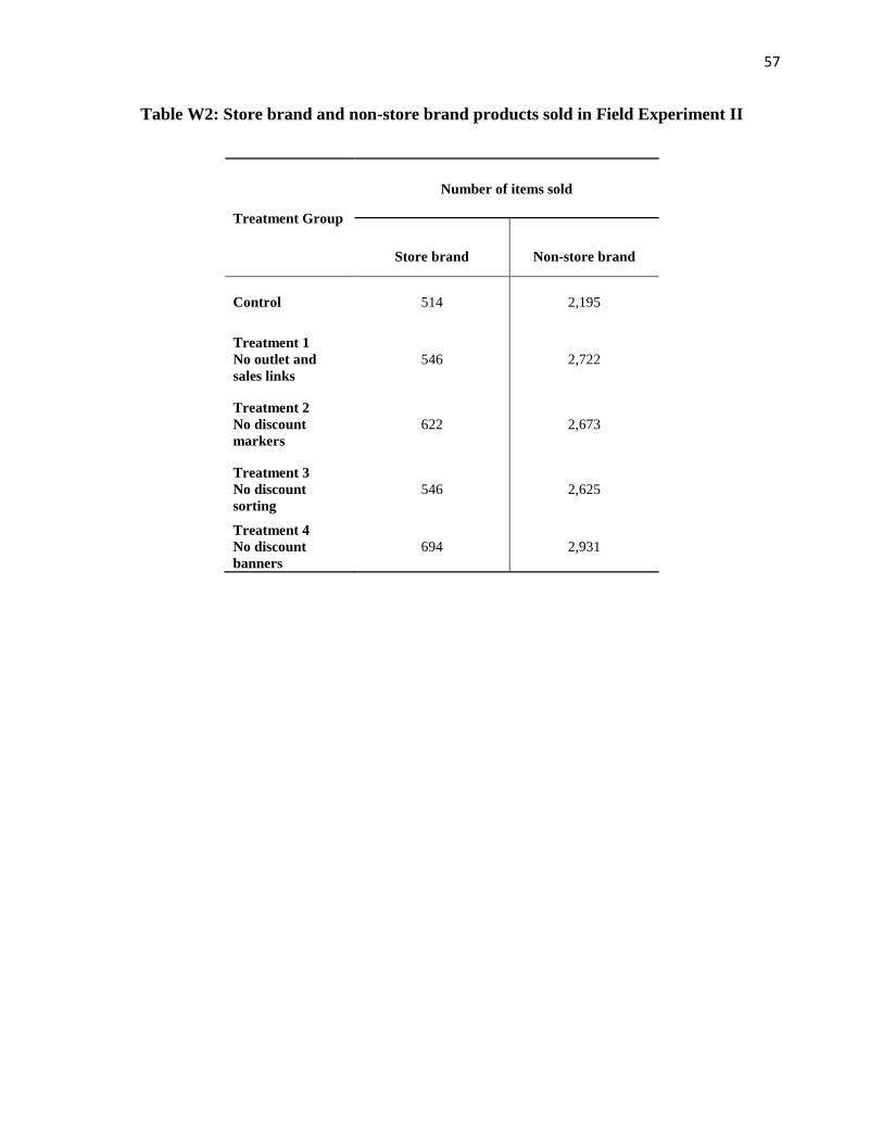
57
Table W2: Store brand and non-store brand products sold in Field Experiment II
Treatment Group
Number of items sold
Store brand Non-store brand
Control 514 2,195
Treatment 1
No outlet and
sales links
546 2,722
Treatment 2
No discount
markers
622 2,673
Treatment 3
No discount
sorting
546 2,625
Treatment 4
No discount
banners
694 2,931
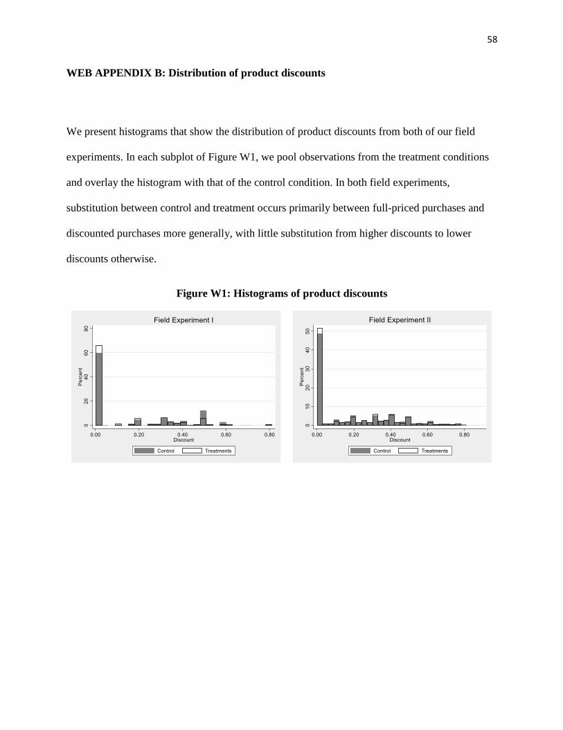
58
WEB APPENDIX B: Distribution of product discounts
We present histograms that show the distribution of product discounts from both of our field
experiments. In each subplot of Figure W1, we pool observations from the treatment conditions
and overlay the histogram with that of the control condition. In both field experiments,
substitution between control and treatment occurs primarily between full-priced purchases and
discounted purchases more generally, with little substitution from higher discounts to lower
discounts otherwise.
Figure W1: Histograms of product discounts
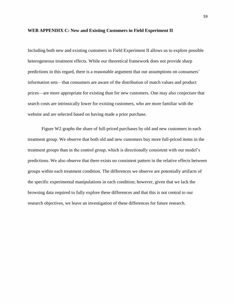
59
WEB APPENDIX C: New and Existing Customers in Field Experiment II
Including both new and existing customers in Field Experiment II allows us to explore possible
heterogeneous treatment effects. While our theoretical framework does not provide sharp
predictions in this regard, there is a reasonable argument that our assumptions on consumers’
information sets—that consumers are aware of the distribution of match values and product
prices—are more appropriate for existing than for new customers. One may also conjecture that
search costs are intrinsically lower for existing customers, who are more familiar with the
website and are selected based on having made a prior purchase.
Figure W2 graphs the share of full-priced purchases by old and new customers in each
treatment group. We observe that both old and new customers buy more full-priced items in the
treatment groups than in the control group, which is directionally consistent with our model’s
predictions. We also observe that there exists no consistent pattern in the relative effects between
groups within each treatment condition. The differences we observe are potentially artifacts of
the specific experimental manipulations in each condition; however, given that we lack the
browsing data required to fully explore these differences and that this is not central to our
research objectives, we leave an investigation of these differences for future research.
60
Figure W2: Full-priced purchases by old and new customers
61
WEB APPENDIX D: Model Analysis for Match Value Distributions beyond
𝜖𝑗~𝑖𝑖𝑑 𝑈𝑛𝑖𝑓[0,1]
In this appendix, we explore the impact of increasing search frictions on conversion and
revenue for other common match value distributions and for the case where the low-priced
product has a stochastically smaller match value than the high-priced product (i.e., is of
stochastically lower quality). We first present extensions of Theorems 1 and 2 for general match
value distributions, followed by extensive numerical simulations.
Theorem 3 (Conversion Comparison): For general match value distributions…
(i) If 𝑠 ≤ min
{∫ (𝜖𝐿 − 𝛼𝑝𝐿)𝑓𝐿(𝜖𝐿)𝑑𝜖𝐿∞
𝜖𝐿=𝛼𝑝𝐿, ∫ (𝜖𝐻 − 𝛼𝑝𝐻)𝑓𝐻(𝜖𝐻)𝑑𝜖𝐻
∞
𝜖𝐻=𝛼𝑝𝐻}, 𝑑
𝐿 = 𝑑 𝐻.
(ii) If ∫ (𝜖𝐻 − 𝛼𝑝𝐻)𝑓𝐻(𝜖𝐻)𝑑𝜖𝐻∞
𝜖𝐻=𝛼𝑝𝐻< 𝑠 ≤ ∫ (𝜖𝐿 − 𝛼𝑝𝐿)𝑓𝐿(𝜖𝐿)𝑑𝜖𝐿
∞
𝜖𝐿=𝛼𝑝𝐿, 𝑑
𝐿 < 𝑑 𝐻.
(iii) If ∫ (𝜖𝐿 − 𝛼𝑝𝐿)𝑓𝐿(𝜖𝐿)𝑑𝜖𝐿∞
𝜖𝐿=𝛼𝑝𝐿< 𝑠 ≤ ∫ (𝜖𝐻 − 𝛼𝑝𝐻)𝑓𝐻(𝜖𝐻)𝑑𝜖𝐻
∞
𝜖𝐻=𝛼𝑝𝐻, 𝑑
𝐿 > 𝑑 𝐻.
(iv) If 𝑠 > max
{∫ (𝜖𝐿 − 𝛼𝑝𝐿)𝑓𝐿(𝜖𝐿)𝑑𝜖𝐿∞
𝜖𝐿=𝛼𝑝𝐿, ∫ (𝜖𝐻 − 𝛼𝑝𝐻)𝑓𝐻(𝜖𝐻)𝑑𝜖𝐻
∞
𝜖𝐻=𝛼𝑝𝐻}, 𝑑
𝑗 ≥ 𝑑 𝑗′
iff 𝑗 = argmax𝑗={𝐿,𝐻} ∫ 𝑓𝑗(𝜖)𝑑𝜖∞
𝜖=𝛼𝑝𝑗.
Similar to Theorem 1, Theorem 3 highlights ranges for which expected conversion of a customer
who views the high-priced product first is the same, less than, or greater than expected
conversion of a customer who views the low-priced product first. As before, when the search
cost is sufficiently small, customers may search and consider both products for purchase,
regardless of if they view the high or low-priced product first. If the expected gain from
searching the low-priced product is greater than the expected gain from searching the high-priced
product – as we had when 𝜖𝑗~𝑖𝑖𝑑 𝑈𝑛𝑖𝑓[0,1] – Theorem 3(ii) shows us that for moderate search
costs, expected conversion is higher when customers view the high-priced product first,
analogous to Theorem 1(ii). In this case, the search cost is high enough to force customers who
62
view the low-priced product first to never search the high-priced product, but not too high to
prevent customers who view the high-priced product first from searching the low-priced product;
with more products to choose from, customers who view the high-priced products first are more
likely to make a purchase. If the expected gain from searching the low-priced product is less than
the expected gain from searching the high-priced product, Theorem 3(iii) shows us that for
moderate search costs, expected conversion is higher when customers view the low-priced
product first, for similar reasons as above. Finally, similar to Theorem 1(iii), Theorem 3(iv)
shows us that when the search cost is sufficiently large, the customer will never search the
second product, and conversion is greatest for whichever product is more likely to be purchased.
Theorem 4 (Revenue Comparison): For general match value distributions, if
𝑠 ≤ ∫ (𝜖𝐿 − 𝛼𝑝𝐿)𝑓𝐿(𝜖𝐿)𝑑𝜖𝐿∞
𝜖𝐿=𝛼𝑝𝐿, we have 𝑝𝐿𝑑𝐿
𝐿 + 𝑝𝐻𝑑𝐻𝐿 ≤ 𝑝𝐿𝑑𝐿
𝐻 + 𝑝𝐻𝑑𝐻𝐻.
Similar to Theorem 2(i), Theorem 4 shows us that when the search cost is sufficiently low
(corresponding to cases (i) and (ii) in Theorem 3), expected revenue is greater when customers
view the high-priced product first; intuitively, this is because expected conversion is weakly
greater for these customers.
To better understand the impact of increasing search frictions on conversion and revenue
for various match value distributions, we next present a series of simulations. For each
simulation, we randomly drew match values for the low and high-priced products for 100,000
customers. Customers in the treatment group were forced to view/consider the high-priced
product first. Unlike for the case where 𝜖𝑗~𝑖𝑖𝑑 𝑈𝑛𝑖𝑓[0,1], it may be optimal for customers in the
control group to view either the low or high-priced product first. Thus in our simulations, we
specify that customers in the control group choose to view product argmax𝑗∈{𝐿,𝐻}𝑈 𝑗 first. If
63
viewing the high-priced product first is utility maximizing, then expected conversion and
revenue are identical for customers in the treatment and control groups and increasing search
frictions would have no impact on these metrics; any differences in expected conversion and
revenue are thus attributed to the case where it is optimal for customers in the control group to
view the low-priced product first.
Figures W3-W18 show our simulation results for uniform, normal, and exponential
match value distributions, including the case where the high-priced product has a stochastically
larger match value than the low-priced product (i.e. higher price is due to expected higher
quality). Parameters of the normal and exponential match value distributions were chosen to
match the mean and variance of the standard uniform distribution used in the main body of the
paper, when possible. We can see that as the high-priced product becomes stochastically more
appealing, it is optimal for customers in the control group to view the high-priced product first
and the impact of increasing search frictions vanishes. Otherwise, we find that our results
presented in the main body of the paper are robust to common and stochastically ordered match
value distributions.
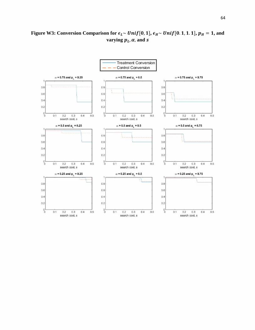
64
Figure W3: Conversion Comparison for 𝝐𝑳~ 𝑼𝒏𝒊𝒇[𝟎, 𝟏], 𝝐𝑯~ 𝑼𝒏𝒊𝒇[𝟎. 𝟏, 𝟏. 𝟏], 𝒑𝑯 = 𝟏, and
varying 𝒑𝑳, 𝜶, and 𝒔
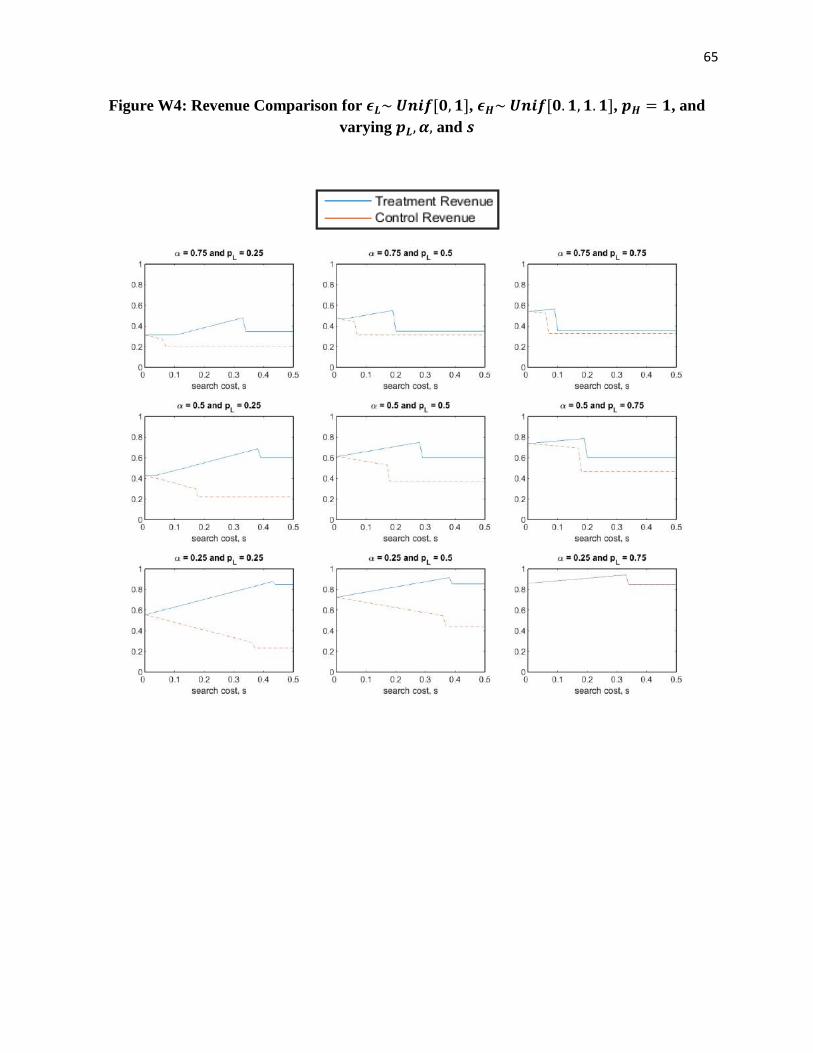
65
Figure W4: Revenue Comparison for 𝝐𝑳~ 𝑼𝒏𝒊𝒇[𝟎, 𝟏], 𝝐𝑯~ 𝑼𝒏𝒊𝒇[𝟎. 𝟏, 𝟏. 𝟏], 𝒑𝑯 = 𝟏, and
varying 𝒑𝑳, 𝜶, and 𝒔
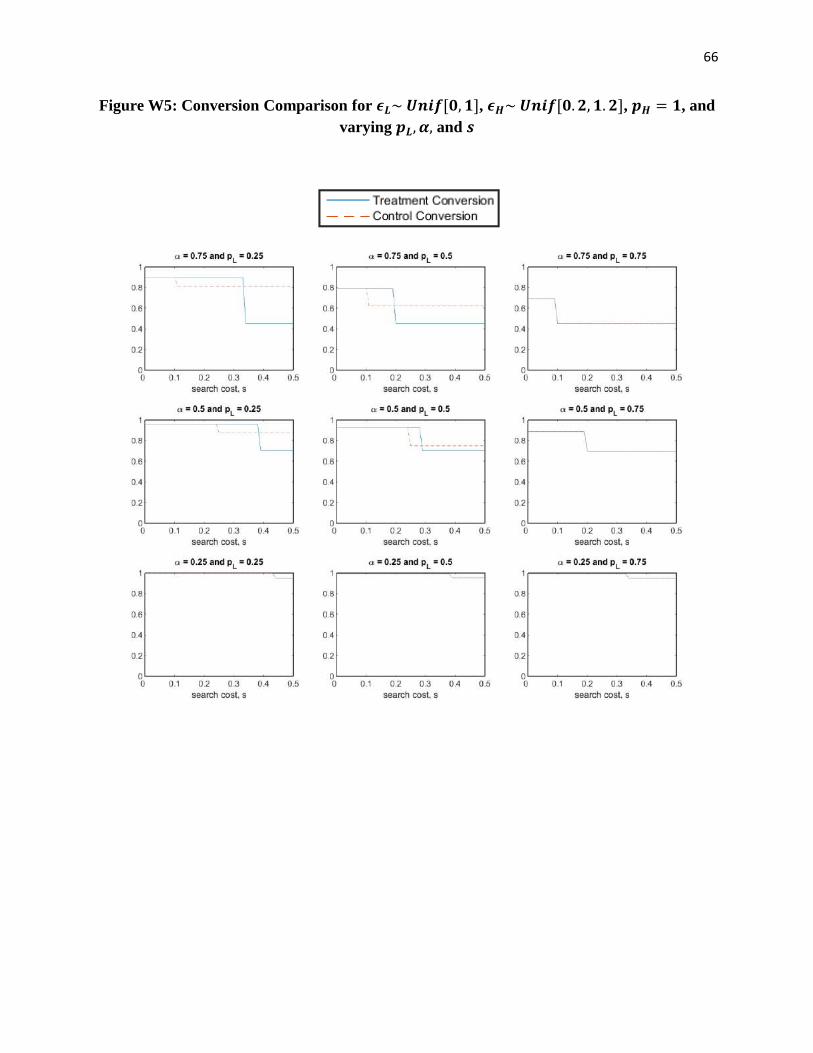
66
Figure W5: Conversion Comparison for 𝝐𝑳~ 𝑼𝒏𝒊𝒇[𝟎, 𝟏], 𝝐𝑯~ 𝑼𝒏𝒊𝒇[𝟎. 𝟐, 𝟏. 𝟐], 𝒑𝑯 = 𝟏, and
varying 𝒑𝑳, 𝜶, and 𝒔
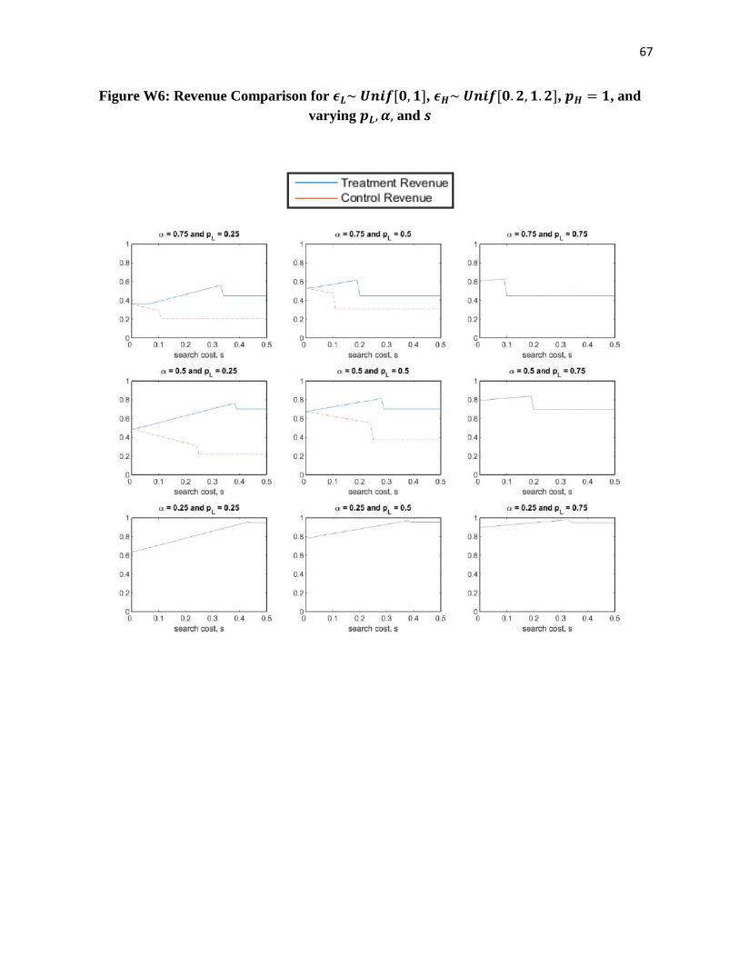
67
Figure W6: Revenue Comparison for 𝝐𝑳~ 𝑼𝒏𝒊𝒇[𝟎, 𝟏], 𝝐𝑯~ 𝑼𝒏𝒊𝒇[𝟎. 𝟐, 𝟏. 𝟐], 𝒑𝑯 = 𝟏, and
varying 𝒑𝑳, 𝜶, and 𝒔
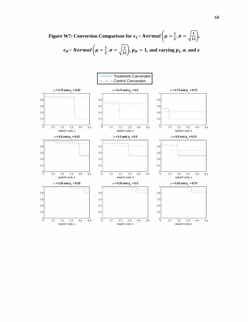
68
Figure W7: Conversion Comparison for 𝝐𝑳~ 𝑵𝒐𝒓𝒎𝒂𝒍 (𝝁 =𝟏
𝟐, 𝝈 = √
𝟏
𝟏𝟐),
𝝐𝑯~ 𝑵𝒐𝒓𝒎𝒂𝒍 (𝝁 =𝟏
𝟐, 𝝈 = √
𝟏
𝟏𝟐), 𝒑𝑯 = 𝟏, and varying 𝒑𝑳, 𝜶, and 𝒔
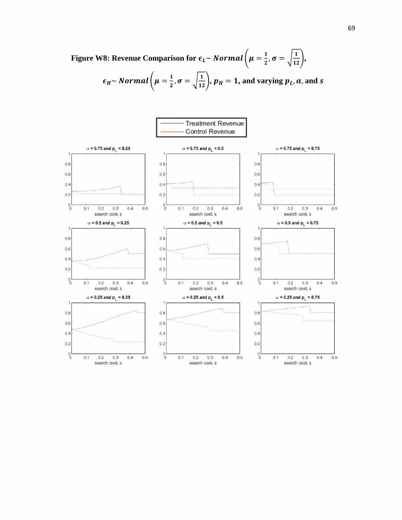
69
Figure W8: Revenue Comparison for 𝝐𝑳~ 𝑵𝒐𝒓𝒎𝒂𝒍 (𝝁 =𝟏
𝟐, 𝝈 = √
𝟏
𝟏𝟐),
𝝐𝑯~ 𝑵𝒐𝒓𝒎𝒂𝒍 (𝝁 =𝟏
𝟐, 𝝈 = √
𝟏
𝟏𝟐), 𝒑𝑯 = 𝟏, and varying 𝒑𝑳, 𝜶, and 𝒔
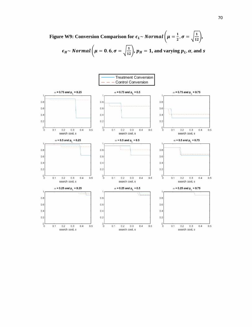
70
Figure W9: Conversion Comparison for 𝝐𝑳~ 𝑵𝒐𝒓𝒎𝒂𝒍 (𝝁 =𝟏
𝟐, 𝝈 = √
𝟏
𝟏𝟐),
𝝐𝑯~ 𝑵𝒐𝒓𝒎𝒂𝒍 (𝝁 = 𝟎. 𝟔, 𝝈 = √𝟏
𝟏𝟐), 𝒑𝑯 = 𝟏, and varying 𝒑𝑳, 𝜶, and 𝒔
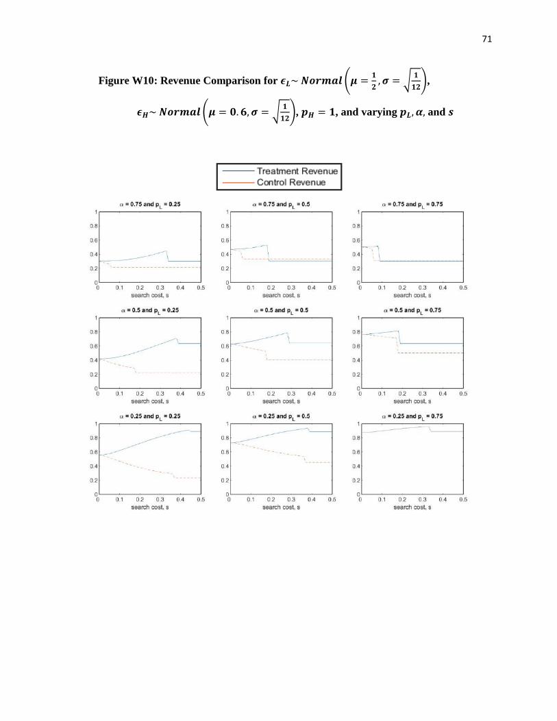
71
Figure W10: Revenue Comparison for 𝝐𝑳~ 𝑵𝒐𝒓𝒎𝒂𝒍 (𝝁 =𝟏
𝟐, 𝝈 = √
𝟏
𝟏𝟐),
𝝐𝑯~ 𝑵𝒐𝒓𝒎𝒂𝒍 (𝝁 = 𝟎. 𝟔, 𝝈 = √𝟏
𝟏𝟐), 𝒑𝑯 = 𝟏, and varying 𝒑𝑳, 𝜶, and 𝒔
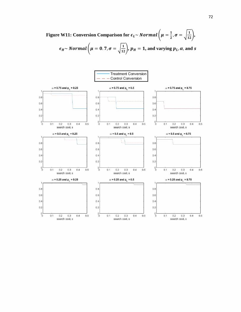
72
Figure W11: Conversion Comparison for 𝝐𝑳~ 𝑵𝒐𝒓𝒎𝒂𝒍 (𝝁 =𝟏
𝟐, 𝝈 = √
𝟏
𝟏𝟐),
𝝐𝑯~ 𝑵𝒐𝒓𝒎𝒂𝒍 (𝝁 = 𝟎. 𝟕, 𝝈 = √𝟏
𝟏𝟐), 𝒑𝑯 = 𝟏, and varying 𝒑𝑳, 𝜶, and 𝒔
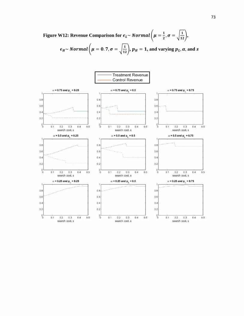
73
Figure W12: Revenue Comparison for 𝝐𝑳~ 𝑵𝒐𝒓𝒎𝒂𝒍 (𝝁 =𝟏
𝟐, 𝝈 = √
𝟏
𝟏𝟐),
𝝐𝑯~ 𝑵𝒐𝒓𝒎𝒂𝒍 (𝝁 = 𝟎. 𝟕, 𝝈 = √𝟏
𝟏𝟐), 𝒑𝑯 = 𝟏, and varying 𝒑𝑳, 𝜶, and 𝒔
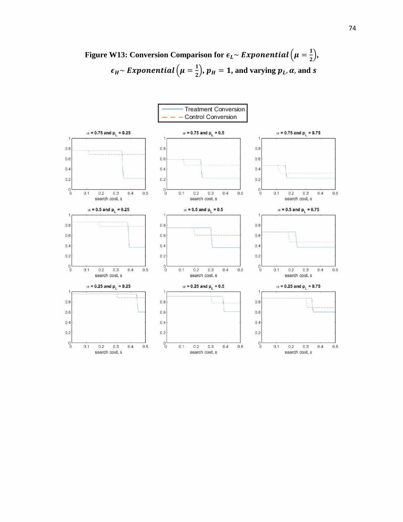
74
Figure W13: Conversion Comparison for 𝝐𝑳~ 𝑬𝒙𝒑𝒐𝒏𝒆𝒏𝒕𝒊𝒂𝒍 (𝝁 =𝟏
𝟐),
𝝐𝑯~ 𝑬𝒙𝒑𝒐𝒏𝒆𝒏𝒕𝒊𝒂𝒍 (𝝁 =𝟏
𝟐), 𝒑𝑯 = 𝟏, and varying 𝒑𝑳, 𝜶, and 𝒔
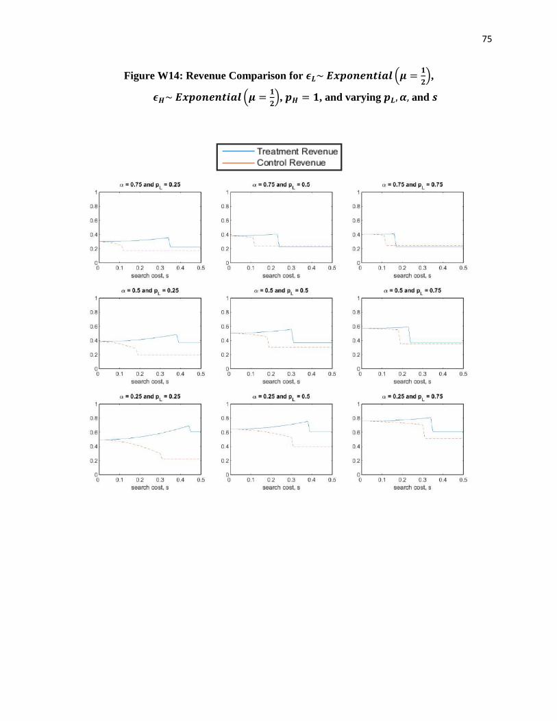
75
Figure W14: Revenue Comparison for 𝝐𝑳~ 𝑬𝒙𝒑𝒐𝒏𝒆𝒏𝒕𝒊𝒂𝒍 (𝝁 =𝟏
𝟐),
𝝐𝑯~ 𝑬𝒙𝒑𝒐𝒏𝒆𝒏𝒕𝒊𝒂𝒍 (𝝁 =𝟏
𝟐), 𝒑𝑯 = 𝟏, and varying 𝒑𝑳, 𝜶, and 𝒔
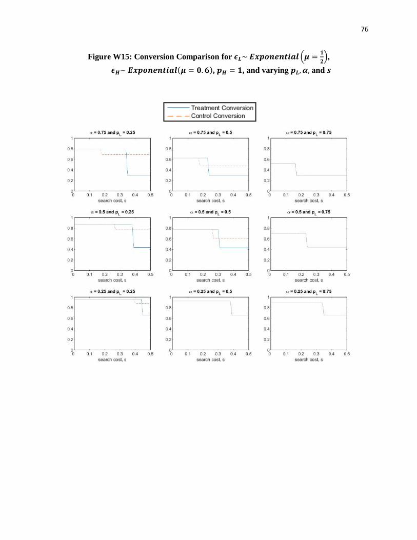
76
Figure W15: Conversion Comparison for 𝝐𝑳~ 𝑬𝒙𝒑𝒐𝒏𝒆𝒏𝒕𝒊𝒂𝒍 (𝝁 =𝟏
𝟐),
𝝐𝑯~ 𝑬𝒙𝒑𝒐𝒏𝒆𝒏𝒕𝒊𝒂𝒍(𝝁 = 𝟎. 𝟔), 𝒑𝑯 = 𝟏, and varying 𝒑𝑳, 𝜶, and 𝒔
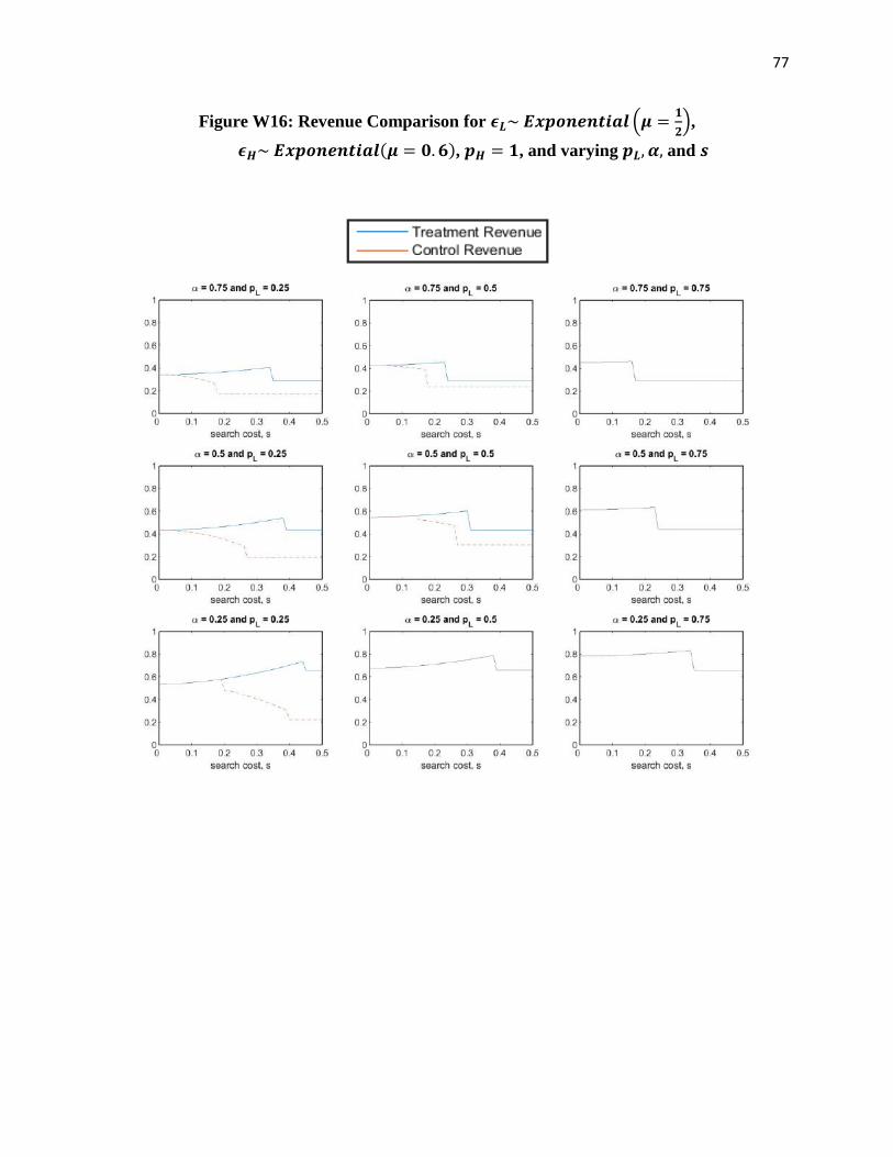
77
Figure W16: Revenue Comparison for 𝝐𝑳~ 𝑬𝒙𝒑𝒐𝒏𝒆𝒏𝒕𝒊𝒂𝒍 (𝝁 =𝟏
𝟐),
𝝐𝑯~ 𝑬𝒙𝒑𝒐𝒏𝒆𝒏𝒕𝒊𝒂𝒍(𝝁 = 𝟎. 𝟔), 𝒑𝑯 = 𝟏, and varying 𝒑𝑳, 𝜶, and 𝒔
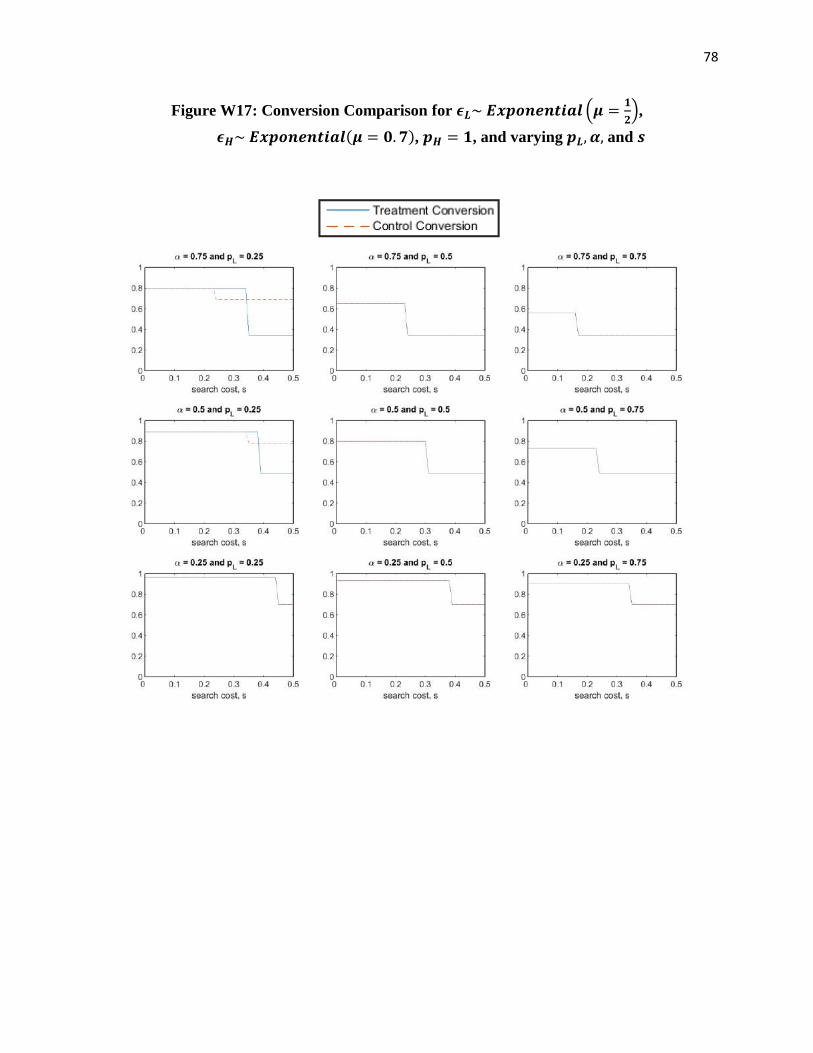
78
Figure W17: Conversion Comparison for 𝝐𝑳~ 𝑬𝒙𝒑𝒐𝒏𝒆𝒏𝒕𝒊𝒂𝒍 (𝝁 =𝟏
𝟐),
𝝐𝑯~ 𝑬𝒙𝒑𝒐𝒏𝒆𝒏𝒕𝒊𝒂𝒍(𝝁 = 𝟎. 𝟕), 𝒑𝑯 = 𝟏, and varying 𝒑𝑳, 𝜶, and 𝒔
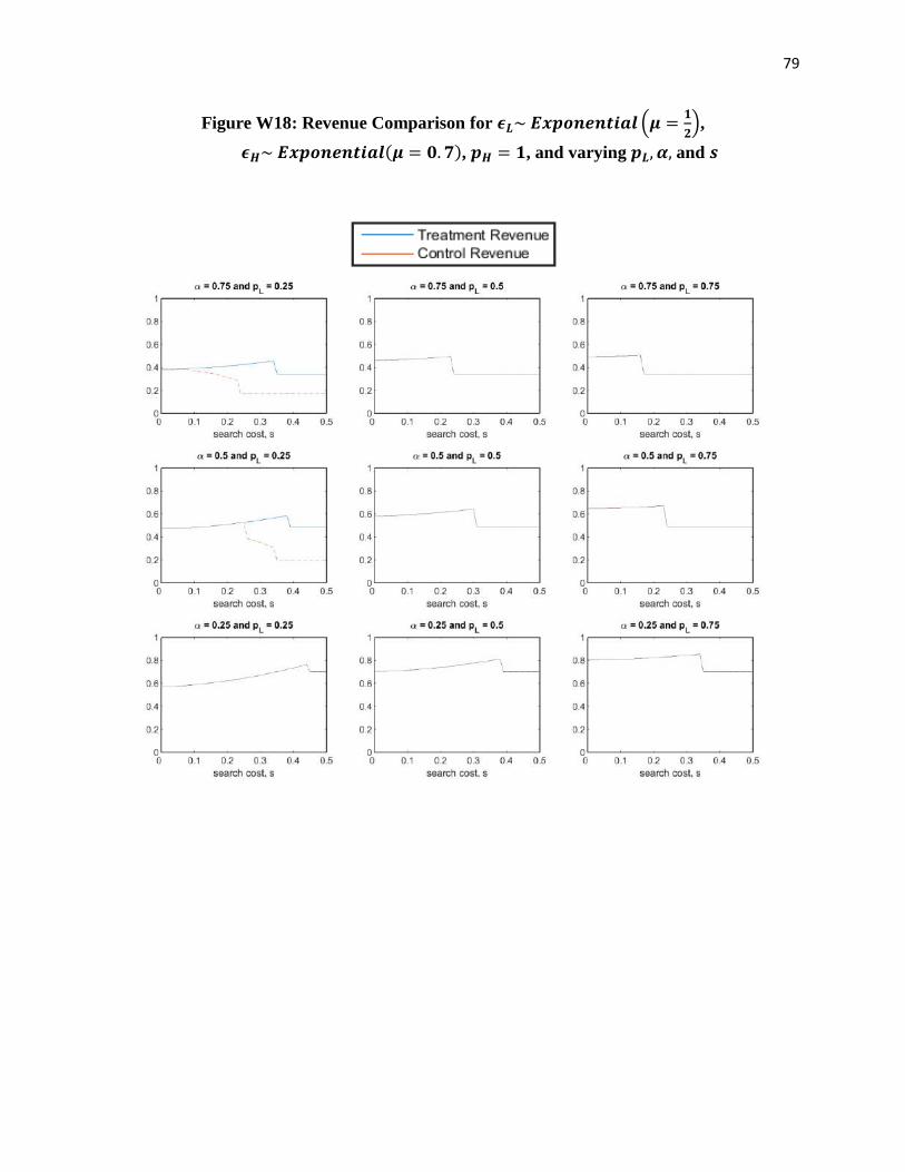
79
Figure W18: Revenue Comparison for 𝝐𝑳~ 𝑬𝒙𝒑𝒐𝒏𝒆𝒏𝒕𝒊𝒂𝒍 (𝝁 =𝟏
𝟐),
𝝐𝑯~ 𝑬𝒙𝒑𝒐𝒏𝒆𝒏𝒕𝒊𝒂𝒍(𝝁 = 𝟎. 𝟕), 𝒑𝑯 = 𝟏, and varying 𝒑𝑳, 𝜶, and 𝒔
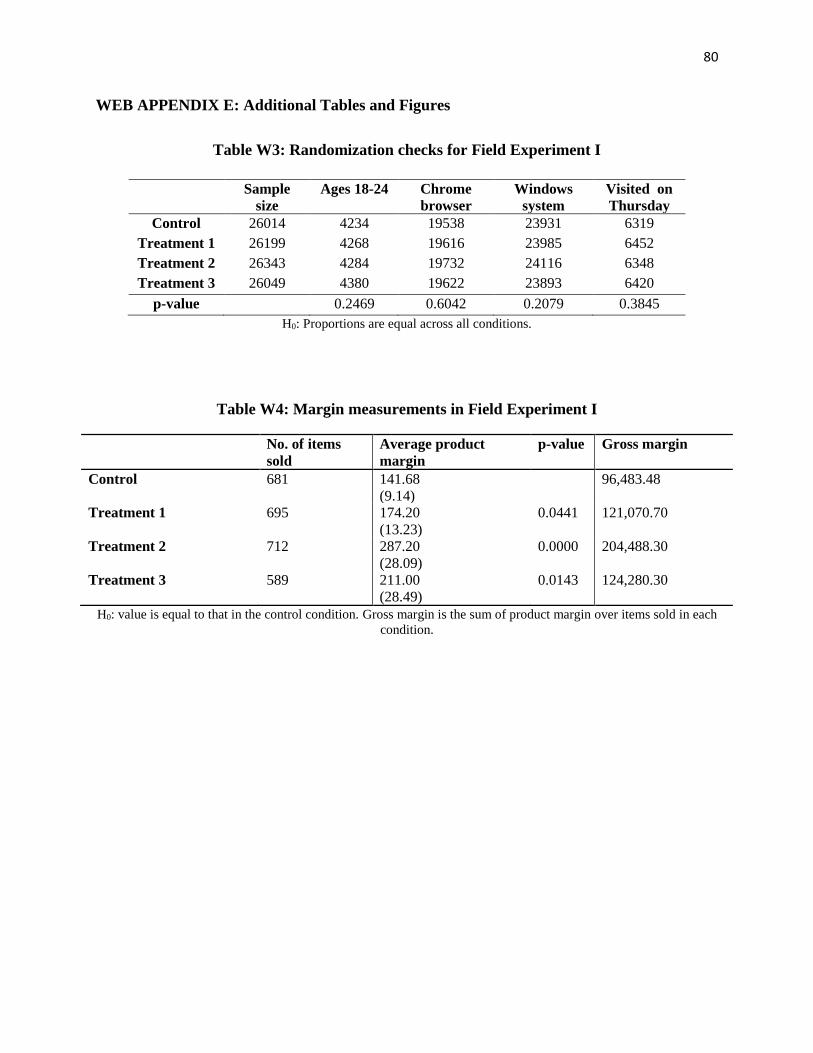
80
WEB APPENDIX E: Additional Tables and Figures
Table W3: Randomization checks for Field Experiment I
Sample
size
Ages 18-24 Chrome
browser
Windows
system
Visited on
Thursday
Control 26014 4234 19538 23931 6319
Treatment 1 26199 4268 19616 23985 6452
Treatment 2 26343 4284 19732 24116 6348
Treatment 3 26049 4380 19622 23893 6420
p-value
0.2469 0.6042 0.2079 0.3845
H0: Proportions are equal across all conditions.
Table W4: Margin measurements in Field Experiment I
No. of items
sold
Average product
margin
p-value Gross margin
Control 681 141.68
(9.14)
96,483.48
Treatment 1 695 174.20
(13.23)
0.0441 121,070.70
Treatment 2 712 287.20
(28.09)
0.0000 204,488.30
Treatment 3 589 211.00
(28.49)
0.0143 124,280.30
H0: value is equal to that in the control condition. Gross margin is the sum of product margin over items sold in each
condition.
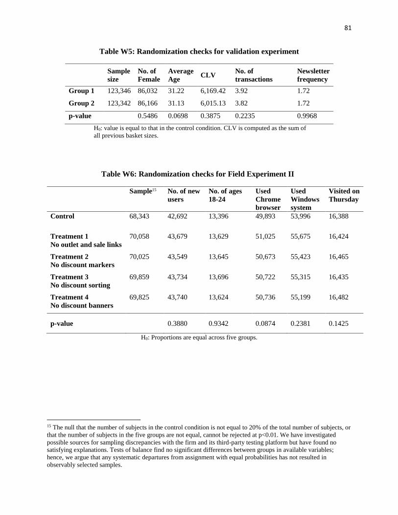
81
Table W5: Randomization checks for validation experiment
Sample
size
No. of
Female
Average
Age CLV
No. of
transactions
Newsletter
frequency
Group 1 123,346 86,032 31.22 6,169.42 3.92 1.72
Group 2 123,342 86,166 31.13 6,015.13 3.82 1.72
p-value
0.5486 0.0698 0.3875 0.2235 0.9968
H0: value is equal to that in the control condition. CLV is computed as the sum of
all previous basket sizes.
Table W6: Randomization checks for Field Experiment II
Sample15 No. of new
users
No. of ages
18-24
Used
Chrome
browser
Used
Windows
system
Visited on
Thursday
Control 68,343 42,692 13,396 49,893 53,996 16,388
Treatment 1
No outlet and sale links
70,058 43,679 13,629 51,025 55,675 16,424
Treatment 2
No discount markers
70,025 43,549 13,645 50,673 55,423 16,465
Treatment 3
No discount sorting
69,859 43,734 13,696 50,722 55,315 16,435
Treatment 4
No discount banners
69,825 43,740 13,624 50,736 55,199 16,482
p-value 0.3880 0.9342 0.0874 0.2381 0.1425
H0: Proportions are equal across five groups.
15 The null that the number of subjects in the control condition is not equal to 20% of the total number of subjects, or
that the number of subjects in the five groups are not equal, cannot be rejected at p<0.01. We have investigated
possible sources for sampling discrepancies with the firm and its third-party testing platform but have found no
satisfying explanations. Tests of balance find no significant differences between groups in available variables;
hence, we argue that any systematic departures from assignment with equal probabilities has not resulted in
observably selected samples.
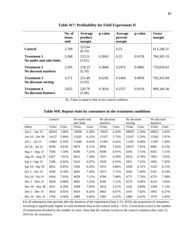
82
Table W7: Profitability for Field Experiment II
No. of
items
sold
Average
product
margin
p-value Average
percent
margin
p-value Gross
margin
Control 2,709 225.64
(6.33) 0.23 611,246.31
Treatment 1
No outlet and sales links
3,268 215.51
(5.01)
0.2043 0.25 0.0159 704,302.19
Treatment 2
No discount markers
3,295 218.23
(5.70)
0.3840 0.2472 0.0883 719,059.63
Treatment 3
No discount sorting
3,171 221.49
(5.65)
0.6245 0.2464 0.0959 702,355.94
Treatment 4
No discount banners
3,625 220.78
(5.46)
0.5616 0.2527 0.0119 800,344.38
H0: Value is equal to that in the control condition.
Table W8: Repeat visits by consumers in the treatment conditions
Control No outlet and
sale links
No discount
markers
No discount
sorting
No discount
banners
Dates Visits Conv Visits Conv Visits Conv Visits Conv Visits Conv
Jun 1 - Jun 15 68343 1.98% 70058 2.28% 70025 2.29% 69859 2.30% 69825 2.45%
Jun 16 - Jun 30 14157 5.88% 15205 6.15% 15337 5.73% 15167 5.70% 15302 7.07%
Jul 1 - Jul 15 10461 6.10% 11649 6.03% 11393 6.42% 11281 6.60% 11497 7.44%
Jul 16 - Jul 31 9058 9.03% 9870 8.11% 9956 7.63% 10037 7.91% 9962 9.13%
Aug 1 - Aug 15 7560 7.34% 8290 7.25% 8308 6.91% 8295 7.15% 8501 7.15%
Aug 16 - Aug 31 6367 7.81% 6815 7.18% 7025 6.28% 6918 6.79% 7091 7.63%
Sep 1 - Sep 15 5288 6.92% 5635 6.87% 5928 6.55% 5921 7.52% 5905 7.50%
Sep 16 - Sep 30 4922 6.85% 5306 6.20% 5553 6.86% 5569 6.12% 5520 8.13%
Oct 1 - Oct 15 4549 6.70% 4945 7.46% 5073 7.71% 5045 7.49% 5101 8.10%
Oct 16 - Oct 31 4364 7.03% 4658 7.11% 4784 7.48% 4771 7.76% 4755 7.38%
Nov 1 - Nov 15 3824 6.88% 4065 7.23% 4186 7.12% 4275 5.89% 4253 7.05%
Nov 16 - Nov 30 2931 6.28% 3308 7.04% 3414 5.27% 3342 5.69% 3294 7.13%
Dec 1 - Dec 15 3654 8.95% 4019 8.43% 4002 8.67% 4191 7.92% 3992 8.37%
Dec 16 - Dec 31 1764 6.58% 1889 5.93% 1985 6.25% 1980 6.92% 1970 5.43%
For all subsequent time periods after the duration of the experiment (June 1-15, 2016), the proportion of consumers
revisiting is significantly higher in each treatment than in the control with p < 0.01. Conversion (conv) is the number
of transactions divided by the number of visits. Note that the website reverts to the control condition after June 15,
2016 for all consumers.
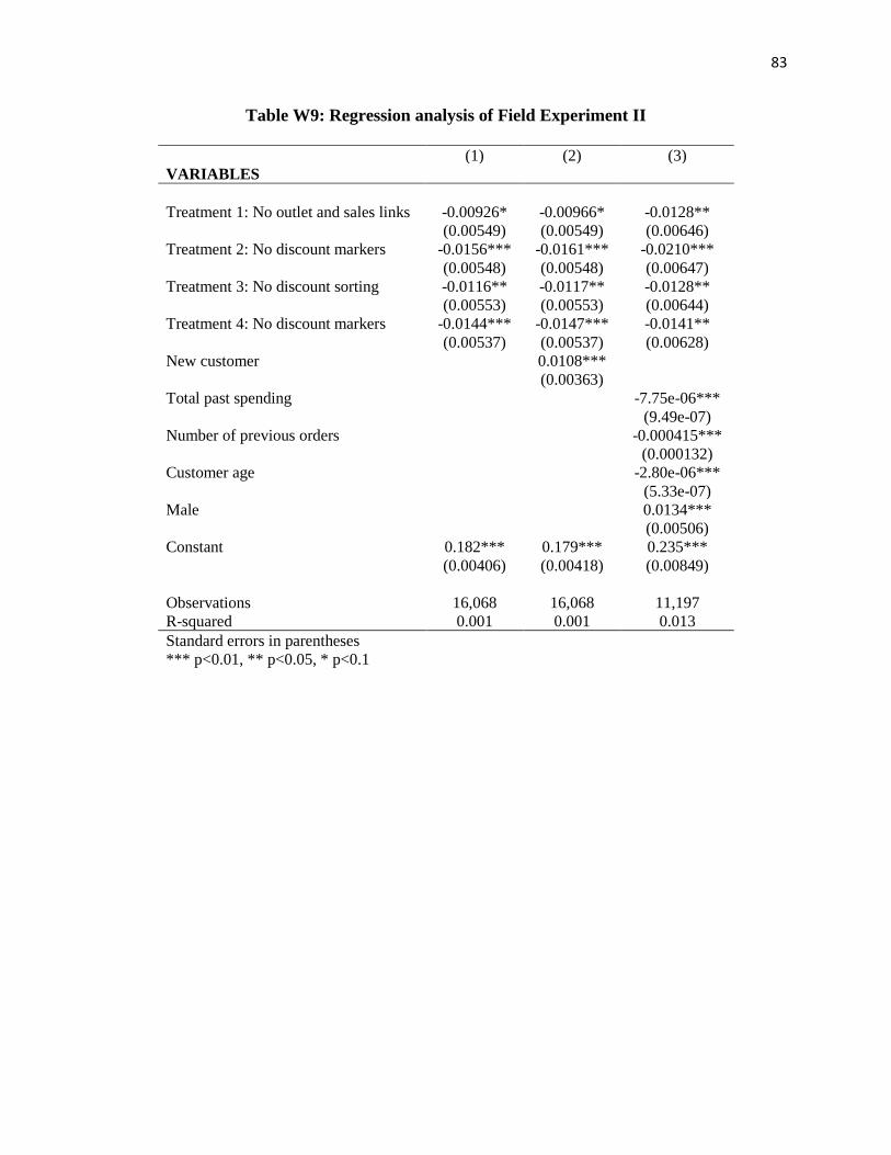
83
Table W9: Regression analysis of Field Experiment II
(1) (2) (3)
VARIABLES
Treatment 1: No outlet and sales links -0.00926* -0.00966* -0.0128**
(0.00549) (0.00549) (0.00646)
Treatment 2: No discount markers -0.0156*** -0.0161*** -0.0210***
(0.00548) (0.00548) (0.00647)
Treatment 3: No discount sorting -0.0116** -0.0117** -0.0128**
(0.00553) (0.00553) (0.00644)
Treatment 4: No discount markers -0.0144*** -0.0147*** -0.0141**
(0.00537) (0.00537) (0.00628)
New customer 0.0108***
(0.00363) Total past spending -7.75e-06***
(9.49e-07)
Number of previous orders -0.000415***
(0.000132)
Customer age -2.80e-06***
(5.33e-07)
Male 0.0134***
(0.00506)
Constant 0.182*** 0.179*** 0.235***
(0.00406) (0.00418) (0.00849)
Observations 16,068 16,068 11,197
R-squared 0.001 0.001 0.013
Standard errors in parentheses
*** p<0.01, ** p<0.05, * p<0.1
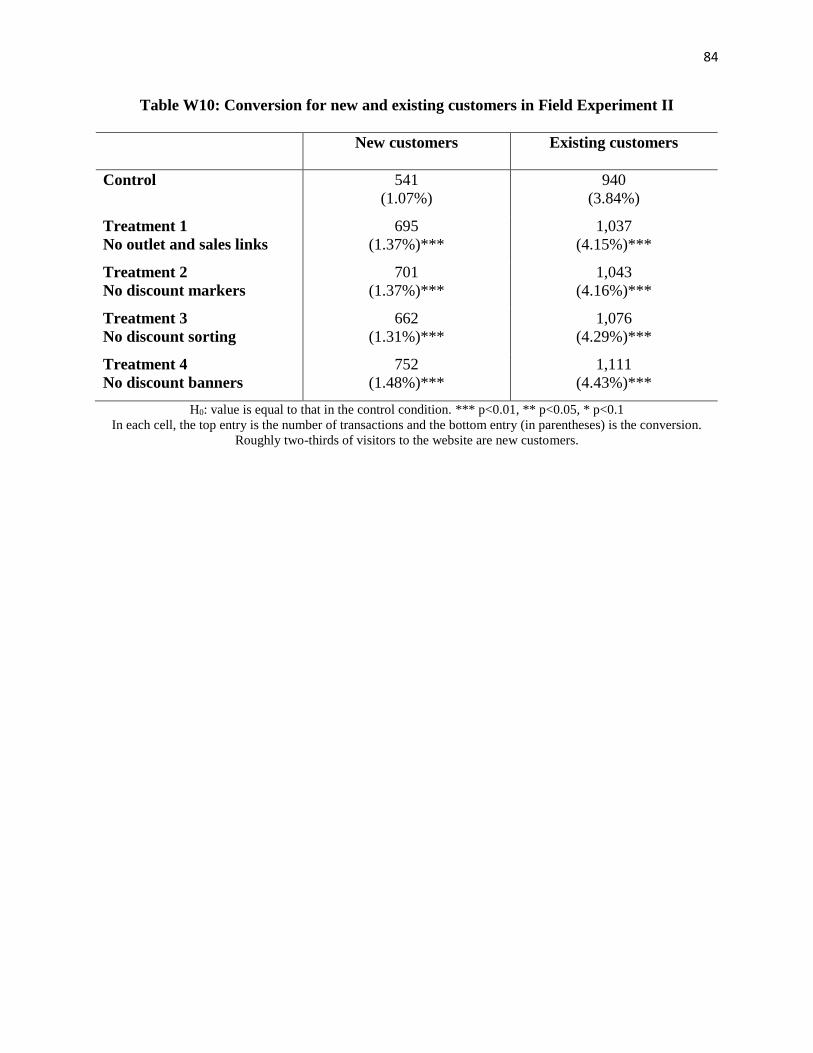
84
Table W10: Conversion for new and existing customers in Field Experiment II
New customers Existing customers
Control
541
(1.07%)
940
(3.84%)
Treatment 1
No outlet and sales links
695
(1.37%)***
1,037
(4.15%)***
Treatment 2
No discount markers
701
(1.37%)***
1,043
(4.16%)***
Treatment 3
No discount sorting
662
(1.31%)***
1,076
(4.29%)***
Treatment 4
No discount banners
752
(1.48%)***
1,111
(4.43%)***
H0: value is equal to that in the control condition. *** p<0.01, ** p<0.05, * p<0.1
In each cell, the top entry is the number of transactions and the bottom entry (in parentheses) is the conversion.
Roughly two-thirds of visitors to the website are new customers.
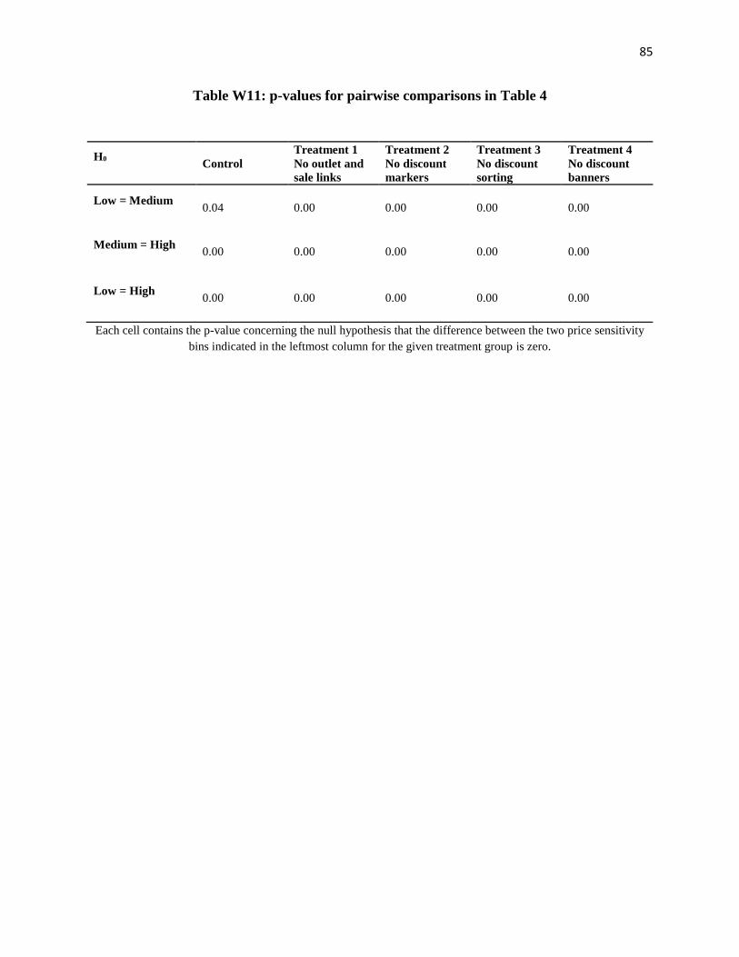
85
Table W11: p-values for pairwise comparisons in Table 4
Each cell contains the p-value concerning the null hypothesis that the difference between the two price sensitivity
bins indicated in the leftmost column for the given treatment group is zero.
H0 Control
Treatment 1
No outlet and
sale links
Treatment 2
No discount
markers
Treatment 3
No discount
sorting
Treatment 4
No discount
banners
Low = Medium 0.04 0.00 0.00 0.00 0.00
Medium = High 0.00 0.00 0.00 0.00 0.00
Low = High 0.00 0.00 0.00 0.00 0.00
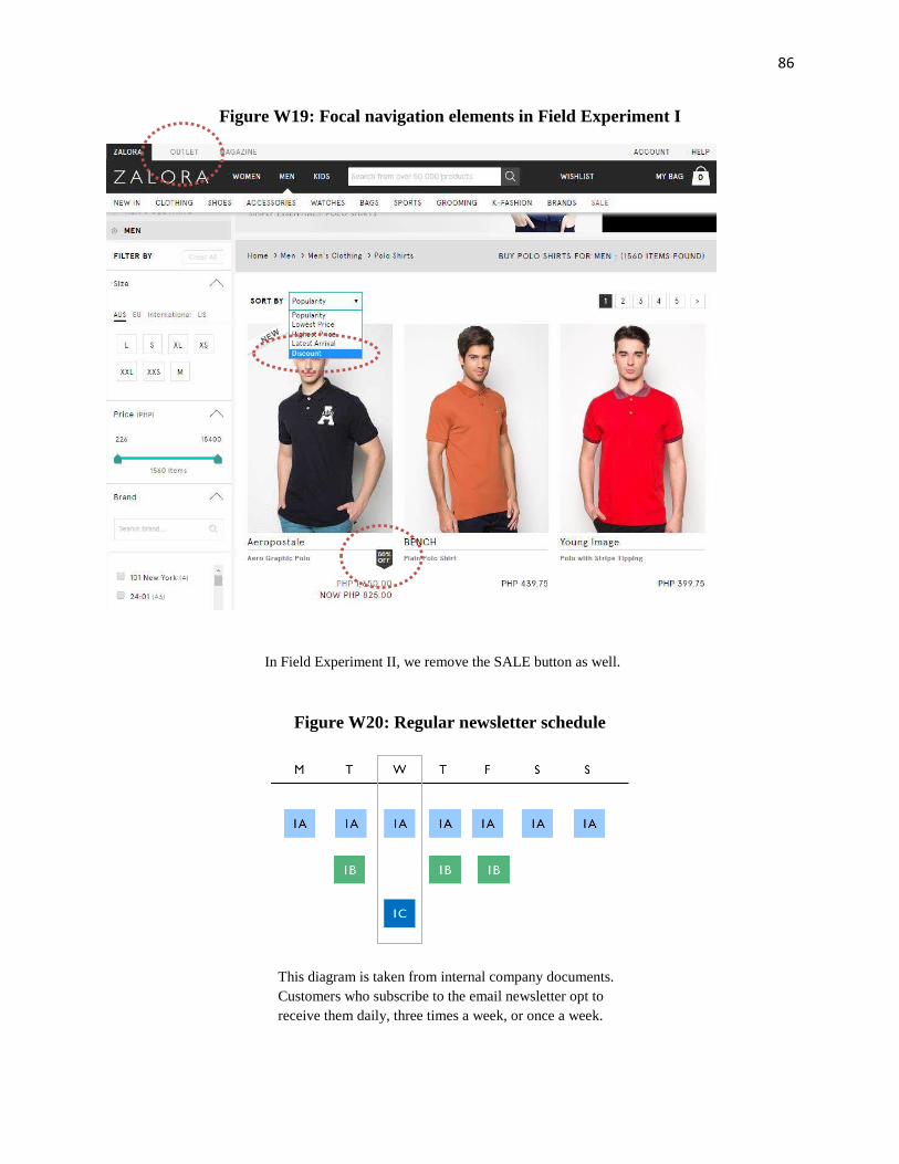
86
Figure W19: Focal navigation elements in Field Experiment I
In Field Experiment II, we remove the SALE button as well.
Figure W20: Regular newsletter schedule
This diagram is taken from internal company documents.
Customers who subscribe to the email newsletter opt to
receive them daily, three times a week, or once a week.

87
Figure W21: Examples of discount and non-discount email newsletters
This pair of newsletters is representative of the array of discount- and non-discount
newsletters sent out in the validation experiment. Product categories differed
between days, as did newsletters sent to male and female recipients. These are two
out of a total of 22 unique newsletters sent out during the experiment.

88
Figure W22: Examples of discount banners

89
WEB APPENDIX F: Proofs
Proof of Lemma 1
Recall that xj = εj′ − αpj′ + αpj such that
∫ ∞εj=εj′−αpj′+αpj
(εj − αpj − εj′ + αpj′)fj(εj)dεj = s.
As is common in the search literature, we define xj − αpj to be the reservation utility for product
j; the consumer will search product j if and only if εj′ − αpj′ < xj − αpj . For εj ∼iid Unif [0, 1],
it can be shown that xL = xH = 1−√2s.
We prove Lemma 1 separately for different ranges of the search cost, s, which dictate the
consumer’s search behavior. Note that a customer has a positive probability of searching product
j only if her expected benefit of searching j exceeds her search cost s, i.e. if
s ≤∫ 1
εj=0
max{0, εj − αpj}dεj =∫ 1
εj=αpj
(εj − αpj)dεj =1
2(1− αpj)2.
Furthermore, if the customer views product H first, she will always choose to incur the search
cost s to view product L if the search cost is sufficiently small, specifically, if
P (εH > x− αpL + αpH) = 0 which occurs when x ≤ 1 + αpL − αpH (equivalently,
s ≤ 12(αpH − αpL)2).
Although 12(αpH − αpL)2 ≤ 1
2(1− αpL)2, we may have 1
2(αpH − αpL)2 ≤ 1
2(1− αpH)2 or
12(αpH − αpL)2 ≥ 1
2(1− αpH)2. Each of these two scenarios leads to four regions on the
continuum of possible search costs. Figure WF.1 illustrates these regions and maps them to cases
in the proof that follows.
Case (a): s ≤ min{12(1− αpH)2, 12(αpH − αpL)
2}
In this case, the search cost is small enough such that after viewing the first product j, the
customer will choose to incur the search cost to search product j′ 6= j with positive probability.

90
Figure WF.1: Possible regions of search costs as a function of parameters.
When the customer views the high-priced product first (j = H), the condition
s ≤ 12(αpH − αpL)2 tells us that the customer will always choose to incur the search cost to
search product L, regardless of her realization of εH . In such case, we have
E[UH ] = E[εL − αpL|εL − αpL ≥ max{0, εH − αpH}]P (εL − αpL ≥ max{0, εH − αpH})
+ E[εH − αpH |εH − αpH ≥ max{0, εL − αpL}]P (εH − αpH ≥ max{0, εL − αpL})− s.
(1)
We next present expressions for each of the terms above.
E[εL − αpL|εL − αpL ≥ max{0, εH − αpH}]P (εL − αpL ≥ max{0, εH − αpH})
=
∫ 1
εL=1−αpH+αpL
∫ 1
εH=0
(εL − αpL)dεHdεL +
∫ 1−αpH+αpL
εL=αpL
∫ εL−αpL+αpH
εH=0
(εL − αpL)dεHdεL
=1
3− αpL +
1
2αpH +
1
2(αpL)
2 − 1
2(αpH)
2 +1
6(αpH)
3
(2)
E[εH − αpH |εH − αpH ≥ max{0, εL − αpL}]P (εH − αpH ≥ max{0, εL − αpL})
=
∫ 1
εH=αpH
∫ εH−αpH+αpL
εL=0
(εH − αpH)dεLdεH
=1
3− αpH +
1
2αpL + (αpH)
2 − αpLαpH −1
3(αpH)
3 +1
2αpL(αpH)
2
(3)
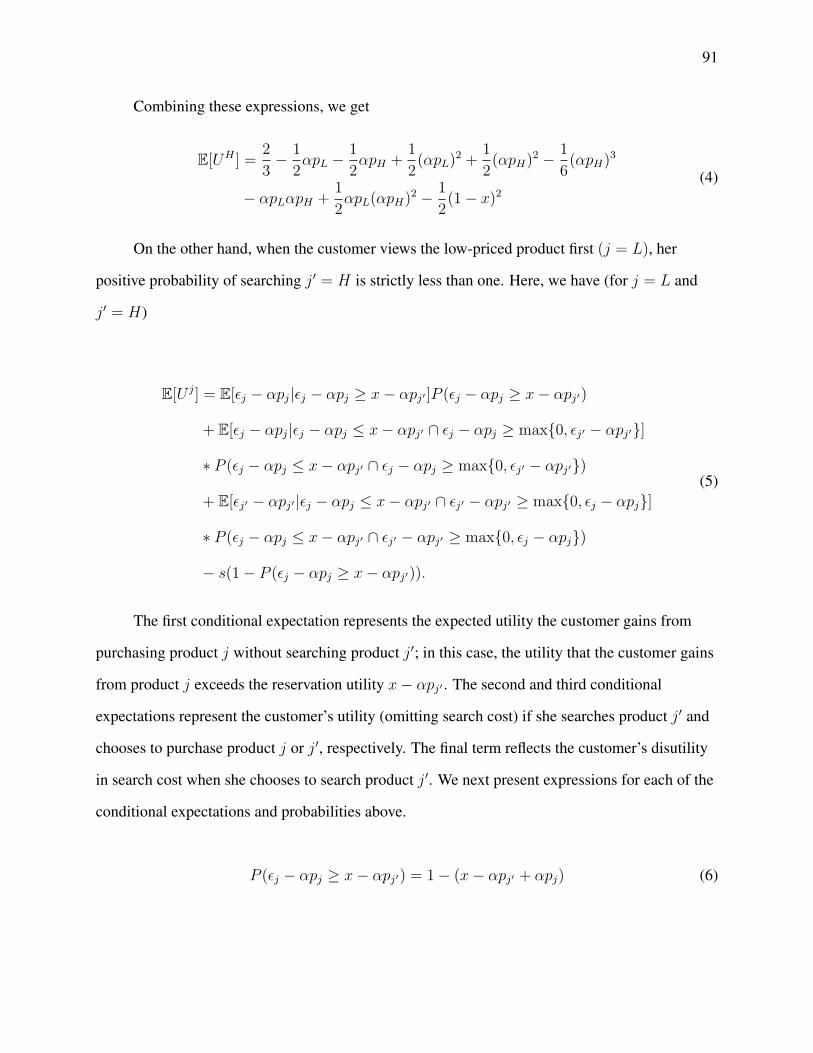
91
Combining these expressions, we get
E[UH ] =2
3− 1
2αpL −
1
2αpH +
1
2(αpL)
2 +1
2(αpH)
2 − 1
6(αpH)
3
− αpLαpH +1
2αpL(αpH)
2 − 1
2(1− x)2
(4)
On the other hand, when the customer views the low-priced product first (j = L), her
positive probability of searching j′ = H is strictly less than one. Here, we have (for j = L and
j′ = H)
E[U j] = E[εj − αpj|εj − αpj ≥ x− αpj′ ]P (εj − αpj ≥ x− αpj′)
+ E[εj − αpj|εj − αpj ≤ x− αpj′ ∩ εj − αpj ≥ max{0, εj′ − αpj′}]
∗ P (εj − αpj ≤ x− αpj′ ∩ εj − αpj ≥ max{0, εj′ − αpj′})
+ E[εj′ − αpj′ |εj − αpj ≤ x− αpj′ ∩ εj′ − αpj′ ≥ max{0, εj − αpj}]
∗ P (εj − αpj ≤ x− αpj′ ∩ εj′ − αpj′ ≥ max{0, εj − αpj})
− s(1− P (εj − αpj ≥ x− αpj′)).
(5)
The first conditional expectation represents the expected utility the customer gains from
purchasing product j without searching product j′; in this case, the utility that the customer gains
from product j exceeds the reservation utility x− αpj′ . The second and third conditional
expectations represent the customer’s utility (omitting search cost) if she searches product j′ and
chooses to purchase product j or j′, respectively. The final term reflects the customer’s disutility
in search cost when she chooses to search product j′. We next present expressions for each of the
conditional expectations and probabilities above.
P (εj − αpj ≥ x− αpj′) = 1− (x− αpj′ + αpj) (6)
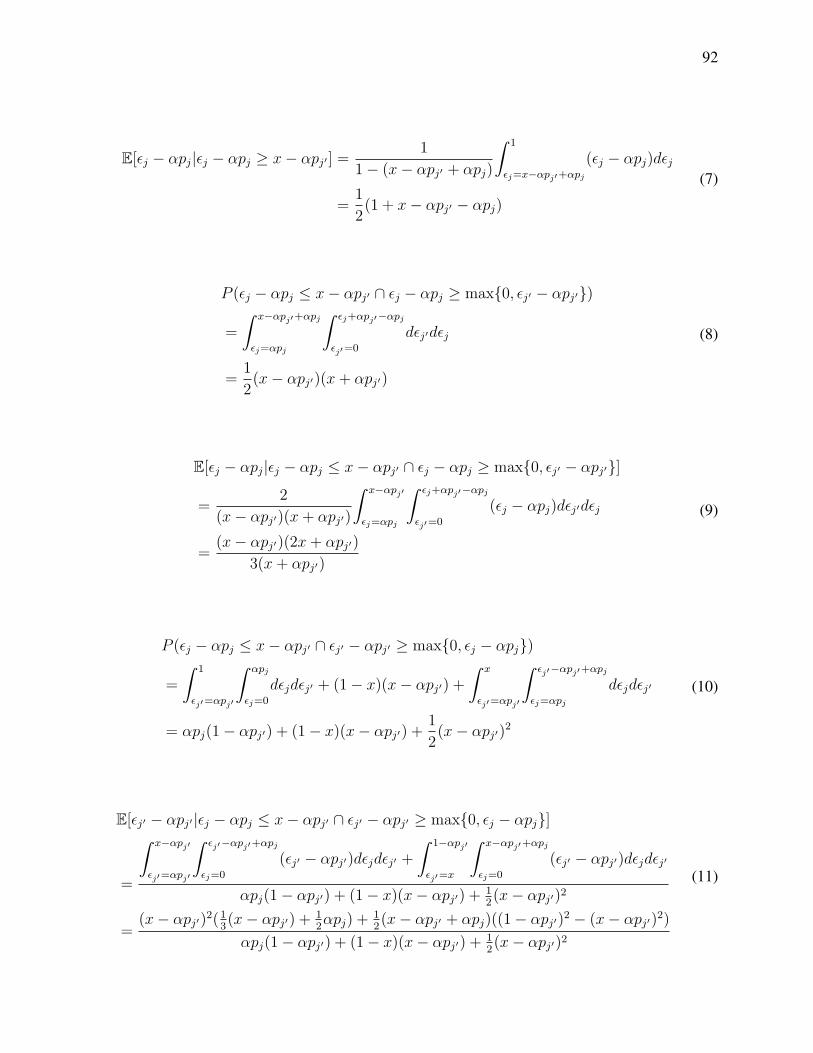
92
E[εj − αpj|εj − αpj ≥ x− αpj′ ] =1
1− (x− αpj′ + αpj)
∫ 1
εj=x−αpj′+αpj(εj − αpj)dεj
=1
2(1 + x− αpj′ − αpj)
(7)
P (εj − αpj ≤ x− αpj′ ∩ εj − αpj ≥ max{0, εj′ − αpj′})
=
∫ x−αpj′+αpj
εj=αpj
∫ εj+αpj′−αpj
εj′=0
dεj′dεj
=1
2(x− αpj′)(x+ αpj′)
(8)
E[εj − αpj|εj − αpj ≤ x− αpj′ ∩ εj − αpj ≥ max{0, εj′ − αpj′}]
=2
(x− αpj′)(x+ αpj′)
∫ x−αpj′
εj=αpj
∫ εj+αpj′−αpj
εj′=0
(εj − αpj)dεj′dεj
=(x− αpj′)(2x+ αpj′)
3(x+ αpj′)
(9)
P (εj − αpj ≤ x− αpj′ ∩ εj′ − αpj′ ≥ max{0, εj − αpj})
=
∫ 1
εj′=αpj′
∫ αpj
εj=0
dεjdεj′ + (1− x)(x− αpj′) +∫ x
εj′=αpj′
∫ εj′−αpj′+αpj
εj=αpj
dεjdεj′
= αpj(1− αpj′) + (1− x)(x− αpj′) +1
2(x− αpj′)2
(10)
E[εj′ − αpj′ |εj − αpj ≤ x− αpj′ ∩ εj′ − αpj′ ≥ max{0, εj − αpj}]
=
∫ x−αpj′
εj′=αpj′
∫ εj′−αpj′+αpj
εj=0
(εj′ − αpj′)dεjdεj′ +∫ 1−αpj′
εj′=x
∫ x−αpj′+αpj
εj=0
(εj′ − αpj′)dεjdεj′
αpj(1− αpj′) + (1− x)(x− αpj′) + 12(x− αpj′)2
=(x− αpj′)2(13(x− αpj′) +
12αpj) +
12(x− αpj′ + αpj)((1− αpj′)2 − (x− αpj′)2)
αpj(1− αpj′) + (1− x)(x− αpj′) + 12(x− αpj′)2
(11)

93
s(1− P (εj − αpj ≥ x− αpj′)) = s(x− αpj′ + αpj) (12)
After algebraic manipulations of Equations (6)-(12), we have the following simplified
expression for E[U j]:
E[U j] =1
2− αpj + xαpj − xαpj′ − α2pjpj′ +
1
2x2 +
1
2α2p2j +
1
2α2p2j′
− 1
2x2αpj +
1
2x2αpj′ −
1
3x3 − 1
6α3p3j′ +
1
2α3p2j′pj
(13)
With the expression for E[UH ] in (4) and E[UL] in (13), we next define
U(x, αpL, αpH) , E[UL]− E[UH ] =1
3− x+ x2 − 1
2αpL + xαpL − xαpH −
1
3x3
− 1
2x2αpL +
1
2x2αpH −
1
6(αpL)
3 +1
2αpH +
1
6(αpH)
3
(14)
and we want to show that this is non-negative.
∂U
∂x(x, αpL, αpH) = (αpH − αpL)(x− 1)− (x− 1)2 ≤ 0, (15)
and therefore,
U(x, αpL, αpH) ≥ U(αpH , αpL, αpH)
since the conditions on the search cost s correspond to x ≤ αpH . Define
l(αpL, αpH) , U(αpH , αpL, αpH)
=1
3− 1
2αpH −
1
2αpL + αpLαpH −
1
2(αpL)(αpH)
2 − 1
6(αpL)
3 +1
3(αpH)
3.(16)
We have

94
∂l
∂αpL(αpL, αpH) = −
1
2(αpH − 1)2 − 1
3(αpL)
2 ≤ 0, (17)
which implies that l(αpL, αpH) is decreasing in αpL. Since αpL ≤ αpH ,
E[UL]− E[UH ] ≥ l(αpL, αpH) ≥ l(αpH , αpH) = −1
3(x− 1)3 ≥ 0, (18)
which concludes the proof of this case.
Case (b): 12(αpH − αpL)2 ≤ s ≤ 1
2(1− αpH)2
In this case, the search cost is small enough such that after viewing the first product j, the
customer will choose to incur the search cost to search product j′ 6= j with positive probability
< 1. Here, we have E[UL] and E[UH ] as defined in Equation (13) from case (a). Next, we define
U(x, αpL, αpH) , E[UL]− E[UH ] = αpH − αpL − 2xαpH + 2xαpL + x2αpH − x2αpL
− 1
6(αpH)
3 +1
6(αpL)
3 +1
2(αpH)
2(αpL)−1
2(αpL)
2(αpH)(19)
and we want to show that this is non-negative.
∂U
∂x(x, αpL, αpH) = 2(x− 1)(αpH − αpL) ≤ 0, (20)
and therefore,
U(x, αpL, αpH) ≥ U(1 + αpL − αpH , αpL, αpH)
since the conditions on the search cost s correspond to x ≤ 1 + αpL − αpH . Define

95
l(αpL, αpH) , U(1 + αpL − αpH , αpL, αpH)
=5
6(αpH)
3 − 5
6(αpL)
3 − 5
2(αpL)(αpH)
2 +5
2(αpL)
2(αpH).(21)
We have
∂l
∂αpL(αpL, αpH) = −
5
2(αpL − αpH)2 ≤ 0, (22)
which implies that l(αpL, αpH) is decreasing in αpL. Since αpL ≤ αpH ,
E[UL]− E[UH ] ≥ l(αpL, αpH) ≥ l(αpH , αpH) = 0, (23)
which concludes the proof of this case.
Case (c): 12(1− αpH)2 ≤ s ≤ 1
2(αpH − αpL)2
In this case, if the customer views product L first, the search cost is prohibitively large such
that she would never incur a search cost to search product H . We have
E[UL] = E[max{0, εL − αpL}] = 12(1− αpL)2. However, if the customer views product H first,
the search cost is small enough such that she will always choose to search product L, regardless
of her realization of εH , and her utility is as defined in Equation (4). We define
U(x, αpL, αpH) , E[UL]− E[UH ] =1
3− 1
2αpL +
1
2αpH −
1
2(αpH)
2
+1
6(αpH)
3 + αpLαpH −1
2(αpL)(αpH)
2 − x+ 1
2x2
(24)
and we want to show that this is non-negative.
∂U
∂x(x, αpL, αpH) = x− 1 ≤ 0, (25)

96
and therefore,
U(x, αpL, αpH) ≥ U(αpH , αpL, αpH)
since the conditions on the search cost s correspond to x ≤ αpH . Define
l(αpL, αpH) , U(αpH , αpL, αpH)
=1
3− 1
2αpL −
1
2αpH +
1
6(αpH)
3 + αpLαpH −1
2(αpL)(αpH)
2.(26)
We have
∂l
∂αpL(αpL, αpH) = −
1
2(1− αpH)2 ≤ 0, (27)
which implies that l(αpL, αpH) is decreasing in αpL. Since αpL ≤ 2αpH − 1,
E[UL]− E[UH ] ≥ l(αpL, αpH)
≥ l(2αpH − 1, αpH) =5
6− 5
2αpH +
5
2(αpH)
2 − 5
6(αpH)
3 ≥ 0,(28)
which concludes the proof of this case.
Case (d): max{12(1− αpH)2, 12(αpH − αpL)
2} ≤ s ≤ 12(1− αpL)2
In this case, if the customer views product L first, the search cost is prohibitively large such
that she would never incur a search cost to search product H . We have
E[UL] = E[max{0, εL − αpL}] = 12(1− αpL)2. However, if the customer views product H first,
the search cost is small enough such that she will choose to search product L with positive
probability < 1, and her expected utility is as defined in Equation (13) for j = H, j′ = L. We
want to show

97
E[UH ] =1
2− αpH + xαpH − xαpL − α2pHpL +
1
2x2 +
1
2α2p2H +
1
2α2p2L
− 1
2x2αpH +
1
2x2αpL −
1
3x3 − 1
6α3p3L +
1
2α3p2LpH
≤ 1
2(1− αpL)2 = E[UL]
(29)
Rearranging terms, this inequality can be rewritten as
f(x, αpL, αpH) , −1
3x3 +
1
2x2 − xαpL + xαpH +
1
2x2αpL −
1
2x2αpH −
1
6(αpL)
3
+ αpL − αpH +1
2(αpH)
2 +1
2(αpL)
2αpH − (αpL)(αpH) ≤ 0
(30)
We have
∂f
∂x= (1− x)(x− αpL) + αpH(1− x) ≥ 0, (31)
where the inequality holds because our conditions on s equate to the following conditions on x:
αpL ≤ x ≤ min{αpH , 1 + αpL − αpH}. This means that for any αpL and αpH , f(x, αpL, αpH)
is increasing in x. Thus, in order to show f(x, αpL, αpH) ≤ 0, it suffices to show
f(min{αpH , 1 + αpL − αpH}, αpL, αpH) ≤ 0.
Consider each of the following two subcases:
Case (d.1): αpH ≤ 1 + αpL − αpH
In this subcase, we want to show f(αpH , αpL, αpH) ≤ 0. Let
g(αpL, αpH) , f(αpH , αpL, αpH) = −5
6(αpH)
3 + 2(αpH)2 − 2(αpL)(αpH)
+1
2(αpL)(αpH)
2 +1
2(αpL)
2(αpH)−1
6(αpL)
3 + αpL − αpH(32)
We will first argue that g(αpL, αpH) is increasing in αpL and will subsequently use this to

98
complete the proof.
∂g
∂αpL(αpL, αpH) = −2αpH +
1
2(αpH)
2 + αpLαpH −1
2(αpL)
2 + 1 (33)
This expression is decreasing in αpH because
∂2g
∂αpL∂αpH(αpL, αpH) = −2 + αpH + αpL ≤ 0. (34)
Thus ∂g∂αpL
(αpL, αpH) achieves its minimum value when αpH is at its maximum value,
which for the conditions in this subcase is when αpH = 12(1 + αpL). This gives us
∂g
∂αpL(αpL, αpH) ≥
∂g
∂αpL(αpL,
1
2(1 + αpL)) =
1
8(1− αpL)2 > 0. (35)
Therefore g(αpL, αpH) is increasing in αpL. Noting αpL ≤ αpH , we have
g(αpL, αpH) ≤ g(αpH , αpH) = 0 (36)
which concludes the proof of this subcase.
Case (d.2): αpH ≥ 1 + αpL − αpH
In this case, we want to show f(1 + αpL − αpH , αpL, αpH) ≤ 0. Let
h(αpL, αpH) , f(1 + αpL − αpH , αpL, αpH) =1
6(1 + αpL − αpH)3 −
1
6(αpL)
3
− (αpL)2 + (αpL)(αpH)−
1
2(αpH)
2 +1
2(αpL)
2(αpH)
(37)
We will first argue that h(αpL, αpH) is increasing in αpL and will subsequently use this to
complete the proof.

99
∂h
∂αpL(αpL, αpH) =
1
2(1 + αpL − αpH)2 −
1
2(αpL)
2 − 2αpL + αpH + (αpL)(αpH) (38)
This expression is increasing in αpH because
∂2h
∂αpL∂αpH(αpL, αpH) = αpH ≥ 0. (39)
Thus ∂h∂αpL
(αpL, αpH) achieves its minimum value when αpH is at its minimum value,
which for the conditions in this subcase is when αpH = 12(1 + αpL). This gives us
∂h
∂αpL(αpL, αpH) ≥
∂h
∂αpL(αpL,
1
2(1 + αpL)) =
1
4(1− αpL)2 +
1
2> 0. (40)
Therefore h(αpL, αpH) is increasing in αpL. Noting αpL ≤ 2αpH − 1, we have
h(αpL, αpH) ≤ h(2αpH − 1, αpH) =5
6(αpH)
3 − 5
2(αpH)
2 +5
2αpH −
5
6≤ 0 (41)
which concludes the proof of this subcase.
Case (e): s ≥ 12(1− αpL)2
In this case, the search cost is large enough such that the customer would only consider the
initial product viewed for purchase and would never incur a search cost to search the second
product. We simply have for j ∈ {L,H}
E[U j] = E[max{0, εj − αpj}] =1
2(1− αpj)2.
Since pL ≤ pH , we have E[UL] ≥ E[UH ].

100
Proof of Theorem 1
We prove each statement separately below.
Theorem 1(i):
Consider a customer who may face two possible scenarios: one scenario where she views
product L first and the other scenario where she views product H first. We will argue that she will
either purchase a product in both scenarios (could be different products) or not purchase a product
in either scenario. This implies that conversion (purchase probability) is the same for both
scenarios and, together with Lemma 1, implies that conversion would be the same regardless of if
a customer was in the control or treatment group.
Note that since s ≤ 12(1− αpH)2, a customer will always choose to search the second
product before choosing not to buy either product, i.e. the customer will purchase a product if
max{εj − αpj, εj′ − αpj′} ≥ 0. There are 4 possible search and purchase outcomes to consider,
given the customer viewed product j first.
1. The customer purchases product j without searching product j′. This implies
max{εj − αpj, εj′ − αpj′} ≥ εj − αpj ≥ 0, and thus the customer also would have
purchased a product if she were to have viewed product j′ first.
2. The customer purchases product j after searching product j′. This implies
max{εj − αpj, εj′ − αpj′} = εj − αpj ≥ 0, and thus the customer also would have
purchased a product if she were to have viewed product j′ first.
3. The customer purchases product j′. This implies
max{εj − αpj, εj′ − αpj′} = εj′ − αpj′ ≥ 0, and thus the customer also would have
purchased a product if she were to have viewed product j′ first.
4. The customer does not purchase either product. This implies
max{εj − αpj, εj′ − αpj′} < 0, and thus the customer also would not have purchased either
product if she were to have viewed product j′ first.
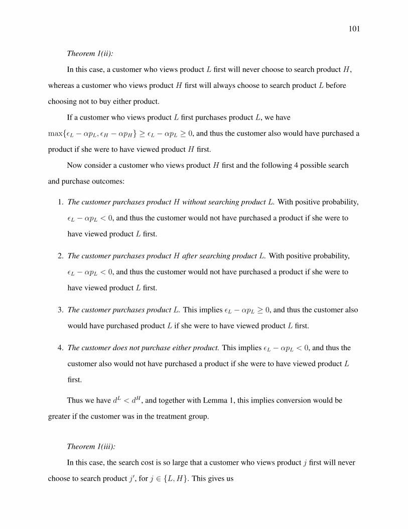
101
Theorem 1(ii):
In this case, a customer who views product L first will never choose to search product H ,
whereas a customer who views product H first will always choose to search product L before
choosing not to buy either product.
If a customer who views product L first purchases product L, we have
max{εL − αpL, εH − αpH} ≥ εL − αpL ≥ 0, and thus the customer also would have purchased a
product if she were to have viewed product H first.
Now consider a customer who views product H first and the following 4 possible search
and purchase outcomes:
1. The customer purchases product H without searching product L. With positive probability,
εL − αpL < 0, and thus the customer would not have purchased a product if she were to
have viewed product L first.
2. The customer purchases product H after searching product L. With positive probability,
εL − αpL < 0, and thus the customer would not have purchased a product if she were to
have viewed product L first.
3. The customer purchases product L. This implies εL − αpL ≥ 0, and thus the customer also
would have purchased product L if she were to have viewed product L first.
4. The customer does not purchase either product. This implies εL − αpL < 0, and thus the
customer also would not have purchased a product if she were to have viewed product L
first.
Thus we have dL < dH , and together with Lemma 1, this implies conversion would be
greater if the customer was in the treatment group.
Theorem 1(iii):
In this case, the search cost is so large that a customer who views product j first will never
choose to search product j′, for j ∈ {L,H}. This gives us

102
dL = 1− αpL > 1− αpH = dH , (42)
and together with Lemma 1, this implies conversion would be greater if the customer was in the
control group.
Proof of Theorem 2
We prove Theorem 2 separately for different ranges of the search cost, s.
Case (a): s ≤ 12(1− αpH)2
We first prove that dHH ≥ dLH , i.e. the demand for product H will be greater when the
customer views product H first. It suffices to show that a customer who views product L first and
purchases product H would also have purchased product H if she viewed product H first. Note
that in order for a customer who views product L first to purchase product H , she must have
searched product H and thus we know max{εH − αpH , εL − αpL} = εH − αpH . If instead the
customer were to view product H first, she would either purchase product H without searching
product L, or would search product L and then purchase product H since
max{εH − αpH , εL − αpL} = εH − αpH .
We next compare revenues:
dLLpL + dLHpH = (dL − dLH)pL + dLHpH = (dH − dLH)pL + dLHpH
≤ (dH − dHH)pL + dHHpH = dHL pL + dHHpH ,
(43)
where the second equality holds because dH = dL from Theorem 1, and the inequality holds
because pL < pH and dHH ≥ dLH . Together with Lemma 1, this concludes our proof for this case.
Case (b): 12(1− αpH)2 < s ≤ 1
2(1− αpL)2

103
In this case, we have
dLLpL + dLHpH = dLpL < dHpL < dHL pL + dHHpH , (44)
where the first inequality follows from Theorem 1 and the second inequality follows from
pH > pL. Together with Lemma 1, this concludes our proof for this case.
Case (c): s > 12(1− αpL)2
In this case, note that dj = djj = 1− αpj and thus the expected revenue of a customer who
views product j first is (1− αpj)pj . This is a parabola maximized at pj = 12α
, and thus the
expected revenue is largest for a customer who views product L first if and only if
|(1− αpL)pL − 12α| ≤ |(1− αpH)pH − 1
2α|; together with Lemma 1, this concludes our proof of
this case.
Proof of Theorem 3
Similar to the proof of Theorem 1, we prove each statement separately below. Note that a
customer has a positive probability of searching the second product j only if her expected benefit
of searching j exceeds her search cost s, i.e. if
s ≤∫ ∞εj=−∞
max{0, εj − αpj}fj(εj)dεj =∫ ∞εj=αpj
(εj − αpj)fj(εj)dεj.
Theorem 3(i):
Since s ≤ min{∫ ∞
εL=αpL
(εL − αpL)fL(εL)dεL,∫ ∞εH=αpH
(εH − αpH)fH(εH)dεH}
, a
customer will always choose to search the second product before choosing not to buy either
product, i.e. the customer will purchase a product if max{εj − αpj, εj′ − αpj′} ≥ 0. The proof for
this statement is identical to that of Theorem 1(i).
Theorem 3(ii):

104
In this case, a customer who views product L first will never choose to search product H ,
whereas a customer who views product H first will always choose to search product L before
choosing not to buy either product. The proof for this statement is identical to that of Theorem
1(ii).
Theorem 3(iii):
The proof for this case is identical to the proof for case (ii) after swapping L and H .
Theorem 3(iv):
In this case, the search cost is so large that a customer who views product j first will never
choose to search product j′. This gives us
dj =
∫ ∞εj=αpj
fj(εj)dεj, (45)
and thus the product that maximizes this quantity will lead to greater demand if viewed first.
Proof of Theorem 4
We prove Theorem 4 separately for different ranges of the search cost, s.
Case (a): s ≤ min{∫ ∞
εL=αpL
(εL − αpL)fL(εL)dεL,∫ ∞εH=αpH
(εH − αpH)fH(εH)dεH}
The proof of this case is identical to the proof of case (a) in Theorem 2, where dH = dL
from Theorem 3.
Case (b):∫ ∞εH=αpH
(εH − αpH)fH(εH)dεH < s ≤∫ ∞εL=αpL
(εL − αpL)fL(εL)dεL
In this case, we have
dLLpL + dLHpH = dLpL < dHpL < dHL pL + dHHpH , (46)

105
where the first inequality follows from Theorem 3 and the second inequality follows from
pH > pL.