the impact of incentives on human behavior: can we …

NBER WORKING PAPER SERIES

THE IMPACT OF INCENTIVES ON HUMAN BEHAVIOR:CAN WE MAKE IT DISAPPEAR? THE CASE OF THE DEATH PENALTY

Naci H. MocanR. Kaj Gittings

Working Paper 12631http://www.nber.org/papers/w12631

NATIONAL BUREAU OF ECONOMIC RESEARCH1050 Massachusetts Avenue

Cambridge, MA 02138October 2006

We thank Paul Mahler and Weijia Wu for excellent research assistance and Ted Joyce, Michael Grossman,Steve Medema, Laura Argys, and Erdal Tekin for helpful comments and suggestions. The views expressedherein are those of the author(s) and do not necessarily reflect the views of the National Bureau ofEconomic Research.

© 2006 by Naci H. Mocan and R. Kaj Gittings. All rights reserved. Short sections of text, not to exceedtwo paragraphs, may be quoted without explicit permission provided that full credit, including © notice,is given to the source.

The Impact of Incentives on Human Behavior: Can We Make It Disappear? The Case of theDeath PenaltyNaci H. Mocan and R. Kaj GittingsNBER Working Paper No. 12631October 2006JEL No. K0,K14,K4,K42

ABSTRACT

Although decades of empirical research has demonstrated that criminal behavior responds to incentives,non-economists frequently express the belief that human beings are not rational enough to make calculateddecisions about the costs and benefits of engaging in crime and therefore, a priori drawing the conclusionthat criminal activity cannot be altered by incentives. However, scientific research should not be drivenby personal beliefs. Whether or not economic conditions matter or deterrence measures such police,arrests, prison deaths, executions, and commutations provide signals to people is an empirical question,which should be guided by a solid theoretical framework. In this paper we extend the analysis of Mocanand Gittings (2003). We alter the original model in a number of directions to make the relationshipbetween homicide rates and death penalty related outcomes (executions, commutations and removals)disappear. We deliberately deviate from the theoretically consistent measurement of the risk variablesoriginally employed by Mocan and Gittings (2003) in a variety of ways. We also investigate the sensitivityof the results to changes in the estimation sample (removing high executing states for example) andweighting. The basic results are insensitive to these and a variety of other specification tests performedin the paper. The results are often strong enough to even hold up under theoretically meaninglessmeasurements of the risk variables. In summary, the original findings of Mocan and Gittings (2003)are robust, providing evidence that people indeed react to incentives induced by capital punishment.Research findings about the deterrent effect of the death penalty evoke strong feelings, which couldbe due to political, ideological, religious, or other personal beliefs. Yet, such findings do not meanthat capital punishment is good or bad, nor does it provide any judgment about whether capital punishmentshould be implemented or abolished. It is simply a scientific finding which demonstrates that peoplereact to incentives. Therefore, there is no need to be afraid of this result.

Naci H. MocanDepartment of EconomicsUniversity of ColoradoCampus Box 181; P.O. Box 173364Denver, CO 80217-3364and [email protected]

R. Kaj GittingsCornell UniversityDepartment of Economics391 Pine Tree RoadIthaca, NY [email protected]

1

The Impact of Incentives on Human Behavior: Can We Make It Disappear? The Case of the Death Penalty

“Get your facts first, and then you can distort ‘em as much as you please.” Mark Twain as quoted by Rudyard Kipling in From Sea to Sea (1914, p.180)

I. Introduction

Economists are interested in the investigation of human behavior and how

individuals respond to prices and incentives. Economic theory, which demonstrates an

inverse relationship between the price of a commodity and its consumption, similarly

suggests that an increase in the price or cost of a behavior leads to a reduction in the

intensity of that behavior. Therefore, as economic analysis of consumer behavior is

applicable to any commodity ranging from apples to cars, it is also applicable to any type

of human behavior, ranging from drunk driving to sexual activity to marital dissolution.

Based on economic theory, an immense amount of empirical research has investigated

the extent to which individuals alter their behavior in response to increases in the relevant

“prices” that may impact that behavior.

Rationality and Reaction to Incentives

One common argument made by non-economists against the economic approach

to human behavior is that people are not rational enough to behave according to the

predictions of economic theory when it comes to behaviors such as smoking,

consumption of alcohol and illicit drugs, sexual activity and crime. However, an

enormous empirical literature in economics has demonstrated that even these behaviors

are responsive to prices and incentives. For example, consumption of cigarettes declines

2

when cigarette prices rise (e.g., Becker, Murphy and Grossman, 1994; Yurekli and Zhang

2000; Gruber, Sen, and Stabile, 2003), alcohol consumption is curtailed when alcohol

prices are increased (e.g., Farrell, Manning and Finch 2003, Manning, Blumberg and

Moulton 1995), drug use responds to variations in drug prices, (e.g., van Ours 1995;

Saffer and Chaloupka 1999; Grossman 2005), pregnancies and childbearing are

influenced by state and federal policies that alter the costs (e.g. Mellor 1998; Lundberg

and Plotnick 1995), and the timing of births within a year is responsive to the tax benefit

of having a child (Dickert-Conlin and Chandra, 1999). Such results hold true even in

sub-populations such as adolescents, who are thought to be present-oriented and less

rational (e.g., Pacula et al. 2001; Gruber and Zinman 2001; Grossman and Chaloupka

1998; Grossman et al. 1994; Lundberg and Plotnick 1990), and among individuals with

mental health problems (Saffer and Dave 2005). In a different vein, research in

experimental economics has demonstrated that individuals respond to changes in prices

as predicted by economic theory, and even children behave rationally when modifying

their behavior in response to variations in prices (Harbaugh et al. 2001).

The same results are obtained from analyses of the response of criminal activity to

the relevant costs and benefits. The pioneering work of Becker (1968) indicates that

criminal activity should decline as the “price” of such activity increases. In his Nobel

Lecture on December 9, 1992, Becker stated that

“In the 1950s and 1960s intellectual discussions of crime were dominated by the opinion that criminal behavior was caused by mental illness and social oppression, and that criminals were helpless “victims.”… I explored instead the theoretical and empirical implications of the assumption that criminal behavior is rational (see the early pioneering work by Bentham [1931] and Beccaria [1986]), but again “rationality” did not necessarily imply narrow materialism. It recognized that many people are constrained by moral and ethical

3

considerations, and did not commit crimes even when they were profitable and there was no danger of detection. However, police and jails would be unnecessary if such attitudes always prevailed. Rationality implied that some individuals become criminals because of the financial rewards from crime compared to legal work, taking into account of the likelihood of apprehension and conviction, and the severity of punishment.”

Empirical analyses testing the economic model of crime have demonstrated that

illicit behavior indeed responds to incentives and sanctions. For example, Jacob and

Levitt (2003) show that incentives for high test scores motivated teachers and

administrators to cheat on standardized tests in Chicago public schools. Corman and

Mocan (2000, 2005) and DiTella and Schargrodsky (2004) demonstrate that increased

arrests and more police officers reduce crime. Levitt (1998a) shows that juvenile crime

goes down when punishment gets stiffer. Grogger (1998) and Mocan and Rees (2005)

find that the extent of criminal involvement among high school students is influenced by

both economic conditions and deterrence. Similarly, it has been shown that prison

crowding, which generates early release of prisoners, has a significant impact on crime

rates (Levitt 1996).

One specific sub-analysis in this domain has received significant attention.

Specifically, the extent to which homicide rates respond to deterrence was first

investigated theoretically and empirically by Ehrlich (1973, 1975, 1977), who found a

deterrent effect of capital punishment. Some analysts questioned the robustness of the

results (Hoenack and Weiler 1980; Passell and Taylor, 1977), and Ehrlich and others

responded to these criticisms (Ehrlich and Mark 1977, Ehrlich and Brower 1987, Ehrlich

and Liu 1999).

4

Robustness of Research Findings

Because no one single research paper can provide the final answer to a particular

scientific question, it is always important for second-generation researchers to investigate

the robustness of the findings in the original work. Recent examples of such activity

include the debate on the impact of guns on crime, and the relationship between abortion

and crime. Lott and Mustard (1997) reported evidence on the negative impact of

concealed weapons laws on crime. Subsequently, other researchers investigated the

robustness of the original results (Plassmann and Tideman 2001; Moody 2001; Ayres and

Donohue III 2003; Plassmann and Whitley 2003). Similarly, following the paper by

Donohue III and Levitt (2001) which documents a negative relationship between abortion

and crime, a debate has surged whether the findings are reflective of a causal impact

(Joyce 2004a; Donohue III and Levitt 2004b; Joyce 2004; Foote and Goetz 2005;

Donohue III and Levitt 2006).1

Along the same lines, in a recent article Donohue III and Wolfers (2006)

(D-III&W hereafter) focus on a number of papers that reported a deterrent effect of death

penalty on homicide, and claim that the findings of these papers are not robust. One

section of the D-III&W piece concentrates on Mocan and Gittings (2003), but it does not

provide an accurate representation of the findings of Mocan and Gittings (2003), or the

robustness of the results. The purpose of this paper is to provide a detailed sensitivity

analysis regarding the impact of leaving death row (executions, commutations and other

removals from death row) on state homicide rates. Specifically, we make various

1 Examples of other debates include the impact of the minimum wage laws and the schooling reform.

5

attempts to eliminate the deterrent effect of capital punishment and investigate if and

under what conditions one succeeds in eliminating the impact of leaving death row on the

homicide rate.

As we demonstrate in detail below, the signaling effect of leaving death row and

its impact on homicide is robust. Although the impact of executions disappears when one

estimates peculiar specifications as was done by D-III&W (which are inconsistent with

theory), the impact of commutations remains significant even in those models. And, as

described in the paper in detail, and summarized in Table 15, in many cases the results do

not disappear under other specifications that have no theoretical foundation.

II. The Empirical Model

Following Mocan and Gittings (2003), the investigation of the impact of

deterrence on homicide is carried out by estimating models of the following form:

(1) MURDERit = Dit-1 β + Xit Ω +μi +ηt +Ρit+ε it,

where MURDERit is the homicide rate in state i and year t. The vector X contains state

characteristics that may be correlated with criminal activity, including the unemployment

rate, real per capita income, the proportion of the state population in the following age

groups: 20-34, 35-44, 45-54 and 55 and over, the proportion of the state population in

urban areas, the proportion which is black, the infant mortality rate, the party affiliation

of the governor, and the legal drinking age in the state. Theoretical and empirical

justification for the inclusion of these variables can be found in Levitt

(1998a), and Lott and Mustard (1997). The variable μi represents unobserved state-

specific characteristics that impact the murder rate, and ηt represents year effects. To

6

control for the impact of the 1995 Oklahoma City bombing, a dummy variable is

included which takes the value of one in Oklahoma in 1995 and zero elsewhere. The

models also include state-specific time-trends represented by Ρit.

Measurement of risks (increase and decrease in the cost of murder)

The vector D represents deterrence variables, and includes the probability of

apprehension, the probability of sentencing given apprehension, as well as various

probabilities pertaining to leaving death row, conditional on sentencing.

It is important to note that execution is not the only outcome for prisoners on

death row. During the period of 1977-97 (the time period analyzed), among the inmates

who completed their duration on death row, 17 percent were executed. The other 83

percent left death row for other reasons (e.g. commutation of the sentence, sentence or

conviction being overturned, sentence being found unconstitutional). This information

allows for an investigation as to how the murder rate reacts to an increase in the price of

crime (executions) and a decrease in the price of crime (commutation, and all removals

other than executions and deaths).

It is important to define these probabilities appropriately at the outset. Once their

proper measurements are understood, they can be manipulated to make the deterrence

result disappear. The first one of these probabilities is the probability of apprehension

given committing murder. The second one is the probability of conviction given

apprehension, and the third one is the probability of execution (or commutation) given

conviction.

7

The probability of apprehension is a measure of the risk of getting caught, given

that a murder is committed. Because the unit of analysis is state-year, this probability is

measured as the proportion of murders cleared by an arrest in a particular state and year;

i.e. ARRATEt =(ARt/MURt), where ARt is the number of homicide arrests in a state in

year t (state subscript is dropped for ease of exposition), and MURt stands for the number

of homicides in year t.

The second risk variable is the probability of receiving a death sentence, given

that a murder arrest took place. This probability is measured as the proportion of people

convicted for murder from the pool of individuals who were arrested for murder.2 After

a person is arrested for murder, he/she does not automatically end up on death row.

Instead, a trial takes place. Furthermore, each person who goes to trial is not

automatically found guilty. Therefore, one can calculate the probability of being found

guilty and being sentenced to death following a trial, conditional on being arrested for

murder. The average duration between the date of a murder arrest and the date on which

an inmate is sentenced to death is more than one year.3 Thus, the risk of receiving the

death sentence is defined as the number of death sentences handed out in a year divided

by the number of murder arrests two years prior. That is, SENTRATEt= (SENTt/ARt-2),

where SENTt represents the number of death sentences handed out in year t.

If a person receives the death sentence after the trial, he/she is not executed

instantly. Ignoring this point (as was done by D-III&W) will be helpful in attempts to

make some of the results disappear. But the reality is, researchers recognized that the

2 That is, if 100 individuals are arrested for murder and 10 of them are subsequently convicted, the risk of conviction is 10%. 3 For example, a person who is arrested in October 1990, is likely to receive a death sentence after February 1992.

8

average duration on death row is about six years (Bedau 1997, Dezhbakhsh, Rubin and

Shepherd 2003, Mocan and Gittings 2003, Argys and Mocan 2004). About 83 percent of

the inmates are removed from death row for reasons other than execution. One such

reason is commutation, where the inmate is granted clemency and the sentence is

changed to a prison term, typically life. Because commutation implies a reduced risk of

death, and therefore a reduced cost of committing murder, an increase in the probability

of commutations should theoretically increase the homicide rate. The same argument is

true for all removals from death row (other than executions and other deaths while on

death row).

Therefore, following Mocan and Gittings (2003), three death penalty-related

deterrence variables are created. The first one is the risk of execution conditional on

being sentenced to death, the second one is the risk of being commuted conditional on

being sentenced to death, and the third one is the risk of being removed from death row

for reasons other than execution or other death conditional on being sentenced to death.

This third measure includes commutations, but is more comprehensive as it also includes

removals due to overturned sentence or conviction, or sentence being found

unconstitutional. According to economic theory, an increase in the first variable (the risk

of execution) should decrease the homicide rate as it makes murder more costly. On the

other hand, an increase in the second and third variables is expected to increase the

murder rate because an increase in the commutation or removal rate is associated with a

reduction in the cost of homicide.

Donohue III and Wolfers (2006) employ the data and methods of Mocan and

Gittings (2003), but they do not carefully consider the timing of events. They create

9

these variables as the ratio of executions (or removals) in a given year to the number of

death sentences in that same year, i.e. as (EXECt/SENTt), or (REMOVEt / SENTt).

Although useful in making the deterrence results disappear, these variables have no

meaning. This is because the numerator and denominator of the ratio have no connection

to each other. As discussed above, individuals who are sentenced to death in a given year

are not at risk of execution in that same year. However, by employing the ratio of

executions in year t to the death sentences in year t, D-III&W assume that execution of

each inmate takes place in the same year he/she was sentenced to death. As mentioned

earlier, the reality is that, after being sentenced to death, on average, death row inmates

face the event of execution or commutation about six years later; and the average

duration on death row for those who are removed from death row for reasons other than

death or execution is about five years (see Figure 10, which displays the progression of

the average duration on death row over time).

Although calculating these probabilities as was done by D-III&W is not sensible,

it would be reasonable to ask if the results were sensitive to variations in their proper

measurement. Specifically, we will consider variations in the probability of execution,

the probability of commutation, and the probability of removal from death row in three

different dimensions, and will investigate if these variations make the results disappear.

First, we will change the denominator of the risk variables to investigate if the results

disappear when we calculate the risks of execution, commutation and removals as

(EXECt/SENTt-5), (COMMt/SENTt-5), (REMOVEt/SENTt-5), assuming a five-year wait

on death row, and (EXECt/SENTt-4), (COMMt/SENTt-4), (REMOVEt/SENTt-4), assuming

a four-year wait. Put differently, we will investigate the sensitivity of the results to the

10

change in denominator of the risk variable, which is the average duration on death row.

By doing so, we move the lag lengths of the risk variables towards the direction favored

by D-III&W. Second, we will analyze whether alterations in the measurement of

execution risk, commutation risk and removal risk make the result disappear if the

numerators of these ratios are changed.

As described in detail in Mocan and Gittings (2003) an advantage of these data is

the availability of the date of each execution and removal, which enables one to create

execution, commutation and removal measures that are consistent with theory. If

executions, commutations or removals from death row send signals to potential criminals,

then the timing of the signal is important. For example, an execution which took place in

January of 1980 can have an impact on the homicide rate for the full year of 1980.

However, if the execution took place in December 1980, it will have a trivial impact on

the 1980 homicide rate. Rather, the impact of this December execution on murder will be

felt in 1981. Therefore, executions, commutations and removals are prorated based on

the month in which they occurred. As above, an execution that took place in January

1980 is expected to impact the state homicide rate for the entire twelve months in 1980.

Therefore we count this execution as a full execution in 1980. In contrast, if an execution

took place in November 1980, it is assumed that its deterrent impact on homicide is felt

during the subsequent 12-month period. Thus, this November execution counts as 2/12

of an execution for 1980 and 10/12 of an execution for 1981. The same algorithms are

applied for commutations and removals. We call these the first measure of executions,

commutations and removals. (This is the measure employed by Mocan and Gittings 2003,

and also Donohue III and Wolfers 2006).

11

As another measure, we created the following algorithm: If an execution took

place within the first three quarters of a year, we attributed that execution to the same

year. If the execution took place in the last quarter of a year (October-December) we

attributed that execution to the following year under the assumption that the relative

impact on murders would be felt in the following year. The same was done for removals

and commutations. We name these the second measures of executions, commutations

and removals (EXEC2, COMM2 and REMOVE2).

III. Let’s Make it Disappear

We estimate various versions of Equation (1). As was done in Mocan and

Gittings (2003), each specification controls for the following variables: The murder

arrest rate, the sentencing rate, the unemployment rate, real per capita income, the

proportion of the state population in the following age groups: 20-34, 35-44, 45-54 and

55 and over, the proportion of the state population in urban areas, the proportion which is

black, the infant mortality rate, governor’s party affiliation, and the legal drinking age in

the state. We control for state fixed-effects, a common time trend, state-specific time

trends, a dummy variable to control for the impact of the 1995 Oklahoma City bombing,

the number of prisoners per violent crime as well as the prison death rate: a measure of

prison conditions. These last two variables are included as additional measures of

deterrence, following Levitt (1998a), and Katz, Levitt and Shustorovich (2003).

Following Corman and Mocan (2000), Levitt (1998a), Katz Levitt and

Shistorovich (2003), and Mocan and Gittings (2003), the deterrence variables are lagged

12

by one year to minimize the concerns of simultaneity. For example, if the risk variable is

(EXECt/SENTt-5), its lagged value is employed in the regressions

[i.e. (EXECt/SENTt-5)-1 = (EXECt-1/SENTt-6)]. The models are estimated with weighted-

least squares, where the weights are state’s share in the U.S. population. Robust standard

errors, which are clustered at the state level, are reported in parentheses under the

coefficients. In the interest of space, only the coefficients and standard errors pertaining

to executions, commutations and removals are reported.

Table 1A displays the results where the first measures of execution, commutation

and removal are employed. These are the same measures used by Mocan and Gittings

(2003) and D-III&W. The only difference between D-III&W’s specification, the

specification used by Mocan and Gittings (2003), and the one reported in Table 1A is the

denominator of the execution, commutation and removal rates. Specifically, the top

panel of Table 1A measures the relevant risks as (EXECt/SENTt-5), (COMMt/SENTt-5),

(REMOVEt/SENTt-5). That is, it calculates the rates of execution, commutation and

removal per death sentences imposed 5 years earlier (assuming that the average duration

on death row is 5 years). The models presented in the middle panel of Table 1A are

identical, except, the average duration on death row is assumed to be 4 years. Thus, the

variables are calculated as (EXECt/SENTt-4), (COMMt/SENTt-4), and

(REMOVEt/SENTt-4).4

A number of aspects of the results in Table 1A are noteworthy. First, the point

estimates are very robust between specifications reported in the top two panels. Second,

4 Mocan and Gittings (2003) employed risk variables that take the average duration on death row as six years (denominator SENT lagged six years) in models for executions and commutations. Because the time between sentencing and REMOVE from death row is about 5 years, they employed SENT lagged five years in the denominator when the model included removals. Dohonue III and Wolfers (2006), on the other hand, use zero lags of SENT in the denominator.

13

the execution rate has a negative and statistically significant impact on the murder rate.

Third, the commutation and removal rates have positive impacts on the homicide rate.

Fourth, these results are consistent with the specifications reported in Mocan and Gittings

(2003), despite different lag lengths of the denominator (i.e. despite the fact that duration

on death row is assumed to be shorter than it really is).

The bottom panel of Table 1A displays the results of the model estimated by

D-III&W using the same data. In this specification, the execution, commutation and

removal rates are calculated by dividing executions, commutations and removals in a

year to the number of death sentences in that same year. Thus, they assume that the

duration on death row is less than one year. Similarly, in their specification, D-III&W

calculate the sentencing rate as the ratio of death sentences in a year to murder arrests in

that same year, assuming that the time length from arrest-to-trial-to-sentencing is less

than one year. This bizarre specification allows the execution result disappear, but even

this specification cannot eliminate the impact of commutations on the homicide rate.

Note that the equation on page 816 of D-III&W includes a variable called

(Pardonst-1 /DeathSentencest-7). D-III&W write that Mocan and Gittings (2003) estimate

that particular regression, although Mocan and Gittings (2003) do not employ pardons in

their paper. Similarly, Table 6 of D-III&W contains specifications in which a variable

named “Pardons” is included, and a discussion is provided about pardons.5 Mocan and

Gittings (2003) employed commutations in their regressions, not pardons.

Commutations and pardons are two unrelated events. A pardon invalidates the guilt and

5 For example, Donohue III and Wolfers state on page 818 that “… the two related measures of the porosity of the death sentence now yield sharply different results, with the pardon rate (emphasis added) robustly and positively associated with homicide…”

14

the punishment of the inmate. A commutation reduces the severity of punishment; it is

clemency, in which the sentence is reduced, typically to life in prison.

Table 1B reports results obtained from models where the executions,

commutations and removals are measured differently. Here we employ the second set of

variables as described in Section II above. In other words, the only difference between

results reported in Table1A and Table1B is the measurement of the numerator of the

execution, commutation, and removal rates. Once again, the impact of the execution

rates does not disappear, unless one estimates the peculiar specification promoted by D-

III&W; and similar to Table 1A, even in this case, the impact of the commutation rate on

the homicide rate is positive and statistically significant.

All Executions are in Texas

Donohue III and Wolfers (2006) write that California and Texas are very

interesting states which contain substantial and useful information for establishing the

deterrent effect of the death penalty, but suggest that the results may be sensitive to

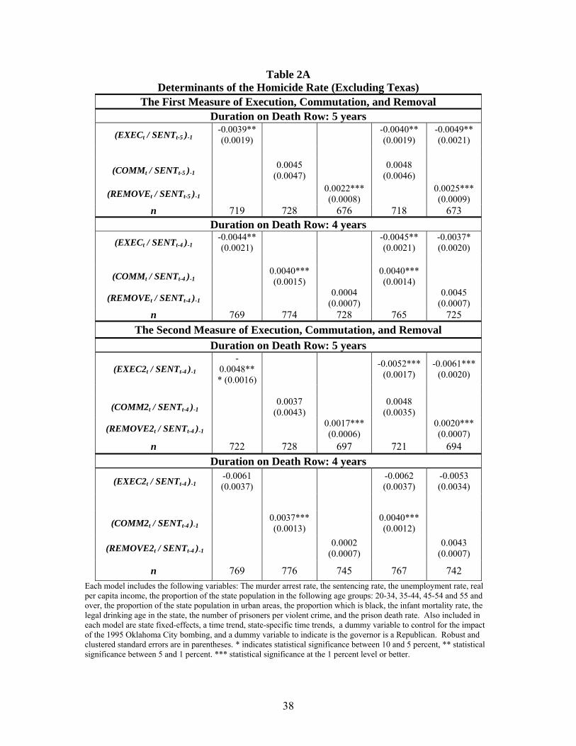
exclusion of Texas and California from the analysis (D-III&W p.826). Table 2A displays

the results obtained from models estimated with two different death row durations, and

two different ways to measure risk. Therefore, Table 2A is comparable to the top two

panels in Tables 1A and 1B with one difference: Texas is omitted from the models.

Table 2B is similar to Table 2A, except these regressions omit California. As the tables

demonstrate, these attempts to make the results disappear are not successful either. As

another attempt at disappearance, we excluded both Texas and California, and ran the

15

regressions without both states. The results, reported in Table 2C, show that the impact

of executions and commutations or removals are still significant when Texas and

California are both omitted from the analysis.

The Importance of the Denominator Once Again

Why is it the case that omitting Texas does not make the results disappear despite

the fact that Texas executes a disproportionately large number of death row inmates?

One obvious fallacy is to focus on executions when the correct measure is not the number

of executions, but the risk of the execution. Put differently, the number of executions

needs to be adjusted by the appropriate denominator, which is the number of death

sentences relevant for the cohort of death row inmates. Despite the fact that a particular

state has a large number of executions, the execution risk may not be high if the cohort of

inmates that was sentences to death 4-5 years earlier is also large.

In Table 3 we summarize the number of executions, commutation, and removals

from death row for other reasons between 1977 and 1997 for selected states; and also

present the average execution risk in each state during that period. The first measure is

the number of executions in year t divided by number of death sentences 4 years earlier.

The second measure deflates the number of executions by death sentences 5 years prior.

The third and fourth measures displayed in the table are the number of executions divided

by prison population (EXECt/PRISONt), and the number of executions deflated by the

number of inmates on death row in the same year (EXECt/ROWt), respectively. We will

discuss the relevance of these last two measures in detail below, but suffice it to say that

Texas is not the highest ranked state by any of these execution risks. It is ranked 4th or

16

5th, depending on the risk measure, behind Virginia, Arkansas, and Louisiana. Missouri

is generally ranked as the 5th state in execution risk. Therefore attempts to make the

results disappear would be more productive if one were to omit these states.

Tables 4A-4C present the results obtained from models when Virginia, Arkansas

or Louisiana are dropped, respectively. In each case, dropping these states does not

influence the results. That is, even when we remove the high-risk states from the

analysis, the results are still robust. This may not be all that surprising, as the coefficients

are estimated through the variations in the variables within a state.

This analysis shows that attempts to make the deterrence results disappear are

ineffective. Even if one estimates an unusual specification as was done by D-III&W

(replicated in the bottom panels of Table 1A and Table 1B) the estimated impact of

executions becomes statistically insignificant, but the positive impact of commutations on

the murder rate does not disappear.

IV. The Impact of Death Penalty Laws

Donohue III and Wolfers (2006) indicate in their paper that they use our data and

programs and analyze “the death penalty effects” separately for each state, making sure to

control for the same variables as in [the] main specification.” They claim that what they

find is the following: homicide rates were higher in Kansas and New Hampshire after

these states adopted the death penalty; lower in New York and New Jersey after their

adoption of the death penalty; and homicide rates declined in Massachusetts and Rhode

Island after these states abolished the death penalty (D-III&W, p. 809).

17

In making this claim, D-III&W do not report any regression results. We

estimated various models in an effort to substantiate their assertion. Because they

indicate that they estimated the impact of the death penalty laws separately for each of

the mentioned states controlling for the same variables as in the main models, we

estimated models separately for Massachusetts, Rhode Island, Kansas, New Hampshire,

New York and New Jersey. For each state a dummy variable is created that takes the

value of one if the death penalty is legal, and zero otherwise. Kansas legalized the death

penalty in 1994. New Hampshire legalized it in 1991. Legalization took place in 1982

and 1995 for New Jersey and New York, respectively. Massachusetts and Rhode Island

abolished the death penalty in 1984.6 Because the sample runs from 1977 to 1997,

running regressions for each state separately is complicated by a degrees-of-freedom

problem. Nevertheless, in an effort to verify the statement of D-III&W, we ran five

different models for each state while varying the number of control variables. The results

are reported in Tables 5A-5F. The number of control variables differs between the

specifications to investigate the sensitivity. The sentencing rate could only be included in

the regressions for New Jersey, because there is no variation in the number of death

sentences in the five other states. Similarly, the drinking age cannot be included in the

models. As the tables show, inclusion or exclusion of control variables has no substantial

impact on the estimated coefficients of legal death penalty indicator. In these

regressions, the coefficient of the death penalty indicator is not statistically different from

zero in Kansas, Massachusetts, Rhode Island, and New York. It is negative and

significant in New Hampshire and New Jersey. Thus, these results strikingly contradict 6 Massachusetts abolished the death penalty in October 1984. Thus, 1985 is the first year with no death penalty in Massachusetts in the data since abolishment took place. Similarly, 1985 is the first full year where the death penalty is illegal in Rhode Island.

18

the claim of D-III&W. For example, D-III&W claim that the adoption of the death

penalty increased the homicide rate in Kansas, whereas Table 5A demonstrates that the

impact was to reduce the homicide rate (by the sign of the coefficients), or at best, was

not statistically significant. Regardless, the results suggest that the impact was certainly

not to increase in homicide rate in Kansas. D-III&W make the same claim for New

Hampshire that there was an increase in the homicide rate after the adoption of capital

punishment. Table 5B, though, suggests just the opposite. The same is true for their

claims pertaining to other states, with the exception of New Jersey. D-III&W write that

the abolishment of the death penalty reduced the homicide rate in Massachusetts and

Rhode Island. Tables 5C and 5D, however, demonstrate that the impact, although not

significant, is in the opposite direction of their claim: the homicide rate was lower when

the death penalty was legal in those states, not higher, although it is not estimated with

precision. Only New Jersey is consistent with their claim (Table 5F), as the adoption of

the death penalty generated a decline in the homicide rate.

How could D-III&W’s claims be so different from those obtained from regression

results? It is possible that D-III&W based their statement on a different type of analysis.

Somewhere else in their paper, while discussing a different work, they mention that

dummy variables are created for each “experiment” of death penalty adoption or abolition

in a state, which takes the value of one for that state subsequent to the law change.7 Thus,

in that analysis, they examine the impact of each state-specific intervention by pooling all

the data. Following this logic, we created six state-specific dummy variables (one for

each state mentioned), which take the value of one for a particular state after the law

change in that state. Pooling all the data and estimating models with all control variables 7 Page 807, where D-III&W discuss Dezhbakhsh and Shepherd (2004).

19

and also adding these intervention variables produced coefficients for these

“experiments” that were consistent with the D-III&W statement, but their statistical

significance was not. Specifically, the p-values of coefficients of the “experiment”

variables in Massachusetts and Rhode Island were 0.23, and 0.40, respectively.

Thus, it appears that D-III&W’s statement is based on point estimates,

disregarding the statistical in-significance of these estimates. Ignoring this issue, we

should point out that many of these point estimates conflict with those reported in Tables

5A-5F. We suggest the following explanation. Their “experiment” variable is an

interaction between the state dummy and the legal dummy to indicate the legality of

death penalty in that state. However, it seems like D-III&W do not fully interact the state

dummy with the other right hand side variables. That is, they implicitly assume that the

effects of all the other right hand side variables (arrest rate, unemployment rate,

sentencing rate, percent black, etc.) are the same across states. This could be a major

concern for the meaningfulness of estimates obtained from pooled data if the restrictive

assumption that the secondary effects of the other control variables are zero turns out to

be incorrect. A fully-interacted model does not make this assumption, nor does running

the regressions separately for each state. However, because a common time component

across states is estimated in the pooled data, one can no longer obtain the usual one-to-

one mapping between the estimates of the fully interacted model and those from the state-

specific regressions.

In an attempt to find a middle ground, we estimated the fully interacted model and

included time dummies. Unfortunately, the model is so saturated that many of the

estimates are no longer identified due to collinearities. However, as one moves from the

20

D-III&W pooled model and includes more and more secondary effects the results change

significantly. For example, when we estimated the pooled regression where the state

dummies are interacted with only two explanatory variables (homicide arrest rate and

prisoners per violent crime), the coefficient for Kansas became insignificant, the

coefficients on New Hampshire and New York flipped signs and were significant, and the

coefficient on New Jersey became insignificant.

As an alternative analysis of the direction of the impact of each state’s death

penalty laws, we performed an interrupted time-series analysis. Figures 1A and 2A

present the time-series behavior of the homicide rates in Kansas and New Hampshire

since 1960. These states legalized the death penalty in 1994 and in 1991, respectively.

Although D-III&W assert that the homicide rate went up in these states after the

legalization, Figures 1A and 2A suggest that the opposite may be the case. D-III&W

write that the homicide rates went down in New York and New Jersey after legalization

(Figures 3A and 4A), but they claim the homicide rates also went down in Massachusetts

and Rhode Island (presented in Figures 5A and 6A) due to the abolishment of the death

penalty. Figure 5A shows that there was an increase in the homicide rate in

Massachusetts after the law change, followed by a drop in 1997. It is uncertain whether

this drop can be attributable to the change in law 12 years prior. In the case of Rhode

Island, the homicide rate is fluctuating around a quadratic trend, and the level of the

homicide rate seems to have increased, rather than decreased, after the abolition.

To investigate if the “experiment” in a state has altered the behavior of the

homicide rate in that state over time, we employed well-defined intervention analysis

methods. The time-series dynamics of the homicide rate of each state can be modeled

21

separately, and intervention variables can be added to investigate if the change in the

death penalty law in that state in a particular year has altered the time-series dynamics of

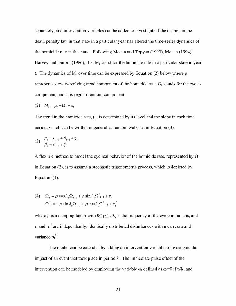
the homicide rate in that state. Following Mocan and Topyan (1993), Mocan (1994),

Harvey and Durbin (1986), Let Mt stand for the homicide rate in a particular state in year

t. The dynamics of Mt over time can be expressed by Equation (2) below where μt

represents slowly-evolving trend component of the homicide rate, Ωt stands for the cycle-

component, and εt is regular random component.

(2) ttttM εμ +Ω+=

The trend in the homicide rate, μt, is determined by its level and the slope in each time

period, which can be written in general as random walks as in Equation (3).

(3) ttt

tttt

ξββηβμμ

+=++=

−

−−

1

11

A flexible method to model the cyclical behavior of the homicide rate, represented by Ω

in Equation (2), is to assume a stochastic trigonometric process, which is depicted by

Equation (4).

(4) *

1*

1*

1*

1

cossin

sincos

ttctct

ttctct

τλρλρ

τλρλρ

+Ω+Ω−=Ω

+Ω+Ω=Ω

−−

−−

where ρ is a damping factor with 0≤ ρ≤1, λc is the frequency of the cycle in radians, and

τt and τt* are independently, identically distributed disturbances with mean zero and

variance σt2.

The model can be extended by adding an intervention variable to investigate the

impact of an event that took place in period k. The immediate pulse effect of the

intervention can be modeled by employing the variable ωt defined as ωt=0 if t≠k, and

22

ωt=1 if t=k. If the intervention shifts the level of the variable, then the intervention

variable ωt is defined as ωt=0 if t≠k, and ωt=1 if t≥ k, and ttttt ηδωβμμ +++= −− 11 .

We estimated the model, depicted by Equations (2)-(4) by including the

intervention variables. The models are first estimated from 1977 forward to be consistent

with the time period used in the earlier analyses. The estimated trend values along with

actual data are displayed in Figures 1B-6B. As can be seen, in the four states that

adopted the death penalty, the “experiment” had altered the dynamics of the homicide

rate by reducing its level. In the two states that abolished the death penalty on the other

hand, the level of the homicide rate has increased.8

As another set of analyses, we estimated the models starting in 1960, except for

New York, where the data are available starting in 1965. This allows us to investigate the

impact of the adoption of the death penalty in South Dakota (in 1979), New Mexico (in

1979) and in Oregon (in 1978). Furthermore, we can also jointly investigate the impact

of the 1972 Supreme Court moratorium. The results are presented graphically in Figures

1C-9C. In each case, the Furman decision is associated with an increase in the level of

the homicide rate. Consistent with the dynamics presented in Figures 1B-6B, adoption of

the death penalty generated declines in the homicide trends, and abolition in

Massachusetts and Rhode Island produced increases in the homicide rate, although long-

run trends in these series generated subsequent declines.

8 Although the death penalty was legal during period before 1984 in Massachusetts, the 1970s and 1980s witnessed a series of legislation and judicial rulings regarding the death penalty. Identifying these time intervals and considering interventions associated with them did not alter the picture depicted in Figure 5B. The same, to a lesser degree, is true for Rhode Island where the death penalty was re-enacted in 1977, but in 1979 the Rhode Island Supreme Court issued the opinion of the violation of the prohibitions of the 8th amendment of the U.S. constitution (Rhode Island Secretary of State web site). Adding this potential intervention did not alter the picture depicted in Figure 6B.

23

Evidence from Panel Data

In this section, we investigate whether the existence of the death penalty in a state

has a separate impact on the homicide rate in addition to the risks associated with being

on the death row. To that end, we estimated the same models as those presented in

Tables 1A-4C, but we added a dichotomous indicator if death penalty is legal in a given

state in a particular year. Furthermore, we interacted this dummy variable with the

execution rate, commutation rate and removal rate variables. These specifications are

estimated by Mocan and Gittings (2003) who deflated by risk measures by death

sentences given six years earlier (SENTt-6) in models with executions and commutations,

and by death sentences five years earlier in models with removals.

The results are displayed in Tables 6A and 6B, where the two alternative

measures of execution, commutation and removal risks are employed. In each case,

models are estimated with 4 and 5-lags of the death sentences in the denominator of the

risk variables as before. The results demonstrate that the existence of the death penalty in

a state has a negative and statistically significant impact on the homicide rate. In

addition, the execution rate has a negative impact on the homicide rate, and

commutations and removals have a positive impact, although not always statistically

significant. Once again, these results are consistent with those reported by Mocan and

Gittings (2003).

V. The Denominator of the Risk Variables Again

Although not realized by D-III&W, individuals who received a death sentence do

not exit the death row in the same year as they received the death sentence. To make the

24

point more visible, the average duration on death row is calculated each year for those

inmates who are removed that year, and plotted in Figure 10 by the reason of exit. As

can be inferred, individuals who were commuted, executed or otherwise removed from

death row had spent an average of about six years on death row. On the other had, those

who were executed or commuted in 1997 had completed about 11 years on death row.

Given this picture, one can use time-varying durations on death row to calculate the risks

of execution, commutation or removals. For example, the execution risk in year 1981

can be calculated as the number of executions in 1981 divided by the number of death

sentences in 1980 (because the duration on death row was one year in 1981). On the

other hand, the risk of execution in 1990 can be measured as the number of executions in

1990 divided by the number of death sentences in 1982 (because the average duration on

death row for those who were executed in 1990 was 8 years. See Figure 10). More

generally, the execution, commutation and removal rates are calculated as

(EXECt / SENTt-i), (COMMt / SENTt-j), and (REMOVEt / SENTt-k), where i, j and k are

average durations on death row for spells ending in year t for executions, commutations

and removals, respectively. Calculating the risks this way produced the results displayed

in Table 7. Once again, we are unsuccessful in eliminating the impact of the execution

risk on the homicide rate.9

Some researchers calculated the execution risk as the number of executions in a

year divided by the number of prisoners in that state in that year (e.g. Katz et al. 2003).

This calculation assumes that every prisoner in state correctional facilities is at risk of

being executed. This assumption has no validity as about 99.7 percent of the inmates in

9 Another extreme is to uniformly increase the lag length of the denominator. For example, when lag-length seven is imposed the same results are obtained, but not surprisingly, the statistically significance is lowered.

25

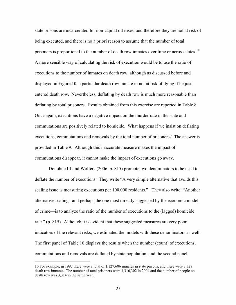
state prisons are incarcerated for non-capital offenses, and therefore they are not at risk of

being executed, and there is no a priori reason to assume that the number of total

prisoners is proportional to the number of death row inmates over time or across states.10

A more sensible way of calculating the risk of execution would be to use the ratio of

executions to the number of inmates on death row, although as discussed before and

displayed in Figure 10, a particular death row inmate in not at risk of dying if he just

entered death row. Nevertheless, deflating by death row is much more reasonable than

deflating by total prisoners. Results obtained from this exercise are reported in Table 8.

Once again, executions have a negative impact on the murder rate in the state and

commutations are positively related to homicide. What happens if we insist on deflating

executions, commutations and removals by the total number of prisoners? The answer is

provided in Table 9. Although this inaccurate measure makes the impact of

commutations disappear, it cannot make the impact of executions go away.

Donohue III and Wolfers (2006, p. 815) promote two denominators to be used to

deflate the number of executions. They write “A very simple alternative that avoids this

scaling issue is measuring executions per 100,000 residents.” They also write: “Another

alternative scaling –and perhaps the one most directly suggested by the economic model

of crime—is to analyze the ratio of the number of executions to the (lagged) homicide

rate.” (p. 815). Although it is evident that these suggested measures are very poor

indicators of the relevant risks, we estimated the models with these denominators as well.

The first panel of Table 10 displays the results when the number (count) of executions,

commutations and removals are deflated by state population, and the second panel

10 For example, in 1997 there were a total of 1,127,686 inmates in state prisons, and there were 3,328 death row inmates. The number of total prisoners were 1,316,302 in 2004 and the number of people on death row was 3,314 in the same year.

26

presents the results when they are deflated by lagged homicide rate as suggested by D-

III&W.

The dependent variable for the analysis is the homicide rate, which is measured as

homicides deflated by population. Thus, deflating executions by population, as suggested

by D-III&W, means that population enters into the denominator of both the dependent

and independent variables, inducing a positive bias in the estimated coefficient of the

execution rate. Despite this, the coefficient of the execution rate remains negative and

significant. Because the dependent variable of the analysis is the homicide rate, to use

the homicide rate as the deflator of executions is not meaningful.11 Nevertheless, we used

the lagged homicide rate as the deflator as promoted by D-II&W. As the send panel of

Table 10 demonstrates, even this trick did not make the results disappear.

VI. Further Attempts to Make the Results Disappear

The risk measures employed in this paper and also used in Mocan and Gittings

(2003) and D-III&W are calculated such that if there is an execution in a given state in a

given year, but it so happens that nobody was sentenced to death five years prior, then the

risk (EXECt/SENTt-5 ) cannot be calculated because the denominator is zero. On the

other hand, in cases where nobody was sentenced and nobody was executed, the

execution risk was taken as zero.

One can adopt an algorithm where observations are dropped from the data when

the corresponding death sentences are zero, regardless of the numerator of the risk

11 Donohue III and Wolfers seem to recognize this, and write that in their analysis they employ the lagged homicide rate as the deflator (D-III&W, ft. 63). However, if the homicide rate has any path-dependence, such as a simple AR(1) model, using the lagged-dependent variable in the denominator of the independent variable does not avoid a bias.

27

measure. This algorithm assumes that the risks cannot be calculated in cases when they

should be zero, such as the cases where there is no legal death penalty. Even so, and

despite the fact that this algorithm eliminates about half of the legitimate observations,

the impact of the death penalty on the homicide rate remains as shown in Tables 11A and

11B. Furthermore, although the irregular specification promoted by Donohue III and

Wolfers, (which assumes that the duration from arrest-to-sentencing and from

sentencing-to-execution, commutation or removal is less than one year) eliminates the

statistical significance of the execution variables, it cannot eliminate the significance of

commutations.

What happens to the results if we go to the extreme and use the number of

executions, commutations and removals as measures of risk, without deflating by

anything? Here, the scale of executions, commutations and removals are considered as

appropriate signals to individuals, rather than the rates at which they occur (as defined by

the correct denominator). Though we do not agree that this is the correct specification,

Table 12 shows that even this modification does not eliminate the impact of prices on

human behavior. Although the coefficients of commutations and removals are

statistically insignificant, the coefficient of execution remains significant even in this

model.

D-III&W argue that the deterrent impact of the death penalty which exists in

states with large populations such as New York and New Jersey exert disproportionate

influence in a population-weighted regression and overwhelms the no-deterrence result

that would have been obtained in regressions with no weighting. (Donohue III and

Wolfers 2006, footnote 50). To investigate if the results are driven by this hypothesis, we

28

estimated the models presented in Tables 1A and 1B without population weights. The

results are presented in Tables 13A and 13B. In models where the duration of death row

is taken as 5 years (the top panel), the results are actually stronger with the coefficients of

the commutation rate being significant. In the second panel of Tables 13A and 13B the

execution rate is insignificant, but the removal rate becomes significant when it was

insignificant in the weighted regression displayed in Tables 1A and 1B. Finally, the

results of the peculiar regression run by D-III&W remain unchanged whether the

regressions are weighted or not. Specifically, the bottom panels of Tables 13A and 13B

show that, even in their model an increase in commutations generates an increase in the

homicide rate as predicted by theory, and the coefficient of the removal rate becomes

significant in one specification.

In Table 14 we present the results obtained from the models that exclude New

York and New Jersey, and estimate the models without weighting. As can be seen, the

impact of leaving the death row on the homicide rate cannot be eliminated by dropping

New York and New Jersey from the analysis and running the regressions with no

weighting. The same conclusion is obtained, when we ran the models displayed in

Tables 2-6 with no weights. Thus, the results are not an artifact of weighting.

VII. Ph.D. Economists versus Criminals

In his Nobel lecture, Gary Becker described his inspiration for modeling

economic behavior of crime as follows.

“I began to think about crime in the 1960s after driving to Columbia University for an oral examination of a student in economic theory. I was late and had to decide quickly whether to put the car in a parking lot or risk getting a ticket for parking illegally on the street. I

29

calculated the likelihood of getting a ticket, the size of the penalty, and the cost of putting the car in a lot. I decided it paid to take the risk and park on the street. (I did not get a ticket.)

As I walked the few blocks to the examination room, it occurred to me that the city authorities had probably gone through a similar analysis. The frequency of their inspection of parked vehicles and the size of the penalty imposed on violators should depend on their estimates of the type of calculations potential violators like me would make.” (Becker 1992, p.42).

One standard objection to economic analysis of crime is that whether potential

criminals are as astute as Ph.D. economists to evaluate these probabilities accurately.

This objection is invalid so long as the researcher believes that empirical research should

be conceptually consistent with the underlying theory. If one assumes a priori that

individuals are incapable of calculating the risks as they are defined by theory, then there

is no room to conduct proper empirical research. For example, if one rejects the

theoretically-proper measure of the execution risk as executions within a cohort of death

row inmates in a given year divided by death sentenced handed out to that cohort in some

earlier year (because one believes that potential criminals do not observe either the

executions or the death sentences), then one ought to claim that they cannot observe and

evaluate other variables either, including the arrest rates, the size of the police force or

police spending. Thus, there would be no need to conduct research investigating

whether people react to deterrence, under the belief that people could not evaluate

variations in deterrence risks to begin with.

Furthermore, attempts to justify the use of inappropriate variables based on the

claim that individuals cannot observe, measure or determine the values of decision

parameters will produce peculiar analyses that cannot be defended theoretically. For

example, if the theory indicates that the real wages should matter in a particular context,

30

it would be silly to suggest the use of nominal wages in a regression (instead of real

wages) on the grounds that people cannot observe and predict accurately the level of the

consumer price index. If the theory indicates that the accident risk in a state is best

measured by the number of accidents per vehicle miles traveled, it would be incorrect to

promote deflating accidents by other measures such as the square miles of the state or the

number of car dealerships, on the grounds that vehicle miles traveled is difficult to

observe.

It should be noted, however, that in our context, the results are robust even to the

use of measures that are inconsistent with theory. A summary of the findings is provided

in Table 15, which displays the results obtained from estimating various versions of

Equation (1) along with the description of the measurement of the execution,

commutation and removal rates in each specification. The table displays results that are

obtained from specifications where the key variables (execution, commutation and

removal risks) are measured as dictated by theory. The table also presents results from

the models where they are measured incorrectly. Examples are the specifications

promoted by D-III&W (reported in rows 5 and 6 of Table 15), and the specifications

where the executions, commutations and removals are deflated by lagged murder rate, by

population, or where the raw count of executions, commutations and removals are used.

As the table demonstrates, the results are remarkably stable even across models that

substantially deviate from theory.

31

VIII. Conclusion and Discussion

Do people respond to incentives? An economist’s answer to this question is a

resounding “yes,” not only because economic theory indicates that incentives matter, but

because an enormous empirical literature shows that they do. An especially confusing

dimension for non-economists is the behavior of individuals in such domains as the

consumption of addictive substances, sexual activity and criminal behavior. In the case

of criminal behavior, non-economists frequently express the belief that human beings are

not rational enough to make calculated decisions about the costs and benefits of engaging

in crime, and that criminal activity cannot be altered by incentives. Of course personal

beliefs should not determine the answers to scientific questions such as whether the earth

is round or whether criminal behavior is responsive to incentives. Rather, answers should

be provided by careful and objective scientific inquiry.

In the economic approach to crime, decades of empirical research has

demonstrated that potential criminals indeed respond to incentives. It has been

documented that improved labor market conditions reduce the extent of criminal activity

(recent examples include Grogger 1998, Freeman and Rodgers 2000, Gould et al. 2002),

and criminal activity reacts to deterrence (e.g. Ehrlich 1975, Levitt 1998b, Kessler and

Levitt 1998, Corman and Mocan 2000, Mustard 2003, Corman and Mocan 2005). For

example, Levitt (1998b) showed that deterrence is empirically more important than

incapacitation in explaining crime, and that increases in arrest rates deter criminal

activity. Kessler and Levitt (1999) show that Proposition 8 in California, which

introduced sentence enhancements for certain crimes, reduced eligible crimes by 4

percent in the year following its passage and 8 percent 3 years after the passage,

32

providing strong evidence that crime rates react to the severity of punishment. In an

analysis of the relationship between crime and punishment for juveniles, Levitt (1998a)

finds that changes in relative punishment between juveniles and adults explain 60 percent

of the differential growth rates in juvenile and adult crime, and that abrupt changes in

criminal involvement with the transition from juvenile to adult courts indicate that

individuals do respond to the expected punishment (as economic theory suggests).

Corman and Mocan (2005, 2000) show that criminal activity responds to variations in

arrests and the size of the police force.

As discussed in the introduction, the signal provided by leaving death row is no

different from any other change in expected punishment. That is, an execution is a signal

of an increase in expected punishment, and a commutation represents a decrease in

expected punishment. However, it is sometimes claimed that because executions are

infrequent events, they cannot possibly be a strong enough signals to alter the behavior of

people. Yet, the same analysts have no difficulty in believing that a prospective criminal

observes correctly and accurately the extent of the increase in the number of arrests, and

coupled with the information about the level of crime, he calculates the enhanced risk of

getting caught, and changes his behavior. Similarly, the suggestion that if the local

authority hires 20 new police officers, the associated increase in the risk of getting caught

by this move is properly evaluated by potential criminals does not raise objections. Even

prison deaths are believed to provide signals to people who are not in prison. Katz, Levitt

and Shustorovich (2003) find that the death rate in prisons constitutes deterrence, and an

increase in prison deaths has a negative impact on crime rates. It is very difficult to argue

that an increase in prison deaths would be a signal of deterrence, but an increase in the

33

executions would not. However, this is the argument put forth by some analysts (e.g.

Donohue III and Wolfers 2006).

Clearly, analysts’ personal beliefs regarding what should and should not

constitute a strong signal are irrelevant. Whether or not police, arrests, prison deaths,

executions, or commutations provide signals to people about the extent of expected

punishment is an empirical question. In this paper we extend the analysis of Mocan and

Gittings (2003). We alter the original model in a number of directions to make the

relationship between homicide rates and death penalty related outcomes (executions,

commutations and removals) disappear. We change the measurement of the risk

variables by altering the numerator and the denominator of the variables in a variety of

ways (see Table 15 for a summary), we also investigate how the results change when we

exclude various states from the analysis. The basic results are insensitive to these and a

variety of other specification tests performed in the paper. The impact of executions

indeed becomes statistically insignificant when one estimates the specification promoted

by Donohue III and Wolfers (2006). However, that particular specification has little

theoretical relevance as we have explained in detail, and, furthermore, even that

specification cannot make the impact of commutations disappear.

It is understandable that the death penalty may evoke strong feelings. These

feelings could be due to political, ideological, religious, or other personal beliefs. The

reactions towards the research that identifies a deterrent effect of the death penalty

suggest that it may be difficult to isolate such feelings from objective evaluation of a

research finding. One reason may be the fear that a scientific paper which identifies a

deterrent effect could be taken as an endorsement or justification of the death penalty.

34

This should not be the case for any scientific research. This point is highlighted by

Mocan and Gittings (2003) and Katz,Levitt and Shustorovich (2003). For example, Katz,

Levitt and Shustorovich (2003) find that the death rate among prisoners (a proxy for

prison conditions) deters crime. This finding obviously does not suggest that the society

should increase the death rate of the prisoners by worsening the prison conditions to

reduce the crime rate. Nevertheless, the authors feel the need to state the obvious, and

write that:

“We cannot stress enough that evidence of a deterrent effect of poor prison conditions is neither a necessary nor a sufficient condition for arguing that current prison conditions are either overly benign or unjustifiably inhumane. Efficiency arguments related to deterrence are only one small aspect of an issue that is inextricably associated with basic human rights, constitutionality, and equity considerations. Our research is descriptive, not proscriptive.” (p.322)

Similarly, Mocan and Gittings (Mocan and Gittings 2003, p. 474) write that the

fact that there exists a deterrent effect of capital punishment, should not imply a position

on death penalty. There are a number of significant issues surrounding the death penalty,

ranging from potential racial discrimination in the imposition of the death penalty

(Baldus et al., 1998) to discrimination regarding who is executed and who is commuted

once the death penalty is received (Argys and Mocan 2004).

Although it is important to preserve objectivity in evaluating scientific research,

because of the nature of death penalty, it seem like ideologues, activists, and some

scientists also feel compelled to enter the debate with opinions formed based on selective

readings and half-truths. This unfortunate phenomenon is described succinctly by

Sunstein and Vermeule (2006), where they write in their reply to D-III&W:

35

“We cannot help but add that as new entrants into the death penalty debate, we are struck by the intensity of people’s beliefs on the empirical issues, and the extent to which their empirical judgments seem to be driven by their moral commitments. Those who oppose the death penalty on moral grounds often seem entirely unwilling to consider apparent evidence of deterrence and are happy to dismiss such evidence whenever even modest questions are raised about it. Those who accept the death penalty on moral grounds often seem to accept the claim of deterrence whether or not good evidence has been provided on its behalf.”

In summary, the original findings of Mocan and Gittings (2003) are robust,

providing evidence that people react to incentives in the domain of capital punishment.

Yet, this result does not imply that capital punishment is good or bad, nor does it provide

any judgment about whether capital punishment should be implemented or abolished. It

is just a scientific finding which demonstrates that people react to incentives. Therefore,

there is no need to be afraid of this result.

36

Table 1A Determinants of the Homicide Rate

The First Measure of Execution, Commutation, and Removal

Duration on death row: 5 years

(EXECt / SENTt-5 )-1 -0.0056** (0.0027) -0.0058**

(0.0028) -0.0066** (0.0029)

(COMMt / SENTt-5 )-1 0.0065 (0.0047) 0.0070

(0.0046)

(REMOVEt / SENTt-5 )-1 0.0024*** (0.0008) 0.0027***

(0.0009)

n 734 743 691 733 688


(EXECt / SENTt-4 )-1 -0.0054** (0.0022) -0.0055**

(0.0022) -0.0047** (0.0021)

(COMMt / SENTt-4 )-1 0.0036* (0.0021) 0.0038**

(0.0019)

(REMOVEt / SENTt-4 )-1 0.0004 (0.0007) 0.0005

(0.0007)

n 785 790 744 781 741

Donohue III & Wolfers specification

Duration on Death Row: 0 Years; Time between Arrest and Death Sentence: 0 Years

(EXECt / SENTt )-1 0.0003

(0.0014) 0.0001 (0.0013)

0.0001 (0.0014)

(COMMt / SENTt )-1 0.0041***

(0.0013) 0.0041*** (0.0013)

(REMOVEt / SENTt )-1 0.0002

(0.0003) 0.0002 (0.0003)

n 986 984 921 977 918 Each model includes the following variables: The murder arrest rate, the sentencing rate, the unemployment rate, real per capita income, the proportion of the state population in the following age groups: 20-34, 35-44, 45-54 and 55 and over, the proportion of the state population in urban areas, the proportion which is black, the infant mortality rate, the legal drinking age in the state, the number of prisoners per violent crime, and the prison death rate. Also included in each model are state fixed-effects, a time trend, state-specific time trends, a dummy variable to control for the impact of the 1995 Oklahoma City bombing, and a dummy variable to indicate is the governor is a Republican. Robust and clustered standard errors are in parentheses. * indicates statistical significance between 10 and 5 percent, ** statistical significance between 5 and 1 percent. *** statistical significance at the 1 percent level or better.

37

Table 1B Determinants of the Homicide Rate

The Second Measure of Execution, Commutation, and Removal

Duration on Death Row: 5 years

(EXEC2t / SENTt-5 )-1 -0.0058***

(0.0020) -0.0062*** (0.0022)

-0.0073*** (0.0022)

(COMM2t / SENTt-5 )-1 0.0044 (0.0047) 0.0056

(0.0040)

(REMOVE2t / SENTt-5 )-1 0.0018*** (0.0007) 0.0021***

(0.0007)

n 737 743 712 736 709


(EXEC2t / SENTt-4 )-1 -0.0069* (0.0035) -0.0070**

(0.0035) -0.0063* (0.0033)

(COMM2t / SENTt-4 )-1 0.0034* (0.0019) 0.0036**

(0.0016)

(REMOVE2t / SENTt-4 )-1 0.0002 (0.0008) 0.0005

(0.0007)

n 785 792 761 783 758

Donohue III & Wolfers specification Duration on Death Row: Zero Years; Time Between Arrest and Death Sentence: 0 Years

(EXEC2t / SENTt )-1 -0.0002 (0.0020) -0.0001

(0.0019) -0.00004 (0.0019)

(COMM2t / SENTt )-1 0.0039*** (0.0010) 0.0039***

(0.0001)

(REMOVE2t / SENTt )-1 -0.0002

(0.0006) -0.0002 (0.0006)


38

Table 2A Determinants of the Homicide Rate (Excluding Texas)

The First Measure of Execution, Commutation, and Removal Duration on Death Row: 5 years

(EXECt / SENTt-5 )-1 -0.0039** (0.0019) -0.0040**

(0.0019) -0.0049** (0.0021)

(COMMt / SENTt-5 )-1 0.0045 (0.0047) 0.0048

(0.0046)

(REMOVEt / SENTt-5 )-1 0.0022*** (0.0008) 0.0025***

(0.0009) n 719 728 676 718 673


(EXECt / SENTt-4 )-1 -0.0044** (0.0021) -0.0045**

(0.0021) -0.0037* (0.0020)

(COMMt / SENTt-4 )-1 0.0040*** (0.0015) 0.0040***

(0.0014)

(REMOVEt / SENTt-4 )-1 0.0004 (0.0007) 0.0045

(0.0007) n 769 774 728 765 725

The Second Measure of Execution, Commutation, and Removal Duration on Death Row: 5 years

(EXEC2t / SENTt-4 )-1

-0.0048*** (0.0016)

-0.0052*** (0.0017)

-0.0061*** (0.0020)

(COMM2t / SENTt-4 )-1 0.0037 (0.0043) 0.0048

(0.0035)

(REMOVE2t / SENTt-4 )-1 0.0017*** (0.0006) 0.0020***

(0.0007) n 722 728 697 721 694


(EXEC2t / SENTt-4 )-1 -0.0061 (0.0037) -0.0062

(0.0037) -0.0053 (0.0034)

(COMM2t / SENTt-4 )-1 0.0037*** (0.0013) 0.0040***

(0.0012)

(REMOVE2t / SENTt-4 )-1 0.0002 (0.0007) 0.0043

(0.0007)


39

Table 2B Determinants of the Homicide Rate (Excluding California)


(EXECt / SENTt-5 )-1 -0.0048* (0.0027) -0.0049*

(0.0028) -0.0059* (0.003)

(COMMt / SENTt-5 )-1 0.0050 (0.0047) 0.0054

(0.0046)

(REMOVEt / SENTt-5 )-1 0.0024*** (0.0008) 0.0027***

(0.0009)

n 719 728 677 718 674


(EXECt / SENTt-4 )-1 -0.0052** (0.0020) -0.0052**

(0.0020) -0.0047** (0.0019)

(COMMt / SENTt-4 )-1 0.0034 (0.0022) 0.0036*

(0.0020)

(REMOVEt / SENTt-4 )-1 0.0006 (0.0007) 0.0008

(0.0007)

n 769 774 729 765 726


(EXEC2t / SENTt-5 )-1 -0.0049** (0.0020) -0.0052**

(0.0021) -0.0065***

(0.0021)

(COMM2t / SENTt-5 )-1 0.0031 (0.0047) 0.0041

(0.0040)

(REMOVE2t / SENTt-5 )-1 0.0018*** (0.0006) 0.0021***

(0.0007)

n 722 728 697 721 694

Duration on Death Row: 4 years (EXEC2t / SENTt-4 )-1

-0.0063* (0.0032) -0.0063*

(0.0032) -0.0059* (0.003)

(COMM2t / SENTt-4 )-1 0.0032 (0.0020) 0.0033*

(0.0018)

(REMOVE2t / SENTt-4 )-1 0.0003 (0.0008) 0.0006

(0.0008)


40

Table 2C Determinants of the Homicide Rate (Excluding Texas and California)

The First Measure of Executions, Commutations, and Removals Duration on Death Row: 5 years

(EXECt / SENTt-5 )-1 -0.0029 (0.0019) -0.0030**

(0.0020) -0.0041* (0.0023)

(COMMt / SENTt-5 )-1 0.0048 (0.0043) 0.0051

(0.0042)

(REMOVEt / SENTt-5 )-1 0.0024*** (0.0008) 0.0026***

(0.0009) n 704 713 662 703 659

Duration on Death Row: 4 years (EXECt / SENTt-4 )-1

-0.0041** (0.0019) -0.0042**

(0.0019) -0.0036* (0.0018)

(COMMt / SENTt-4 )-1 0.0042*** (0.0011) 0.0043**

(0.0019)

(REMOVEt / SENTt-4 )-1 0.0007 (0.0007) 0.0008

(0.0007) n 753 758 713 749 710

The Second Measure of Executions, Commutations, and Removals Duration on Death Row: 5 years

(EXEC2t / SENTt-4 )-1 -0.0039** (0.0016) -0.0042**

(0.0017) -0.0054***

(0.0019)

(COMM2t / SENTt-4 )-1 0.0037 (0.0040) 0.0046

(0.0034)

(REMOVE2t / SENTt-4 )-1 0.0018*** (0.0006) 0.0020***

(0.0007) n 707 713 682 706 679


(EXEC2t / SENTt-4 )-1 -0.0055 (0.0034) -0.0056*

(0.0033) -0.0051 (0.0031)

(COMM2t / SENTt-4 )-1 0.0039*** (0.0011) 0.0040***

(0.0010)

(REMOVE2t / SENTt-4 )-1 0.0004 (0.0008) 0.0006

(0.0007)


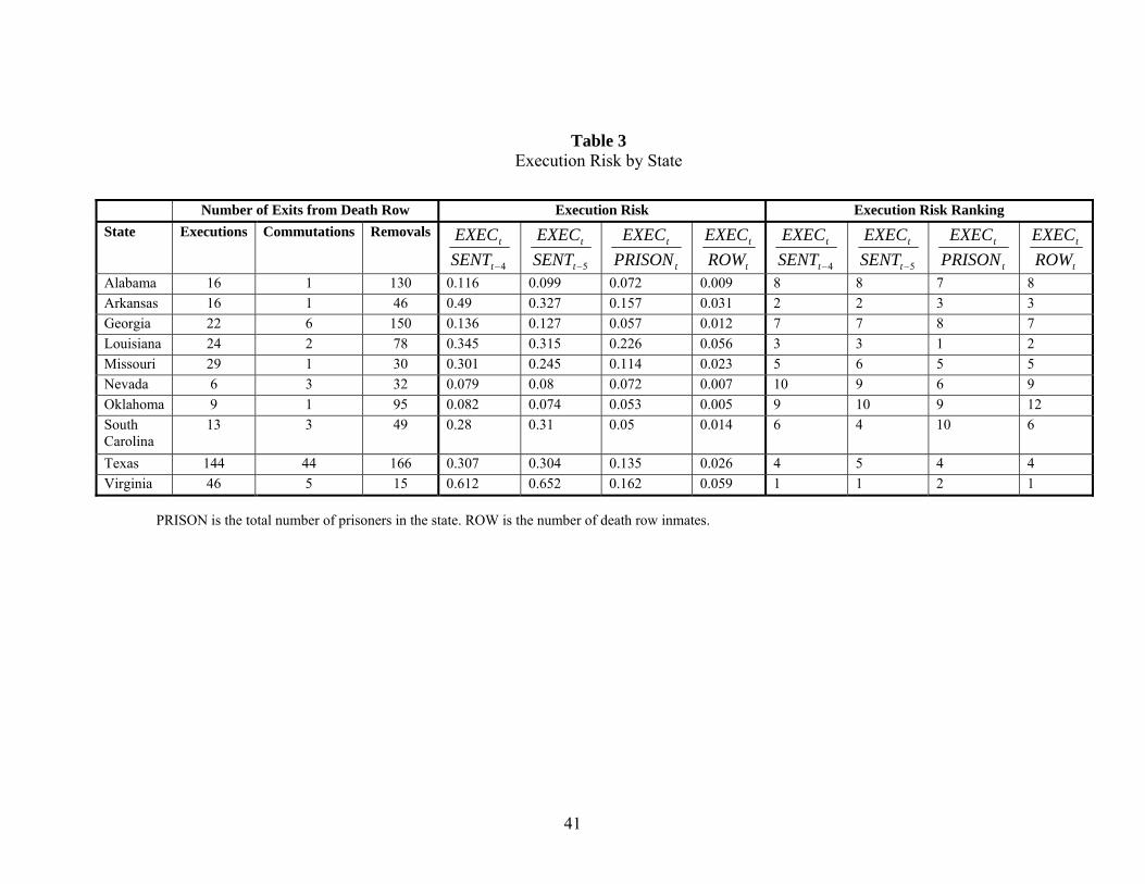
41

Table 3 Execution Risk by State

PRISON is the total number of prisoners in the state. ROW is the number of death row inmates.

Number of Exits from Death Row Execution Risk Execution Risk Ranking State Executions Commutations Removals

4−t

t

SENTEXEC

5−t

t

SENTEXEC

t

t

PRISONEXEC

t

t

ROWEXEC

4−t

t

SENTEXEC

5−t

t

SENTEXEC

t

t

PRISONEXEC

t

t

ROWEXEC

Alabama 16 1 130 0.116 0.099 0.072 0.009 8 8 7 8 Arkansas 16 1 46 0.49 0.327 0.157 0.031 2 2 3 3 Georgia 22 6 150 0.136 0.127 0.057 0.012 7 7 8 7 Louisiana 24 2 78 0.345 0.315 0.226 0.056 3 3 1 2 Missouri 29 1 30 0.301 0.245 0.114 0.023 5 6 5 5 Nevada 6 3 32 0.079 0.08 0.072 0.007 10 9 6 9 Oklahoma 9 1 95 0.082 0.074 0.053 0.005 9 10 9 12 South Carolina

13 3 49 0.28 0.31 0.05 0.014 6 4 10 6

Texas 144 44 166 0.307 0.304 0.135 0.026 4 5 4 4 Virginia 46 5 15 0.612 0.652 0.162 0.059 1 1 2 1

42

Table 4A Determinants of the Homicide Rate (Excluding Virginia)


(EXECt / SENTt-5 )-1 -0.0066* (0.0035) -0.0068*

(0.0037) -0.0084** (0.0036)

(COMMt / SENTt-5 )-1) 0.0087** (0.0038) 0.0091**

(0.0039)

(REMOVEt / SENTt-5 )-1 0.0025*** (0.0008) 0.0029***

(0.0010)

n 719 728 676 718 673


(EXECt / SENTt-4 )-1 -0.0052** (0.0025) -0.0052**

(0.0025) -0.0045* (0.0024)

(COMMt / SENTt-4 )-1 0.0044*** (0.0016) 0.0045***

(0.0015)

(REMOVEt / SENTt-4 )-1 0.0004 (0.0007) 0.0005

(0.0007)

n 769 774 728 765 725


(EXEC2t / SENTt-5 )-1 -0.0063** (0.0026) -0.0061**

(0.0026) -0.0083***

(0.0024)

(COMM2t / SENTt-5 )-1 0.0083*** (0.0030) 0.0083***

(0.0031)

(REMOVE2t / SENTt-5 )-1 0.0019*** (0.0007) 0.0023***

(0.0008)

n 722 728 697 721 694


-0.0066 (0.0040) -0.0067

(0.0040) -0.0060 (0.0037)

(COMM2t / SENTt-4 )-1 0.0043*** (0.0013) 0.0044***

(0.0012)

(REMOVE2t / SENTt-4 )-1 0.0003 (0.0008) 0.0005

(0.0007) n 769 776 745 767 742

Each model includes the following variables: The murder arrest rate, the sentencing rate, the unemployment rate, real per capita income, the proportion of the state population in the following age groups: 20-34, 35-44, 45-54 and 55 and over, the proportion of the state population in urban areas, the proportion which is black, the infant mortality rate, the legal drinking age in the state, the number of prisoners per violent crime, and the prison death rate. Also included in each model are state fixed-effects, a time trend, state-specific time trends, a dummy variable to control for the impact of the 1995 Oklahoma City bombing, and a dummy variable to indicate is the governor is a Republican. Robust and clustered standard errors are in parentheses. * indicates statistical significance between 10 and 5 percent, ** statistical significance between 5 and 1 percent. *** statistical significance at the 1 percent level or better.

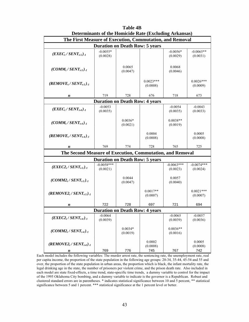
43

Table 4B Determinants of the Homicide Rate (Excluding Arkansas)


(EXECt / SENTt-5 )-1 -0.0055* (0.0028) -0.0056*

(0.0029) -0.0065** (0.0031)

(COMMt / SENTt-5 )-1 0.0065 (0.0047) 0.0068

(0.0046)

(REMOVEt / SENTt-5 )-1 0.0023*** (0.0008) 0.0026***

(0.0009)

n 719 728 676 718 673


(EXECt / SENTt-4 )-1 -0.0053 (0.0035) -0.0054

(0.0035) -0.0043 (0.0033)

(COMMt / SENTt-4 )-1 0.0036* (0.0021) 0.0038**

(0.0019)

(REMOVEt / SENTt-4 )-1 0.0004 (0.0008) 0.0005

(0.0008)

n 769 774 728 765 725


(EXEC2t / SENTt-5 )-1 -0.0058***

(0.0021) -0.0063*** (0.0023)

-0.0074*** (0.0024)

(COMM2t / SENTt-5 )-1 0.0044 (0.0047) 0.0057

(0.0040)

(REMOVE2t / SENTt-5 )-1 0.0017** (0.0007) 0.0021***

(0.0007)

n 722 728 697 721 694


-0.0064 (0.0039) -0.0065

(0.0039) -0.0057 (0.0036)

(COMM2t / SENTt-4 )-1 0.0034* (0.0019) 0.0036**

(0.0016)

(REMOVE2t / SENTt-4 )-1 0.0002 (0.0008) 0.0005

(0.0008) n 769 776 745 767 742


44

Table 4C Determinants of the Homicide Rate (Excluding Louisiana)


(EXECt / SENTt-5 )-1 -0.0059 (0.0035) -0.0063*

(0.0036) -0.0071* (0.0038)

(COMMt / SENTt-5 )-1 0.0080* (0.0041) 0.0086**

(0.0041)

(REMOVEt / SENTt-5 )-1 0.0022** (0.0009) 0.0024**

(0.0009)

n 720 728 678 719 675


(EXECt / SENTt-4 )-1 -0.0041* (0.0023) -0.0042*

(0.0023) -0.0041* (0.0024)

(COMMt / SENTt-4 )-1 0.0041*** (0.0015) 0.0042***

(0.0014)

(REMOVEt / SENTt-4 )-1 0.0006 (0.0007) 0.0008

(0.0007)

n 770 774 730 766 727


(EXEC2t / SENTt-5 )-1 -0.0060** (0.0026) -0.0067**

(0.0026) -0.0063** (0.0026)

(COMM2t / SENTt-5 )-1 0.0058 (0.0043) 0.0072**

(0.0034)

(REMOVE2t / SENTt-5 )-

1 0.0017**

(0.0008) 0.0018** (0.0008)

n 722 728 699 721 696


-0.0039 (0.0027) -0.0040

(0.0027) -0.0039 (0.0028)

(COMM2t / SENTt-4 )-1 0.0039*** (0.0014) 0.0040***

(0.0013)

(REMOVE2t / SENTt-4 )-

1 0.0005

(0.0007) 0.0006 (0.0007)


45

TABLE 5A The Impact of the Death Penalty on the Homicide Rate

Kansas (1) (2) (3) (4) (5)

-0.0214 -0.0044 -0.0007 -0.008* -0.0011 Death Penalty Legal (-1) (0.0220) (0.0183) (0.0061) (0.0040) (0.0033)

0.0296 0.0112 0.0293** 0.0275* Homicide Arrest Rate (-1) (0.0225) (0.0109) (0.0105) (0.0146)

-0.003 -0.0441 -0.08*** -0.0856** Prisoners per Violent Crime (-1) (0.0675) (0.0498) (0.0160) (0.0210)

-0.0116 -0.0091 0.0059* Prison Death Rate (-1) (0.0063) (0.0057) (0.0031)

0.0066 0.0041 0.0019 Percent Black (0.0041) (0.0042) (0.0015)

-0.0098* -0.0098** -0.015** Republican Governor (0.0031) (0.0023) (0.0045) Unemployment Rate -0.0019 (0.0021)

-0.0338 -0.0287* -0.0253** -0.0073 Per Capita Income (0.0134) (0.0126) (0.0065) (0.0061) Infant Mortality Rate 0.0005 (0.0043) Urbanization 0.0499 (0.0667) Percent Aged 20 - 34 -0.04 -0.0457** -0.0268** (0.0145) (0.0103) (0.0069) Percent Aged 35 - 44 -0.0608 -0.055** -0.0244** (0.0274) (0.0171) (0.0085) Percent Aged 45 - 54 -0.0245 -0.0365** -0.0177** (0.0195) (0.0100) (0.0067) Percent Aged 55+ 0.013* 0.0097** 0.0074**

(0.0039) (0.0016) (0.0027)

0.0076 0.0159** 0.0072** 0.0026** 0.0014*** Time Trend (0.0106) (0.0054) (0.0029) (0.0008) (0.0003)

Robust and clustered standard errors in parentheses. * statistical significance between 10 and 5 percent, ** statistical significance between 5 and 1 percent. *** statistical significance at the 1 percent level or better.

46

TABLE 5B The Impact of the Death Penalty on the Homicide Rate

New Hampshire (1) (2) (3) (4) (5)

-0.0226 -0.0253** -0.0125 -0.0206** -0.0213** Death Penalty Legal (-1) (0.0119) (0.0099) (0.0105) (0.0080) (0.0078)

-0.0051 0.0005 0.0013 0.0004 Homicide Arrest Rate (-1) (0.0038) (0.0027) (0.0023) (0.0019)

0.0412 0.0566 0.0182 0.0168 Prisoners per Violent Crime (-1) (0.0377) (0.0304) (0.0161) (0.0140)

0.0004 0.0006 0.0005 Prison Death Rate (-1) (0.0013) (0.0011) (0.0007)

-0.001 0.0013 0.0022 Percent Black (0.0053) (0.0025) (0.0042)

-0.01 -0.0046 -0.0011 Republican Governor (0.0063) (0.0042) (0.0049) Unemployment Rate 0.0013 (0.0033)

0.0069 0.0033 -0.0007 0.0001 Per Capita Income (0.0108) (0.0037) (0.0039) (0.0026) Infant Mortality Rate -0.0046 (0.0030) Urbanization -0.0796 (0.0423) Percent Aged 20 - 34 -0.0031 0.0091 0.0029 (0.0120) (0.0083) (0.0104) Percent Aged 35 - 44 0.0032 -0.017 -0.0102 (0.0166) (0.0103) (0.0112) Percent Aged 45 - 54 0.0053 -0.0006 -0.003 (0.0220) (0.0138) (0.0176) Percent Aged 55+ -0.0079 -0.0027 -0.0032

(0.0069) (0.0046) (0.0038)

-0.0183 0.0055 0.006 -0.0003 -0.0001 Time Trend (0.0142) (0.0047) (0.0050) (0.0017) (0.0008)


47

TABLE 5C

The Impact of the Death Penalty on the Homicide Rate Massachusetts

(1) (2) (3) (4) (5) -0.0055 -0.0059 -0.0082* -0.0075 -0.0066 Death Penalty Legal (-1) (0.0060) (0.0048) (0.0045) (0.0065) (0.0051)

0.0028 0.0017 -0.0022 -0.002 Homicide Arrest Rate (-1) (0.0103) (0.0061) (0.0062) (0.0047)

-0.0932 -0.1127 -0.1152 -0.1253 Prisoners per Violent Crime (-1) (0.1731) (0.1374) (0.1178) (0.0762)

0.0012 0.0008 -0.0001 Prison Death Rate (-1) (0.0044) (0.0021) (0.0012)

-0.0022 -0.0021 -0.0015 Percent Black (0.0046) (0.0019) (0.0017)

-0.0069 -0.0058 -0.0043 Republican Governor (0.0133) (0.0098) (0.0084)

Unemployment Rate 0.0004 (0.0026)

-0.0149 -0.0151 -0.0159** -0.0005 Per Capita Income (0.0203) (0.0088) (0.0071) (0.0034) Infant Mortality Rate 0.00003 (0.0073) Urbanization -0.0287 (0.1967) Percent Aged 20 - 34 0.0124 0.0127* 0.0152** (0.0145) (0.0063) (0.0059) Percent Aged 35 - 44 0.0384 0.0358 0.0299 (0.0522) (0.0205) (0.0190) Percent Aged 45 - 54 0.0309 0.0309 0.0324* (0.0371) (0.0177) (0.0167) Percent Aged 55+ -0.0051 -0.0041 -0.0045

(0.0144) (0.0025) (0.0027)

-0.0078 -0.0079 -0.0068 0.0003 0.0003 Time Trend (0.0098) (0.0061) (0.0057) (0.0006) (0.0006)


48

TABLE 5D The Impact of the Death Penalty on the Homicide Rate

Rhode Island (1) (2) (3) (4) (5)

-0.0087 -0.0051 -0.0043 -0.0034 -0.0063 Death Penalty Legal (-1) (0.0046) (0.0096) (0.0070) (0.0076) (0.0067)

0.0264 -0.0025 -0.0142 -0.0135 Homicide Arrest Rate (-1) (0.0155) (0.0222) (0.0131) (0.0105)

0.0851 0.0235 -0.0089 -0.0086 Prisoners per Violent Crime (-1) (0.0409) (0.0559) (0.0291) (0.0257)

0.0089** 0.0001 -0.0009 Prison Death Rate (-1) (0.0032) (0.0033) (0.0017)

0.0007 0.0011 0.0009 Percent Black (0.0021) (0.0029) (0.0021)

-0.0124* -0.0057 -0.0048 Republican Governor (0.0056) (0.0074) (0.0055) Unemployment Rate 0.0008 (0.0014)

0.0138 0.0057 0.0065 0.0027 Per Capita Income (0.0067) (0.0076) (0.0055) (0.0038) Infant Mortality Rate -0.005** (0.0015) Urbanization -0.0985 (0.0759) Percent Aged 20 - 34 0.0084 0.0129 0.0136 (0.0092) (0.0165) (0.0125) Percent Aged 35 - 44 -0.0818* -0.007 -0.0031 (0.0303) (0.0354) (0.0190) Percent Aged 45 - 54 -0.0177 0.0161 0.0199 (0.0242) (0.0339) (0.0243) Percent Aged 55+ -0.0155 0.0042 0.0053

(0.0103) (0.0146) (0.0099)

0.0139 0.0007 -0.0001 -0.0013 -0.0008 Time Trend (0.0100) (0.0129) (0.0071) (0.0013) (0.0011)


49

TABLE 5E The Impact of the Death Penalty on the Homicide Rate

New York (1) (2) (3) (4) (5)

0.0087 0.0165 0.0113 0.0119 0.0145 Death Penalty Legal (-1) (0.0183) (0.0122) (0.0125) (0.0108) (0.0194)

-0.0454 -0.0003 -0.0163 -0.0139 Homicide Arrest Rate (-1) (0.0836) (0.0345) (0.0377) (0.0341)

-0.0514 -0.3344 -0.4935*** -0.4907** Prisoners per Violent Crime (-1) (0.5724) (0.2532) (0.0799) (0.1214)

-0.0043 -0.0065* -0.0076* Prison Death Rate (-1) (0.0035) (0.0029) (0.0037)

-0.0041 -0.0053 -0.0049 Percent Black (0.0088) (0.0040) (0.0034)

-0.0015 -0.0006 -0.0094 Republican Governor (0.0220) (0.0126) (0.0156) Unemployment Rate 0.0028 (0.0031)

-0.0142 -0.0176 -0.0409* 0.0132** Per Capita Income (0.0280) (0.0257) (0.0185) (0.0050) Infant Mortality Rate 0.0055 (0.0143) Urbanization -0.2638 (0.4182) Percent Aged 20 - 34 0.0689 0.0746 0.1102** (0.0577) (0.0409) (0.0264) Percent Aged 35 - 44 0.05 0.0449 0.0524 (0.0388) (0.0304) (0.0378) Percent Aged 45 - 54 0.1108 0.12** 0.1581** (0.0549) (0.0467) (0.0402) Percent Aged 55+ -0.0116 -0.0063 -0.0134**

(0.0283) (0.0099) (0.0049)

-0.0151 -0.0015 -0.0021 0.005** 0.0071** Time Trend (0.0178) (0.0061) (0.0069) (0.0015) (0.0017)


50

TABLE 5F

The Impact of the Death Penalty on the Homicide Rate New Jersey

(1) (2) (3) (4) (5) -0.0101 -0.009* -0.0085*** -0.0132** -0.0132** Death Penalty Legal (-1) (0.0140) (0.0037) (0.0017) (0.0036) (0.0030)

-0.0281 -0.0217 -0.0151 -0.0191* Homicide Arrest Rate (-1) (0.0479) (0.0334) (0.0119) (0.0095)

0.0028 -0.0361 -0.1273 -0.1135 Sentencing Rate (0.6044) (0.2605) (0.1565) (0.1388)

0.0617 0.0694 -0.0403 -0.0357 Prisoners per Violent Crime (-1) (0.2990) (0.1368) (0.0511) (0.0366)

-0.0005 -0.00004 0.0005 Prison Death Rate (-1) (0.0017) (0.0007) (0.0009)

0.0054 0.0031 0.0021** Percent Black (0.0054) (0.0024) (0.0008)

-0.0002 0.0012 0.0008 Republican Governor (0.0081) (0.0041) (0.0027)

Unemployment Rate 0.0007 (0.0052)

0.0034 -0.0047 -0.0041** 0.0001 Per Capita Income (0.0260) (0.0081) (0.0018) (0.0018) Infant Mortality Rate 0.0007 (0.0054) Urbanization 0.2388 (0.3706) Percent Aged 20 - 34 -0.0155 0.0006 0.0056 (0.0413) (0.0146) (0.0043) Percent Aged 35 - 44 -0.0477 -0.032* -0.0278** (0.0393) (0.0148) (0.0067) Percent Aged 45 - 54 -0.0374 -0.0145 -0.0017 (0.0682) (0.0274) (0.0086) Percent Aged 55+ -0.0102 -0.0111 0.0001

(0.0455) (0.0159) (0.0013)

0.0031 0.01* 0.0099** 0.0003 0.0004 Time Trend (0.0134) (0.0041) (0.0024) (0.0008) (0.0008)


51

Table 6A

Determinants of the Homicide Rate The First Measure of Execution, Commutation, and Removal

(1)

(2) SENTt-4

(3) SENTt-4

(4) SENTt-5

(5) SENTt-5

Death Penalty Legal (-1). -0.0152** (0.0063)

-0.0148** (0.0060)

-0.0123** (0.0056)

-0.0135** (0.0064)

-0.0116** (0.0056)

Homicide Arrest Rate (-1) -0.0009 (0.0032)

-0.0019 (0.0026)

-0.0020 (0.0024)

-0.0028 (0.0026)

-0.0021 (0.0026)

Sentencing Rate (-1) -0.0026 (0.0216)

0.0093 (0.0222)

0.0112 (0.0236)

-0.0105 (0.0198)

-0.0171 (0.0198)

Prisoners per Violent Crime (-1) -0.0401***

(0.0087) -0.0397***

(0.0083) -0.0378***

(0.0085) -0.0391***

(0.0086) -0.0375***

(0.0087)

Death Penalty Legal (-1) x Execution Rate (-1) -0.0056**

(0.0022) -0.0050** (0.0020)

-0.0061** (0.0028)

-0.0069** (0.0029)

Death Penalty Legal (-1) x Commutation Rate(-1) 0.0038**

(0.0019) 0.0067 (0.0046)

Death Penalty Legal (-1) x Removal Rate (-1) 0.0005

(0.0007) 0.0028*** (0.0009)

n 894 781 741 733 688 The column headings SENTt-4 and SENTt-5 mean that execution, commutation and removal rates are calculated by deflating EXECt, COMMt and REMOVEt by SENTt-4 or SENTt-5. Each model includes the following variables: The murder arrest rate, the sentencing rate, the unemployment rate, real per capita income, the proportion of the state population in the following age groups: 20-34, 35-44, 45-54 and 55 and over, the proportion of the state population in urban areas, the proportion which is black, the infant mortality rate, the legal drinking age in the state, the number of prisoners per violent crime, and the prison death rate. Also included in each model are state fixed-effects, a time trend, state-specific time trends, a dummy variable to control for the impact of the 1995 Oklahoma City bombing, and a dummy variable to indicate is the governor is a Republican. Robust and clustered standard errors are in parentheses. * indicates statistical significance between 10 and 5 percent, ** statistical significance between 5 and 1 percent. *** statistical significance at the 1 percent level or better.

52

Table 6B Determinants of the Homicide Rate

The Second Measure of Execution, Commutation, and Removal (1)

(2)

SENTt-4 (3)

SENTt-4 (4)

SENTt-5 (5)

SENTt-5

Death Penalty Legal (-1). -0.0152** (0.0063)

-0.0147** (0.0060)

-0.0126** (0.0056)

-0.0136** (0.0064)

-0.0131** (0.0057)

Homicide Arrest Rate (-1) -0.0009 (0.0032)

-0.0018 (0.0026)

-0.0028 (0.0028)

-0.0029 (0.0026)

-0.0028 (0.0028)

Sentencing Rate (-1) -0.0026 (0.0216)

0.0092 (0.0222)

0.0121 (0.0237)

-0.0069 (0.0209)

-0.0105 (0.0199)

Prisoners per Violent Crime (-1)

-0.0401*** (0.0087)

-0.0398*** (0.0082)

-0.0387*** (0.0082)

-0.0399*** (0.0085)

-0.0388*** (0.0085)

Death Penalty Legal (-1) x Execution Rate (-1)

-0.0070** (0.0035)

-0.0064* (0.0032)

-0.0064*** (0.0021)

-0.0075*** (0.0022)

Death Penalty Legal (-1) x Commutation Rate(-1)

0.0036** (0.0016) 0.0054

(0.0040)

Death Penalty Legal (-1) x REMOVE Rate (-1)

0.0005

(0.0007) 0.0022*** (0.0007)

n 894 783 758 736 709 The column headings SENTt-4 and SENTt-5 mean that execution, commutation and removal rates are calculated by deflating EXECt, COMMt and REMOVEt by SENTt-4 or SENTt-5. Each model includes the following variables: The murder arrest rate, the sentencing rate, the unemployment rate, real per capita income, the proportion of the state population in the following age groups: 20-34, 35-44, 45-54 and 55 and over, the proportion of the state population in urban areas, the proportion which is black, the infant mortality rate, the legal drinking age in the state, the number of prisoners per violent crime, and the prison death rate. Also included in each model are state fixed-effects, a time trend, state-specific time trends, a dummy variable to control for the impact of the 1995 Oklahoma City bombing, and a dummy variable to indicate is the governor is a Republican. Robust and clustered standard errors are in parentheses. * indicates statistical significance between 10 and 5 percent, ** statistical significance between 5 and 1 percent. *** statistical significance at the 1 percent level or better.

53

Table 7 Determinants of the Homicide Rate

With Time Varying Lags


(EXECt / SENTt-i) -1

-0.0058* (0.0031) -0.0058*

(0.0034) -0.0055* (0.0029)

(COMMt /SENTt-j) -1 0.0014 (0.0064) 0.0009

(0.0067)

(REMOVEt/SENTt-k) -1 0.0003 (0.0008) 0.0001

(0.0008)

n 830 642 784 629 773


(EXEC2t / SENTt-i) -1

-0.0049* (0.0026) -0.0050

(0.0032) -0.0049* (0.0027)

(COMM2t /SENTt-j) -1 0.0009 (0.0054) 0.0004

(0.0059)

(REMOVE2t/SENTt-k) -1 0.0007 (0.0007) 0.0006

(0.0007)

n 833 643 806 632 797 Each model includes the following variables: The murder arrest rate, the sentencing rate, the unemployment rate, real per capita income, the proportion of the state population in the following age groups: 20-34, 35-44, 45-54 and 55 and over, the proportion of the state population in urban areas, the proportion which is black, the infant mortality rate, the legal drinking age in the state, the number of prisoners per violent crime, and the prison death rate. Also included in each model are state fixed-effects, a time trend, state-specific time trends, a dummy variable to control for the impact of the 1995 Oklahoma City bombing, and a dummy variable to indicate is the governor is a Republican. Robust and clustered standard errors are in parentheses. * indicates statistical significance between 10 and 5 percent, ** statistical significance between 5 and 1 percent. *** statistical significance at the 1 percent level or better. i, j and k are average durations on death row for spells ending in year t for executions, commutations and removals, respectively.

54



deflated by Death Row Inmates (EXECt / ROWt) -1

-0.0465* (0.0277) -0.0463*

(0.0276) -0.0466 (0.0284)

(COMMt / ROWt) -1 0.0098*** (0.0014) 0.0097***

(0.0015)

(REMOVEt / ROWt) -1 -0.0026 (0.0062) -0.0021

(0.0062)

n 894 894 890 894 890 The Second Measure of Execution, Commutation, and Removal

deflated by Death Row Inmates

(EXEC2t / ROWt) -1 -0.0501* (0.0287) -0.0500*

(0.0285) -0.0485 (0.0298)

(COMM2t / ROWt) -1 0.0084*** (0.0017) 0.0083***

(0.0017)

(REMOVE2t /ROWt) -1 -0.0043 (0.0051) -0.0039

(0.0052)

n 894 894 893 894 893

ROW stands for the number of death raw inmates. Each model includes the following variables: The murder arrest rate, the sentencing rate, the unemployment rate, real per capita income, the proportion of the state population in the following age groups: 20-34, 35-44, 45-54 and 55 and over, the proportion of the state population in urban areas, the proportion which is black, the infant mortality rate, the legal drinking age in the state, the number of prisoners per violent crime, and the prison death rate. Also included in each model are state fixed-effects, a time trend, state-specific time trends, a dummy variable to control for the impact of the 1995 Oklahoma City bombing, and a dummy variable to indicate is the governor is a Republican. Robust and clustered standard errors are in parentheses. * indicates statistical significance between 10 and 5 percent, ** statistical significance between 5 and 1 percent. *** statistical significance at the 1 percent level or better.

55


The First Measure of Execution, Commutation, and Removal deflated Total Prisoners/1,000

(EXECt / PRISt) -1 -0.0258** (0.0101) -0.0255**

(0.0102) -0.0257 ** (0.0101)

(COMMt / PRISt) -1 0.0085 (0.0077) 0.0075

(0.0083)

(REMOVEt / PRISt) -1 0.0007 (0.0008) 0.0006

(0.0008)

n 894 894 894 894 894 The Second Measure of Execution, Commutation, and Removal

deflated by Total Prisoners/1,000

(EXEC2t / PRISt) -1 -0.0208** (0.0083) -0.0206**

(0.0083) -0.0208** (0.0083)

(COMM2t / PRISt) -1 0.0065 (0.0067) 0.0056

(0.0073)

(REMOVE2t / PRISt) -1 0.0003 (0.0007) 0.0028

(0.0007)

n 894 894 894 894 894 PRIS stands for the number of total prisoners. Each model includes the following variables: The murder arrest rate, the sentencing rate, the unemployment rate, real per capita income, the proportion of the state population in the following age groups: 20-34, 35-44, 45-54 and 55 and over, the proportion of the state population in urban areas, the proportion which is black, the infant mortality rate, the legal drinking age in the state, the number of prisoners per violent crime, and the prison death rate. Also included in each model are state fixed-effects, a time trend, state-specific time trends, a dummy variable to control for the impact of the 1995 Oklahoma City bombing, and a dummy variable to indicate is the governor is a Republican. Robust and clustered standard errors are in parentheses. * indicates statistical significance between 10 and 5 percent, ** statistical significance between 5 and 1 percent. *** statistical significance at the 1 percent level or better.

56


The Raw Count of Executions, Commutations, and Removals Deflated by Population/100,000

( #EXt / POPt )-1 -0.055* (0.0281) -0.0055*

(0.028) -0.0051* (0.0028)

( #Ct / POPt )-1 0.0099 (0.0212) 0.0011

(0.020)

( #Rt / POPt )-1 0.0037 (0.0061) 0.0037

(0.0063)

n 894 894 894 894 894 The Raw Count of Executions, Commutations, and Removals

Deflated by Lagged Murder Rate x 1000 ( #EXt / MURDERt-1 )-1

-0.0543** (0.0251) -0.0542**

(0.0022) -0.0543** (0.0021)

( #Ct / MURDERt-1 )-1 -0.0120 (0.0254) -0.0098

(0.0252)

( #Rt / MURDERt-1 )-1 -0.0004 (0.0122) 0.0001

(0.0127)

n 894 894 894 894 894 #EXt denotes the raw counts of executions. #Ct denotes the raw counts of commutations, and #Rt stands for the raw counts of death row removals. POP is the population in the state. MURDER is the homicide rate. Each model includes the following variables: The murder arrest rate, the sentencing rate, the unemployment rate, real per capita income, the proportion of the state population in the following age groups: 20-34, 35-44, 45-54 and 55 and over, the proportion of the state population in urban areas, the proportion which is black, the infant mortality rate, the legal drinking age in the state, the number of prisoners per violent crime, and the prison death rate. Also included in each model are state fixed-effects, a time trend, state-specific time trends, a dummy variable to control for the impact of the 1995 Oklahoma City bombing, and a dummy variable to indicate is the governor is a Republican. Robust and clustered standard errors are in parentheses. * indicates statistical significance between 10 and 5 percent, ** statistical significance between 5 and 1 percent. *** statistical significance at the 1 percent level or better.

57

Table 11A

Determinants of the Homicide Rate Dropping Observations where Risk=0 and Denominator=0



(EXECt / SENTt-5) -1 -0.0043 (0.0027) -0.0045‡

(0.0029) -0.0061** (0.0026)

(COMMt /SENTt-5) -1 0.0057 (0.0050) 0.0061

(0.0050)

(REMOVEt/SENTt-5) -1 0.0022** (0.0008) 0.0025***

(0.0009)

n 398 398 398 398 398


(EXECt / SENTt-4) -1 -0.0053** (0.0022) -0.0053*

(0.0022) -0.0054** (0.0021)

(COMMt /SENTt-4) -1 0.0018 (0.0025) 0.0019

(0.0023)

(REMOVEt/SENTt-4) -1 0.0002 (0.0006) 0.0003

(0.0006)

n 426 426 426 426 426

Donohue III & Wolfers Specification Duration on Death Row: 0 Years; Time between Arrest and Death Sentence: 0 Years

(EXECt / SENTt )-1 0.0000

(0.0012) -0.0000 (0.0012)

-0.0000 (0.0013)

(COMMt / SENTt )-1 0.0034*

(0.0019) 0.0034* (0.0013)


(0.0003) 0.0004 (0.0003)


58

Table 11B

Determinants of the Homicide Rate Dropping Observations where Risk=0 and Denominator=0



(EXEC2t / SENTt-5) -1 -0.0052** (0.0022) -0.0058**

(0.0023) -0.0068***

(0.0024)

(COMM2t /SENTt-5) -1 0.0041 (0.0045) 0.0054

(0.0037)

(REMOVE2t/SENTt-5) -1 0.0017** (0.0006) 0.0020***

(0.0007)

n 398 398 398 398 398


(EXEC2t / SENTt-4) -1 -0.0069* (0.0035) -0.0069*

(0.0036) -0.0071** (0.0034)

(COMM2t /SENTt-4) -1 0.0019 (0.0021) 0.0021

(0.0019)

(REMOVE2t/SENTt-4) -1 0.00002 (0.0007) 0.0003

(0.0006)

n 426 426 426 426 426


(EXEC2t / SENTt )-1 -0.0006 (0.0020) -0.0007

(0.0020) -0.00005 (0.0019)

(COMM2t / SENTt )-1 0.0034** (0.0013) 0.0034**

(0.0013)

(REMOVE2t / SENTt )-1 -0.0005

(0.0005) -0.0005 (0.0005)

543 543 543 543 543 Each model includes the following variables: The murder arrest rate, the sentencing rate, the unemployment rate, real per capita income, the proportion of the state population in the following age groups: 20-34, 35-44, 45-54 and 55 and over, the proportion of the state population in urban areas, the proportion which is black, the infant mortality rate, the legal drinking age in the state, the number of prisoners per violent crime, and the prison death rate. Also included in each model are state fixed-effects, a time trend, state-specific time trends, a dummy variable to control for the impact of the 1995 Oklahoma City bombing, and a dummy variable to indicate is the governor is a Republican. Robust and clustered standard errors are in parentheses. * indicates statistical significance between 10 and 5 percent, ** statistical significance between 5 and 1 percent. *** statistical significance at the 1 percent level or better.

59

Table 12

Determinants of the Homicide Rate

The Raw Counts of Executions, Commutations and Removals as Risk Variables

#EXt-1 -0.0007***

(0.0002) -0.0007*** (0.0002)

-0.0007*** (0.0002)

#Ct -1 -0.00008 (0.0002) -0.00009

(0.0002)

#Rt-1 0.00004 (0.0001) 0.00005

(0.0001) n 894 894 894 894 894

#EXt denotes the raw counts of executions. #Ct denotes the raw counts of commutations, and #Rt denotes the raw counts of death row removals. Each model includes the following variables: The murder arrest rate, the sentencing rate, the unemployment rate, real per capita income, the proportion of the state population in the following age groups: 20-34, 35-44, 45-54 and 55 and over, the proportion of the state population in urban areas, the proportion which is black, the infant mortality rate, the legal drinking age in the state, the number of prisoners per violent crime, and the prison death rate. Also included in each model are state fixed-effects, a time trend, state-specific time trends, a dummy variable to control for the impact of the 1995 Oklahoma City bombing, and a dummy variable to indicate is the governor is a Republican. Robust and clustered standard errors are in parentheses. * indicates statistical significance between 10 and 5 percent, ** statistical significance between 5 and 1 percent. *** statistical significance at the 1 percent level or better.

60

Table 13A

Determinants of the Homicide Rate The First Measure of Execution, Commutation, and Removal

Unweighted Regressions


(EXECt / SENTt-5 )-1 -0.0042* (0.0022) -0.0043**

(0.0021) -0.0054** (0.0025)

(COMMt / SENTt-5 )-1 0.0079*** (0.0021) 0.0081***

(0.0020)

(REMOVEt / SENTt-5 )-1 0.0025*** (0.0008) 0.0028***

(0.0009)

n 734 743 691 733 688


(EXECt / SENTt-4 )-1 -0.0037 (0.0023) -0.0036

(0.0023) -0.0032 (0.0023)

(COMMt / SENTt-4 )-1 0.0050*** (0.0008) 0.0050***

(0.0008)

(REMOVEt / SENTt-4 )-1 0.0015* (0.0008) 0.0016**

(0.0007)

n 785 790 744 781 741


(EXECt / SENTt )-1 -0.0004 (0.0008) -0.0005

(0.0007) -0.0005 (0.0008)

(COMMt / SENTt )-1 0.0056**

(0.0024) 0.0057** (0.0023)


(0.0002) 0.0004** (0.0002)


61

Table 13B

Determinants of the Homicide Rate The Second measure of Execution, Commutation, and Removal

Unweighted Regressions


(EXECt / SENTt-5 )-1 -0.0044** (0.0021) -0.0046**

(0.0022) -0.0053* (0.0027)

(COMMt / SENTt-5 )-1 0.0065** (0.0026) 0.0069***

(0.0022)

(REMOVEt / SENTt-5 )-1 0.0017*** (0.0006) 0.0020***

(0.0007)

n 737 743 712 736 709


(EXECt / SENTt-4 )-1 -0.0048 (0.0038) -0.0048

(0.0038) -0.0047 (0.0036)

(COMMt / SENTt-4 )-1 0.0046*** (0.0008) 0.0046***

(0.008)

(REMOVEt / SENTt-4 )-1 0.0011 (0.0007) 0.0013

(0.0007)

n 785 792 761 783 758

Donohue III & Wolfers Specification Duration on Death Row: 0 Years; Time between Arrest and Death Sentence: 0 years

(EXECt / SENTt )-1 -0.0013 (0.0015) -0.0012

(0.0013) -0.0012 (0.0015)

(COMMt / SENTt )-1 0.0044** (0.0021) 0.0045**

(0.0021)

(REMOVEt / SENTt )-1 0.00003 (0.0005) 0.00007

(0.0005) n 989 990 952 984 949


62

Table 14

Determinants of the Homicide Rate (Excluding New York and New Jersey) Unweighted Regressions


(EXECt / SENTt-5 )-1 -0.0043** (0.0022) -0.0044**

(0.0021) -0.0056** (0.0025)

(COMMt / SENTt-5 )-1 0.0077*** (0.0022) 0.0079***

(0.0021)

(REMOVEt / SENTt-5 )-1 0.0027*** (0.0008) 0.0030***

(0.0009) n 704 713 665 703 662

Duration on Death Row: 4 years (EXECt / SENTt-4 )-1

-0.0038 (0.0023) -0.0036

(0.0023) -0.0033* (0.0022)

(COMMt / SENTt-4 )-1 0.0050*** (0.0007) 0.0049***

(0.0007)

(REMOVEt / SENTt-4 )-1 0.0017** (0.0008) 0.0018**

(0.0008) n 753 758 716 749 713


(EXECt / SENTt-5 )-1 -0.0044** (0.0022) -0.0046**

(0.0022) -0.0054** (0.0027)

(COMMt / SENTt-5 )-1 0.0064** (0.0026) 0.0068***

(0.0022)

(REMOVEt / SENTt-5 )-1 0.0019*** (0.0006) 0.0021***

(0.0007) n 707 713 685 706 682


(EXECt / SENTt-4 )-1 -0.0048 (0.0038) -0.0048

(0.0038) -0.0049 (0.0036)

(COMMt / SENTt-4 )-1 0.0046*** (0.0008) 0.0045***

(0.0009)

(REMOVEt / SENTt-4 )-1 0.0013* (0.0007) 0.0015**

(0.0007)


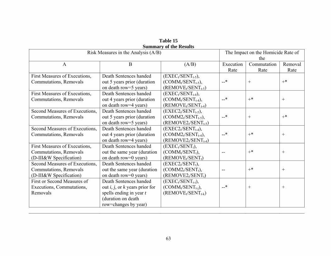
63

Table 15 Summary of the Results

Risk Measures in the Analysis (A/B) The Impact on the Homicide Rate of the

A B (A/B) Execution Rate

Commutation Rate

Removal Rate

First Measures of Executions, Commutations, Removals

Death Sentences handed out 5 years prior (duration on death row=5 years)

(EXECt/SENTt-5), (COMMt/SENTt-5), (REMOVEt/SENTt-5)

--*

+

+*




--*

+*

+

Second Measures of Executions, Commutations, Removals


(EXEC2t/SENTt-5), (COMM2t/SENTt-5), (REMOVE2t/SENTt-5)

--*

+

+*




--*

+*

+

First Measures of Executions, Commutations, Removals (D-III&W Specification)

Death Sentences handed out the same year (duration on death row=0 years)

(EXECt/SENTt), (COMMt/SENTt), (REMOVEt/SENTt)

--

+*

+

Second Measures of Executions, Commutations, Removals (D-III&W Specification)

Death Sentences handed out the same year (duration on death row=0 years)

(EXEC2t/SENTt), (COMM2t/SENTt), (REMOVE2t/SENTt)

--

+*

+

First or Second Measures of Executions, Commutations, Removals

Death Sentences handed out i, j, or k years prior for spells ending in year t (duration on death row=changes by year)

(EXECt/SENTt-i), (COMMt/SENTt-j), (REMOVEt/SENTt-k)

--*

+

+

64


Death Row Inmates (ROW) (EXECt/ROWt), (COMMt/ROWt), (REMOVEt/ROWt)

--*

+*

+


Death Row Inmates (ROW) (EXEC2t/ROWt), (COMM2t/ROWt), (REMOVE2t/ROWt)

--*

+*

+


Total Prisoners (PRIS) (EXECt/PRISt), (COMMt/PRISt), (REMOVEt/PRISt)

--*

+

+


Total Prisoners (PRIS) (EXEC2t/PRISt), (COMM2t/PRISt), (REMOVE2t/PRISt)

--*

+

+

The Raw Count of Executions (#EX), Commutations (#C), Removals (#R)

Population (POP) (#EXt/POPt), (#Ct/POPt), (#Rt/POPt)

--*

+

+


Lagged Murder Rate (MURDER)

(#EXt/MURDERt), (#Ct/MURDERt), (#Rt/MURDERt)

--*

--

+


(#EXt), (#Ct), (#Rt)

--*

--

+

First Measures of Executions, Commutations, Removals (Unweighted Regression)



--*

+*

+*

First Measures of Executions, Commutations, Removals (Unweighted Regression)



--

+*

+*

Second Measures of Executions, Commutations, Removals (Unweighted Regression)



--*

+*

+*

65

Second Measures of Executions, Commutations, Removals (Unweighted Regression)



--

+*

+




--

+

+




--

+

--

A + (--) indicates that the coefficient is positive (negative) in at least 2 of the 3 regressions pertinent to that specification. A * indicates that the coefficient is statistically significant in at least 2 of the 3 specifications. The details are reported in various tables in the paper. Note that a number of specifications summarized in this table are inconsistent with theory. They are estimated and reported here as part of sensitivity analysis. Note also that this table is not an exhaustive summary of the models estimated in the paper. Other models, which are not reported in the interest of space in this table, are consistent with the pattern displayed here. Those results are presented in previous tables.

66

Figure 1A Kansas Homicide Rate

0

1

2

3

4

5

6

7

8

1960 1963 1966 1969 1972 1975 1978 1981 1984 1987 1990 1993 1996 1999 2002

Hom

icid

es p

er 1

00,0

00 P

eopl

e

Figure 2A New Hampshire Homicide Rate

0

0.5

1

1.5

2

2.5

3

3.5

4

1960 1963 1966 1969 1972 1975 1978 1981 1984 1987 1990 1993 1996 1999 2002

Hom

icid

es p

er 1

00,0

00 P

eopl

e

Death Penalty Legal

Death Penalty Legal

67

Figure 3ANew York Homicide Rate

0

2

4

6

8

10

12

14

16

1965 1968 1971 1974 1977 1980 1983 1986 1989 1992 1995 1998 2001 2004

Hom

icid

es p

er 1

00,0

00 P

eopl

e

Figure 4A

New Jersey Homicide Rate

0

1

2

3

4

5

6

7

8

1960 1963 1966 1969 1972 1975 1978 1981 1984 1987 1990 1993 1996 1999 2002

Hom

icid

es p

er 1

00,0

00 P

eopl

e

Death Penalty Legal

Death Penalty Legal

68

Figure 5AMassachusetts Homicide Rate

0

0.5

1

1.5

2

2.5

3

3.5

4

4.5

5

1960 1963 1966 1969 1972 1975 1978 1981 1984 1987 1990 1993 1996 1999 2002

Hom

icid

es p

er 1

00,0

00 P

eopl

e

Figure 6ARhode Island Homicide Rate

0

1

2

3

4

5

6

1960 1963 1966 1969 1972 1975 1978 1981 1984 1987 1990 1993 1996 1999 2002

Hom

icid

es p

er 1

00,0

00 P

eopl

e

Death Penalty Illegal


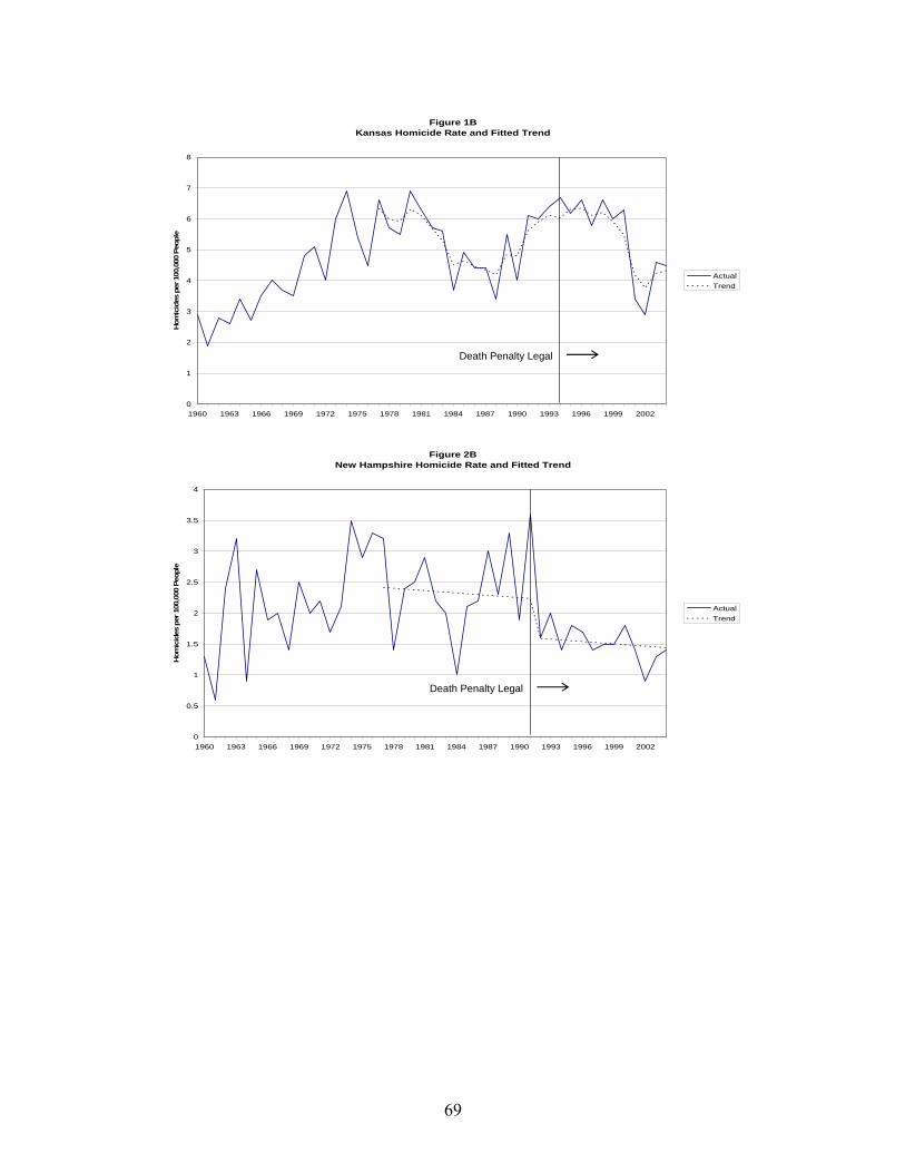
69

Figure 1BKansas Homicide Rate and Fitted Trend

0

1

2

3

4

5

6

7

8

1960 1963 1966 1969 1972 1975 1978 1981 1984 1987 1990 1993 1996 1999 2002

Hom

icid

es p

er 1

00,0

00 P

eopl

e

ActualTrend

Figure 2BNew Hampshire Homicide Rate and Fitted Trend

0

0.5

1

1.5

2

2.5

3

3.5

4

1960 1963 1966 1969 1972 1975 1978 1981 1984 1987 1990 1993 1996 1999 2002

Hom

icid

es p

er 1

00,0

00 P

eopl

e

ActualTrend

Death Penalty Legal

Death Penalty Legal

70

Figure 3BNew York Homicide Rate and Fitted Trend

0

2

4

6

8

10

12

14

16

1960 1963 1966 1969 1972 1975 1978 1981 1984 1987 1990 1993 1996 1999 2002

Hom

icid

es p

er 1

00,0

00 P

eopl

e

ActualTrend

Figure 4B

New Jersey Homicide Rate and Fitted Trend

0

1

2

3

4

5

6

7

8

1960 1963 1966 1969 1972 1975 1978 1981 1984 1987 1990 1993 1996 1999 2002

Hom

icid

es p

er 1

00,0

00 P

eopl

e

ActualTrend

Death Penalty Legal

Death Penalty Legal

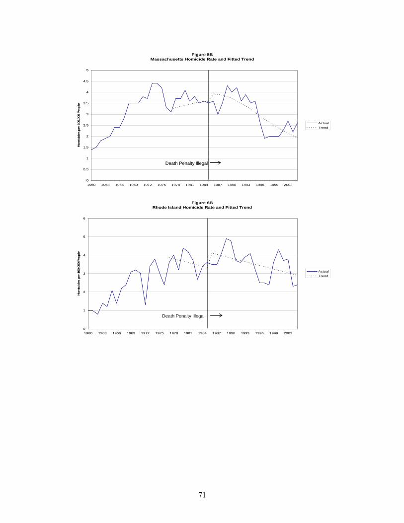
71

Figure 5BMassachusetts Homicide Rate and Fitted Trend

0

0.5

1

1.5

2

2.5

3

3.5

4

4.5

5

1960 1963 1966 1969 1972 1975 1978 1981 1984 1987 1990 1993 1996 1999 2002

Hom

icid

es p

er 1

00,0

00 P

eopl

e

ActualTrend

Figure 6BRhode Island Homicide Rate and Fitted Trend

0

1

2

3

4

5

6

1960 1963 1966 1969 1972 1975 1978 1981 1984 1987 1990 1993 1996 1999 2002

Hom

icid

es p

er 1

00,0

00 P

eopl

e

ActualTrend



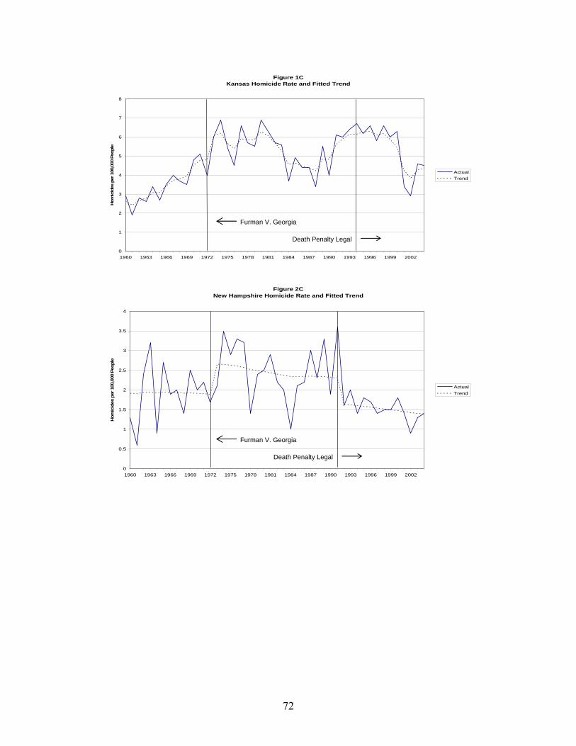
72

Figure 1C Kansas Homicide Rate and Fitted Trend

0

1

2

3

4

5

6

7

8

1960 1963 1966 1969 1972 1975 1978 1981 1984 1987 1990 1993 1996 1999 2002

Hom

icid

es p

er 1

00,0

00 P

eopl

e

ActualTrend

Figure 2CNew Hampshire Homicide Rate and Fitted Trend

0

0.5

1

1.5

2

2.5

3

3.5

4

1960 1963 1966 1969 1972 1975 1978 1981 1984 1987 1990 1993 1996 1999 2002

Hom

icid

es p

er 1

00,0

00 P

eopl

e

ActualTrend

Death Penalty Legal

Death Penalty Legal

Furman V. Georgia

Furman V. Georgia

73

Figure 3CNew York Homicide Rate and Fitted Trend

0

2

4

6

8

10

12

14

16

1960 1963 1966 1969 1972 1975 1978 1981 1984 1987 1990 1993 1996 1999 2002

Hom

icid

es p

er 1

00,0

00 P

eopl

e

ActualTrend

Figure 4C

New Jersey Homicide Rate and Fitted Trend

0

1

2

3

4

5

6

7

8

1960 1963 1966 1969 1972 1975 1978 1981 1984 1987 1990 1993 1996 1999 2002

Hom

icid

es p

er 1

00,0

00 P

eopl

e

ActualTrend

Death Penalty Legal

Furman V. Georgia

Death Penalty legal

Furman V. Georgia

74

Figure 5CMassachusetts Homicide Rate and Fitted Trend

0

0.5

1

1.5

2

2.5

3

3.5

4

4.5

5

1960 1963 1966 1969 1972 1975 1978 1981 1984 1987 1990 1993 1996 1999 2002

Hom

icid

es p

er 1

00,0

00 P

eopl

e

ActualTrend

Figure 6CRhode Island Homicide Rate and Fitted Trend

0

1

2

3

4

5

6

1960 1963 1966 1969 1972 1975 1978 1981 1984 1987 1990 1993 1996 1999 2002

Hom

icid

es p

er 1

00,0

00 P

eopl

e

ActualTrend

Furman V. Georgia

Furman V. Georgia



75

Figure 7CSouth Dakota Homicide Rate and Fitted Trend

0

0.5

1

1.5

2

2.5

3

3.5

4

4.5

1960 1963 1966 1969 1972 1975 1978 1981 1984 1987 1990 1993 1996 1999 2002

Hom

icid

es p

er 1

00,0

00 P

eopl

e

ActualTrend

Figure 8COregon Homicide Rate and Fitted Trend

0

1

2

3

4

5

6

7

1960 1963 1966 1969 1972 1975 1978 1981 1984 1987 1990 1993 1996 1999 2002

Hom

icid

es p

er 1

00,0

00 P

eopl

e

ActualTrend

Death Penalty Legal

Furman V. Georgia

Furman V. Georgia

Death Penalty Legal

76

Figure 9CNew Mexico Homicide Rate and Fitted Trend

0

2

4

6

8

10

12

14

1960 1963 1966 1969 1972 1975 1978 1981 1984 1987 1990 1993 1996 1999 2002

Hom

icid

es p

er 1

00,0

00 P

eopl

e

ActualTrend

Figure 10

Duration on Death Row From Sentencing to Exit

0

2

4

6

8

10

12

14

16

18

1977

1978

1979

1980

1981

1982

1983

1984

1985

1986

1987

1988

1989

1990

1991

1992

1993

1994

1995

1996

1997Ye

ars

on D

eath

Row

Executions Commutations Removals

Furman V. Georgia

Death Penalty Legal

77

References

Argys, Laura M., and Mocan, H. Naci. "Who Shall Live and Who Shall Die? An Analysis of Prisoners on Death Row in the United States" Journal of Legal Studies (2004): 255-92. Ayres, Ian, and Donohue III, John. “The Latest Misfires in Support of the ‘More Guns, Less Crime’ Hypothesis.” Stanford Law Review 55 (2003): 1371-98. Baldus, David C. Woodworth; George, Zuckerman; David, Weiner; Neil Allan; and Broffit, Barbara. “Race Discrimination and the Death Penalty in the Post Furman Era: An Empirical and Legal Overview with Preliminary Findings from Philadelphia.” Cornell Law Review, 83 (1998): 1638-1770. Beccaria, Cesarc, marchese di. On Crimes and Punishment. Indianapolis, Hackett Publishing (1986). Becker, Gary S. “Crime and Punishment: An Economics Perspective.” Journal of Political Economy, 76 (1968): 169-217. Becker, Gary S. Nobel Lecture. http://nobelprize.org/nobel_prizes/economics/ laureates/1992/becker-lecture.html (1992) Becker, Gary, Michael Grossman, and Kevin Murphy. “An Empirical Analysis of Cigarette Addiction.” American Economic Review 81 (1994): 396-418. Bedau, Hugo A. The Death Penalty in America. New York, Oxford University Press, (1982). Bertrand, Marianne; Duflo, Esther; and Mullainathan, Sendhil. “How Much Should We Trust Differences-and-Differences Estimates?” Quarterly Journal of Economics 119 (2004): 249-75. Bentham, Jeremy. A Theory of Legislation. New York, Harcourt, Brace (1931). Bowers, William J. and Pierce, Glenn L. “The Illusion of Deterrence in Isaac Ehrlich’s Research on Capital Punishment.” Yale Law Journal 85 (1975): 187-208. Cameron, Samuel. “A Review of the Econometric Evidence on the Effects of Capital Punishment.” Journal of Socio-Economics 23 (1994): 197-214.

78

Corman, Hope; Noonan, Kelly; Reichman, Nancy; and Dhaval, Dave. “Demand for Illicit Drugs among Pregnant Women.” In Substance Use: Individual Behavior, Social Interactions, Markets and Politics, Bjorn Lindgren and Michael Grossman (eds.). Advances in Health Economics and Health Services Research. Amsterdam, Elsevier, (2005): 41-59.

Corman, Hope, and Mocan, Naci H. “A Time-Series Analysis of Crime, Deterrence, and Drug Abuse in New York City.” American Economic Review 90 (2000): 584-604. Corman, Hope, and Mocan, Naci H. “Carrots, Sticks, and Broken Windows.” Journal of Law and Economics (2005): 235-66. Cover, James Perry and Thistle, Paul D. “Time Series, Homicide, and the Deterrent Effect of Capital Punishment,” Southern Economic Journal 54 (1988): 615-622. Dezhbakhsh, Hashem; Rubin, Paul H.; and Shepherd, Joanna. “Does Capital Punishment Have a Deterrent Effect? New Evidence from Post-moratorium Panel Data.” American Law and Economics Review 5 (2003): 344-76 Dickert-Conlin, Stacey, and Amitabh Chandra, “Taxes and the Timing of Births,” Journal of Political Economy 107 (1999): 161-77. Di Tella, Rafael and Schargrodsk, Ernesto. “Do Police Reduce Crime? Estimates Using the Allocation of Police Forces After a Terrorist Attack,” The American Economic Review 94 (2004): 115-33. Donohue III, John, and Levitt, Steven. “Measurement Error, Legalized Abortion, the Decline in Crime: A Response to Foote and Goetz (2005).” Working Paper No. 11987. Cambridge, MA: National Bureau of Economic Research, 2006. Donohue III, John, and Levitt, Steven. “Further Evidence that Legalized Abortion Lowered Crime: A Reply to Joyce.” Journal of Human Resources 39 (2004): 29-49. Donohue III, John, and Levitt, Steven. “The Impact of Legalized Abortion on Crime” Quarterly Journal of Economics 116 (2001): 379-420. Donohue III, John, and Wolfers, Justin. “Uses and Abuses of Empirical Evidence in the Death Penalty Debate.” Stanford Law Review 58 (2006): 791-846. Ehrlich, Isaac. “The Deterrent Effect of Capital Punishment: A Question of Life and Death.” American Economic Review 65 (1975): 395-417. Ehrlich, Isaac. “Capital Punishment and Deterrence: Some Further Thoughts and Evidence.” Journal of Political Economy 85 (1977): 741-788.

79

Ehrlich, Isaac. “The Deterrent Effect of Capital Punishment: Reply.” American Economic Review 67 (1977): 452-458. Ehrlich, Isaac, and Brower, George D. “On the Issue of Causality in the Economic Model of Crime and Law Enforcement: Some Theoretical Considerations and Experimental Evidence.” American Economic Review 77 (1987): 99-106. Ehrlich, Isaac and Liu, Zhiqiang. “Sensitivity Analyses of the Deterrence Hypothesis: Let’s Keep the Econ in Econometrics.” Journal of Law and Economics 17 (1999): 455-488. Ehrlich, Isaac and Randall, Mark, “Fear of Deterrence: A Critical Evaluation of the “Report of the Panel on Research on Deterrent and Incapacitative Effects” Journal of Legal Studies 6 (1977): 293-316.

Farrell, Susan; Manning, Willard G.; and Finch, Michael D. “Alcohol Dependence and the Price of Alcoholic Beverages,” Journal of Health Economics 22 (2003): 117-47.

Foote, Christopher, and Christopher Goetz. “Testing Economic Hypotheses with State-Level Data: A Comment on Donohue and Levitt (2001).” Federal Reserve Bank of Boston Working Paper, No. 5-15. November 2005.

Forst, Brian. “Capital Punishment and Deterrence: Conflicting Evidence?” Journal of Criminal Law and Criminology 74 (1983): 927-942.

Freeman, Richard B. and Rodgers, William M., III. “Area Economic Conditions and the Labor Market Outcomes of Young Men in the 1990s Expansion.” In Prosperity for All? The Economic Boom and African Americans. Robert Cherry, William M. Rodgers III (eds.). New York, Russell Sage Foundation, (2000): 50-87.

Grossman, Michael. “Individual Behaviours and Substance Use: The Role of Price.” In Substance Use: Individual Behaviour, Social Interactions, Markets and Politics, Bjorn Lindgren and Michael Grossman (eds.). Vol. 16 of Advances in Health Economics and Health Services Research. Amsterdam, Elsevier, 2005; pp. 15-39.

Grossman Michael and Frank Chaloupka. “The Demand for Cocaine by Young Adults: A Rational Addiction Approach.” Journal of Health Economics; 17, (1998); pp, 427-74.

Grossman Michael, Frank Chaloupka, Henry Saffer and A. Laixuthai. “Effects of Alcohol Price Policy on Youth: A Summary of Economic Research.” Journal of Research on Adolescence 4 (1994): 347-64.

Grogger, Jeffrey. “Market Wages and Youth Crime.” Journal of Labor Economics 16 (1998): 756-91.

80

Gruber, Jonathan; Sen, Anindya; and Stabile, Mark. “Estimating price Elasticities when there is Smuggling: The Sensitivity of Smoking to Price in Canada.” Journal of Health Economics 22 (2003): 821-42.

Gruber, Jonathan and Jonathan Zinman. “Youth Smoking in the United States: Evidence and Implications.” In Risky Behavior Among Youths: An Economic Analysis, Jonathan Gruber (ed.) Chicago: The University of Chicago Press (2001): 69-120.

Gould, Eric D.; Weinberg, Bruce A.; Mustard, David B. “Crime Rates and Local Labor Market Opportunities in the United States: 1979-1997.” Review of Economics and Statistics 84 (2002): 45-61 Harbaugh, William T.; Krause, Kate; Liday, Steven G., Jr.; and Vesterlund, Lise. “Trust in Children.” In Trust and reciprocity: Interdisciplinary lessons from experimental research , Ostrom, Elinor; Walker, James (eds.) New York: Russell Sage Foundation (2003): 302-22. Harvey, Andrew, and Durbin, J. “The Effect of Seat Belt Legislation on British Road Causalities: A Case Study in Structural Time Series Modeling.” Journal of the Royal Statistical Society 149 (1986): 187-227. Hoenack, Stephen A., and Weiler, William C. “A Structural Model of Murder Behavior and the Criminal Justice System.” American Economic Review 70 (1980): 327-341. Jacob, Brian A. and Levitt, Steven D. “Rotten Apples: An Investigation of the Pevelance and Predictors of Teacher Cheating.” Quarterly Journal of Economics 118 (2003): 843-877. Joyce, Ted, “Did Legalized Abortion Lower Crime?” Journal of Human Resources 39 (2004a): 1-28. Joyce, Ted, “Further Tests of Abortion and Crime.” Working Paper No. 10564. Cambridge, MA: National Bureau of Economic Research, June 2004b. Katz, Lawrence; Levitt, Steven D.; and Shustorovich, Ellen. “Prison Conditions, Capital Punishment, and Deterrence.” American Law and Economics Review 5 (2003): 318-43. Kipling, Rudyard. From Sea to Sea: vol. 9 New York, Doubleday & Co. (1914). Kleck, Gary. “Racial Discrimination in Criminal Sentencing: A Critical Evaluation of the Evidence with Additional Evidence on the Death Penalty.” American Sociological Review 46 (1981): 783-804. Kessler, Daniel P., and Levitt, Steven D. “Using Sentence Enhancements to Distinguish between Deterrence and Incapacitation.” Journal of Law and Economics 42 (1999): 343-63.

81

Layson, Stephen K. “Another View of the Canadian Time-Series Evidence on Homicide and Deterrence.” Canadian Journal of Economics 16(1983): 52-73. Leamer, Edward. “Let’s Take the Con out of Econometrics,” American Economic Review 73 (1983): 31-43. Levitt, Steven D. “The Effect of Prison Population Size on Crime Rates: Evidence from Prison Overcrowding Litigation." The Quarterly Journal of Economics, 111(2), (1996) pp. 319-51. Levitt, Steven D. “Using Electoral Cycles in Police Hiring to Estimate the Effect of Police on Crime,” American Economic Review 87 (1997): 270-290. Levitt, Stephen D. “Juvenile Crime and Punishment,” The Journal of Political Economy 106 (1998a): 1156-1185. Levitt, Stephen D. “Why Do Increased Arrest Rates Appear to Reduce Crime: Deterrence, Incapacitation, or Measurement Error?” Economic Inquiry 36 (1998b): 353-372. Lott, John R. Jr. and Mustard, David B. “Crime, Deterrence, and Right-to-Carry Concealed Handguns.” The Journal of Legal Studies 26 (1997): 1-68.

Lundberg, Shelly and Plotnick, Robert D. "Effects of State Welfare, Abortion and Family Planning Policies on Premarital Childbearing among White Adolescents.” Family Planning Perspectives 22 (1990): 251-75.

Lundberg, Shelly and Plotnick, Robert D. "Adolescent Premarital Childbearing: Do Economic Incentives Matter?" Journal of Labor Economics 13 (1995): 177-200.

Manning, Willard G., Blumberg, L.; and Moulton, L. “The Demand for Alcohol: The Differential Response to Price.” Journal of Health Economics 14 (1995): 123-48.

McFarland, Sam G. “Is Capital Punishment a Short-Term Deterrent to Homicide? A Study of the Effects of Four Recent American Executions.” Journal of Criminal Law and Criminology 74 (1983): 1014-1032. McManus, Walter S. “Estimates of the Deterrent Effect of Capital Punishment: The Importance of the Researcher’s Prior Beliefs.” Journal of Political Economy 93 (1985): 417-425.

Mellor, Jennifer M. "The Effect of Family Planning Programs on the Fertility of Welfare Recipients: Evidence from Medicaid Claims." Journal of Human Resources 33 (1998): 866-95.

82

Mocan, Naci. "Is There a Unit Root in U.S. Real GNP? A Re-Assessment." Economics Letters 45 (1994): 23-31.

Mocan, Naci, and Gittings, Kaj R. “Getting Off Death Row: Commuted Sentences and the Deterrent Effect of Capital Punishment.” Journal of Law and Economics 46 (2003): 453-478.

Mocan, Naci and Rees, Daniel. “Economic Conditions, Deterrence and Juvenile Crime: Evidence from Micro Data.” American Law and Economics Review 7 (2005): 319-49. Mocan, Naci, and Topyan, Kudret. “Real Wages over the Business Cycle: Evidence from a Structural Time-Series Model." Oxford Bulletin of Economics and Statistics 55 (1993): 363-89. Moody, Carlisle. “Testing for the Effects of the Concealed Weapons Laws: Specification Errors and Robustness.” Journal of Law and Economics 44 (2001): 799-813. Mustard, David B. “Reexamining Criminal Behavior: The Importance of Omitted Variable Bias.” Review of Economics and Statistics 85 (2003): 205-11.

Pacula, Rosalie, Michael Grossman, Frank Chaloupka, Patrick O’Malley, Llyod Johnston and Matthew Farrelly. “Marijuana and Youth.” In Risky Behavior Among Youths: An Economic Analysis, Jonathan Gruber (ed.) Chicago: The University of Chicago Press, (2001): 271-326.

Passell, Peter and Taylor, John. “The Deterrent Effect of Capital Punishment: Another View.” American Economic Review 67 (1977): 445-451. Plassmann, Florenz, and Tideman, Nicolaus. “Does the Right to Carry Concealed Handguns Deter Countable Crimes? Only a Coumt Analysis Can Say.” Journal of Law and Economics 44 (2001): 771-98. Plassmann, Florenz, and Whitley, John. “Confirming ‘More Guns, Less Crime.’ ” Stanford Law Review 55 (2003): 1313-69. Pokorak, J. “Probing the Capital Prosecutor’s Perspective: Race and Gender of the Discretionary Actors.” Cornell Law Review 83 (1998): Raphael, Steven and Winter-Ebmer, Rudolf. ” Identifying the Effect of Unemployment on Crime,” The Journal of Law and Economics XLIV (2001): 259-83. Saffer, Henry and Dave, Dhaval. “Mental Illness and The Demand for Alcohol, Cocaine and Cigarettes.” Economic Inquiry 43 (2005): 229-46. Saffer, Henry, and Chaloupka, Frank. “The Demand for Illicit Drugs.” Economic Inquiry 37 (1999): 401-11.

83

Sorensen, Jon; Wrinkle, Robert; Brewer, Victoria, et. al. “Capital Punishment and Deterrence: Examining the Effect of Executions on Murder in Texas.” Crime and Delinquency 45 (1999): 481-493. Sunstein, Cass and Vermeule, Adrian. “Deterring Murder: A Reply.” Stanford Law Review 58 (2006): 847-57.

Van Ours, Jan. “The Price Elasticity of Hard Drugs: The case of Opium in the Dutch East Indies, 1923-1938.” Journal of Political Economy103 (1995): 261-79.

Yurekli A. and P. Zhang, “The Impact of Clean-air laws and Cigarette Smuggling on Demand for Cigarettes: An Empirical Model.” Journal of Health Economics 9 (2000): 159-70.

the impact of incentives on human behavior: can we …

Documents