The Impact of Homework Time on Academic Achievement

Steven McMullen∗

The University of North Carolina at Chapel Hill

October 2007

Abstract

This paper demonstrates that the amount of time students spend on homework

plays a central role in determining academic success. A policy investment which takes

advantage of this fact can do more to increase academic achievement than similar

investments in traditional policy options such as decreasing class size or increasing

teachers’ wages. This study uses longitudinal data on students, teachers and school

characteristics to estimate the impact of homework time, and the impact of the amount of

homework assigned, on mathematics achievement. Previous studies have not been able

to accurately estimate the impact of homework because of important omitted variables

and measurement error, which strongly bias the estimated impact of homework time.

This paper, however, uses an instrumental variable estimate with student fixed effects to

account for both time-varying and time-invariant unobserved characteristics and inputs.

This technique produces estimates of the impact of homework time on academic

achievement that are much higher than those of previous studies. Moreover, these

findings suggest that a policy change of assigning extra homework each week primarily

improves the achievement of low performing students and students in low performing

schools. This suggests a possible policy solution to the gap in achievement between high

and low performing students.

∗ The author would like to thank Tom Mroz, David Blau, Donna Gilleskie, David Guilkey, and Helen Tauchen for their excellent assistance. Steven can be reached at mcmullen@unc.edu or Department of Economics, Gardner Hall CB# 3305, University of North Carolina, Chapel Hill, NC 27599-3305.

2

I. Introduction

In a recent international comparison of the amount of time that students spend on

homework, students from the United States ranked near the bottom of the 20 countries

surveyed (Harmon et al. 1997). Furthermore, research indicates that over the last 25

years high school students have decreased the amount of homework that they complete

(Brookings Institution 2003). Nonetheless, there is a popular conception that students are

being assigned too much homework.1 One key empirical question that underlies the

homework debate is how much benefit students receive from time spent studying.

Despite much research on the topic, accurate measurements of the return to homework

have not been forthcoming. Scholars that have approached this topic have done little to

control for the endogeneity arising because of omitted variables that likely have a large

influence on students’ choices regarding study time.2

In this paper, I estimate two effects. First this paper estimates impact that

students’ time spent doing homework has on achievement test scores. Second, I examine

the impact of assigning additional homework on achievement. The primary challenge

that this study overcomes is that there are likely a host of unobserved variables that

influence both how much time a student spends on homework and the students’

achievement test scores. By combining instrumental variables estimation with an

individual-fixed-effects specification, I control for both unobserved heterogeneity that is

1 The Brookings Institution press release (2003) writes that “Since 2001, feature stories about onerous homework loads and parents fighting back have appeared in Time, Newsweek, and People magazines; the New York Times, Washington Post, Los Angeles Times, Raleigh News and Observer, and the Tampa Tribune; and the CBS Evening News and other media outlets.” Their research indicates that the homework load for most US students is actually quite low. 2 Recent work done by economists such as Aksoy and Link (2000), and Stinebrickner and Stinebrickner (2007) have made progress, but their approaches can only address a subset of the endogeneity problems involved with measuring this effect.

3

constant over time and time-varying heterogeneity that might influence the amount of

time students spend on homework. This approach yields estimates of the impact of

homework that are much larger than those of previous studies. The presence of time-

varying unobserved factors is especially important to consider when estimating the

impact of education inputs that are under the students’ control, since students can respond

in each period to changing incentives.

I find that one extra hour of mathematics homework per week improves

mathematics achievement by 0.243 standard deviations. This change is large enough to

move a student from the 50th percentile of math achievement to 59th percentile over the

course of a school year. Additionally, this effect varies based on student characteristics

and institutional factors. I find evidence that low achieving students and those in lower-

performing schools realize much higher returns to their homework time than other

students. Likewise, a policy of assigning more homework disproportionately benefits

these students. These findings lead to two important conclusions. First, that it is possible

for students to overcome past poor performance or a low quality school by spending more

time doing homework. Second, that a policy that increases the amount of homework

assigned is likely to reduce the gap between low and high achieving students.

Finally, in order to compare policy instruments, I estimate the cost-effectiveness

of increasing student achievement by assigning more homework, decreasing class size,

and increasing teachers’ salaries. For a given monetary investment, increasing the

amount of assigned homework improves achievement almost three times as much as

increasing teachers’ wages, and eleven times as much as decreasing class size.

4

II. Background

Previous studies within the education production function literature have

documented a number of inputs that have an impact on students’ academic achievement.

These include school funding (Altonji and Dunn 1996), class size,3 teacher characteristics

and training (Hanushek, et al 1998; Hanushek and Rivkin 2007), the amount of time

spent in class or in school (Aksoy and Link 2000), and the performance of a student’s

peers (Sacerdote 2001; Zimmerman 2003; Hanushek and Rivkin 2006). Certain

characteristics of the student and their family also are important, including parents’

permanent income (Blau 1999; Dahl and Lochner 2005) as well as the student’s race and

sex.

The focus of this study will be on another input: student time spent on homework.

The theoretic literature predicts a positive impact of homework time on academic

achievement (Betts 1996; Neilson 2005). Almost all of the empirical studies on this topic

conclude that homework time has a positive impact on academic achievement, although

there is no consensus on the magnitude of the impact. The literature pertaining to this

topic will be presented in two sections: first, a review of literature from outside the

economics discipline, and second, a review of recent work done by applied economists.

Within the fields of education, psychology, and sociology there has been much

research on the impact of homework. Cooper et al. (2006) provides a good review of

recent work in these fields. All of the published studies that Cooper et al. review that use

multivariate regression analysis find similar results: increased homework causes a small

increase in academic achievement. These studies, however, are limited to cross section

3 Decreasing class size has a small impact, except in early grades. For a review of the class size literature, see Hanushek (1998).

5

analysis and do not try to take into account omitted inputs or characteristics. Shuman et

al. (1985), Hill (1991), and Rau and Durand (2000) all find similar results when trying to

document the impact of homework time on the performance of college students. Each

study either finds the relationship hard to document or finds a small effect of homework

time on college grades.

Applied economists have only recently started to pay attention to the impact of

homework time on achievement, starting with Julian Betts’ 1996 analysis of the

Longitudinal Study of American Youth. Since then Aksoy and Link (2000), Eren and

Henderson (2007), and Stinebrickner and Stinebrickner (2007) have all examined this

question. Each of these studies makes a serious attempt to address unobserved inputs.

Eren and Henderson, in the parametric portion of their paper, use a value added

specification,4 both Betts and Aksoy and Link use a specification with student fixed

effects, and Stinebrickner and Stinebrickner use the students’ roommate’s videogame

ownership as an instrument, estimating the effect with two stage least squares.

Relative to this past work, this study improves the estimation of the effect of

homework on academic achievement in two ways. First, the primary shortcoming in this

literature is that previous work fails to adequately account for unobserved inputs that

influence both academic achievement and the amount of time spent on homework. None

of these studies, with the exception of Stinebrickner and Stinebrickner5 can account for

unobserved influences that vary over time. To address this potential problem I use the

4 The value added specification is a cross section regression with a lagged test score (or other dependent variable) included on the right hand side of the equation to control for past achievement, inputs, and student characteristics. 5 Stinebrickner and Stinebrickner (2007) does a good job documenting the relationship between homework and achievement, but does so within a selected non-representative college age population. Their instrumental variable strategy, however, is not reproducible on a large scale.

6

amount of assigned homework and the student’s locus of control as instruments for

student homework time, as well as a student fixed effects. Dealing with the endogeneity

of students’ homework time in this manner greatly influences the estimated effects.

Second, previous research has documented that the return to homework time varies based

on a student’s ability (Eren and Henderson 2007). In this study, I also document that the

return to homework also varies with school quality. Finally, this paper documents that a

policy of increasing the amount of homework assigned to students is a cost-effective

alternative to traditional policy interventions, and that this policy would

disproportionately aid low-performing students and those in low-performing schools.

III. A Model of Homework Time Allocation and Academic Achievement

This section presents a brief descriptive model describing the relationship

between students’ time allocation choices, the education production function, and

external labor market signals. This framework will be used in the next section to

motivate an econometric strategy. First, student i at time t maximizes expected present

discounted utility Uit, which depends on leisure time (Di-Hit), future expected income (Ii),

and individual/family characteristics and preferences (Xit), where Di is the disposable

time available to the student to allocate between homework time (Hit) and leisure. The

utility function also includes a set of inputs (Zit), that influence utility through interaction

with the amount of homework that students do.

(1) ( , , , )it i it i it itU u D H I X Z= −

The student chooses to invest in homework time in order to increase their human capital

(Eit) which is also a function of previous human capital (Eit-1), innate ability (Ai), school

7

and district inputs (Sit), teacher inputs (Tit), individual characteristics (Xit), and a shock

( itυ ) that might include an external event (illness, divorce) or the chance of getting placed

in a class which proves exceptionally difficult or easy for other reasons.

(2) ( )1, , , , , ,it it it i it it it itE f E H A S T X υ−=

This education production function, f, will dictate the return (in terms of academic

achievement) of an hour of homework, which can vary by student ability, school quality,

and other characteristics.

Education pays off by increasing the future income, which is also a function of

ability, labor market characteristics (Lt), and whether or not the student chooses to go to

college.

(3) ( ), , ,i iT i T iI g E A L C=

The optimal amount of homework can vary across students, and will be a function h of

prior education, ability, school inputs, teacher inputs, the labor market, and individual

characteristics. Homework will also vary based a set of individual characteristics and

school policies (Zit) that do not independently enter into the education production

function. These can be personal characteristics that have no influence on academic

performance, institutional characteristics that alter students’ incentives to study, or other

environmental factors.

(4) *

1( , , , , , , , )it i it it t it it it itH h A S T L E X Zυ−=

Even within a class students will vary in the amount of homework that they do because

different levels of ability may impact the productivity of the time spent on homework,

8

differing levels of past achievement, different preferences, and because they realize

different shocks to their education which may induce them to study more or less often.

IV. Empirical Approach & Identification

Using the framework from the previous section, this section will summarize the

challenge of identifying the parameters of the education production function f (equation

2), and explain the econometric approach for overcoming these challenges.6 The simplest

approach would be to estimate the following linear cross sectional econometric model:

(5) 0 1 2 3 4 5 6 1

U U U

it it it it it i it it itAT H S T X A Eα α α α α α α υ ε−= + + + + + + + +

Where ATit is an achievement test score, which serves as a measure of human capital

(Eit), the alpha parameters represent the impact of the inputs on academic achievement,

and itε is an error term. The superscript U indicates variables that are not observed, and

are part of the residual. Estimating this model will most likely produce biased estimates

of the impact of homework (the parameter 1α ) for three reasons:

1. The input Hit is partially determined by the student ability (Ai) and previous

human capital investments (Eit-1), which also impact the students’ achievement.

These inputs are unobserved, however, and their impact on student study time is

uncertain.

2. The unobserved human capital shock itυ likely biases the parameter estimate

downward, since a negative shock to a students’ education would likely both

6 For a more general discussion of the identification of education production function parameters see Todd and Wolpin 2003.

9

decrease the amount the student learns in the year and increase the amount of time

spent on homework (Stinebrickner and Stinebrickner 2007).7

3. The amount of homework that students complete is measured with some error.

This variable is recorded categorically, and the questions and categories change

slightly across waves. Measurement error of this type could bias the parameter

estimate downward.

Because the magnitude of these impacts is unknown, and there are possible biases in each

direction, it is unclear whether the OLS cross section estimates will be biased upward or

downward.

One method for addressing these identification problems is the use of

instrumental variables estimation. This approach uses one or more Zit variables which

must be good predictors of student homework and be uncorrelated with the omitted

variables. These instruments are used, along with any other exogenous inputs in the

education production function, to predict student homework time. This isolates the

variation in homework time that is not correlated with the omitted variables. Estimating

the effect of this exogenous variation in homework on achievement gives a consistent

estimate of the impact of homework.

First, the amount of time spent on homework is estimated using ordinary least

squares, as shown in equation (6):

(6) 0 1 2 3 4 5it it it it it it itH Z S T X Lβ β β β β β ϕ= + + + + + +

7 For example, if a student became seriously ill for one semester, their test scores would likely suffer, but at the same time, they might increase the amount of time spent on homework in an attempt to make up for missed school. This would create a spurious negative correlation between homework time and test scores. A similar process may be likely for other types of shocks to a students’ education, such as an poor teacher-student match. For a larger discussion of this effect, see Stinebrickner and Stinebrickner 2007.

10

In this specification, the school inputs, teacher inputs and observed student characteristics

are assumed to be exogenously determined. The second step is to estimate the education

production function as shown in equation (7), using the amount of homework predicted

by the estimation of equation (6) ( ˆitH ) instead of the observed homework amount (Hit).

(7) 0 1 2 3 4 5 6 1ˆ U U U

it it it it it i it it itAT H S T X A Eα α α α α α α υ φ−= + + + + + + + +

The omitted variables (Ai, Eit-1, itυ ) are still present in the residual of equation (7), but

they will not be correlated with the predicted homework variable ( ˆitH ).

The instrumental variables approach may not produce a consistent estimate of the

impact of homework if there are more endogenous variables besides the homework

variable. If the omitted variables are also correlated with the other inputs in the education

production function, then including these other inputs can bias the estimate of the effect

of homework ( 1α ). A fixed effects estimator (or within estimator) can be useful for

eliminating certain types of omitted variables problems. To illustrate this, assume that

the observed value of each variable can be decomposed as follows: H

it i it itH H H σ= + +ɶ ,

where iH is permanent homework, or the average value of the homework variable across

time for student i, itHɶ is transitory homework, defined as the deviation from the student’s

permanent homework for that year, and H

itσ is measurement error in the homework

variable. Rewriting equation (5), and suppressing the measurement error term for all

except the homework variable gives us equation (8):

(8) ( ) ( ) ( ) ( )

~

0 1 2 3 4

5 6 1

H

i it i it it i it i it i it

U U U

i it it it

AT AT H H S S T T X X

A E

α α σ α α α

α α υ ε−

+ = + + + + + + + + + +

+ + + +

ɶɶ ɶ ɶ

11

The inclusion of student fixed effects in the OLS specification, as shown in equation (9),

will control for the impact of the permanent component of each input.

(9) ( )~

1 2 3 4

H Uit i it it it it it it itAT H S T Xγ α σ α α α υ η= + + + + + + +ɶɶ ɶ ɶ

This will eliminate bias caused by omitted variables under certain conditions. First, the

omitted variables must not change over time. Second, the relationship between the

omitted variables and achievement must be linear. Third, the permanent component of

each variable may be correlated with the omitted variables, but the transitory component

must not be. Thus even if there are multiple endogenous inputs in the education

production function, the bias from time-invariant omitted variables, such as student

ability (Ai) and previous education investments (Eit-1), will be eliminated. Moreover, if

the other inputs, such as teacher experience, certification, wages, or class size, are

selected by students and parents, this selection is likely based on permanent student

characteristics. So any bias caused by self selection is likely eliminated by using student

fixed effects.

The impact of homework parameter ( 1α ) will be the same in equation (9) and in

equation (5) only if the marginal impact of a change in permanent homework is equal to

the marginal impact of a change in transitory homework. The research of Cunha et al.

(2007) suggests, however, that at least for large changes in education inputs, that this

assumption is unrealistic. Their conclusion is that the transitory effect that is measured in

this paper is likely to be somewhat smaller than the cumulative impact of a permanent

change in student homework time.

12

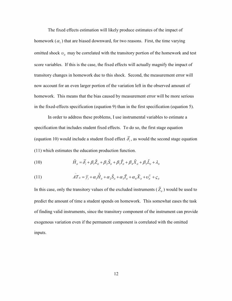
The fixed effects estimation will likely produce estimates of the impact of

homework ( 1α ) that are biased downward, for two reasons. First, the time varying

omitted shock itυ may be correlated with the transitory portion of the homework and test

score variables. If this is the case, the fixed effects will actually magnify the impact of

transitory changes in homework due to this shock. Second, the measurement error will

now account for an even larger portion of the variation left in the observed amount of

homework. This means that the bias caused by measurement error will be more serious

in the fixed-effects specification (equation 9) than in the first specification (equation 5).

In order to address these problems, I use instrumental variables to estimate a

specification that includes student fixed effects. To do so, the first stage equation

(equation 10) would include a student fixed effect iδ , as would the second stage equation

(11) which estimates the education production function.

(10) 1 2 3 4 5it i it it it it it itH Z S T X Lδ β β β β β λ= + + + + + +ɶɶ ɶ ɶ ɶ ɶ

(11) ~

1 2 3 4

ˆ Uit i it it it it it itAT H S T Xγ α α α α υ ς= + + + + + +ɶɶ ɶ ɶ

In this case, only the transitory values of the excluded instruments ( itZɶ ) would be used to

predict the amount of time a student spends on homework. This somewhat eases the task

of finding valid instruments, since the transitory component of the instrument can provide

exogenous variation even if the permanent component is correlated with the omitted

inputs.

13

Instruments

The two variables used in this study as instruments are the amount of homework

assigned by the student’s teacher, and the student’s measured locus of control. The

amount of homework assigned by the student’s instructor is unlikely to have any direct

causal impact on test scores, except in the case that the student actually completes the

homework assignment. This variable may reflect the ability and motivation of the

students, however, if teachers assign more homework to classes with gifted or more

motivated students, such as advanced placement or honors courses. For this reason, this

variable may not be a valid instrument, except when student fixed effects are included in

the first stage regression. The fixed effects will control for any selection based on time-

invariant characteristics, such as student ability. These exogeneity of the instruments is

tested in section six.

The second variable that is used to predict students’ homework is the locus of

control. This variable measures the degree to which a student believes that they can

impact their own future, and varies greatly within students over time. A student with an

internal locus is more likely to believe that their future depends on choices that they

make, while a student with an external locus is more likely to believe that external forces

will dictate the events of their life.8 Previous studies have correlated a strong internal

locus of control with positive outcomes in situations that require independent decision-

making, such as positive health behaviors (Steptoe and Wardle 2001), lower dropout rates

in distance education (Parker 1999) and success in web-based coursework (Wang and

8 The locus of control used here is a combination of students’ answers to three standard questions which ask the student things which might influence their future. For a detailed description of the construction of the locus of control variable, see appendix A.

14

Newlin 2000). Students with an internal locus, on average, spend more time doing

homework, since they are more likely to expect the time investment today to pay off in

the future. While this characteristic predicts the amount of time spent on homework, it

does not, in a fixed effects specification, separately predict achievement test scores.

V. Data

The primary data used for the empirical work is the National Education

Longitudinal Study of 1988, a nationally representative longitudinal survey of students

who were in the 8th grade in 1988. Follow up surveys were given in 1990 and 1992, with

teacher and school counselor surveys in each wave, and parent surveys in the first and

third waves. With each survey the students were given achievement exams in

mathematics, science, English, and history. The exams are designed to allow comparison

across waves, and to accurately test students at different achievement levels. Of the

17,580 students who have at least two recorded mathematics exam scores, 2295 students

were not included in the sample used here because they did not respond to the questions

about homework time or locus of control. 5928 students were not included because the

students’ teachers did not respond to questions about their class size, experience or

assigned homework, and 1455 were not included because of missing data on teachers’

wages or the student’s peers’ behavior. The resulting sample includes 17610

observations on 7902 students. The characteristics of these students do not differ

substantially from the general sample. Summary statistics of the variables used in this

paper are shown in table 1.

15

Mean Std. Dev. Mean Std. Dev. Mean Std. Dev.

Hours of Mathematics Homework 1.46 1.68 5.31 4.74 5.76 4.27

Hours of Assigned Homework 2.23 0.95 3.21 1.79 2.88 1.41

Mathematics Test Score 4.68 0.83 5.21 0.95 5.87 0.96

Class Size 24.06 5.12 23.50 5.53 27.76 16.62

Teachers are Certified in Subject Matter 0.82 0.37 0.99 0.08 0.99 0.10

Inexperienced Teachers 0.10 0.22 0.11 0.22 0.07 0.25

Minimum Teacher Wage 28.48 5.18 29.40 5.60 30.92 6.64

Locus of Control 0.09 0.58 0.06 0.61 0.14 0.62

Average Peers' Test Score 5.34 0.52 5.49 0.68 5.65 0.73

Average Peers' HW Time 5.43 1.72 7.46 2.29 13.14 3.37

State Unemployment Rate 5.70 1.54 5.60 0.98 7.22 1.41

Minimum Wage 3.37 0.07 3.50 0.29 4.27 0.08

Industry Mix 8.05 0.16 8.08 0.17 8.09 0.16

State Public four year tuition 1.61 0.53 1.92 0.67 2.43 0.82

State Financial Aid Per Student 0.33 0.27 0.36 0.28 0.46 0.39

State Higher Ed. Appropriations Per Student 6.39 1.88 6.90 2.05 6.74 1.64

Number of Students 7450 6402 3758

This Data is from the National Education Longitudinal Study of 1988. Wave 1 corresponds to students in the

8th grade, wave 2 to the 10th grade, and wave 3 to the 12th grade. The summary statistics for this sample do

not differ substantially from the complete sample of collected data. All monetary variables are measured in

thousands of dollars, and inflation adjusted to 2005 dollars.

Wave 1 Wave 2 Wave 3

Table 1: Summary Statistics

In addition to the NELS data, data on state minimum wage laws from the

department of labor is added, as is industry mix data from the 1988, 1990, and 1992

IPUMS Current Population Survey March supplement. The state level unemployment

rate data came from Bureau of Labor Statistics. These data sets are used to create the

labor market variables, which are merged with the NELS by the students’ state of

residence. Finally, the higher education variables come from the Almanac of Higher

Education (1989-1994). For variable definitions, see appendix A.

VI. Results

The Impact of Mathematics Homework on Mathematics Achievement

16

Table 2 displays estimates from a series of estimation techniques and

specifications.9 Each specification includes wave indicator variables, the average

observed class size and three indicators of teacher quality: whether the student’s teachers

are certified in their subject, an indicator that the teacher has less than 4 years of

1 2 3 4 5 6 7

Estimation Method OLS 2SLS OLS 2SLS 2SLS 2SLS 2SLS

0.036 0.839 0.006 0.221 0.222 0.244 0.243

(0.002) (0.084) (0.001) (0.072) (0.074) (0.087) (0.086)

-0.003 -0.001 -0.001 0.000 0.000 0.000 0.000

(0.001) (0.003) (0.000) (0.001) (0.001) (0.001) (0.001)

0.126 -0.070 -0.011 -0.014 -0.014 -0.002 -0.001

(0.026) (0.057) (0.014) (0.034) (0.034) (0.037) (0.037)

-0.237 0.091 -0.016 0.090 0.099 0.108 0.106

(0.029) (0.102) (0.015) (0.051) (0.052) (0.059) (0.058)

0.006 0.025 0.003 0.009 0.007 0.005 0.004

(0.002) (0.005) (0.001) (0.003) (0.003) (0.003) (0.003)

Student Fixed Effects no no yes yes yes yes yes

Peer Effects no no no no yes yes yes

Labor Market Characteristics no no no no no yes yes

Higher Edu. Market Characteristics no no no no no no yes

Sargan Statistic (Chi-Sq p-value) n/a 0.253 n/a 0.655 0.608 0.694 0.679

Standard errors are shown in parentheses. The dependent variable for each regression is the mathematics

achievement test score. All regressions include wave indicators. The sample includes 17610 observations

on 7902 students. Columns one and two are pooled regressions with the standard errors clustered at the

level of the individual. The first stage regressions are shown in table 3.

Table 2: Education Production Function Estimation Results

Hours of Math Homework

Class Size

Minimum Teacher pay

Certified Teacher

Inexperienced Teacher

experience, and the minimum teacher pay in the student’s school. The ordinary least

squares estimate of the impact of an hour of mathematics homework per week, shown in

column one, is a 0.036 standard deviation increase in the student’s mathematics test

score, which corresponds to an improvement of about 1.5 percentile points.10 This

estimate is most likely biased if the students’ unobserved prior education inputs or innate

abilities influence the amount of time spent on homework. Column two shows the

instrumental variables estimates from the second stage equation of the same specification

9 For the full results for the main specifications, see appendix B. 10 Starting from the 50th percentile in Mathematics test scores within the sample.

17

as that of column one. The amount of homework assigned and the student’s locus of

control are used as instruments excluded from the second stage to identify the amount of

homework that students complete. The instrumental variables estimate is twenty-three

times higher that the estimate from column one, at 0.839 achievement test standard

deviations, or and improvement 29 percentile points for each hour of homework. This

estimate is likely much higher for three reasons. First, it corrects for the downward bias

due to measurement error. Second, it corrects for the downward bias documented by

Stinebrickner and Stinebrickner (2007) that results from students responding to education

shocks. Third, the two stage least squares estimate could be biased upward if students

with greater motivation or intelligence select more difficult courses that include more

assigned homework, since the amount of homework assigned is being used as an

instrument. I test the validity of the instruments later, and find that in this specification,

the estimate of the impact of homework is likely biased upward due to selection of this

type.

The instrumental variables estimate may also be biased if students select other

inputs based on unobservable characteristics. For example, parents of more able children

may select better school districts with smaller class sizes and more qualified teachers. If

this is the case, the other endogenous inputs can bias the estimate of the impact of an

extra hour of homework.

In order to control for these selection issues, a fixed effects specification is

employed. If the selection is based on student characteristics that do not change over

time, then the student-fixed effects estimate will eliminate the bias not only in the impact

of hours of homework, but also in the other inputs. This estimator will also control for

18

the linear effects of any differences in past inputs that are not included in these

specifications. The third column in table 2 shows the estimates of the same specification

as the one shown in the first column, but with student fixed effects included. These

estimates are much smaller. The impact of an hour of homework with student fixed

effects is 1/6th the size of the OLS estimates presented in the first column.

The fixed effects estimate, however, is likely biased downward for a couple of

reasons. First, as discussed in section four, any problems with measurement error can be

magnified by including student fixed effects.11 Second, Stinebrickner and Stinebrickner

(2007) demonstrate that students respond to negative education shocks by spending more

time on homework. This means that if a student becomes ill one semester they may

increase their homework time. If this is the case, it could cause the OLS estimates of the

impact of homework to be biased downward. The fixed effects estimate will magnify

this bias as well.

The problems with the fixed effects estimates can be addressed by using

instrumental variables in addition to the student fixed effects. The fourth column in table

2 shows the results of the student fixed effects specification estimated using two-stage

least squares, where the excluded instruments are again the amount of homework

assigned by the student’s teachers and the student’s locus of control. This estimate, while

less precisely estimated than the fixed-effects estimate, is much higher, and gives a

quantitatively and qualitatively different result. A student who completes an extra hour

of homework each week is estimated to improve their mathematics test score by 0.22

11 The hours of homework variable is measured with some error: the question given to students is asked slightly differently in each wave, and is coded categorically. Students are assigned the mean value of each category range.

19

standard deviations, an improvement of 8 percentile points for each hour studied. A

standard deviation increase in mathematics homework time, roughly 4 hours per week,

would increase the student’s mathematics test score by 30 percentile points. Even if we

accept the lower bound of the 95% confidence interval for this estimate, which is 0.079

standard deviations, the return to homework is still 13 times higher than the fixed effects

estimate. This lower bound estimate indicates that an hour of homework per week would

move a student from the 50th percentile to the 53rd percentile in mathematics

achievement.

If the instruments provide exogenous variation in student homework time, the

estimates in the fourth column should not change substantially when other inputs are

included in the specification. Columns five through seven test this by adding a series of

other factors which might influence homework time. In each case the estimate of the

return to homework changes only a small amount.

First, in order to control for other school-wide inputs and peer group influences,

the specification shown in column five includes the average amount of homework done

by the students’ peers,12 and the average mathematics test score of the student’s peers.13

The estimate of the impact of homework remains almost exactly the same.

Second, in column six, four state level labor market variables are added to the

specification: the unemployment rate, the unemployment rate squared, the minimum

wage, and an industry mix index that categorizes industries based on the average

12 The students peers, in this case, are any students with observed test scores from the same school in the same year. 13 Manski (1993) and Hanushek et. al. (2003) argue that peer effects of this type can introduce a bias due to the reintroduction of a student’s ability through the student’s influence on her peers. The estimated impact of homework does not change when these variables are included, indicating that if these variables are problematic, they do not bias the estimate of the impact of homework.

20

education level of their workers. These variables have been shown to be important

predictors of student homework time (McMullen 2007). Moreover, column seven adds

three higher education characteristics: the average tuition in four-year public institutions

by state, the financial aid per college student by state, and state-level higher education

appropriations per student. The combined impact of the labor market and college market

variables is a small increase in the estimated impact of homework, indicating that

controlling for external economic influences does not substantially impact the estimate of

the return to homework.

In the final specification, shown in the seventh column, one hour of homework is

estimated to increase as student’s mathematics test score by 0.241 standard deviations, or

nine percentile points. Four additional hours of math homework per week, a little over a

standard deviation change, could move a student from the 50th percentile in mathematics

to the 82nd percentile.

This estimate is especially large when considered in the context of the literature

on school inputs. Cunha et al. (2007) demonstrate that inputs into the education

production function are best considered as cumulative investments, with strong

diminishing returns in any one period. The effect estimated in this paper, however, is a

transitory effect. The best interpretation of these estimates is that they measure the

impact of an additional hour of homework in one period only. If a student devotes extra

time to homework each year over the course of their high school career, however, the

cumulative result on achievement is likely to be larger than the sum of these transitory

effects.

21

Other recent studies that have estimated the impact of homework time on student

achievement have not been able to account for both time-varying and invariant

unobserved characteristics. These studies found much smaller impacts.14 The results

reported here indicate that the use of student fixed effects to control for omitted inputs

and characteristics has consistently produced estimates that are too low. This is likely the

case because of a downward bias that results from measurement error, as well as

downward bias caused by students responding to negative or positive education shocks.

It is also likely that the impact of unobserved past inputs and characteristics biased the

result downward, although the direction of bias from this source is uncertain. In light of

this, the correction provided by the instrumental variables estimate is especially valuable.

First Stage Results and Instrument Validity

It is important to demonstrate that the excluded instruments strongly predict

students’ homework time without an independent effect on test scores. Table 3 shows the

first stage equations for each of the regressions from table 2 that were estimated with

two-stage least squares. These results show that both hours of assigned homework and

locus of control are important determinants of student homework time in each

specification. Additionally, the last row in table 3 shows the p-value for an F-test on the

joint significance of the excluded instruments. The null hypothesis, that both variables

14 The estimates presented in this paper are larger in magnitude than any in Cooper et al.’s 2006 review. Aksoy and Link also used the NELS data, and employed student fixed effects. See Aksoy and Link (2000) table three specification 1. Their estimate is divided by 13, which is the approximate standard deviation reported in table 1. They found results similar to those in table two column three: an hour of homework increases mathematics achievement by 0.051 standard deviations. The results of this study indicate that the true effect is much larger.

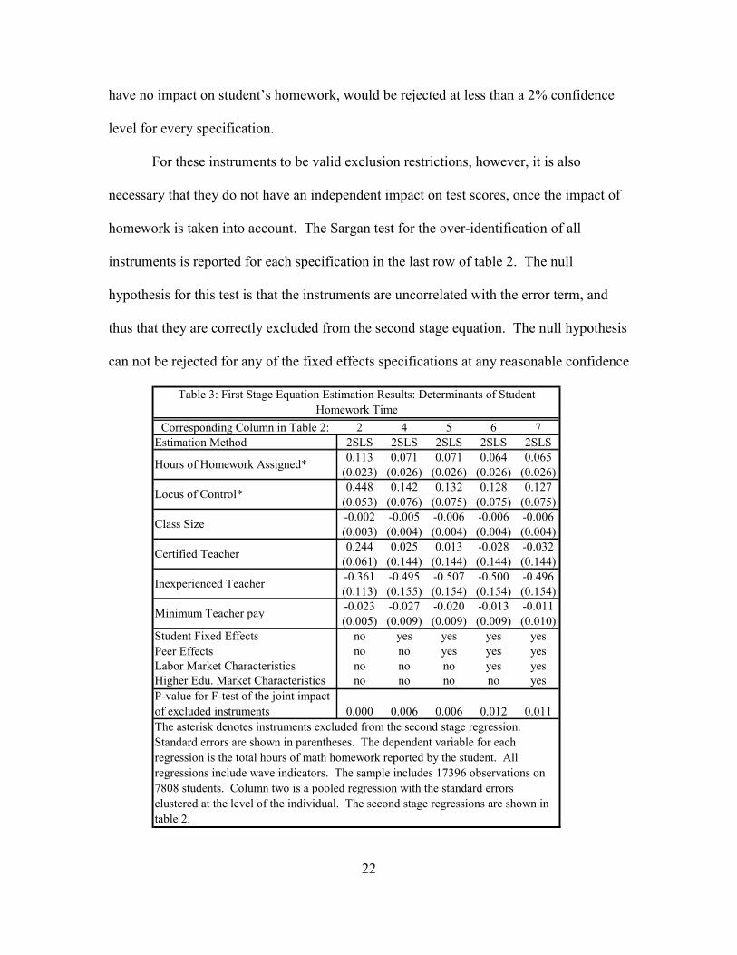
22

have no impact on student’s homework, would be rejected at less than a 2% confidence

level for every specification.

For these instruments to be valid exclusion restrictions, however, it is also

necessary that they do not have an independent impact on test scores, once the impact of

homework is taken into account. The Sargan test for the over-identification of all

instruments is reported for each specification in the last row of table 2. The null

hypothesis for this test is that the instruments are uncorrelated with the error term, and

thus that they are correctly excluded from the second stage equation. The null hypothesis

can not be rejected for any of the fixed effects specifications at any reasonable confidence

Corresponding Column in Table 2: 2 4 5 6 7

Estimation Method 2SLS 2SLS 2SLS 2SLS 2SLS

0.113 0.071 0.071 0.064 0.065

(0.023) (0.026) (0.026) (0.026) (0.026)

0.448 0.142 0.132 0.128 0.127

(0.053) (0.076) (0.075) (0.075) (0.075)

-0.002 -0.005 -0.006 -0.006 -0.006

(0.003) (0.004) (0.004) (0.004) (0.004)

0.244 0.025 0.013 -0.028 -0.032

(0.061) (0.144) (0.144) (0.144) (0.144)

-0.361 -0.495 -0.507 -0.500 -0.496

(0.113) (0.155) (0.154) (0.154) (0.154)

-0.023 -0.027 -0.020 -0.013 -0.011

(0.005) (0.009) (0.009) (0.009) (0.010)

Student Fixed Effects no yes yes yes yes

Peer Effects no no yes yes yes

Labor Market Characteristics no no no yes yes

Higher Edu. Market Characteristics no no no no yes

Inexperienced Teacher

Minimum Teacher pay

Certified Teacher

The asterisk denotes instruments excluded from the second stage regression.

Standard errors are shown in parentheses. The dependent variable for each

regression is the total hours of math homework reported by the student. All

regressions include wave indicators. The sample includes 17396 observations on

7808 students. Column two is a pooled regression with the standard errors

clustered at the level of the individual. The second stage regressions are shown in

table 2.

P-value for F-test of the joint impact

of excluded instruments 0.000

Hours of Homework Assigned*

Class Size

Locus of Control*

Table 3: First Stage Equation Estimation Results: Determinants of Student

Homework Time

0.006 0.006 0.012 0.011

23

level. This test indicates that both the student’s locus of control and the amount of

homework assigned are valid instruments in a fixed effects specification.

Despite this evidence, it is possible that the amount of assigned homework, or the

locus of control, is correlated with past achievement. To test this, I estimate the impact

of a lagged test score on the amount of homework students were assigned, including

some current teacher-related covariates on the right hand side. The results are shown in

table 4. The estimates in the first column show that lagged test scores are strong

0.359 0.139

(0.021) (0.118)

0.180 -0.035

(0.009) (0.037)

-0.001

(0.029)

Locus of

Control

Indpendent

Variable

Lagged Test

Score

Standard errors are shown in parentheses. Each regression includes a

wave indicator, and the specifications in row 2 include teacher pay,

teacher experience and teacher certification variables.

Table 4: Testing Instrument Validity

Lagged Test

Score

Assigned HW

With student

Fixed Effects

Assigned HW

Locus of Control

Dependent

Variable

Without Student

Fixed Effects

predictors of each instrument when student fixed effects are not included. When the

specification includes student fixed effects, however, the coefficient associated with the

lagged test scores can not be distinguished from zero. This indicates that past academic

achievement is not correlated with the instruments when fixed effects are included.

It is also possible that both of the instruments are correlated with the same

unobserved student or school characteristics, and contain the same bias. If this were the

case the Sargan test may still indicate that they are exogenous when they are not. In the

last row and last column of table 4 the locus of control is regressed on the amount of

assigned homework in specification with student fixed effects and period intercepts. In

this specification the student’s locus of control has no effect on the amount of homework

24

that the student is assigned. These variables, therefore, likely do not capture any

common unobserved variables, and do provide exogenous variation in homework time.

Diminishing Returns To Homework Time

So far the econometric model estimated has restricted the impact of homework to

a linear effect, not allowing the possibility of diminishing returns to studying. This

restriction is easily relaxed by estimating a second order polynomial in homework, which

is done in table 5.

1 2 3

Dependent Variable Hours of Math

HW

Hours of Math

HW Squared

Math Test

Score

0.294

(0.059)

-0.013

(0.004)

0.093 0.770

(0.051) (1.080)

-0.003 -0.006

(0.004) (0.084)

0.133 -0.686

(0.075) (1.581)

0.181 4.246

(0.069) (1.457)

-0.006 -0.179 -0.002

(0.004) (0.085) (0.001)

-0.034 -1.803 -0.023

(0.144) (3.025) (0.023)

-0.503 -10.481 -0.007

(0.154) (3.232) (0.033)

-0.011 -0.268 0.001

(0.010) (0.203) (0.002)

Marginal Effect of HW 0.194

Evaluated at the mean (0.043)

Standard errors are in parentheses. The first two columns are the first stage equations;

the third column is the second stage equation. Each regression includes student fixed

effects, peer effects, labor market and higher education market characteristics, and wave

indicators.

Hours of HW Assigned

Locus of Control Squared

Hours of Math Homework

Teacher Certified in Subject

Inexperienced Teacher

Minimum Teacher pay

Hours of Homework Assigned

Squared

Locus of Control

Hours of Math Homework Squared

Table 5: Decreasing Returns to Hours of Homework

Class Size

25

The first two columns show the first stage equations predicting student homework time

and student homework time squared. The instruments excluded from the second stage

equation were the amount of assigned homework, the locus of control, and each of these

instruments squared. For students currently not spending any time doing mathematics

homework, the return on completing one hour of homework a week would be about a 10

percentile point improvement in mathematics test scores. This return decreases as

students spend more time studying. The marginal effect of studying an additional hour if

the student is currently studying the average amount (about 3.7 hours) is a 7.5 percentile

point increase in test scores. These results also indicate that mathematics homework

ceases to improve test scores if a student does more than about 11 hours per week. By

this standard, the majority of students could increase their test scores if they spent more

time on their mathematics homework.

Impact of Homework Time by Achievement Level and School Quality

The econometric model used thus far also restricts the impact of homework to be

the same for all students regardless of their achievement level or school setting. In this

section, I will try to relax this restriction by estimating the specification from table 5

separately for high achieving and low achieving students, as well as high and low

performing schools. First, students are separated into two groups of equal size based on

their mathematics achievement test scores in the 8th grade. The first column of table 6

shows the results. Each specification includes a squared term,15 and thus marginal effects

are reported, evaluated at the mean reported homework time for the entire sample.

15 The effect is similar if the squared term is not included. The second order polynomial is used in this section because this specification results in more precise estimates.

26

0.344 0.485

(0.089) (0.246)

-0.015 -0.027

(0.004) (0.017)

0.231 0.279

(0.067) (0.157)

0.224 0.234

(0.111) (0.063)

-0.010 -0.010

(0.009) (0.004)

0.150 0.161

(0.053) (0.041)

The impact is measured by the coefficients associated with an hour

of homework per week in an instrumental variables regression with

student fixed effects, where the dependent variable is the

Mathematics achievement test score. Student achievement is

measured by the student's 8th grade mathematics test score. School

quality is measured by the average mathematics test score of all other

observed students in the same school.

Table 6: Impact of Homework Time by Student Achievement and

School Quality

Marginal Effect

Hours of Math Homework

Math HW Squared

Marginal Effect

Bottom

Half

Hours of Math Homework

Math HW Squared

Student

Achievement

School

Quality

Top Half

Group

The students in the lower achieving group experience much higher returns to

studying than those in the high achievement group. The impact of an hour of homework

for the low-achievement group is large enough to improve a student’s mathematics

achievement by 8.5 percentile points. An additional hour of homework by a high

achieving student, however, only improves their achievement by 5.5 percentile points.

This indicates that students who fall behind do have some ability to catch up to their

peers simply by doing the same amount of homework. For example, consider a student

in the low achievement group, who is currently spending one hour on homework each

week. By studying 2.5 hours more per week, this student could move from the 25th

percentile to the 50th percentile in a single year. A student in the high achievement

group, who is currently studying one hour a week, would have to study 4.4 additional

27

hours each week to make a similar move from the 50th to the 75th percentile. This

evidence does not support the common assumption that more able students receive a

higher return to homework time because their time is more productive (Neilson, 2005;

Eren and Henderson, 2007).

Second, students were split into groups of equal size based on the test score

performance of their peers, as a general measure of school quality. Students in the lower

performing schools experienced a return to homework time that was twice as strong as

those in high performing schools. A student in a low performing school, who currently

studies one hour each week that wanted to move from the 50th percentile to the 75th

percentile, would have to study 1.8 additional hours per week, whereas a student in a high

performing school would have to study four additional hours to improve the same

amount. This may indicate that at low performing schools homework is a stronger

determinant of success. Bishop (2007) reports that less material is presented in class time

in low performing schools, which may partially explain why studying at home would be

more beneficial for these students. Overall, this investigation yields the finding that

students’ achievement in mathematics can be dramatically improved by effort, even if the

student finds herself at the bottom end of the achievement distribution in a low

performing school.

Impact of Assigned Homework on Academic Achievement

While students are able to adjust the amount of time they spend on homework

directly, the more realistic policy instrument is the amount of homework that teachers

assign. Teachers’ assignments, even if only completed a fraction of the time, have a

28

strong influence on the amount of homework students complete. For comparison, the

regression below shows the impact of a series of policy instruments, including the

amount of mathematics homework assigned by teachers per week (hit), on a mathematics

test score (TSit):16

(12) 0.009 0.001 0.020 0.015 0.002

(0.003) (0.0006) (0.021) (0.024) (0.001)

it it it it it it i itTS h s c x p µ ε= − − − + + +

Where sit is the school class size, cit indicates that the teacher is certified in mathematics,

xit is the fraction of the students’ observed teachers that have less than three years of

teaching experience, pit is the minimum teacher pay in the students’ school, iµ is a

student specific intercept or fixed effect, and itε is the error term.17 The effects of

teacher certification and teacher experience are not precisely estimated; neither effect is

statistically different from zero at any reasonable confidence level. These two policies

are excluded from the following analysis.

To compare the size of these effects, it is useful to do a comparison of cost of

implementing each policy, and the resulting academic achievement gains. Table 7 shows

the impact of a $10,000 investment in three possible policies. To approximate the social

Policy Impact: SD Impact: Percentile Points

Increasing Assigned Homework 0.058 2.32

Increasing Teachers' Wages 0.020 0.80

Decreasing Class Size 0.005 0.21

Results are calculated using the coefficients reported in equation 12, an average class size of 25,

average yearly teachers' wage of $47,602, an hourly wage of $29.75 for teachers, and a minimum

wage of $5.68 for students. See appendix C for calculations.

Table 7: Impact of a $10,000 per classroom investment:

16 This regression is on a smaller sample of 9776 observations on 4990 students. This is the sample of students who have multiple responses by a mathematics instructor. The larger sample consists of students who study math but may or may not have had a mathematics instructor interviewed. 17 For the full results from the regression shown in equation 12, see appendix B.

29

cost of assigning more homework, I assume that teachers are paid almost $30 an hour for

their time. The time of the students who do additional homework because of the policy is

valued at the 1990 minimum wage, converted to 2005 dollars. The cost of decreasing

class size is limited here to the cost of hiring additional teachers. The cost of building

new classrooms and the impact of decreasing teacher quality are not considered here.

The first column shows the impact in on mathematics achievement in standard

deviations, the second shows the impact in percentile point improvements. Assigning

additional homework is estimated to have almost three times the impact of increasing

teachers’ wages for a given monetary investment. Similarly, assigning additional

homework has over 11 times the impact per dollar of decreasing class size.

Finally, it is worth exploring whether this policy will have a differential impact

based on school quality and prior student achievement. Table 8 shows the impact of

assigning additional mathematics homework for the top and bottom halves of the

achievement and school quality distributions. The impact is estimated with similar

Prior Achievement School Quality

0.003 0.002

(0.004) (0.004)

0.015 0.013

(0.005) (0.005)

Standard errors are shown in parentheses. For each result, assigned homework is used to

predict mathematics achievement in a student fixed effect regression specification. Teacher

experience, certification, salary, class size, peer effects, and wave indicators were also

included in each specification. Prior Achievement is measured using the students' 8th grade

mathematics achievement scores. School quality is measured using the average test score of

other observed students in the same school.

Top Half

Bottom Half

Table 8: Impact of Assigned Homework on Mathematics Achievement by Achievement and

School Quality

precision for each subgroup, but the impact is not statistically different from zero for

those with high 8th grade mathematics achievement or for those with high performing

peers. The effect, however, is quite strong for low-performing students and those in low-

30

performing schools. Assigning an additional hour of homework per week to a student

who is below the 50th percentile in 8th grade math achievement is estimated to improve

their achievement by 3/5th of a percentile point. Comparing this effect to the impacts in

table 7, a $10,000 investment put into increasing homework for a classroom of students

in this low-performing group would increase each student’s achievement by .096

standard deviations, or 3.87 percentile points. This effect is larger than the impacts of

similar investments in homework, teachers’ wages or class sizes shown in table 7.

VII. Conclusions

The main findings of this paper are clear: students’ achievement is not determined

primarily by school characteristics or teacher training, but seems to be much more

dependent on the choices that students make. In the case of students who are performing

significantly less well than their peers, or who find themselves in low performing

schools, the evidence indicates that opportunities to improve their achievement are

available. The return to studying is much higher for these students, and it may be

possible for them to catch up to their peers, or make up for a poor school, with small

increases in the amount of time they invest in homework.

As a tool of policy, increasing the amount of homework that students complete

shows some promise. Assigning additional homework is estimated to have a much larger

impact per dollar invested than either increasing teachers’ wages or decreasing class

sizes. Additionally, because much of the benefit of assigning additional homework goes

to low-achieving students and students in low-performing schools, this policy could be

31

useful for lowering the achievement gap between high achieving and low achieving

students.

References

Aksoy, Tevfik, and Charles R. Link. (2000) “A Panel Analysis of Student Mathematics Achievement in the US in the 1990s: does increasing the amount of time in learning activities affect math achievement?” Economics of Education Review. 19: 261-277. Altonji, Joseph G. and Thomas A. Dunn. (1996). “Using Siblings to Estimate the Effect of School Quality on Wages,” The Review of Economics and Statistics, 78(4)(November): 665-671 American Federation of Teachers (2007) “Survey and Analysis of Teacher Salary Trends 2005” Washington D.C. Betts, J. (1996). “The Role of Homework in Improving School Quality.” Discussion Paper 96-16. Department of Economics, UCSD. Bishop, John. (1991) “Achievement, Test Scores, and Relative Wages.” in Workers and

Their Wages: Changing Patterns in the United States. Marvin Kosters ed. Washington D.C.: AEI Press. Bishop, John. (2007) “Drinking from the Fountain of Knowledge: Student Incentive to Study and Learn – Externalities, Information Problems, and Peer Preasure.” In The Handbook of the Economics of Education. Eric Hanushek and Finis Welch, eds. Blau, David. (1999) “The Effect of Income on Child Development.” The Review of Economics and Statistics. 81(2):261-276. Cooper, Harris, Jorgianne Robinson and Erika Patall. (2006) “Does Homework Improve Academic Achievement? A Synthesis of Research.” Review of Educational Research. 76(1)(spring): 1-62. Cunha, Flavio, James Heckman, Lance Lochner, and Dimitryi Masterov. (2007) “Interpreting the Evidence on Life Cycle Skill Formation.” The Handbook of the Economics of Education. E. Hanusheck and F. Welch, eds. Dahl, Gordon B. and Lance Lochner. (2005). “The Impact of Family Income on Child Achievement,” Working Paper 11279. Cambridge, MA: National Bureau of Economic Research. Eren, Ozkan, and Daniel J. Henderson. (2007) “The Impact of Homework on Student Achievement.” Working Paper.

32

Hall, A.R., Rudebusch, G.D. and Wilcox, D.W. (1996). “Judging Instrument Relevance in Instrumental Variables Estimation.” International Economic Review, 37(2): 283-298. Hanushek, Eric A. (1998) “The Evidence on Class Size,” University of Rochester Occasional Paper number 98-1. Hanusheck, Eric A., John F. Kain, and Steven G. Rivkin. (1998) “Teachers, Schools, and Academic Achievement.” Presented at the annual meetings of the Econometric Society, Chicago. Hanushek, Eric A., John F. Kain, Jacob M. Markman, Steven G. Rivkin. (2003) “Does Peer Ability Affect Student Achievement?” Journal of Applied Econometrics 18(5): 527-544. Hanushek, Eric A. (2003). “The Failure of Input-Based Schooling Policies,” The Economic Journal, 113(February): F64-F98. Hanushek, Eric A., and Steven G. Rivkin. (2006) “School Quality and the Black-White Achievement Gap,” National Bureau of Economic Research Working Paper No. 12651. Hanushek, Eric A., and Steven G. Rivkin (2007) “Teacher Quality.” In The Handbook of the Economics of Education. Hanushek and Rivkin eds. Harmon, Maryellen, Teresa A. Smith, Michael O. Martin, Dana L. Kelly, Albert E. Beaton, Ina V.S. Mullis, Eugenio J. Gonzalez, and Graham Orpwood. (1997) Performance Assessment in IEA's Third InternationalMathematics and Science Study, The International Study Center at Boston College, September. Hill, Lester, Jr. (1991). “Effort and Reward in College: A Replication of Some Puzzling Findings.” In Replication Research in the Social Sciences, James W. Neuliep, ed. Newbury Park, CA: Sage. 139-156. Hoxby, C.M. (1999) “The Productivity of Schools and Other Local Public Good Producers,” Journal of Public Economics, 74: 1-30.

Manski, Charles F. (1993) “Identification of Endogenous Social Effects: The Reflection Problem.” The Review of Economic Studies 60(3): 531-542

McMullen, Steven (2007) “The Labor Market Determinants of Student Homework Time in High School.” Working Paper. Neilson, William. (2005) “Homework and Performance for Time-Constrained Students.” Economics Bulletin, 9(1): 1-6. Parker, Angie. (1999) “A Study of Variables that Predict Dropout from Distance Education.” International Journal of Educational Technology 1(2).

33

Rau, William and Ann Durand (2000). “The Academic Ethic and College Grades: Does Hard Work Help Students to ‘Make the Grade’?” Sociology of Education 73: 19-38. Sacerdote, Bruce. (2001) “Peer Effects with Random Assignment: Results for Dartmouth Roommates,” Quarterly Journal of Economics 116(2): 681-704. Shuman, Howard, Edward Walsh, Camille Olson, and Barbara Etheridge (1985). “Effort and Reward: The Assumption that College Grades are Affected by the Quantity of Study.” Social Forces 63:945-66. Steptoe, Andrew and Jane Wardle. (2001) “Locus of Control and Health Behavior Revisited: A Multivariate Analysis of Young Adults from 18 Countries.” British Journal of Psychology. 92:659-672. Stinebrickner, Todd, and Ralph Stinebrickner (2007). “The Causal Effect of Studying on Academic Performance.” National Bureau of Economic Research Working Paper number 13341. Todd, Petra E. and Kenneth Wolpin (2003) “On the Specification and Estimation of the Production Function for Cognitive Achievement,” The Economic Journal 113(485) F3-F33. Todd, Petra E. and Kenneth I. Wolpin. (2004) “The Production of Cognitive Achievement in Children: Home, School, and Racial Test Score Gaps.” Penn Institute for Economic Research Working Paper 04-019. Wang, Alvin Y., and Michael H. Newlin (2000) “Characteristics of Students who Enroll and Succeed in Psychology Web-Based Classes.” Journal of Educational Psychology. 92(1): 137-143. Zimmerman, David J. (2003) “Peer Effects in Academic Outcomes: Evidence from a Natural Experiment,” The Review of Economics and Statistics 85(1): 9-23.

34

Appendix A: Variable Definitions Mathematics Test Scores: The cognitive tests were given to students with each survey, and varied according to students’ past performance. For this reason, raw scores are not used, but instead the scores are normalized across waves, and I divided the variables by 10 within each year so that the standard deviation is approximately equal to 1. The tests were created to allow comparison across grades, and to accurately measure student achievement even if students do not complete the entire exam. Hours of Mathematics Homework: This variable measures the number of hours that the student spends per week on mathematics homework. The NELS data records the hours of homework completed in a series of categories. Each student is assigned the mean value for their category. Class Size: This is defined as the average size of the observed classes taken by the student in each wave. Teacher Has Certification in Field: This variable equals 1 if all of the teachers surveyed for this student have the certification to teach the class that the student is taking. It equals 0.5 if one teacher is certified and the other is not, and it equals 0 if all of the teachers surveyed are not certified. Inexperienced Teacher: This indicator variable is equal to one if the teacher interviewed has three or less years of experience. The source variables did not allow for separate indicators for one, two, and three years of experience. Minimum Teachers’ Wage: This variable comes from the school counselors’ survey, and records the minimum annual wage for a teacher in the school that the student is attending. This variable is adjusted so that it is measured in units of 1000 1995 dollars.

Assigned Homework: This is a continuous variable recording the average hours per week that the students’ interviewed teachers assigned. The source variables were all continuous, though the base year was a weekly variable and the second and third waves asked for daily amounts. I multiplied the daily homework amounts by 5 to get the weekly amount. Locus of Control: This is a composite of three questions, which measures the degree to which the student has an “internal” locus of control. Students with an internal locus believe that their actions and choices can shape their future, where students with an external locus believe external events will be the primary determinants of what their future is like. A higher number indicates that the students’ locus is more internal. The questions ask the student to agree or disagree (five point scale) with the following statements: “In my life, good luck is more important than hard work for success.” “Every time I try to get ahead, something or somebody stops me.” “My plans hardly ever work out, so planning only makes me unhappy.”

35

Unemployment Rate: The unemployment rate for the students’ state of residence, for a given year. Minimum Wage: The highest legally binding unemployment rate for the student’s state of residence, either the statewide or federal minimum. Industry Mix: An industry-education index. This variable takes the nation-wide average education level for employees in a given industry based on the 1990 IPUMS CPS march supplement. The index is a sum of this statistic for each industry in the state, weighted by the number of people in the state that are employed in that industry. Average Public Four-Year Tuition: The average tuition cost per year for in state residents at four year public institutions. In units of 1000 1995 dollars. Financial Aid Per Student: The amount of state-provided financial aid for college students, per student. In units of 1000 1995 dollars. Appropriations Per Student: The amount of money allocated by the state for higher education, per student. In units of 1000 1995 dollars.

36

Appendix B: Full Regression Output

1 2 3

0.243

(0.086)

0.065 0.009

(0.026) (0.003)

0.127

(0.075)

-0.006 0.000 -0.001

(0.004) (0.001) (0.001)

-0.032 -0.001 -0.020

(0.144) (0.037) (0.021)

-0.496 0.106 -0.015

(0.154) (0.058) (0.023)

-0.011 0.004 0.002

(0.010) (0.003) (0.001)

0.001 0.001 0.001

(0.001) (0.000) (0.000)

0.117 -0.029 -0.002

(0.018) (0.011) (0.002)

-0.996 0.262

(0.197) (0.100)

0.063 -0.017

(0.014) (0.007)

0.285 -0.104

(0.234) (0.065)

0.229 -0.089

(0.525) (0.136)

0.091 -0.022

(0.210) (0.210)

-0.499 0.206

(0.508) (0.137)

-0.082 0.016

(0.078) (0.021)

3.599 -0.351 0.521

(0.114) (0.316) (0.011)

3.325 0.165 0.972

(0.299) (0.300) (0.023)

3.997

(0.085)

No. of Observations 17610 17610 9776

No. of Students 7902 7902 4990

Hours of

Homework

Mathematics

Test Scores

Mathematics

Test Scores

Table B1: Full Regression Output for the Main Results

Wave 2 Indicator

Wave 3 Indicator

Constant

Dependent Variable:

Average Peers' Test Score

State Unemployment Rate

Industry Mix

State Public four year

tuition

State Financial Aid Per

Student

State Higher Ed.

Appropriations Per

Average Peers' HW Time

State Unemployment Rate

Squared

Minimum Wage

Standard errors are reported in parentheses. The first column shows the full

results for the first stage equation shown in table 3 column 7. The second column

shows the second stage results from table 2 column 7, and the last column shows

the results displayed in equation 12. All equations include student fixed effects.

The homework used in column two is the value of homework time predicted by

the specification in column one.

Teachers are Certified in

Subject Matter

Inexperienced Teachers

Minimum Teacher Wage

Locus of Control

Hours of Mathematics

Homework

Hours of Assigned

Homework

Class Size

37

Appendix C: Policy Comparison Results shown in table 7. Assigning Additional Homework:

Average Annual Teacher Salary for 2005: $47,602 (American Federation of Teachers 2007) Hourly wage: $47,602 a year / 40 weeks per year / 40 hours per week = $29.75 per hour. I assume that 1 hour of assigned homework takes the teacher 1 hour to prepare and record. So a one hour increase in homework per week would cost the teacher $29.75 per week for 40 weeks, totaling $1190. The students are assumed to complete an additional .065 hours of homework per hour assigned (see table 3). The students’ time is valued at the 1990 federal minimum wage, which in 2005 dollars is $5.68 per hour. Assuming the class includes 25 students, the student cost of an additional hour of assigned homework for one week is $9.23. Over 40 weeks, the total cost to students is $369. Thus the total social cost of assigning one additional hour of homework per year is $1559. A $10,000 investment in additional assigned homework could “buy” 6.42 hours of homework per year. This homework investment, multiplied by the homework coefficient from equation 12 is 6.42*.009 which is a 0.058 standard deviation increase. This would result in a class wide increase in math achievement of 2.32 percentile points. Increasing Class Size

The average class size observed in the NELS data is 25 students. The cost of decreasing a class by one student is therefore roughly 1/25th of the cost of a teacher’s annual salary. So $47,602/25 = $1904 is the relevant cost. This understates the cost if there are space constraints, and the schools need to find additional classroom space or build new schools. A $10,000 investment in class size reduction per classroom would thus be enough to reduce classes by 5.25 students. This reduction, according to the impact estimated in equation 12, would increase students’ mathematics achievement by 0.00525 standard deviations. This corresponds to a change of .21 percentile points. This impact is overestimated, however, if lower quality teachers are hired in order to reduce class size. Increasing Teachers’ Wages

The only teachers’ pay measure available in the NELS data across all three waves is the minimum full time teacher’s wage. Since most teachers get paid according to a district-wide scale that depends on education and experience, the minimum wage is probably a

38

good measure of the impact of wages, since it will not be confounded with the impact of teachers’ education or years of experience. The impact associated with increasing a teachers’ wage by $10,000 is ten times the impact shown in equation 12, which amounts to 0.02 standard deviations. This effect would increase the mathematics achievement by 0.8 percentile points.