The impact of banks’ capital adequacy regulation on the economic system: an agent‐based approach 

Andrea Teglio Marco Raberto Silvano Cincotti 

2011 / 01 

The impact of banks’ capital adequacy regulation on the economic system: an agent-based

Andrea Teglio Universitat Jaume I

Department of Economics teglio@uji.es

Marco Raberto University of Genova

marco.raberto@unige.it

Silvano Cincotti University of Genova

silvano.cincotti@unige.it

2011 / 01

Abstract

Since the start of the financial crisis in 2007, the debate on the proper level leverage of financial institutions has been flourishing. The paper addresses such crucial issue within the Eurace artificial economy, by considering the effects that different choices of capital adequacy ratios for banks have on main economic indicators. The study also gives us the opportunity to examine the outcomes of the Eurace model so to discuss the nature of endogenous money, giving a contribution to a debate that has grown stronger over the last two decades. A set of 40 years long simulations have been performed and examined in the short (first 5 years), medium (the following 15 years) and long (the last 20 years) run. Results point out a non-trivial dependence of real economic variables such as the Gross Domestic Product (GDP), the unemployment rate and the aggregate capital stock on banks’ capital adequacy ratios; this dependence is in place due to the credit channel and varies significantly according to the chosen evaluation horizon. In general, while boosting the economy in the short run, regulations allowing for a high leverage of the banking system tend to be depressing in the medium and long run. Results also point out that the stock of money is driven by the demand for loans, therefore supporting the theory of endogenous nature of credit money.

Keywords: Agent-based models, banking regulation JEL Classification: G2

The impact of banks’ capital adequacy regulationon the economic system: an agent-based

approach

Andrea Teglio ∗ Marco Raberto † Silvano Cincotti †

April 26, 2011

Abstract

Since the start of the financial crisis in 2007, the debate on the proper levelleverage of financial institutions has been flourishing. The paper addresses suchcrucial issue within the Eurace artificial economy, by considering the effects thatdifferent choices of capital adequacy ratios for banks have on main economic in-dicators. The study also gives us the opportunity to examine the outcomes of theEurace model so to discuss the nature of endogenous money, giving a contributionto a debate that has grown stronger over the last two decades. A set of 40 yearslong simulations have been performed and examined in the short (first 5 years),medium (the following 15 years) and long (the last 20 years) run. Results point outa non-trivial dependence of real economic variables such as the Gross DomesticProduct (GDP), the unemployment rate and the aggregate capital stock on banks’capital adequacy ratios; this dependence is in place due to the credit channel andvaries significantly according to the chosen evaluation horizon. In general, whileboosting the economy in the short run, regulations allowing for a high leverage ofthe banking system tend to be depressing in the medium and long run. Resultsalso point out that the stock of money is driven by the demand for loans, thereforesupporting the theory of endogenous nature of credit money.

IntroductionThe agent-based modelling approach applied to economics allows to take into accountthe complex pattern of interactions among different economic agents in a realisticand complete way. The Eurace simulator is an agent-based model of the macroecon-omy characterized by different kinds of agents, namely, households, firms, commer-cial banks, a Government and a Central Bank, and by different decentralized markets,characterized by pairwise exchange interactions, such as a labor market, a goods mar-ket, and a credit market; a financial market is also present, where firm equity shares

∗Departament d’Economia, Universitat Jaume I, Castellon de la Plana 12071, Castellon, Spain†University of Genova, Via Opera Pia 11a, 16145, Genova Italy

1

and government bonds are exchanged in a centralized way through a clearing house[14, 24].

This paper investigates the impact of bank lending regulation on macroeconomicactivity by considering a set of economic variables as indicators. The regulatory pa-rameter considered is the leverage ratio of commercial banks, i.e. the ratio between thevalue of the loan portfolio held by banks, weighted with a measure of the loan riski-ness, and banks net worth or equity, along the lines of capital adequacy ratios set bythe Basel II agreement [1].

The debate on implications and consequences of capital adequacy requirements forbanks has been growing in the last three decades [10, 11] and has drawn particularattention after the financial crisis of 2007-2009 [19, 7]. The discussion focuses onthe beneficial effects of equity requirements compared to the disadvantages in terms ofeconomic costs and credit market effectiveness. Some of the main controversial aspectsabout the implications of higher equity requirements are clearly resumed in [6]. Themain benefit of increased equity capital requirements is claimed to be the weakeningof systemic risk, while potential drawbacks are, among others, the reduction of returnon equity (ROE) for banks, the restriction of lending, and the increase of funding costsfor banks. This paper focuses on the macroeconomic implications of capital adequacyregulation, studying its effect on banks’ lending activity and therefore on the maineconomic indicators such as GDP, unemployment and inflation. In particular, threedifferent time horizons are considered (short, medium and long run) in order to analyzethe macroeconomic outcomes of the Eurace artificial economy so to take into accountalso the long-term effects.

The long-term macroeconomic impact of capital requirements has been intensivelyexamined after the last financial crisis, see [5, 3, 4] and [8] for some complete and rep-resentative studies by central banks or by international institutions performing policyanalysis and financial advising, like the BIS1 or the IIF2. An analysis of these reports,along with a critical assessment of the used models, is beyond the scope of this paper.Let us simply summarize the main common results. Firstly, higher capital requirementsreduce the probability of banking crises. Secondly, it emerges that an increase in thecapital ratio causes a decline in the level of output; the magnitude of the effect dependson the specific model. Thirdly, a higher capital ratio tends to dampen output volatility,especially if counter-cyclical capital buffers schemes are adopted. These main resultshave been obtained using a variety of models (see [3] for a list), mainly DynamicStochastic General Equilibrium (DSGE) models or semi-structural models. DSGE canbe considered as the standard type of model currently used in macroeconomics, eventhough they have been widely criticized both for their difficulties in explaining someeconomic phenomena (see for instance [12, 20]) and for the fact that the assumed equiv-alence between the micro and the macro behavior in DSGE models does not allow totake properly into account interaction and coordination among economic agents [13].

The aim of this study is to present an alternative approach based on a fully en-dogenous agent-based model whose dynamics does not depend on external stochasticprocesses but mainly on the interaction of economic agents populating the artificial

1The Bank for International Settlements; http://www.bis.org2The Institute of International Finance, Inc.; http://www.iif.com/

2

economy. See [25] for a comprehensive survey on agent-based computational eco-nomics and [2] for an overview of the Eurace model.

In concrete terms, a set of computational experiments have been carried out withthe objective to study the performance of the economic system according to differentvalues of the capital ratio requirement. The outcomes of this what-if analysis show howthe main macroeconomic variables characterizing the Eurace economy, i.e. both realvariables (such as GDP, unemployment and capital stock), and nominal variables (suchas wage and price levels) are affected by the aggregate amount of loans provided bybanks, which in turn depends on banks net worth or equity and on the allowed leverageratio.

The interpretation of results can be possibly done in accordance with the lines of theendogenous credit-money approach of the post-Keynesian tradition [17, 9, 21]. Con-trary to the neoclassical synthesis, where money is an exogenous variable controlled bythe central bank through its provision of required reserves, to which a deposit multiplieris applied to determine the quantity of privately-supplied bank deposits, the essenceof endogenous money theory is that in modern economies money is an intrinsicallyworthless token of value whose stock is determined by the demand of bank credit bythe production or commercial sectors and can therefore expand and contract regard-less of government policy. Money is then essentially credit-money originated by loanswhich are created from nothing as long as the borrower is credit-worthy and some in-stitutional constraints, such as the Basel II capital adequacy ratios, are not violated. Asthe demand for loans by the private sector increases, banks normally make more loansand create more banking deposits, without worrying about the quantity of reserves onhand, and the central bank usually accommodates the demand of reserves at the shortterm interest rate, which is the only variable that the monetary authorities can control.

The modeling architecture of the Eurace economy, which has been conceived inorder to closely mimic the functioning of a modern credit-driven economy, stronglyconfirms the endogenous theory view. Based on this conceptual framework, we inves-tigate the relationship between endogenous credit money and macroeconomic activity,by examining computational experiments where the institutional (e.g. Basel II) con-straints on bank leverage are exogenously set.

The paper is organized as follows. In section 1 an overall description of the creditmarket model is given, both considering the firms and the banks sides. Section 2presents the computational results of our study and a related discussion. Conclusionsare drawn in section 3.

1 The credit market modelIn the following, we outline the main features of the Eurace credit market model bydescribing how the demand of credit by firms arises to finance their production and liq-uidity needs, how the supply of credit by banks is conditioned by their capital adequacyratio and how borrowers (firms) and lenders (banks) match their respective demand andsupply schedules in the market.

3

1.1 Firms’ sideTwo types of firms are considered in the Eurace model: capital goods producers andconsumption goods producers. Capital goods producers employ labor to produce on jobcapital goods that will be used as production factor together with labor by consumptiongoods producers. Given job production and only labor as production factors, capitalgoods producers, contrary to consumption goods producers, have not inventories aswell as financing needs. In the following we will describe in more detail consumptiongoods producers, henceforth generally identified as firms.

Once a month, every firm computes its total liquidity needs, given by the liquid-ity necessary to meet its financial payments and by the expected cost of the plannedproduction schedule. In particular, firm f at month t is subject to the following finan-cial payments: the interest payments on its debt, henceforth R f

t , the debt installment,henceforth I f

t , taxes T ft and dividends payments D f

t . The total liquidity needs L ft of firm

f are therefore given by L ft = C f

t +R ft + I f

t +T ft +D f

t , where C ft are the the expected

costs of the planned production schedule.Firms plan the monthly production schedule by considering the stock of inventories

kept by the different malls selling their products, and by estimating the demand usinga linear regression based on previous demands. Production is carried out according toa Cobb-Douglas type function, with two factors of production, i.e. labor and capital; adesired capital to labor ratio is calculated considering the marginal rate of substitutionof the two factors, which depends on the given money wage and the cost of capital.Given the planned monthly production schedule and the desired capital to labor ratio,the desired capital endowment and the labor demand are determined by inverting theCobb-Douglas production function. Demand for investments then depends on the dif-ference between the desired and the actual capital endowment (see [15, 16] for details).

According to the pecking-order theory [22], any firm f meets its liquidity needsfirst by using its internal liquid resources P f

t , i.e., the cash account deposited at a givenbank; then, if P f

t < L ft , the firm asks for a loan of amount L f

t −P ft to the banking system

so to be able to cover entirely its foreseen payments. Credit linkages between firm fand bank b are defined by a connectivity matrix which is randomly created whenever afirm enters the credit market in search for funding. In order to take search costs as wellas incomplete information into account, each firm links with a maximum of n banks ofthe same region, which are chosen in a random way.

Firms have to reveal to the linked banks information about their current equity anddebt levels, along with the amount of the loan requested λ f

t . Using this information,according to the decision rules outline din the next section, each contacted bank bdetermines the amount of money available for lending to firm f (henceforth ℓ f

t , whereℓ f

t ≤ λ ft ), calculates the interest rate ib f

t associated to the loan and communicates it tothe firm. After this first consulting meeting where firm’s credit worthiness has beenassessed by the bank, each firm asks for credit starting with the bank with the lowestinterest rate. On banks’ hand, they receive demands by firms sequentially and dealwith them in a “first come, first served” basis. As explained with more detail in thefollowing section, the firm can be credit rationed. If a firm can not obtain a sufficientamount of credit from the bank that is offering the best interest rate, the firm will ask

4

credit to the bank offering the second best interest rate, until the last connected bank ofthe list is reached. It is worth noting that, although the individual firm asks loans to thebank with the lowest lending rate, the total demand for loans does not depend directlyon the interest rates of loans.

When firm f receives a loan, its cash account P ft is then increased by the amount

of it. If the firm is not able to collect the needed credit amount, i.e., if P ft is still lower

than L ft , the firm has still has the possibility to issue new equity shares and sell them

on the stock market. If the new shares are not sold out, the firm enters a state calledfinancial crisis. When a firm is in financial crisis, we mainly distinguish two cases (see[2] for further details): if the firm’s available internal liquidity is still sufficient to meetits committed financial payments, i.e., taxes, the debt instalment and interests on debt,then these financial payments are executed and the dividend payout and the productionschedule are rearranged to take into account the reduced available liquidity; otherwise,the firm is unable to pay it financial commitments and it goes into bankruptcy.

1.2 Banks’ sideThe primary purpose of banks is to channel funds received from deposits towards loansto firms. When a firm f contacts a bank b to know its credit conditions, the firm has toinform the bank about its equity level E f

t and its total debt D ft , defined as the sum of

the loans that the firm has received from every bank and that it has not yet payed back.Any bank meets the demand for a loan, provided that the risk-reward profile of the loanis considered acceptable by the bank. The reward is given by the interest rate which ischarged and the risk is defined by the likelihood that the loan will default. Given theloan request amount λ f

t by firm f , bank b calculates the probability that the firm willnot be able to repay its debt as:

π ft = 1− e

−(

D ft +λ f

tE f

t

). (1)

The default probability π ft correctly increases with the firm’s leverage and is used as

a risk weight in computing the risk-weighted loan portfolio of banks, henceforth W bt .

According to the computed credit worthiness of the firm, the bank informs it about theinterest rate that would be applied to the requested loan:

ib ft = ict + γb

t ·πf

t , (2)

where ict is the interest rate set by the central bank and γbt ·π

ft is the risk spread depend-

ing on the firm’s credit risk. The parameter γbt sets the spread sensitivity to the credit

worthiness of the firm and is an evolving parameter that basically adjusts in order toreinforce the previous choices that were successful in increasing the bank’s profits. Thecentral bank acts as the “lender of last resort”, providing liquidity to the banking sectorat the interest rate ict . Finally, it is worth noting that banks lending rate does not dependon the expected demand for loans but only on the evaluation of firm’s credit risk.

Banks can then lend money, provided that firms wish to take out new loans and thattheir regulatory capital requirement are fulfilled. It is worth noting that granting new

5

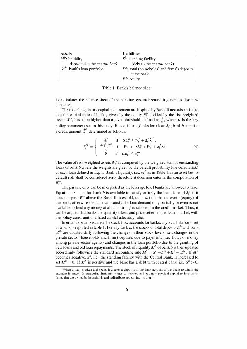
Assets LiabilitiesMb: liquidity Sb: standing facility

deposited at the central bank (debt to the central bank)L b: bank’s loan portfolio Db: total (households’ and firms’) deposits

at the bankEb: equity

Table 1: Bank’s balance sheet

loans inflates the balance sheet of the banking system because it generates also newdeposits3.

The model regulatory capital requirement are inspired by Basel II accords and statethat the capital ratio of banks, given by the equity Eb

t divided by the risk-weightedassets W b

t , has to be higher than a given threshold, defined as 1α , where α is the key

policy parameter used in this study. Hence, if firm f asks for a loan λ ft , bank b supplies

a credit amount ℓb ft determined as follows:

ℓb ft =

λ f

t if αEbt ≥W b

t +π ft λ f

t ,αEb

t −W bt

π ft

if W bt < αEb

t <W bt +π f

t λ ft ,

0 if αEbt ≤W b

t .

(3)

The value of risk-weighted assets W bt is computed by the weighted sum of outstanding

loans of bank b where the weights are given by the default probability (the default risk)of each loan defined in Eq. 1. Bank’s liquidity, i.e., Mb as in Table 1, is an asset but itsdefault risk shall be considered zero, therefore it does non enter in the computation ofW b

t .The parameter α can be interpreted as the leverage level banks are allowed to have.

Equations 3 state that bank b is available to satisfy entirely the loan demand λ ft if it

does not push W bt above the Basel II threshold, set at α time the net worth (equity) of

the bank, otherwise the bank can satisfy the loan demand only partially or even is notavailable to lend any money at all, and firm f is rationed in the credit market. Thus, itcan be argued that banks are quantity takers and price setters in the loans market, withthe policy constraint of a fixed capital adequacy ratio.

In order to better visualize the stock-flow accounts for banks, a typical balance sheetof a bank is reported in table 1. For any bank b, the stocks of total deposits Db and loansL b are updated daily following the changes in their stock levels, i.e., changes in theprivate sector (households and firms) deposits due to payments (i.e. flows of moneyamong private sector agents) and changes in the loan portfolio due to the granting ofnew loans and old loan repayments. The stock of liquidity Mb of bank b is then updatedaccordingly following the standard accounting rule Mb = Sb +Db +Eb −L b. If Mb

becomes negative, Sb, i.e., the standing facility with the Central Bank, is increased toset Mb = 0. If Mb is positive and the bank has a debt with central bank, i.e. Sb > 0,

3When a loan is taken and spent, it creates a deposits in the bank account of the agent to whom thepayment is made. In particular, firms pay wages to workers and pay new physical capital to investmentfirms, that are owned by households and redistribute net earnings to them.

6

Sb is partially or totally repaid for a maximum amount equal to Mb. Finally, at the endof the trading day, both liquidity Mb and equity Eb are updated to take into account inthe same way of any money flows which regards the bank b, i.e., interest revenues andexpenses, taxes and dividends. The bank can choose if to pay or not to pay dividends toshareholders and this choice is crucial for driving the equity dynamics. In particular, ifa bank is subject to credit supply restriction due to a low net worth compared to the risk-weighted assets portfolio, then it stops paying dividends so to raise its equity capitaland increaser the chance to match in the future the unmet credit demand. Finally, loansare extinguished in a predetermined and fixed number of constant installments.

For a more detailed explanation of the stock-flow accounts in the Eurace model andof its “balance sheet approach”, see [23].

2 Results and discussionComputational experiments have been performed considering a simulation setting char-acterized by 2,000 households, 20 consumption goods producers, 3 banks, 1 investmentgoods producer, 1 government, and 1 central bank. The experiments consist in runningseveral simulations of the Eurace model, varying the values of the capital adequacyratio and observing the macroeconomic implications of the different bank regulationsettings. Values of α have been set in the range from 4 to 9, where α = 4 correspondsto the case of the tightest capital requirement and α = 9 to the most permissive case.

Figure 1 presents typical time series paths referred to the production and sales ofconsumption goods (top panel) and investments in capital goods (bottom panel). Con-sidering that the Eurace model foresees a job production of investment goods, demandof capital goods always coincides with supply as evidenced by the single line in thebottom of figure 1. On the contrary, the consumption goods case in the top panelshows two lines, a black one, representing sales, and a gray one for production. Theexistence of inventories, not represented in the figure, explain while sometime salesmay be higher than production. The Gross Domestic Production (GDP) of the Euraceeconomy should be then considered as the sum of the consumption goods (top panel)and capital goods (bottom panel) production.

It is worth noting that the time series showed in Figure 1 are characterized by realis-tic graphical patterns. First, values referred to aggregate investments are much smallerthan values assumed by aggregate consumption and, nevertheless, much more volatile.Second, the time series considered in Figure 1 clearly exhibit irregular cycles whichare mainly characterized by steep ascents and descents as well as periods of steadyand moderate growth, with a varying periodicity whose duration could be measured inyears. Third, long-run growth can be observed both in the production and sales timeseries as well as in the investments path. The cycles in the investments time series areclearly correlated with the ones in the two time series referred to production and sales,and can be easily interpreted as business cycles. It is also worth noting that the sourcesof these business cycles are endogenous, i.e., Eurace business cycles are the productof agents’ behavior and interaction, as no stochastic exogenous shock is foreseen inthe model setting. We argue the important role played in this respect by fluctuationsin investments and disruptions in the supply chain caused by firms bankruptcies and

7

0 48 96 144 192 240 288 336 384 432 4803000

4000

5000

6000

7000

months

real

val

ues

sales

production

0 48 96 144 192 240 288 336 384 432 4800

100

200

300

400

500

months

real

val

ues

investments

Figure 1: Top panel: aggregate production of consumption goods and sales (aggregatehouseholds’ consumption). Bottom panel: investments in capital goods by the produc-tion sector. Values reported in the y-axis are real values, i.e., nominal values at currentprices divided by the price index. The value of α is set to 5.

consequent inactivities. As outlined in Section 1.1, demand for investments depends,among other things, on expected aggregate demand for consumption goods; thereforean increase of unemployment reduces the aggregate demand as well as demand forinvestments, which in turn, like in a positive feedback mechanism, increase unemploy-ment by reducing the employment also at investment good producers. Furthermore, inthe bankruptcy4 case, a reduction of aggregate supply also occurs due to the inactivityof the firm for a while.

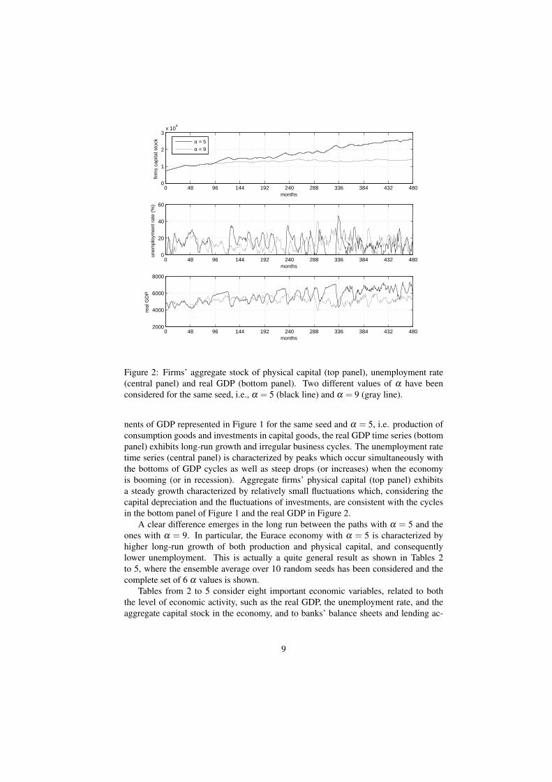
Figure 2 presents the typical simulation paths of the key real economic variables,i.e., the firms’ aggregate stock of physical capital (top panel), the unemployment rate(central panel) and the real GDP (bottom panel). For any of the three economic vari-ables considered, we represent the time path related to two different values of α , i.e.,α = 5 and α = 9. The time series have been represented ceteris paribus, including thesame seed of the pseudo-random number generator. Consistent with the two compo-

4The bankruptcy for insolvency occurs when the net worth of the firm becomes lower than zero. In thatcase, firm’ shareholders are wiped out and all workers are fired; the debt is also restructured and loans arepartially written-off in the lending banks’ portfolios; the firm’s physical capital is frozen and the firm remainsinactive as long as new financial capital is raised in the stock market.

8

0 48 96 144 192 240 288 336 384 432 4800

1

2

3x 10

4

months

firm

s ca

pita

l sto

ck

0 48 96 144 192 240 288 336 384 432 4800

20

40

60

months

unem

ploy

men

t rat

e (%

)

0 48 96 144 192 240 288 336 384 432 4802000

4000

6000

8000

months

real

GD

Pα = 5

α = 9

Figure 2: Firms’ aggregate stock of physical capital (top panel), unemployment rate(central panel) and real GDP (bottom panel). Two different values of α have beenconsidered for the same seed, i.e., α = 5 (black line) and α = 9 (gray line).

nents of GDP represented in Figure 1 for the same seed and α = 5, i.e. production ofconsumption goods and investments in capital goods, the real GDP time series (bottompanel) exhibits long-run growth and irregular business cycles. The unemployment ratetime series (central panel) is characterized by peaks which occur simultaneously withthe bottoms of GDP cycles as well as steep drops (or increases) when the economyis booming (or in recession). Aggregate firms’ physical capital (top panel) exhibitsa steady growth characterized by relatively small fluctuations which, considering thecapital depreciation and the fluctuations of investments, are consistent with the cyclesin the bottom panel of Figure 1 and the real GDP in Figure 2.

A clear difference emerges in the long run between the paths with α = 5 and theones with α = 9. In particular, the Eurace economy with α = 5 is characterized byhigher long-run growth of both production and physical capital, and consequentlylower unemployment. This is actually a quite general result as shown in Tables 2to 5, where the ensemble average over 10 random seeds has been considered and thecomplete set of 6 α values is shown.

Tables from 2 to 5 consider eight important economic variables, related to boththe level of economic activity, such as the real GDP, the unemployment rate, and theaggregate capital stock in the economy, and to banks’ balance sheets and lending ac-

9

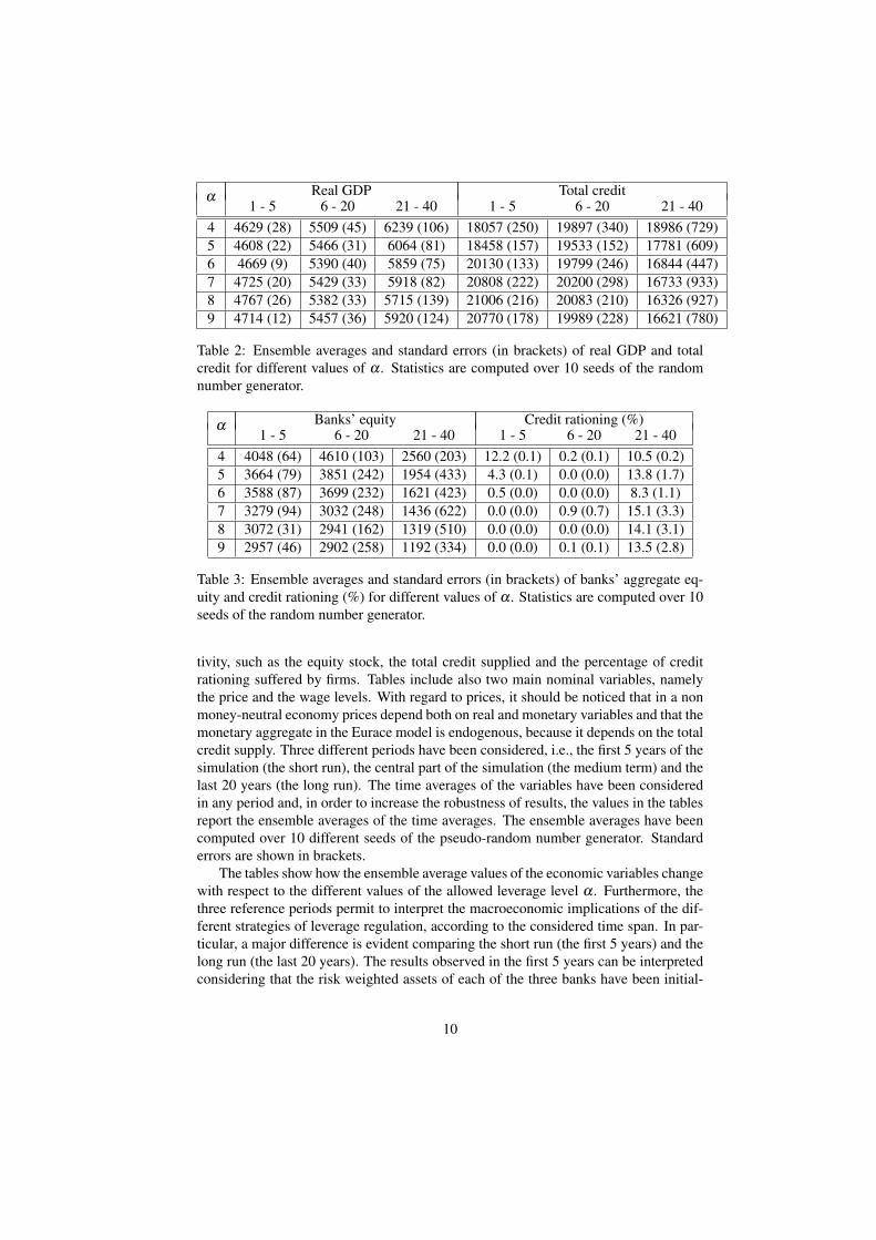
Real GDP Total creditα1 - 5 6 - 20 21 - 40 1 - 5 6 - 20 21 - 40

4 4629 (28) 5509 (45) 6239 (106) 18057 (250) 19897 (340) 18986 (729)5 4608 (22) 5466 (31) 6064 (81) 18458 (157) 19533 (152) 17781 (609)6 4669 (9) 5390 (40) 5859 (75) 20130 (133) 19799 (246) 16844 (447)7 4725 (20) 5429 (33) 5918 (82) 20808 (222) 20200 (298) 16733 (933)8 4767 (26) 5382 (33) 5715 (139) 21006 (216) 20083 (210) 16326 (927)9 4714 (12) 5457 (36) 5920 (124) 20770 (178) 19989 (228) 16621 (780)

Table 2: Ensemble averages and standard errors (in brackets) of real GDP and totalcredit for different values of α . Statistics are computed over 10 seeds of the randomnumber generator.

Banks’ equity Credit rationing (%)α1 - 5 6 - 20 21 - 40 1 - 5 6 - 20 21 - 40

4 4048 (64) 4610 (103) 2560 (203) 12.2 (0.1) 0.2 (0.1) 10.5 (0.2)5 3664 (79) 3851 (242) 1954 (433) 4.3 (0.1) 0.0 (0.0) 13.8 (1.7)6 3588 (87) 3699 (232) 1621 (423) 0.5 (0.0) 0.0 (0.0) 8.3 (1.1)7 3279 (94) 3032 (248) 1436 (622) 0.0 (0.0) 0.9 (0.7) 15.1 (3.3)8 3072 (31) 2941 (162) 1319 (510) 0.0 (0.0) 0.0 (0.0) 14.1 (3.1)9 2957 (46) 2902 (258) 1192 (334) 0.0 (0.0) 0.1 (0.1) 13.5 (2.8)

Table 3: Ensemble averages and standard errors (in brackets) of banks’ aggregate eq-uity and credit rationing (%) for different values of α . Statistics are computed over 10seeds of the random number generator.

tivity, such as the equity stock, the total credit supplied and the percentage of creditrationing suffered by firms. Tables include also two main nominal variables, namelythe price and the wage levels. With regard to prices, it should be noticed that in a nonmoney-neutral economy prices depend both on real and monetary variables and that themonetary aggregate in the Eurace model is endogenous, because it depends on the totalcredit supply. Three different periods have been considered, i.e., the first 5 years of thesimulation (the short run), the central part of the simulation (the medium term) and thelast 20 years (the long run). The time averages of the variables have been consideredin any period and, in order to increase the robustness of results, the values in the tablesreport the ensemble averages of the time averages. The ensemble averages have beencomputed over 10 different seeds of the pseudo-random number generator. Standarderrors are shown in brackets.

The tables show how the ensemble average values of the economic variables changewith respect to the different values of the allowed leverage level α . Furthermore, thethree reference periods permit to interpret the macroeconomic implications of the dif-ferent strategies of leverage regulation, according to the considered time span. In par-ticular, a major difference is evident comparing the short run (the first 5 years) and thelong run (the last 20 years). The results observed in the first 5 years can be interpretedconsidering that the risk weighted assets of each of the three banks have been initial-

10

Firms’ capital stock Unemployment (%)α1 - 5 6 - 20 21 - 40 1 - 5 6 - 20 21 - 40

4 9307 (20) 14881 (354) 20916 (880) 15.6 (0.6) 12.7 (0.4) 12.5 (0.3)5 9446 (33) 14128 (282) 19959 (677) 16.9 (0.5) 11.7 (0.5) 13.9 (0.5)6 9495 (12) 13690 (356) 17983 (638) 15.3 (0.2) 11.8 (0.5) 13.6 (0.6)7 9573 (23) 13802 (276) 18302 (577) 14.2 (0.4) 11.6 (0.3) 13.2 (0.5)8 9634 (26) 13414 (357) 16737 (1036) 13.5 (0.6) 11.5 (0.4) 13.1 (0.7)9 9575 (19) 13946 (325) 18489 (1000) 14.5 (0.3) 11.5 (0.3) 13.4 (0.5)

Table 4: Ensemble averages and standard errors (in brackets) of firms’ aggregate capitalstock and unemployment rate (%) for different values of α . Statistics are computedover 10 seeds of the random number generator.

Price index Wage levelα1 - 5 6 - 20 21 - 40 1 - 5 6 - 20 21 - 40

4 0.76 (0.00) 0.87 (0.02) 1.07 (0.03) 1.53 (0.02) 2.0 (0.05) 2.82 (0.11)5 0.76 (0.00) 0.84 (0.01) 1.05 (0.03) 1.53 (0.02) 1.88 (0.05) 2.74 (0.10)6 0.77 (0.00) 0.82 (0.01) 0.97 (0.02) 1.53 (0.01) 1.81 (0.04) 2.43 (0.09)7 0.78 (0.00) 0.83 (0.01) 0.98 (0.02) 1.54 (0.00) 1.83 (0.04) 2.47 (0.08)8 0.78 (0.00) 0.81 (0.02) 0.92 (0.04) 1.54 (0.00) 1.77 (0.06) 2.25 (0.14)9 0.78 (0.00) 0.83 (0.02) 0.98 (0.04) 1.55 (0.00) 1.86 (0.05) 2.51 (0.15)

Table 5: Ensemble averages and standard errors (in brackets) of aggregate price andwage levels for different values of α . Statistics are computed over 10 seeds of therandom number generator.

ized to be five times the initial level of equity. This implies that for values of α loweror equal to 5, the constraint on bank leverage is binding and it is not possible for banksin the short run to increase the supply of credit in order to match the demand by firms.The limitation of banks’ loans explains the high percentage values we observe for creditrationing in the first 5 years for α = 5 and in particular for α = 4, see Table 3, and theconsequent lower level of credit-money in the economy as observed in Table 2. Thelower level of credit supply reduces the opportunities for firms to invest, to increaseproduction and to hire new workers, and this is clearly evident in the short-run valuesof GDP, employment and firms’ capital stock which are the lowest for the values of αless or equal to 5 and increase more or less monotonically as α increases, see Tables 2and 4. On the contrary, the aggregate equity level of banks is monotonically decreas-ing with the leverage level α in the short run. In fact, in the case banks face a creditdemand higher than their supply constraints, as fixed by the institutional arrangements(α) and their equity level, they stop the payment of dividends to raise their net worthand to become able to meet the demand of credit in excess of supply.

The short run macroeconomic implications of the different values of α fade if themedium term time span is considered (years between 6 and 20) and disappear in thelong run. Indeed, it emerges that the short run implications are somehow reversedin the second half of the simulation, where we observe a better economic welfare on

11

average for the highest capital requirements (low values of α), and in particular forα = 4. The values of real GDP in table 2 actually show that lower capital requirementsdo not allow for economic expansion in the long run. We state that banks’ equity playsagain a crucial role in determining these findings. In fact, firms’ failures occurring inthe course of the simulation and the consequent debt write-offs reduce considerablythe equity of banks, see Table 3. Furthermore, the consequences of firms’ failure aremore severe when the value of α is high. The reasons is twofold: first in the case oflow capital requirements (high α), banks do not stop dividends’ payments, due to theabsence of credit rationing in the short run; therefore, they keep their net worth at theinitial relatively low levels; second, debt write-off are higher for more indebted firms,and firms’ indebtedness is higher for high α , due to the easier access to credit in theshort run. In fact, as it is clearly evident in Table 3, banks’ equity levels in case of lowercapital requirements are small in the first part of the simulation and are also subject tothe biggest reduction.

0 48 96 144 192 240 288 336 384 432 480−1000

0

1000

2000

3000

4000

5000

months

bank

s eq

uity

0 48 96 144 192 240 288 336 384 432 4800

0.5

1

1.5

2

2.5x 10

4

months

bank

s lo

ans

α = 5

α = 9

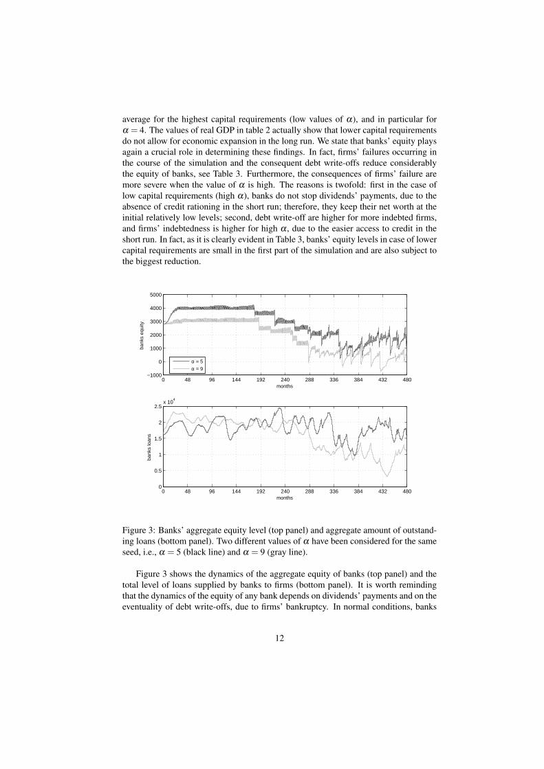
Figure 3: Banks’ aggregate equity level (top panel) and aggregate amount of outstand-ing loans (bottom panel). Two different values of α have been considered for the sameseed, i.e., α = 5 (black line) and α = 9 (gray line).

Figure 3 shows the dynamics of the aggregate equity of banks (top panel) and thetotal level of loans supplied by banks to firms (bottom panel). It is worth remindingthat the dynamics of the equity of any bank depends on dividends’ payments and on theeventuality of debt write-offs, due to firms’ bankruptcy. In normal conditions, banks

12

usually pay out all their profits as dividends to shareholders; however, in the case theBasel II-like institutional constraint set by α is binding, i.e., the demand for creditat a bank is higher than the allowed supply at the present equity level, then the bankstops dividends payments in order to increase its equity and thus being able to satisfythe entire loan demand in the future. This behavioral feature explains the increase inthe aggregate level of equity that is occurring in the case of low αs. In particular, it isworth noting the rise in the aggregate equity level that can be observed in the figure (toppanel) at the beginning of the simulation for α = 5, i.e., when the constraint is morebinding and therefore credit rationing is expected to occur. This effect can be examinedalso by looking at banks’ equity values of the first 5 years in table 3, considering thatbank’s equity is always initialized at a value close to 3000 (as shown also by figure3). The subsequent large drops of equity in figure 3 are therefore explained by firms’bankruptcy and consequent debt write-offs.

The dynamics of the aggregate amount of loans (bottom panel) is consistent withthe equity paths represented in the top panel, in particular whenever the demand forloans is rationed by insufficient levels of equity on the side of banks. In fact, at thebeginning of the simulation the aggregate amount of outstanding loans in the α = 5case is lower than the amount in the α = 9 case, consistently with the aggregate equityincrease occurring for α = 5 which indicates credit rationing. Furthermore, in thesecond part of the simulation, the higher amount of outstanding loans for α = 5 canbe explained by the lower severity of credit rationing in that case, as the higher equitylevel for α = 5 should clearly indicate.

Figure 4 shows the dynamics of two key nominal variables of the economy, i.e.,the price (top panel) and the wage level (bottom panel). The paths of the two variablesexhibit a general upward trend with some volatility, in particular for prices. It is worthnoting that the steepness of the upward trend depends on α and on the period consid-ered. In particular, in the short run the price and wage values are generally higher forα = 9, while in the long run the upward trend of prices and wages is clearly steeperfor α = 5. This result is consistent with the figures showed in the tables and with eco-nomic intuition, i.e., the dynamics of prices and wages positively depends on the oneof monetary aggregates and on the conditions of the real side of the economy.

Figure 5 shows in the top panel the dynamics of the monetary aggregate, i.e. theaggregate amount of liquid monetary resources in the Eurace economy, and presents inthe bottom panel the sum of the aggregate amount of outstanding loans and of centralbank liabilities. The monetary aggregate is defined at any time as the sum of all private(i.e., held by households and firms) and public (i.e., held by the Government and theCentral Bank) deposits plus banks’ equity. The initial value of the aggregate amountof outstanding loans is given by the sum of the debt of any firm, where firms’ debt hasbeen uniformly initialized so to have a leverage, i.e., a debt to book value of equityratio, equal to 2, considering also the assigned book value of assets. In real economiesthe amount of outstanding banknotes is part of the central bank liabilities. In Eurace,the initial value of central bank liabilities is defined as residual, i.e., as the differencebetween the initial value of the previously defined monetary aggregate and the initialaggregate amount of outstanding loans. The high-powered money provided by the cen-tral bank is therefore the part of the monetary aggregate not explained by banks’ loans.In absence of a quantitative easing policy performed by the central bank, i.e., if the cen-

13

0 48 96 144 192 240 288 336 384 432 480

0.7

0.8

0.9

1

1.1

1.2

months

cons

umpt

ion

good

s pr

ice

leve

l

0 48 96 144 192 240 288 336 384 432 4801.5

2

2.5

3

3.5

months

wag

e le

vel

α = 5

α = 9

Figure 4: Price level (top panel) ana wage level (bottom panel). Two different valuesof α have been considered for the same seed, i.e., α = 5 (black line) and α = 9 (grayline).

tral bank does not inflate its balance sheet by purchasing government bonds, as it is thecase for the results presented in this study5, central bank liabilities has to be consideredconstant, and the variation of the monetary aggregate should be eventually explainedonly by the dynamics of the aggregate amount of outstanding loans. Figure 5 confirmsthe above argument, as the time value of the monetary aggregate (top panel) is identicalto the time series presented in the bottom panel, i.e., to the value of outstanding loansplus central bank liabilities, the latter to be considered constant in the simulations. Thisresult further corroborates the rationale behind the theory of endogenous money. Thedifferent behavior observed with respect to the two values of α is consistent with thefigures presented in the tables and with previous considerations. In particular, the val-ues of the monetary aggregate and its counterpart, i.e. the aggregate outstanding loansplus the central bank liabilities, are characterized by higher values in the short run forα = 9, while in the long run the situation is reversed and the time series referred toα = 5 dominate.

The clear evidence of results presented in this study is that the monetary aggregateplays a key role in determining the real variables of the economy. Furthermore, the

5A study about the effects of quantitative easing in the Eurace economy can be found in Cincotti et al.2010 [14].

14

0 48 96 144 192 240 288 336 384 432 4801

1.5

2

2.5

3

3.5x 10

4

months

Agg

reat

e pr

ivat

e an

d pu

blic

sec

tor

depo

sits

0 48 96 144 192 240 288 336 384 432 4801

1.5

2

2.5

3

3.5x 10

4

months

Ban

ks c

redi

t−m

oney

+ C

B fi

at m

oney

α = 5

α = 9

Figure 5: Aggregate amount of liquid monetary resources (top panel) and aggregateamount of outstanding loans plus central bank liabilities (bottom panel). Two differentvalues of α have been considered for the same seed, i.e., α = 5 and α = 9.

monetary aggregate is made by two components, an endogenous one, or endogenousmoney, which is given by the aggregate outstanding loans created by the banking sec-tor, and an exogenous one which is set by the monetary authorities, i.e., by the centralbank. The first component should be considered as endogenous because is determinedby the self-interested interaction of private agents, i.e., banks and firms, while the sec-ond component can be considered as exogenous because may depend on discretionaryunconventional monetary policies, like quantitative easing. The rate of growth andlong-run dynamics of endogenous money, however, depends also on parameters or in-stitutional constraints, like α , which can be considered as exogenous because set by theregulatory authorities. Actually, the main result of the paper regards the role of a policysetting, like banks’ capital adequacy ratio, on the dynamics of endogenous money andtherefore on the growth of the economy.

Investigating the role played by the monetary aggregate in the real economy hasbeen the subject of research in economics for many years and is still the topic of a widedebate, as testified by the controversy between endogenous and exogenous money the-orist [9, 17, 18]. In this paper, we limit to point out an interesting similarity betweenEurozone economic data and Eurace data concerning the cross-correlation between thepercentage variations of GDP and percentage variations of M3, as shown in figure 6.

15

The left panel shows the cross-correlation diagram between the percentage variationsof real GDP, shown in Figure 2 (bottom panel), and the monetary aggregate, shownin Figure 5 (top panel), both for α = 5. The right panel presents again the cross-correlation diagram computed now considering the percentage variations of Eurozonereal GDP and the percentage variation of a broad measure of the monetary base, theso-called M3. Eurozone cross-correlation diagram has been computed on a quarterlybase, contrary to the Eurace case, where data are all macroeconomic data are conven-tionally generated on a monthly time scale. In fact, Eurone GDP are provided on aquarterly base, therefore also M3 data, which are recorded on a monthly base, has beentransformed to a quarterly time series, by considering the quarterly average. EurozoneGDP data are working day and seasonally adjusted as well as chain-linked to adjustfor inflation with the 2000 as reference year. Eurozone GDP data refers to the period Iquarter 1995 - IV quarter 2010, while M3 data to the period January 1995 - December2010. All data are available on Internet at the European Central Bank statistical datawarehouse6.It is worth noting that, apart the different time scales involved, the two cross-correlationdiagrams are characterized by a similar pattern, as in both cases the percentage vari-ations of real GDP lead the percentage variations of the monetary aggregate. Thisfinding further confirm the rationale behind the theory of endogenous money, statingthat the stock of money is determined by the demand for bank credit, which is in turninduced by the economic variables that affect the GDP.

3 ConclusionsAfter start of the global financial crisis in 2007, an increasing attention has been de-voted to the design of proper regulation systems of the banking sector. A great efforthas been done in order to understand and foresee the consequences of different regu-lation strategies on the stability of the financial system, on growth, and on the mainmacroeconomic variables. As pointed out in the introduction, many reports on thistopic are available, mainly produced by central banks research centers or by interna-tional organizations. One of the central themes is the assessment of the long-termimpact of different capital requirements for banks. The methodology is typically basedon a set of economic models that originate in the DSGE class, which are estimated orcalibrated according to data sets belonging to specific countries or areas.

The aim of this paper is to tackle the same topic using an agent-based approach. TheEurace model provides with a complex economic environment where to run computersimulations and to perform what-if analysis related to policy issues. The model hasbeen calibrated by using realistic empirical values both for the parameters of the modeland for the state variables initialization.

Capital adequacy ratio, i.e., the ratio between banks’ equity capital and risk-weightedassets, has been chosen as the key varying parameter that assumes six different values.For each value a set of ten simulations with different random seeds has been run, andthe results have been reported and analyzed.

6http://sdw.ecb.europa.eu

16

−20 −15 −10 −5 0 5 10 15 20−0.4

−0.3

−0.2

−0.1

0

0.1

0.2

0.3

0.4

0.5

Sam

ple

cros

s co

rrel

atio

n

Lag (months)

EURACE

−20 −15 −10 −5 0 5 10 15 20−0.4

−0.3

−0.2

−0.1

0

0.1

0.2

0.3

0.4

0.5

Sam

ple

cros

s co

rrel

atio

n

Lag (quarters)

Eurozone

Figure 6: Cross-correlation diagram between Eurace real GDP and monetary aggregatedata (left panel) and between Eurozone real GDP and M3 data. The dashed symmetricbounds refers to the 95 % confidence level interval for the sample cross-correlationunder the null hypothesis of zero theoretical cross-correlation. The bounds values aregiven by ± 2√

N, where N is the sample size. This explains the difference between the

left panel bounds, where we have 480 monthly data, i.e., 40 years of simulation, andthe Eurozone case (right panel) characterized by only 64 quarterly data, i.e., the 16years from 1995 to 2010.

The outcomes of the models consist of time series that are characterized by quiterealistic graphical patterns. In particular long-run growth and endogenous businesscycles are observed. The capital adequacy ratio proved to have significant macroeco-nomic implications that depend critically on the considered time horizon.

In the short run (up to five years) a lower leverage policy, restricting the creditsupply, has negative macroeconomic consequences, reducing growth, investments andemployment. Actually, the limited credit supply determines firms’ rationing, whereas ahigher leverage allows firms to get loans without incurring in credit rationing. However,the higher debt load that firms acquired in the short run in the case of less restrictivepolicies, i.e., low capital adequacy ratio, turns out to have significative implicationsif considered along with the lower equity capital of banks. Indeed, in the case oflow capital adequacy ratio, firms financial fragility becomes higher and consequentlyfirms bankruptcies are more frequent. These bankruptcies undermine the equity capital

17

of banks, that in the case of high leverage has not been sufficiently raised by banks,determining a severe reduction of the lending capacity of the banking sector in thelong run. On the other hand, if capital adequacy ratio is higher, firms experience lessopportunities to increase production and hire new workers in the short run, but later,due to the higher equity of banks, that needs to raise it by retaining dividends in orderto face the credit demand, the banking system proves to be more stable, with lowervalues of credit rationing and a higher level of total loans.

According to the outcomes of the Eurace model, the credit dynamics markedlyinfluences the macroeconomic activity. The banking system is therefore crucial, andan appropriate set of regulations seem to have great potential benefits for growth andeconomic stability. The model we presented reproduces in detail the interaction amongeconomic agents, and shows that it can already be effectively used as an environmentwhere performing economic analysis and forecast, and where testing policy strategies.

AcknowledgementThis work was carried out in conjunction with the Eurace project (EU IST FP6 STREPgrant: 035086) which is a collaboration lead by S. Cincotti (Università di Genova), HDawid (Universitaet Bielefeld), C. Deissenberg (Université de la Méditerranée), K.Erkan (TUBITAK-UEKAE National Research Institute of Electronics and Cryptol-ogy), M. Gallegati (Università Politecnica delle Marche), M. Holcombe (Universityof Sheffield), M. Marchesi (Università di Cagliari), C. Greenough (Science and Tech-nology Facilities Council Rutherford Appleton Laboratory).

References[1] Basel ii: International convergence of capital measurement and capital standards:

A revised framework - comprehensive version. Technical report, BIS, Basel Com-mittee on Banking Supervision, 2006.

[2] Eurace Final Activity Report. Technical report, Eurace Project, 2009.

[3] An assessment of the long-term economic impact of stronger capital and liquidityrequirements. Technical report, BIS, Basel Committee on Banking Supervision,2010.

[4] Interim report on the cumulative impact on the global economy of proposedchanges in the banking regulatory framework. Technical report, Institute of Inter-national Finance, 2010.

[5] Strengthening international capital and liquidity standards: A macroeconomicimpact assessment for canada. Technical report, Bank of Canada, 2010.

[6] Anat R. Admati, Peter M. DeMarzo, Martin F. Hellwig, and Paul Pfleiderer. Fal-lacies, irrelevant facts, and myths in the discussion of capital regulation: Why

18

bank equity is not expensive. Working Paper Series of the Max Planck Institutefor Research on Collective Goods 2010-42, Max Planck Institute for Research onCollective Goods, September 2010.

[7] Tobias Adrian and Hyun Song Shin. Liquidity and leverage. Journal of FinancialIntermediation, 19(3):418–437, July 2010.

[8] Paolo Angelini, Laurent Clerc, Vasco Curdia, Leonardo Gambacorta, AndreaGerali, Alberto Locarno, Roberto Motto, Werner Roeger, Skander Van denHeuvel, and Jan Vlcek. Basel iii: Long-term impact on economic performanceand fluctuations. Questioni di economia e finanza, Banca d’Italia, 2011.

[9] Philip Arestis and Malcolm Sawyer. The nature and role of monetary policywhen money is endogenous. Cambridge Journal of Economics, 30(6):847–860,November 2006.

[10] Allen N. Berger, Richard J. Herring, and Giorgio P. Szego. The role of capitalin financial institutions. Journal of Banking & Finance, 19(3-4):393–430, June1995.

[11] Jurg Blum and Martin Hellwig. The macroeconomic implications of capital ad-equacy requirements for banks. European Economic Review, 39(3-4):739–749,April 1995.

[12] Ricardo J Caballero. A fallacy of composition. American Economic Review,82(5):1279–92, December 1992.

[13] Ricardo J. Caballero. Macroeconomics after the crisis: Time to deal with thepretense-of-knowledge syndrome. Journal of Economic Perspectives, 24(4):85–102, Fall 2010.

[14] Silvano Cincotti, Marco Raberto, and Andrea Teglio. Credit money andmacroeconomic instability in the agent-based model and simulator Eurace.Economics: The Open-Access, Open-Assessment E-Journal, 4(26), 2010.http://dx.doi.org/10.5018/economics-ejournal.ja.2010-26.

[15] H. Dawid, S. Gemkow, P. Harting, and M. Neugart. Spatial skill heterogeneityand growth: an agent-based policy ananlysis. Journal of Artificial Societies andSocial Simulation, 12(4), 2009.

[16] Herbert Dawid, Michael Neugart, Klaus Wersching, Kordian Kabus, Philipp Hart-ing, and Simon Gemkow. Eurace Working Paper 7.1: Capital, ConsumptionGoods and Labor Markets in Eurace. Technical report, Bielefeld University, april2007.

[17] G. Fontana. Post keynesian approaches to endogenous money: a time frameworkexplanation. Review of Political Economy, 15:291–314, 2003.

[18] W. Godley and M. Lavoie. Monetary Economics: An Integrated Approach toCredit, Money, Income, Production and Wealth. Palgrave Macmillan, 2007.

19

[19] Martin Hellwig. Capital regulation after the crisis: Business as usual? Workingpaper series of the max planck institute for research on collective goods, MaxPlanck Institute for Research on Collective Goods, July 2010.

[20] Katarina Juselius and Massimo Franchi. Taking a dsge model to the data mean-ingfully. Economics: The Open-Access, Open-Assessment E-Journal, 1(2007-4),2007.

[21] Peter Kriesler and Marc Lavoie. The new consensus on monetary policy and itspost-keynesian critique. Review of Political Economy, 19(3):387–404, 2007.

[22] S. Myers and N.S. Majluf. Corporate financing and investment decisions whenfirms have information that investors do not have. Journal of Financial Eco-nomics, 13(2):187–221, June 1984.

[23] A. Teglio, M. Raberto, and S. Cincotti. Balance sheet approach to agent-basedcomputational economics: the EURACE project, volume 77 of Advances in Intel-ligent and Soft Computing, pages 603–610. Springer Verlag, 2010.

[24] A. Teglio, M. Raberto, and S. Cincotti. Endogeneous credit dynamics as source ofbusiness cycles in the Eurace model, volume 645 of Lecture Notes in Economicsand Mathematical Systems, pages 203–214. Springer Verlag, 2010.

[25] L. Tesfatsion and K. Judd. Agent-Based Computational Economics, volume 2 ofHandbook of Computational Economics. North Holland, 2006.

20