This article was downloaded by: [Stanford University Libraries]On: 15 February 2012, At: 19:00Publisher: RoutledgeInforma Ltd Registered in England and Wales Registered Number: 1072954 Registeredoffice: Mortimer House, 37-41 Mortimer Street, London W1T 3JH, UK

Education EconomicsPublication details, including instructions for authors andsubscription information:http://www.tandfonline.com/loi/cede20

The Identification of School ResourceEffectsEric. A Hanushek a , Steven. G Rivkin b & Lori. L Taylor ca University of Rochester, Wallis Institute of Political Economy,Rochester, NV, 14627-0158, USA E-mail:b Department of Economics, Amherst College, Amherst, MA,01002, USA E-mail:c Research department, Federal Reserve Bank of Dallas, StationK, Dallas, TX, 75222, USA E-mail:

Available online: 28 Jul 2006

To cite this article: Eric. A Hanushek, Steven. G Rivkin & Lori. L Taylor (1996): The Identificationof School Resource Effects, Education Economics, 4:2, 105-125

To link to this article: http://dx.doi.org/10.1080/09645299600000012

PLEASE SCROLL DOWN FOR ARTICLE

Full terms and conditions of use: http://www.tandfonline.com/page/terms-and-conditions

This article may be used for research, teaching, and private study purposes. Anysubstantial or systematic reproduction, redistribution, reselling, loan, sub-licensing,systematic supply, or distribution in any form to anyone is expressly forbidden.

The publisher does not give any warranty express or implied or make anyrepresentation that the contents will be complete or accurate or up to date. Theaccuracy of any instructions, formulae, and drug doses should be independently verifiedwith primary sources. The publisher shall not be liable for any loss, actions, claims,proceedings, demand, or costs or damages whatsoever or howsoever caused arisingdirectly or indirectly in connection with or arising out of the use of this material.

Education Economics, Vol. 4, No. 2, 1996

The Identification of School Resource Effects

ERIC A. HANUSHEK, STEVEN G. N V I a N & L O N L. TAYLOR

ABSTRACT In the US, the federal government plays a relatively minor role in setting school policy, and the separate states are an important source of policy variation that sets the environment faced by local school districts. The variation in state policies plausibly has a significant impact on student achievement. Little is known about the magnitude of such effects, because data limitations have seldom allowed researchers to specify fully the state policy environment when analyzing school effects. Dzfferences in overall school policies may, however, help to reconcile the contradict0 y findings about the effectiveness of school resource usage that exist. We develop a simple theoretical model demonstrating that the bias induced by omitting relevant state characteristics is greater in state-level analyses than it is in less aggregate studies. Our exploration of aggregation bias using the High School and Beyond data set suggests that aggregation to the state level inflates the coeficients on school input variables. Moreover, the results do not support the competing hypothesis that aggregation is beneficial because it reduces biases from measurement error. These results are completely consistent with the findings of production function studies where positive school resource effects an achievement are much much likely to be found when estimation involves state-level data.

Introduction

A wide variety of US state policies plausibly impact measured student achievement. The separate states determine the ages for compulsory school attendance, the curriculum requirements for high-school graduation, the extent and character of student competency exams, and the certification requirements for primary and secondary school teachers. They set school financing formulae, fund public universities and choose textbooks. Less directly, the states choose state tax and welfare policies that alter the expected costs and benefits of schooling. Unfortu- nately, data limitations seldom allow researchers to specify fully the state policy environment when analyzing school effects. Therefore, problems of omitted vari-

E. A. Hanushek, University of Rochester, Wallis Institute of Political Economy, Rochester, NY 14627-0158, USA. S. Rivkin, Amherst College, Department of Economics, Amherst, MA 01002, USA. L. Taylor, Federal Reserve Bank of Dallas, Research Department, Station I<, Dallas, T X 75222, USA. E-mail: hanu(</ troi.cc.rochester.edu, rivkinitr acesgr.econ.amherst.edu and Lori_L_Taylor(ir frb-main- 5.ccmail.cornpuserve.com. We would like to thank Julian Betts, Jeff Grogger, Robert Willis, Geoffrey Woglom and participants at the NSFIReview of Economics and Statistics conference on 'School Quality and Educational Outcomes' (Haward University, December 1994) for helpful comments. An expanded theoretical development plus extension of the empirical results to multiple outcomes is found in Hanushek et al. (1996).

0964-5292/96/020105-2 1 1 1996 Journals Oxford Ltd

Dow

nloa

ded

by [

Stan

ford

Uni

vers

ity L

ibra

ries

] at

19:

00 1

5 Fe

brua

ry 2

012

106 E. A. Hanushek et al.

ables bias are inevitable. More important, certain estimation strategies may worsen the biases, leading to misleading interpretations of research into school policy.

We link these specification problems directly to the controversies about the effectiveness of school resources. A growing body of research casts doubt on the effectiveness of local school districts at turning added resources into higher student achievement. In comprehensive summaries of the empirical evidence, Hanushek (1986, 1989) found that there was no consistent or systematic relationship between achievement and either pupil-teacher ratios, teacher salaries, years of teacher schooling, years of teacher experience or per-student expenditure. The inefficacy of smaller pupil-teacher ratios is particularly noteworthy, given that the widely held belief that lower pupil-teacher ratios improve educational outcomes has played a prominent role in the crafting of educational policies. But these conclusions are not universally accepted. Some argue that the use of standardized test scores as the measure of achievement in most research ignores the potential impact of smaller class sizes or higher teacher salaries on other educational outcomes. Two widely cited recent studies by Card and Krueger (1992a,b) provide evidence that smaller classes and higher teacher salaries increase the wage premium associated with an additional year of schooling. The apparent conflict of wage studies and education production functions has inspired extensive efforts to reconcile the results (e.g. Burtless, 1996).'

This paper highlights the influence that aggregation and model specification has had on studies of educational performance. Educational production functions concentrate on the relationship between student outcomes and individual school and school district characteristics, while most wage analyses, including Card and Krueger, use state average school characteristic^.^ We present a statistical model demonstrating that the bias induced by omitting data on relevant state policies is greater in such state-level analyses than in more disaggregated studies. The model suggests that aggregation to the state level inflates the apparent impact of school resources.

Using the High School and Beyond (HSB) data set, we estimate aggregated and disaggregated relationships between the primary determinants of school expenditures (teacher-pupil ratios and teacher salaries) and one measure of educational outcomes (years of post-secondary schooling). Our analysis finds that aggregation to the state level inflates the estimated importance of school characteristics. More importantly, the pattern of results is consistent with an aggregation-induced increase in omitted variables bias and is not consistent with an errors-in-variables explanation.

Finally, we present data from past analyses to educational production functions on the importance of aggregation. A stylized fact that emerges from past analysis is that aggregation inflates the apparent significance of school resources. The fundamental underlying cause appears to be omission of key state policies from the estimation that is worsened by aggregation.

Variations in State Policy

T o motivate the subsequent development, some understanding of the central importance of state education policies is necessary. State policies potentially affecting measured student achievement can be classified into three broad catego- ries. First, finance policies directly affect the level of school resources and the degree of local control over school spending. Second, states directly intervene in the delivery of education through operating regulations, hiring .and personnel restrictions, and other process requirements for schools. Finally, other policies

Dow

nloa

ded

by [

Stan

ford

Uni

vers

ity L

ibra

ries

] at

19:

00 1

5 Fe

brua

ry 2

012

School Resource Eflects 107

Table 1. Current expenditures per pupil for the 1990- 1991 school year, by state

MD, PA, VT MA, RI DE, IL, MI, NH, OR, WI, WY CO, FL, HI, ME, MN, MT, NE, OH, WA IN, IA, KS, MO, NV, VA, WV AZ, CA, GA, I-, LA, NC, ND, SC, TX AL, AR, NM, OK, SD, T N ID, MS UT

Source: US Department of Education (1993).

Table 2. Unweighted distribution of state expenditures for public primary and secondary education

Standard School year Mean deviation Minimum Maximum

Total current expenditures (1990-1991 US$) 1990-1991 5155 1291 1979-1980 3824 97 1

1969-1970 2727 566 1959-1960 1634 369

Local share of total revenues" 1990-1991 42.1 16.2 1979-1980 42.2 16.5 1969-1970 50.2 17.7 1959-1960 53.0 20.4

"Includes revenue from tuition and fees. Source: US Department of Education (1993).

influence measured student achievement by influencing the characteristics of the student body, either directly through regulations on compulsory attendance or indirectly through their effect on the perceived costs and benefits of schooling.

School finance formulae in common usage differ in both form and detail (Gold et al., 1992). As of the 1990-1 99 1 school year, 38 states guaranteed to local school districts a minimum level of funding per pupil (i.e. foundation grants). The remaining states relied primarily on either flat grants to local school districts (Delaware and North Carolina), matching grants (Kansas, Massachusetts, Michi- gan, New York, Pennsylvania, Rhode Island and Wisconsin) or a system of full state funding (Hawaii and Washington). All of these formulae, however, use different aid parameters and have different implications for the local price of schools.

Given the wide variety of financing formulae, it is not surprising that expendi- tures per pupil also vary widely among the states. As Table 1 illustrates, total current expenditures in 1990 varied from less than US$3000 per pupil in Utah to more than US$8000 per pupil in New Jersey and New York (US Department of Education, 1993). As a general rule, expenditures per pupil were nearly 20% lower

Dow

nloa

ded

by [

Stan

ford

Uni

vers

ity L

ibra

ries

] at

19:

00 1

5 Fe

brua

ry 2

012

108 E. A. Hanushek et al.

in states that relied on foundation grants than they were in states that relied on other finance strategies.

Furthermore, as Table 2 indicates, wide variation in expenditures among the states is not a recent phenomenon. Total current expenditures per pupil during the 1959-1960 school year ranged from US8938 in Mississippi to over US82500 in New York (in constant 1990-1991 US$). Data for the 1969-1970 and 1979-1980 school year show a similarly wide range of expenditures.

The variety of school finance formulae also give rise to a dramatic variation in the extent to which school districts exert local control over the size of their budgets (Table 2). For the 1990-1 99 1 school year, local financing ranged from negligible local funding in Hawaii to nearly total local funding in New Hampshire. Researchers have postulated that the extent of local control over the schools influences school effectiveness by influencing the extent of community monitoring of the schools.

While the various school finance formulae affect the amount of resources available to schools, a large number of additional state policies affecting the operation of the schools may be more important for our purposes here. Two of the most common state policies of this type are curriculum requirements for high- school graduation and minimum competency tests for teachers and students (US Department of Education, 1993). These are reinforced by a variety of direct and indirect operating regulations. The wide policy variation introduces systematic and potentially important differences in the operations of schools.

Other potentially important state policies affect the composition of the student body rather than the funding and operation of the schools. For example, if we assume that students are more likely to drop out of the lower tail of the achievement distribution, then variations in the age at which students can legally leave school can have considerable influence on the characteristics of the student body at the high school level. States that allow students to leave school at an earlier age would tend to retain fewer students who would score low on standardized tests. Therefore, state rules on compulsory attendance can have a strong influence on measured student a~hievement .~

Other state policies influence the perceived costs and benefits of schooling. For example, there is considerable variation in tax and welfare policy among the states. In 1990, state income tax rates ranged from zero in the seven states without an income tax (Alaska, Florida, Nevada, South Dakota, Texas, Washington and Wyoming) to over 10% for certain residents of Montana and North Dakota (US Bureau of the Census, 1992). Average weekly unemployment benefits ranged from US$102 in Louisiana to US8217 in Massachusetts, while average monthly pay- ments for Aid to Families with Dependent Children (AFDC) ranged from US812 1 in Alabama to US8720 in Alaska (US Bureau of the Census, 1992).

For our purposes, the key element is the variation in school funding and policy and in other relevant state factors. These factors, which are likely to be correlated with observed attributes of schools in each state, will bias estimated school effects that come from cross-state variations in resources. While this bias may be relatively small when analyzing achievement in individual classrooms and schools, its importance will increase with aggregation to state-level performance.

Model

We model the relationship between educational attainment and student and family characteristics as

Dow

nloa

ded

by [

Stan

ford

Uni

vers

ity L

ibra

ries

] at

19:

00 1

5 Fe

brua

ry 2

012

School Resource Efects 109

where Aij is the level of educational achievement for individual i in school j, Tij is a standardized pre-test score, Fij is a vector of individual and family characteristics. Cij is a vector of community variables and Sij is a vector of school characteristics.

Adequate controls for differences in family background, community environment and student preparation are needed in order to isolate the effects of school characteristics. Education goes on both inside and outside schools. The performance of any specific student will combine the influences of the shcool and of the outside environment, particularly the family. Moreover, parents may systematically select school districts through migration in accordance with their preferences (Tiebout, 1956) or otherwise attempt to secure good school resources for their children. In such a case, unmeasured parental inputs could be correlated with measured school resources.

Accounting for pre-existing differences in academic preparation is necessary in order to capture the impact of school factors during a given period. Education occurs over time, so that the achievement, say, of a ninth grader is determined in part by schools (and family) in the ninth grade and in part by these inputs in prior years. Since data on the past history of educational inputs are frequently not available, strategies that will isolate the achievement gains that might be related to specific measured inputs such as through estimation of value-added models of achievement are often employed (see, for example, Hanushek, 1979; Aitkin & Longford, 1986; Hanushek & Taylor, 1990).

One concern in modeling the educational processes involves simultaneity biases resulting from schools using past student performance in determining input allocations (e.g. lower class size for poorly performing students). The econometric problems arise when the unmeasured errors in the school attainment equation are correlated with the school inputs through school decision-making. While this may be legislated in other countries (see Mayston, 1996), no simple pattern exists in the US where compensatory programmes, gifted programmes and local demands play against each other. Such possible decision-making effects, however, reinforce the need to control for past performance in analyzing the effects of school resources; to the extent that any allocation decisions are captured by observed earlier performance, any such biases will be small.4

General estimation issues in the analysis of educational production functions pervade the discussion here. Clearly, inadequate controls for academic preparation, family inputs and the like will bias the estimated effects of school characteristics on achievement. At the same time, virtually no attention has been given to how aggregation of data might interact with such specification bias. We develop a conceptual model that shows how aggregation can affect the magnitude of any omitted variables bias and then subject it to empirical analysis.

Aggregation and the Sources of Bias

Virtually all discussion of aggregation of models, measurement errors and omitted variables is conducted in the context of a simple linear model. While some have suggested that such models are inappropriate in many of the educational circum- stances investigated here, we neglect consideration of non-linearities and concentrate on the other issue^.^

The level of aggregation can influence the estimated relationship between educational outcomes and specific school characteristics in a number of ways.6

Dow

nloa

ded

by [

Stan

ford

Uni

vers

ity L

ibra

ries

] at

19:

00 1

5 Fe

brua

ry 2

012

1 10 E. A. Hanushek et al.

This section examines aggregation related issues in the simplest form using regression equation (2):

where the subscript s indexes state of residence, Fijs, Cijs and Sij, are single measures summarizing the relevant inputs of family, community and school for individuals i, and eijs is an iid random error.

Most studies of educational production functions implicitly assume that t,hijs is invariant across individuals, schools and state of residence. In other words, the marginal impact of a change in a school characteristic like per-pupil expenditure is the same regardless of socio-economic background, academic skill or even the value of school expenditure itself: t j i j , = I) for all 2, j and s. Under such conditions, aggregation to the district or state level will not alter the estimated relationship between attainment and school expenditure (although the form of the data will generally affect the efficiency of the estimates).

Unfortunately, equal marginal effects for all students is a sufficient condition for perfect aggregation only when the empirical model is correctly specified. In practice, information for certain relevant variables might be unavailable. If the omitted variables are correlated with included school characteristics, then the estimated school coefficients will be biased regardless of the level of aggregation.

The magnitude of omitted variable bias depends on both the coefficient on the omitted variable and the coefficients on the included school characteristics from auxiliary regressions of the omitted variable on the included school characteristics. If aggregation alters any of these coefficients, it will change the size of the bias and thus the estimated relationship between attainment and school inputs. Unfortu- nately, there is no general rule to indicate whether aggregation will increase or decrease the size of the omitted variables bias (for more discussion, see Hanushek et al., 1996). However, aggregation to the state level necessarily increases omitted variable bias when the omitted variables are determined at the state level (with no within-state variation).

Aggregation and Omitted Variables in a Two-variable Model

Equation (3) presents a simplified version of equation (2) that ignores all variation in pre-test scores and family backgrounds, assumes that Sjs represents a single measure of school quality common to all students in school j and subsumes the influence of all community factors into a single, state-level measure of community environment (C,).' By assumption, the marginal impacts of both school expendi- ture and community environment are identical for all students:

If there is no information on the relevant aspects of community environment, a regression of academic attainment on school expenditure will produce the follow- ing biased estimate of the school expenditure coefficient:

where $ equals the school expenditure coefficient in an auxiliary regression of community environment on school expenditure. Even if equation (3) satisfies the conditions for perfect aggregation, aggregation will alter the bias in the estimate of $ through its impact on the coefficient 4.

Dow

nloa

ded

by [

Stan

ford

Uni

vers

ity L

ibra

ries

] at

19:

00 1

5 Fe

brua

ry 2

012

School Resource Efects 1 1 1

The effects of aggregation on the coefficient 4 are analyzed assuming that both C and S are driven by a common underlying factor, A, which indexes, say, tastes for education. With a linear specification and the assumption that only state-level values of A effect the community environment, we can write Cs and Sjs as

Sjs = y (A,, - A,) + 6As + Vjs (6)

where the bar indicates the state average for A. We allow both local and state values of A to affect school expenditure, reflecting the influence of both the state and local political processes in determining school characteristics.' We define C,, Aj, and As so that t, y and 6 are all non-negative, and restrict 6 to be greater than y so that school expenditures do not fall as As rises. U, and I/,, are iid random errors that are independent of each other and the variable A.

The coefficient 4 equals the covariance of C and S divided by the variance of S. Using equations 5 and 6, this equals

where the variances of A and V (02) have been partitioned into within-state (subscript w) and between-state (subscript 6) components.

When the data are aggregated to the state level, equation 6 is rewritten as

l and 4, the aggregate auxiliary regression coefficient, equals

By comparing equations (7) and (9), it is clear that 4 < 4. Thus, the aggregate estimate of $ is unambiguously biased upwards from the micro-level estimates.

Measurement Error

T o this point, we have assumed that the school characteristics are measured without error. An alternative concern about the estimation of school performance models is the possibility of measurement error in the school variable. If data are collected by surveys, their quality may be low when the local respondent is uncertain about the precise values, say, of expenditure or even number of students. On a related issue, if the educational models are aggregated over time instead of employing the basic value-added formulation sketched in equations (1) and (2), year-to-year fluctuations in the data may provide a misleading picture of the relevant historical data.9 In other words, measurement error is likely to be particularly important as empirical specifications diverge from the ideal described in equation (1).

The effect of measurement error in simple linear models is well-known (see, for example, Maddala, 1977, pp. 292-300).1° If the observed school input is

Dow

nloa

ded

by [

Stan

ford

Uni

vers

ity L

ibra

ries

] at

19:

00 1

5 Fe

brua

ry 2

012

1 12 E. A. Hanushek et al.

then the estimate of $ will be inconsistent and biased towards zero, even when v is iid with mean zero. The coefficients for other variables in the model (measured without error) will also be biased, but the direction of bias is ambiguous.

An important aspect of random measurement error is that aggregation within defined groups (e.g. states) can lessen the bias from measurement error under certain circumstances (Maddala, 1977). Grouping effectively reduces bias as long as the grouping strategy preserves between-group differences in the value of the regressor. Employing stage average differences in school characteristics suggests that aggregation by state would reduce the downward bias of any measurement error and potentially increase the parameter estimates.

None the less, theory alone cannot determine whether aggregation reduces a downward bias present in school-level studies or introduces an upward bias that inflates school resource coefficients in more aggregate analyses. This indeterminacy leads us to examine aggregation empirically within the context of state variations in educational performance. The effects of school resources on schooling attain- ment are considered at both the school level and the state level to investigate aggregation within a consistent model specification and data source.

Data

Data for the empirical analysis come from the HSB longitudinal survey. In 1980, a baseline survey provided data from approximately 36 high-school seniors from close to 1000 high schools. The base year survey reports parental schooling and income, contains information on the high schools, and provides scores for a battery of standardized mathematics, verbal and science tests. Follow-up surveys com- pleted in 1982, 1984 and 1986 provided post-high-school information on school and labor market attainment.

We concentrate on student outcomes measured by years of post-secondary schooling attained within 6 years of graduation for high-school graduates. It varies from zero (no post-secondary schooling) to eight (a PhD, MD, etc.). We use the 12th grade test score as the pre-test in order to isolate the contribution of high schools to post-secondary schooling. This implies that any impact of high schools on post-secondary schooling is additional to their effects on cognitive achievement.

The vector Fij includes race, gender, parental schooling and family income. Measured characteristics of C i j include the percentage of community residents who have a college degree, the local unemployment and wage rates for high-school graduates, the resident tuition at state universities, and indicator variables if the school is located in the south or in a rural area. Both local and state aggregates of community factors are analyzed. The percentage of college-educated residents captures environmental effects on educational expectations and achievement. Local wages and unemployment rates reflect variations in the opportunity cost of attending college, while the state resident tuition at public universities indexes the monetary cost of college attendance.14

These community variables reflect direct economic factors affecting college attendance, but they do not capture the larger state policy influences motivating this paper. Therefore, to the extent that further factors are omitted, as we believe to be the case, the models still yield biased coefficient estimates and are subject to the problems identified here. The consideration of measured community factors illustrates the sensitivity of estimates to aggregation but does not show the full extent of biases we believe are present.

Dow

nloa

ded

by [

Stan

ford

Uni

vers

ity L

ibra

ries

] at

19:

00 1

5 Fe

brua

ry 2

012

School Resource Efects 1 13

Because they are the primary determinants of educational expenditures, we use teacher-pupil ratios and relative teacher salaries to measure school characteristics. We divide starting teacher salaries by the average earnings of college-educated residents in the community (normalized to 40-week salaries) to derive relative salaries. Scaling salaries by the local wage level controls for any differences in the alternative wage opportunities available to teachers.

We restrict our attention to non-Hispanic Blacks and Whites attending public high schools, and omit all observations in schools that have fewer than five observations with non-missing data. We also exclude states with only a single high school, because of our interest in estimating aggregate state models. From the HSB senior cohort, we construct a sample of 2309 observations for students who attended 307 schools in 38 states.

Empirical Results

In order to approximate the approach of Card and Krueger (1992a), we use a two-stage estimation framework to analyze the impact of aggregation on schooling coefficients. Because we used the same procedures in both the school- and state-level analyses, we will only describe the school-level specifications.

In the first stage, we regressed academic attainment on the pre-test score, student and family characteristics, and a series of indicator variables for each high school, Eij:

I

I where Eij equals 1 if student i attends school j and 0 otherwise and where pij is an

I iid random error. The first stage regression produces estimates of individual school effects, cc,, controlling for differences in student characteristics.

The second stage regression estimates the following relationship:

However, the actual school intercepts are not observed. Instead, the first stage regressions generate fitted values for the school intercepts. Using the first stage predicted values implies an additional error to the second stage regression because

&.=cc.+y. J J J (I3)

Thus, the second stage becomes a random components model:

k j = 6 + i C j + $ S j + ~ j + y j (14)

Because the sampling variances of the predicted values differ across schools, y j is heteroskedastic. We could assume that the variance of y j is proportional to the first stage sampling variance of xj, which suggests the use of weighted least squares in the second stage regression. But as Hanushek (1974) points out, this implicity assumes that the other component of the error term, F~ has a variance that is either proportional to y j or zero. In order to allow for the more general random effects specification, we use a specialized form of generalized least squares (GLS) in the second stage (see Borjas, 1987). We first estimate equation (14) using ordinary least squares (OLS). Next, we regress the square of the residuals on the sampling variance of the school intercepts. Finally, we use the predicted square of the

Dow

nloa

ded

by [

Stan

ford

Uni

vers

ity L

ibra

ries

] at

19:

00 1

5 Fe

brua

ry 2

012

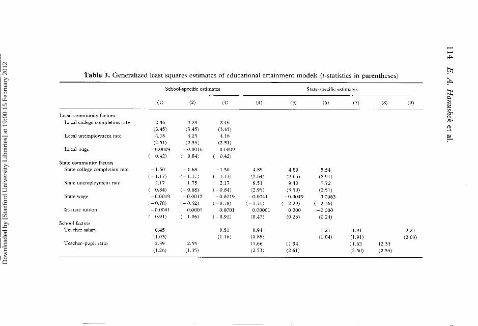
Table 3. Generalized least squares estimates of educational attainment models (t-statistics in parentheses)

School-specific estimates State-specific estimates

(1) (2) (3) (4) (5) (6) (7) (8) (9)

Local community factors Local college completion rate

Local unemployment rate

Local wage

State community factors State college completion rate

State unemployment rate

State wage

In-state tuition

School factors Teacher salary

Teacher-pupil ratio

Dow

nloa

ded

by [

Stan

ford

Uni

vers

ity L

ibra

ries

] at

19:

00 1

5 Fe

brua

ry 2

012

School Resource Efects 1 15

residuals from this auxiliary regression as the weight in the GLS estimation of equation (1 4).

The table in the appendix presents the coefficient estimates from the first stage regressions. As expected, academic attainment is positively related to the pretest score, parental education and family income. Whether school or state dummy variables are included appears to have little impact on the coefficient estimates. There are also significant between-school attainment differences. The hypotheses that the high-school dummy variables do not add to the explanatory power of the regressions can be rejected at any conventional level of significance.15

Basic Aggregation Effects

We turn now to the second stage regressions which contain information about the effects of school resources. Table 3 contains the results for the educational attainment specifications. The first three regressions use estimates of school value-added as the dependent variable; the remaining regressions use estimates of state value-added. The table reports the results of regressions which contain both the teacher-pupil ratio and teacher salary variables as well as regressions in which the two school characteristics are entered separately.

Consistent with most prior research, there is no evidence that either increasing the teacher-pupil ratio or raising teacher salaries increases student performance in any of the school-level regressions that are reported in Table 3. The coefficients for school resources are all insignificantly different from zero. Local community variations appear more important than state variations for educational attainment.

The state-level regressions reported in Table 3 vividly illustrate the potential for aggregation bias. Columns 4, 5 and 6 show that aggregation to the state level dramatically increases the coefficient estimates on both of the school characteristi- cs. Aggregation produces a significant coefficient on teacher-pupil ratio that is nearly five times as large in the aggregate as in the school specific regressions.

Moreover, as columns 7, 8 and 9 illustrate, excluding the partial set of community variables from the state-level regressions sharply increases the coeffi- cient and the statistical significance of the teacher salary variable. These results are broadly consistent with the notion that aggregating to the state level exacerbates the problem of omitted variable bias. Because aggregation tended to exacerbate the bias from excluding the observed community factors, it is also likely that aggrega- tion increased the bias due to the omission of other relevant factors.

Measurement Error

While the prior results are consistent with expectations about aggregate measure- ment error and omitted variables, they could also be consistent with a simple measurement error story for school-level resources. Aggregation moved the school resource and community environment coefficients away from zero, as would be predicted with classical measurement error. Thus the prior results do not conclus- ively demonstrate that aggregation-aggravated omitted variable bias is the sole problem.

A test of the competing hypotheses is based on traditional grouping methods applied so as to not confound grouping with possible omitted state or community factors.16 Grouping methods, which can be thought of as variants of instrumental variables, are based on aggregating observations within groups where group

Dow

nloa

ded

by [

Stan

ford

Uni

vers

ity L

ibra

ries

] at

19:

00 1

5 Fe

brua

ry 2

012

1 16 E. A. Hanushek et al.

Dow

nloa

ded

by [

Stan

ford

Uni

vers

ity L

ibra

ries

] at

19:

00 1

5 Fe

brua

ry 2

012

School Resource Efects 1 17

membership is determined by a variable that is correlated with the true explanatory variable but uncorrelated with the measurement error. Here, however, we add another component to creation of the groups because we also wish to find a grouping variable that is uncorrelated with omitted variables that also enter into the determination of school outcomes. Thus the choice of grouping variables, or instrumental variables, is more difficult than the standard situation where only measurement error is relevant.

The implicit use of state of residence as the grouping variable in the aggregate school resource studies likely violates the criterion that the grouping variable is uncorrelated with relevant omitted factors. Schools are not randomly sorted into states and a number of state policies such as those previously identified are likely to influence both achievement and school resource decisions. Therefore the finding that aggregation by state inflates coefficients does not by itself permit a distinction between omitted variables bias and measurement error explanations.

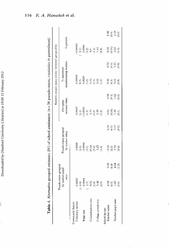
A way of distinguishing between the omitted variables and measurement error explanations is to regroup the schools into 'pseudo-states' which are correlated with the true school resources but not the omitted state policy factors. One plausible set of grouping variables simply uses the ordering of the school resources themselves- i.e. the ordering by the magnitude of the teacher-pupil ratio or the teacher salary.17 Grouping across teacher-pupil ratios will lead to consistent estimates if schools are correctly categorized on the basis of true (error-free) teacher-pupil ratios or true salaries, and there are no relevant omitted factors correlated with the true values of school resources. Because errors in measurement can lead to misclassification, an approach that balances efficiency and misclassification concerns is to omit observa- tions at the boundaries between groups, i.e. to produce trimmed group means. Here, we divide all schools into the 'state' groups and omit two schools at each group boundary, since these schools are the most likely to be wrongly classified.

A second approach orders states according to a state characteristic which is presumed to be correlated with school resource decisions but not directly corre- lated with achievement or with measurement errors. T o implement this, the states are first divided into four 'divisions' on the basis of the grouping variable. Within these divisions, schools are randomly assigned to pseudo-states. Schools in each pseudo-state share a similar division attribute, but the random assignment substan- tially weakens the link between schools and states.18 Because any single random allocation may give misleading point estimates, this random allocation of schools to pseudo-states is repeated 30 times for each state characteristic grouping variable, and the reported parameter estimates and standard errors are averages over the 30 replications.

Three state characteristics are used as instruments through creation of pseudo- divisions defined by rank ordering: (1) the state per-capita assessed property value; (2) the state poverty rate; and (3) the state percentage of workers unionized. The assumption is that controlling for observed family and community differences, each of these grouping variables will be correlated with true school resources but uncorrelated with both measurement error in the school resources and with any state- or local-specific omitted factors that explain student achievement. Of course, the last condition is difficult to verify and, indeed, is suspect when grouping is based on income or wealth-which might well be correlated with influences on school performance.

Each of these five grouping variables substantially weakens the link between schools and states. If aggregation by state leads to inflating school resource

Dow

nloa

ded

by [

Stan

ford

Uni

vers

ity L

ibra

ries

] at

19:

00 1

5 Fe

brua

ry 2

012

1 18 E. A. Hanushek et al.

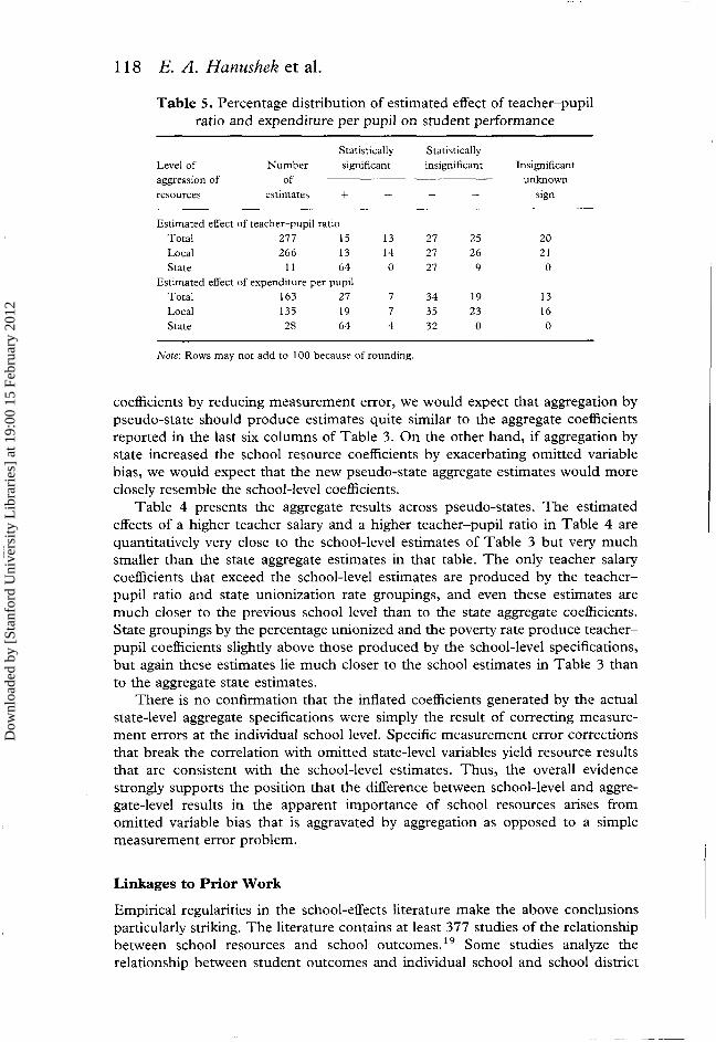
Table 5. Percentage distribution of estimated effect of teacher-pupil ratio and expenditure per pupil on student performance

Statistically Statistically Level of Number significant insignificant Insignificant aggression of of unknown resources estimates + - + - sign

Estimated effect of teacher-pupil ratio Total 277 15 13 27 25 20 Local 266 13 14 27 26 2 1 State 11 64 0 27 9 0

Estimated effect of expenditure per pupil Total 163 27 7 34 19 13 Local 135 19 7 35 23 16 State 28 64 4 32 0 0

Note: Rows may not add to 100 because of rounding.

coefficients by reducing measurement error, we would expect that aggregation by pseudo-state should produce estimates quite similar to the aggregate coefficients reported in the last six columns of Table 3. On the other hand, if aggregation by state increased the school resource coefficients by exacerbating omitted variable bias, we would expect that the new pseudo-state aggregate estimates would more closely resemble the school-level coefficients.

Table 4 presents the aggregate results across pseudo-states. The estimated effects of a higher teacher salary and a higher teacher-pupil ratio in Table 4 are quantitatively very close to the school-level estimates of Table 3 but very much smaller than the state aggregate estimates in that table. The only teacher salary coefficients that exceed the school-level estimates are produced by the teacher- pupil ratio and state unionization rate groupings, and even these estimates are much closer to the previous school level than to the state aggregate coefficients. State groupings by the percentage unionized and the poverty rate produce teacher- pupil coefficients slightly above those produced by the school-level specifications, but again these estimates lie much closer to the school estimates in Table 3 than to the aggregate state estimates.

There is no confirmation that the inflated coefficients generated by the actual state-level aggregate specifications were simply the result of correcting measure- ment errors at the individual school level. Specific measurement error corrections that break the correlation with omitted state-level variables yield resource results that are consistent with the school-level estimates. Thus, the overall evidence strongly supports the position that the difference between school-level and aggre- gate-level results in the apparent importance of school resources arises from omitted variable bias that is aggravated by aggregation as opposed to a simple measurement error problem.

Linkages to Prior Work

Empirical regularities in the school-effects literature make the above conclllsions particularly striking. The literature contains at least 377 studies of the relationship between school resources and school o ~ t c o m e s . ' ~ Some studies analyze the relationship between student outcomes and individual school and school district

Dow

nloa

ded

by [

Stan

ford

Uni

vers

ity L

ibra

ries

] at

19:

00 1

5 Fe

brua

ry 2

012

School Resource Eflects 1 19

Table 6. Percentage distribution of estimated effect of expenditure per pupil on student performance by outcome measure and aggregation of

resource effects

Measure of Statistically Statistically outcome and Number significant insignificant Insignificant, aggregation of of unknown resources estimates + - + - sign

Test score outcomes" Total 109 25 9 28 21 17 Local 101 2 1 9 30 23 18 State 8 75 13 13 0 0

Other (non-test) Outcomesh Total 54 3 1 2 46 15 6 Local 34 15 3 50 24 9 State 20 60 0 40 0 0

"All studies measure student performance by some form of standardized test score. hAll studies employ some outcome measure (such as income or school attainment) other than a standardized test score. Note: Rows may not add to 100 because of rounding.

characteristics while others use state average school characteristics. As Table 5 illustrates, the probability that a study reports a positive and statistically significant relationship between student achievement and school resources is much higher for the state-level analyses.

For example, consider the literature on teacher-pupil ratios and educational expenditures presented in Table 5. The first thing to note from the table is that the combined estimates from 277 separate investigations give no reason to believe that smaller classes are related to higher student p e r f ~ r m a n c e . ~ ~ The second thing to note is that the positive estimates (both statistically significant and total) come disproportionately from state-level analyses. While relatively few studies include state differences (1 I), almost two-thirds of these find positive and statistically significant effects of teacher-pupil ratios. When the resources are measured at the local level, any hint of disproportionate impact of smaller classes goes away. ('Local' implies measurement of school resources at the classroom, school or district level.)

Findings of positive expenditure effects also come disproportionately from analyses at the state level. Only 17% of the 163 estimates of school expenditure effects reported in Table 5 were conducted using state-level data on school characteristics. However, 42% of the estimates suggesting that higher spending is significantly associated with higher student performance come from these state- level studies. In contrast, the vast majority of studies at the local level do not support such a conclusion. '

Some previous speculation about why the production function results appear to differ from the results for earnings, specifically those of Card and Krueger (1992a,b), have centred on the measurement of outcomes. Table 6 divides the studies of expenditure effect into those using test scores to measure educational outcomes and those using any other outcome measures.22 Two-thirds of the studies consider test score measures with the remainder evaluating school attain- ment, drop-out behavior, earnings and other measures. This table makes it clear, however, that state-level analyses produce disproportionate numbers of estimates indicating that expenditure affects outcomes, regardless of how outcomes are

Dow

nloa

ded

by [

Stan

ford

Uni

vers

ity L

ibra

ries

] at

19:

00 1

5 Fe

brua

ry 2

012

120 E. A. Hanushek et al.

Table 7. Percentage distribution of estimated effect of teacher-pupil ratio and expenditure per pupil by state sampling scheme and aggregation

Statistically statistically significant insignificant Insignificant

State sampling scheme and Number of unknown aggregation of resource measures estimates + - + - sign

Teacher-pupil ratio Total 277 15 13 27 25 20 Single state samples" 157 12 18 31 31 8 Multiple state samplesh 120 18 8 21 18 3 5

With within-state variation' 109 14 8 20 19 39 Without within-state variation" 11 64 0 27 9 0

Expenditure per pupil Total 163 2 7 7 34 19 13 Single state samples" 89 20 11 30 26 12 Multiple state samplesh 74 3 5 1 39 11 14

With within-state variation' 46 17 0 43 18 22 Without within-state variation'' 28 64 4 32 0 0

"Estimates from samples drawn within single states. hEstimates from samples drawn across multiple states. 'Resource measures at level of classroom, school, district or county, allowing for variation within each state. "Resource measures aggregated to state level with no variation within each state Note: Rows may not add to 100 because of rounding

measured. Seventy-five per cent of the state-level estimates of expenditure on test performance and 60% of the state-level estimates of expenditure on non-test performance are positive and statistically significant, compared to at most 2 1% of the estimates of local expenditure.

The real key to understanding these results is found in Table 7 which focuses attention on the effects of omitted state policies. Studies aggregated to the state level necessarily draw samples across multiple states, such as in the Card and Krueger studies for national samples of workers. Studies with individual, school or district observations may or may not draw samples from multiple states. Samples drawn from entirely within an individual state contain schools all facing a common policy, so lack of measurement of important state policies will not bias the effects of variations in school resources. On the other hand, samples drawn across states without measurement of key policy differences will suffer from omitted variables bias. While the direction of bias is unknown a priori, Table 7 makes it clear that samples drawn across states are much more likely to point towards positive and statistically significant resource effects. Lower levels of data aggregation that preserve within-state variation in resources tend to have fewer findings of positive and statistically significant effects than with state aggregates, but they are much more heavily weighted to positive than to negative effects than the studies within individual states. In other words, the results of previous analyses support the pattern sketched in this paper: specification biases, present whenever samples cross state boundaries but fail to capture differences in state policies, are worsened by aggregation. Indeed, this simple story provides a reconciliation of the results of Card and Krueger (1 992a,b) with those of the previous education production functions-omissions of key state factors makes variations in school resources appear important while the better-specified, direct analyses of schools avoid such omitted variables biases.

Dow

nloa

ded

by [

Stan

ford

Uni

vers

ity L

ibra

ries

] at

19:

00 1

5 Fe

brua

ry 2

012

School Resource Eflects 12 1

Conclusions

A simple model of the relationship between aggregation and omitted variables bias demonstrates that aggregation to the state level increases the bias when the omitted variables are determined at the state level. A wide range of potentially relevant state policies, generally excluded because of data limitations, are likely to influence both school outcomes and school inputs positively. Under such conditions, the model suggests that aggregation to the state level inflates the apparent impact of school resources. Our empirical analysis of the relationship between school inputs and student educational attainment finds just that-aggregation to the state level increases the coefficients on school input variables. The pattern of results supports the hypothesis that aggregation increases omitted variable bias, but does not support the competing hypothesis that aggregation is beneficial because it reduces biases from measurement error.

This analysis provides a possible reconciliation of the apparently conflicting findings of wage studies and education production functions. A number of wage studies (see Card & IG-ueger, 1994; Betts, 1996) relate aggregate data on school resources to subsequent labor market success. These studies tend to find variations in school inputs such as class size or teacher salaries to be directly related to subsequent student outcomes. On the other hand, education production function studies (see Hanushek, 1986, 1989) have found little systematic relationship between disaggregated measures of school resources and more immediate student outcomes. While a variety of differences exist between the two types of studies, the analysis here focuses attention on the level of aggregation of the school resource measures and the consistent absence of measures of policy differences across states. The differences in results across the two types of studies are very consistent with the bias-enhancing effects of aggregation of misspecified relationships. With aggre- gate data, it is very difficult to identify the effects of school resources as distinct from unmeasured state policies.

These results provide additional evidence against the view that added expendi- tures alone are likely to improve student outcomes (see Hanushek et al., 1994).

Notes

1. Betts (1995) examines specific aspects of the Card and IG-rieger hetHodology in order to understand why their findings contradict much of the previous literature. pee also Heckman et al. (1996) and Speakrnan and Welch (1995) for an examination of the sensitivity of the estimates to the assumptions, the sample and the specification.

2. While the Card and IG-ueger studies have recently received attention, the literature goes back to Welch (1966) and Johnson and Stafford (1973). See Betts (1996).

3. There is considerable variation among the states in the rules regarding compulsory attend- ance. In 1992, most states allowed students to leave school at age 16, but eight states required students to attend school until age 17 and ten states required students to attend school until age 18 (US Department of Education, 1993). Similarly, the age at which students were required to start school ranged from 5 years old in Arkansas, Delaware and South Carolina to 8 years old in Arizona, Pennsylvania and Washington. On average, students were required to attend 10 years of primary and secondary schooling, but students in Arizona were only required to attend for 8 years, while students in Arkansas and Virginia were required to attend for 13 years.

4. The central concern is correlation of unmeasured determinants of student performance and measured school characteristics. Some attempts to analyze simultaneous policy decisions directly, albeit not in the form of value-added models, have emphasized its importance on the estimates (e.g. Brown & Saks, 1983; Akerhielm, 1955). For our empirical work, we are

Dow

nloa

ded

by [

Stan

ford

Uni

vers

ity L

ibra

ries

] at

19:

00 1

5 Fe

brua

ry 2

012

122 E. A. Hanushek et al.

interested in effects on school attainment over and above any achievement effects. It is natural to believe that any compensatory approaches and the induced simultaneity would have their primary impact on measured achievement.

5. For example, both Summers and Wolfe (1977) and Ferguson (1992) suggest significant non-linearities in the effects of class size on student achievement. Summers and Wolfe further suggest that class size may have differential effects depending on the level of achievement of individual students. Bryk and Raudenbush (1992) examine a variety of specialized non-linear models in the context of schools. None of this analysis generalizes in any simple way to non-linear models.

6. Early discussion of aggregation is found in Theil (1971). The discussion of aggregation with model mispecification can be found in Grunfeld and Griliches (1960).

7. The omitted variable bias becomes much more complicated when multiple included and excluded variables are considered, and the effects of aggregation can no longer in general be ascertained.

8. State mean expenditure levels reflect both local and state expenditures. Therefore, within- state variation results both from differences in local values of A and the method by which states allocate money to districts.

9. Card and Krueger (1994) highlight fluctuations in capital expenditure or inexplicable annual movements in pupil-teacher ratios as evidence of this sort of error. While annual movements in pupil-teacher ratios or other inputs have little impact on value-added models, they will obviously introduce serious measurement errors in the cumulative inputs.

10. In this simple case of measurement error, the error is assumed independent of the included variables. Systematic measurement error will not have such clear effects.

11. The measurement error model does not yield any simple predictions when more than one variable is measured with error (see, for example, Maddala, 1977, p. 294). With multiple measurement errors, the coefficients are not necessarily biased towards zero, but instead depend on the entire pattern of covariance among the exogenous variables.

12. In Hanushek et al. (1996), we also analyze achievement differences in the context of a more complicated model structure. The achievement analysis employs a different HSB cohort made up of students who were sophomores in 1980.

13. Approximately 20% of individuals are still in school and recent trends suggest many non-students will return to school at some point in the future. Thus, we are not measuring years of schoolingultimately completed. Students might complete a degree associated with 8 years of post-secondary schooling in fewer than 8 calendar years, leading to the coding employed.

14. HSB survey contains very little information on community environment, leading us to use US census data to construct measures of local unemployment, wage and college completion rates. Rivkin (1991) describes the construction of the community characteristics. As a general rule, our measures of state community characteristics are aggregated from our measures of local community characteristics. The information on university tuition is taken from Peterson's Guide to Four Year Colleges (1984).

15. The F-test statistic equals 2.32 (306, 1993 degrees of freedom) for the post-secondary schooling regression.

16. Similar approach of looking for between-jurisdiction differences has been independently proposed in Heckman (1994). His discussion provides a public choice rationale for the - -

existence of such differences. 17. Early proposals for grouping and instrumental variables concentrated on bivariate models and

analyzed the trade-off between bias and efficiency from aggregating to two groups (Wald), three with an omitted center category (Bartlett), and multiple groups (Durbin) (see Maddala, 1977, pp. 296-300; Pakes, 1982). The approach here is an extension of these. For a general consideration of instrumental variables in cross-sections, see White (1982).

18. A completely random assignment of schools to pseudo-states without first grouping by divisions based on some underlying factor would fully break the link between schools and states. However, this strategy would also eliminate all differences between pseudo-states in the expected values of the variables, thus making aggregate estimates meaningless.

19. For these purposes, a 'study' is a separate estiniate of an educational production function. An individual publication may include several studies, pertaining to different grade levels or measurement of outcomes. Alternative specifications of the same basic model were not double counted; nor was publication of the same basic results in different sources. The attempt was to record the information from all published studies that included one of the

Dow

nloa

ded

by [

Stan

ford

Uni

vers

ity L

ibra

ries

] at

19:

00 1

5 Fe

brua

ry 2

012

School Resource Efects 123

central measures of resources (either of real resources of pupil-teacher ratios, teacher experience, teacher education, facilities, or administrator characteristics or monetary re- sources of expenditures per student or salaries), recorded information about the statistical significance of the estimated relationships, and included some measure of family and non-school inputs. Hanushek's (1989) summary missed a few estimates that were available prior to mid-1988, and these have been incorporated in the update through 1994. The best way to tabulate the results across different studies has been the subject of lively debate (see Hedges et al., 1994; Hanushek, 1994). The issues raised in that debate, however, are generally not relevant for the issues of aggregation considered here.

20. Not all studies contained information on each specific resource. Of the 377 studies looking at any of the identified resources, 277 analyzed either teacher-pupil ratios, pupil-teacher ratios or class size. (All analyses of pupil-teacher ratios are put in terms of teacher-pupil ratios by reversing the signs.)

21. The separate analysis of resource effects by Hedges et al. (1994) concentrates on expenditure studies without regard to the quality of the underlying analysis.

22. See Betts (1996) for further discussion of aggregation patterns among studies in which earnings are used to measure achievement.

References

Aitken, M. & Longford, N. (1986) Statistical modelling issues in school effectiveness studies, Journal of the Royal Statistical Society, Series A, 149, pp. 1-26.

Betts, J. R. (1995) Does school quality matter? Evidence from the National Longitudinal Survey of Youth, Review of Economics and Statistics, 77, pp. 231-247.

Betts, J. R. (1996) Is there a link between school inputs and earnings? Fresh scrutiny of an old literature, in: Burtless, G. (Ed.) Does Money Matter? The Effect of School Resources on Student Achievement and Adult Success (Washington, DC, Brookings), pp. 141-191.

Bishop, J. (1992) The impact of academic competencies of wages, unemployment, and job performance, Carnegie-Rochester Conference Series on Public Policy, 37, pp. 127-194.

Borjas, G. (1987) Self-selection and the earnings of immigrants, American Economic Review, 77, pp. 531-553.

Bryk, A. S. & Raudenbush, S. W. (1992) Hierarchical Linear Models: Applications and Data Analysis Methods (Newbury Park, CA, Sage).

Burtless, G. (Ed.) (1996) Does Money Matter? The Effect of School Resources on Student Achievement and Adult Success (Washington, DC, Brookings).

Card, D. & I h e g e r , A. B. (1992a) Does school quality matter? Returns to education and the characreristics of pubic schools in the United States, Journal of Political Economy, 100, pp. 1-40.

Card, D. & Krueger, A. B. (1992b) School quality and black-white relative earnings: a direct assessment, Quarterly Journal of Economics, 107, pp. 15 1-200. .

Card, D. & Krueger, A. B. (1994) The economic return to school quality: a partial survey, Industrial Relations Section, Princeton University, Working Paper 334, October.

Coleman, J. S., Campbell, E. Q., Hobson, C. J., McPartland, J., Mood, A. M., Weinfeld, F. D. & York, R. L. (1966) Equality of Educational Opportunity (Washington, DC, US Government Printing Office).

Ferguson, R. (1991) Paying for public education: new evidence on how and why money matters, Harvard Journal on Legislation, 28, pp. 465-498.

Gold, S. D., Smith, D. M., Lawton, S. B. & Hyary, A. (1991) Public School Finance Programs of the United States and Canada: 1900-91 (New York, The Nelson A. Rockefeller Institute of Government, State University of New York).

Grunfeld, Y. & Griliches, Z. (1960) Is aggregation necessarily bad?, Review of Economics and Statistics, 62, pp. 1-13.

Hanushek, E. A. (1974) Efficient estimators for regressing regression coefficients, The American Statistician, 28, pp. 66-67.

Hanushek, E. A. (1979) Conceptual and empirical issues in the estimation of educational production functions, Journal of Human Resources, 14, pp. 351-388.

Hanushek, E. A. (1986) The economics of schooling: production and efficiency in public schools, Journal of Economic Literature, 24, pp. 1 141-1 177.

Hanushek, E. A. (1989) The impact of differential expenditures on school performance, Educational Researcher, 18, pp. 45-51.

Dow

nloa

ded

by [

Stan

ford

Uni

vers

ity L

ibra

ries

] at

19:

00 1

5 Fe

brua

ry 2

012

124 E. A. Hanushek et al.

Hanushek, E. A. (1994) Money might matter somewhere: a response to Hedges, Laine, and Greenwald, Educational Researcher, 23, pp. 5-8.

Hanushek, E. A. (1996) Assessing the effects of school resources on student performance: an update, Rochester Center for Economics Research, Working Paper 424.

Hanushek, E. A. & Rivkin, S. G. (1997) Understanding the 20th century explosion in US school costs, Journal of Human Resources (in press).

Hanushek, E. A. & Taylor, L. L. (1990) Alternative assessments of the performance of schools: measurement of state variations in achievement, Journal of Humaiz Resources, 25, pp. 179-201.

Hanushek, E. A. et al. (1994) Making Schools Work: Iwlprovivzg Perjormance and Controlling Costs (Washington, DC, Brookings Institution).

Hanushek, E. A,, Rivkin, S. G. & Taylor, L. L. (1996) Aggregation and the estimated effects of school resources, Review of Ecov~omics and Statistics (in press).

Heckrnan, J. J. (1994) Aggregation bias and schooling quality, University of Chicago, December, mimeo.

Heckman, J. J., Layne-Farrar, A. S. & Todd, P. E. (1996) Does measured school quality really matter? An examination of the earnings-quality relationship, in: Burtless, G. (Ed.) Does Money Matter? The Effect of School Resources on Student Achievenzent aizd Adult Success (Washington, DC, Brookings), pp. 192-289.

Hedges, L. V., Laine, R. D. & Greenwald, R. (1994) Does money matter? A meta-analysis of studies of the effects of differential school inputs on student outcomes, Educational Researcher, 23, pp. 5-14.

Johnson, G. E. & Stafford, F. P. (1973) Social returns to quantity and quality of schooling, Journal of Human Resources, 8, pp. 139-155.

Maddala, G. S. (1977) Econometrics (New York, McGraw-Hill). Mayston, D. J. (1996) Educational attainment and resource use: mystery or econometric

misspecification, Education Economics, 4, pp. 127-1 42. Pakes, A. (1982) On the asymptotic bias of Wald-type estimators of a straight-line when both

variables are subject to error, International Econonzic Review, 23, pp. 491-497. Peterson's Guide to Four Year Colleges (1982) (Princeton, NJ, Peterson's Guide). Rivkin, S. G. (1991) Schooling and employment in the 1980s: who succeeds?, PhD Dissertation,

University of California, Los Angeles. Rivkin, S. E. (1993) School desegregation, academic attainment and employment, Department

of Economics, Amherst College, mimeo. Speakman, R. & Welch, F. (1995) Does school quality matter?-A reassessment, Texas A&M

University, January, mimeo. Summers, A. & Wolfe, B. (1977) Do schools make a difference?, American Economic Review, 67,

pp. 639-652. Swamy, P. A. V. B. (1970) Efficient inference in a random coefficient regression model,

Econometrica, 38, pp. 3 1 1-323. Theil, H. (1971) Principles of Econon~etncs (New York, John Wiley & Sons). Tiebout, C. M. (1956) A pure theory of local expenditures, Journal of Political Econorny, 64, pp.

4 16-424. US Bureau of The Census (1992) Statistical Abstract of the United States (Washington, DC, US

Government Printing Office). US Department of Education (1993) The Condition of Education 1993 (Washington, DC,

Education, National Center for Education Statistics). Welch, F. (1966) Measurement of the quality of schooling, American Ecoizonlic Review, 56, pp.

379-392. White, H. (1982) Instrumental variables regression with independent observations, Econometrica,

50, pp. 483-499.

Dow

nloa

ded

by [

Stan

ford

Uni

vers

ity L

ibra

ries

] at

19:

00 1

5 Fe

brua

ry 2

012

School Resource Efects 125

Appendix: Within-group Parameter Estimates for Test Score Production and School Attainment (t-statistics

in parentheses)

Years of schooling completed

School fixed State fixed Variable effects effects

12th Grade test score 0.17 0.16 (19.8) (20.8)

Father's education 0.10 0.11 (6.16) (7.06)

Father's education unknown 1.14 1.18 (4.50) (4.94)

Mother's education 0.1 1 0.11 (5.40) (6.12)

Mother's education unknown 1.16 1.08 (2.87) (2.84)

Family income US812 000-20 000 - 0.08 -0.12 (-0.88) (- 1.40)

Family income over US$20 000 0.28 0.27 (2.82) (2.88)

Female 0.16 0.16 (2.42) (2.69)

Black 0.39 0.47 (3.46) (5.57)

Total observations 2309 2309

Dow

nloa

ded

by [

Stan

ford

Uni

vers

ity L

ibra

ries

] at

19:

00 1

5 Fe

brua

ry 2

012

Dow

nloa

ded

by [

Stan

ford

Uni

vers

ity L

ibra

ries

] at

19:

00 1

5 Fe

brua

ry 2

012