the idea of the fundamental group - cornell universitymath.cornell.edu/~hatcher/at/atch1.pdfthe idea...
TRANSCRIPT

Algebraic topology can be roughly defined as the study of techniques for forming
algebraic images of topological spaces. Most often these algebraic images are groups,
but more elaborate structures such as rings, modules, and algebras also arise. The
mechanisms that create these images — the ‘lanterns’ of algebraic topology, one might
say — are known formally as functors and have the characteristic feature that they
form images not only of spaces but also of maps. Thus, continuous maps between
spaces are projected onto homomorphisms between their algebraic images, so topo-
logically related spaces have algebraically related images.
With suitably constructed lanterns one might hope to be able to form images with
enough detail to reconstruct accurately the shapes of all spaces, or at least of large
and interesting classes of spaces. This is one of the main goals of algebraic topology,
and to a surprising extent this goal is achieved. Of course, the lanterns necessary to
do this are somewhat complicated pieces of machinery. But this machinery also has
a certain intrinsic beauty.
This first chapter introduces one of the simplest and most important functors
of algebraic topology, the fundamental group, which creates an algebraic image of a
space from the loops in the space, the paths in the space starting and ending at the
same point.
The Idea of the Fundamental Group
To get a feeling for what the fundamental group is about, let us look at a few
preliminary examples before giving the formal definitions.
22 Chapter 1 The Fundamental Group
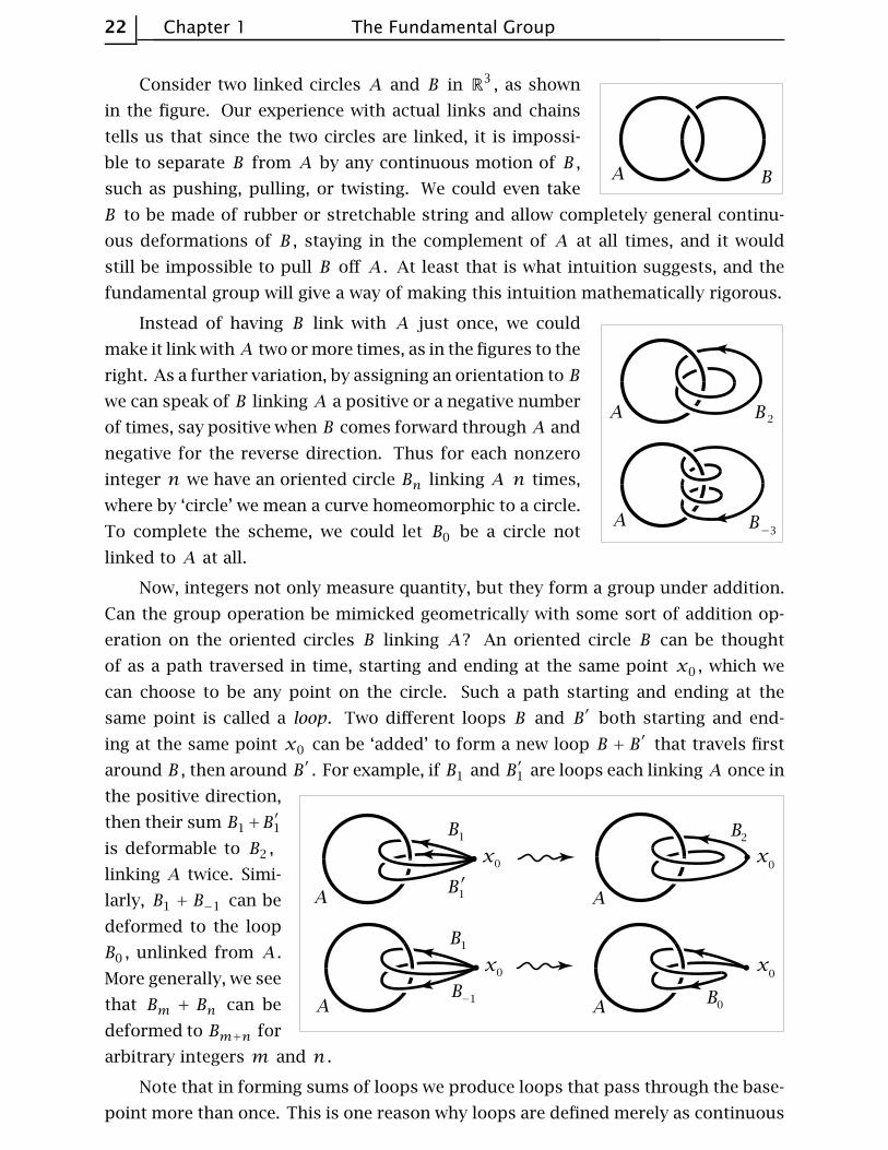
Consider two linked circles A and B in R3 , as shown
in the figure. Our experience with actual links and chains
tells us that since the two circles are linked, it is impossi-
ble to separate B from A by any continuous motion of B ,
such as pushing, pulling, or twisting. We could even take
B to be made of rubber or stretchable string and allow completely general continu-
ous deformations of B , staying in the complement of A at all times, and it would
still be impossible to pull B off A . At least that is what intuition suggests, and the
fundamental group will give a way of making this intuition mathematically rigorous.
Instead of having B link with A just once, we could
make it link with A two or more times, as in the figures to the
right. As a further variation, by assigning an orientation to B
we can speak of B linking A a positive or a negative number
of times, say positive when B comes forward through A and
negative for the reverse direction. Thus for each nonzero
integer n we have an oriented circle Bn linking A n times,
where by ‘circle’ we mean a curve homeomorphic to a circle.
To complete the scheme, we could let B0 be a circle not
linked to A at all.
Now, integers not only measure quantity, but they form a group under addition.
Can the group operation be mimicked geometrically with some sort of addition op-
eration on the oriented circles B linking A? An oriented circle B can be thought
of as a path traversed in time, starting and ending at the same point x0 , which we
can choose to be any point on the circle. Such a path starting and ending at the
same point is called a loop. Two different loops B and B′ both starting and end-
ing at the same point x0 can be ‘added’ to form a new loop B + B′ that travels first
around B , then around B′ . For example, if B1 and B′1 are loops each linking A once in
the positive direction,
then their sum B1+B′1
is deformable to B2 ,
linking A twice. Simi-
larly, B1 + B−1 can be
deformed to the loop
B0 , unlinked from A .
More generally, we see
that Bm + Bn can be
deformed to Bm+n for
arbitrary integers m and n .
Note that in forming sums of loops we produce loops that pass through the base-
point more than once. This is one reason why loops are defined merely as continuous

The Idea of the Fundamental Group 23
paths, which are allowed to pass through the same point many times. So if one is
thinking of a loop as something made of stretchable string, one has to give the string
the magical power of being able to pass through itself unharmed. However, we must
be sure not to allow our loops to intersect the fixed circle A at any time, otherwise we
could always unlink them from A .
Next we consider a slightly more complicated sort of linking, involving three cir-
cles forming a configuration known as the Borromean rings, shown at the left in the fig-
ure below. The interesting feature here is that if any one of the three circles is removed,
the other two are not
linked. In the same
spirit as before, let us
regard one of the cir-
cles, say C , as a loop
in the complement of
the other two, A and
B , and we ask whether C can be continuously deformed to unlink it completely from
A and B , always staying in the complement of A and B during the deformation. We
can redraw the picture by pulling A and B apart, dragging C along, and then we see
C winding back and forth between A and B as shown in the second figure above.
In this new position, if we start at the point of C indicated by the dot and proceed
in the direction given by the arrow, then we pass in sequence: (1) forward through
A , (2) forward through B , (3) backward through A , and (4) backward through B . If
we measure the linking of C with A and B by two integers, then the ‘forwards’ and
‘backwards’ cancel and both integers are zero. This reflects the fact that C is not
linked with A or B individually.
To get a more accurate measure of how C links with A and B together, we re-
gard the four parts (1)–(4) of C as an ordered sequence. Taking into account the
directions in which these segments of C pass
through A and B , we may deform C to the sum
a+b−a−b of four loops as in the figure. We
write the third and fourth loops as the nega-
tives of the first two since they can be deformed
to the first two, but with the opposite orienta-
tions, and as we saw in the preceding exam-
ple, the sum of two oppositely oriented loops
is deformable to a trivial loop, not linked with
anything. We would like to view the expression
a + b − a − b as lying in a nonabelian group, so that it is not automatically zero.
Changing to the more usual multiplicative notation for nonabelian groups, it would
be written aba−1b−1 , the commutator of a and b .
24 Chapter 1 The Fundamental Group
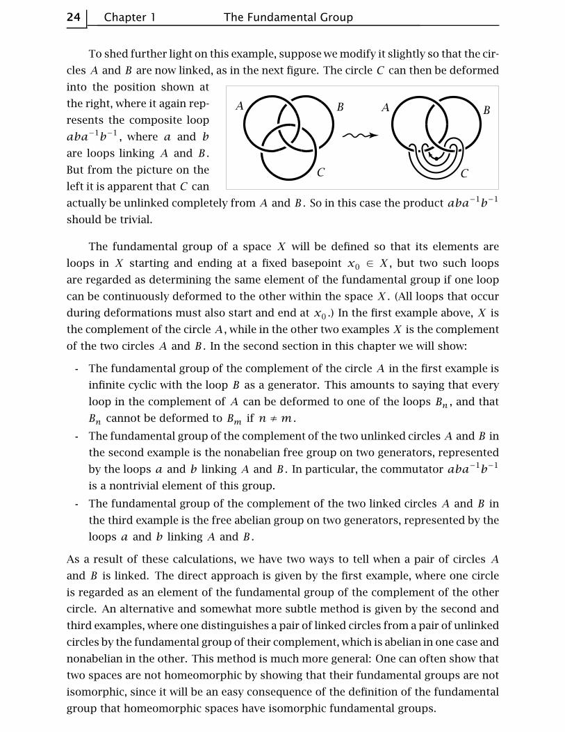
To shed further light on this example, suppose we modify it slightly so that the cir-
cles A and B are now linked, as in the next figure. The circle C can then be deformed
into the position shown at
the right, where it again rep-
resents the composite loop
aba−1b−1 , where a and b
are loops linking A and B .
But from the picture on the
left it is apparent that C can
actually be unlinked completely from A and B . So in this case the product aba−1b−1
should be trivial.
The fundamental group of a space X will be defined so that its elements are
loops in X starting and ending at a fixed basepoint x0 ∈ X , but two such loops
are regarded as determining the same element of the fundamental group if one loop
can be continuously deformed to the other within the space X . (All loops that occur
during deformations must also start and end at x0 .) In the first example above, X is
the complement of the circle A , while in the other two examples X is the complement
of the two circles A and B . In the second section in this chapter we will show:
The fundamental group of the complement of the circle A in the first example is
infinite cyclic with the loop B as a generator. This amounts to saying that every
loop in the complement of A can be deformed to one of the loops Bn , and that
Bn cannot be deformed to Bm if n ≠m .
The fundamental group of the complement of the two unlinked circles A and B in
the second example is the nonabelian free group on two generators, represented
by the loops a and b linking A and B . In particular, the commutator aba−1b−1
is a nontrivial element of this group.
The fundamental group of the complement of the two linked circles A and B in
the third example is the free abelian group on two generators, represented by the
loops a and b linking A and B .
As a result of these calculations, we have two ways to tell when a pair of circles A
and B is linked. The direct approach is given by the first example, where one circle
is regarded as an element of the fundamental group of the complement of the other
circle. An alternative and somewhat more subtle method is given by the second and
third examples, where one distinguishes a pair of linked circles from a pair of unlinked
circles by the fundamental group of their complement, which is abelian in one case and
nonabelian in the other. This method is much more general: One can often show that
two spaces are not homeomorphic by showing that their fundamental groups are not
isomorphic, since it will be an easy consequence of the definition of the fundamental
group that homeomorphic spaces have isomorphic fundamental groups.

Basic Constructions Section 1.1 25
This first section begins with the basic definitions and constructions, and then
proceeds quickly to an important calculation, the fundamental group of the circle,
using notions developed more fully in §1.3. More systematic methods of calculation
are given in §1.2. These are sufficient to show for example that every group is realized
as the fundamental group of some space. This idea is exploited in the Additional
Topics at the end of the chapter, which give some illustrations of how algebraic facts
about groups can be derived topologically, such as the fact that every subgroup of a
free group is free.
Paths and Homotopy
The fundamental group will be defined in terms of loops and deformations of
loops. Sometimes it will be useful to consider more generally paths and their defor-
mations, so we begin with this slight extra generality.
By a path in a space X we mean a continuous map f : I→X where I is the unit
interval [0,1] . The idea of continuously deforming a path, keeping its endpoints
fixed, is made precise by the following definition. A homotopy of paths in X is a
family ft : I→X , 0 ≤ t ≤ 1, such that
(1) The endpoints ft(0) = x0 and ft(1) = x1
are independent of t .
(2) The associated map F : I×I→X defined by
F(s, t) = ft(s) is continuous.
When two paths f0 and f1 are connected in this way by a homotopy ft , they are said
to be homotopic. The notation for this is f0 ≃ f1 .
Example 1.1: Linear Homotopies. Any two paths f0 and f1 in Rn having the same
endpoints x0 and x1 are homotopic via the homotopy ft(s) = (1− t)f0(s)+ tf1(s) .
During this homotopy each point f0(s) travels along the line segment to f1(s) at con-
stant speed. This is because the line through f0(s) and f1(s) is linearly parametrized
as f0(s) + t[f1(s) − f0(s)] = (1 − t)f0(s) + tf1(s) , with the segment from f0(s) to
f1(s) covered by t values in the interval from 0 to 1. If f1(s) happens to equal f0(s)
then this segment degenerates to a point and ft(s) = f0(s) for all t . This occurs in
particular for s = 0 and s = 1, so each ft is a path from x0 to x1 . Continuity of
the homotopy ft as a map I×I→Rn follows from continuity of f0 and f1 since the
algebraic operations of vector addition and scalar multiplication in the formula for ftare continuous.
This construction shows more generally that for a convex subspace X ⊂ Rn , all
paths in X with given endpoints x0 and x1 are homotopic, since if f0 and f1 lie in
X then so does the homotopy ft .
26 Chapter 1 The Fundamental Group
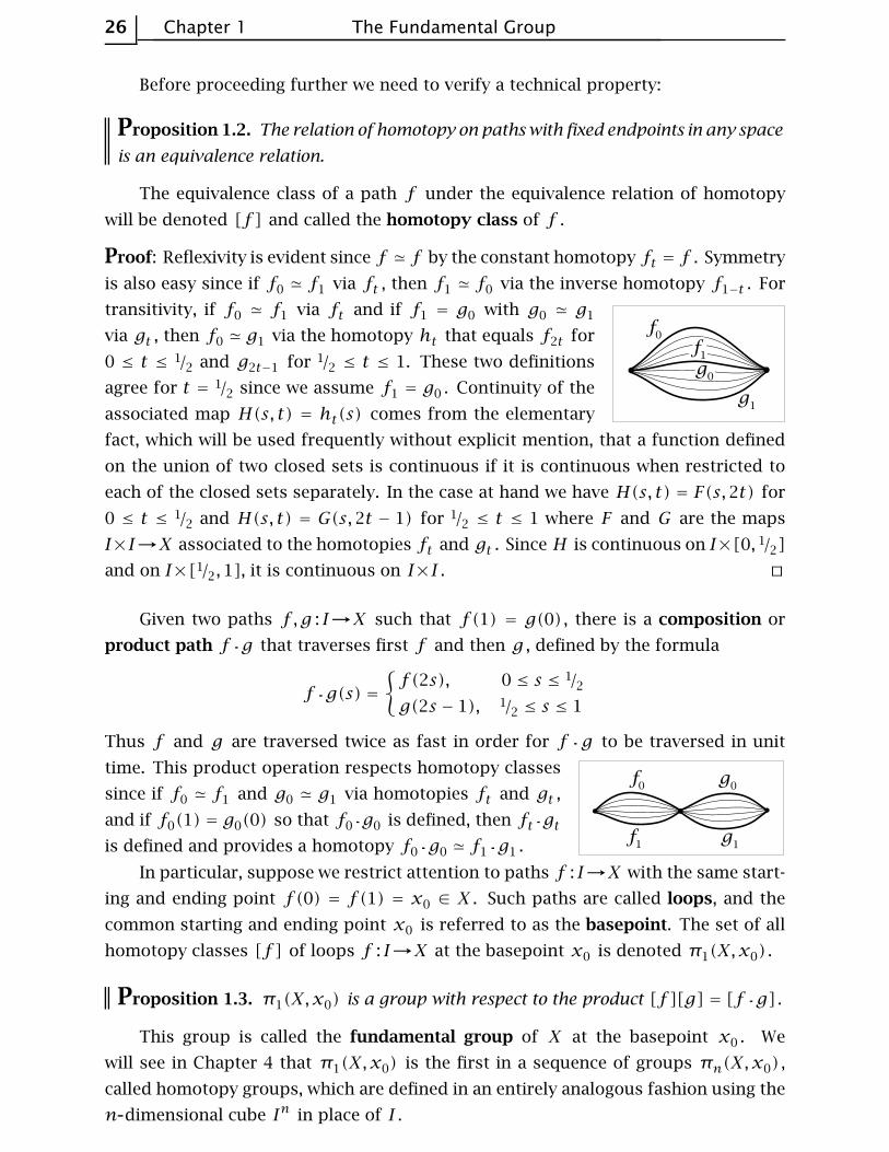
Before proceeding further we need to verify a technical property:
Proposition 1.2. The relation of homotopy on paths with fixed endpoints in any space
is an equivalence relation.
The equivalence class of a path f under the equivalence relation of homotopy
will be denoted [f ] and called the homotopy class of f .
Proof: Reflexivity is evident since f ≃ f by the constant homotopy ft = f . Symmetry
is also easy since if f0 ≃ f1 via ft , then f1 ≃ f0 via the inverse homotopy f1−t . For
transitivity, if f0 ≃ f1 via ft and if f1 = g0 with g0 ≃ g1
via gt , then f0 ≃ g1 via the homotopy ht that equals f2t for
0 ≤ t ≤ 1/2 and g2t−1 for 1/2 ≤ t ≤ 1. These two definitions
agree for t = 1/2 since we assume f1 = g0 . Continuity of the
associated map H(s, t) = ht(s) comes from the elementary
fact, which will be used frequently without explicit mention, that a function defined
on the union of two closed sets is continuous if it is continuous when restricted to
each of the closed sets separately. In the case at hand we have H(s, t) = F(s,2t) for
0 ≤ t ≤ 1/2 and H(s, t) = G(s,2t − 1) for 1/2 ≤ t ≤ 1 where F and G are the maps
I×I→X associated to the homotopies ft and gt . Since H is continuous on I×[0, 1/2]
and on I×[1/2,1], it is continuous on I×I . ⊔⊓
Given two paths f ,g : I→X such that f(1) = g(0) , there is a composition or
product path f g that traverses first f and then g , defined by the formula
f g(s) =
{f(2s), 0 ≤ s ≤ 1/2g(2s − 1), 1/2 ≤ s ≤ 1
Thus f and g are traversed twice as fast in order for f g to be traversed in unit
time. This product operation respects homotopy classes
since if f0 ≃ f1 and g0 ≃ g1 via homotopies ft and gt ,
and if f0(1) = g0(0) so that f0 g0 is defined, then ft gtis defined and provides a homotopy f0 g0 ≃ f1 g1 .
In particular, suppose we restrict attention to paths f : I→X with the same start-
ing and ending point f(0) = f(1) = x0 ∈ X . Such paths are called loops, and the
common starting and ending point x0 is referred to as the basepoint. The set of all
homotopy classes [f ] of loops f : I→X at the basepoint x0 is denoted π1(X,x0) .
Proposition 1.3. π1(X,x0) is a group with respect to the product [f ][g] = [f g] .
This group is called the fundamental group of X at the basepoint x0 . We
will see in Chapter 4 that π1(X,x0) is the first in a sequence of groups πn(X,x0) ,
called homotopy groups, which are defined in an entirely analogous fashion using the
n dimensional cube In in place of I .
Basic Constructions Section 1.1 27
Proof: By restricting attention to loops with a fixed basepoint x0 ∈ X we guarantee
that the product f g of any two such loops is defined. We have already observed
that the homotopy class of f g depends only on the homotopy classes of f and g ,
so the product [f ][g] = [f g] is well-defined. It remains to verify the three axioms
for a group.
As a preliminary step, define a reparametrization of a path f to be a composi-
tion fϕ where ϕ : I→I is any continuous map such that ϕ(0) = 0 and ϕ(1) = 1.
Reparametrizing a path preserves its homotopy class since fϕ ≃ f via the homotopy
fϕt where ϕt(s) = (1 − t)ϕ(s) + ts so that ϕ0 = ϕ and ϕ1(s) = s . Note that
(1 − t)ϕ(s) + ts lies between ϕ(s) and s , hence is in I , so the composition fϕt is
defined.
If we are given paths f ,g,h with f(1) = g(0) and g(1) = h(0) , then both prod-
ucts (f g)h and f (g h) are defined, and f (g h) is a reparametrization
of (f g) h by the piecewise linear function ϕ whose graph is shown
in the figure at the right. Hence (f g) h ≃ f (g h) . Restricting atten-
tion to loops at the basepoint x0 , this says the product in π1(X,x0) is
associative.
Given a path f : I→X , let c be the constant path at f(1) , defined by c(s) = f(1)
for all s ∈ I . Then f c is a reparametrization of f via the function ϕ whose graph is
shown in the first figure at the right, so f c ≃ f . Similarly,
c f ≃ f where c is now the constant path at f(0) , using
the reparametrization function in the second figure. Taking
f to be a loop, we deduce that the homotopy class of the
constant path at x0 is a two-sided identity in π1(X,x0) .
For a path f from x0 to x1 , the inverse path f from x1 back to x0 is defined
by f(s) = f(1 − s) . To see that f f is homotopic to a constant path we use the
homotopy ht = ft gt where ft is the path that equals f on the interval [0,1 − t]
and that is stationary at f(1− t) on the interval [1− t,1] , and gt is the inverse path
of ft . We could also describe ht in terms of the associated function
H : I×I→X using the decomposition of I×I shown in the figure. On
the bottom edge of the square H is given by f f and below the ‘V’ we
let H(s, t) be independent of t , while above the ‘V’ we let H(s, t) be
independent of s . Going back to the first description of ht , we see that since f0 = f
and f1 is the constant path c at x0 , ht is a homotopy from f f to c c = c . Replacing
f by f gives f f ≃ c for c the constant path at x1 . Taking f to be a loop at the
basepoint x0 , we deduce that [f ] is a two-sided inverse for [f ] in π1(X,x0) . ⊔⊓
Example 1.4. For a convex set X in Rn with basepoint x0 ∈ X we have π1(X,x0) = 0,
the trivial group, since any two loops f0 and f1 based at x0 are homotopic via the
linear homotopy ft(s) = (1− t)f0(s)+ tf1(s) , as described in Example 1.1.
28 Chapter 1 The Fundamental Group
It is not so easy to show that a space has a nontrivial fundamental group since one
must somehow demonstrate the nonexistence of homotopies between certain loops.
We will tackle the simplest example shortly, computing the fundamental group of the
circle.
It is natural to ask about the dependence of π1(X,x0) on the choice of the base-
point x0 . Since π1(X,x0) involves only the path-component of X containing x0 , it
is clear that we can hope to find a relation between π1(X,x0) and π1(X,x1) for two
basepoints x0 and x1 only if x0 and x1 lie in the same path-component of X . So
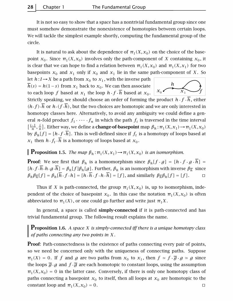
let h : I→X be a path from x0 to x1 , with the inverse path
h(s) = h(1−s) from x1 back to x0 . We can then associate
to each loop f based at x1 the loop h f h based at x0 .
Strictly speaking, we should choose an order of forming the product h f h , either
(h f) h or h (f h) , but the two choices are homotopic and we are only interested in
homotopy classes here. Alternatively, to avoid any ambiguity we could define a gen-
eral n fold product f1 ··· fn in which the path fi is traversed in the time interval[ i−1n ,
in
]. Either way, we define a change-of-basepoint map βh :π1(X,x1)→π1(X,x0)
by βh[f ] = [h f h] . This is well-defined since if ft is a homotopy of loops based at
x1 then h ft h is a homotopy of loops based at x0 .
Proposition 1.5. The map βh :π1(X,x1)→π1(X,x0) is an isomorphism.
Proof: We see first that βh is a homomorphism since βh[f g] = [h f g h] =
[h f h h g h] = βh[f ]βh[g] . Further, βh is an isomorphism with inverse βh since
βhβh[f ] = βh[h f h] = [h h f h h] = [f ] , and similarly βhβh[f ] = [f ] . ⊔⊓
Thus if X is path-connected, the group π1(X,x0) is, up to isomorphism, inde-
pendent of the choice of basepoint x0 . In this case the notation π1(X,x0) is often
abbreviated to π1(X) , or one could go further and write just π1X .
In general, a space is called simply-connected if it is path-connected and has
trivial fundamental group. The following result explains the name.
Proposition 1.6. A space X is simply-connected iff there is a unique homotopy class
of paths connecting any two points in X .
Proof: Path-connectedness is the existence of paths connecting every pair of points,
so we need be concerned only with the uniqueness of connecting paths. Suppose
π1(X) = 0. If f and g are two paths from x0 to x1 , then f ≃ f g g ≃ g since
the loops g g and f g are each homotopic to constant loops, using the assumption
π1(X,x0) = 0 in the latter case. Conversely, if there is only one homotopy class of
paths connecting a basepoint x0 to itself, then all loops at x0 are homotopic to the
constant loop and π1(X,x0) = 0. ⊔⊓

Basic Constructions Section 1.1 29
The Fundamental Group of the Circle
Our first real theorem will be the calculation π1(S1) ≈ Z . Besides its intrinsic
interest, this basic result will have several immediate applications of some substance,
and it will be the starting point for many more calculations in the next section. It
should be no surprise then that the proof will involve some genuine work.
Theorem 1.7. π1(S1) is an infinite cyclic group generated by the homotopy class of
the loop ω(s) = (cos 2πs, sin 2πs) based at (1,0) .
Note that [ω]n = [ωn] where ωn(s) = (cos 2πns, sin 2πns) for n ∈ Z . The
theorem is therefore equivalent to the statement that every loop in S1 based at (1,0)
is homotopic to ωn for a unique n ∈ Z . To prove this the idea will
be to compare paths in S1 with paths in R via the map p :R→S1
given by p(s) = (cos 2πs, sin 2πs) . This map can be visualized
geometrically by embedding R in R3 as the helix parametrized by
s֏ (cos 2πs, sin 2πs, s) , and then p is the restriction to the helix
of the projection of R3 onto R2 , (x,y, z)֏ (x,y) . Observe that
the loop ωn is the composition pωn where ωn : I→R is the path
ωn(s) = ns , starting at 0 and ending at n , winding around the helix
|n| times, upward if n > 0 and downward if n < 0. The relation
ωn = pωn is expressed by saying that ωn is a lift of ωn .
We will prove the theorem by studying how paths in S1 lift to paths in R . Most
of the arguments will apply in much greater generality, and it is both more efficient
and more enlightening to give them in the general context. The first step will be to
define this context.
Given a space X , a covering space of X consists of a space X and a map p : X→Xsatisfying the following condition:
(∗)
For each point x ∈ X there is an open neighborhood U of x in X such that
p−1(U) is a union of disjoint open sets each of which is mapped homeomor-
phically onto U by p .
Such a U will be called evenly covered. For example, for the previously defined map
p :R→S1 any open arc in S1 is evenly covered.
To prove the theorem we will need just the following two facts about covering
spaces p : X→X .
(a) For each path f : I→X starting at a point x0 ∈ X and each x0 ∈ p−1(x0) there
is a unique lift f : I→X starting at x0 .
(b) For each homotopy ft : I→X of paths starting at x0 and each x0 ∈ p−1(x0) there
is a unique lifted homotopy ft : I→X of paths starting at x0 .
Before proving these facts, let us see how they imply the theorem.

30 Chapter 1 The Fundamental Group
Proof of Theorem 1.7: Let f : I→S1 be a loop at the basepoint x0 = (1,0) , repre-
senting a given element of π1(S1, x0) . By (a) there is a lift f starting at 0. This path
f ends at some integer n since pf (1) = f(1) = x0 and p−1(x0) = Z ⊂ R . Another
path in R from 0 to n is ωn , and f ≃ ωn via the linear homotopy (1− t)f + tωn .
Composing this homotopy with p gives a homotopy f ≃ωn so [f ] = [ωn] .
To show that n is uniquely determined by [f ] , suppose that f ≃ ωn and f ≃
ωm , so ωm ≃ ωn . Let ft be a homotopy from ωm = f0 to ωn = f1 . By (b) this
homotopy lifts to a homotopy ft of paths starting at 0. The uniqueness part of (a)
implies that f0 = ωm and f1 = ωn . Since ft is a homotopy of paths, the endpoint
ft(1) is independent of t . For t = 0 this endpoint is m and for t = 1 it is n , so
m = n .
It remains to prove (a) and (b). Both statements can be deduced from a more
general assertion about covering spaces p : X→X :
(c) Given a map F :Y×I→X and a map F :Y×{0}→X lifting F|Y×{0} , then there
is a unique map F :Y×I→X lifting F and restricting to the given F on Y×{0} .
Statement (a) is the special case that Y is a point, and (b) is obtained by applying (c)
with Y = I in the following way. The homotopy ft in (b) gives a map F : I×I→Xby setting F(s, t) = ft(s) as usual. A unique lift F : I×{0}→X is obtained by an
application of (a). Then (c) gives a unique lift F : I×I→X . The restrictions F|{0}×I
and F|{1}×I are paths lifting constant paths, hence they must also be constant by
the uniqueness part of (a). So ft(s) = F(s, t) is a homotopy of paths, and ft lifts ftsince pF = F .
To prove (c) we will first construct a lift F :N×I→X for N some neighborhood
in Y of a given point y0 ∈ Y . Since F is continuous, every point (y0, t) ∈ Y×I
has a product neighborhood Nt×(at , bt) such that F(Nt×(at , bt)
)is contained in
an evenly covered neighborhood of F(y0, t) . By compactness of {y0}×I , finitely
many such products Nt×(at, bt) cover {y0}×I . This implies that we can choose
a single neighborhood N of y0 and a partition 0 = t0 < t1 < ··· < tm = 1 of I so
that for each i , F(N×[ti, ti+1]) is contained in an evenly covered neighborhood Ui .
Assume inductively that F has been constructed on N×[0, ti] , starting with the given
F on N×{0} . We have F(N×[ti, ti+1]) ⊂ Ui , so since Ui is evenly covered there is
an open set Ui ⊂ X projecting homeomorphically onto Ui by p and containing the
point F(y0, ti) . After replacing N by a smaller neighborhood of y0 we may assume
that F(N×{ti}) is contained in Ui , namely, replace N×{ti} by its intersection with
(F ||N×{ti})−1(Ui) . Now we can define F on N×[ti, ti+1] to be the composition of F
with the homeomorphism p−1 :Ui→Ui . After a finite number of steps we eventually
get a lift F :N×I→X for some neighborhood N of y0 .
Next we show the uniqueness part of (c) in the special case that Y is a point. In this
case we can omit Y from the notation. So suppose F and F′are two lifts of F : I→X
Basic Constructions Section 1.1 31
such that F(0) = F′(0) . As before, choose a partition 0 = t0 < t1 < ··· < tm = 1 of
I so that for each i , F([ti, ti+1]) is contained in some evenly covered neighborhood
Ui . Assume inductively that F = F′
on [0, ti] . Since [ti, ti+1] is connected, so is
F([ti, ti+1]) , which must therefore lie in a single one of the disjoint open sets Uiprojecting homeomorphically to Ui as in (∗) . By the same token, F
′([ti, ti+1]) lies
in a single Ui , in fact in the same one that contains F([ti, ti+1]) since F′(ti) = F(ti) .
Because p is injective on Ui and pF = pF′, it follows that F = F
′on [ti, ti+1] , and
the induction step is finished.
The last step in the proof of (c) is to observe that since the F ’s constructed above
on sets of the form N×I are unique when restricted to each segment {y}×I , they
must agree whenever two such sets N×I overlap. So we obtain a well-defined lift F
on all of Y×I . This F is continuous since it is continuous on each N×I . And F is
unique since it is unique on each segment {y}×I . ⊔⊓
Now we turn to some applications of the calculation of π1(S1) , beginning with a
proof of the Fundamental Theorem of Algebra.
Theorem 1.8. Every nonconstant polynomial with coefficients in C has a root in C .
Proof: We may assume the polynomial is of the form p(z) = zn+a1zn−1+ ··· +an .
If p(z) has no roots in C , then for each real number r ≥ 0 the formula
fr (s) =p(re2πis)/p(r)
|p(re2πis)/p(r)|
defines a loop in the unit circle S1⊂ C based at 1. As r varies, fr is a homotopy of
loops based at 1. Since f0 is the trivial loop, we deduce that the class [fr ] ∈ π1(S1)
is zero for all r . Now fix a large value of r , bigger than |a1| + ··· + |an| and bigger
than 1. Then for |z| = r we have
|zn| > (|a1| + ··· + |an|)|zn−1| > |a1z
n−1| + ··· + |an| ≥ |a1z
n−1+ ··· + an|
From the inequality |zn| > |a1zn−1+···+an| it follows that the polynomial pt(z) =
zn+t(a1zn−1+···+an) has no roots on the circle |z| = r when 0 ≤ t ≤ 1. Replacing
p by pt in the formula for fr above and letting t go from 1 to 0, we obtain a homo-
topy from the loop fr to the loop ωn(s) = e2πins . By Theorem 1.7, ωn represents
n times a generator of the infinite cyclic group π1(S1) . Since we have shown that
[ωn] = [fr ] = 0, we conclude that n = 0. Thus the only polynomials without roots
in C are constants. ⊔⊓
Our next application is the Brouwer fixed point theorem in dimension 2.
Theorem 1.9. Every continuous map h :D2→D2 has a fixed point, that is, a point
x ∈ D2 with h(x) = x .
Here we are using the standard notation Dn for the closed unit disk in Rn , all
vectors x of length |x| ≤ 1. Thus the boundary of Dn is the unit sphere Sn−1 .
32 Chapter 1 The Fundamental Group
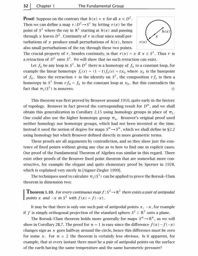
Proof: Suppose on the contrary that h(x) ≠ x for all x ∈ D2 .
Then we can define a map r :D2→S1 by letting r(x) be the
point of S1 where the ray in R2 starting at h(x) and passing
through x leaves D2 . Continuity of r is clear since small per-
turbations of x produce small perturbations of h(x) , hence
also small perturbations of the ray through these two points.
The crucial property of r , besides continuity, is that r(x) = x if x ∈ S1 . Thus r is
a retraction of D2 onto S1 . We will show that no such retraction can exist.
Let f0 be any loop in S1 . In D2 there is a homotopy of f0 to a constant loop, for
example the linear homotopy ft(s) = (1 − t)f0(s) + tx0 where x0 is the basepoint
of f0 . Since the retraction r is the identity on S1 , the composition rft is then a
homotopy in S1 from rf0 = f0 to the constant loop at x0 . But this contradicts the
fact that π1(S1) is nonzero. ⊔⊓
This theorem was first proved by Brouwer around 1910, quite early in the history
of topology. Brouwer in fact proved the corresponding result for Dn , and we shall
obtain this generalization in Corollary 2.15 using homology groups in place of π1 .
One could also use the higher homotopy group πn . Brouwer’s original proof used
neither homology nor homotopy groups, which had not been invented at the time.
Instead it used the notion of degree for maps Sn→Sn , which we shall define in §2.2
using homology but which Brouwer defined directly in more geometric terms.
These proofs are all arguments by contradiction, and so they show just the exis-
tence of fixed points without giving any clue as to how to find one in explicit cases.
Our proof of the Fundamental Theorem of Algebra was similar in this regard. There
exist other proofs of the Brouwer fixed point theorem that are somewhat more con-
structive, for example the elegant and quite elementary proof by Sperner in 1928,
which is explained very nicely in [Aigner-Ziegler 1999].
The techniques used to calculate π1(S1) can be applied to prove the Borsuk–Ulam
theorem in dimension two:
Theorem 1.10. For every continuous map f :S2→R2 there exists a pair of antipodal
points x and −x in S2 with f(x) = f(−x) .
It may be that there is only one such pair of antipodal points x , −x , for example
if f is simply orthogonal projection of the standard sphere S2⊂ R
3 onto a plane.
The Borsuk–Ulam theorem holds more generally for maps Sn→Rn , as we will
show in Corollary 2B.7. The proof for n = 1 is easy since the difference f(x)−f(−x)
changes sign as x goes halfway around the circle, hence this difference must be zero
for some x . For n ≥ 2 the theorem is certainly less obvious. Is it apparent, for
example, that at every instant there must be a pair of antipodal points on the surface
of the earth having the same temperature and the same barometric pressure?

Basic Constructions Section 1.1 33
The theorem says in particular that there is no one-to-one continuous map from
S2 to R2 , so S2 is not homeomorphic to a subspace of R2 , an intuitively obvious fact
that is not easy to prove directly.
Proof: If the conclusion is false for f :S2→R2 , we can define a map g :S2→S1 by
g(x) =(f(x) − f(−x)
)/|f(x) − f(−x)| . Define a loop η circling the equator of
S2⊂ R
3 by η(s) = (cos 2πs, sin 2πs,0) , and let h : I→S1 be the composed loop gη .
Since g(−x) = −g(x) , we have the relation h(s+ 1/2) = −h(s) for all s in the interval
[0, 1/2]. As we showed in the calculation of π1(S1) , the loop h can be lifted to a path
h : I→R . The equation h(s + 1/2) = −h(s) implies that h(s + 1/2) = h(s) +q/2 for
some odd integer q that might conceivably depend on s ∈ [0, 1/2]. But in fact q is
independent of s since by solving the equation h(s+1/2) = h(s)+q/2 for q we see that
q depends continuously on s ∈ [0, 1/2], so q must be a constant since it is constrained
to integer values. In particular, we have h(1) = h(1/2) +q/2 = h(0) + q. This means
that h represents q times a generator of π1(S1) . Since q is odd, we conclude that h
is not nullhomotopic. But h was the composition gη : I→S2→S1 , and η is obviously
nullhomotopic in S2 , so gη is nullhomotopic in S1 by composing a nullhomotopy of
η with g . Thus we have arrived at a contradiction. ⊔⊓
Corollary 1.11. Whenever S2 is expressed as the union of three closed sets A1 , A2 ,
and A3 , then at least one of these sets must contain a pair of antipodal points {x,−x} .
Proof: Let di :S2→R measure distance to Ai , that is, di(x) = infy∈Ai |x − y| . This
is a continuous function, so we may apply the Borsuk–Ulam theorem to the map
S2→R2 , x֏
(d1(x),d2(x)
), obtaining a pair of antipodal points x and −x with
d1(x) = d1(−x) and d2(x) = d2(−x) . If either of these two distances is zero, then
x and −x both lie in the same set A1 or A2 since these are closed sets. On the other
hand, if the distances from x and −x to A1 and A2 are both strictly positive, then
x and −x lie in neither A1 nor A2 so they must lie in A3 . ⊔⊓
To see that the number ‘three’ in this result is best possible, consider a sphere
inscribed in a tetrahedron. Projecting the four faces of the tetrahedron radially onto
the sphere, we obtain a cover of S2 by four closed sets, none of which contains a pair
of antipodal points.
Assuming the higher-dimensional version of the Borsuk–Ulam theorem, the same
arguments show that Sn cannot be covered by n + 1 closed sets without antipodal
pairs of points, though it can be covered by n+2 such sets, as the higher-dimensional
analog of a tetrahedron shows. Even the case n = 1 is somewhat interesting: If the
circle is covered by two closed sets, one of them must contain a pair of antipodal
points. This is of course false for nonclosed sets since the circle is the union of two
disjoint half-open semicircles.

34 Chapter 1 The Fundamental Group
The relation between the fundamental group of a product space and the funda-
mental groups of its factors is as simple as one could wish:
Proposition 1.12. π1(X×Y) is isomorphic to π1(X)×π1(Y ) if X and Y are path-
connected.
Proof: A basic property of the product topology is that a map f :Z→X×Y is con-
tinuous iff the maps g :Z→X and h :Z→Y defined by f(z) = (g(z),h(z)) are both
continuous. Hence a loop f in X×Y based at (x0, y0) is equivalent to a pair of loops
g in X and h in Y based at x0 and y0 respectively. Similarly, a homotopy ft of a loop
in X×Y is equivalent to a pair of homotopies gt and ht of the corresponding loops
in X and Y . Thus we obtain a bijection π1
(X×Y , (x0, y0)
)≈ π1(X,x0)×π1(Y ,y0) ,
[f ]֏ ([g], [h]) . This is obviously a group homomorphism, and hence an isomor-
phism. ⊔⊓
Example 1.13: The Torus. By the proposition we have an isomorphism π1(S1×S1) ≈
Z×Z . Under this isomorphism a pair (p, q) ∈ Z×Z corresponds to a loop that winds
p times around one S1 factor of the torus and q times around the
other S1 factor, for example the loop ωpq(s) = (ωp(s),ωq(s)) .
Interestingly, this loop can be knotted, as the figure shows for
the case p = 3, q = 2. The knots that arise in this fashion, the
so-called torus knots, are studied in Example 1.24.
More generally, the n dimensional torus, which is the product of n circles, has
fundamental group isomorphic to the product of n copies of Z . This follows by
induction on n .
Induced Homomorphisms
Suppose ϕ :X→Y is a map taking the basepoint x0 ∈ X to the basepoint y0 ∈ Y .
For brevity we write ϕ : (X,x0)→(Y ,y0) in this situation. Then ϕ induces a homo-
morphism ϕ∗ :π1(X,x0)→π1(Y ,y0) , defined by composing loops f : I→X based at
x0 with ϕ , that is, ϕ∗[f ] = [ϕf] . This induced map ϕ∗ is well-defined since a
homotopy ft of loops based at x0 yields a composed homotopy ϕft of loops based
at y0 , so ϕ∗[f0] = [ϕf0] = [ϕf1] =ϕ∗[f1] . Furthermore, ϕ∗ is a homomorphism
since ϕ(f g) = (ϕf) (ϕg) , both functions having the value ϕf(2s) for 0 ≤ s ≤ 1/2and the value ϕg(2s − 1) for 1/2 ≤ s ≤ 1.
Two basic properties of induced homomorphisms are:
(ϕψ)∗ =ϕ∗ψ∗ for a composition (X,x0)ψ-----→(Y ,y0)
ϕ-----→(Z, z0) .
11∗ = 11, which is a concise way of saying that the identity map 11 :X→X induces
the identity map 11 :π1(X,x0)→π1(X,x0) .
The first of these follows from the fact that composition of maps is associative, so
(ϕψ)f = ϕ(ψf) , and the second is obvious. These two properties of induced homo-
morphisms are what makes the fundamental group a functor. The formal definition
Basic Constructions Section 1.1 35
of a functor requires the introduction of certain other preliminary concepts, however,
so we postpone this until it is needed in §2.3.
As an application we can deduce easily that if ϕ is a homeomorphism with inverse
ψ then ϕ∗ is an isomorphism with inverse ψ∗ since ϕ∗ψ∗ = (ϕψ)∗ = 11∗ = 11
and similarly ψ∗ϕ∗ = 11. We will use this fact in the following calculation of the
fundamental groups of higher-dimensional spheres:
Proposition 1.14. π1(Sn) = 0 if n ≥ 2 .
The main step in the proof will be a general fact that will also play a key role in
the next section:
Lemma 1.15. If a space X is the union of a collection of path-connected open sets
Aα each containing the basepoint x0 ∈ X and if each intersection Aα ∩Aβ is path-
connected, then every loop in X at x0 is homotopic to a product of loops each of
which is contained in a single Aα .
Proof: Given a loop f : I→X at the basepoint x0 , we claim there is a partition 0 =
s0 < s1 < ··· < sm = 1 of I such that each subinterval [si−1, si] is mapped by f to
a single Aα . Namely, since f is continuous, each s ∈ I has an open neighborhood
Vs in I mapped by f to some Aα . We may in fact take Vs to be an interval whose
closure is mapped to a single Aα . Compactness of I implies that a finite number of
these intervals cover I . The endpoints of this finite set of intervals then define the
desired partition of I .
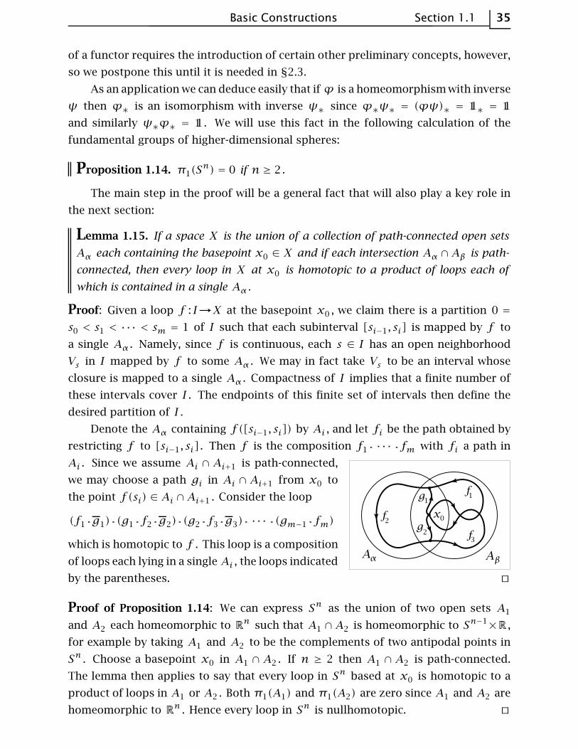
Denote the Aα containing f([si−1, si]) by Ai , and let fi be the path obtained by
restricting f to [si−1, si] . Then f is the composition f1 ··· fm with fi a path in
Ai . Since we assume Ai ∩ Ai+1 is path-connected,
we may choose a path gi in Ai ∩ Ai+1 from x0 to
the point f(si) ∈ Ai ∩Ai+1 . Consider the loop
(f1 g1) (g1 f2 g2) (g2 f3 g3) ··· (gm−1 fm)
which is homotopic to f . This loop is a composition
of loops each lying in a single Ai , the loops indicated
by the parentheses. ⊔⊓
Proof of Proposition 1.14: We can express Sn as the union of two open sets A1
and A2 each homeomorphic to Rn such that A1 ∩A2 is homeomorphic to Sn−1×R ,
for example by taking A1 and A2 to be the complements of two antipodal points in
Sn . Choose a basepoint x0 in A1 ∩ A2 . If n ≥ 2 then A1 ∩ A2 is path-connected.
The lemma then applies to say that every loop in Sn based at x0 is homotopic to a
product of loops in A1 or A2 . Both π1(A1) and π1(A2) are zero since A1 and A2 are
homeomorphic to Rn . Hence every loop in Sn is nullhomotopic. ⊔⊓

36 Chapter 1 The Fundamental Group
Corollary 1.16. R2 is not homeomorphic to Rn for n ≠ 2 .
Proof: Suppose f :R2→Rn is a homeomorphism. The case n = 1 is easily dis-
posed of since R2−{0} is path-connected but the homeomorphic space Rn − {f(0)}
is not path-connected when n = 1. When n > 2 we cannot distinguish R2− {0}
from Rn− {f(0)} by the number of path-components, but we can distinguish them
by their fundamental groups. Namely, for a point x in Rn , the complement Rn−{x}
is homeomorphic to Sn−1×R , so Proposition 1.12 implies that π1(R
n− {x}) is iso-
morphic to π1(Sn−1)×π1(R) ≈ π1(S
n−1) . Hence π1(Rn− {x}) is Z for n = 2 and
trivial for n > 2, using Proposition 1.14 in the latter case. ⊔⊓
The more general statement that Rm is not homeomorphic to Rn if m ≠ n can
be proved in the same way using either the higher homotopy groups or homology
groups. In fact, nonempty open sets in Rm and R
n can be homeomorphic only if
m = n , as we will show in Theorem 2.26 using homology.
Induced homomorphisms allow relations between spaces to be transformed into
relations between their fundamental groups. Here is an illustration of this principle:
Proposition 1.17. If a space X retracts onto a subspace A , then the homomorphism
i∗ :π1(A,x0)→π1(X,x0) induced by the inclusion i :A X is injective. If A is a
deformation retract of X , then i∗ is an isomorphism.
Proof: If r :X→A is a retraction, then ri = 11, hence r∗i∗ = 11, which implies that i∗is injective. If rt :X→X is a deformation retraction of X onto A , so r0 = 11, rt|A = 11,
and r1(X) ⊂ A , then for any loop f : I→X based at x0 ∈ A the composition rtf gives
a homotopy of f to a loop in A , so i∗ is also surjective. ⊔⊓
This gives another way of seeing that S1 is not a retract of D2 , a fact we showed
earlier in the proof of the Brouwer fixed point theorem, since the inclusion-induced
map π1(S1)→π1(D
2) is a homomorphism Z→0 that cannot be injective.
The exact group-theoretic analog of a retraction is a homomorphism ρ of a group
G onto a subgroup H such that ρ restricts to the identity on H . In the notation
above, if we identify π1(A) with its image under i∗ , then r∗ is such a homomorphism
from π1(X) onto the subgroup π1(A) . The existence of a retracting homomorphism
ρ :G→H is quite a strong condition on H . If H is a normal subgroup, it implies that
G is the direct product of H and the kernel of ρ . If H is not normal, then G is what
is called in group theory the semi-direct product of H and the kernel of ρ .
Recall from Chapter 0 the general definition of a homotopy as a family ϕt :X→Y ,
t ∈ I , such that the associated map Φ :X×I→Y ,Φ(x, t) = ϕt(x) , is continuous. If ϕttakes a subspace A ⊂ X to a subspace B ⊂ Y for all t , then we speak of a homotopy of
maps of pairs, ϕt : (X,A)→(Y , B) . In particular, a basepoint-preserving homotopy
Basic Constructions Section 1.1 37
ϕt : (X,x0)→(Y ,y0) is the case that ϕt(x0) = y0 for all t . Another basic property
of induced homomorphisms is their invariance under such homotopies:
If ϕt : (X,x0)→(Y ,y0) is a basepoint-preserving homotopy, then ϕ0∗ =ϕ1∗ .
This holds since ϕ0∗[f ] = [ϕ0f] = [ϕ1f] = ϕ1∗[f ] , the middle equality coming
from the homotopy ϕtf .
There is a notion of homotopy equivalence for spaces with basepoints. One says
(X,x0) ≃ (Y ,y0) if there are maps ϕ : (X,x0)→(Y ,y0) and ψ : (Y ,y0)→(X,x0)
with homotopies ϕψ ≃ 11 and ψϕ ≃ 11 through maps fixing the basepoints. In
this case the induced maps on π1 satisfy ϕ∗ψ∗ = (ϕψ)∗ = 11∗ = 11 and likewise
ψ∗ϕ∗ = 11, so ϕ∗ and ψ∗ are inverse isomorphisms π1(X,x0) ≈ π1(Y ,y0) . This
somewhat formal argument gives another proof that a deformation retraction induces
an isomorphism on fundamental groups, since if X deformation retracts onto A then
(X,x0) ≃ (A,x0) for any choice of basepoint x0 ∈ A .
Having to pay so much attention to basepoints when dealing with the fundamental
group is something of a nuisance. For homotopy equivalences one does not have to
be quite so careful, as the conditions on basepoints can actually be dropped:
Proposition 1.18. If ϕ :X→Y is a homotopy equivalence, then the induced homo-
morphism ϕ∗ :π1(X,x0)→π1
(Y ,ϕ(x0)
)is an isomorphism for all x0 ∈ X .
The proof will use a simple fact about homotopies that do not fix the basepoint:
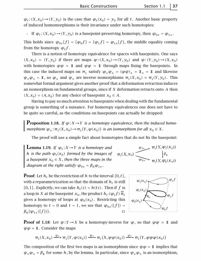
Lemma 1.19. If ϕt :X→Y is a homotopy and
h is the path ϕt(x0) formed by the images of
a basepoint x0 ∈ X , then the three maps in the
diagram at the right satisfy ϕ0∗ = βhϕ1∗ .
Proof: Let ht be the restriction of h to the interval [0, t] ,
with a reparametrization so that the domain of ht is still
[0,1] . Explicitly, we can take ht(s) = h(ts) . Then if f is
a loop in X at the basepoint x0 , the product ht (ϕtf) htgives a homotopy of loops at ϕ0(x0) . Restricting this
homotopy to t = 0 and t = 1, we see that ϕ0∗([f ]) =
βh(ϕ1∗([f ])
). ⊔⊓
Proof of 1.18: Let ψ :Y→X be a homotopy-inverse for ϕ , so that ϕψ ≃ 11 and
ψϕ ≃ 11. Consider the maps
π1(X,x0)ϕ∗------------→π1
(Y ,ϕ(x0)
) ψ∗------------→π1
(X,ψϕ(x0)
) ϕ∗------------→π1
(Y ,ϕψϕ(x0)
)
The composition of the first two maps is an isomorphism since ψϕ ≃ 11 implies that
ψ∗ϕ∗ = βh for some h , by the lemma. In particular, since ψ∗ϕ∗ is an isomorphism,

38 Chapter 1 The Fundamental Group
ϕ∗ is injective. The same reasoning with the second and third maps shows that ψ∗is injective. Thus the first two of the three maps are injections and their composition
is an isomorphism, so the first map ϕ∗ must be surjective as well as injective. ⊔⊓
Exercises
1. Show that composition of paths satisfies the following cancellation property: If
f0 g0 ≃ f1 g1 and g0 ≃ g1 then f0 ≃ f1 .
2. Show that the change-of-basepoint homomorphism βh depends only on the homo-
topy class of h .
3. For a path-connected space X , show that π1(X) is abelian iff all basepoint-change
homomorphisms βh depend only on the endpoints of the path h .
4. A subspace X ⊂ Rn is said to be star-shaped if there is a point x0 ∈ X such that,
for each x ∈ X , the line segment from x0 to x lies in X . Show that if a subspace
X ⊂ Rn is locally star-shaped, in the sense that every point of X has a star-shaped
neighborhood in X , then every path in X is homotopic in X to a piecewise linear
path, that is, a path consisting of a finite number of straight line segments traversed
at constant speed. Show this applies in particular when X is open or when X is a
union of finitely many closed convex sets.
5. Show that for a space X , the following three conditions are equivalent:
(a) Every map S1→X is homotopic to a constant map, with image a point.
(b) Every map S1→X extends to a map D2→X .
(c) π1(X,x0) = 0 for all x0 ∈ X .
Deduce that a space X is simply-connected iff all maps S1→X are homotopic. [In
this problem, ‘homotopic’ means ‘homotopic without regard to basepoints’.]
6. We can regard π1(X,x0) as the set of basepoint-preserving homotopy classes of
maps (S1, s0)→(X,x0) . Let [S1, X] be the set of homotopy classes of maps S1→X ,
with no conditions on basepoints. Thus there is a natural map Φ :π1(X,x0)→[S1, X]
obtained by ignoring basepoints. Show that Φ is onto if X is path-connected, and that
Φ([f ]) = Φ([g]) iff [f ] and [g] are conjugate in π1(X,x0) . Hence Φ induces a one-
to-one correspondence between [S1, X] and the set of conjugacy classes in π1(X) ,
when X is path-connected.
7. Define f :S1×I→S1
×I by f(θ, s) = (θ + 2πs, s) , so f restricts to the identity
on the two boundary circles of S1×I . Show that f is homotopic to the identity by
a homotopy ft that is stationary on one of the boundary circles, but not by any ho-
motopy ft that is stationary on both boundary circles. [Consider what f does to the
path s֏ (θ0, s) for fixed θ0 ∈ S1 .]
8. Does the Borsuk–Ulam theorem hold for the torus? In other words, for every map
f :S1×S1→R
2 must there exist (x,y) ∈ S1×S1 such that f(x,y) = f(−x,−y)?
Basic Constructions Section 1.1 39
9. Let A1 , A2 , A3 be compact sets in R3 . Use the Borsuk–Ulam theorem to show
that there is one plane P ⊂ R3 that simultaneously divides each Ai into two pieces of
equal measure.
10. From the isomorphism π1
(X×Y , (x0, y0)
)≈ π1(X,x0)×π1(Y ,y0) it follows that
loops in X×{y0} and {x0}×Y represent commuting elements of π1
(X×Y , (x0, y0)
).
Construct an explicit homotopy demonstrating this.
11. If X0 is the path-component of a space X containing the basepoint x0 , show that
the inclusion X0X induces an isomorphism π1(X0, x0)→π1(X,x0) .
12. Show that every homomorphism π1(S1)→π1(S
1) can be realized as the induced
homomorphism ϕ∗ of a map ϕ :S1→S1 .
13. Given a space X and a path-connected subspace A containing the basepoint x0 ,
show that the map π1(A,x0)→π1(X,x0) induced by the inclusion AX is surjective
iff every path in X with endpoints in A is homotopic to a path in A .
14. Show that the isomorphism π1(X×Y) ≈ π1(X)×π1(Y ) in Proposition 1.12 is
given by [f ]֏ (p1∗([f ]), p2∗([f ])) where p1 and p2 are the projections of X×Y
onto its two factors.
15. Given a map f :X→Y and a path h : I→Xfrom x0 to x1 , show that f∗βh = βfhf∗ in the
diagram at the right.
16. Show that there are no retractions r :X→A in the following cases:
(a) X = R3 with A any subspace homeomorphic to S1 .
(b) X = S1×D2 with A its boundary torus S1
×S1 .
(c) X = S1×D2 and A the circle shown in the figure.
(d) X = D2∨D2 with A its boundary S1
∨ S1 .
(e) X a disk with two points on its boundary identified and A its boundary S1∨ S1 .
(f) X the Mobius band and A its boundary circle.
17. Construct infinitely many nonhomotopic retractions S1∨ S1→S1 .
18. Using Lemma 1.15, show that if a space X is obtained from a path-connected
subspace A by attaching a cell en with n ≥ 2, then the inclusion A X induces a
surjection on π1 . Apply this to show:
(a) The wedge sum S1∨ S2 has fundamental group Z .
(b) For a path-connected CW complex X the inclusion map X1X of its 1 skeleton
induces a surjection π1(X1)→π1(X) . [For the case that X has infinitely many
cells, see Proposition A.1 in the Appendix.]
19. Show that if X is a path-connected 1 dimensional CW complex with basepoint x0
a 0 cell, then every loop in X is homotopic to a loop consisting of a finite sequence of
edges traversed monotonically. [See the proof of Lemma 1.15. This exercise gives an
elementary proof that π1(S1) is cyclic generated by the standard loop winding once
40 Chapter 1 The Fundamental Group
around the circle. The more difficult part of the calculation of π1(S1) is therefore the
fact that no iterate of this loop is nullhomotopic.]
20. Suppose ft :X→X is a homotopy such that f0 and f1 are each the identity map.
Use Lemma 1.19 to show that for any x0 ∈ X , the loop ft(x0) represents an element of
the center of π1(X,x0) . [One can interpret the result as saying that a loop represents
an element of the center of π1(X) if it extends to a loop of maps X→X .]
The van Kampen theorem gives a method for computing the fundamental groups
of spaces that can be decomposed into simpler spaces whose fundamental groups are
already known. By systematic use of this theorem one can compute the fundamental
groups of a very large number of spaces. We shall see for example that for every group
G there is a space XG whose fundamental group is isomorphic to G .
To give some idea of how one might hope to compute fundamental groups by
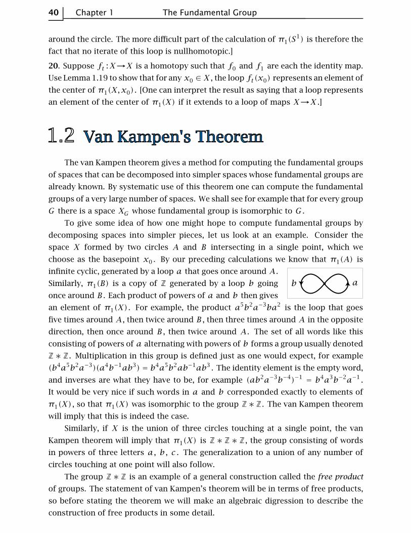
decomposing spaces into simpler pieces, let us look at an example. Consider the
space X formed by two circles A and B intersecting in a single point, which we
choose as the basepoint x0 . By our preceding calculations we know that π1(A) is
infinite cyclic, generated by a loop a that goes once around A .
Similarly, π1(B) is a copy of Z generated by a loop b going
once around B . Each product of powers of a and b then gives
an element of π1(X) . For example, the product a5b2a−3ba2 is the loop that goes
five times around A , then twice around B , then three times around A in the opposite
direction, then once around B , then twice around A . The set of all words like this
consisting of powers of a alternating with powers of b forms a group usually denoted
Z ∗ Z . Multiplication in this group is defined just as one would expect, for example
(b4a5b2a−3)(a4b−1ab3) = b4a5b2ab−1ab3 . The identity element is the empty word,
and inverses are what they have to be, for example (ab2a−3b−4)−1= b4a3b−2a−1 .
It would be very nice if such words in a and b corresponded exactly to elements of
π1(X) , so that π1(X) was isomorphic to the group Z∗ Z . The van Kampen theorem
will imply that this is indeed the case.
Similarly, if X is the union of three circles touching at a single point, the van
Kampen theorem will imply that π1(X) is Z ∗ Z ∗ Z , the group consisting of words
in powers of three letters a , b , c . The generalization to a union of any number of
circles touching at one point will also follow.
The group Z ∗ Z is an example of a general construction called the free product
of groups. The statement of van Kampen’s theorem will be in terms of free products,
so before stating the theorem we will make an algebraic digression to describe the
construction of free products in some detail.

Van Kampen’s Theorem Section 1.2 41
Free Products of Groups
Suppose one is given a collection of groups Gα and one wishes to construct a
single group containing all these groups as subgroups. One way to do this would be
to take the product group∏αGα , whose elements can be regarded as the functions
α֏ gα ∈ Gα . Or one could restrict to functions taking on nonidentity values at
most finitely often, forming the direct sum⊕αGα . Both these constructions produce
groups containing all the Gα ’s as subgroups, but with the property that elements of
different subgroups Gα commute with each other. In the realm of nonabelian groups
this commutativity is unnatural, and so one would like a ‘nonabelian’ version of∏αGα
or⊕αGα . Since the sum
⊕αGα is smaller and presumably simpler than
∏αGα , it
should be easier to construct a nonabelian version of⊕αGα , and this is what the free
product ∗αGα achieves.
Here is the precise definition. As a set, the free product ∗αGα consists of all
words g1g2 ···gm of arbitrary finite length m ≥ 0, where each letter gi belongs to
a group Gαi and is not the identity element of Gαi , and adjacent letters gi and gi+1
belong to different groups Gα , that is, αi ≠ αi+1 . Words satisfying these conditions
are called reduced , the idea being that unreduced words can always be simplified to
reduced words by writing adjacent letters that lie in the same Gαi as a single letter and
by canceling trivial letters. The empty word is allowed, and will be the identity element
of ∗αGα . The group operation in ∗αGα is juxtaposition, (g1 ···gm)(h1 ···hn) =
g1 ···gmh1 ···hn . This product may not be reduced, however: If gm and h1 belong
to the same Gα , they should be combined into a single letter (gmh1) according to the
multiplication in Gα , and if this new letter gmh1 happens to be the identity of Gα , it
should be canceled from the product. This may allow gm−1 and h2 to be combined,
and possibly canceled too. Repetition of this process eventually produces a reduced
word. For example, in the product (g1 ···gm)(g−1m ···g
−11 ) everything cancels and
we get the identity element of ∗αGα , the empty word.
Verifying directly that this multiplication is associative would be rather tedious,
but there is an indirect approach that avoids most of the work. Let W be the set of
reduced words g1 ···gm as above, including the empty word. To each g ∈ Gα we
associate the function Lg :W→W given by multiplication on the left, Lg(g1 ···gm) =
gg1 ···gm where we combine g with g1 if g1 ∈ Gα to make gg1 ···gm a reduced
word. A key property of the association g֏ Lg is the formula Lgg′ = LgLg′ for
g,g′ ∈ Gα , that is, g(g′(g1 ···gm)) = (gg′)(g1 ···gm) . This special case of asso-
ciativity follows rather trivially from associativity in Gα . The formula Lgg′ = LgLg′
implies that Lg is invertible with inverse Lg−1 . Therefore the association g֏ Lg de-
fines a homomorphism from Gα to the group P(W) of all permutations of W . More
generally, we can define L :W→P(W) by L(g1 ···gm) = Lg1···Lgm for each reduced
word g1 ···gm . This function L is injective since the permutation L(g1 ···gm) sends
the empty word to g1 ···gm . The product operation in W corresponds under L to
42 Chapter 1 The Fundamental Group
composition in P(W) , because of the relation Lgg′ = LgLg′ . Since composition in
P(W) is associative, we conclude that the product in W is associative.
In particular, we have the free product Z ∗ Z as described earlier. This is an
example of a free group, the free product of any number of copies of Z , finite or
infinite. The elements of a free group are uniquely representable as reduced words in
powers of generators for the various copies of Z , with one generator for each Z , just
as in the case of Z∗Z . These generators are called a basis for the free group, and the
number of basis elements is the rank of the free group. The abelianization of a free
group is a free abelian group with basis the same set of generators, so since the rank
of a free abelian group is well-defined, independent of the choice of basis, the same
is true for the rank of a free group.
An interesting example of a free product that is not a free group is Z2 ∗ Z2 . This
is like Z∗Z but simpler since a2= e = b2 , so powers of a and b are not needed, and
Z2∗Z2 consists of just the alternating words in a and b : a , b , ab , ba , aba , bab ,
abab , baba , ababa, ··· , together with the empty word. The structure of Z2 ∗ Z2
can be elucidated by looking at the homomorphism ϕ :Z2 ∗ Z2→Z2 associating to
each word its length mod 2. Obviously ϕ is surjective, and its kernel consists of the
words of even length. These form an infinite cyclic subgroup generated by ab since
ba = (ab)−1 in Z2 ∗ Z2 . In fact, Z2 ∗ Z2 is the semi-direct product of the subgroups
Z and Z2 generated by ab and a , with the conjugation relation a(ab)a−1= (ab)−1 .
This group is sometimes called the infinite dihedral group.
For a general free product ∗αGα , each group Gα is naturally identified with a
subgroup of ∗αGα , the subgroup consisting of the empty word and the nonidentity
one-letter words g ∈ Gα . From this viewpoint the empty word is the common iden-
tity element of all the subgroups Gα , which are otherwise disjoint. A consequence
of associativity is that any product g1 ···gm of elements gi in the groups Gα has a
unique reduced form, the element of ∗αGα obtained by performing the multiplica-
tions in any order. Any sequence of reduction operations on an unreduced product
g1 ···gm , combining adjacent letters gi and gi+1 that lie in the same Gα or canceling
a gi that is the identity, can be viewed as a way of inserting parentheses into g1 ···gmand performing the resulting sequence of multiplications. Thus associativity implies
that any two sequences of reduction operations performed on the same unreduced
word always yield the same reduced word.
A basic property of the free product ∗αGα is that any collection of homomor-
phisms ϕα :Gα→H extends uniquely to a homomorphism ϕ :∗αGα→H . Namely,
the value of ϕ on a word g1 ···gn with gi ∈ Gαi must be ϕα1(g1) ···ϕαn(gn) , and
using this formula to define ϕ gives a well-defined homomorphism since the process
of reducing an unreduced product in ∗αGα does not affect its image under ϕ . For
example, for a free product G∗H the inclusions GG×H and HG×H induce
a surjective homomorphism G ∗H→G×H .

Van Kampen’s Theorem Section 1.2 43
The van Kampen Theorem
Suppose a space X is decomposed as the union of a collection of path-connected
open subsets Aα , each of which contains the basepoint x0 ∈ X . By the remarks in the
preceding paragraph, the homomorphisms jα :π1(Aα)→π1(X) induced by the inclu-
sions Aα X extend to a homomorphism Φ :∗απ1(Aα)→π1(X) . The van Kampen
theorem will say that Φ is very often surjective, but we can expect Φ to have a nontriv-
ial kernel in general. For if iαβ :π1(Aα∩Aβ)→π1(Aα) is the homomorphism induced
by the inclusion Aα ∩ Aβ Aα then jαiαβ = jβiβα , both these compositions being
induced by the inclusion Aα ∩Aβ X , so the kernel of Φ contains all the elements
of the form iαβ(ω)iβα(ω)−1 for ω ∈ π1(Aα ∩ Aβ) . Van Kampen’s theorem asserts
that under fairly broad hypotheses this gives a full description of Φ :
Theorem 1.20. If X is the union of path-connected open sets Aα each containing
the basepoint x0 ∈ X and if each intersection Aα ∩ Aβ is path-connected, then the
homomorphism Φ :∗απ1(Aα)→π1(X) is surjective. If in addition each intersection
Aα ∩ Aβ ∩ Aγ is path-connected, then the kernel of Φ is the normal subgroup N
generated by all elements of the form iαβ(ω)iβα(ω)−1 for ω ∈ π1(Aα ∩ Aβ) , and
hence Φ induces an isomorphism π1(X) ≈ ∗απ1(Aα)/N .
Example 1.21: Wedge Sums. In Chapter 0 we defined the wedge sum∨αXα of a
collection of spaces Xα with basepoints xα ∈ Xα to be the quotient space of the
disjoint union∐αXα in which all the basepoints xα are identified to a single point.
If each xα is a deformation retract of an open neighborhood Uα in Xα , then Xα is
a deformation retract of its open neighborhood Aα = Xα∨β≠αUβ . The intersection
of two or more distinct Aα ’s is∨αUα , which deformation retracts to a point. Van
Kampen’s theorem then implies that Φ :∗απ1(Xα)→π1(∨αXα) is an isomorphism.
Thus for a wedge sum∨αS
1α of circles, π1(
∨αS
1α) is a free group, the free product
of copies of Z , one for each circle S1α . In particular, π1(S
1∨S1) is the free group Z∗Z ,
as in the example at the beginning of this section.
It is true more generally that the fundamental group of any connected graph is
free, as we show in §1.A. Here is an example illustrating the general technique.
Example 1.22. Let X be the graph shown in the figure, consist-
ing of the twelve edges of a cube. The seven heavily shaded edges
form a maximal tree T ⊂ X , a contractible subgraph containing all
the vertices of X . We claim that π1(X) is the free product of five
copies of Z , one for each edge not in T . To deduce this from van
Kampen’s theorem, choose for each edge eα of X − T an open neighborhood Aα of
T ∪ eα in X that deformation retracts onto T ∪ eα . The intersection of two or more
Aα ’s deformation retracts onto T , hence is contractible. The Aα ’s form a cover of
X satisfying the hypotheses of van Kampen’s theorem, and since the intersection of

44 Chapter 1 The Fundamental Group
any two of them is simply-connected we obtain an isomorphism π1(X) ≈ ∗απ1(Aα) .
Each Aα deformation retracts onto a circle, so π1(X) is free on five generators, as
claimed. As explicit generators we can choose for each edge eα of X − T a loop fαthat starts at a basepoint in T , travels in T to one end of eα , then across eα , then
back to the basepoint along a path in T .
Van Kampen’s theorem is often applied when there are just two sets Aα and Aβ in
the cover of X , so the condition on triple intersections Aα∩Aβ∩Aγ is superfluous and
one obtains an isomorphism π1(X) ≈(π1(Aα) ∗ π1(Aβ)
)/N , under the assumption
that Aα ∩ Aβ is path-connected. The proof in this special case is virtually identical
with the proof in the general case, however.
One can see that the intersections Aα ∩ Aβ need to be path-connected by con-
sidering the example of S1 decomposed as the union of two open arcs. In this case
Φ is not surjective. For an example showing that triple intersections Aα ∩ Aβ ∩ Aγneed to be path-connected, let X be the suspension of three points a , b , c , and let
Aα, Aβ , and Aγ be the complements of these three points. The theo-
rem does apply to the covering {Aα, Aβ} , so there are isomorphisms
π1(X) ≈ π1(Aα) ∗ π1(Aβ) ≈ Z ∗ Z since Aα ∩ Aβ is contractible.
If we tried to use the covering {Aα, Aβ, Aγ} , which has each of the
twofold intersections path-connected but not the triple intersection, then we would
get π1(X) ≈ Z ∗ Z ∗ Z , but this is not isomorphic to Z ∗ Z since it has a different
abelianization.
Proof of van Kampen’s theorem: We have already proved the first part of the theorem
concerning surjectivity of Φ in Lemma 1.15. The harder part of the proof is to show
that the kernel of Φ is N . It may clarify matters to introduce some terminology. By a
factorization of an element [f ] ∈ π1(X) we shall mean a formal product [f1] ··· [fk]
where:
Each fi is a loop in some Aα at the basepoint x0 , and [fi] ∈ π1(Aα) is the
homotopy class of fi .
The loop f is homotopic to f1 ··· fk in X .
A factorization of [f ] is thus a word in ∗απ1(Aα) , possibly unreduced, that is
mapped to [f ] by Φ . Surjectivity of Φ is equivalent to saying that every [f ] ∈ π1(X)
has a factorization.
We will be concerned with the uniqueness of factorizations. Call two factoriza-
tions of [f ] equivalent if they are related by a sequence of the following two sorts of
moves or their inverses:
Combine adjacent terms [fi][fi+1] into a single term [fi fi+1] if [fi] and [fi+1]
lie in the same group π1(Aα) .
Regard the term [fi] ∈ π1(Aα) as lying in the group π1(Aβ) rather than π1(Aα)
if fi is a loop in Aα ∩Aβ .

Van Kampen’s Theorem Section 1.2 45
The first move does not change the element of ∗απ1(Aα) defined by the factorization.
The second move does not change the image of this element in the quotient group
Q = ∗απ1(Aα)/N , by the definition of N . So equivalent factorizations give the same
element of Q .
If we can show that any two factorizations of [f ] are equivalent, this will say that
the map Q→π1(X) induced by Φ is injective, hence the kernel of Φ is exactly N , and
the proof will be complete.
Let [f1] ··· [fk] and [f ′1] ··· [f′ℓ] be two factorizations of [f ] . The composed
paths f1 ··· fk and f ′1 ··· f ′ℓ are then homotopic, so let F : I×I→X be a homo-
topy from f1 ··· fk to f ′1 ··· f ′ℓ . There exist partitions 0 = s0 < s1 < ··· < sm = 1
and 0 = t0 < t1 < ··· < tn = 1 such that each rectangle Rij = [si−1, si]×[tj−1, tj]
is mapped by F into a single Aα , which we label Aij . These partitions may be ob-
tained by covering I×I by finitely many rectangles [a, b]×[c, d] each mapping to a
single Aα , using a compactness argument, then partitioning I×I by the union of all
the horizontal and vertical lines containing edges of these rectangles. We may assume
the s partition subdivides the partitions giving the products
f1 ··· fk and f ′1 ··· f ′ℓ . Since F maps a neighborhood
of Rij to Aij , we may perturb the vertical sides of the rect-
angles Rij so that each point of I×I lies in at most three
Rij ’s. We may assume there are at least three rows of rect-
angles, so we can do this perturbation just on the rectangles
in the intermediate rows, leaving the top and bottom rows unchanged. Let us relabel
the new rectangles R1, R2, ··· , Rmn , ordering them as in the figure.
If γ is a path in I×I from the left edge to the right edge, then the restriction F ||γ
is a loop at the basepoint x0 since F maps both the left and right edges of I×I to x0 .
Let γr be the path separating the first r rectangles R1, ··· , Rr from the remaining
rectangles. Thus γ0 is the bottom edge of I×I and γmn is the top edge. We pass
from γr to γr+1 by pushing across the rectangle Rr+1 .
Let us call the corners of the Rr ’s vertices. For each vertex v with F(v) ≠ x0
we can choose a path gv from x0 to F(v) that lies in the intersection of the two
or three Aij ’s corresponding to the Rr ’s containing v , since we assume the inter-
section of any two or three Aij ’s is path-connected. Then we obtain a factorization
of [F ||γr ] by inserting the appropriate paths gvgv into F ||γr at successive vertices,
as in the proof of surjectivity of Φ in Lemma 1.15. This factorization depends on
certain choices, since the loop corresponding to a segment between two successive
vertices can lie in two different Aij ’s when there are two different rectangles Rij con-
taining this edge. Different choices of these Aij ’s change the factorization of [F ||γr ]
to an equivalent factorization, however. Furthermore, the factorizations associated
to successive paths γr and γr+1 are equivalent since pushing γr across Rr+1 to γr+1
changes F ||γr to F ||γr+1 by a homotopy within the Aij corresponding to Rr+1 , and
46 Chapter 1 The Fundamental Group
we can choose this Aij for all the segments of γr and γr+1 in Rr+1 .
We can arrange that the factorization associated to γ0 is equivalent to the factor-
ization [f1] ··· [fk] by choosing the path gv for each vertex v along the lower edge
of I×I to lie not just in the two Aij ’s corresponding to the Rs ’s containing v , but also
to lie in the Aα for the fi containing v in its domain. In case v is the common end-
point of the domains of two consecutive fi ’s we have F(v) = x0 , so there is no need
to choose a gv for such v ’s. In similar fashion we may assume that the factorization
associated to the final γmn is equivalent to [f ′1] ··· [f′ℓ] . Since the factorizations as-
sociated to all the γr ’s are equivalent, we conclude that the factorizations [f1] ··· [fk]
and [f ′1] ··· [f′ℓ] are equivalent. ⊔⊓
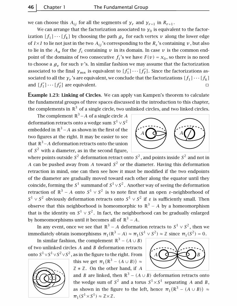
Example 1.23: Linking of Circles. We can apply van Kampen’s theorem to calculate
the fundamental groups of three spaces discussed in the introduction to this chapter,
the complements in R3 of a single circle, two unlinked circles, and two linked circles.
The complement R3−A of a single circle A
deformation retracts onto a wedge sum S1∨S2
embedded in R3−A as shown in the first of the
two figures at the right. It may be easier to see
that R3−A deformation retracts onto the union
of S2 with a diameter, as in the second figure,
where points outside S2 deformation retract onto S2 , and points inside S2 and not in
A can be pushed away from A toward S2 or the diameter. Having this deformation
retraction in mind, one can then see how it must be modified if the two endpoints
of the diameter are gradually moved toward each other along the equator until they
coincide, forming the S1 summand of S1∨S2 . Another way of seeing the deformation
retraction of R3− A onto S1
∨ S2 is to note first that an open ε neighborhood of
S1∨ S2 obviously deformation retracts onto S1
∨ S2 if ε is sufficiently small. Then
observe that this neighborhood is homeomorphic to R3− A by a homeomorphism
that is the identity on S1∨ S2 . In fact, the neighborhood can be gradually enlarged
by homeomorphisms until it becomes all of R3−A .
In any event, once we see that R3− A deformation retracts to S1
∨ S2 , then we
immediately obtain isomorphisms π1(R3−A) ≈ π1(S
1∨ S2) ≈ Z since π1(S
2) = 0.
In similar fashion, the complement R3− (A ∪ B)
of two unlinked circles A and B deformation retracts
onto S1∨S1
∨S2∨S2 , as in the figure to the right. From
this we get π1
(R
3− (A ∪ B)
)≈
Z ∗ Z . On the other hand, if A
and B are linked, then R3− (A ∪ B) deformation retracts onto
the wedge sum of S2 and a torus S1×S1 separating A and B ,
as shown in the figure to the left, hence π1
(R
3− (A ∪ B)
)≈
π1(S1×S1) ≈ Z×Z .

Van Kampen’s Theorem Section 1.2 47
Example 1.24: Torus Knots. For relatively prime positive integers m and n , the
torus knot K = Km,n ⊂ R3 is the image of the embedding f :S1→S1
×S1⊂ R
3 ,
f(z) = (zm, zn) , where the torus S1×S1 is embedded in R
3 in the standard way.
The knot K winds around the torus a total of m
times in the longitudinal direction and n times in
the meridional direction, as shown in the figure for
the cases (m,n) = (2,3) and (3,4) . One needs to
assume that m and n are relatively prime in order
for the map f to be injective. Without this assumption f would be d–to–1 where
d is the greatest common divisor of m and n , and the image of f would be the
knot Km/d,n/d . One could also allow negative values for m or n , but this would only
change K to a mirror-image knot.
Let us compute π1(R3−K) . It is slightly easier to do the calculation with R3 re-
placed by its one-point compactification S3 . An application of van Kampen’s theorem
shows that this does not affect π1 . Namely, write S3−K as the union of R3
−K and
an open ball B formed by the compactification point together with the complement of
a large closed ball in R3 containing K . Both B and B∩(R3−K) are simply-connected,
the latter space being homeomorphic to S2×R . Hence van Kampen’s theorem implies
that the inclusion R3−K S3
−K induces an isomorphism on π1 .
We compute π1(S3−K) by showing that it deformation retracts onto a 2 dimen-
sional complex X = Xm,n homeomorphic to the quotient space of a cylinder S1×I
under the identifications (z,0) ∼ (e2πi/mz,0) and (z,1) ∼ (e2πi/nz,1) . If we let Xmand Xn be the two halves of X formed by the quotients of S1
×[0, 1/2] and S1×[1/2,1],
then Xm and Xn are the mapping cylinders of z֏zm and z֏zn . The intersection
Xm ∩ Xn is the circle S1×{1/2}, the domain end of each mapping cylinder.
To obtain an embedding of X in S3− K as a deformation retract we will use the
standard decomposition of S3 into two solid tori S1×D2 and D2
×S1 , the result of
regarding S3 as ∂D4= ∂(D2
×D2) = ∂D2×D2
∪ D2×∂D2 . Geometrically, the first
solid torus S1×D2 can be identified with the compact region in R
3 bounded by the
standard torus S1×S1 containing K , and the second solid torus D2
×S1 is then the
closure of the complement of the first solid torus, together with the compactification
point at infinity. Notice that meridional circles in S1×S1 bound disks in the first solid
torus, while it is longitudinal circles that bound disks in the second solid torus.
In the first solid torus, K intersects each of the meridian
circles {x}×∂D2 in m equally spaced points, as indicated in
the figure at the right, which shows a meridian disk {x}×D2 .
These m points can be separated by a union of m radial line
segments. Letting x vary, these radial segments then trace out
a copy of the mapping cylinder Xm in the first solid torus. Sym-
metrically, there is a copy of the other mapping cylinder Xn in the second solid torus.
48 Chapter 1 The Fundamental Group
The complement of K in the first solid torus deformation retracts onto Xm by flowing
within each meridian disk as shown. In similar fashion the complement of K in the
second solid torus deformation retracts onto Xn . These two deformation retractions
do not agree on their common domain of definition S1×S1
− K , but this is easy to
correct by distorting the flows in the two solid tori so that in S1×S1
− K both flows
are orthogonal to K . After this modification we now have a well-defined deformation
retraction of S3− K onto X . Another way of describing the situation would be to
say that for an open ε neighborhood N of K bounded by a torus T , the complement
S3−N is the mapping cylinder of a map T→X .
To compute π1(X) we apply van Kampen’s theorem to the decomposition of X
as the union of Xm and Xn , or more properly, open neighborhoods of these two
sets that deformation retract onto them. Both Xm and Xn are mapping cylinders
that deformation retract onto circles, and Xm ∩ Xn is a circle, so all three of these
spaces have fundamental group Z . A loop in Xm ∩ Xn representing a generator of
π1(Xm∩Xn) is homotopic in Xm to a loop representing m times a generator, and in
Xn to a loop representing n times a generator. Van Kampen’s theorem then says that
π1(X) is the quotient of the free group on generators a and b obtained by factoring
out the normal subgroup generated by the element amb−n .
Let us denote by Gm,n this group π1(Xm,n) defined by two generators a and
b and one relation am = bn . If m or n is 1, then Gm,n is infinite cyclic since in
these cases the relation just expresses one generator as a power of the other. To
describe the structure of Gm,n when m,n > 1 let us first compute the center of
Gm,n , the subgroup consisting of elements that commute with all elements of Gm,n .
The element am = bn commutes with a and b , so the cyclic subgroup C generated
by this element lies in the center. In particular, C is a normal subgroup, so we can
pass to the quotient group Gm,n/C , which is the free product Zm ∗ Zn . According
to Exercise 1 at the end of this section, a free product of nontrivial groups has trivial
center. From this it follows that C is exactly the center of Gm,n . As we will see in
Example 1.44, the elements a and b have infinite order in Gm,n , so C is infinite cyclic,
but we will not need this fact here.
We will show now that the integers m and n are uniquely determined by the
group Zm ∗ Zn , hence also by Gm,n . The abelianization of Zm ∗ Zn is Zm×Zn , of
order mn , so the product mn is uniquely determined by Zm ∗ Zn . To determine m
and n individually, we use another assertion from Exercise 1 at the end of the section,
that all torsion elements of Zm∗Zn are conjugate to elements of one of the subgroups
Zm and Zn , hence have order dividing m or n . Thus the maximum order of torsion
elements of Zm ∗ Zn is the larger of m and n . The larger of these two numbers is
therefore uniquely determined by the group Zm∗Zn , hence also the smaller since the
product is uniquely determined.
The preceding analysis of π1(Xm,n) did not need the assumption that m and n

Van Kampen’s Theorem Section 1.2 49
are relatively prime, which was used only to relate Xm,n to torus knots. An interesting
fact is that Xm,n can be embedded in R3 only when m and n are relatively prime.
This is shown in the remarks following Corollary 3.45. For example, X2,2 is the Klein
bottle since it is the union of two copies of the Mobius band X2 with their boundary
circles identified, so this nonembeddability statement generalizes the fact that the
Klein bottle cannot be embedded in R3 .
An algorithm for computing a presentation for π1(R3−K) for an arbitrary smooth
or piecewise linear knot K is described in the exercises, but the problem of determin-
ing when two of these fundamental groups are isomorphic is generally much more
difficult than in the special case of torus knots.
Example 1.25: The Shrinking Wedge of Circles. Consider the sub-
space X ⊂ R2 that is the union of the circles Cn of radius 1/n and
center (1/n,0) for n = 1,2, ··· . At first glance one might confuse
X with the wedge sum of an infinite sequence of circles, but we will
show that X has a much larger fundamental group than the wedge
sum. Consider the retractions rn :X→Cn collapsing all Ci ’s except Cn to the origin.
Each rn induces a surjection ρn :π1(X)→π1(Cn) ≈ Z , where we take the origin as
the basepoint. The product of the ρn ’s is a homomorphism ρ :π1(X)→∏∞Z to the
direct product (not the direct sum) of infinitely many copies of Z , and ρ is surjective
since for every sequence of integers kn we can construct a loop f : I→X that wraps
kn times around Cn in the time interval [1− 1/n,1−1/n+1]. This infinite composition
of loops is certainly continuous at each time less than 1, and it is continuous at time
1 since every neighborhood of the basepoint in X contains all but finitely many of the
circles Cn . Since π1(X) maps onto the uncountable group∏∞Z , it is uncountable.
On the other hand, the fundamental group of a wedge sum of countably many circles
is countably generated, hence countable.
The group π1(X) is actually far more complicated than∏∞Z . For one thing,
it is nonabelian, since the retraction X→C1 ∪ ··· ∪ Cn that collapses all the circles
smaller than Cn to the basepoint induces a surjection from π1(X) to a free group on
n generators. For a complete description of π1(X) see [Cannon & Conner 2000].
It is a theorem of [Shelah 1988] that for a path-connected, locally path-connected
compact metric space X , π1(X) is either finitely generated or uncountable.
Applications to Cell Complexes
For the remainder of this section we shall be interested in cell complexes, and in
particular in how the fundamental group is affected by attaching 2 cells.
Suppose we attach a collection of 2 cells e2α to a path-connected space X via maps
ϕα :S1→X , producing a space Y . If s0 is a basepoint of S1 then ϕα determines a loop
at ϕα(s0) that we shall call ϕα , even though technically loops are maps I→X rather
than S1→X . For different α ’s the basepoints ϕα(s0) of these loops ϕα may not all
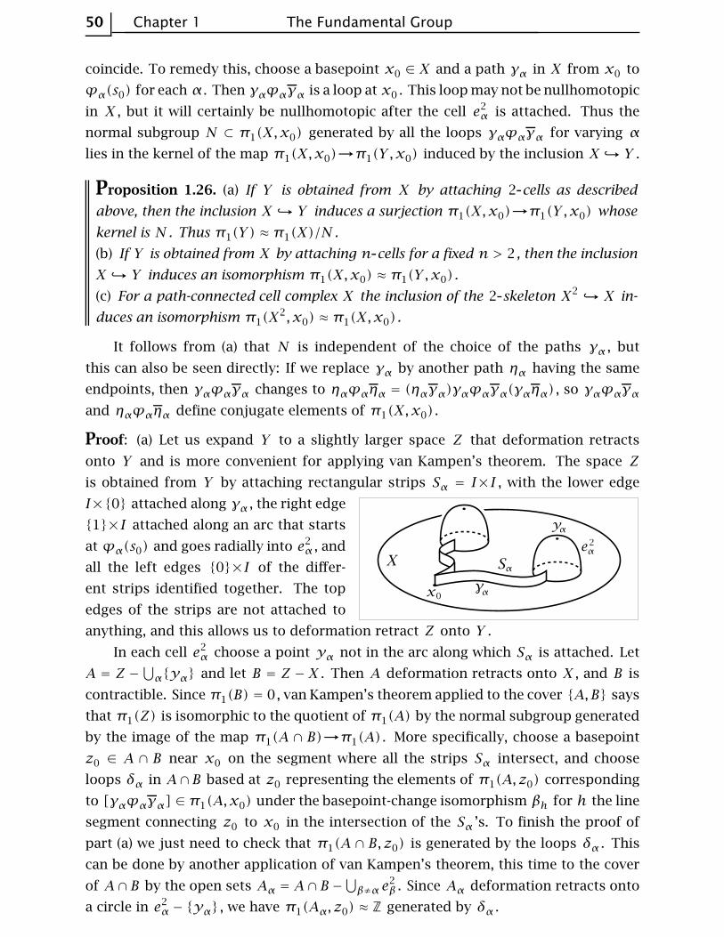
50 Chapter 1 The Fundamental Group
coincide. To remedy this, choose a basepoint x0 ∈ X and a path γα in X from x0 to
ϕα(s0) for each α . Then γαϕαγα is a loop at x0 . This loop may not be nullhomotopic
in X , but it will certainly be nullhomotopic after the cell e2α is attached. Thus the
normal subgroup N ⊂ π1(X,x0) generated by all the loops γαϕαγα for varying α
lies in the kernel of the map π1(X,x0)→π1(Y ,x0) induced by the inclusion X Y .
Proposition 1.26. (a) If Y is obtained from X by attaching 2 cells as described
above, then the inclusion X Y induces a surjection π1(X,x0)→π1(Y ,x0) whose
kernel is N . Thus π1(Y ) ≈ π1(X)/N .
(b) If Y is obtained from X by attaching n cells for a fixed n > 2 , then the inclusion
X Y induces an isomorphism π1(X,x0) ≈ π1(Y ,x0) .
(c) For a path-connected cell complex X the inclusion of the 2 skeleton X2 X in-
duces an isomorphism π1(X2, x0) ≈ π1(X,x0) .
It follows from (a) that N is independent of the choice of the paths γα , but
this can also be seen directly: If we replace γα by another path ηα having the same
endpoints, then γαϕαγα changes to ηαϕαηα = (ηαγα)γαϕαγα(γαηα) , so γαϕαγαand ηαϕαηα define conjugate elements of π1(X,x0) .
Proof: (a) Let us expand Y to a slightly larger space Z that deformation retracts
onto Y and is more convenient for applying van Kampen’s theorem. The space Z
is obtained from Y by attaching rectangular strips Sα = I×I , with the lower edge
I×{0} attached along γα , the right edge
{1}×I attached along an arc that starts
at ϕα(s0) and goes radially into e2α , and
all the left edges {0}×I of the differ-
ent strips identified together. The top
edges of the strips are not attached to
anything, and this allows us to deformation retract Z onto Y .
In each cell e2α choose a point yα not in the arc along which Sα is attached. Let
A = Z −⋃α{yα} and let B = Z − X . Then A deformation retracts onto X , and B is
contractible. Since π1(B) = 0, van Kampen’s theorem applied to the cover {A,B} says
that π1(Z) is isomorphic to the quotient of π1(A) by the normal subgroup generated
by the image of the map π1(A ∩ B)→π1(A) . More specifically, choose a basepoint
z0 ∈ A ∩ B near x0 on the segment where all the strips Sα intersect, and choose
loops δα in A∩B based at z0 representing the elements of π1(A, z0) corresponding
to [γαϕαγα] ∈ π1(A,x0) under the basepoint-change isomorphism βh for h the line
segment connecting z0 to x0 in the intersection of the Sα ’s. To finish the proof of
part (a) we just need to check that π1(A ∩ B, z0) is generated by the loops δα . This
can be done by another application of van Kampen’s theorem, this time to the cover
of A∩B by the open sets Aα = A∩B −⋃β≠α e
2β . Since Aα deformation retracts onto
a circle in e2α − {yα} , we have π1(Aα, z0) ≈ Z generated by δα .

Van Kampen’s Theorem Section 1.2 51
The proof of (b) follows the same plan with cells enα instead of e2α . The only
difference is that Aα deformation retracts onto a sphere Sn−1 so π1(Aa) = 0 if n > 2
by Proposition 1.14. Hence π1(A∩ B) = 0 and the result follows.
Part (c) follows from (b) by induction when X is finite-dimensional, so X = Xn
for some n . When X is not finite-dimensional we argue as follows. Let f : I→X be
a loop at the basepoint x0 ∈ X2 . This has compact image, which must lie in Xn for
some n by Proposition A.1 in the Appendix. Part (b) then implies that f is homotopic
to a loop in X2 . Thus π1(X2, x0)→π1(X,x0) is surjective. To see that it is also
injective, suppose that f is a loop in X2 which is nullhomotopic in X via a homotopy
F : I×I→X . This has compact image lying in some Xn , and we can assume n > 2.
Since π1(X2, x0)→π1(X
n, x0) is injective by (b), we conclude that f is nullhomotopic
in X2 . ⊔⊓
As a first application we compute the fundamental group of the orientable surface
Mg of genus g . This has a cell structure with one 0 cell, 2g 1 cells, and one 2 cell, as
we saw in Chapter 0. The 1 skeleton is a wedge sum of 2g circles, with fundamental
group free on 2g generators. The 2 cell is attached along the loop given by the
product of the commutators of these generators, say [a1, b1] ··· [ag, bg] . Therefore
π1(Mg) ≈⟨a1, b1, ··· , ag, bg |||| [a1, b1] ··· [ag, bg]
⟩
where⟨gα |||| rβ
⟩denotes the group with generators gα and relators rβ , in other
words, the free group on the generators gα modulo the normal subgroup generated
by the words rβ in these generators.
Corollary 1.27. The surface Mg is not homeomorphic, or even homotopy equivalent,
to Mh if g ≠ h .
Proof: The abelianization of π1(Mg) is the direct sum of 2g copies of Z . So if
Mg ≃ Mh then π1(Mg) ≈ π1(Mh) , hence the abelianizations of these groups are iso-
morphic, which implies g = h . ⊔⊓
Nonorientable surfaces can be treated in the same way. If we attach a 2 cell to the
wedge sum of g circles by the word a21 ···a
2g we obtain a nonorientable surface Ng .
For example, N1 is the projective plane RP2 , the quotient of D2 with antipodal points
of ∂D2 identified, and N2 is the Klein bottle, though the more usual representation
of the Klein bottle is as a square with opposite sides identified via the word aba−1b .

52 Chapter 1 The Fundamental Group
If one cuts the square along a diagonal and reassembles the resulting two triangles
as shown in the figure, one obtains the other representation as a square with sides
identified via the word a2c2 . By the proposition, π1(Ng) ≈⟨a1, ··· , ag |||| a
21 ···a
2g
⟩.
This abelianizes to the direct sum of Z2 with g − 1 copies of Z since in the abelian-
ization we can rechoose the generators to be a1, ··· , ag−1 and a1 + ··· + ag , with
2(a1 + ··· + ag) = 0. Hence Ng is not homotopy equivalent to Nh if g ≠ h , nor is
Ng homotopy equivalent to any orientable surface Mh .
Here is another application of the preceding proposition:
Corollary 1.28. For every group G there is a 2 dimensional cell complex XG with
π1(XG) ≈ G .
Proof: Choose a presentation G =⟨gα |||| rβ
⟩. This exists since every group is a
quotient of a free group, so the gα ’s can be taken to be the generators of this free
group with the rβ ’s generators of the kernel of the map from the free group to G .
Now construct XG from∨αS
1α by attaching 2 cells e2
β by the loops specified by the
words rβ . ⊔⊓
Example 1.29. If G =⟨a |||| a
n ⟩= Zn then XG is S1 with a cell e2 attached by the map
z֏ zn , thinking of S1 as the unit circle in C . When n = 2 we get XG = RP2 , but for
n > 2 the space XG is not a surface since there are n ‘sheets’ of e2 attached at each
point of the circle S1⊂ XG . For example, when n = 3 one can construct a neighbor-
hood N of S1 in XG by taking the product of the
graph with the interval I , and then identifying
the two ends of this product via a one-third twist as
shown in the figure. The boundary of N consists
of a single circle, formed by the three endpoints of
each cross section of N . To complete the construction of XG from N one attaches
a disk along the boundary circle of N . This cannot be done in R3 , though it can in
R4 . For n = 4 one would use the graph instead of , with a one-quarter twist
instead of a one-third twist. For larger n one would use an n pointed ‘asterisk’ and
a 1/n twist.
Exercises
1. Show that the free product G∗H of nontrivial groups G and H has trivial center,
and that the only elements of G∗H of finite order are the conjugates of finite-order
elements of G and H .
2. Let X ⊂ Rm be the union of convex open sets X1, ··· , Xn such that Xi∩Xj∩Xk ≠∅
for all i, j, k . Show that X is simply-connected.

Van Kampen’s Theorem Section 1.2 53
3. Show that the complement of a finite set of points in Rn is simply-connected if
n ≥ 3.
4. Let X ⊂ R3 be the union of n lines through the origin. Compute π1(R3− X) .
5. Let X ⊂ R2 be a connected graph that is the union of a finite number of straight
line segments. Show that π1(X) is free with a basis consisting of loops formed by
the boundaries of the bounded complementary regions of X , joined to a basepoint by
suitably chosen paths in X . [Assume the Jordan curve theorem for polygonal simple
closed curves, which is equivalent to the case that X is homeomorphic to S1 .]
6. Use Proposition 1.26 to show that the complement of a closed discrete subspace
of Rn is simply-connected if n ≥ 3.
7. Let X be the quotient space of S2 obtained by identifying the north and south
poles to a single point. Put a cell complex structure on X and use this to compute
π1(X) .
8. Compute the fundamental group of the space obtained from two tori S1×S1 by
identifying a circle S1×{x0} in one torus with the corresponding circle S1
×{x0} in
the other torus.
9. In the surface Mg of genus g , let
C be a circle that separates Mg into
two compact subsurfaces M′h and M′kobtained from the closed surfaces Mhand Mk by deleting an open disk from
each. Show that M′h does not retract onto its boundary circle C , and hence Mg does
not retract onto C . [Hint: abelianize π1 .] But show that Mg does retract onto the
nonseparating circle C′ in the figure.
10. Consider two arcs α and β embedded in D2×I as
shown in the figure. The loop γ is obviously nullhomotopic
in D2×I , but show that there is no nullhomotopy of γ in
the complement of α∪ β .
11. The mapping torus Tf of a map f :X→X is the quotient of X×I obtained
by identifying each point (x,0) with (f (x),1) . In the case X = S1∨ S1 with f
basepoint-preserving, compute a presentation for π1(Tf ) in terms of the induced
map f∗ :π1(X)→π1(X) . Do the same when X = S1×S1 . [One way to do this is to
regard Tf as built from X ∨ S1 by attaching cells.]
12. The Klein bottle is usually pictured as a sub-
space of R3 like the subspace X ⊂ R3 shown in
the first figure at the right. If one wanted a model
that could actually function as a bottle, one would
delete the open disk bounded by the circle of self-
intersection of X , producing a subspace Y ⊂ X . Show that π1(X) ≈ Z ∗ Z and that

54 Chapter 1 The Fundamental Group
π1(Y ) has the presentation⟨a,b, c |||| aba
−1b−1cbεc−1 ⟩ for ε = ±1. (Changing the
sign of ε gives an isomorphic group, as it happens.) Show also that π1(Y ) is isomor-
phic to π1(R3−Z) for Z the graph shown in the figure. The groups π1(X) and π1(Y )
are not isomorphic, but this is not easy to prove; see the discussion in Example 1B.13.
13. The space Y in the preceding exercise can be obtained from a disk with two holes
by identifying its three boundary circles. There are only two essentially different ways
of identifying the three boundary circles. Show that the other way yields a space Z
with π1(Z) not isomorphic to π1(Y ) . [Abelianize the fundamental groups to show
they are not isomorphic.]
14. Consider the quotient space of a cube I3 obtained by identifying each square
face with the opposite square face via the right-handed screw motion consisting of
a translation by one unit in the direction perpendicular to the face combined with a
one-quarter twist of the face about its center point. Show this quotient space X is a
cell complex with two 0 cells, four 1 cells, three 2 cells, and one 3 cell. Using this
structure, show that π1(X) is the quaternion group {±1,±i,±j,±k} , of order eight.
15. Given a space X with basepoint x0 ∈ X , we may construct a CW complex L(X)
having a single 0 cell, a 1 cell e1γ for each loop γ in X based at x0 , and a 2 cell e2
τ
for each map τ of a standard triangle PQR into X taking the three vertices P , Q ,
and R of the triangle to x0 . The 2 cell e2τ is attached to the three 1 cells that are the
loops obtained by restricting τ to the three oriented edges PQ , PR , and QR . Show
that the natural map L(X)→X induces an isomorphism π1
(L(X)
)≈ π1(X,x0) .
16. Show that the fundamental group of the surface of infinite genus shown below is
free on an infinite number of generators.
17. Show that π1(R2−Q
2) is uncountable.
18. In this problem we use the notions of suspension, reduced suspension, cone, and
mapping cone defined in Chapter 0. Let X be the subspace of R consisting of the
sequence 1, 1/2,1/3,
1/4, ··· together with its limit point 0.
(a) For the suspension SX , show that π1(SX) is free on a countably infinite set of
generators, and deduce that π1(SX) is countable. In contrast to this, the reduced
suspension ΣX , obtained from SX by collapsing the segment {0}×I to a point, is
the shrinking wedge of circles in Example 1.25, with an uncountable fundamental
group.
(b) Let C be the mapping cone of the quotient map SX→ΣX . Show that π1(C) is un-
countable by constructing a homomorphism from π1(C) onto∏∞Z/
⊕∞Z . Note
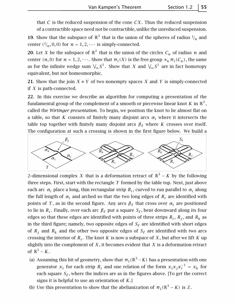
Van Kampen’s Theorem Section 1.2 55
that C is the reduced suspension of the cone CX . Thus the reduced suspension
of a contractible space need not be contractible, unlike the unreduced suspension.
19. Show that the subspace of R3 that is the union of the spheres of radius 1/n and
center (1/n,0,0) for n = 1,2, ··· is simply-connected.
20. Let X be the subspace of R2 that is the union of the circles Cn of radius n and
center (n,0) for n = 1,2, ··· . Show that π1(X) is the free group ∗nπ1(Cn) , the same
as for the infinite wedge sum∨∞S
1 . Show that X and∨∞S
1 are in fact homotopy
equivalent, but not homeomorphic.
21. Show that the join X ∗ Y of two nonempty spaces X and Y is simply-connected
if X is path-connected.
22. In this exercise we describe an algorithm for computing a presentation of the
fundamental group of the complement of a smooth or piecewise linear knot K in R3 ,
called the Wirtinger presentation. To begin, we position the knot to lie almost flat on
a table, so that K consists of finitely many disjoint arcs αi where it intersects the
table top together with finitely many disjoint arcs βℓ where K crosses over itself.
The configuration at such a crossing is shown in the first figure below. We build a
2 dimensional complex X that is a deformation retract of R3− K by the following
three steps. First, start with the rectangle T formed by the table top. Next, just above
each arc αi place a long, thin rectangular strip Ri , curved to run parallel to αi along
the full length of αi and arched so that the two long edges of Ri are identified with
points of T , as in the second figure. Any arcs βℓ that cross over αi are positioned
to lie in Ri . Finally, over each arc βℓ put a square Sℓ , bent downward along its four
edges so that these edges are identified with points of three strips Ri , Rj , and Rk as
in the third figure; namely, two opposite edges of Sℓ are identified with short edges
of Rj and Rk and the other two opposite edges of Sℓ are identified with two arcs
crossing the interior of Ri . The knot K is now a subspace of X , but after we lift K up
slightly into the complement of X , it becomes evident that X is a deformation retract
of R3−K .
(a) Assuming this bit of geometry, show that π1(R3−K) has a presentation with one
generator xi for each strip Ri and one relation of the form xixjx−1i = xk for
each square Sℓ , where the indices are as in the figures above. [To get the correct
signs it is helpful to use an orientation of K .]
(b) Use this presentation to show that the abelianization of π1(R3− K) is Z .

56 Chapter 1 The Fundamental Group
We come now to the second main topic of this chapter, covering spaces. We
have already encountered these briefly in our calculation of π1(S1) which used the
example of the projection R→S1 of a helix onto a circle. As we will see, covering
spaces can be used to calculate fundamental groups of other spaces as well. But the
connection between the fundamental group and covering spaces runs much deeper
than this, and in many ways they can be regarded as two viewpoints toward the same
thing. Algebraic aspects of the fundamental group can often be translated into the
geometric language of covering spaces. This is exemplified in one of the main results
in this section, an exact correspondence between connected covering spaces of a given
space X and subgroups of π1(X) . This is strikingly reminiscent of Galois theory, with
its correspondence between field extensions and subgroups of the Galois group.
Let us recall the definition. A covering space of a space X is a space X together
with a map p : X→X satisfying the following condition: Each point x ∈ X has an
open neighborhood U in X such that p−1(U) is a union of disjoint open sets in X ,
each of which is mapped homeomorphically onto U by p . Such a U is called evenly
covered and the disjoint open sets in X that project homeomorphically to U by p
are called sheets of X over U . If U is connected these sheets are the connected
components of p−1(U) so in this case they are uniquely determined by U , but when
U is not connected the decomposition of p−1(U) into sheets may not be unique. We
allow p−1(U) to be empty, the union of an empty collection of sheets over U , so p
need not be surjective. The number of sheets over U is the cardinality of p−1(x) for
x ∈ U . As x varies over X this number is locally constant, so it is constant if X is
connected.
An example related to the helix example is the helicoid surface S ⊂ R3 consisting
of points of the form (s cos 2πt, s sin 2πt, t) for (s, t) ∈ (0,∞)×R . This projects
onto R2− {0} via the map (x,y, z)֏ (x,y) , and this projection defines a covering
space p :S→R2−{0} since each point of R2
−{0} is contained in an open disk U in
R2−{0} with p−1(U) consisting of countably many disjoint open disks in S projecting
homeomorphically onto U .
Another example is the map p :S1→S1 , p(z) = zn where we
view z as a complex number with |z| = 1 and n is any positive
integer. The closest one can come to realizing this covering space
as a linear projection in 3 space analogous to the projection of the
helix is to draw a circle wrapping around a cylinder n times and
intersecting itself in n − 1 points that one has to imagine are not
really intersections. For an alternative picture without this defect,
embed S1 in the boundary torus of a solid torus S1×D2 so that it winds n times
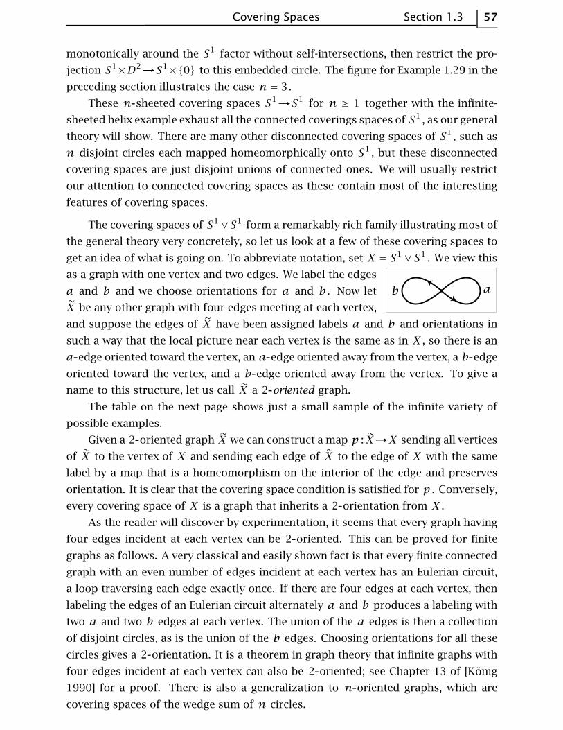
Covering Spaces Section 1.3 57
monotonically around the S1 factor without self-intersections, then restrict the pro-
jection S1×D2→S1
×{0} to this embedded circle. The figure for Example 1.29 in the
preceding section illustrates the case n = 3.
These n sheeted covering spaces S1→S1 for n ≥ 1 together with the infinite-
sheeted helix example exhaust all the connected coverings spaces of S1 , as our general
theory will show. There are many other disconnected covering spaces of S1 , such as
n disjoint circles each mapped homeomorphically onto S1 , but these disconnected
covering spaces are just disjoint unions of connected ones. We will usually restrict
our attention to connected covering spaces as these contain most of the interesting
features of covering spaces.
The covering spaces of S1∨S1 form a remarkably rich family illustrating most of
the general theory very concretely, so let us look at a few of these covering spaces to
get an idea of what is going on. To abbreviate notation, set X = S1∨ S1 . We view this
as a graph with one vertex and two edges. We label the edges
a and b and we choose orientations for a and b . Now let
X be any other graph with four edges meeting at each vertex,
and suppose the edges of X have been assigned labels a and b and orientations in
such a way that the local picture near each vertex is the same as in X , so there is an
a edge oriented toward the vertex, an a edge oriented away from the vertex, a b edge
oriented toward the vertex, and a b edge oriented away from the vertex. To give a
name to this structure, let us call X a 2 oriented graph.
The table on the next page shows just a small sample of the infinite variety of
possible examples.
Given a 2 oriented graph X we can construct a map p : X→X sending all vertices
of X to the vertex of X and sending each edge of X to the edge of X with the same
label by a map that is a homeomorphism on the interior of the edge and preserves
orientation. It is clear that the covering space condition is satisfied for p . Conversely,
every covering space of X is a graph that inherits a 2 orientation from X .
As the reader will discover by experimentation, it seems that every graph having
four edges incident at each vertex can be 2 oriented. This can be proved for finite
graphs as follows. A very classical and easily shown fact is that every finite connected
graph with an even number of edges incident at each vertex has an Eulerian circuit,
a loop traversing each edge exactly once. If there are four edges at each vertex, then
labeling the edges of an Eulerian circuit alternately a and b produces a labeling with
two a and two b edges at each vertex. The union of the a edges is then a collection
of disjoint circles, as is the union of the b edges. Choosing orientations for all these
circles gives a 2 orientation. It is a theorem in graph theory that infinite graphs with
four edges incident at each vertex can also be 2 oriented; see Chapter 13 of [Konig
1990] for a proof. There is also a generalization to n oriented graphs, which are
covering spaces of the wedge sum of n circles.

58 Chapter 1 The Fundamental Group
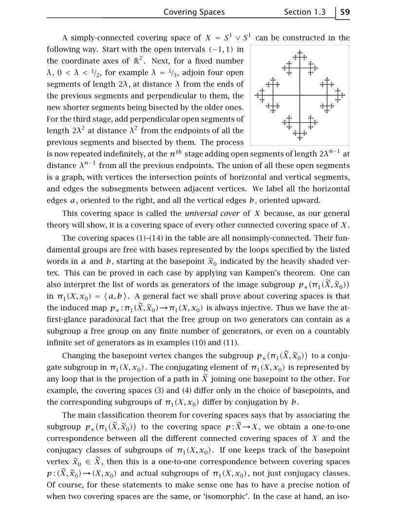
Covering Spaces Section 1.3 59
A simply-connected covering space of X = S1∨ S1 can be constructed in the
following way. Start with the open intervals (−1,1) in
the coordinate axes of R2 . Next, for a fixed number
λ , 0 < λ < 1/2, for example λ = 1/3, adjoin four open
segments of length 2λ , at distance λ from the ends of
the previous segments and perpendicular to them, the
new shorter segments being bisected by the older ones.
For the third stage, add perpendicular open segments of
length 2λ2 at distance λ2 from the endpoints of all the
previous segments and bisected by them. The process
is now repeated indefinitely, at the nth stage adding open segments of length 2λn−1 at
distance λn−1 from all the previous endpoints. The union of all these open segments
is a graph, with vertices the intersection points of horizontal and vertical segments,
and edges the subsegments between adjacent vertices. We label all the horizontal
edges a , oriented to the right, and all the vertical edges b , oriented upward.
This covering space is called the universal cover of X because, as our general
theory will show, it is a covering space of every other connected covering space of X .
The covering spaces (1)–(14) in the table are all nonsimply-connected. Their fun-
damental groups are free with bases represented by the loops specified by the listed
words in a and b , starting at the basepoint x0 indicated by the heavily shaded ver-
tex. This can be proved in each case by applying van Kampen’s theorem. One can
also interpret the list of words as generators of the image subgroup p∗(π1(X, x0)
)
in π1(X,x0) =⟨a,b
⟩. A general fact we shall prove about covering spaces is that
the induced map p∗ :π1(X, x0)→π1(X,x0) is always injective. Thus we have the at-
first-glance paradoxical fact that the free group on two generators can contain as a
subgroup a free group on any finite number of generators, or even on a countably
infinite set of generators as in examples (10) and (11).
Changing the basepoint vertex changes the subgroup p∗(π1(X, x0)
)to a conju-
gate subgroup in π1(X,x0) . The conjugating element of π1(X,x0) is represented by
any loop that is the projection of a path in X joining one basepoint to the other. For
example, the covering spaces (3) and (4) differ only in the choice of basepoints, and
the corresponding subgroups of π1(X,x0) differ by conjugation by b .
The main classification theorem for covering spaces says that by associating the
subgroup p∗(π1(X, x0)
)to the covering space p : X→X , we obtain a one-to-one
correspondence between all the different connected covering spaces of X and the
conjugacy classes of subgroups of π1(X,x0) . If one keeps track of the basepoint
vertex x0 ∈ X , then this is a one-to-one correspondence between covering spaces
p : (X, x0)→(X,x0) and actual subgroups of π1(X,x0) , not just conjugacy classes.
Of course, for these statements to make sense one has to have a precise notion of
when two covering spaces are the same, or ‘isomorphic’. In the case at hand, an iso-

60 Chapter 1 The Fundamental Group
morphism between covering spaces of X is just a graph isomorphism that preserves
the labeling and orientations of edges. Thus the covering spaces in (3) and (4) are
isomorphic, but not by an isomorphism preserving basepoints, so the two subgroups
of π1(X,x0) corresponding to these covering spaces are distinct but conjugate. On
the other hand, the two covering spaces in (5) and (6) are not isomorphic, though the
graphs are homeomorphic, so the corresponding subgroups of π1(X,x0) are isomor-
phic but not conjugate.
Some of the covering spaces (1)–(14) are more symmetric than others, where by
a ‘symmetry’ we mean an automorphism of the graph preserving the labeling and
orientations. The most symmetric covering spaces are those having symmetries taking
any one vertex onto any other. The examples (1), (2), (5)–(8), and (11) are the ones with
this property. We shall see that a covering space of X has maximal symmetry exactly
when the corresponding subgroup of π1(X,x0) is a normal subgroup, and in this case
the symmetries form a group isomorphic to the quotient group of π1(X,x0) by the
normal subgroup. Since every group generated by two elements is a quotient group
of Z∗ Z , this implies that every two-generator group is the symmetry group of some
covering space of X .
Lifting Properties
Covering spaces are defined in fairly geometric terms, as maps p : X→X that are
local homeomorphisms in a rather strong sense. But from the viewpoint of algebraic
topology, the distinctive feature of covering spaces is their behavior with respect to
lifting of maps. Recall the terminology from the proof of Theorem 1.7: A lift of a map
f :Y→X is a map f :Y→X such that pf = f . We will describe three special lifting
properties of covering spaces and derive a few applications of these.
First we have the homotopy lifting property, also known as the covering homo-
topy property:
Proposition 1.30. Given a covering space p : X→X , a homotopy ft :Y→X , and a
map f0 :Y→X lifting f0 , then there exists a unique homotopy ft :Y→X of f0 that
lifts ft .
Proof: This was proved as property (c) in the proof of Theorem 1.7. ⊔⊓
Taking Y to be a point gives the path lifting property for a covering space
p : X→X , which says that for each path f : I→X and each lift x0 of the starting
point f(0) = x0 there is a unique path f : I→X lifting f starting at x0 . In particular,
the uniqueness of lifts implies that every lift of a constant path is constant, but this
could be deduced more simply from the fact that p−1(x0) has the discrete topology,
by the definition of a covering space.

Covering Spaces Section 1.3 61
Taking Y to be I , we see that every homotopy ft of a path f0 in X lifts to a
homotopy ft of each lift f0 of f0 . The lifted homotopy ft is a homotopy of paths,
fixing the endpoints, since as t varies each endpoint of ft traces out a path lifting a
constant path, which must therefore be constant.
Here is a simple application:
Proposition 1.31. The map p∗ :π1(X, x0)→π1(X,x0) induced by a covering space
p : (X, x0)→(X,x0) is injective. The image subgroup p∗(π1(X, x0)
)in π1(X,x0)
consists of the homotopy classes of loops in X based at x0 whose lifts to X starting
at x0 are loops.
Proof: An element of the kernel of p∗ is represented by a loop f0 : I→X with a
homotopy ft : I→X of f0 = pf0 to the trivial loop f1 . By the remarks preceding the
proposition, there is a lifted homotopy of loops ft starting with f0 and ending with
a constant loop. Hence [f0] = 0 in π1(X, x0) and p∗ is injective.
For the second statement of the proposition, loops at x0 lifting to loops at x0
certainly represent elements of the image of p∗ :π1(X, x0)→π1(X,x0) . Conversely,
a loop representing an element of the image of p∗ is homotopic to a loop having such
a lift, so by homotopy lifting, the loop itself must have such a lift. ⊔⊓
Proposition 1.32. The number of sheets of a covering space p : (X, x0)→(X,x0)
with X and X path-connected equals the index of p∗(π1(X, x0)
)in π1(X,x0) .
Proof: For a loop g in X based at x0 , let g be its lift to X starting at x0 . A product
h g with [h] ∈ H = p∗(π1(X, x0)
)has the lift h g ending at the same point as g
since h is a loop. Thus we may define a function Φ from cosets H[g] to p−1(x0)
by sending H[g] to g(1) . The path-connectedness of X implies that Φ is surjective
since x0 can be joined to any point in p−1(x0) by a path g projecting to a loop g at
x0 . To see that Φ is injective, observe that Φ(H[g1]) = Φ(H[g2]) implies that g1 g2
lifts to a loop in X based at x0 , so [g1][g2]−1∈ H and hence H[g1] = H[g2] . ⊔⊓
It is important also to know about the existence and uniqueness of lifts of general
maps, not just lifts of homotopies. For the existence question an answer is provided
by the following lifting criterion:
Proposition 1.33. Suppose given a covering space p : (X, x0)→(X,x0) and a map
f : (Y ,y0)→(X,x0) with Y path-connected and locally path-connected. Then a lift
f : (Y ,y0)→(X, x0) of f exists iff f∗(π1(Y ,y0)
)⊂ p∗
(π1(X, x0)
).
When we say a space has a certain property locally, such as being locally path-
connected, we usually mean that each point has arbitrarily small open neighborhoods
with this property. Thus for Y to be locally path-connected means that for each point
y ∈ Y and each neighborhood U of y there is an open neighborhood V ⊂ U of
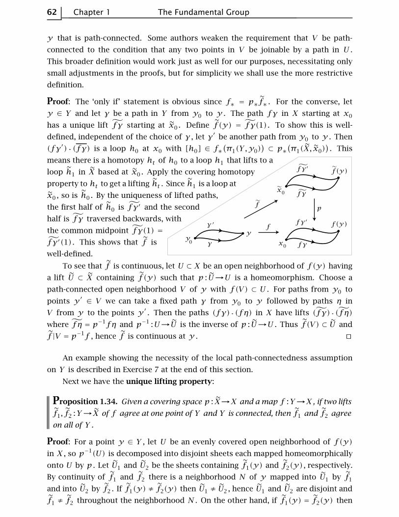
62 Chapter 1 The Fundamental Group
y that is path-connected. Some authors weaken the requirement that V be path-
connected to the condition that any two points in V be joinable by a path in U .
This broader definition would work just as well for our purposes, necessitating only
small adjustments in the proofs, but for simplicity we shall use the more restrictive
definition.
Proof: The ‘only if’ statement is obvious since f∗ = p∗f∗ . For the converse, let
y ∈ Y and let γ be a path in Y from y0 to y . The path fγ in X starting at x0
has a unique lift f γ starting at x0 . Define f (y) = f γ(1) . To show this is well-
defined, independent of the choice of γ , let γ′ be another path from y0 to y . Then
(fγ′) (fγ) is a loop h0 at x0 with [h0] ∈ f∗(π1(Y ,y0)
)⊂ p∗
(π1(X, x0)
). This
means there is a homotopy ht of h0 to a loop h1 that lifts to a
loop h1 in X based at x0 . Apply the covering homotopy
property to ht to get a lifting ht . Since h1 is a loop at
x0 , so is h0 . By the uniqueness of lifted paths,
the first half of h0 is f γ′ and the second
half is f γ traversed backwards, with
the common midpoint f γ(1) =
f γ′(1) . This shows that f is
well-defined.
To see that f is continuous, let U ⊂ X be an open neighborhood of f(y) having
a lift U ⊂ X containing f (y) such that p : U→U is a homeomorphism. Choose a
path-connected open neighborhood V of y with f(V) ⊂ U . For paths from y0 to
points y ′ ∈ V we can take a fixed path γ from y0 to y followed by paths η in
V from y to the points y ′ . Then the paths (fγ) (fη) in X have lifts (fγ) (fη)
where f η = p−1fη and p−1 :U→U is the inverse of p : U→U . Thus f (V) ⊂ U and
f |V = p−1f , hence f is continuous at y . ⊔⊓
An example showing the necessity of the local path-connectedness assumption
on Y is described in Exercise 7 at the end of this section.
Next we have the unique lifting property:
Proposition 1.34. Given a covering space p : X→X and a map f :Y→X , if two lifts
f1, f2 :Y→X of f agree at one point of Y and Y is connected, then f1 and f2 agree
on all of Y .
Proof: For a point y ∈ Y , let U be an evenly covered open neighborhood of f(y)
in X , so p−1(U) is decomposed into disjoint sheets each mapped homeomorphically
onto U by p . Let U1 and U2 be the sheets containing f1(y) and f2(y) , respectively.
By continuity of f1 and f2 there is a neighborhood N of y mapped into U1 by f1
and into U2 by f2 . If f1(y) ≠ f2(y) then U1 ≠ U2 , hence U1 and U2 are disjoint and
f1 ≠ f2 throughout the neighborhood N . On the other hand, if f1(y) = f2(y) then

Covering Spaces Section 1.3 63
U1 = U2 so f1 = f2 on N since pf1 = pf2 and p is injective on U1 = U2 . Thus the
set of points where f1 and f2 agree is both open and closed in Y . ⊔⊓
The Classification of Covering Spaces
We consider next the problem of classifying all the different covering spaces of
a fixed space X . Since the whole chapter is about paths, it should not be surprising
that we will restrict attention to spaces X that are at least locally path-connected.
Path-components of X are then the same as components, and for the purpose of
classifying the covering spaces of X there is no loss in assuming that X is connected,
or equivalently, path-connected. Local path-connectedness is inherited by covering
spaces, so these too are connected iff they are path-connected. The main thrust of the
classification will be the Galois correspondence between connected covering spaces of
X and subgroups of π1(X) , but when this is finished we will also describe a different
method of classification that includes disconnected covering spaces as well.
The Galois correspondence arises from the function that assigns to each covering
space p : (X, x0)→(X,x0) the subgroup p∗(π1(X, x0)
)of π1(X,x0) . First we con-
sider whether this function is surjective. That is, we ask whether every subgroup of
π1(X,x0) is realized as p∗(π1(X, x0)
)for some covering space p : (X, x0)→(X,x0) .
In particular we can ask whether the trivial subgroup is realized. Since p∗ is always
injective, this amounts to asking whether X has a simply-connected covering space.
Answering this will take some work.
A necessary condition for X to have a simply-connected covering space is the
following: Each point x ∈ X has a neighborhood U such that the inclusion-induced
map π1(U,x)→π1(X,x) is trivial; one says X is semilocally simply-connected if
this holds. To see the necessity of this condition, suppose p : X→X is a covering
space with X simply-connected. Every point x ∈ X has a neighborhood U having a
lift U ⊂ X projecting homeomorphically to U by p . Each loop in U lifts to a loop
in U , and the lifted loop is nullhomotopic in X since π1(X) = 0. So, composing this
nullhomotopy with p , the original loop in U is nullhomotopic in X .
A locally simply-connected space is certainly semilocally simply-connected. For
example, CW complexes have the much stronger property of being locally contractible,
as we show in the Appendix. An example of a space that is not semilocally simply-
connected is the shrinking wedge of circles, the subspace X ⊂ R2 consisting of the
circles of radius 1/n centered at the point (1/n,0) for n = 1,2, ··· , introduced in Exam-
ple 1.25. On the other hand, the cone CX = (X×I)/(X×{0}) is semilocally simply-
connected since it is contractible, but it is not locally simply-connected.
We shall now show how to construct a simply-connected covering space of X if
X is path-connected, locally path-connected, and semilocally simply-connected. To
motivate the construction, suppose p : (X, x0)→(X,x0) is a simply-connected cover-
ing space. Each point x ∈ X can then be joined to x0 by a unique homotopy class of
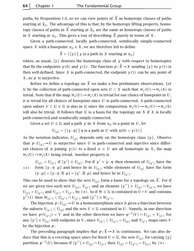
64 Chapter 1 The Fundamental Group
paths, by Proposition 1.6, so we can view points of X as homotopy classes of paths
starting at x0 . The advantage of this is that, by the homotopy lifting property, homo-
topy classes of paths in X starting at x0 are the same as homotopy classes of paths
in X starting at x0 . This gives a way of describing X purely in terms of X .
Given a path-connected, locally path-connected, semilocally simply-connected
space X with a basepoint x0 ∈ X , we are therefore led to define
X ={[γ] |||| γ is a path in X starting at x0
}
where, as usual, [γ] denotes the homotopy class of γ with respect to homotopies
that fix the endpoints γ(0) and γ(1) . The function p : X→X sending [γ] to γ(1) is
then well-defined. Since X is path-connected, the endpoint γ(1) can be any point of
X , so p is surjective.
Before we define a topology on X we make a few preliminary observations. Let
U be the collection of path-connected open sets U ⊂ X such that π1(U)→π1(X) is
trivial. Note that if the map π1(U)→π1(X) is trivial for one choice of basepoint in U ,
it is trivial for all choices of basepoint since U is path-connected. A path-connected
open subset V ⊂ U ∈ U is also in U since the composition π1(V)→π1(U)→π1(X)
will also be trivial. It follows that U is a basis for the topology on X if X is locally
path-connected and semilocally simply-connected.
Given a set U ∈ U and a path γ in X from x0 to a point in U , let
U[γ] ={[γ η] |||| η is a path in U with η(0) = γ(1)
}
As the notation indicates, U[γ] depends only on the homotopy class [γ] . Observe
that p :U[γ]→U is surjective since U is path-connected and injective since differ-
ent choices of η joining γ(1) to a fixed x ∈ U are all homotopic in X , the map
π1(U)→π1(X) being trivial. Another property is
(∗)
U[γ] = U[γ′] if [γ′] ∈ U[γ] . For if γ′ = γ η then elements of U[γ′] have the
form [γ η µ] and hence lie in U[γ] , while elements of U[γ] have the form
[γ µ] = [γ η η µ] = [γ′ η µ] and hence lie in U[γ′] .
This can be used to show that the sets U[γ] form a basis for a topology on X . For if
we are given two such sets U[γ] , V[γ′] and an element [γ′′] ∈ U[γ] ∩ V[γ′] , we have
U[γ] = U[γ′′] and V[γ′] = V[γ′′] by (∗) . So if W ∈ U is contained in U∩V and contains
γ′′(1) then W[γ′′] ⊂ U[γ′′] ∩ V[γ′′] and [γ′′] ∈ W[γ′′] .
The bijection p :U[γ]→U is a homeomorphism since it gives a bijection between
the subsets V[γ′] ⊂ U[γ] and the sets V ∈ U contained in U . Namely, in one direction
we have p(V[γ′]) = V and in the other direction we have p−1(V) ∩ U[γ] = V[γ′] for
any [γ′] ∈ U[γ] with endpoint in V , since V[γ′] ⊂ U[γ′] = U[γ] and V[γ′] maps onto V
by the bijection p .
The preceding paragraph implies that p : X→X is continuous. We can also de-
duce that this is a covering space since for fixed U ∈ U , the sets U[γ] for varying [γ]
partition p−1(U) because if [γ′′] ∈ U[γ] ∩U[γ′] then U[γ] = U[γ′′] = U[γ′] by (∗) .

Covering Spaces Section 1.3 65
It remains only to show that X is simply-connected. For a point [γ] ∈ X let γtbe the path in X that equals γ on [0, t] and is stationary at γ(t) on [t,1] . Then the
function t֏ [γt] is a path in X lifting γ that starts at [x0] , the homotopy class of
the constant path at x0 , and ends at [γ] . Since [γ] was an arbitrary point in X , this
shows that X is path-connected. To show that π1(X, [x0]) = 0 it suffices to show
that the image of this group under p∗ is trivial since p∗ is injective. Elements in the
image of p∗ are represented by loops γ at x0 that lift to loops in X at [x0] . We have
observed that the path t֏ [γt] lifts γ starting at [x0] , and for this lifted path to
be a loop means that [γ1] = [x0] . Since γ1 = γ , this says that [γ] = [x0] , so γ is
nullhomotopic and the image of p∗ is trivial.
This completes the construction of a simply-connected covering space X→X .
In concrete cases one usually constructs a simply-connected covering space by
more direct methods. For example, suppose X is the union of subspaces A and B for
which simply-connected covering spaces A→A and B→B are already known. Then
one can attempt to build a simply-connected covering space X→X by assembling
copies of A and B . For example, for X = S1∨ S1 , if we take A and B to be the two
circles, then A and B are each R , and we can build the simply-connected cover X
described earlier in this section by glueing together infinitely many copies of A and
B , the horizontal and vertical lines in X . Here is another illustration of this method:
Example 1.35. For integers m,n ≥ 2, let Xm,n be the quotient space of a cylinder
S1×I under the identifications (z,0) ∼ (e2πi/mz,0) and (z,1) ∼ (e2πi/nz,1) . Let
A ⊂ X and B ⊂ X be the quotients of S1×[0, 1/2] and S1
×[1/2,1], so A and B are
the mapping cylinders of z֏ zm and z֏ zn , with A∩ B = S1 . The simplest case
is m = n = 2, when A and B are Mobius bands and X2,2 is the Klein bottle. We
encountered the complexes Xm,n previously in analyzing torus knot complements in
Example 1.24.
The figure for Example 1.29 at the end of the preceding section
shows what A looks like in the typical case m = 3. We have π1(A) ≈ Z ,
and the universal cover A is homeomorphic to a product Cm×R where
Cm is the graph that is a cone on m points, as shown in the figure to
the right. The situation for B is similar, and B is homeomorphic to
Cn×R . Now we attempt to build the universal cover Xm,n from copies
of A and B . Start with a copy of A . Its boundary, the outer edges of
its fins, consists of m copies of R . Along each of these m boundary
lines we attach a copy of B . Each of these copies of B has one of its boundary lines
attached to the initial copy of A , leaving n− 1 boundary lines free, and we attach a
new copy of A to each of these free boundary lines. Thus we now have m(n− 1)+ 1
copies of A . Each of the newly attached copies of A has m − 1 free boundary lines,
and to each of these lines we attach a new copy of B . The process is now repeated ad

66 Chapter 1 The Fundamental Group
infinitum in the evident way. Let Xm,n be the resulting space.
The product structures A = Cm×R and B = Cn×R
give Xm,n the structure of a product Tm,n×R where Tm,nis an infinite graph constructed by an inductive scheme
just like the construction of Xm,n . Thus Tm,n is the union
of a sequence of finite subgraphs, each obtained from the
preceding by attaching new copies of Cm or Cn . Each
of these finite subgraphs deformation retracts onto the
preceding one. The infinite concatenation of these defor-
mation retractions, with the kth graph deformation retracting to the previous one
during the time interval [1/2k,1/2k−1] , gives a deformation retraction of Tm,n onto
the initial stage Cm . Since Cm is contractible, this means Tm,n is contractible, hence
also Xm,n , which is the product Tm,n×R . In particular, Xm,n is simply-connected.
The map that projects each copy of A in Xm,n to A and
each copy of B to B is a covering space. To define this map
precisely, choose a point x0 ∈ S1 , and then the image of the
line segment {x0}× I in Xm,n meets A in a line segment whose
preimage in A consists of an infinite number of line segments,
appearing in the earlier figure as the horizontal segments spi-
raling around the central vertical axis. The picture in B is
similar, and when we glue together all the copies of A and B
to form Xm,n , we do so in such a way that these horizontal segments always line up
exactly. This decomposes Xm,n into infinitely many rectangles, each formed from a
rectangle in an A and a rectangle in a B . The covering projection Xm,n→Xm,n is the
quotient map that identifies all these rectangles.
Now we return to the general theory. The hypotheses for constructing a simply-
connected covering space of X in fact suffice for constructing covering spaces realiz-
ing arbitrary subgroups of π1(X) :
Proposition 1.36. Suppose X is path-connected, locally path-connected, and semilo-
cally simply-connected. Then for every subgroup H ⊂ π1(X,x0) there is a covering
space p :XH→X such that p∗(π1(XH , x0)
)= H for a suitably chosen basepoint
x0 ∈ XH .
Proof: For points [γ] , [γ′] in the simply-connected covering space X constructed
above, define [γ] ∼ [γ′] to mean γ(1) = γ′(1) and [γ γ′] ∈ H . It is easy to see that
this is an equivalence relation since H is a subgroup: it is reflexive since H contains
the identity element, symmetric since H is closed under inverses, and transitive since
H is closed under multiplication. Let XH be the quotient space of X obtained by
identifying [γ] with [γ′] if [γ] ∼ [γ′] . Note that if γ(1) = γ′(1) , then [γ] ∼ [γ′]
iff [γ η] ∼ [γ′ η] . This means that if any two points in basic neighborhoods U[γ]
Covering Spaces Section 1.3 67
and U[γ′] are identified in XH then the whole neighborhoods are identified. Hence
the natural projection XH→X induced by [γ]֏ γ(1) is a covering space.
If we choose for the basepoint x0 ∈ XH the equivalence class of the constant path
c at x0 , then the image of p∗ :π1(XH , x0)→π1(X,x0) is exactly H . This is because
for a loop γ in X based at x0 , its lift to X starting at [c] ends at [γ] , so the image
of this lifted path in XH is a loop iff [γ] ∼ [c] , or equivalently, [γ] ∈ H . ⊔⊓
Having taken care of the existence of covering spaces of X corresponding to all
subgroups of π1(X) , we turn now to the question of uniqueness. More specifically,
we are interested in uniqueness up to isomorphism, where an isomorphism between
covering spaces p1 : X1→X and p2 : X2→X is a homeomorphism f : X1→X2 such
that p1 = p2f . This condition means exactly that f preserves the covering space
structures, taking p−11 (x) to p−1
2 (x) for each x ∈ X . The inverse f−1 is then also an
isomorphism, and the composition of two isomorphisms is an isomorphism, so we
have an equivalence relation.
Proposition 1.37. If X is path-connected and locally path-connected, then two path-
connected covering spaces p1 : X1→X and p2 : X2→X are isomorphic via an isomor-
phism f : X1→X2 taking a basepoint x1 ∈ p−11 (x0) to a basepoint x2 ∈ p
−12 (x0) iff
p1∗
(π1(X1, x1)
)= p2∗
(π1(X2, x2)
).
Proof: If there is an isomorphism f : (X1, x1)→(X2, x2) , then from the two relations
p1 = p2f and p2 = p1f−1 it follows that p1∗
(π1(X1, x1)
)= p2∗
(π1(X2, x2)
). Con-
versely, suppose that p1∗
(π1(X1, x1)
)= p2∗
(π1(X2, x2)
). By the lifting criterion,
we may lift p1 to a map p1 : (X1, x1)→(X2, x2) with p2p1 = p1 . Symmetrically, we
obtain p2 : (X2, x2)→(X1, x1) with p1p2 = p2 . Then by the unique lifting property,
p1p2 = 11 and p2p1 = 11 since these composed lifts fix the basepoints. Thus p1 and
p2 are inverse isomorphisms. ⊔⊓
We have proved the first half of the following classification theorem:
Theorem 1.38. Let X be path-connected, locally path-connected, and semilocally
simply-connected. Then there is a bijection between the set of basepoint-preserving
isomorphism classes of path-connected covering spaces p : (X, x0)→(X,x0) and the
set of subgroups of π1(X,x0) , obtained by associating the subgroup p∗(π1(X, x0)
)
to the covering space (X, x0) . If basepoints are ignored, this correspondence gives a
bijection between isomorphism classes of path-connected covering spaces p : X→Xand conjugacy classes of subgroups of π1(X,x0) .
Proof: It remains only to prove the last statement. We show that for a covering space
p : (X, x0)→(X,x0) , changing the basepoint x0 within p−1(x0) corresponds exactly
to changing p∗(π1(X, x0)
)to a conjugate subgroup of π1(X,x0) . Suppose that x1
is another basepoint in p−1(x0) , and let γ be a path from x0 to x1 . Then γ projects

68 Chapter 1 The Fundamental Group
to a loop γ in X representing some element g ∈ π1(X,x0) . Set Hi = p∗(π1(X, xi)
)
for i = 0,1. We have an inclusion g−1H0g ⊂ H1 since for f a loop at x0 , γ f γ is
a loop at x1 . Similarly we have gH1g−1⊂ H0 . Conjugating the latter relation by g−1
gives H1 ⊂ g−1H0g , so g−1H0g = H1 . Thus, changing the basepoint from x0 to x1
changes H0 to the conjugate subgroup H1 = g−1H0g .
Conversely, to change H0 to a conjugate subgroup H1 = g−1H0g , choose a loop
γ representing g , lift this to a path γ starting at x0 , and let x1 = γ(1) . The preceding
argument then shows that we have the desired relation H1 = g−1H0g . ⊔⊓
A consequence of the lifting criterion is that a simply-connected covering space of
a path-connected, locally path-connected space X is a covering space of every other
path-connected covering space of X . A simply-connected covering space of X is
therefore called a universal cover. It is unique up to isomorphism, so one is justified
in calling it the universal cover.
More generally, there is a partial ordering on the various path-connected covering
spaces of X , according to which ones cover which others. This corresponds to the
partial ordering by inclusion of the corresponding subgroups of π1(X) , or conjugacy
classes of subgroups if basepoints are ignored.
Representing Covering Spaces by Permutations
We wish to describe now another way of classifying the different covering spaces
of a connected, locally path-connected, semilocally simply-connected space X , with-
out restricting just to connected covering spaces. To give the idea, con-
sider the 3 sheeted covering spaces of S1 . There are three of these,
X1 , X2 , and X3 , with the subscript indicating the number of compo-
nents. For each of these covering spaces p : Xi→S1 the three different
lifts of a loop in S1 generating π1(S1, x0) determine a permutation of
p−1(x0) sending the starting point of the lift to the ending point of the
lift. For X1 this is a cyclic permutation, for X2 it is a transposition of
two points fixing the third point, and for X3 it is the identity permu-
tation. These permutations obviously determine the covering spaces
uniquely, up to isomorphism. The same would be true for n sheeted
covering spaces of S1 for arbitrary n , even for n infinite.
The covering spaces of S1∨ S1 can be encoded using the same idea. Referring
back to the large table of examples near the beginning of this section, we see in the
covering space (1) that the loop a lifts to the identity permutation of the two vertices
and b lifts to the permutation that transposes the two vertices. In (2), both a and b
lift to transpositions of the two vertices. In (3) and (4), a and b lift to transpositions of
different pairs of the three vertices, while in (5) and (6) they lift to cyclic permutations
of the vertices. In (11) the vertices can be labeled by Z , with a lifting to the identity
permutation and b lifting to the shift n֏ n + 1. Indeed, one can see from these

Covering Spaces Section 1.3 69
examples that a covering space of S1∨ S1 is nothing more than an efficient graphical
representation of a pair of permutations of a given set.
This idea of lifting loops to permutations generalizes to arbitrary covering spaces.
For a covering space p : X→X , a path γ in X has a unique lift γ starting at a given
point of p−1(γ(0)) , so we obtain a well-defined map Lγ :p−1(γ(0))→p−1(γ(1)) by
sending the starting point γ(0) of each lift γ to its ending point γ(1) . It is evident
that Lγ is a bijection since Lγ is its inverse. For a composition of paths γ η we have
Lγ·η = LηLγ , rather than LγLη , since composition of paths is written from left to
right while composition of functions is written from right to left. To compensate for
this, let us modify the definition by replacing Lγ by its inverse. Thus the new Lγ is
a bijection p−1(γ(1))→p−1(γ(0)) , and Lγ·η = LγLη . Since Lγ depends only on the
homotopy class of γ , this means that if we restrict attention to loops at a basepoint
x0 ∈ X , then the association γ֏ Lγ gives a homomorphism from π1(X,x0) to the
group of permutations of p−1(x0) . This is called the action of π1(X,x0) on the fiber
p−1(x0) .
Let us see how the covering space p : X→X can be reconstructed from the associ-
ated action of π1(X,x0) on the fiber F = p−1(x0) , assuming that X is path-connected,
locally path-connected, and semilocally simply-connected, so it has a universal cover
X0→X . We can take the points of X0 to be homotopy classes of paths in X starting
at x0 , as in the general construction of a universal cover. Define a map h : X0×F→Xsending a pair ([γ], x0) to γ(1) where γ is the lift of γ to X starting at x0 . Then h
is continuous, and in fact a local homeomorphism, since a neighborhood of ([γ], x0)
in X0×F consists of the pairs ([γ η], x0) with η a path in a suitable neighborhood
of γ(1) . It is obvious that h is surjective since X is path-connected. If h were injec-
tive as well, it would be a homeomorphism, which is unlikely since X is probably not
homeomorphic to X0×F . Even if h is not injective, it will induce a homeomorphism
from some quotient space of X0×F onto X . To see what this quotient space is,
suppose h([γ], x0) = h([γ′], x′0) . Then γ and γ′ are both
paths from x0 to the same endpoint, and from the figure
we see that x′0 = Lγ′·γ(x0) . Letting λ be the loop γ′ γ , this
means that h([γ], x0) = h([λ γ], Lλ(x0)) . Conversely, for
any loop λ we have h([γ], x0) = h([λ γ], Lλ(x0)) . Thus h
induces a well-defined map to X from the quotient space of
X0×F obtained by identifying ([γ], x0) with ([λ γ], Lλ(x0))
for each [λ] ∈ π1(X,x0) . Let this quotient space be denoted Xρ where ρ is the ho-
momorphism from π1(X,x0) to the permutation group of F specified by the action.
Notice that the definition of Xρ makes sense whenever we are given an action
ρ of π1(X,x0) on a set F . There is a natural projection Xρ→X sending ([γ], x0)
to γ(1) , and this is a covering space since if U ⊂ X is an open set over which the
universal cover X0 is a product U×π1(X,x0) , then the identifications defining Xρ

70 Chapter 1 The Fundamental Group
simply collapse U×π1(X,x0)×F to U×F .
Returning to our given covering space X→X with associated action ρ , the map
Xρ→X induced by h is a bijection and therefore a homeomorphism since h was a
local homeomorphism. Since this homeomorphism Xρ→X takes each fiber of Xρ to
the corresponding fiber of X , it is an isomorphism of covering spaces.
If two covering spaces p1 : X1→X and p2 : X2→X are isomorphic, one may ask
how the corresponding actions of π1(X,x0) on the fibers F1 and F2 over x0 are
related. An isomorphism h : X1→X2 restricts to a bijection F1→F2 , and evidently
Lγ(h(x0)) = h(Lγ(x0)) . Using the less cumbersome notation γx0 for Lγ(x0) , this
relation can be written more concisely as γh(x0) = h(γx0) . A bijection F1→F2 with
this property is what one would naturally call an isomorphism of sets with π1(X,x0)
action. Thus isomorphic covering spaces have isomorphic actions on fibers. The
converse is also true, and easy to prove. One just observes that for isomorphic actions
ρ1 and ρ2 , an isomorphism h :F1→F2 induces a map Xρ1→Xρ2and h−1 induces a
similar map in the opposite direction, such that the compositions of these two maps,
in either order, are the identity.
This shows that n sheeted covering spaces of X are classified by equivalence
classes of homomorphisms π1(X,x0)→Σn , where Σn is the symmetric group on n
symbols and the equivalence relation identifies a homomorphism ρ with each of its
conjugates h−1ρh by elements h ∈ Σn . The study of the various homomorphisms
from a given group to Σn is a very classical topic in group theory, so we see that this
algebraic question has a nice geometric interpretation.
Deck Transformations and Group Actions
For a covering space p : X→X the isomorphisms X→X are called deck transfor-
mations or covering transformations. These form a group G(X) under composition.
For example, for the covering space p :R→S1 projecting a vertical helix onto a circle,
the deck transformations are the vertical translations taking the helix onto itself, so
G(X) ≈ Z in this case. For the n sheeted covering space S1→S1 , z֏ zn , the deck
transformations are the rotations of S1 through angles that are multiples of 2π/n ,
so G(X) = Zn .
By the unique lifting property, a deck transformation is completely determined
by where it sends a single point, assuming X is path-connected. In particular, only
the identity deck transformation can fix a point of X .
A covering space p : X→X is called normal if for each x ∈ X and each pair of lifts
x, x′ of x there is a deck transformation taking x to x′. For example, the covering
space R→S1 and the n sheeted covering spaces S1→S1 are normal. Intuitively, a
normal covering space is one with maximal symmetry. This can be seen in the covering
spaces of S1∨S1 shown in the table earlier in this section, where the normal covering
Covering Spaces Section 1.3 71
spaces are (1), (2), (5)–(8), and (11). Note that in (7) the group of deck transformations
is Z4 while in (8) it is Z2×Z2 .
Sometimes normal covering spaces are called regular covering spaces. The term
‘normal’ is motivated by the following result.
Proposition 1.39. Let p : (X, x0)→(X,x0) be a path-connected covering space of
the path-connected, locally path-connected space X , and let H be the subgroup
p∗(π1(X, x0)
)⊂ π1(X,x0) . Then :
(a) This covering space is normal iff H is a normal subgroup of π1(X,x0) .
(b) G(X) is isomorphic to the quotient N(H)/H where N(H) is the normalizer of
H in π1(X,x0) .
In particular, G(X) is isomorphic to π1(X,x0)/H if X is a normal covering. Hence
for the universal cover X→X we have G(X) ≈ π1(X) .
Proof: We observed earlier in the proof of the classification theorem that changing
the basepoint x0 ∈ p−1(x0) to x1 ∈ p
−1(x0) corresponds precisely to conjugating
H by an element [γ] ∈ π1(X,x0) where γ lifts to a path γ from x0 to x1 . Thus [γ]
is in the normalizer N(H) iff p∗(π1(X, x0)
)= p∗
(π1(X, x1)
), which by the lifting
criterion is equivalent to the existence of a deck transformation taking x0 to x1 .
Hence the covering space is normal iff N(H) = π1(X,x0) , that is, iff H is a normal
subgroup of π1(X,x0) .
Define ϕ :N(H)→G(X) sending [γ] to the deck transformation τ taking x0 to
x1 , in the notation above. Then ϕ is a homomorphism, for if γ′ is another loop corre-
sponding to the deck transformation τ′ taking x0 to x′1 then γ γ′ lifts to γ (τ(γ′)) ,
a path from x0 to τ(x′1) = ττ′(x0) , so ττ′ is the deck transformation corresponding
to [γ][γ′] . By the preceding paragraph ϕ is surjective. Its kernel consists of classes
[γ] lifting to loops in X . These are exactly the elements of p∗(π1(X, x0)
)= H . ⊔⊓
The group of deck transformations is a special case of the general notion of
‘groups acting on spaces’. Given a group G and a space Y , then an action of G
on Y is a homomorphism ρ from G to the group Homeo(Y ) of all homeomorphisms
from Y to itself. Thus to each g ∈ G is associated a homeomorphism ρ(g) :Y→Y ,
which for notational simplicity we write simply as g :Y→Y . For ρ to be a homo-
morphism amounts to requiring that g1(g2(y)) = (g1g2)(y) for all g1, g2 ∈ G and
y ∈ Y . If ρ is injective then it identifies G with a subgroup of Homeo(Y ) , and in
practice not much is lost in assuming ρ is an inclusion GHomeo(Y ) since in any
case the subgroup ρ(G) ⊂ Homeo(Y ) contains all the topological information about
the action.
72 Chapter 1 The Fundamental Group
We shall be interested in actions satisfying the following condition:
(∗)Each y ∈ Y has a neighborhood U such that all the images g(U) for varying
g ∈ G are disjoint. In other words, g1(U)∩ g2(U) ≠∅ implies g1 = g2 .
The action of the deck transformation group G(X) on X satisfies (∗) . To see this,
let U ⊂ X project homeomorphically to U ⊂ X . If g1(U) ∩ g2(U) ≠ ∅ for some
g1, g2 ∈ G(X) , then g1(x1) = g2(x2) for some x1, x2 ∈ U . Since x1 and x2 must lie
in the same set p−1(x) , which intersects U in only one point, we must have x1 = x2 .
Then g−11 g2 fixes this point, so g−1
1 g2 = 11 and g1 = g2 .
Note that in (∗) it suffices to take g1 to be the identity since g1(U)∩g2(U) ≠∅
is equivalent to U ∩ g−11 g2(U) ≠ ∅ . Thus we have the equivalent condition that
U ∩ g(U) ≠∅ only when g is the identity.
Given an action of a group G on a space Y , we can form a space Y/G , the quotient
space of Y in which each point y is identified with all its images g(y) as g ranges
over G . The points of Y/G are thus the orbits Gy = {g(y) | g ∈ G } in Y , and
Y/G is called the orbit space of the action. For example, for a normal covering space
X→X , the orbit space X/G(X) is just X .
Proposition 1.40. If an action of a group G on a space Y satisfies (∗) , then :
(a) The quotient map p :Y→Y/G , p(y) = Gy , is a normal covering space.
(b) G is the group of deck transformations of this covering space Y→Y/G if Y is
path-connected.
(c) G is isomorphic to π1(Y/G)/p∗(π1(Y )
)if Y is path-connected and locally path-
connected.
Proof: Given an open set U ⊂ Y as in condition (∗) , the quotient map p simply
identifies all the disjoint homeomorphic sets {g(U) | g ∈ G } to a single open set
p(U) in Y/G . By the definition of the quotient topology on Y/G , p restricts to
a homeomorphism from g(U) onto p(U) for each g ∈ G so we have a covering
space. Each element of G acts as a deck transformation, and the covering space is
normal since g2g−11 takes g1(U) to g2(U) . The deck transformation group contains
G as a subgroup, and equals this subgroup if Y is path-connected, since if f is any
deck transformation, then for an arbitrarily chosen point y ∈ Y , y and f(y) are
in the same orbit and there is a g ∈ G with g(y) = f(y) , hence f = g since deck
transformations of a path-connected covering space are uniquely determined by where
they send a point. The final statement of the proposition is immediate from part (b)
of Proposition 1.39. ⊔⊓
In view of the preceding proposition, we shall call an action satisfying (∗) a
covering space action. This is not standard terminology, but there does not seem to
be a universally accepted name for actions satisfying (∗) . Sometimes these are called
‘properly discontinuous’ actions, but more often this rather unattractive term means

Covering Spaces Section 1.3 73
something weaker: Every point x ∈ X has a neighborhood U such that U ∩ g(U)
is nonempty for only finitely many g ∈ G . Many symmetry groups have this proper
discontinuity property without satisfying (∗) , for example the group of symmetries
of the familiar tiling of R2 by regular hexagons. The reason why the action of this
group on R2 fails to satisfy (∗) is that there are fixed points: points y for which
there is a nontrivial element g ∈ G with g(y) = y . For example, the vertices of the
hexagons are fixed by the 120 degree rotations about these points, and the midpoints
of edges are fixed by 180 degree rotations. An action without fixed points is called a
free action. Thus for a free action of G on Y , only the identity element of G fixes any
point of Y . This is equivalent to requiring that all the images g(y) of each y ∈ Y are
distinct, or in other words g1(y) = g2(y) only when g1 = g2 , since g1(y) = g2(y)
is equivalent to g−11 g2(y) = y . Though condition (∗) implies freeness, the converse
is not always true. An example is the action of Z on S1 in which a generator of Z acts
by rotation through an angle α that is an irrational multiple of 2π . In this case each
orbit Zy is dense in S1 , so condition (∗) cannot hold since it implies that orbits are
discrete subspaces. An exercise at the end of the section is to show that for actions
on Hausdorff spaces, freeness plus proper discontinuity implies condition (∗) . Note
that proper discontinuity is automatic for actions by a finite group.
Example 1.41. Let Y be the closed orientable surface of genus 11, an ‘11 hole torus’ as
shown in the figure. This has a 5 fold rotational symme-
try, generated by a rotation of angle 2π/5. Thus we have
the cyclic group Z5 acting on Y , and the condition (∗) is
obviously satisfied. The quotient space Y/Z5 is a surface
of genus 3, obtained from one of the five subsurfaces of
Y cut off by the circles C1, ··· , C5 by identifying its two
boundary circles Ci and Ci+1 to form the circle C as
shown. Thus we have a covering space M11→M3 where
Mg denotes the closed orientable surface of genus g .
In particular, we see that π1(M3) contains the ‘larger’
group π1(M11) as a normal subgroup of index 5, with
quotient Z5 . This example obviously generalizes by re-
placing the two holes in each ‘arm’ of M11 by m holes and the 5 fold symmetry by
n fold symmetry. This gives a covering space Mmn+1→Mm+1 . An exercise in §2.2 is
to show by an Euler characteristic argument that if there is a covering space Mg→Mhthen g =mn+ 1 and h =m+ 1 for some m and n .
As a special case of the final statement of the preceding proposition we see that
for a covering space action of a group G on a simply-connected locally path-connected
space Y , the orbit space Y/G has fundamental group isomorphic to G . Under this
isomorphism an element g ∈ G corresponds to a loop in Y/G that is the projection of
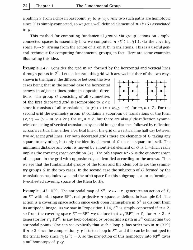
74 Chapter 1 The Fundamental Group
a path in Y from a chosen basepoint y0 to g(y0) . Any two such paths are homotopic
since Y is simply-connected, so we get a well-defined element of π1(Y/G) associated
to g .
This method for computing fundamental groups via group actions on simply-
connected spaces is essentially how we computed π1(S1) in §1.1, via the covering
space R→S1 arising from the action of Z on R by translations. This is a useful gen-
eral technique for computing fundamental groups, in fact. Here are some examples
illustrating this idea.
Example 1.42. Consider the grid in R2 formed by the horizontal and vertical lines
through points in Z2 . Let us decorate this grid with arrows in either of the two ways
shown in the figure, the difference between the two
cases being that in the second case the horizontal
arrows in adjacent lines point in opposite direc-
tions. The group G consisting of all symmetries
of the first decorated grid is isomorphic to Z×Z
since it consists of all translations (x,y)֏ (x +m,y + n) for m,n ∈ Z . For the
second grid the symmetry group G contains a subgroup of translations of the form
(x,y)֏ (x +m,y + 2n) for m,n ∈ Z , but there are also glide-reflection symme-
tries consisting of vertical translation by an odd integer distance followed by reflection
across a vertical line, either a vertical line of the grid or a vertical line halfway between
two adjacent grid lines. For both decorated grids there are elements of G taking any
square to any other, but only the identity element of G takes a square to itself. The
minimum distance any point is moved by a nontrivial element of G is 1, which easily
implies the covering space condition (∗) . The orbit space R2/G is the quotient space
of a square in the grid with opposite edges identified according to the arrows. Thus
we see that the fundamental groups of the torus and the Klein bottle are the symme-
try groups G in the two cases. In the second case the subgroup of G formed by the
translations has index two, and the orbit space for this subgroup is a torus forming a
two-sheeted covering space of the Klein bottle.
Example 1.43: RPn . The antipodal map of Sn , x֏ −x , generates an action of Z2
on Sn with orbit space RPn , real projective n space, as defined in Example 0.4. The
action is a covering space action since each open hemisphere in Sn is disjoint from
its antipodal image. As we saw in Proposition 1.14, Sn is simply-connected if n ≥ 2,
so from the covering space Sn→RPn we deduce that π1(RPn) ≈ Z2 for n ≥ 2. A
generator for π1(RPn) is any loop obtained by projecting a path in Sn connecting two
antipodal points. One can see explicitly that such a loop γ has order two in π1(RPn)
if n ≥ 2 since the composition γ γ lifts to a loop in Sn , and this can be homotoped to
the trivial loop since π1(Sn) = 0, so the projection of this homotopy into RPn gives
a nullhomotopy of γ γ .
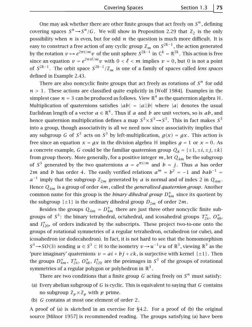
Covering Spaces Section 1.3 75
One may ask whether there are other finite groups that act freely on Sn , defining
covering spaces Sn→Sn/G . We will show in Proposition 2.29 that Z2 is the only
possibility when n is even, but for odd n the question is much more difficult. It is
easy to construct a free action of any cyclic group Zm on S2k−1 , the action generated
by the rotation v֏e2πi/mv of the unit sphere S2k−1 in Ck = R2k . This action is free
since an equation v = e2πiℓ/mv with 0 < ℓ < m implies v = 0, but 0 is not a point
of S2k−1 . The orbit space S2k−1/Zm is one of a family of spaces called lens spaces
defined in Example 2.43.
There are also noncyclic finite groups that act freely as rotations of Sn for odd
n > 1. These actions are classified quite explicitly in [Wolf 1984]. Examples in the
simplest case n = 3 can be produced as follows. View R4 as the quaternion algebra H .
Multiplication of quaternions satisfies |ab| = |a||b| where |a| denotes the usual
Euclidean length of a vector a ∈ R4 . Thus if a and b are unit vectors, so is ab , and
hence quaternion multiplication defines a map S3×S3→S3 . This in fact makes S3
into a group, though associativity is all we need now since associativity implies that
any subgroup G of S3 acts on S3 by left-multiplication, g(x) = gx . This action is
free since an equation x = gx in the division algebra H implies g = 1 or x = 0. As
a concrete example, G could be the familiar quaternion group Q8 = {±1,±i,±j,±k}
from group theory. More generally, for a positive integer m , let Q4m be the subgroup
of S3 generated by the two quaternions a = eπi/m and b = j . Thus a has order
2m and b has order 4. The easily verified relations am = b2= −1 and bab−1
=
a−1 imply that the subgroup Z2m generated by a is normal and of index 2 in Q4m .
Hence Q4m is a group of order 4m , called the generalized quaternion group. Another
common name for this group is the binary dihedral group D∗4m since its quotient by
the subgroup {±1} is the ordinary dihedral group D2m of order 2m .
Besides the groups Q4m = D∗4m there are just three other noncyclic finite sub-
groups of S3 : the binary tetrahedral, octahedral, and icosahedral groups T∗24 , O∗48,
and I∗120, of orders indicated by the subscripts. These project two-to-one onto the
groups of rotational symmetries of a regular tetrahedron, octahedron (or cube), and
icosahedron (or dodecahedron). In fact, it is not hard to see that the homomorphism
S3→SO(3) sending u ∈ S3⊂ H to the isometry v→u−1vu of R3 , viewing R3 as the
‘pure imaginary’ quaternions v = ai+ bj + ck , is surjective with kernel {±1} . Then
the groups D∗4m , T∗24 , O∗48 , I∗120 are the preimages in S3 of the groups of rotational
symmetries of a regular polygon or polyhedron in R3 .
There are two conditions that a finite group G acting freely on Sn must satisfy:
(a) Every abelian subgroup of G is cyclic. This is equivalent to saying that G contains
no subgroup Zp×Zp with p prime.
(b) G contains at most one element of order 2.
A proof of (a) is sketched in an exercise for §4.2. For a proof of (b) the original
source [Milnor 1957] is recommended reading. The groups satisfying (a) have been

76 Chapter 1 The Fundamental Group
completely classified; see [Brown 1982], section VI.9, for details. An example of a
group satisfying (a) but not (b) is the dihedral group D2m for odd m > 1.
There is also a much more difficult converse: A finite group satisfying (a) and (b)
acts freely on Sn for some n . References for this are [Madsen, Thomas, & Wall 1976]
and [Davis & Milgram 1985]. There is also almost complete information about which
n ’s are possible for a given group.
Example 1.44. In Example 1.35 we constructed a contractible 2 complex Xm,n =
Tm,n×R as the universal cover of a finite 2 complex Xm,n that was the union of
the mapping cylinders of the two maps S1→S1 , z֏ zm and z֏ zn . The group
of deck transformations of this covering space is therefore the fundamental group
π1(Xm,n) . From van Kampen’s theorem applied to the decomposition of Xm,n into
the two mapping cylinders we have the presentation⟨a,b |||| a
mb−n⟩
for this group
Gm,n = π1(Xm,n) . It is interesting to look at the action of Gm,n on Xm,n more closely.
We described a decomposition of Xm,n into rectangles, with Xm,n the quotient of
one rectangle. These rectangles in fact define a cell structure on Xm,n lifting a cell
structure on Xm,n with two vertices, three edges, and one 2 cell. The group Gm,n is
thus a group of symmetries of this cell structure on Xm,n . If we orient the three edges
of Xm,n and lift these orientations to the edges of Xm,n , then Gm,n is the group of all
symmetries of Xm,n preserving the orientations of edges. For example, the element a
acts as a ‘screw motion’ about an axis that is a vertical line {va}×R with va a vertex
of Tm,n , and b acts similarly for a vertex vb .
Since the action of Gm,n on Xm,n preserves the cell structure, it also preserves
the product structure Tm,n×R . This means that there are actions of Gm,n on Tm,nand R such that the action on the product Xm,n = Tm,n×R is the diagonal action
g(x,y) =(g(x), g(y)
)for g ∈ Gm,n . If we make the rectangles of unit height in the
R coordinate, then the element am = bn acts on R as unit translation, while a acts
by 1/m translation and b by 1/n translation. The translation actions of a and b on R
generate a group of translations of R that is infinite cyclic, generated by translation
by the reciprocal of the least common multiple of m and n .
The action of Gm,n on Tm,n has kernel consisting of the powers of the element
am = bn . This infinite cyclic subgroup is precisely the center of Gm,n , as we saw in
Example 1.24. There is an induced action of the quotient group Zm ∗ Zn on Tm,n ,
but this is not a free action since the elements a and b and all their conjugates fix
vertices of Tm,n . On the other hand, if we restrict the action of Gm,n on Tm,n to
the kernel K of the map Gm,n→Z given by the action of Gm,n on the R factor of
Xm,n , then we do obtain a free action of K on Tm,n . Since this action takes vertices
to vertices and edges to edges, it is a covering space action, so K is a free group, the
fundamental group of the graph Tm,n/K . An exercise at the end of the section is to
determine Tm,n/K explicitly and compute the number of generators of K .

Covering Spaces Section 1.3 77
Cayley Complexes
Covering spaces can be used to describe a very classical method for viewing
groups geometrically as graphs. Recall from Corollary 1.28 how we associated to each
group presentation G =⟨gα |||| rβ
⟩a 2 dimensional cell complex XG with π1(XG) ≈ G
by taking a wedge-sum of circles, one for each generator gα , and then attaching a
2 cell for each relator rβ . We can construct a cell complex XG with a covering space
action of G such that XG/G = XG in the following way. Let the vertices of XG be
the elements of G themselves. Then, at each vertex g ∈ G , insert an edge joining
g to ggα for each of the chosen generators gα . The resulting graph is known as
the Cayley graph of G with respect to the generators gα . This graph is connected
since every element of G is a product of gα ’s, so there is a path in the graph joining
each vertex to the identity vertex e . Each relation rβ determines a loop in the graph,
starting at any vertex g , and we attach a 2 cell for each such loop. The resulting cell
complex XG is the Cayley complex of G . The group G acts on XG by multiplication
on the left. Thus, an element g ∈ G sends a vertex g′ ∈ G to the vertex gg′ , and the
edge from g′ to g′gα is sent to the edge from gg′ to gg′gα . The action extends to
2 cells in the obvious way. This is clearly a covering space action, and the orbit space
is just XG .
In fact XG is the universal cover of XG since it is simply-connected. This can be
seen by considering the homomorphism ϕ :π1(XG)→G defined in the proof of Propo-
sition 1.39. For an edge eα in XG corresponding to a generator gα of G , it is clear
from the definition of ϕ that ϕ([eα]) = gα , so ϕ is an isomorphism. In particular
the kernel of ϕ , p∗(π1(XG)
), is zero, hence also π1(XG) since p∗ is injective.
Let us look at some examples of Cayley complexes.
Example 1.45. When G is the free group on
two generators a and b , XG is S1∨ S1 and
XG is the Cayley graph of Z∗ Z pictured at
the right. The action of a on this graph is a
rightward shift along the central horizontal
axis, while b acts by an upward shift along
the central vertical axis. The composition
ab of these two shifts then takes the vertex
e to the vertex ab . Similarly, the action of
any w ∈ Z∗ Z takes e to the vertex w .
Example 1.46. The group G = Z×Z with presentation⟨x,y |||| xyx
−1y−1 ⟩ has XGthe torus S1
×S1 , and XG is R2 with vertices the integer lattice Z2⊂ R
2 and edges
the horizontal and vertical segments between these lattice points. The action of G is
by translations (x,y)֏ (x +m,y +n) .
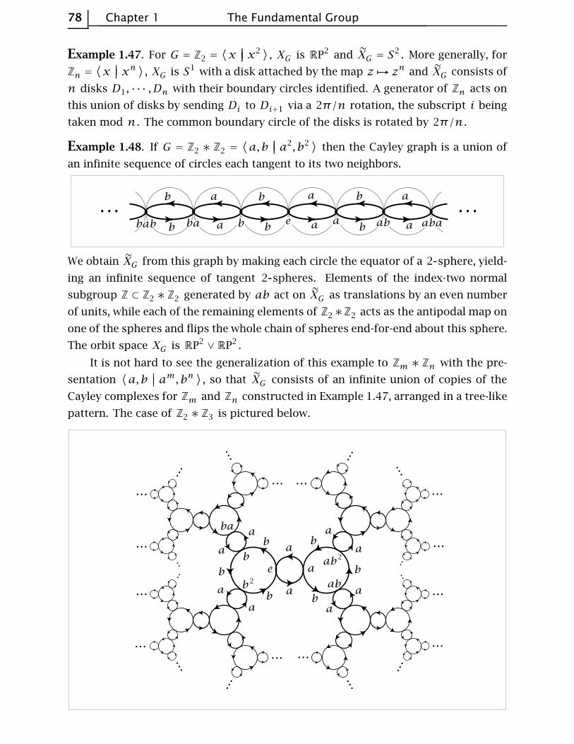
78 Chapter 1 The Fundamental Group
Example 1.47. For G = Z2 =⟨x |||| x
2 ⟩ , XG is RP2 and XG = S2 . More generally, for
Zn =⟨x |||| x
n ⟩ , XG is S1 with a disk attached by the map z֏zn and XG consists of
n disks D1, ··· ,Dn with their boundary circles identified. A generator of Zn acts on
this union of disks by sending Di to Di+1 via a 2π/n rotation, the subscript i being
taken mod n . The common boundary circle of the disks is rotated by 2π/n .
Example 1.48. If G = Z2 ∗ Z2 =⟨a,b |||| a
2, b2 ⟩ then the Cayley graph is a union of
an infinite sequence of circles each tangent to its two neighbors.
We obtain XG from this graph by making each circle the equator of a 2 sphere, yield-
ing an infinite sequence of tangent 2 spheres. Elements of the index-two normal
subgroup Z ⊂ Z2 ∗ Z2 generated by ab act on XG as translations by an even number
of units, while each of the remaining elements of Z2∗Z2 acts as the antipodal map on
one of the spheres and flips the whole chain of spheres end-for-end about this sphere.
The orbit space XG is RP2∨RP2 .
It is not hard to see the generalization of this example to Zm ∗ Zn with the pre-
sentation⟨a,b |||| a
m, bn⟩
, so that XG consists of an infinite union of copies of the
Cayley complexes for Zm and Zn constructed in Example 1.47, arranged in a tree-like
pattern. The case of Z2 ∗ Z3 is pictured below.
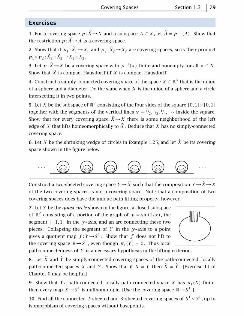
Covering Spaces Section 1.3 79
Exercises
1. For a covering space p : X→X and a subspace A ⊂ X , let A = p−1(A) . Show that
the restriction p : A→A is a covering space.
2. Show that if p1 : X1→X1 and p2 : X2→X2 are covering spaces, so is their product
p1×p2 : X1×X2→X1×X2 .
3. Let p : X→X be a covering space with p−1(x) finite and nonempty for all x ∈ X .
Show that X is compact Hausdorff iff X is compact Hausdorff.
4. Construct a simply-connected covering space of the space X ⊂ R3 that is the union
of a sphere and a diameter. Do the same when X is the union of a sphere and a circle
intersecting it in two points.
5. Let X be the subspace of R2 consisting of the four sides of the square [0,1]×[0,1]
together with the segments of the vertical lines x = 1/2,1/3,
1/4, ··· inside the square.
Show that for every covering space X→X there is some neighborhood of the left
edge of X that lifts homeomorphically to X . Deduce that X has no simply-connected
covering space.
6. Let X be the shrinking wedge of circles in Example 1.25, and let X be its covering
space shown in the figure below.
Construct a two-sheeted covering space Y→X such that the composition Y→X→Xof the two covering spaces is not a covering space. Note that a composition of two
covering spaces does have the unique path lifting property, however.
7. Let Y be the quasi-circle shown in the figure, a closed subspace
of R2 consisting of a portion of the graph of y = sin(1/x) , the
segment [−1,1] in the y axis, and an arc connecting these two
pieces. Collapsing the segment of Y in the y axis to a point
gives a quotient map f :Y→S1 . Show that f does not lift to
the covering space R→S1 , even though π1(Y ) = 0. Thus local
path-connectedness of Y is a necessary hypothesis in the lifting criterion.
8. Let X and Y be simply-connected covering spaces of the path-connected, locally
path-connected spaces X and Y . Show that if X ≃ Y then X ≃ Y . [Exercise 11 in
Chapter 0 may be helpful.]
9. Show that if a path-connected, locally path-connected space X has π1(X) finite,
then every map X→S1 is nullhomotopic. [Use the covering space R→S1 .]
10. Find all the connected 2 sheeted and 3 sheeted covering spaces of S1∨S1 , up to
isomorphism of covering spaces without basepoints.
80 Chapter 1 The Fundamental Group
11. Construct finite graphs X1 and X2 having a common finite-sheeted covering space
X1 = X2 , but such that there is no space having both X1 and X2 as covering spaces.
12. Let a and b be the generators of π1(S1∨ S1) corresponding to the two S1
summands. Draw a picture of the covering space of S1∨ S1 corresponding to the
normal subgroup generated by a2 , b2 , and (ab)4 , and prove that this covering space
is indeed the correct one.
13. Determine the covering space of S1∨ S1 corresponding to the subgroup of
π1(S1∨ S1) generated by the cubes of all elements. The covering space is 27 sheeted
and can be drawn on a torus so that the complementary regions are nine triangles
with edges labeled aaa , nine triangles with edges labeled bbb , and nine hexagons
with edges labeled ababab . [For the analogous problem with sixth powers instead
of cubes, the resulting covering space would have 228325 sheets! And for kth powers
with k sufficiently large, the covering space would have infinitely many sheets. The
underlying group theory question here, whether the quotient of Z ∗ Z obtained by
factoring out all kth powers is finite, is known as Burnside’s problem. It can also be
asked for a free group on n generators.]
14. Find all the connected covering spaces of RP2∨RP2 .
15. Let p : X→X be a simply-connected covering space of X and let A ⊂ X be a
path-connected, locally path-connected subspace, with A ⊂ X a path-component of
p−1(A) . Show that p : A→A is the covering space corresponding to the kernel of the
map π1(A)→π1(X) .
16. Given maps X→Y→Z such that both Y→Z and the composition X→Z are
covering spaces, show that X→Y is a covering space if Z is locally path-connected,
and show that this covering space is normal if X→Z is a normal covering space.
17. Given a group G and a normal subgroup N , show that there exists a normal
covering space X→X with π1(X) ≈ G , π1(X) ≈ N , and deck transformation group
G(X) ≈ G/N .
18. For a path-connected, locally path-connected, and semilocally simply-connected
space X , call a path-connected covering space X→X abelian if it is normal and has
abelian deck transformation group. Show that X has an abelian covering space that is
a covering space of every other abelian covering space of X , and that such a ‘universal’
abelian covering space is unique up to isomorphism. Describe this covering space
explicitly for X = S1∨ S1 and X = S1
∨ S1∨ S1 .
19. Use the preceding problem to show that a closed orientable surface Mg of genus
g has a connected normal covering space with deck transformation group isomorphic
to Zn (the product of n copies of Z ) iff n ≤ 2g . For n = 3 and g ≥ 3, describe such
a covering space explicitly as a subspace of R3 with translations of R3 as deck trans-
formations. Show that such a covering space in R3 exists iff there is an embedding

Covering Spaces Section 1.3 81
of Mg in the 3 torus T 3= S1
×S1×S1 such that the induced map π1(Mg)→π1(T
3)
is surjective.
20. Construct nonnormal covering spaces of the Klein bottle by a Klein bottle and by
a torus.
21. Let X be the space obtained from a torus S1×S1 by attaching a Mobius band via a
homeomorphism from the boundary circle of the Mobius band to the circle S1×{x0}
in the torus. Compute π1(X) , describe the universal cover of X , and describe the
action of π1(X) on the universal cover. Do the same for the space Y obtained by
attaching a Mobius band to RP2 via a homeomorphism from its boundary circle to
the circle in RP2 formed by the 1 skeleton of the usual CW structure on RP2 .
22. Given covering space actions of groups G1 on X1 and G2 on X2 , show that the ac-
tion of G1×G2 on X1×X2 defined by (g1, g2)(x1, x2) = (g1(x1), g2(x2)) is a covering
space action, and that (X1×X2)/(G1×G2) is homeomorphic to X1/G1×X2/G2 .
23. Show that if a group G acts freely and properly discontinuously on a Hausdorff
space X , then the action is a covering space action. (Here ‘properly discontinuously’
means that each x ∈ X has a neighborhood U such that {g ∈ G | U ∩ g(U) ≠∅} is
finite.) In particular, a free action of a finite group on a Hausdorff space is a covering
space action.
24. Given a covering space action of a group G on a path-connected, locally path-
connected space X , then each subgroup H ⊂ G determines a composition of covering
spaces X→X/H→X/G . Show:
(a) Every path-connected covering space between X and X/G is isomorphic to X/H
for some subgroup H ⊂ G .
(b) Two such covering spaces X/H1 and X/H2 of X/G are isomorphic iff H1 and H2
are conjugate subgroups of G .
(c) The covering space X/H→X/G is normal iff H is a normal subgroup of G , in
which case the group of deck transformations of this cover is G/H .
25. Let ϕ :R2→R2 be the linear transformation ϕ(x,y) = (2x,y/2) . This generates
an action of Z on X = R2− {0} . Show this action is a covering space action and
compute π1(X/Z) . Show the orbit space X/Z is non-Hausdorff, and describe how it is
a union of four subspaces homeomorphic to S1×R , coming from the complementary
components of the x axis and the y axis.
26. For a covering space p : X→X with X connected, locally path-connected, and
semilocally simply-connected, show:
(a) The components of X are in one-to-one correspondence with the orbits of the
action of π1(X,x0) on the fiber p−1(x0) .
(b) Under the Galois correspondence between connected covering spaces of X and
subgroups of π1(X,x0) , the subgroup corresponding to the component of X
82 Chapter 1 The Fundamental Group
containing a given lift x0 of x0 is the stabilizer of x0 , the subgroup consisting
of elements whose action on the fiber leaves x0 fixed.
27. For a universal cover p : X→X we have two actions of π1(X,x0) on the fiber
p−1(x0) , namely the action given by lifting loops at x0 and the action given by re-
stricting deck transformations to the fiber. Are these two actions the same when
X = S1∨ S1 or X = S1
×S1 ? Do the actions always agree when π1(X,x0) is abelian?
28. Show that for a covering space action of a group G on a simply-connected space
Y , π1(Y/G) is isomorphic to G . [If Y is locally path-connected, this is a special case
of part (b) of Proposition 1.40.]
29. Let Y be path-connected, locally path-connected, and simply-connected, and let
G1 and G2 be subgroups of Homeo(Y ) defining covering space actions on Y . Show
that the orbit spaces Y/G1 and Y/G2 are homeomorphic iff G1 and G2 are conjugate
subgroups of Homeo(Y ) .
30. Draw the Cayley graph of the group Z∗ Z2 =⟨a,b |||| b
2 ⟩ .
31. Show that the normal covering spaces of S1∨ S1 are precisely the graphs that
are Cayley graphs of groups with two generators. More generally, the normal cov-
ering spaces of the wedge sum of n circles are the Cayley graphs of groups with n
generators.
32. Consider covering spaces p : X→X with X and X connected CW complexes,
the cells of X projecting homeomorphically onto cells of X . Restricting p to the
1 skeleton then gives a covering space X1→X1 over the 1 skeleton of X . Show:
(a) Two such covering spaces X1→X and X2→X are isomorphic iff the restrictions
X11→X
1 and X12→X
1 are isomorphic.
(b) X→X is a normal covering space iff X1→X1 is normal.
(c) The groups of deck transformations of the coverings X→X and X1→X1 are
isomorphic, via the restriction map.
33. In Example 1.44 let d be the greatest common divisor of m and n , and let
m′= m/d and n′ = n/d . Show that the graph Tm,n/K consists of m′ vertices
labeled a , n′ vertices labeled b , together with d edges joining each a vertex to
each b vertex. Deduce that the subgroup K ⊂ Gm,n is free on dm′n′ −m′− n′ + 1
generators.

Graphs and Free Groups Section 1.A 83
Since all groups can be realized as fundamental groups of spaces, this opens the
way for using topology to study algebraic properties of groups. The topics in this
section and the next give some illustrations of this principle, mainly using covering
space theory.
We remind the reader that the Additional Topics which form the remainder of
this chapter are not to be regarded as an essential part of the basic core of the book.
Readers who are eager to move on to new topics should feel free to skip ahead.
By definition, a graph is a 1 dimensional CW complex, in other words, a space
X obtained from a discrete set X0 by attaching a collection of 1 cells eα . Thus X
is obtained from the disjoint union of X0 with closed intervals Iα by identifying the
two endpoints of each Iα with points of X0 . The points of X0 are the vertices and
the 1 cells the edges of X . Note that with this definition an edge does not include its
endpoints, so an edge is an open subset of X . The two endpoints of an edge can be
the same vertex, so the closure eα of an edge eα is homeomorphic either to I or S1 .
Since X has the quotient topology from the disjoint union X0∐α Iα , a subset of X
is open (or closed) iff it intersects the closure eα of each edge eα in an open (or closed)
set in eα . One says that X has the weak topology with respect to the subspaces eα .
In this topology a sequence of points in the interiors of distinct edges forms a closed
subset, hence never converges. This is true in particular if the edges containing the
sequence all have a common vertex and one tries to choose the sequence so that it
gets ‘closer and closer’ to the vertex. Thus if there is a vertex that is the endpoint
of infinitely many edges, then the weak topology cannot be a metric topology. An
exercise at the end of this section is to show the converse, that the weak topology is
a metric topology if each vertex is an endpoint of only finitely many edges.
A basis for the topology of X consists of the open intervals in the edges together
with the path-connected neighborhoods of the vertices. A neighborhood of the latter
sort about a vertex v is the union of connected open neighborhoods Uα of v in eαfor all eα containing v . In particular, we see that X is locally path-connected. Hence
a graph is connected iff it is path-connected.
If X has only finitely many vertices and edges, then X is compact, being the
continuous image of the compact space X0∐α Iα . The converse is also true, and more
generally, a compact subset C of a graph X can meet only finitely many vertices and
edges of X . To see this, let the subspace D ⊂ C consist of the vertices in C together
with one point in each edge that C meets. Then D is a closed subset of X since it
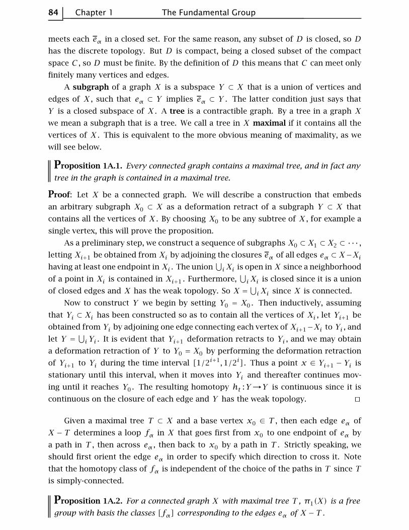
84 Chapter 1 The Fundamental Group
meets each eα in a closed set. For the same reason, any subset of D is closed, so D
has the discrete topology. But D is compact, being a closed subset of the compact
space C , so D must be finite. By the definition of D this means that C can meet only
finitely many vertices and edges.
A subgraph of a graph X is a subspace Y ⊂ X that is a union of vertices and
edges of X , such that eα ⊂ Y implies eα ⊂ Y . The latter condition just says that
Y is a closed subspace of X . A tree is a contractible graph. By a tree in a graph X
we mean a subgraph that is a tree. We call a tree in X maximal if it contains all the
vertices of X . This is equivalent to the more obvious meaning of maximality, as we
will see below.
Proposition 1A.1. Every connected graph contains a maximal tree, and in fact any
tree in the graph is contained in a maximal tree.
Proof: Let X be a connected graph. We will describe a construction that embeds
an arbitrary subgraph X0 ⊂ X as a deformation retract of a subgraph Y ⊂ X that
contains all the vertices of X . By choosing X0 to be any subtree of X , for example a
single vertex, this will prove the proposition.
As a preliminary step, we construct a sequence of subgraphs X0 ⊂ X1 ⊂ X2 ⊂ ··· ,
letting Xi+1 be obtained from Xi by adjoining the closures eα of all edges eα ⊂ X−Xihaving at least one endpoint in Xi . The union
⋃iXi is open in X since a neighborhood
of a point in Xi is contained in Xi+1 . Furthermore,⋃iXi is closed since it is a union
of closed edges and X has the weak topology. So X =⋃iXi since X is connected.
Now to construct Y we begin by setting Y0 = X0 . Then inductively, assuming
that Yi ⊂ Xi has been constructed so as to contain all the vertices of Xi , let Yi+1 be
obtained from Yi by adjoining one edge connecting each vertex of Xi+1−Xi to Yi , and
let Y =⋃i Yi . It is evident that Yi+1 deformation retracts to Yi , and we may obtain
a deformation retraction of Y to Y0 = X0 by performing the deformation retraction
of Yi+1 to Yi during the time interval [1/2i+1,1/2i] . Thus a point x ∈ Yi+1 − Yi is
stationary until this interval, when it moves into Yi and thereafter continues mov-
ing until it reaches Y0 . The resulting homotopy ht :Y→Y is continuous since it is
continuous on the closure of each edge and Y has the weak topology. ⊔⊓
Given a maximal tree T ⊂ X and a base vertex x0 ∈ T , then each edge eα of
X − T determines a loop fα in X that goes first from x0 to one endpoint of eα by
a path in T , then across eα , then back to x0 by a path in T . Strictly speaking, we
should first orient the edge eα in order to specify which direction to cross it. Note
that the homotopy class of fα is independent of the choice of the paths in T since T
is simply-connected.
Proposition 1A.2. For a connected graph X with maximal tree T , π1(X) is a free
group with basis the classes [fα] corresponding to the edges eα of X − T .
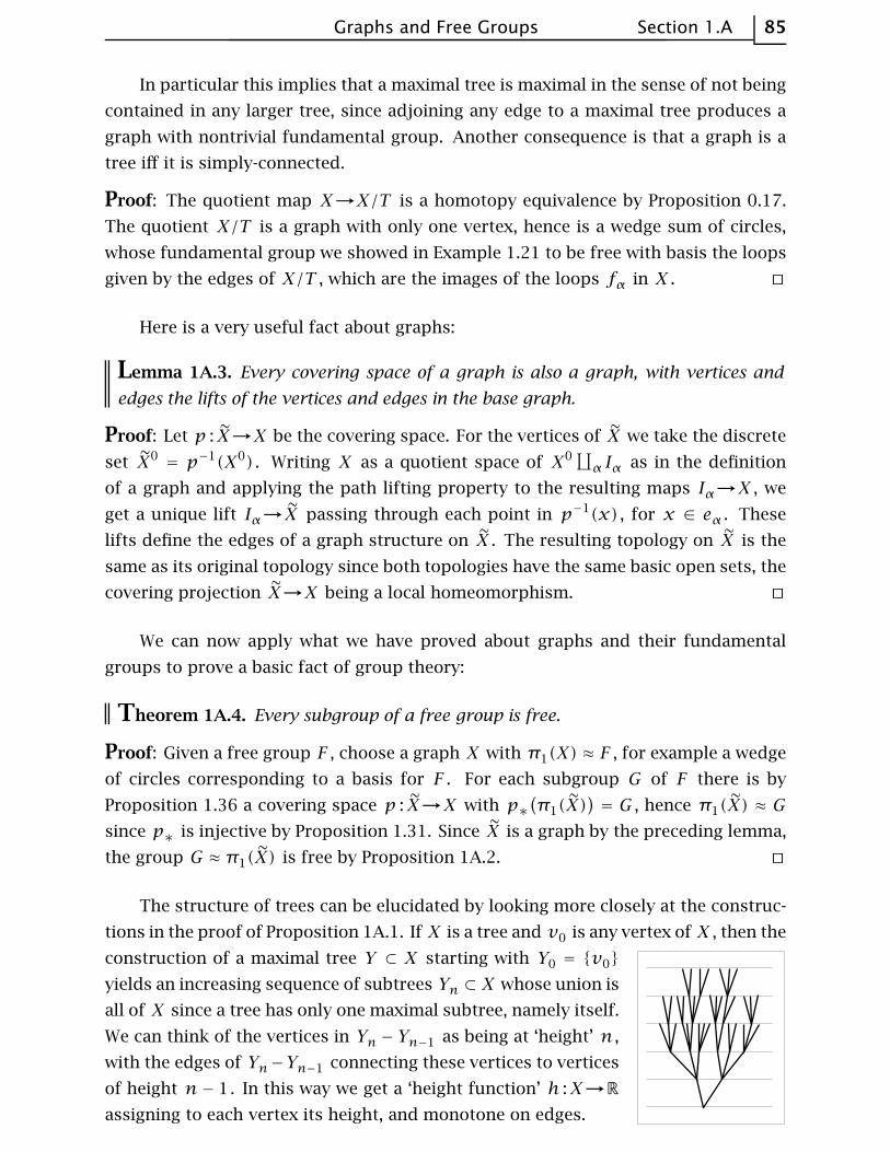
Graphs and Free Groups Section 1.A 85
In particular this implies that a maximal tree is maximal in the sense of not being
contained in any larger tree, since adjoining any edge to a maximal tree produces a
graph with nontrivial fundamental group. Another consequence is that a graph is a
tree iff it is simply-connected.
Proof: The quotient map X→X/T is a homotopy equivalence by Proposition 0.17.
The quotient X/T is a graph with only one vertex, hence is a wedge sum of circles,
whose fundamental group we showed in Example 1.21 to be free with basis the loops
given by the edges of X/T , which are the images of the loops fα in X . ⊔⊓
Here is a very useful fact about graphs:
Lemma 1A.3. Every covering space of a graph is also a graph, with vertices and
edges the lifts of the vertices and edges in the base graph.
Proof: Let p : X→X be the covering space. For the vertices of X we take the discrete
set X0= p−1(X0) . Writing X as a quotient space of X0
∐α Iα as in the definition
of a graph and applying the path lifting property to the resulting maps Iα→X , we
get a unique lift Iα→X passing through each point in p−1(x) , for x ∈ eα . These
lifts define the edges of a graph structure on X . The resulting topology on X is the
same as its original topology since both topologies have the same basic open sets, the
covering projection X→X being a local homeomorphism. ⊔⊓
We can now apply what we have proved about graphs and their fundamental
groups to prove a basic fact of group theory:
Theorem 1A.4. Every subgroup of a free group is free.
Proof: Given a free group F , choose a graph X with π1(X) ≈ F , for example a wedge
of circles corresponding to a basis for F . For each subgroup G of F there is by
Proposition 1.36 a covering space p : X→X with p∗(π1(X)
)= G , hence π1(X) ≈ G
since p∗ is injective by Proposition 1.31. Since X is a graph by the preceding lemma,
the group G ≈ π1(X) is free by Proposition 1A.2. ⊔⊓
The structure of trees can be elucidated by looking more closely at the construc-
tions in the proof of Proposition 1A.1. If X is a tree and v0 is any vertex of X , then the
construction of a maximal tree Y ⊂ X starting with Y0 = {v0}
yields an increasing sequence of subtrees Yn ⊂ X whose union is
all of X since a tree has only one maximal subtree, namely itself.
We can think of the vertices in Yn − Yn−1 as being at ‘height’ n ,
with the edges of Yn−Yn−1 connecting these vertices to vertices
of height n− 1. In this way we get a ‘height function’ h :X→R
assigning to each vertex its height, and monotone on edges.

86 Chapter 1 The Fundamental Group
For each vertex v of X there is exactly one edge leading downward from v , so
by following these downward edges we obtain a path from v to the base vertex v0 .
This is an example of an edgepath, which is a composition of finitely many paths each
consisting of a single edge traversed monotonically. For any edgepath joining v to v0
other than the downward edgepath, the height function would not be monotone and
hence would have local maxima, occurring when the edgepath backtracked, retracing
some edge it had just crossed. Thus in a tree there is a unique nonbacktracking
edgepath joining any two points. All the vertices and edges along this edgepath are
distinct.
A tree can contain no subgraph homeomorphic to a circle, since two vertices
in such a subgraph could be joined by more than one nonbacktracking edgepath.
Conversely, if a connected graph X contains no circle subgraph, then it must be a
tree. For if T is a maximal tree in X that is not equal to X , then the union of an edge
of X−T with the nonbacktracking edgepath in T joining the endpoints of this edge is
a circle subgraph of X . So if there are no circle subgraphs of X , we must have X = T ,
a tree.
For an arbitrary connected graph X and a pair of vertices v0 and v1 in X there is
a unique nonbacktracking edgepath in each homotopy class of paths from v0 to v1 .
This can be seen by lifting to the universal cover X , which is a tree since it is simply-
connected. Choosing a lift v0 of v0 , a homotopy class of paths from v0 to v1 lifts to
a homotopy class of paths starting at v0 and ending at a unique lift v1 of v1 . Then
the unique nonbacktracking edgepath in X from v0 to v1 projects to the desired
nonbacktracking edgepath in X .
Exercises
1. Let X be a graph in which each vertex is an endpoint of only finitely many edges.
Show that the weak topology on X is a metric topology.
2. Show that a connected graph retracts onto any connected subgraph.
3. For a finite graph X define the Euler characteristic χ(X) to be the number of
vertices minus the number of edges. Show that χ(X) = 1 if X is a tree, and that the
rank (number of elements in a basis) of π1(X) is 1− χ(X) if X is connected.
4. If X is a finite graph and Y is a subgraph homeomorphic to S1 and containing the
basepoint x0 , show that π1(X,x0) has a basis in which one element is represented
by the loop Y .
5. Construct a connected graph X and maps f , g :X→X such that fg = 11 but f
and g do not induce isomorphisms on π1 . [Note that f∗g∗ = 11 implies that f∗ is
surjective and g∗ is injective.]
6. Let F be the free group on two generators and let F ′ be its commutator subgroup.
Find a set of free generators for F ′ by considering the covering space of the graph
S1∨ S1 corresponding to F ′ .
K(G,1) Spaces and Graphs of Groups Section 1.B 87
7. If F is a finitely generated free group and N is a nontrivial normal subgroup of
infinite index, show, using covering spaces, that N is not finitely generated.
8. Show that a finitely generated group has only a finite number of subgroups of a
given finite index. [First do the case of free groups, using covering spaces of graphs.
The general case then follows since every group is a quotient group of a free group.]
9. Using covering spaces, show that an index n subgroup H of a group G has at most
n conjugate subgroups gHg−1 in G . Apply this to show that there exists a normal
subgroup K ⊂ G of finite index with K ⊂ H . [For the latter statement, consider
the intersection of all the conjugate subgroups gHg−1 . This is the maximal normal
subgroup of G contained in H .]
10. Let X be the wedge sum of n circles, with its natural graph structure, and let
X→X be a covering space with Y ⊂ X a finite connected subgraph. Show there is
a finite graph Z ⊃ Y having the same vertices as Y , such that the projection Y→Xextends to a covering space Z→X .
11. Apply the two preceding problems to show that if F is a finitely generated free
group and x ∈ F is not the identity element, then there is a normal subgroup H ⊂ F
of finite index such that x ∉ H . Hence x has nontrivial image in a finite quotient
group of F . In this situation one says F is residually finite.
12. Let F be a finitely generated free group, H ⊂ F a finitely generated subgroup, and
x ∈ F − H . Show there is a subgroup K of finite index in F such that K ⊃ H and
x ∉ K . [Apply Exercise 10.]
13. Let x be a nontrivial element of a finitely generated free group F . Show there is
a finite-index subgroup H ⊂ F in which x is one element of a basis. [Exercises 4 and
10 may be helpful.]
14. Show that the existence of maximal trees is equivalent to the Axiom of Choice.
In this section we introduce a class of spaces whose homotopy type depends only
on their fundamental group. These spaces arise many places in topology, especially
in its interactions with group theory.
A path-connected space whose fundamental group is isomorphic to a given group
G and which has a contractible universal covering space is called a K(G,1) space. The
‘1’ here refers to π1 . More general K(G,n) spaces are studied in §4.2. All these spaces
are called Eilenberg–MacLane spaces, though in the case n = 1 they were studied by
88 Chapter 1 The Fundamental Group
Hurewicz before Eilenberg and MacLane took up the general case. Here are some
examples:
Example 1B.1. S1 is a K(Z,1) . More generally, a connected graph is a K(G,1) with
G a free group, since by the results of §1.A its universal cover is a tree, hence con-
tractible.
Example 1B.2. Closed surfaces with infinite π1 , in other words, closed surfaces other
than S2 and RP2 , are K(G,1) ’s. This will be shown in Example 1B.14 below. It also
follows from the theorem in surface theory that the only simply-connected surfaces
without boundary are S2 and R2 , so the universal cover of a closed surface with
infinite fundamental group must be R2 since it is noncompact. Nonclosed surfaces
deformation retract onto graphs, so such surfaces are K(G,1) ’s with G free.
Example 1B.3. The infinite-dimensional projective space RP∞ is a K(Z2,1) since its
universal cover is S∞ , which is contractible. To show the latter fact, a homotopy from
the identity map of S∞ to a constant map can be constructed in two stages as follows.
First, define ft :R∞→R∞ by ft(x1, x2, ···) = (1 − t)(x1, x2, ···) + t(0, x1, x2, ···) .
This takes nonzero vectors to nonzero vectors for all t ∈ [0,1] , so ft/|ft| gives a ho-
motopy from the identity map of S∞ to the map (x1, x2, ···)֏(0, x1, x2, ···) . Then a
homotopy from this map to a constant map is given by gt/|gt| where gt(x1, x2, ···) =
(1− t)(0, x1, x2, ···)+ t(1,0,0, ···) .
Example 1B.4. Generalizing the preceding example, we can construct a K(Zm,1) as
an infinite-dimensional lens space S∞/Zm , where Zm acts on S∞ , regarded as the
unit sphere in C∞ , by scalar multiplication by mth roots of unity, a generator of this
action being the map (z1, z2, ···)֏ e2πi/m(z1, z2, ···) . It is not hard to check that
this is a covering space action.
Example 1B.5. A product K(G,1)×K(H,1) is a K(G×H,1) since its universal cover
is the product of the universal covers of K(G,1) and K(H,1) . By taking products of
circles and infinite-dimensional lens spaces we therefore get K(G,1) ’s for arbitrary
finitely generated abelian groups G . For example the n dimensional torus Tn , the
product of n circles, is a K(Zn,1) .
Example 1B.6. For a closed connected subspace K of S3 that is nonempty, the com-
plement S3−K is a K(G,1) . This is a theorem in 3 manifold theory, but in the special
case that K is a torus knot the result follows from our study of torus knot comple-
ments in Examples 1.24 and 1.35. Namely, we showed that for K the torus knot Km,nthere is a deformation retraction of S3
− K onto a certain 2 dimensional complex
Xm,n having contractible universal cover. The homotopy lifting property then implies
that the universal cover of S3− K is homotopy equivalent to the universal cover of
Xm,n , hence is also contractible.

K(G,1) Spaces and Graphs of Groups Section 1.B 89
Example 1B.7. It is not hard to construct a K(G,1) for an arbitrary group G , us-
ing the notion of a ∆ complex defined in §2.1. Let EG be the ∆ complex whose
n simplices are the ordered (n + 1) tuples [g0, ··· , gn] of elements of G . Such an
n simplex attaches to the (n− 1) simplices [g0, ··· , gi, ··· , gn] in the obvious way,
just as a standard simplex attaches to its faces. (The notation gi means that this
vertex is deleted.) The complex EG is contractible by the homotopy ht that slides
each point x ∈ [g0, ··· , gn] along the line segment in [e, g0, ··· , gn] from x to the
vertex [e] , where e is the identity element of G . This is well-defined in EG since
when we restrict to a face [g0, ··· , gi, ··· , gn] we have the linear deformation to [e]
in [e, g0, ··· , gi, ··· , gn] . Note that ht carries [e] around the loop [e, e] , so ht is not
actually a deformation retraction of EG onto [e] .
The group G acts on EG by left multiplication, an element g ∈ G taking the
simplex [g0, ··· , gn] linearly onto the simplex [gg0, ··· , ggn] . Only the identity e
takes any simplex to itself, so by an exercise at the end of this section, the action
of G on EG is a covering space action. Hence the quotient map EG→EG/G is the
universal cover of the orbit space BG = EG/G , and BG is a K(G,1) .
Since G acts on EG by freely permuting simplices, BG inherits a ∆ complex
structure from EG . The action of G on EG identifies all the vertices of EG , so BG
has just one vertex. To describe the ∆ complex structure on BG explicitly, note first
that every n simplex of EG can be written uniquely in the form
[g0, g0g1, g0g1g2, ··· , g0g1 ···gn] = g0[e, g1, g1g2, ··· , g1 ···gn]
The image of this simplex in BG may be denoted unambiguously by the symbol
[g1|g2| ··· |gn] . In this ‘bar’ notation the gi ’s and their ordered products can be
used to label edges, viewing an
edge label as the ratio between
the two labels on the vertices
at the endpoints of the edge,
as indicated in the figure. With
this notation, the boundary of
a simplex [g1| ··· |gn] of BG
consists of the simplices [g2| ··· |gn] , [g1| ··· |gn−1] , and [g1| ··· |gigi+1| ··· |gn]
for i = 1, ··· , n− 1.
This construction of a K(G,1) produces a rather large space, since BG is al-
ways infinite-dimensional, and if G is infinite, BG has an infinite number of cells in
each positive dimension. For example, BZ is much bigger than S1 , the most efficient
K(Z,1) . On the other hand, BG has the virtue of being functorial: A homomorphism
f :G→H induces a map Bf :BG→BH sending a simplex [g1| ··· |gn] to the simplex
[f (g1)| ··· |f(gn)] . A different construction of a K(G,1) is given in §4.2. Here one
starts with any 2 dimensional complex having fundamental group G , for example

90 Chapter 1 The Fundamental Group
the complex XG associated to a presentation of G , and then one attaches cells of di-
mension 3 and higher to make the universal cover contractible without affecting π1 .
In general, it is hard to get any control on the number of higher-dimensional cells
needed in this construction, so it too can be rather inefficient. Indeed, finding an
efficient K(G,1) for a given group G is often a difficult problem.
It is a curious and almost paradoxical fact that if G contains any elements of finite
order, then every K(G,1) CW complex must be infinite-dimensional. This is shown
in Proposition 2.45. In particular the infinite-dimensional lens space K(Zm,1) ’s in
Example 1B.4 cannot be replaced by any finite-dimensional complex.
In spite of the great latitude possible in the construction of K(G,1) ’s, there is a
very nice homotopical uniqueness property that accounts for much of the interest in
K(G,1) ’s:
Theorem 1B.8. The homotopy type of a CW complex K(G,1) is uniquely determined
by G .
Having a unique homotopy type of K(G,1) ’s associated to each group G means
that algebraic invariants of spaces that depend only on homotopy type, such as ho-
mology and cohomology groups, become invariants of groups. This has proved to be a
quite fruitful idea, and has been much studied both from the algebraic and topological
viewpoints. The discussion following Proposition 2.45 gives a few references.
The preceding theorem will follow easily from:
Proposition 1B.9. Let X be a connected CW complex and let Y be a K(G,1) . Then
every homomorphism π1(X,x0)→π1(Y ,y0) is induced by a map (X,x0)→(Y ,y0)
that is unique up to homotopy fixing x0 .
To deduce the theorem from this, let X and Y be CW complex K(G,1) ’s with iso-
morphic fundamental groups. The proposition gives maps f : (X,x0)→(Y ,y0) and
g : (Y ,y0)→(X,x0) inducing inverse isomorphisms π1(X,x0) ≈ π1(Y ,y0) . Then fg
and gf induce the identity on π1 and hence are homotopic to the identity maps.
Proof of 1B.9: Let us first consider the case that X has a single 0 cell, the base-
point x0 . Given a homomorphism ϕ :π1(X,x0)→π1(Y ,y0) , we begin the construc-
tion of a map f : (X,x0)→(Y ,y0) with f∗ = ϕ by setting f(x0) = y0 . Each 1 cell
e1α of X has closure a circle determining an element
[e1α] ∈ π1(X,x0) , and we let f on the closure of e1
α
be a map representing ϕ([e1α]) . If i :X1X denotes
the inclusion, then ϕi∗ = f∗ since π1(X1, x0) is gen-
erated by the elements [e1α] .
To extend f over a cell e2β with attaching map ψβ :S1→X1 , all we need is for the
composition fψβ to be nullhomotopic. Choosing a basepoint s0 ∈ S1 and a path in X1
from ψβ(s0) to x0 , ψβ determines an element [ψβ] ∈ π1(X1, x0) , and the existence

K(G,1) Spaces and Graphs of Groups Section 1.B 91
of a nullhomotopy of fψβ is equivalent to f∗([ψβ]) being zero in π1(Y ,y0) . We
have i∗([ψβ]) = 0 since the cell e2β provides a nullhomotopy of ψβ in X . Hence
f∗([ψβ]) = ϕi∗([ψβ]) = 0, and so f can be extended over e2β .
Extending f inductively over cells enγ with n > 2 is possible since the attaching
maps ψγ :Sn−1→Xn−1 have nullhomotopic compositions fψγ :Sn−1→Y . This is
because fψγ lifts to the universal cover of Y if n > 2, and this cover is contractible
by hypothesis, so the lift of fψγ is nullhomotopic, hence also fψγ itself.
Turning to the uniqueness statement, if two maps f0, f1 : (X,x0)→(Y ,y0) in-
duce the same homomorphism on π1 , then we see immediately that their restrictions
to X1 are homotopic, fixing x0 . To extend the resulting map X1×I ∪ X×∂I→Y
over the remaining cells en×(0,1) of X×I we can proceed just as in the preceding
paragraph since these cells have dimension n + 1 > 2. Thus we obtain a homotopy
ft : (X,x0)→(Y ,y0) , finishing the proof in the case that X has a single 0 cell.
The case that X has more than one 0 cell can be treated by a small elaboration
on this argument. Choose a maximal tree T ⊂ X . To construct a map f realizing a
given ϕ , begin by setting f(T) = y0 . Then each edge e1α in X − T determines an
element [e1α] ∈ π1(X,x0) , and we let f on the closure of e1
α be a map representing
ϕ([e1α]) . Extending f over higher-dimensional cells then proceeds just as before.
Constructing a homotopy ft joining two given maps f0 and f1 with f0∗ = f1∗ also
has an extra step. Let ht :X1→X1 be a homotopy starting with h0 = 11 and restricting
to a deformation retraction of T onto x0 . (It is easy to extend such a deformation
retraction to a homotopy defined on all of X1 .) We can construct a homotopy from
f0|X1 to f1|X
1 by first deforming f0|X1 and f1|X
1 to take T to y0 by composing with
ht , then applying the earlier argument to obtain a homotopy between the modified
f0|X1 and f1|X
1 . Having a homotopy f0|X1≃ f1|X
1 we extend this over all of X in
the same way as before. ⊔⊓
The first part of the preceding proof also works for the 2 dimensional complexes
XG associated to presentations of groups. Thus every homomorphism G→H is re-
alized as the induced homomorphism of some map XG→XH . However, there is no
uniqueness statement for this map, and it can easily happen that different presenta-
tions of a group G give XG ’s that are not homotopy equivalent.
Graphs of Groups
As an illustration of how K(G,1) spaces can be useful in group theory, we shall
describe a procedure for assembling a collection of K(G,1) ’s together into a K(G,1)
for a larger group G . Group-theoretically, this gives a method for assembling smaller
groups together to form a larger group, generalizing the notion of free products.
Let Γ be a graph that is connected and oriented, that is, its edges are viewed as
arrows, each edge having a specified direction. Suppose that at each vertex v of Γ we
92 Chapter 1 The Fundamental Group
place a group Gv and along each edge e of Γ we put a homomorphism ϕe from the
group at the tail of the edge to the group at the head of the edge. We call this data a
graph of groups. Now build a space BΓ by putting the space BGv from Example 1B.7
at each vertex v of Γ and then filling in a mapping cylinder of the map Bϕe along
each edge e of Γ , identifying the two ends of the mapping cylinder with the two BGv ’s
at the ends of e . The resulting space BΓ is then a CW complex since the maps Bϕetake n cells homeomorphically onto n cells. In fact, the cell structure on BΓ can be
canonically subdivided into a ∆ complex structure using the prism construction from
the proof of Theorem 2.10, but we will not need to do this here.
More generally, instead of BGv one could take any CW complex K(Gv ,1) at the
vertex v , and then along edges put mapping cylinders of maps realizing the homo-
morphisms ϕe . We leave it for the reader to check that the resulting space K Γ is
homotopy equivalent to the BΓ constructed above.
Example 1B.10. Suppose Γ consists of one central vertex with a number of edges
radiating out from it, and the group Gv at this central vertex is trivial, hence also all
the edge homomorphisms. Then van Kampen’s theorem implies that π1(K Γ ) is the
free product of the groups at all the outer vertices.
In view of this example, we shall call π1(K Γ ) for a general graph of groups Γ the
graph product of the vertex groups Gv with respect to the edge homomorphisms ϕe .
The name for π1(K Γ ) that is generally used in the literature is the rather awkward
phrase, ‘the fundamental group of the graph of groups’.
Here is the main result we shall prove about graphs of groups:
Theorem 1B.11. If all the edge homomorphisms ϕe are injective, then K Γ is a
K(G,1) and the inclusions K(Gv ,1)K Γ induce injective maps on π1 .
Before giving the proof, let us look at some interesting special cases:
Example 1B.12: Free Products with Amalgamation. Suppose the graph of groups is
A←C→B , with the two maps monomorphisms. One can regard this data as speci-
fying embeddings of C as subgroups of A and B . Applying van Kampen’s theorem
to the decomposition of K Γ into its two mapping cylinders, we see that π1(K Γ ) is
the quotient of A∗B obtained by identifying the subgroup C ⊂ A with the subgroup
C ⊂ B . The standard notation for this group is A ∗C B , the free product of A and
B amalgamated along the subgroup C . According to the theorem, A ∗C B contains
both A and B as subgroups.
For example, a free product with amalgamation Z ∗Z Z can be realized by map-
ping cylinders of the maps S1←S1→S1 that are m sheeted and n sheeted covering
spaces, respectively. We studied this case in Examples 1.24 and 1.35 where we showed
that the complex K Γ is a deformation retract of the complement of a torus knot in
S3 if m and n are relatively prime. It is a basic result in 3 manifold theory that the
K(G,1) Spaces and Graphs of Groups Section 1.B 93
complement of every smooth knot in S3 can be built up by iterated graph of groups
constructions with injective edge homomorphisms, starting with free groups, so the
theorem implies that these knot complements are K(G,1) ’s. Their universal covers
are all R3 , in fact.
Example 1B.13: HNN Extensions. Consider a graph of groups with ϕ
and ψ both monomorphisms. This is analogous to the previous case A←C→B ,
but with the two groups A and B coalesced to a single group. The group π1(K Γ ) ,which was denoted A ∗C B in the previous case, is now denoted A∗C . To see what
this group looks like, let us regard K Γ as being obtained from K(A,1) by attaching
K(C,1)×I along the two ends K(C,1)×∂I via maps realizing the monomorphisms
ϕ and ψ . Using a K(C,1) with a single 0 cell, we see that K Γ can be obtained from
K(A,1)∨S1 by attaching cells of dimension two and greater, so π1(K Γ ) is a quotient
of A∗Z , and it is not hard to figure out that the relations defining this quotient are of
the form tϕ(c)t−1= ψ(c) where t is a generator of the Z factor and c ranges over
C , or a set of generators for C . We leave the verification of this for the Exercises.
As a very special case, taking ϕ = ψ = 11 gives A∗A = A×Z since we can take
K Γ = K(A,1)×S1 in this case. More generally, taking ϕ = 11 with ψ an arbitrary
automorphism of A , we realize any semidirect product of A and Z as A∗A . For
example, the Klein bottle occurs this way, with ϕ realized by the identity map of S1
and ψ by a reflection. In these cases when ϕ = 11 we could realize the same group
π1(K Γ ) using a slightly simpler graph of groups, with a single vertex, labeled A , and
a single edge, labeled ψ .
Here is another special case. Suppose we take a torus, delete a small open disk,
then identify the resulting boundary circle with a longitudinal circle of the torus. This
produces a space X that happens to be homeomorphic to a subspace of the stan-
dard picture of a Klein bottle in R3 ; see Exercise 12 of §1.2. The fundamental group
π1(X) has the form (Z ∗ Z) ∗Z Z with the defining relation tb±1t−1= aba−1b−1
where a is a meridional loop and b is a longitudinal loop on the torus. The sign
of the exponent in the term b±1 is immaterial since the two ways of glueing the
boundary circle to the longitude produce homeomorphic spaces. The group π1(X) =⟨a,b, t |||| tbt
−1aba−1b−1 ⟩ abelianizes to Z×Z , but to show that π1(X) is not iso-
morphic to Z∗ Z takes some work. There is a surjection π1(X)→Z∗ Z obtained by
setting b = 1. This has nontrivial kernel since b is nontrivial in π1(X) by the pre-
ceding theorem. If π1(X) were isomorphic to Z∗ Z we would then have a surjective
homomorphism Z∗Z→Z∗Z that was not an isomorphism. However, it is a theorem
in group theory that a free group F is hopfian — every surjective homomorphism
F→F must be injective. Hence π1(X) is not free.
Example 1B.14: Closed Surfaces. A closed orientable surface M of genus two or
greater can be cut along a circle into two compact surfaces M1 and M2 such that the
94 Chapter 1 The Fundamental Group
closed surfaces obtained from M1 and M2 by filling in their boundary circle with a
disk have smaller genus than M . Each of M1 and M2 is the mapping cylinder of a
map from S1 to a finite graph. Namely, view Mi as obtained from a closed surface
by deleting an open disk in the interior of the 2 cell in the standard CW structure
described in Chapter 0, so that Mi becomes the mapping cylinder of the attaching
map of the 2 cell. This attaching map is not nullhomotopic, so it induces an injection
on π1 since free groups are torsionfree. Thus we have realized the original surface
M as K Γ for Γ a graph of groups of the form F1←------ Z -→F2 with F1 and F2 free and
the two maps injective. The theorem then says that M is a K(G,1) .
A similar argument works for closed nonorientable surfaces other than RP2 . For
example, the Klein bottle is obtained from two Mobius bands by identifying their
boundary circles, and a Mobius band is the mapping cylinder of the 2 sheeted covering
space S1→S1 .
Proof of 1B.11: We shall construct a covering space K→K Γ by gluing together copies
of the universal covering spaces of the various mapping cylinders in K Γ in such a way
that K will be contractible. Hence K will be the universal cover of K Γ , which will
therefore be a K(G,1) .
A preliminary observation: Given a universal covering space p : X→X and a con-
nected, locally path-connected subspace A ⊂ X such that the inclusion A X in-
duces an injection on π1 , then each component A of p−1(A) is a universal cover
of A . To see this, note that p : A→A is a covering space, so we have injective
maps π1(A)→π1(A)→π1(X) whose composition factors through π1(X) = 0, hence
π1(A) = 0. For example, if X is the torus S1×S1 and A is the circle S1
×{x0} , then
p−1(A) consists of infinitely many parallel lines in R2 , each a universal cover of A .
For a map f :A→B between connected CW complexes, let p : Mf→Mf be the
universal cover of the mapping cylinder Mf . Then Mf is itself the mapping cylinder
of a map f :p−1(A)→p−1(B) since the line segments in the mapping cylinder struc-
ture on Mf lift to line segments in Mf defining a mapping cylinder structure. Since
Mf is a mapping cylinder, it deformation retracts onto p−1(B) , so p−1(B) is also
simply-connected, hence is the universal cover of B . If f induces an injection on π1 ,
then the remarks in the preceding paragraph apply, and the components of p−1(A)
are universal covers of A . If we assume further that A and B are K(G,1) ’s, then Mfand the components of p−1(A) are contractible, and we claim that Mf deformation
retracts onto each component A of p−1(A) . Namely, the inclusion AMf is a homo-
topy equivalence since both spaces are contractible, and then Corollary 0.20 implies
that Mf deformation retracts onto A since the pair (Mf , A) satisfies the homotopy
extension property, as shown in Example 0.15.
Now we can describe the construction of the covering space K of K Γ . It will be
the union of an increasing sequence of spaces K1 ⊂ K2 ⊂ ··· . For the first stage,
let K1 be the universal cover of one of the mapping cylinders Mf of K Γ . By the

K(G,1) Spaces and Graphs of Groups Section 1.B 95
preceding remarks, this contains various disjoint copies of universal covers of the
two K(Gv ,1) ’s at the ends of Mf . We build K2 from K1 by attaching to each of these
universal covers of K(Gv ,1) ’s a copy of the universal cover of each mapping cylinder
Mg of K Γ meeting Mf at the end of Mf in question. Now repeat the process to
construct K3 by attaching universal covers of mapping cylinders at all the universal
covers of K(Gv ,1) ’s created in the previous step. In the same way, we construct Kn+1
from Kn for all n , and then we set K =⋃n Kn .
Note that Kn+1 deformation retracts onto Kn since it is formed by attaching
pieces to Kn that deformation retract onto the subspaces along which they attach,
by our earlier remarks. It follows that K is contractible since we can deformation
retract Kn+1 onto Kn during the time interval [1/2n+1,1/2n] , and then finish with a
contraction of K1 to a point during the time interval [1/2,1].
The natural projection K→K Γ is clearly a covering space, so this finishes the
proof that K Γ is a K(G,1) .
The remaining statement that each inclusion K(Gv ,1)K Γ induces an injection
on π1 can easily be deduced from the preceding constructions. For suppose a loop
γ :S1→K(Gv ,1) is nullhomotopic in K Γ . By the lifting criterion for covering spaces,
there is a lift γ :S1→K . This has image contained in one of the copies of the universal
cover of K(Gv ,1) , so γ is nullhomotopic in this universal cover, and hence γ is
nullhomotopic in K(Gv ,1) . ⊔⊓
The various mapping cylinders that make up the universal cover of K Γ are ar-
ranged in a treelike pattern. The tree in question, call it T Γ , has one vertex for each
copy of a universal cover of a K(Gv ,1) in K , and two vertices are joined by an edge
whenever the two universal covers of K(Gv ,1) ’s corresponding to these vertices are
connected by a line segment lifting a line segment in the mapping cylinder structure of
a mapping cylinder of K Γ . The inductive construction of K is reflected in an inductive
construction of T Γ as a union of an increasing sequence of subtrees T1 ⊂ T2 ⊂ ··· .
Corresponding to K1 is a subtree T1 ⊂ T Γ consisting of a central vertex with a number
of edges radiating out from it, an ‘asterisk’ with possibly an infinite number of edges.
When we enlarge K1 to K2 , T1 is correspondingly enlarged to a tree T2 by attaching
a similar asterisk at the end of each outer vertex of T1 , and each subsequent enlarge-
ment is handled in the same way. The action of π1(K Γ ) on K as deck transformations
induces an action on T Γ , permuting its vertices and edges, and the orbit space of T Γunder this action is just the original graph Γ . The action on T Γ will not generally
be a free action since the elements of a subgroup Gv ⊂ π1(K Γ ) fix the vertex of T Γcorresponding to one of the universal covers of K(Gv ,1) .
There is in fact an exact correspondence between graphs of groups and groups
acting on trees. See [Scott & Wall 1979] for an exposition of this rather nice theory.
From the viewpoint of groups acting on trees, the definition of a graph of groups is
96 Chapter 1 The Fundamental Group
usually taken to be slightly more restrictive than the one we have given here, namely,
one considers only oriented graphs obtained from an unoriented graph by subdividing
each edge by adding a vertex at its midpoint, then orienting the two resulting edges
outward, away from the new vertex.
Exercises
1. Suppose a group G acts simplicially on a ∆ complex X , where ‘simplicially’ means
that each element of G takes each simplex of X onto another simplex by a linear
homeomorphism. If the action is free, show it is a covering space action.
2. Let X be a connected CW complex and G a group such that every homomorphism
π1(X)→G is trivial. Show that every map X→K(G,1) is nullhomotopic.
3. Show that every graph product of trivial groups is free.
4. Use van Kampen’s theorem to compute A∗C as a quotient of A ∗ Z , as stated in
the text.
5. Consider the graph of groups Γ having one vertex, Z , and one edge, the map Z→Z
that is multiplication by 2, realized by the 2 sheeted covering space S1→S1 . Show
that π1(K Γ ) has presentation⟨a,b |||| bab
−1a−2 ⟩ and describe the universal cover
of K Γ explicitly as a product T×R with T a tree. [The group π1(K Γ ) is the first in
a family of groups called Baumslag-Solitar groups, having presentations of the form⟨a,b |||| ba
mb−1a−n⟩
. These are HNN extensions Z∗Z .]
6. Show that for a graph of groups all of whose edge homomorphisms are injective
maps Z→Z , we can choose K Γ to have universal cover a product T×R with T a
tree. Work out in detail the case that the graph of groups is the infinite sequence
Z2-----→ Z
3-----→ Z
4-----→ Z -→ ··· where the map Z
n-----→ Z is multiplication by n . Show
that π1(K Γ ) is isomorphic to Q in this case. How would one modify this example
to get π1(K Γ ) isomorphic to the subgroup of Q consisting of rational numbers with
denominator a power of 2?
7. Show that every graph product of groups can be realized by a graph whose vertices
are partitioned into two subsets, with every oriented edge going from a vertex in the
first subset to a vertex in the second subset.
8. Show that a finite graph product of finitely generated groups is finitely generated,
and similarly for finitely presented groups.
9. If Γ is a finite graph of finite groups with injective edge homomorphisms, show that
the graph product of the groups has a free subgroup of finite index by constructing
a suitable finite-sheeted covering space of K Γ from universal covers of the mapping
cylinders in K Γ . [The converse is also true: A finitely generated group having a free
subgroup of finite index is isomorphic to such a graph product. For a proof of this
see [Scott & Wall 1979], Theorem 7.3.]