the huges array co-processor and its application to robotics
TRANSCRIPT
University of Pennsylvania University of Pennsylvania
ScholarlyCommons ScholarlyCommons
Technical Reports (CIS) Department of Computer & Information Science
February 1991
The Huges Array Co-Processor and Its Application to Robotics The Huges Array Co-Processor and Its Application to Robotics
Craig Sayers University of Pennsylvania
Follow this and additional works at: https://repository.upenn.edu/cis_reports
Recommended Citation Recommended Citation Craig Sayers, "The Huges Array Co-Processor and Its Application to Robotics", . February 1991.
University of Pennsylvania Department of Computer and Information Science Technical Report No. MS-CIS-91-17.
This paper is posted at ScholarlyCommons. https://repository.upenn.edu/cis_reports/487 For more information, please contact [email protected].
The Huges Array Co-Processor and Its Application to Robotics The Huges Array Co-Processor and Its Application to Robotics
Abstract Abstract This report describes the results of twelve months research involving the Hughes array co-processor. This work began with the testing and debugging of the existing system, continued with the development of software to interface the co-processor to a host machine and concluded with the implementation of a trajectory planning algorithm for redundant manipulators.
A loader program has been developed which allows simple programs to be executed. A library of C-callable routines has also been created and this enables the fabrication of more complex systems which require a high level of interaction between the host and co-processor.
Routines to perform square root, sine and cosine functions have been designed and these have been used successfully in the development of a trajectory planning algorithm. This algorithm uses the co-processor to compute in parallel a large number of forward kinematics solutions and by doing so is able to convert a cartesian space trajectory into a joint space path for a redundant manipulator.
The performance of the processor has been analyzed and a number of recommendations have been made concerning future implementations.
Comments Comments University of Pennsylvania Department of Computer and Information Science Technical Report No. MS-CIS-91-17.
This technical report is available at ScholarlyCommons: https://repository.upenn.edu/cis_reports/487
The Huges Array Co-Processor and Its Application To Robotics
MS-CIS-91-17 GRASP LAB 255
Craig Sayers
Department of Computer and Information Science School of Engineering and Applied Science
University of Pennsylvania Philadelphia, PA 19104-6389
February 1991
The Hughes Array CoPmmssor and its Application to Robotics.
Craig Sayers
O 1991, The University of Pennsylvania, Philadelphia PA 19104, U.S.A.
This work was supported by the National Science Foundation under Grant Number
MIP87-14689. Any opinions, findings, conclusions or recommendations expressed in this
report are those of the author and do not necessarily reflect the views of the National Science
Foundation.
This report describes the results of twelve months research involving the Hughes array co-processor. This work began with the testing and
debugging of the existing system, continued with the development of
software to interface the co-processor to a host machine and concluded with
the implementation of a trajectory planning algorithm for redundant
manipulators.
A loader program has been developed which allows simple programs t o be
executed. A library of C-callable routines has also been created and this
enables the fabrication of more complex systems which require a high level
of interaction between the host and co-processor.
Routines to perform square root, sine and cosine functions have been
designed and these have been used successfully in the development of a
trajectory planning algorithm. This algorithm uses the co-processor t o compute in parallel a large number of forward kinematics solutions and by
doing so is able to convert a cartesian space trajectory into a joint space path
for a redundant manipulator.
The performance of the processor has been analysed and a number of
recommendations have been made concerning future implementations.
Acknowledgements
The author wishes to thank Janez Funda for his assistance with regard t o the use of the simulator and Charles Martin and K.Wojtek Przytula for
their invaluable help in correcting hardware related errors.
Contents
.............................................................................. 1 . Introduction 6
2 . Hardware .................................................................................. 8 ........................................... 2.1 An Overview of the Processor 8
2.2 The Connection t o a Host Machine ....................................... 9 2.3 The Processing Elements ................................................... 9
3 . Description of the Development Environment ................................ 14 ......................................................... 3.1 The Loader Program 14
3.2 The Library of C-callable routines ....................................... l 5 ....................................................... 3.3 An Example Program 19
.................................. 4 . Writing Software for the Hughes Prw:essor 22 ........................................................................ 4.1 Overview -22
.......................................................... 4.2 Optimising the code 23
......................................... 5 . Description of the Square Root Routine 25 ........................................................................ 5.1 Overview -25
5.2 Algorithmic Description .................................................... 26 .............................................................. 5.3 Range Reduction 27
5.4 ChoosinganInitialGuess ................................................. 27 5.5 The Complete Algorithm ................................................... 33
..................................................... 5.6 Results and Discussion 34
................................... 6 . Description of the Sine and Cosine Routine 36 ........................................................................ 6.1 Overview -36
.................................................... 6.2 Algorithmic Description 36 6.3 Results and Discussion ..................................................... 38
7 . Application to ~ ' e c t o r y Planning for Redundant Manipulators ................................................................... 40
7.1 Overview ........................................................................ -40 .................................. 7.2 Implementation on the Co-processor 42
.............................................. 7.3 Implementation on the Host 44 ..................................................... 7.4 Results and Discussion 44
8 . Discussion and Suggested Design Modifications ........................... 54 ........................................................................ 8.1 Hardware 54
8.2 Software ......................................................................... -56
.............................................................................. 9 . Conclusions 58
.............................................. Appendix A . The Testing Process -59
........................ Appendix B . Software for the Square Root Routine 61
Appendix C . SoRware for the SinICos Routine .............................. ............................. Appendix D . Software for Trajectory Planning 72
The Hughes array co-processor is the result of a joint effort between Hughes Research Laboratories and the University of Pennsylvania. The hardware
was developed a t Hughes by Ted Carmely, Lap Wai Chow, Charles Martin, J.Greg Nash, K. Wojtek Pryztula and Dale Simpa. The software development system was created a t the University of Pennsylvania GRASP Lab by Miriam Hartholtz (assembler) and Janez Funda (simulator).
This report describes the results of twelve months of research involving the Hughes array co-processor. In its initial stages this work involved the testing and debugging of the existing system ( see Appendix A ). Subsequent research was aimed at the development of software t o allow for a high level of interaction between the co-processor and the host machine. A number of routines were developed to run on the co-processor and this work culminated in the implementation of a trajectory planning algorithm for redundant manipulators.
Section two of the report describes the machine at the hardware level and includes a detailed analysis of the major functional units. This will prove important in the investigation of errors produced by the software described later in the report.
The third section describes the addition of both a loader and a library of C-
callable routines to the software development environment. The loader allows small stand-alone programs to be executed on the processor while the C-callable routines provide the means by which more complex programs may be constructed. By way of example a simple addition program is presented.
The fourth section of this report discusses some of the less obvious factors involved in developing software for the co-processor. In particular the selection of appropriate algorithms and the programming methodology involved in turning such algorithms into efficient working programs are described.
Section five describes the implementation of a square-root routine on the
processor. Such a routine is required for a number of applications yet its implementation is non-trivial due to the unique hardware constraints inherent in the array co-processor.
The sixth section focuses on the development of a single routine to calculate sine and cosine values. This will form the basis for the forward kinematics solution used in the trajectory planning application.
Section seven describes the development of trajectory planning scheme for redundant manipulators. This application makes good use of the parallelism inherent in the array and also demonstrates the practicality of
splitting the work-load between the array co-processor and the host machine.
Section eight provides a discussion of possible improvements t o both the hardware and software of the current system. It is intended that this
discussion should provide some direction for future work.
2. Hardware
The hardware component of the Hughes co-processor has already been described in some detail [I] and this section of the report is intended t o complement this existing documentation. A brief description of the hardware will be presented followed by an in depth look at the current performance of the functional units within each processing element. Such an analysis is fundamental t o the understanding of errors in the mathematical routines described later in the report.
2.1 An Ovemiew of the Processor
The Hughes co-processor is composed of 256 processing elements configured in a square 16x16 array. Systolic architectures of the type originally proposed by Kung[2] are typically made up of a number of simple processing elements - each of which is dedicated to a simple task. Data is manipulated by feeding it into the array at the array boundaries. The data is then continuously processed as it moves through the array with the results appearing at the output of boundary processing elements on the far side of the array. The Hughes processor differs a little from this definition in that each processing element is a programmable arithmetic logic unit.
In effect this makes the processor into what Kung[3] terms a
"programmable systolic array". While this will clearly not be as efficient as
a dedicated system it does have the significant advantage of allowing the same hardware to be used for a number of applications.
1 Przytula, K.W., Systolic Cellular System, Hughes Research Laboratories, March 1988.
2 Kung, H.T., "Why Systolic Architectures", IEEE Computer, Jan, 1982, pp37-46.
3 Kung, H.T., "On the Implementation and use of Systolic Array Processors", Proc. IEEE Int. Conference on Computer Design, Port Chester, N.Y., 1983, pp370-373.
2.2 The Connection to a Host Machine
The host machine ( a Sun workstation ) communicates with the co- processor through a VME connection by means of a memory-mapped interface. The processor data and program memories appear as the Sun's own memory and may be read from, or written to, directly ( see Figure 2.2).
Figure 2.2 An overview of the array mpmcessor and its connection to the host machine ( the fVo queues are not shown in this simplified view 1.
The host controls the co-processor by reading or writing specific memory addresses. These accesses are detected by the processor and interpreted as command signals. As a result the controlling program will often contain several readdwrites to the same memory location and care must be taken to ensure that an over-zealous optimising compiler does not mistakenly consider these commands to be superfluous.
I
Program Memory
w
Interface to Host Machine
2.3 The Processing Elements
b
Each processing element is composed of four input/output ports, 24 static registers and six functional units. These components are connected by two buses ( see Figure 2.3.1 ).
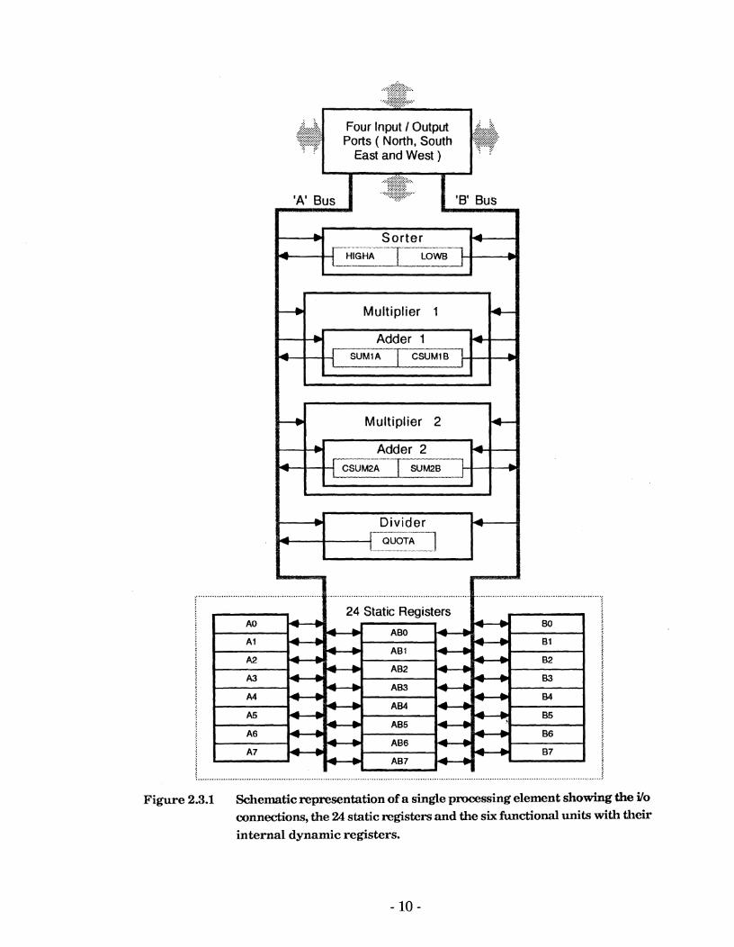
Figure 2.3.1 Schematic representation of a single pmss ing element showing the ilo connections, the 24 static registers and the six functional units with their internal dynamic registers.
The inputloutput ports facilitate connection to each of the four nearest- neighbour processing elements in the square array and are logically termed the West, East, North and South ports. The West port of the Western-most processing elements are connected to the East port of the Eastern-most processing elements. This is logically equivalent to folding the array into a cylinder about a North-South axis. The North port of the Northern-most processing elements receives input from the data memory, while the South port of the Southern-most elements may be used to write t o data memory. In most cases input data will move from the data memory into the processing array via the Northern-most elements. It will then pass
through the array in a Southerly direction while being processed by the functional units within each element. The final results will eventually appear a t the Southern-most processing elements from where they may be written into the data memory. More complex arrangements are also
possible. For example it is possible to write results to data memory from the Southern edge of the array and then read those same results back into the Northern edge. This is logically equivalent to folding the array into a cylinder about the east-west axis.
The 24 static registers are split into three groups of eight. The first being accessible from either bus, the second only from bus A and the third only
from bus B. In practice the limitation than two thirds of the registers can
only be accessed from one bus is not a major inconvenience but it does mean than some care must be taken when assigning logical variables to physical registers.
The six functional units are a sorter, divider, two adders and two multipliers. The two inputs to each functional unit are provided via the two buses and the output(s) are stored in dynamic output registers within each functional unit. These dynamic registers do not retain their values indefinitely and care must be taken to ensure that results are read before they decay away. The inputs may come either from the static registers or from the dynamic output registers in each functional unit. This means that intermediate values need not be stored in static registers and may
instead be passed directly from the output of one functional unit to the input
of another. For example its possible to use multiplier one to calculate the
product of the previous result from multiplier one and the previous sum from the second adder.
The sorter takes one input from each bus, sorts them and stores the result in two dynamic registers. No problems were found with the sorter during testing.
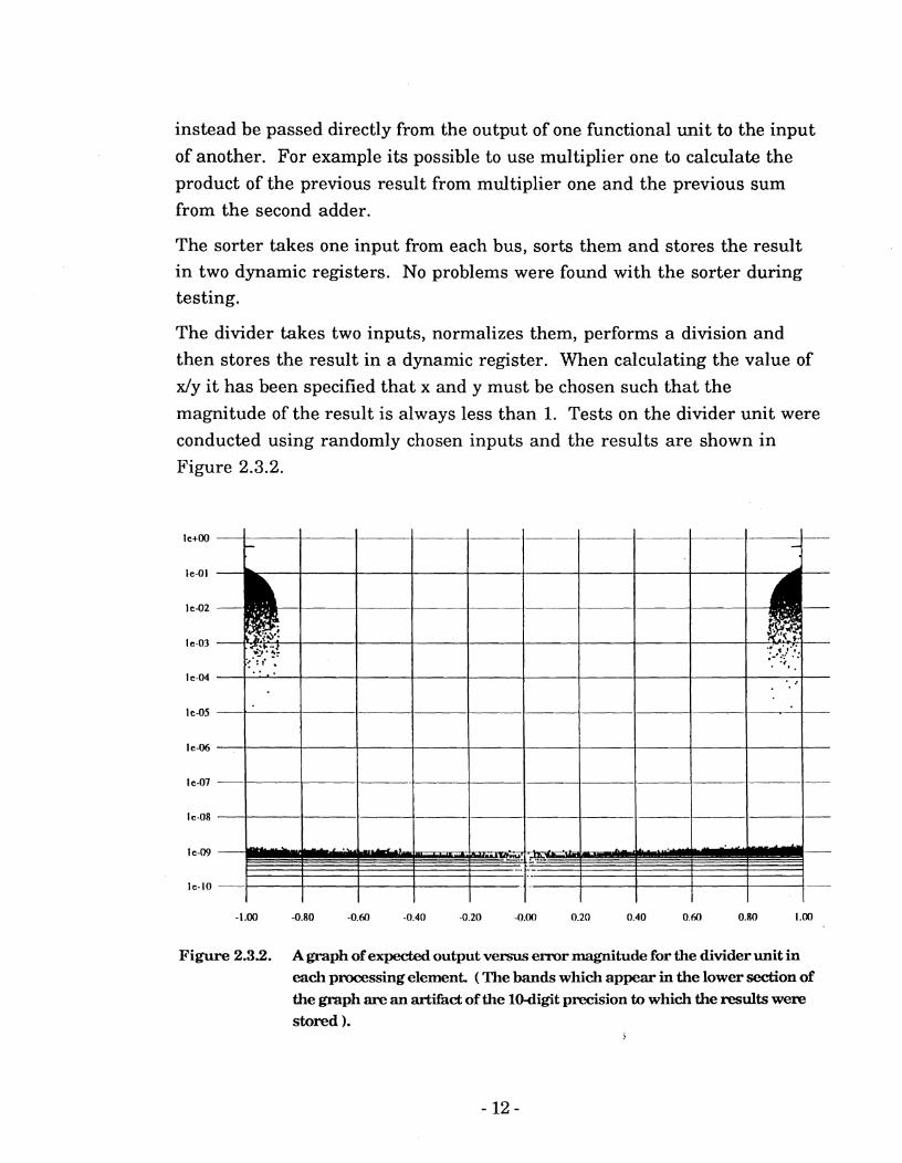
The divider takes two inputs, normalizes them, performs a division and then stores the result in a dynamic register. When calculating the value of x/y i t has been specified that x and y must be chosen such that the
magnitude of the result is always less than 1. Tests on the divider unit were conducted using randomly chosen inputs and the results are shown in
Figure 2.3.2.
Figure 2.3.2. A graph of expected output versus e m r magnitude for the divider unit in each processing element. ( The bands which appear in the lower section of the graph are an artifact of the lo-digit precision to which the results were stored 1.
Examination of the above graph shows that the result is unreliable whenever the magnitude of the expected result is greater than 0.875. Provided this limit is not exceeded then reasonably good results are obtained. However, even in these cases the error is still greater than might be expected.
Each of the two adders takes two inputs ( one via each bus ) and stores their sum and its complement in two dynamic registers which are each accessible via one of the buses. Tests on the adders showed no errors in the output.
Each of the two multipliers takes two inputs ( again one from each bus) and produces two partial products. These are then summed in the adders t o produce the final product and its complement which are stored in two dynamic registers. The two multipliers can be used in parallel to multiply two different pairs of numbers and this configuration was found t o be particularly useful ( see the sine and cosine routines for example).
Tests on the output from the multipliers failed t o reveal any substantial errors however it was found that the least significant two bits of the resulting word were often incorrect.
3. Description of the Development Environment.
The development environment previously consisted of an assembler and a
simulator. Since both of these have already been well documented [4,51 this section of the report will concentrate on describing the two new additions to the system: a loader and a library of C-callable routines. An example program which demonstrates the transfer of data to and from the co- processor is also presented.
3.1 The Loader Program
The loader program simplifies the task of writing and testing simple
programs for the Hughes system. It can load the processor data memory with input data, load the program memory and fifo queues with instructions from an assembler-generated executable file, run the program and then create an output file by reading values from the processor data memory.
This process is set in motion by typing the command:
load [-h] filename
Where filename is the name of a control file. This file contains all the information which the loader program requires and it allows the process to be carried out independently of further operator action.
The format for the control file is:
executable-data-filename
input - data-filename
output - data-filename
first-row-of-output-data
last-row-of-output-data
4 Hartholz, M.A., The SystoliclCellular System Assembler: User's Guide, Master's Thesis, The University of Pennsylvania, August, 1988.
5 Funda, J., Symbolic SimulatorIDebugger for the SystoliclCellular Array Processor, The University of Pennsylvania, January, 1991, Technical Report #
MS-CIS-9 1-07
Where input-data-filename is the name of a file containing the data values with which the array is to be initialized. The format for this file is identical to the data file used by the simulator with the addition that data values may be in either floating-point or hexadecimal format. When called with the -h option the input file is assumed to be in hexadecimal format and the output file is created in hexadecimal format. Alternatively if the -h switch is not
specified then both files are in floating-point format.
The executable-data-filename is the name of an output file created by the assembler.
Once the program has been executed the loader reads values from data memory in the range first-row-of-output-data through last-row-of-output-data and writes them to the file output-data-filename using the format specified by the presence or absence of the -h switch.
The loader is intended to facilitate the testing of simple stand-alone
programs. However, to access the full power of the array co-processor it is necessary to have a finer level of control over the hardware and it is particularly desirable to have a greater level of interaction between the host and co-processor. It was to provide this additional power that a library of C- callable routines was created.
3.2 The Library of C-callable routines
The library of C-callable routines allows a programmer to have a high level
of control over the co-processor without necessarily needing to have a
detailed understanding of the underlying hardware. A description of these routines will be followed by an example of their use.
There is no elegant way to recover from most processor-related errors. As a result the following routines handle errors by printing an error text to stderr and then exiting with code 1.
This routine opens the VME device driver, allocates memory space for the co-processor and maps that space into the Sun's address space. It should
be called only once at the start of any C program which wishes to use the co-
processor.
This routine initialises the processor and should be used after the processor has been mapped into memory and before any program is run. It puts the
processor into halt mode (terminating any program which may have been running). It then resets the co-processor and clears the three fifo queues. The program and data memory is unaffected by this operation.
This routine prints the current status of the processor. This includes the full/empty condition of each fifo queue as well as the pausedlrunning status of the program.
With long programs this routine may be used to watch the fifo queues empty during program execution. However, some care should be exercised in the interpretation of the output because of the speed differential between the co-
processor and the host. For example with small programs it is possible for the co-processor to complete execution before the print-status routine has
had time to print the machine's condition.
3.2.4 load-data-word(1ocatioq data)
This function loads a data word into a specified location in the processor data memory. The location number is an offset from the start of data memory ( zero being the first location ) measured in a row-wise followed by column-wise format. For example location 18 would be the third column of the second row of the data memory.
Access to the data memory is simplified since this function insulates the
user from the need t o know either where the processor is mapped into memory or how that mapping is performed.
For efficiency reasons there is no run-time checking of the validity of the specified location. If a location outside of the data memory is specified then unpredictable behaviour may result.
This is the inverse of the load-data-word function. It takes a location in data memory and returns the contents of that location.
This routine takes as its argument the pointer t o a character string containing a filename. It opens the specified file and reads the contents into increasing data memory locations starting at location zero. The format
for the input file is the same as that for the simulator with the exception that input numbers may be in either hexadecimal o r floating-point format. This choice being controlled by the truth or falsity of the global variable use-hex-numbers.
By permitting data values to be read from a file this routine allows the user t o change the input data without the necessity of re-compiling the controlling program.
The routine makes use of the fact that data memory locations are sequential and it is thus more efficient to use this routine than to use repeated load-data-word() function calls to load data into memory.
3.2.7 load-program( filename )
This routine takes as its argument a pointer to a character string containing the name of an assembler-generated executable file. It opens the specified file and uses the contents t o load the read, write and program fifos with addresses and the program memory with instructions. It also checks for overflows in either fifo or program memory and prints the statistics for the current program to stdout.
The compiled code on the host depends only on the filename of the co-
processor executable file. As a result the user has the ability to modify and re-assemble the co-processor code independently of the host program.
3.2.8 create-output-file( filename, first-row, las t-row )
This routine takes as its argument a pointer t o a string containing the name of the output file which is to be created. It then reads data values from data memory starting with those in the first-row and ending with those in the last-row. These values are written to the output file using an appropriate format as specified by the use-hex-numbers global variable.
This function resets the pointers to the read, write and program fifo queues. It then loads the starting address into the program counter and starts the co-processor running.
The routine does not wait until the co-processor has completed execution - it merely starts it running. This gives the user the opportunity to run other code while the co-processor is executing. In practice most programs are sufficiently short that little useful work could be achieved and so a typical implementation would be:
start-processor ( ) ;
while( RUNNING )
,
Where the while loop enforces a wait until the co-processor has finished
executing the current program. ( The macro RUNNING is described below )
This macro causes the specified control line t o be activated. The addresses of all valid control lines are defined in the header file processor.h using the
same terminology used in the hardware manual [6].
For example, the write fifo queue can be reset using the command:
Assert ( W - FIFO RESET ) ; -
In practice it is not usually necessary to make use of such low-level commands.
6 Przytula, K.W., Systolic Cellular System, Hughes Research Laboratories, March 1988.
3.2.11 dtofg( number )
This macro takes an input of type double and converts it into an unsigned integer using the fixed-point format utilised by the co-processor.
For example to load 1.0 into the first data memory location one could use either:
load-data - word(0, 0x40000000 )
or:
load - data-word(0, dtofx (1.0) )
3.2.12 M( number )
This is the inverse of dtofx. It converts a number in fixed-point format into
a floating-point equivalent of type double.
3.2.13 Macros to Test the Processor Status
Eight macros have been defined which return truelfalse ( O h ) values. Each depends on a single bit in the processor status register and their use allows the programmer to determine the emptylfull state of each fifo queue as well as the pausedlrunning state of the co-processor. The only one which is commonly required is RUNNING which returns true if the co-processor is currently executing code and false otherwise.
3.3 An Example Program
By way of example consider a program to add 256 pairs of numbers together. While this would clearly not be a very effective use of the system it does serve to illustrate the transfer of data to and from the co-processor.
The program to perform the addition on the co-processor is as follows:
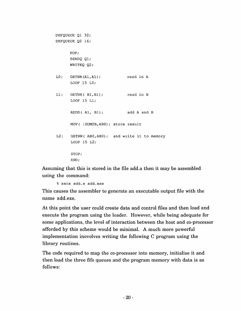
DEFQUEUE Q1 32;
DEFQUEUE Q2 16;
NOP ;
READQ Q1;
WRITEQ Q2;
LO : GETNR (Al, A1 ) ;
LOOP 15 LO;
L1: GETNR( B1,Bl);
LOOP 15 L1;
read i n A
read i n B
ADDD( All Bl); add A and B
MOV ( : SUM2BrABO) ; s t o r e r e s u l t
L2: GETNW( AB0,ABO); and w r i t e it t o memory
LOOP 15 L2;
STOP ;
END ;
Assuming that this is stored in the file add.a then it may be assembled using the command:
% x s c s add.a add.exe
This causes the assembler t o generate an executable output file with the name add.exe.
At this point the user could create data and control files and then load and execute the program using the loader. However, while being adequate for some applications, the level of interaction between the host and co-processor afforded by this scheme would be minimal. A much more powerful implementation inovolves writing the following C program using the library routines.
The code required t o map the co-processor into memory, initialise it and then load the three fifo queues and the program memory with data is as follows:
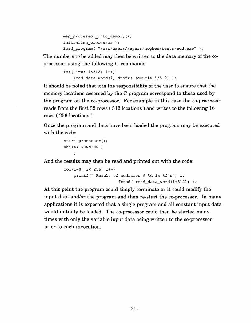
The numbers to be added may then be written to the data memory of the co- processor using the following C commands:
for( i=O; i<512; i++)
load-data-word(i, dtofx( (double) i/512) ) ;
It should be noted that it is the responsibility of the user to ensure that the
memory locations accessed by the C program correspond to those used by the program on the co-processor. For example in this case the co-processor reads from the first 32 rows ( 512 locations ) and writes t o the following 16 rows ( 256 locations ).
Once the program and data have been loaded the program may be executed with the code:
start~rocessor 0 ;
while ( RUNNING )
t
And the results may then be read and printed out with the code:
for(i=O; i< 256; i++)
printf(" Result of addition # %d is %f\nm, i,
fxtod( read-data-word(i+512)) ) ;
At this point the program could simply terminate or it could modify the
input data andlor the program and then re-start the co-processor. In many
applications it is expected that a single program and all constant input data
would initially be loaded. The co-processor could then be started many times with only the variable input data being written to the co-processor prior to each invocation.
4. Writing Software for the Hughes Processor
4.1 Overview
Perhaps the most difficult aspect of the software development process is the determination of a suitable implementation. In the traditional systolic architecture the hardware is a direct implementation of the chosen algorithm [7]. This means that the engineer can effectively start each design with a blank sheet of paper - the constraints on the design imposed
by hardware considerations being only limited by what is physically realisable. The disadvantage with this method is that each design requires specialised hardware which, once created, is difficult to modify or adapt to other problems. The Hughes processor seeks to overcome this limitation by employing a programmable system where there is software control over the implemented function. Unfortunately this additional flexibility does not come without cost and the catch is that it is a non-trivial process to map existing algorithms t o a fixed hardware structure.
The array may be used in a number of different logical configurations. One possibility is t o simulate a systolic architecture with each processing
element performing the tasks of one component in that design. The advantage of this is that data may be processed continuously as it moves through the array. ( In some cases data transfer can be performed in parallel with multiplication or division operations - thus i/o can be
performed with no time penalty.) The disadvantage is that the systolic architecture being implemented may not map well on to the 16x16 processor array. There may also be some loss in parallelism if different components
of the array are required to perform different tasks since in this case some masking of the array would almost certainly be required. It may also be necessary to artificially introduce delays into the system in order to have all the multiplications/ divisions occurring simultaneously.
7 Kung, H.T., 'Why Systolic Architectures", IEEE Computer, Jan, 1982, pp37-46.
An alternative is to treat the array as a SIMD ( single-instruction multiple- data ) machine with 256 parallel processors. This implementation is
particularly efficient since all the processors are busy all the time. The
disadvantage is that some time may be wasted transferring data into, and results out of, the array - though this is mitigated t o a certain extent by the extremely high bandwidth connection between the array and data memory.
Another possibility is t o treat the array as sixteen parallel pipelines ( or one- dimensional systolic machines ). It would even be possible, though not particularly efficient, to use the array t o simulate a 256-stage linear array.
4.2 Opthising the code
When composing code for the processor it is possible to take account of optimisations as the code is written however the resulting code is difficult to read and debug. An alternative method is t o write the code without considering any optimisations and then wait until a working version exists before attempting any improvements. This however has the disadvantage that substantial changes to the coding may be necessary in order to realize relatively minor speed improvements. It was found in practice that a combination of the above two techniques usually produced the best results in terms of both programming and execution time.
There are two main levels at which improvements can be achieved. At the higher level there are global efficiency considerations ( such as the average time each processing element spends performing useful work ). Improvements at this level generally require the selection of an alternative algorithm which maps more cleanly onto the fixed array.
At the lower level it is possible t o achieve some speed improvement by optimising the coding of the algorithm. There are three main areas where these gains can be realised:
Firstly, the use of static registers for temporary storage of results can be
minimised by making use of the fact that the dynamic output registers within each functional unit can be used directly as inputs for successive operations.
Secondly, the use of multiplication and division operations may be optimised by rearranging equations to minirnise the number of divisions and, wherever possible, t o allow two multiplications to be performed in
parallel.
Thirdly, it is often possible to replace the NOP instructions performed during multiplication and division operations by instructions which perform useful work. It should be noted that the dynamic output registers for these operations do not need to be read as soon as the results are available and so it is possible to replace NOPs by instructions which may take slightly longer to execute.

5. Dewription of the Square Root Routine
The aim of this section is t o present an efficient algorithm for determining
square roots using the processing element in the Hughes systolic array co-processor.
It is possible to calculate the square root of any number by hand using a method similar to long division. This manual method can be readily translated into a binary format with the resulting algorithm being particularly well suited t o computer implementation [8]. An alternative
method, described by Johnson [9] is to use a binary search technique to locate the square root. Yet another method is to consider finding the square root of a number to be equivalent to finding the root of the equation flx)=x2-y. This equation may then be solved using an iterative method [lo]. The decision as to which of these alternative methods t o use was effectively pre-determined by the unique hardware design of the processing element. Since each element lacks any conditional, bit-wise, logical o r table-lookup operations the only method which may be implemented efficiently is the iterative solution.
It may be possible to distribute the calculation of a square root across the systolic array ( for example Majithia and Kitai [ll] describe a cellular array
for computing square roots ) however in the present situation it is desirable
8 Cowgill, D., "Logic Equations for a Built-In Square Root Method, IEEE
Transactions on Electronic Computers, April 1964, pp156-157.
9 Johnson, KC., "Algorithm 650: Efficient Square Root Implementation on the
68000n, ACM Transactions on Mathematical Software, Vo1.13, No.2, June, 1987,
~ ~ 1 3 8 - 1 5 1 .
10 Borse, G.J., Fortran 77 and Numerical Methods for Engineers, PWS Engineering,
U.S.4 1985, pp358-361.
11 Majithia, J.C. and Kitai, R., "A Cellular Array for the Nonrestoring Extraction of
Square Roots", IEEE Transactions on Computers, December, 1971, pp1617-1618.
for each processing element to be capable of independently calculating the square root function. Such an implementation allows a large number of square roots to be computed in parallel while simultaneously reducing the amount of communication required between processing elements. This section will therefore consider only the case where a single processing element is required to calculate the square root of a single number.
5.2 Algorithmic Description
For most non-linear functions the computational solution is obtained by some form of non-iterative approximation. However, in the case of the square root function a particularly simple and very fast iterative technique exists. This method is known by various titles including Newton's method and the Newton Raphson method.
Newton's method is a general technique for finding the root of an equation and may be written:
Where xk is the value of x after k iterations ( xo is the initial guess) and f and f are the function and its derivative for which the root is required.
In the case of the square root function:
Clearly this will equal zero only when x = 6 Substituting into (5.1) yields:
Intuitively it seems clear that this iterative formula should always converge ( provided the initial guess is positive) and it has been shown [I21 that this convergence is quadratic.
12 Bajpai A.C., Mustoe L.R. and Walker D., Engineering Mathematics, Wiley, USA, 1982, p352.
Perhaps the most common method for implementing this iterative technique in software is to use the following algorithm:
i) Perform range reduction
ii) Choose an apropriate initial guess.
iii) Solve iteratively until a desired degree of accuracy is obtained
iv) Transform the result to nullify the effects of step (i).
5.3 Range Reduction
If the input numbers are permitted to vary over a very wide range then it becomes difficult t o make an accurate guess as t o the square root of the number. This increases the number of iterations required in step (iii) and consequently slows down the routine. It is therefore common t o reduce the range of the input numbers.
This range reduction is typically performed by shifting the input number by some appropriate number of bits until the input falls within some desired range ( say [1/4,1] ). Such a reduction is particularly easy to nullify after the
square root has been performed since the result can simply be shifted in the reverse direction by half as many places.
The absence of any shift operations makes it difficult t o perform range reduction in this way using the Hughes processor. Even if the shift operations were replaced by multiplication/division operations it is not clear how one could determine which number t o multiplyldivide by and even if this could be determined it would not be easy to nullify the effects of such an operation after the square root had been performed.
Therefore, while there is definitely an advantage to performing range reduction, it is not practical to use it in this implementation. The range of
possible input numbers is therefore [2-30,2). One side effect of this decision is that the choice cf an accurate initial guess becomes even more important.
5.4 Choosing an Initial Guess
Determining a suitable method for finding an initial guess is a compromise between two alternatives. If a very simple method is used ( for example just
using a constant ) then a relatively large number of iterations will be
required. Alternatively, if a more complex method ( for example a 3rd degree polynomial approximation) is used then this will reduce the number of iterations but the savings in iterative calculations may be overshadowed by the increased calculation required for the initial guess. In this case a first-order approximation was considered to provide the best compromise.
There are several alternative methods for determining "optimal" values for the two constants in the first-order approximation. For purposes of comparison consider an approximation for a routine designed to cope with numbers in the range [0.25,1].
5.4.1 Approximation using Mmnnax . . Methods
One way of determining a square root approximation is t o minimise the maximum relative error between the approximation and the square root function.
If the approximation is of the form:
then the relative error is: -
Suitable values for A and B are required in order to minimise:
Solving this using minimax techniques [I31 gives the approximation [14]:
13 Fike, C.T., Computer Evaluation of Mathematical Functions, Prentice Hall,
U.S.A., 1968, pp75-76.
14 Eve, J., "Starting Approximations for the Iterative Calculation of Square Roots", Comput. J., October, 1966, pp274-275.
5.4.2 Approximation using Moursund's Method
Moursund [15] has shown that the above-described result may be improved by considering the relative error after m iterations of Newton's method ( as opposed to the relative error at the output from the approximation step ).
Thus, if Nm(y) is the result after m iterations of Newton's method using a starting approximation of y then values for A and B are required in order t o minimise:
It turns out that the values of A and B remain constant as m increases ( assuming m 2 1 ) and Moursund has tabulated values for a number of different situations. For an input range of [0.25,1] the approximation is:
5.4.3 Approximation using Absolute Error Method
Both of the above two methods aim to minimise relative errors. However, in a computer implementation it is desirable to have a routine which produces answers accurate to the last bit and this implies that it is the absolute, rather than relative, errors which are important.
Hence we require values for A and B which minimise:
m ax ............................................. 0.25s1 I N ~ ~ ( A + B x ) - & \I;; (5.10)
A simple, but computationally intensive, technique for determining the values for A nd B in this equation is to test a number of different values for
15 Moursund, D., "Optimal Starting Values for Newton Raphson Calculation of &", Communications of the A.C.M., Vol.10, No.?, July, 1967, pp430-432.
A and B until a suitable result is obtained [16]. In essence the algorithm is
as follows:
(i) Step A through a range of values
(ii ) Step B through a range of values
(iii ) Determine an approximate value for:
by testing the procedure at discrete values of x.
(iv> If the absolute error for this choice of A and B is lower than the best known then remember these values.
V) Output the values for A and B which produced the lowest absolute error.
It should be noted that in this case the "optimal" values will change as the number of iterations is altered. Approximate values for A and B using the above method are:
P(x) = 0.3486 + 0.6766 x ( for m=l )
P(x) = 0.3459 + 0.6816 x ( for m=2 )
This method only produces approximate answers for A and B since it only tests at discrete points. Nevertheless it produces values which appear to perform better than either of the two alternative methods ( in terms of absolute accuracy of the final result ).
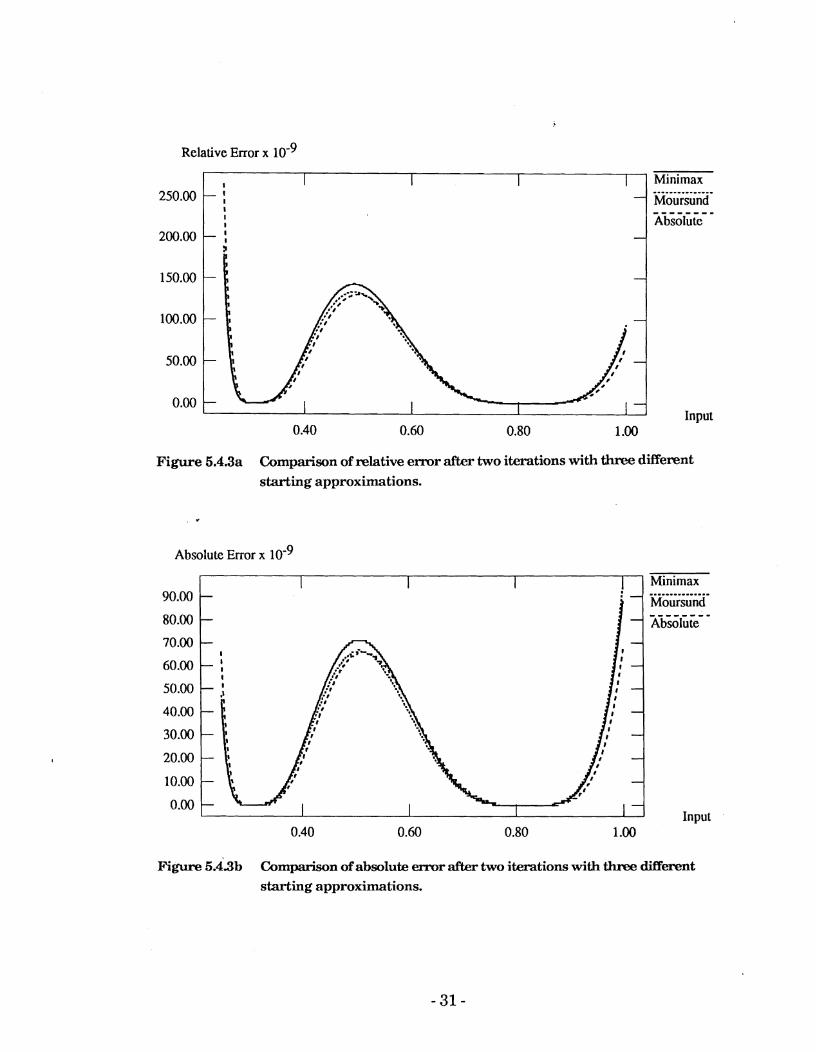
A comparison of the three methods is shown in Figures 5.4.3a and 5.4.3b.
16 This is similar to the technique used by Andrews [ Andrews, M., "Mathematical Microprocessor Software: A & Comparison", IEEE Micro, May, 1982, pp63-79.1 although in tha t case the numerical precision was much lower and so i t was practical to test every possible input number.
Relative Error x
250.00
200.00
Minimax .-..--------.-- Moursund - - - - - - - - Absolute
Input 1 .oO
Figure 6.4.3a Comparison of relative e m r after two iterations with three different starting approximations.
Absolute Error x
Figure 6.4.3b Comparison of absolute error after two iterations with three different starting approximations.
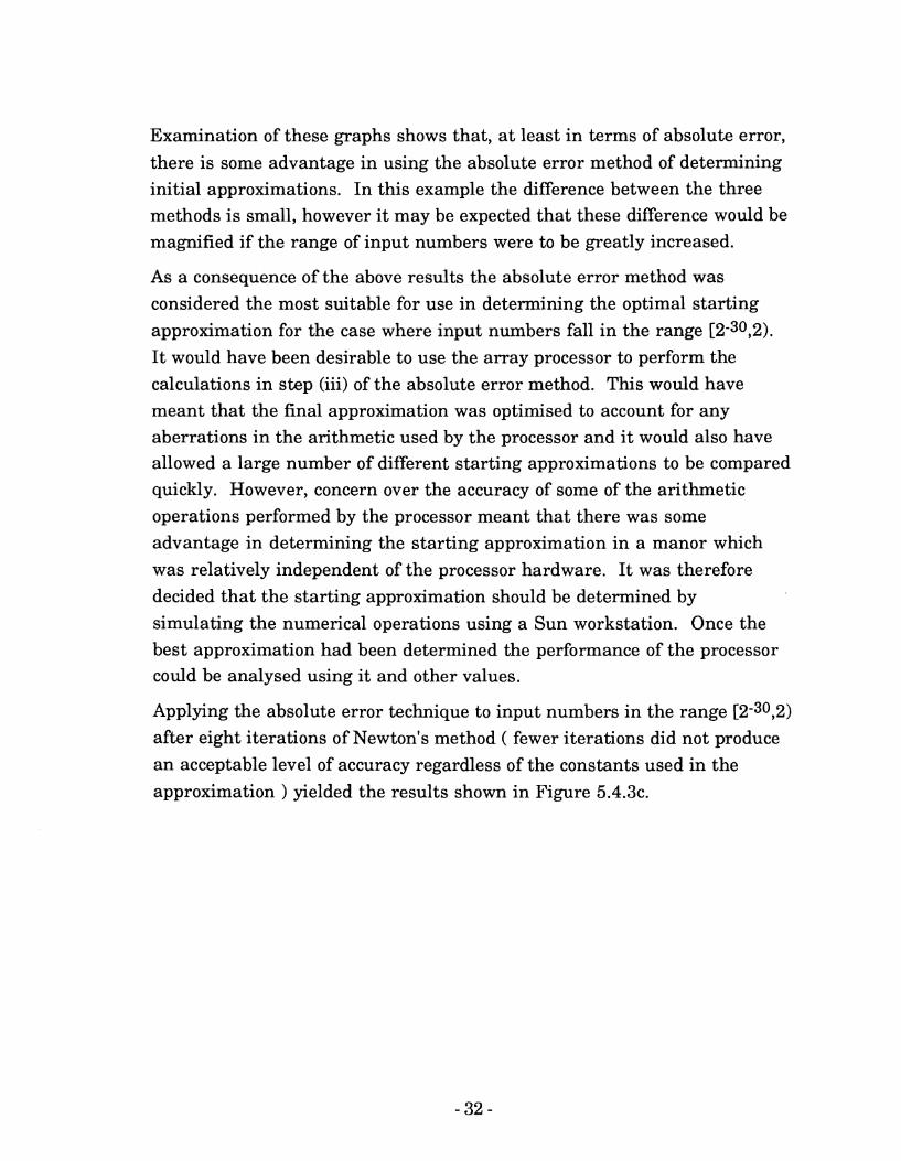
Examination of these graphs shows that, a t least in terms of absolute error,
there is some advantage in using the absolute error method of determining initial approximations. In this example the difference between the three methods is small, however it may be expected that these difference would be magnified if the range of input numbers were t o be greatly increased.
As a consequence of the above results the absolute error method was considered the most suitable for use in determining the optimal starting approximation for the case where input numbers fall in the range [2-30,2).
It would have been desirable to use the array processor to perform the calculations in step (iii) of the absolute error method. This would have meant that the final approximation was optimised to account for any aberrations in the arithmetic used by the processor and it would also have allowed a large number of different starting approximations to be compared quickly. However, concern over the accuracy of some of the arithmetic operations performed by the processor meant that there was some advantage in determining the starting approximation in a manor which
was relatively independent of the processor hardware. It was therefore decided that the starting approximation should be determined by
simulating the numerical operations using a Sun workstation. Once the best approximation had been determined the performance of the processor could be analysed using it and other values.
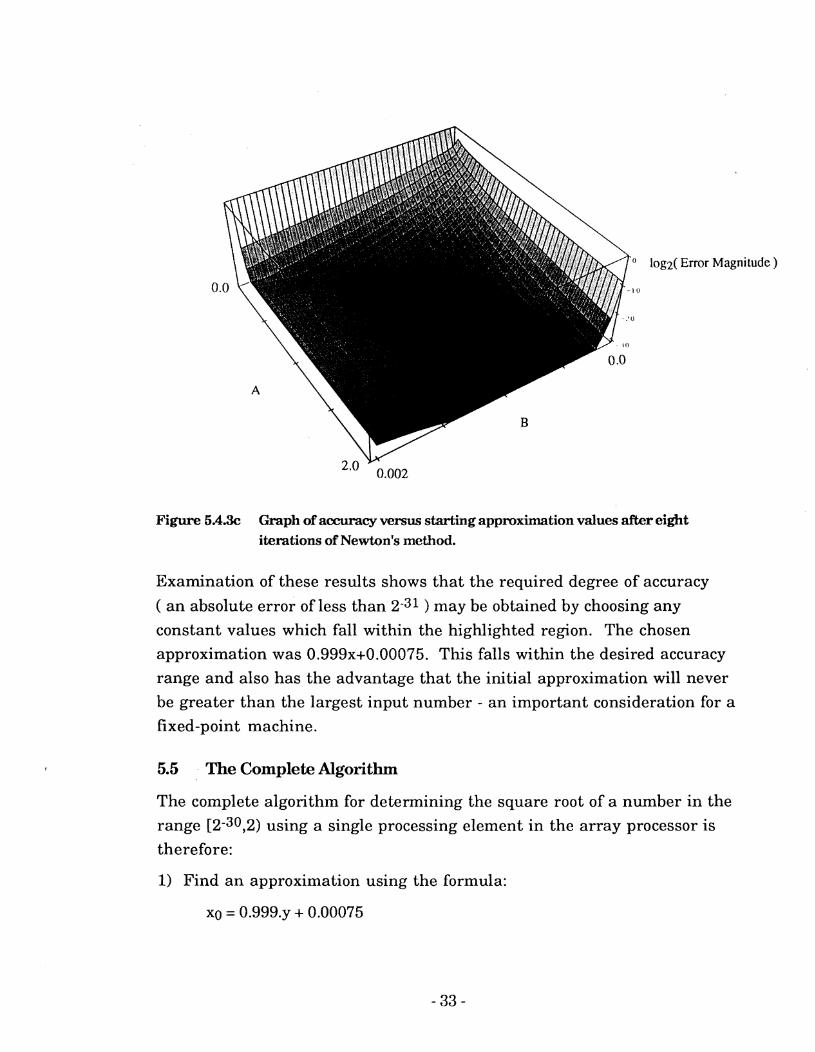
Applying the absolute error technique to input numbers in the range [2-30,2) after eight iterations of Newton's method ( fewer iterations did not produce an acceptable level of accuracy regardless of the constants used in the approximation ) yielded the results shown in Figure 5.4.3~.
log2( Enor Magnitude )
Figure 5.4% Graph of accuracy versus starting approximation values after eight iterations of Newton's method.
Examination of these results shows that the required degree of accuracy
( an absolute error of less than 2-31 ) may be obtained by choosing any
constant values which fall within the highlighted region. The chosen
approximation was 0.999x+0.00075. This falls within the desired accuracy
range and also has the advantage that the initial approximation will never
be greater than the largest input number - an important consideration for a
fixed-point machine.
5.5 The Complete Algorithm
The complete algorithm for determining the square root of a number in the
range [2-30,2) using a single processing element in the array processor is
therefore:
1) Find an approximation using the formula:
2) Perform 8 iterations using the formula:
This algorithm could be translated directly into the machine language for the processor, however the internal architecture of the machine means that some further refinements may be introduced.
Firstly, since division operations take more than twice as long as multiplications, the algorithm may be re-written:
2) templ = y*0.5
3) perform 8 iterations using the formula:
Secondly, the internal parallelism within the processor can be used to
advantage by re-writing the equations as:
1) Perform in parallel: templ = y"0.5 temp2 = 0.9993.
2) temp2 = temp2 + 0.00075
3) Do the following eight times:
temp1 i) Perform in parallel: temp3 = - temp4 = 0.5 * xn Xn
ii) xn+l= temp3+ temp4
The assembly language form for this routine is given in Appendix B.
5.6 Results and Discussion
The above-described routine was tested by using it to calculate the square root of a number of different inputs and the results of this are shown in Figure 5.6.
Error Magnitude x lom6
60.00
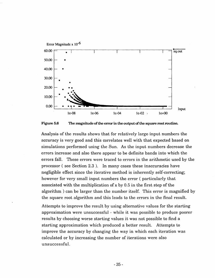
Figure 5.6 The magnitude of the error in the output ofthe s q m mot mutine.
Analysis of the results shows that for relatively large input numbers the
accuracy is very good and this correlates well with that expected based on
simulations performed using the Sun. As the input numbers decrease the
errors increase and also there appear to be definite bands into which the
errors fall. These errors were traced to errors in the arithmetic used by the
processor ( see Section 2.3 ). In many cases these inaccuracies have negligible effect since the iterative method is inherently self-correcting;
however for very small input numbers the error ( particularly that
associated with the multiplication of x by 0.5 in the first step of the
algorithm ) can be larger than the number itself. This error is magnified by the square root algorithm and this leads to the errors in the final result.
C-- sq.out t
Attempts to improve the result by using alternative values for the starting
approximation were unsuccessful - while i t was possible t o produce poorer
results by choosing worse starting values i t was not possible t o find a
starting approximation which produced a better result. Attempts to improve the accuracy by changing the way in which each iteration was
calculated or by increasing the number of iterations were also
unsuccessful.
- . . - . . -
I I 1 - Tnnnt
. - . -
- -
- - . .
I -
6. Dewription of the Sine and Cosine Routine
The aim of this section is to describe the development of a single routine to calculate both the sine and cosine of a given input number. This routine will form the basis for a more complex program described later in the report.
The standard implementation of sine and cosine routines is to perform some range reduction on the data first [17]. The required sinekosine values can then be computed using either a polynomial approximation or table- lookup.
Unfortunately, it is not possible to perform range reduction using the processing element within the Hughes processor. As a result a considerably larger polynomial approximation is required.
6.2 Algorithmic Description
Using Mclaurin's expansion [18]:
It was estimated that truncating this series after the eighth term would provide a reasonable compromise between execution time, register usage and numerical accuracy.
Now, since the machine can't store numbers outside the range [-2,+2) it is
necessary t o perform some scaling of the input values. A scaling factor of .n
provides the elegant result that the input numbers fall within the range
17 Fike, C.T., Computer Evaluation of Mathematical Functions, Prentice Hall,
U.S.A., 1968, p41.
18 Bajpai A.C., Mustoe L.R. and Walker D., Engineering Mathematics, Wiley, USA,
1982, ~~$362-363.
[-l,+l]. Thus, using 'a' as the scaled input value, the series may be formulated as:
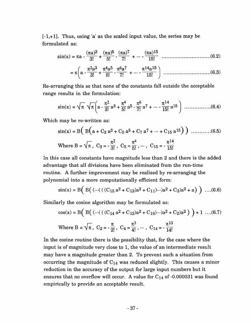
Re-arranging this so that none of the constants fall outside the acceptable range results in the formulation:
Which may be re-written as:
In this case all constants have magnitude less than 2 and there is the added advantage that all divisions have been eliminated from the run-time routine. A further improvement may be realised by re-arranging the polynomial into a more computationally efficient form:
Similarly the cosine algorithm may be formulated as:
cos(x) = B( B( (.-( ( (C14 a2 + C12)a2 + Clo)---)a2 + C2)a2 ) ) + 1 ... i6.7)
In the cosine routine there is the possibility that, for the case where the input is of magnitude very close to 1, the value of an intermediate result
may have a magnitude greater than 2. To prevent such a situation from
occurring the magnitude of Cl4 was reduced slightly. This causes a minor reduction in the accuracy of the output for large input numbers but it ensures that no overflow will occur. A value for C14 of -0.000031 was found empirically to provide an acceptable result.
I t would be possible to calculate the sine and cosine values independently,
however, since each processing element has the ability to perform two
multiplications in parallel there is a considerable advantage to be gained
from interleaving the calculations.
Using eight terms for each series proved to be advantageous in terms of
coding in that it was possible to split the 16 constants between the A and B registers. This left all of the AB registers free for holding input and output
values as well as partial results. Such a mapping allows a number of
sine/cosine pairs to be evaluated without any need to reload the constants
into each processing element.
The resulting code is given in Appendix C.
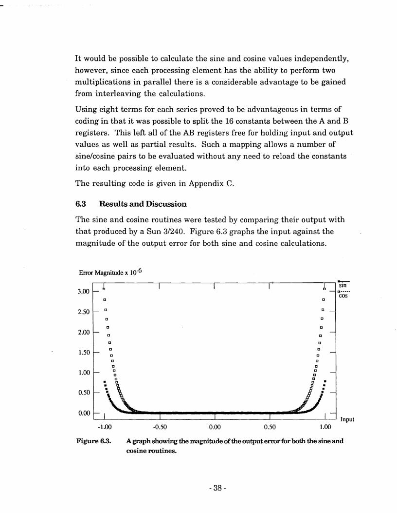
6.3 Results and Discussion
The sine and cosine routines were tested by comparing their output with
that produced by a Sun 31240. Figure 6.3 graphs the input against the
magnitude of the output error for both sine and cosine calculations.
Error Magnitude x loe6
1 .oo
0.50
0.00 Input
3.00
2.50
2.00
1.50
Figure 6.3. A graph showing the magnitude of the output error for both the sine and cosine routines.
I A - - l4
D
-
- - u
- CI, -
_ . sln
m.---- cos
These results indicate a maximum error of magnitude less than 0.000004
which, while being somewhat less than the maximum accuracy possible on the machine, is nevertheless still adequate for the majority of applications.
The difference in accuracy between the sine and cosine results is an artifact of the differing formulae used for each. In the case of the sine routine the eight terms translate to odd powers of x between xl and x15; while in the cosine routine eight terms translates to even powers of x between x* and x14. If an increased accuracy were required then a greater number of terms could be used or alternatively a better polynomial approximation could be developed.
7. Application to Trajectory Planning for Redundant Manipulators.
At present there are a number of areas in Robotics where the computationally-intensive nature of the calculations makes it difficult t o perform real-time evaluation. These include "optimal" trajectory planning,
obstacle avoidance and the control of redundant manipulators [191.
The application of the array co-processor will, in some cases, allow existing algorithms t o be performed more quickly. However, a more significant advantage is that it will enable the application of simpler, but more computationally demanding, solutions.
The aim of this section is to describe the application of the co-processor to one such area - trajectory planning for redundant manipulators.
7.1 Overview
With a two-link planar manipulator it is possible t o determine an inverse kinematics solution directly from a given cartesian end-effector position. However, if a third planar link is added then there are now an infinite number of solutions for many cartesian points within the workspace.
For such a manipulator it is very easy to find a solution but very difficult t o find a "good" solution. Where "good" in this case refers to some desirable feature such as avoiding singularities, dodging objects or minimising travel time.
One possibility, proposed by Yoshikawa [20], is to formulate a solution in
terms of some primary constraint ( for example following a given cartesian trajectory ) and then further restrict that solution by specifying some
19 Zhang, Y., Redundancy Control of a Robot Manipulator using a Systolic Array Processor, PhD Thesis, The Department of Mechanical Engineering and Applied Mechanics, The University of Pennsylvania, 1989.
20 Yoshikawa, T., Foundations of Robotics: Analysis and Control, M.I.T.Press,
England, 1990, pp244-257.
additional constraint ( such as singularity avoidance ). The result of this
task decomposition is a direct formula for the joint velocities.
The method proposed by the author is simpler, but possibly more computationally demanding, than the task decomposition scheme. The system is based on the premise that for many robots it is considerably easier to calculate the forward kinematics solution than it is to find its inverse. It also relies on the fact that, given a joint-space trajectory, it is not too
demanding to find appropriate joint velocities to track that trajectory. Taking these factors into account led to the following algorithm:
i) Given the current position of the robot in joint-space create a set of points to which it could move if each of the joints were moved some
small discrete amount.
ii) For each of these points, calculate a forward kinematics solution. The result of this step is that the system knows a range of positions in cartesian space to which the robot could move.
iii) Eliminate from this set of positions any which lie outside of the desired trajectory path.
iv) Now choose from among the remaining points based on some other criteria such that only a single "best" point remains.
V) That point becomes the next point on the robot's path and the process is repeated from step (i) until the entire trajectory has been followed.
Note that this routine makes no assumption concerning the existence of a direct inverse kinematics solution - it generates a joint-space trajectory from a cartesian space trajectory while only using forward kinematics.
The above-described algorithm is well suited t o a parallel implementation with steps (i)-(iv) all being amenable t o parallel computation. However, taking into account the capabilities of the array processor, it was considered that a more efficient implementation would be to have the array co- processor compute the forward kinematics solutions in step (ii) while the host machine performed the remaining calculations.
The implementation thus decomposed into two separate areas. Firstly a forward kinematics solution had to be implemented using the co-processor
and then the remainder of the algorithm had t o be implemented on the host
machine.
7.2 Implementation on the Co-processor
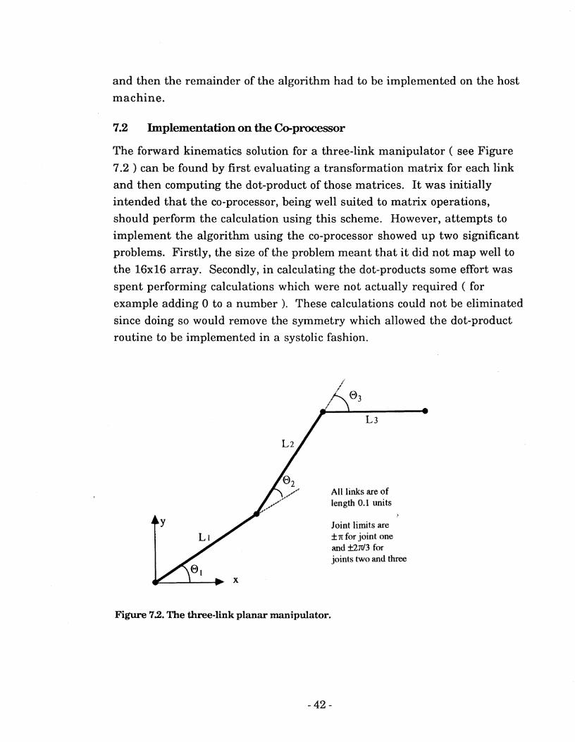
The forward kinematics solution for a three-link manipulator ( see Figure
7.2 ) can be found by first evaluating a transformation matrix for each link and then computing the dot-product of those matrices. I t was initially intended that the co-processor, being well suited t o matrix operations,
should perform the calculation using this scheme. However, attempts t o implement the algorithm using the co-processor showed up two significant
problems. Firstly, the size of the problem meant that it did not map well to
the 16x16 array. Secondly, in calculating the dot-products some effort was
spent performing calculations which were not actually required ( for
example adding 0 to a number ). These calculations could not be eliminated
since doing so would remove the symmetry which allowed the dot-product
routine t o be implemented in a systolic fashion.
All links are of length 0.1 units
Joint limits are f TT for joint one and +2fl3 for joints two and three
Figure 72. The three-link planar manipulator.
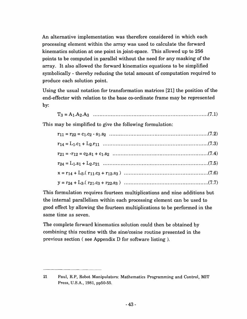
An alternative implementation was therefore considered in which each processing element within the array was used to calculate the forward kinematics solution at one point in joint-space. This allowed up to 256 points to be computed in parallel without the need for any masking of the array. It also allowed the forward kinematics equations to be simplified
symbolically - thereby reducing the total amount of computation required to produce each solution point.
Using the usual notation for transformation matrices [21] the position of the end-effector with relation to the base co-ordinate frame may be represented by:
....................................................................... T3 = A1.A2.A3 (7.1)
This may be simplified to give the following formulation:
This formulation requires fourteen multiplications and nine additions but
the internal parallelism within each processing element can be used to good effect by allowing the fourteen multiplications to be performed in the same time as seven.
The complete forward kinematics solution could then be obtained by combining this routine with the sinelcosine routine presented in the previous section ( see Appendix D for software listing ).
21 Paul, R.P, Robot Manipulators: Mathematics Programming and Control, MIT Press, U.S.A., 1981, pp50-55.
7.3 Implementation on the Host
The host machine is required to select points to which the manipulator
could move from its previous position. This is achieved by varying 81 by some small discrete amount ( in this case five possible values distributed evenly in the range el+ 0.001 radians were used). For each value of 81,82 is
stepped through a range of values in a similar fashion and for each of these points 83 is also varied. The result is a number of possible positions in joint-
space. It was not practical to calculate values for the joint angles using the co-processor due to the necessity of checking for joint limits.
Once suitable values in joint-space have been located they are written to the co-processor and the host need only start the co-processor running and then await the results of the forward kinematics calculations.
After the forward kinematics values have been found it is necessary to select the "best" one. In this case some possible points were first eliminated
based on the criterion that each point on the cartesian trajectory must be within a certain specified distance of a straight-line cartesian path and that it must be closer to the target than the previous point. The remaining
points are then searched to find the one which minimises the cartesian distance between the end-effector and the target point.
While it would have been desirable to implement this search in a parallel manor this was impractical due to the lack of any conditional constructs in the co-processor ( the co-processor does have a sort command which could be used t o find the minimum cartesian distance but there is no way to relate
back from that distance to the point at which it occurred ).
Once the "best" point has been found it becomes the next point along the trajectory and the process is repeated until the end-effector reaches the target point.
7.4 Results and Discussion.
In the first test the system was required to create a trajectory between the cartesian points (0.3,O.O) and (0.0,0.2) with the "best" point at each step in
the algorithm being the one which minimised the cartesian distance. The results of this are shown in Figure 7.4.1.
Examination of this graph shows that initially the motion results from moving all three joints by the maximum amount a t each step - this has the effect of reducing the cartesian distance by the greatest amount a t each step. Toward the end of the trajectory i t is no longer possible to move in this way while satisfying the constraint that the cartesian distance be minimised. As a result joint one is forced to move back t o bring the end- effector t o the final position.
Examination of the changing joint angles shows the interesting result that joints 2 and 3, which both had to move the maximum distance, have moved the maximum amount at each step throughout the entire motion. Thus, given the constraint that each joint can move a maximum of 0.001 radians at each step, the trajectory appears to be optimal in terms of the total number of steps required.
Figure 7.4.2 shows the result of requiring motion between the same two points but applying the constraint that the end-effector must remain within k0.02 units of a straight-line cartesian trajectory.
In this case the arm advances from rest with all three joints moving the
maximum amount a t each step. This is the same as the previous case. However, once the end-effector reaches a point close to +0.02 units from the straight line trajectory further motion in this manor is impossible without violating the straight line constraint. As a result joint one is forced to move back and joint two is slowed down to achieve the desired near straight-line motion.
Examination of the joint angles shows that it is nearly always the case that one of the joints is moving at the maximum amount a t each step.
Comparison of this with the previous motion shows that, as one might expect, considerably more steps were required for the case where the straight line condition was specified.
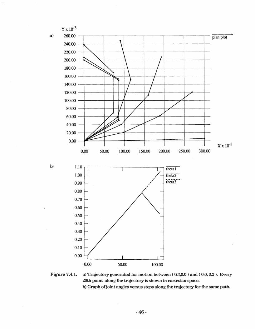
Figure 7.4.1. a) Trqjedory generated for motion between ( 0.3,O.O 1 and ( 0.0,0.2 1. Every 20th point along the trajectory is shown in cartesian space.
b) Graph of joint angles versus steps along t l~e trajectory for the same path.
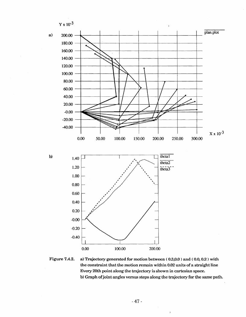
Figure 7.4.2. a) Trqjectory generated for motion between ( 03,O.O ) and ( 0.0,O.Z ) with the constraint that the motion remain within 0.02 units of a straight line Every 20th point along the tmjectory is shown in cartesian space. b) Graph of joint angles versus steps along the trajectmy for the same path.
In the second test the system was required to move between (0.3,O.O) and (-0.3,O.O). Again it was required that points be chosen to minimise the cartesian distance at each step. The resulting trajectory is shown in Figure 5.4.3.
One might expect that the manipulator could move between the initial and
target points using only joint one while joints two and three remained stationary. However, while this would accomplish the same end result the intermediate points along the trajectory would be further way from the target point than in this generated trajectory. This system therefore appears to offer some advantage over moving along a straight line in joint- space.
The trajectory is sub-optimal ( in terms of the total number of steps required ). This appears to be the result of excessive motion by joint three.
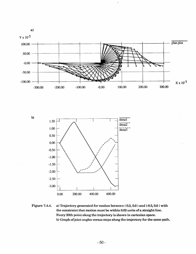
Figure 7.4.4 shows motion between the same points but with the additional constraint that the end-effector remain within k0.02 of a straight line cartesian trajectory. This is a more difficult task due to the need to pass close to the origin.
As for the previous case there is the predictable result that considerably more steps are required to specify the trajectory when straight-line motion is required.
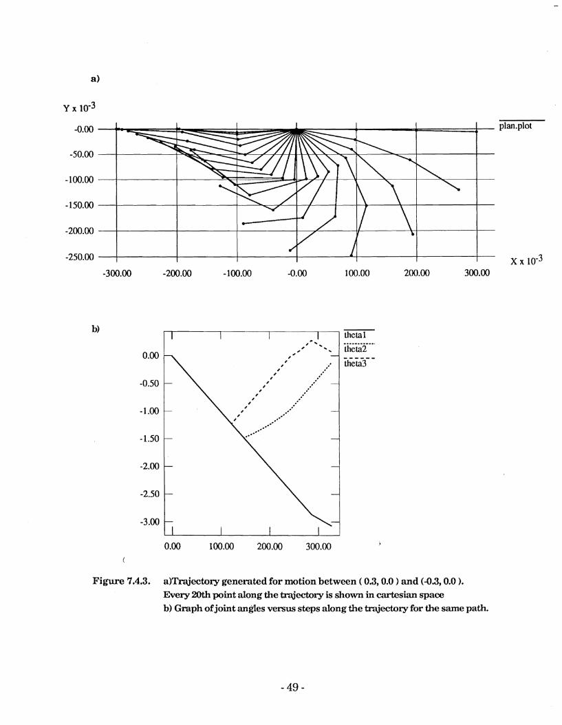
Figure 7.4.3. a)Trajectory generated for motion between ( 0.3,O.O and (-0.3,O.O ). Every 20th point along the trqjedory is shown in cartesian space b) Graph of joint angles versus steps along the trajectory for the same path.
- -I I 1 theta1 ............
the ta2 - --- - - -
theta3 -
I \ 4 \
I .
\ \
- \ \ \ \
- \ \
\-'. ...............-. -
-
I
Figure 7.4.4. a) Trajectory generated for motion between ( O.3,O.O ) and (-0.3,O.O ) with the constraint that motion must be within 0.02 units of a straight line. Every 20th point along the trajectory is shown in cartesian space. b) Graph of joint angles versus steps along the trajectory for the same path.
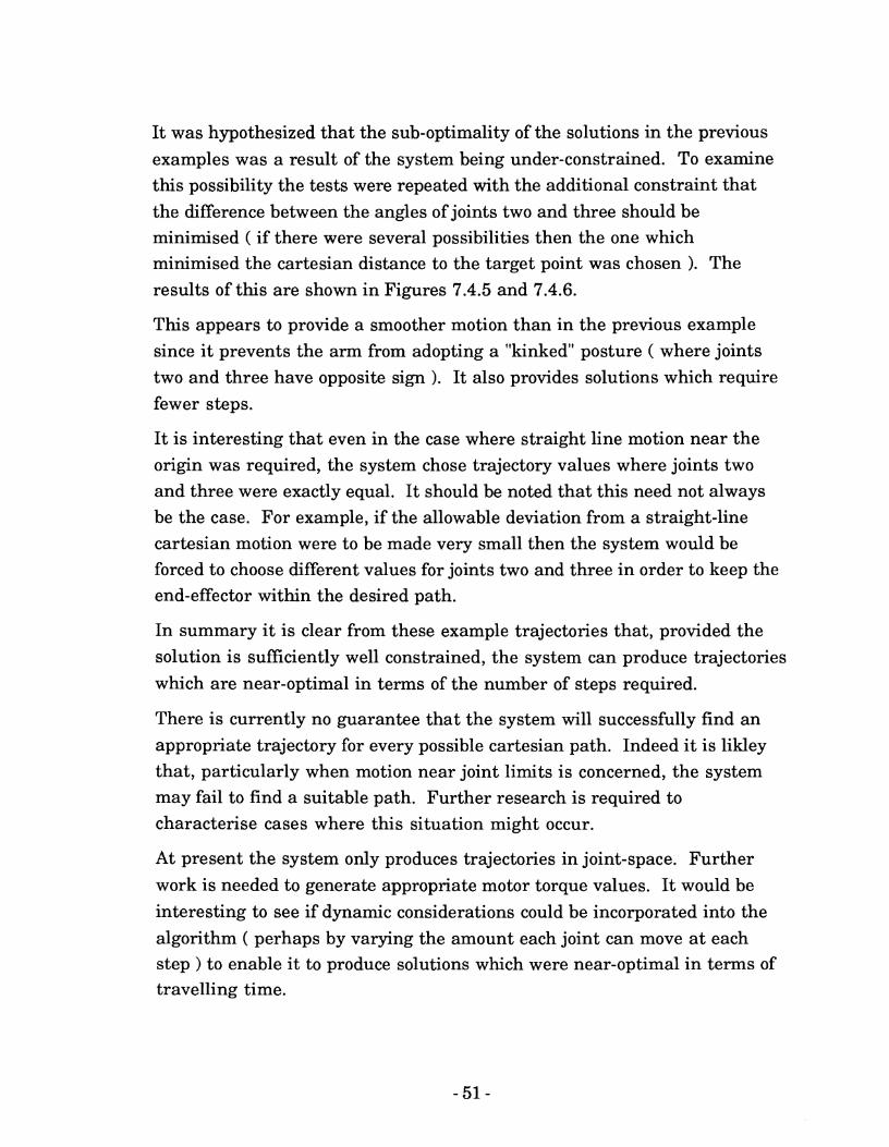
It was hypothesized that the sub-optimality of the solutions in the previous examples was a result of the system being under-constrained. To examine
this possibility the tests were repeated with the additional constraint that the difference between the angles of joints two and three should be minimised ( if there were several possibilities then the one which minimised the cartesian distance to the target point was chosen ). The
results of this are shown in Figures 7.4.5 and 7.4.6.
This appears t o provide a smoother motion than in the previous example since it prevents the arm from adopting a "kinked" posture ( where joints
two and three have opposite sign ). It also provides solutions which require fewer steps.
It is interesting that even in the case where straight line motion near the origin was required, the system chose trajectory values where joints two and three were exactly equal. It should be noted that this need not always be the case. For example, if the allowable deviation from a straight-line cartesian motion were to be made very small then the system would be forced to choose different values for joints two and three in order to keep the end-effector within the desired path.
In summary it is clear from these example trajectories that, provided the solution is sufficiently well constrained, the system can produce trajectories
which are near-optimal in terms of the number of steps required.
There is currently no guarantee that the system will successfully find an appropriate trajectory for every possible cartesian path. Indeed it is likley that, particularly when motion near joint limits is concerned, the system may fail to find a suitable path. Further research is required to characterise cases where this situation might occur.
At present the system only produces trajectories in joint-space. Further
work is needed to generate appropriate motor torque values. It would be interesting to see if dynamic considerations could be incorporated into the algorithm ( perhaps by varying the amount each joint can move at each step ) t o enable it to produce solutions which were near-optimal in terms of travelling time.
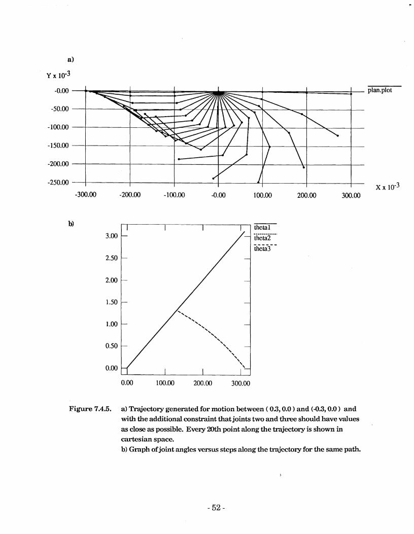
Figure 7.4.5. a) Traijectory generated for motion between ( 03,O.O ) and (-0.3,O.O and with the additional constraint that joints two and three should have values as close as possible. Every 20th point along the m'ectory is shown in cartesian space. b) Graph of joint angles versus steps along the trajectory for the same path.
Figure 7.4.6. a) Trajectory generated for motion between ( 0.3,O.O ) and (-0.3,O.O ) with the constraint that motion must be within 0.02 units of a straight line and with the additional constraint that joints two and three should have values as close as possible. Every 20th point along the trajectory is shown in cartesian space. b) Graph ofjoint angles versus steps along the trajectory for the same path.
8. Discussion and Suggested Design Modi.fications
This section presents a discussion of some suggested changes for future hardware designs as well as some desirable features for future software implementations.
8.1 Hardware
The current implementation of the processor only supports fixed-point operations. The result is that considerable time must be spent examining every algorithm to ensure that no input, intermediate or final value exceeds the storage capability of the machine. In the case of complicated algorithms this is a non-trivial task. It is recommended that future implementations employ a floating-point format ( this has previously been suggested by Zhang[22] ).
At present the processing elements only support the four basic arithmetic operations and a sort function. The incorporation of additional functions ( for example bitwise operations) would increase the number of situations in which the co-processor could be utilized.
The sort function in each processing element went some way towards reducing the problem posed by the lack of conditional statements. However, while the sorter can be used to find the maximum/minimum of two
numbers it can not indicate which was the largerhmaller. What is needed is a combined sort/move operation which sorts two registers and then swaps the contents of two other registers if, and only if, the numbers to be sorted were in ascending order.
Such a function would be particularly useful for implementing code of the form:
22 Zhang, Y., Redundancy Control of a Robot Manipulator using a Systolic Array Processor, PhD Thesis, The Department of Mechanical Engineering and Applied Mechanics, The University of Pennsylvania, 1989, p87.
i f ( x < TOLLERANCE )
y = 0;
else
y = f ( x )
Since this could be implemented as:
S t o r e 0 i n register BO
C o m p u t e f ( x ) and store i n register A0
S o r t ( x,TOLLERANCE ) and s w a p A0 and BO i f f x < TOLLERANCE
T h i s leaves t h e r e s u l t i n AO.
Note that by use of such a hnction several instances which would otherwise have required iflthen type constructs could be implemented.
Another possibility is to provide support for conditional operations in a similar way to that used in early IBM programming languages ( and presumably replicated in hardware ). The basic idea was to have comparison operations setlclear indicator bits. For example: " compare b and c and set indicator 43 iff b=c". Subsequent operations could then be predicated on combinations of these bits. For example: "perform the following operation iff indicator 12 is clear and indicator 87 is set". Such a scheme would seem to be well suited to a parallel implementation. A single
register within each processing element could be used to store up to 32 indicator bits and these could then be setlreset/tested using standard bitwise operations. Each processing element could compare its indicator bits t o a programmable register and thereby decide whether or not to perform the current instruction.
If this system of indicator bits were implemented then it may be possible to remove the necessity of specifying a 32-bit mask field within each instruction. For example, consider the case where an additional register
were provided within each processing element which, when read, returned
the unique position of that element within the array. Each processing element could then use this information in conjunction with input data to
set/clear its own indicator bits during program execution. By predicating subsequent operations on those bits any possible combination of processing elements could be enabled.
At present it is not possible to create an on-line debugger for the Hughes
processor. While it would be possible to write a program on the host which single-stepped the co-processor, there is currently no way t o print out the internal status of each processing element ( the dynamic registers would decay long before they could be read ). One possible solution would be to implement the output registers within each functional unit as static registers. This would not only make de-bugging easier it would also remove the restriction that results must be used within a short time of their computation.
8.2.1 The Assembler
The assembler performed well during testing however there were a few additional features which would have been desirable:
Some form of improved error-checking would be helpful. For example it would be useful t o have warnings for cases where dynamic registers are read after their contents have decayed or before their contents have been fully computed ( this has previously been suggested by Hartholtz [231 ).
Some support for nested loops would also be helpful although this would be complicated to implement due t o the way program memory addresses are
handled in hardware.
It is particularly difficult to write code at the assembler level due to the number of factors which must constantly be kept in mind. The result is that one tends to become overwhelmed with the details of programming and the overall algorithm becomes lost in the static. Some higher-level form of
programming the processor would be of great benefit. For example a program which could convert a series of arithmetic expressions into optimised assembly language t o run on a processing element would be particularly helpful.
23 Hartholz, M.A., The Systolic/Cellular System Assembler: User's Guide, Master's Thesis, The University of Pennsylvania, August, 1988, p95.
8.2.2 The Simulator
During testing of the simulator the author found that virtually every desirable feature was already included.
The only significant difficulty found in practice was that the simulator did not give exactly the same mathematical results as the co-processor. However, since the differences were due primarily to the limited accuracy of the co-processor it is difficult to see how such a feature could be implemented.
8.2.3 The Run time system
At present the loader program and the library of C functions only support the use of the processor with one program at a time. Since the size of the average program is considerably smaller than the program memory there is some justification for considering the possibility of having several programs resident in memory simultaneously. It is possible that such a scheme could be implemented although it would be a non-trivial process due to the need to re-map the addresses in the fifo queues.
9. Conclusions
A loader program and library of C-callable routines have been developed and tested. The loader program was effective in the testing of simple programs while the library of C-callable routines was used successfully in
the development of systems which required a significant level of interaction between the co-processor and the host machine.
Routines to compute square root, sine and cosine functions using the array co-processor have been created and their performance has been evaluated. The implementation of these routines was complicated by the inability of the co-processor to perform range reduction on the input. It was found that the accuracy of the square root routine was limited by errors in the arithmetic
used by the co-processor; while the accuracy of the sine and cosine functions was limited by the form of polynomial approximation employed.
A trajectory planning algorithm for redundant manipulators has been implemented. This algorithm generates a joint space trajectory from a cartesian space trajectory by using the co-processor to compute in parallel a large number of forward kinematics solutions. The system was tested using a three-link planar manipulator and it was found to provide solutions which were near-optimal ( in terms of the number of trajectory points required for each planned path ).
While implementing the forward kinematics solution on the co-processor it was found that considerable efficiency gains could be realised by treating the array as a SIMD machine rather than as a systolic array.
The hardware and software have been analysed and a number of recommendations have been made concerning both future hardware implementations and improvements to the existing software.
Appendix A - The Testing Process.
Some time was spent in the initial phases of this research in testing and debugging the existing hardware and software. At the time this research was started the assembler had only been used in conjunction with the simulator and the first stage of the testing process was therefore to develop a loader program which could take the assembler output and execute it on the array co-processor. This program has wider application than just within the testing process and is described more fully within the main body
of the report.
Once the loader program was written the assembled loader/ hardware combination was tested by writing assembly language versions of routines used in the pre-existing hardware test programs. These routines could then be assembled, loaded and executed; with the results being compared t o those produced by the existing test programs.
This process was complicated by the fact that there were errors in the assembler, loader, co-processor hardware and original test programs.
These errors are perhaps to be expected given the complexity of the systems involved.
The only error found with the assembler was that the phase one and phase two instruction op-codes were reversed in the output file. This was corrected by reversing the phases in the loader program.
Errors in the loader program were largely a result of misunderstandings concerning the detailed operation of the hardware and these were corrected with reference to the pre-existing test routines.
Errors in the co-processor hardware proved particularly difficult to characterise. The symptoms being that the machine would produce incorrect mathematical results when certain input data was used, but correct results when different inputs were employed. These problems were traced to deficiencies in the processing elements and were largely corrected by slowing the system clocks. The author is indebted to Charles Martin for his assistance in this regard.
One side-effect of this change in speed is that multiplication and division operations now require fewer instruction cycles. Only three NOP ( o r equivalent length ) instructions are now needed during multiplication and only ten are required during division.
At the present time all known bugs have been removed from the software development system. Most of the significant errors in the hardware have also been corrected although some inaccuracy is still present in the multiplier and divider units ( see Section 2.3 ).
Appendix B - Software for the Square Root Routine
P r o g r a m - s q u a r e - r o 0 t . a
A u t h o r - C r a i g S a y e r s
D a t e - 3 N o v 1 9 9 0
P u r p o s e - T h i s p r o g r a m c a l c u l a t e s t h e s q u a r e root of a n u m b e r
u s i n g a n i n i t i a l l i n e a r a p p r o x i m a t i o n a n d t h e n
i m p r o v i n g t h a t b y t h e u s e of 8 i t t e r a t i o n s o f
N e w t o n ' s m e t h o d .
i R e g i s t e r M a p :
A 0 N, t h e n u m b e r t o be square- rooted .
B 0 C o n s t a n t A
B 1 C o n s t a n t B, i n i t i a l a p p r o x = A . N + B
ABO C o n s t a n t 0 . 5
A B 1 T e m p o r a r y storage a n d f i n a l r e s u l t
AB2 T e m p o r a r y s to rage
DEFQUEUE Q 1 64 ;
DEFQUEUE Q 2 1 6 ;
NOP;
READQ Q 1 ;
WRITEQ Q 2 ;
LO: G E T N R ( BO, BO) ;
LOOP 15 LO:
L 1 : G E T N R ( B 1 , B l ) ;
LOOP 15 L 1 ;
L 2 : GETNR ( ABO, ABO) ;
LOOP 15 L 2 ;
L 3 : GETNR ( AO, AO) ;
LOOP 1 5 L 3 ;
C o n s t a n t s a n d i n p u t n u m b e r s
O u t p u t N u m b e r s
R e a d i n A c o n s t a n t s
R e a d i n B c o n s t a n t s
R e a d i n 0 . 5 c o n s t a n t s
R e a d i n v a l u e s f o r N
{------- GENERATE I N I T I A L APPROXIMATION ------I
MULTFD( A 0 , B O : A0,ABO ) ; { P R O D l A = N*A : PROD2B = N * 0 . 5 )
NOP;
NOP;
NOP;
NOP ;
NOP ;
MULTSD;
A D D 2 ( P R O D l A , B1 ! ; { SUM2B = N*A + B )
MOV( : SUMZB, AB2 ) ; { AB2 = f i r s t - g u e s s
( - - - - - - F I R S T I T E R A T I V E S T E P ------I
D I V F ( AB2, A B 1 ) ;
D I V S ;
NOP;
MULTF2 ( ABO, AB2 ) ;
NOP ;
NOP;
NOP;
NOP;
NOP ;
MULTS2 ;
NOP;
NOP;
NOP ;
NOP;
{ -+- QUOTA = N * 0 . 5 / f i r s t - g u e s s )
I I I I
( I -+- PROD2B = 0 . 5 * f i r s t - g u e s s 1
{ I I }
{ I I )
{ I I I { I I 1
{ I I
{ I - / )
I I I I ( I t -1 I
ADD2 ( QUOTA, PRODZB) ; { SUM2B = f i r s t p u e s s * 0 . 5 + N * 0 . 5 / f i r s t - g u e s s )
MOV( : SUMZB, AB2 ) ; { AB2 = n e w r e s u l t )
{ - - - - - - SECOND I T E R A T I V E S T E P - - - - - - )
D I V F ( AB2, A B 1 1;
D I V S ;
NOP ;
MULTF2 ( ABO, AB2 ! ; NOP;
NOP ;
NOP;
NOP;
NOP;
MULTSZ;
NOP;
NOP;
NOP;
NOP;
QUOTA = N * 0 . 5 / r e s u l t
ADD2 ( QUOTA, PROD2B) ; { SUM2B = r e s u l t * 0 . 5 + N * 0 . 5 / r e s u l t )
MOV( : SUM2B, AB2 ) ; { AB2 = n e w r e s u l t 1
{------ T H I R D I T E R A T I V E S T E P ------I
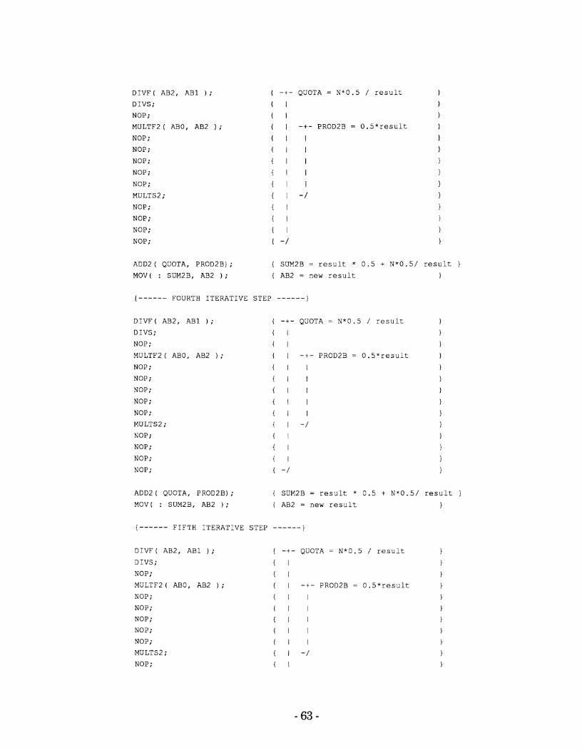
D I V F ( AB2, A B 1 ) ;
D I V S ;
NOP;
MULTF2 ( ABO, AB2 ) ;
NOP ;
NOP ;
NOP;
NOP;
NOP;
MULTS2;
NOP;
NOP ;
NOP;
NOP ;
QUOTA = N * 0 . 5 / r e s u l t
ADD2 ( QUOTA, PROD2B) ; { SUM2B = r e s u l t * 0 . 5 + N * 0 . 5 / r e s u l t )
MOV ( : SUM2B, AB2 ) ; { AB2 = new r e s u l t )
( - - - - - - FOURTH I T E R A T I V E S T E P - - - - - - )
D I V F ( A B 2 , A B 1 ) ;
D I V S ;
NOP;
MULTF2 ( ABO, AB2 ) ;
NOP ;
NOP ;
NOP;
NOP;
NOP ;
MULTSZ;
NOP;
NOP;
NOP;
NOP ;
i -+- QUOTA = N * 0 . 5 / r e s u l t
i I
i I ( I -+- PRODZB = 0 . 5 * r e s u l t
i 1 I i l I
I I { I I ( I I
i I -/ I
i I ( I
( -1
ADD2 ( QUOTA, PROD2B) ; { SUM2B = r e s u l t * 0 . 5 + N * 0 . 5 / r e s u l t )
MOV( : SUMZB, AB2 ) ; ( AB2 = new r e s u l t 1
{ - - - - - - F I F T H I T E R A T I V E S T E P - - - - - - )
D I V F ( AB2, A B 1 ;
D I V S ;
NOP;
MULTF2 ( ABO, AB2 ) ;
NOP ;
NOP;
NOP;
NOP;
NOP;
MULTS2;
NOP;
QUOTA = N * 0 . 5 / r e s u l t 1
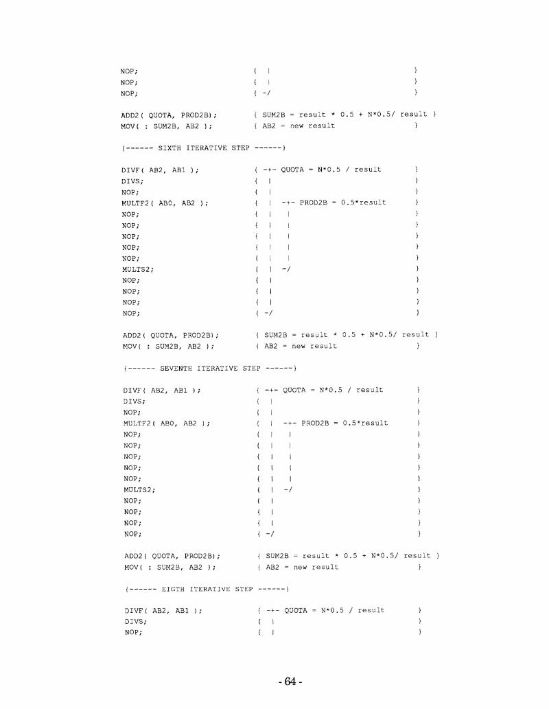
NOP;
NOP;
NOP;
ADD2 ( QUOTA, PROD2B) ; { SUM2B = r e s u l t * 0 . 5 + N * 0 . 5 / r e s u l t )
MOV( : SUM2B, AB2 ) ; ( AB2 = n e w r e s u l t )
(------ S I X T H I T E R A T I V E S T E P ------)
DIVE'( AB2, A B 1 ) ;
D I V S ;
NOP;
MULTF2 ( ABO, AB2 ) ;
NOP;
NOP;
NOP;
NOP;
NOP ;
MULTS2;
NOP ;
NOP;
NOP ;
NOP;
{ -+- QUOTA = N * 0 . 5 / r e s u l t
{ I I I ( I -+- PROD2B = 0 . 5 * r e s u l t
( I 1
( I I
{ I I
( I I
{ I I
I I - /
( I
{ I
( I
( - /
ADD2 ( QUOTA, PROD2B) ; ( SUM2B = r e s u l t * 0 . 5 + N * 0 . 5 / r e s u l t I
MOV( : SUMZB, AB2 ) ; { AB2 = n e w r e s u l t )
{ - - - - - - SEVENTH I T E R A T I V E S T E P - - - - - - )
D I V F ( AB2, A B 1 ) ;
D I V S ;
NOP ;
MULTF2 ( ABO, AB2 ;
NOP;
NOP;
NOP;
NOP ;
NOP;
MULTS2;
NOP;
NOP;
NOP ;
NOP ;
{ -+- QUOTA = N * 0 . 5 / r e s u l t
( I
( I { I -+- PROD2B = 0 . 5 * r e s u l t
( 1 I
( I 1 { I I
( I I
{ I I
( I - / ( I
( I
I
( -1
ADD2 ( QUOTA, PROD2B) ; { SUM2B = r e s u l t * 0 . 5 + N * 0 . 5 / r e s u l t )
MOV( : SUM2B, AB2 ) ; { AB2 = n e w r e s u l t
{ - - - - - - E I G T H I T E R A T I V E S T E P ------I
D I V F ( A B 2 , AB1 ) ; { -t- QUOTA = N * 0 . 5 / r e s u l t )
D I V S ; ( I }
NOP; { I
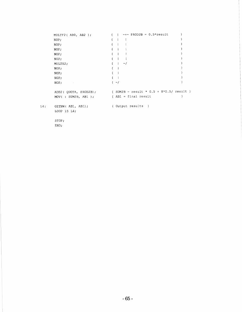
MULTF2 ( ABO, AB2 ) ;
NOP;
NOP;
NOP;
NOP;
NOP;
MULTS2 ;
NOP ;
NOP;
NOP ;
NOP;
ADD2 ( QUOTA, PRODZB) ;
MOV( : SUMZB, A B 1 ) ;
L 4 : GETNW( A B l , A B 1 ) ;
LOOP 15 L 4 ;
{ SUMZB = r e s u l t * 0 . 5 + N * 0 . 5 / r e s u l t 1 ( AB1 = f i n a l r e s u l t )
{ O u t p u t r e s u l t s 1
STOP;
END;
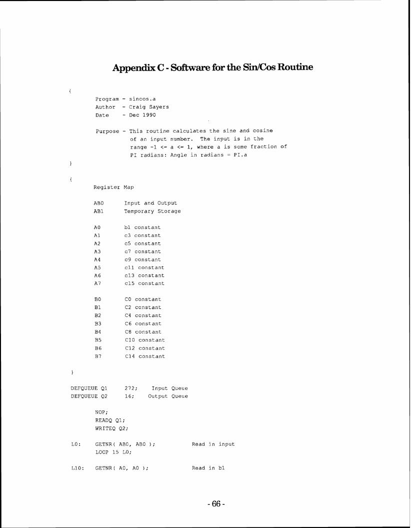
Appendix C - Software for the W C o s Routine
P r o g r a m - s i n c 0 s . a
A u t h o r - C r a i g S a y e r s
D a t e - D e c 1 9 9 0
P u r p o s e - T h i s r o u t i n e c a l c u l a t e s t h e s i n e a n d c o s i n e
o f a n i n p u t n u m b e r . T h e i n p u t i s i n t h e
r a n g e -1 <= a <= 1, w h e r e a i s s o m e f r a c t i o n o f
P I r a d i a n s : A n g l e i n r a d i a n s = P 1 . a
R e g i s t e r Map
ABO I n p u t a n d O u t p u t
AB1 T e m p o r a r y S t o r a g e
DEFQUEUE Q 1
DEFQUEUE 0 2
b l c o n s t a n t
c 3 c o n s t a n t
c 5 c o n s t a n t
c 7 c o n s t a n t
c 9 c o n s t a n t
c l l c o n s t a n t
c 1 3 c o n s t a n t
c 1 5 c o n s t a n t
CO c o n s t a n t
C2 c o n s t a n t
C 4 c o n s t a n t
C6 c o n s t a n t
C8 c o n s t a n t
C10 c o n s t a n t
C12 c o n s t a n t
C14 c o n s t a n t
NOP;
READQ Q1;
WRITEQ Q2;
2 7 2 ; I n p u t Q u e u e
1 6 ; O u t p u t Q u e u e
L O : GETNR ( ABO, ABO ) ;
LOOP 1 5 LO;
R e a d i n i n p u t
R e a d i n b l
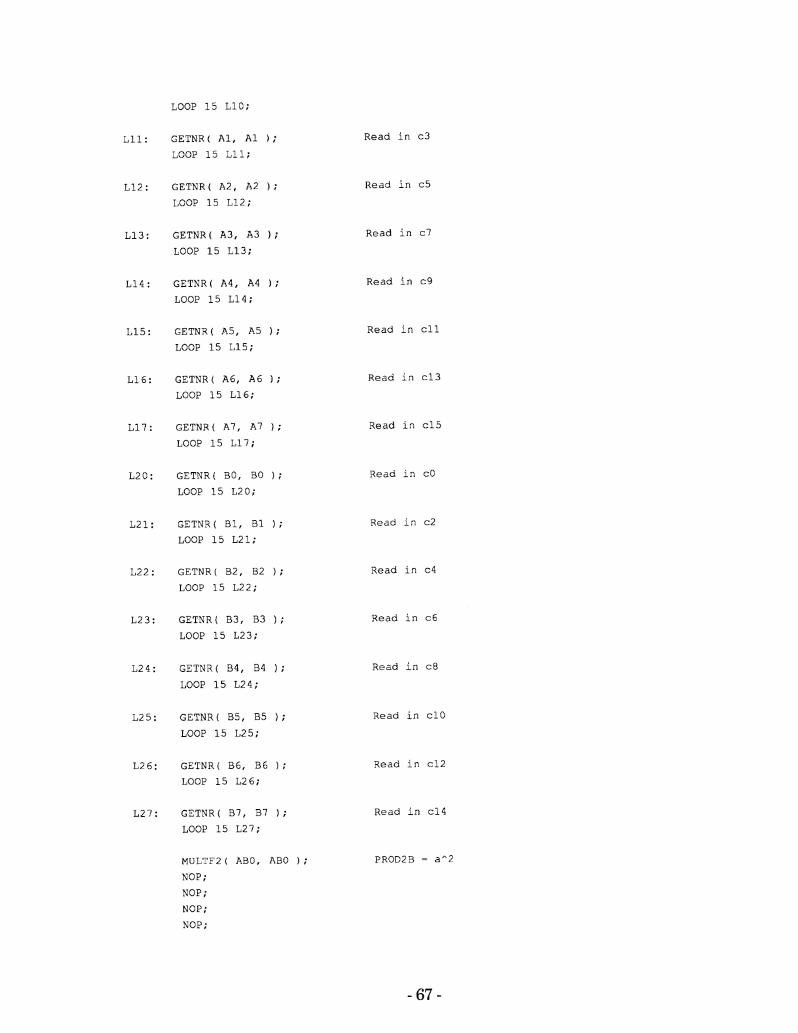
GETNR ( A l , A 1 ) ;
LOOP 15 L 1 1 ;
GETNR ( A 2 , A2 ) ;
LOOP 15 L 1 2 ;
GETNR ( A 3 , A 3 ) ;
LOOP 15 L 1 3 ;
GETNR ( A 4 , A4 ) ;
LOOP 15 L 1 4 ;
GETNR ( A 5 , A 5 ) ;
LOOP 15 L 1 5 ;
G E T N R ( A 6 , A 6 ) ;
LOOP 15 L 1 6 ;
GETNR ( A 7 , A 7 ) ;
LOOP 15 L 1 7 ;
G E T N R ( BO, BO ) ;
LOOP 15 L 2 0 :
G E T N R ( B 1 , B1 1:
LOOP 1 5 L 2 1 ;
G E T N R ( B 2 , B2 ) ;
LOOP 15 L 2 2 ;
G E T N R ( 8 4 , B4 I ; LOOP 15 L 2 4 ;
GETNR ( B5, B5 ) ;
LOOP 15 L 2 5 ;
G E T N R ( B 6 , B 6 ) ;
LOOP 15 L 2 6 ;
GETNR ( B 7 , B7 ) ;
LOOP 15 L 2 7 :
MULTF2 ( ABO, ABO ) ;
NOP ;
NOP ;
NOP ;
NOP;
R e a d in c 3
R e a d in c5
R e a d in c 7
R e a d in c 9
R e a d in c l l
R e a d in c13
R e a d in c 1 5
R e a d in c O
R e a d in c 2
R e a d in c 4
R e a d in c 6
R e a d in c 8
R e a d i n c 1 0
R e a d in c 1 2
R e a d in c 1 4
PROD2B = a - 2
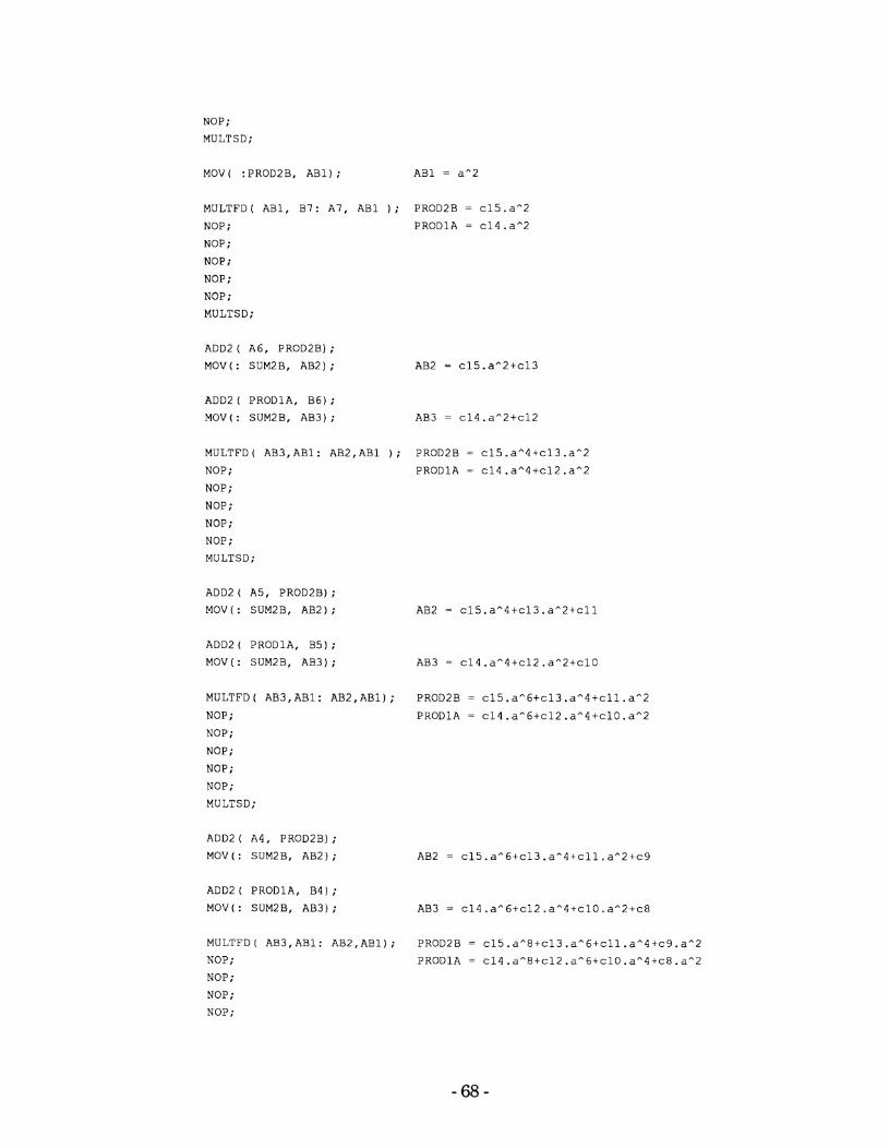
NOP;
MULTSD;
MULTFD ( AB1, B7: A7, AB1 ) ; PROD2B = c15. a"2
NOP; PRODlA = c14. a"2
NOP ;
NOP;
NOP ;
NOP;
MULTSD;
ADD2 ( A6, PROD2B);
MOV ( : SUMZB, AB2) ; AB2 = c15.aA2+c13
MULTFD( AB3,ABl: AB2,ABl ) ; PROD2B = c15.aA4tc13.a^2
NOP; PRODlA = c14.a"4+c12.an2
NOP ;
NOP;
NOP;
NOP ;
MULTSD;
ADD2 ( AS, PROD2B);
MOV ( : SUM2B, AB2) ; AB2 = c15.an4+c13.a"2+cll
ADD2 ( PRODlA, B5);
MOV ( : SUM2B, AB3) ; AB3 = c14.a"4+c12.a"2+~10
MULTFD( AB3,ABl: AB2,ABl); PROD2B = c15.a"6+~13.a"4+cll.a"2
NOP ; PRODlA = c14.a"6+c12.a^4+c10.an2
NOP;
NOP ;
NOP;
NOP;
MULTSD:
ADD2 ( A4, PROD2B) ;
MOV ( : SUM2B, AB2) ; AB2 = c15.a^6+~13.a"4+cll.a^2+~9
ADD2 ( PRODlA, B4) ;
MOV ( : SUM2B, AB3) ; AB3 = c14.a^6+c12.a^4+c10.an2+c8
MULTFD( AB3,ABl: AB2,ABl); PROD2B = c15.a"8tc13.an6+cll.an4+c9.a"2
NOP; PRODlA = c 1 4 . a " 8 t c 1 2 . a n 6 t c 1 0 . a n 4 t c 8 . a ~ 2
NOP ;
NOP ;
NOP;
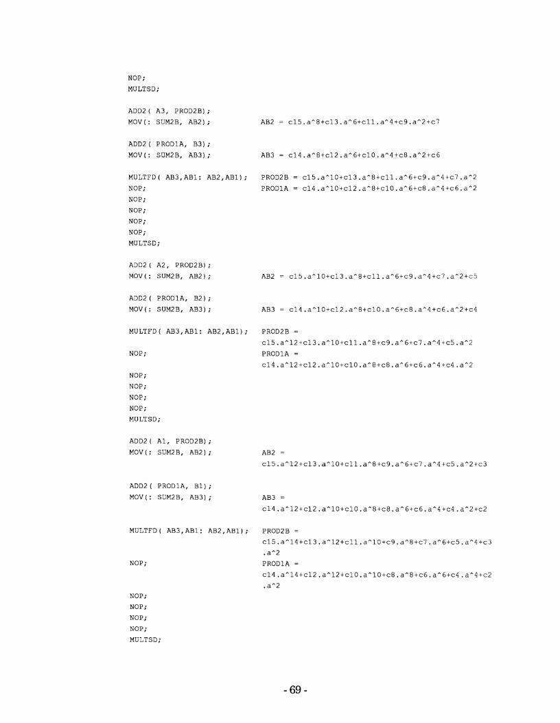
NOP;
MULTSD;
ADD2 ( PRODlA, B3);
MOV ( : SUM2B, AB3) ;
MULTFD( AB3,ABl: AB2,ABl); PROD2B = c l 5 . a " l O + c l 3 . a " 8 + c l l . a " 6 t c 9 . a ~ 2
NOP; PRODlA = ~ 1 4 . a " 1 0 + ~ 1 2 . a " 8 + ~ 1 0 . a " 6 + ~ 8 . a ~ 2
NOP;
NOP ;
NOP;
NOP ;
MULTSD;
ADD2 ( PRODlA, B2);
MOV(: SUMZB, AB3); AB3 = c14.a"10+c12.a"8+c10.a"6+c8.aa4+c6.a~2+c4
MULTFD ( AB3, AB1: AB2,ABl) ; PROD2B =
c15.aA12+c13.aa10+cll.aA8+c9.aA6tc7.aa4+c5.a''2
NOP; PRODlA =
c14.a"12+c12.a"10+c10.a"8+c8.a~6+c6.aA4+c4.a"2
NOP;
NOP;
NOP;
NOP;
MULTSD;
ADD2 ( Al, PROD2B) ;
MOV(: SUM2B, AB2);
ADD2 ( PRODlA, B1) ;
MOV( : SUM2B, AB3) ;
MULTFD ( AB3, AB1: AB2, AB1) ; PROD2B =
c15.a"14+c13.a"12+cll.a"1O+c9.a"8tc7.a"6+c5.a"4+c3
. a"2 NOP; PRODlA =
c14.a"14+c12.a"12tclO.a"1Ot~8.a~8+~6.a~6+~4.a"4+~2
. a"2 NOP;
NOP ;
NOP;
NOP;
MULTSD;
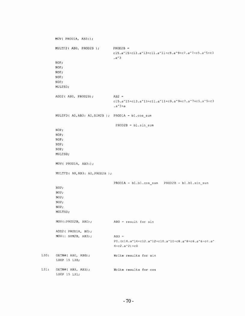
MOV ( P R O D l A , AB3 : ) ;
MULTF2 ( ABO, PROD2B ) ; PROD2B =
c15.a^15+c13.a^13+cll.aA11+c9.a~9+c1.afi7tc5.aA5+c3
. a-3 NOP;
NOP;
NOP ;
NOP ;
NOP;
MULTSD;
ADD2 ( ABO, PROD2B) ;
MULTFD ( AO, A B 3 : AO, SUM2B ) ; P R O D l A = b l . c o s - s u m
NOP;
NOP ;
NOP;
NOP;
NOP ;
MULTSD;
M O V ( P R O D l A , A B 3 : ) ;
MULTFD ( AO, A B 3 : AO, PROD2B ) ;
P R O D l A = b l . b l . c o s - s u m PROD2B = b l . b l . s i n p s u m
NOP ;
NOP ;
NOP ;
NOP ;
NOP;
MULTSD;
MOV ( : PROD2B, ABO) ;
ADD2 ( P R O D l A , BO) ;
MOV(: SUMZB, A B 3 ) ;
L 3 0 : GETNW ( ABO, ABO) ;
LOOP 15 L 3 0 ;
L 3 1 : GETNW ( A B 3 , A B 3 ) ;
LOOP 15 L 3 1 ;
ABO = r e s u l t f o r s i n
Write r e s u l t s f o r s i n
W r i t e r e s u l t s for cos
Appendix D - Software for Trqjectory Planning
Program - p 1 a n . a
A u t h o r - C r a i g S a y e r s
D a t e - Dec 1990
P u r p o s e - T h i s r o u t i n e c a l c u l a t e s t h e f o r w a r d k i n e m a t i c s
f o r a t h r e e - l i n k p l a n a r m a n i p u l a t o r .
The i n p u t i s t h r e e a n g l e s i n t h e r a n g e
-1 <= a <= 1, where a i s some f r a c t i o n o f
P I r a d i a n s .
The r o u t i n e a l s o c a l c u l a t e s t h e c a r t e s i a n d i s t a n c e
be tween t h e e n d - e f f e c t o r a n d a s p e c i f i e d t a r g e t
p o s i t i o n . ( T h i s c a l c u l a t i o n i s i n a c c u r a t e f o r s m a l l
d i s t a n c e s due t o i n a c c u r a c i e s i n t h e s q u a r e r o o t
r o u t i n e - s e e r e p o r t on s q u a r e r o o t r o u t i n e f o r
f u r t h e r d e t a i l s ) .
R e g i s t e r Map f o r c a l c u l a t i n g s i n e a n d c o s i n e
ABO AB1
AB2
AB3
AB4
AB5
AB 6
AB7
I n p u t j o i n t a n g l e s
Temporary S t o r a g e
s i n 3
C O S ~
s i n 2
c o s 2
s i n 1
c o s l
b l c o n s t a n t
c 3 c o n s t a n t
c 5 c o n s t a n t
c 7 c o n s t a n t
c9 c o n s t a n t
c l l c o n s t a n t
c 1 3 c o n s t a n t
c 1 5 c o n s t a n t
CO c o n s t a n t
C2 c o n s t a n t
C4 c o n s t a n t
C6 c o n s t a n t
C 8 c o n s t a n t
C10 c o n s t a n t
C12 c o n s t a n t
C14 c o n s t a n t
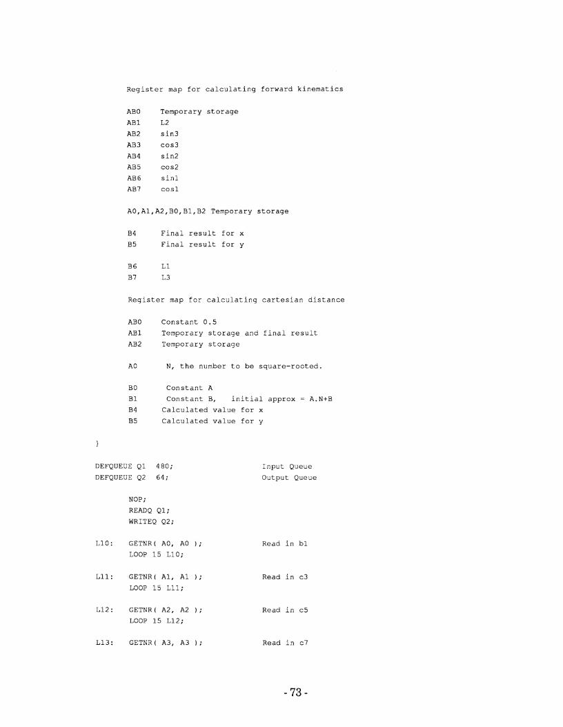
R e g i s t e r m a p f o r c a l c u l a t i n g f o r w a r d k i n e m a t i c s
T e m p o r a r y s torage
L 2
s i n 3
C O S ~
s i n 2
c o s 2
s i n 1
cos l
AO,Al,AZ,BO, B l , B 2 T e m p o r a r y s t o r a g e
B 4 F i n a l r e s u l t f o r x
B5 F i n a l r e s u l t f o r y
R e g i s t e r m a p f o r c a l c u l a t i n g c a r t e s i a n d i s t a n c e
ABO C o n s t a n t 0 . 5
AB1 T e m p o r a r y s t o r a g e a n d f i n a l r e s u l t
AB2 T e m p o r a r y s t o r a g e
A 0 N, t h e n u m b e r t o be s q u a r e - r o o t e d .
B 0 C o n s t a n t A
B 1 C o n s t a n t B, i n i t i a l a p p r o x = A.N+B
B 4 C a l c u l a t e d v a l u e f o r x
85 C a l c u l a t e d v a l u e f o r y
DEFQUEUE Q 1 4 8 0 ;
DEFQUEUE Q2 6 4 ;
NOP ;
READQ Q1;
WRITEQ Q2;
L 1 0 : GETNR( AO, A0 ) ;
LOOP 1 5 L10 ;
L 1 1 : GETNR( A l , A1 ) ;
LOOP 1 5 L11 ;
L 1 2 : GETNR( A2, A2 ) ;
LOOP 1 5 L12 ;
I n p u t Q u e u e
O u t p u t Q u e u e
R e a d i n bl
R e a d i n c 3
R e a d i n c 5
R e a d i n c 7
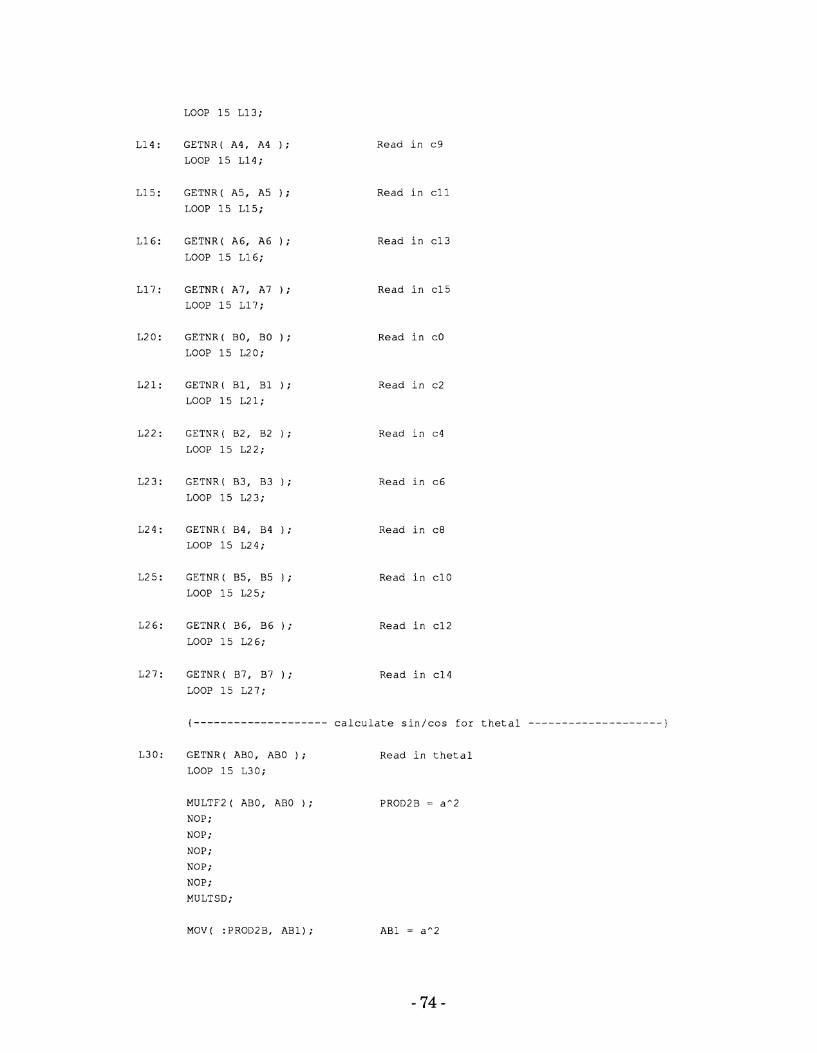
LOOP 15 L13:
GETNR ( A4, A4 ) ;
LOOP 15 L 1 4 ;
R e a d in c 9
GETNR ( A5, A5 ) ;
LOOP 15 L 1 5 ;
R e a d in c l l
GETNR ( A6, A 6 ) ;
LOOP 15 L 1 6 ;
R e a d in c 1 3
GETNR ( A7, A7 ) ;
LOOP 15 L 1 7 ;
R e a d i n c15
GETNR( BO, BO ) ;
LOOP 15 L20:
R e a d in cO
GETNR( B1, B 1 ) ;
LOOP 15 L21:
R e a d in c 2
GETNR ( B2, B2 ) ;
LOOP 1 5 L22:
R e a d i n c 4
GETNR( 83, 83 ) ;
LOOP 15 L23 ;
R e a d in c 6
GETNR( 8 4 , B4 ) ;
LOOP 15 L 2 4 ;
R e a d in c 8
GETNR( B5 , B 5 1 ;
LOOP 15 L 2 5 ;
R e a d i n c 1 O
GETNR( B6, B 6 ) ;
LOOP 15 L 2 6 ;
R e a d in c 1 2
GETNR ( B7, B7 ) ;
LOOP 15 L 2 7 ;
R e a d in c 1 4
GETNR ( ABO, ABO ) ; R e a d in t h e t a 1
LOOP 15 L 3 0 ;
MULTF2 ( ABO, ABO ) ; PROD2B = a A 2
NOP ;
NOP;
NOP;
NOP ;
NOP;
MULTSD;
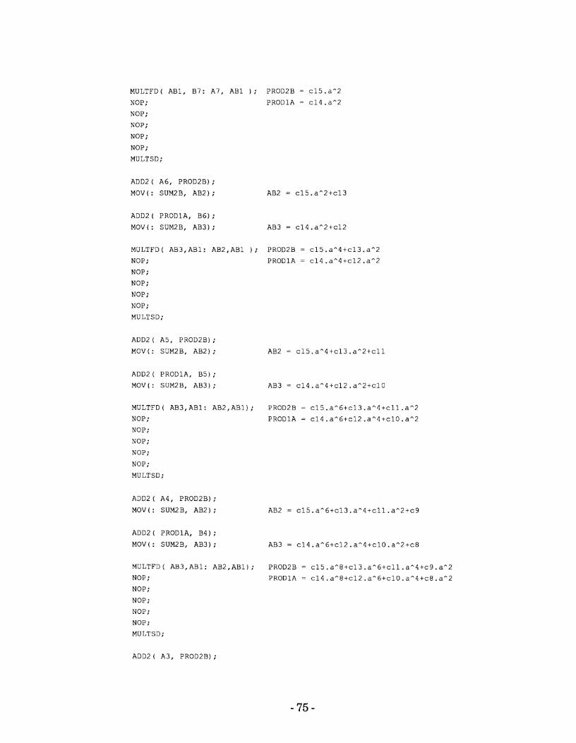
MULTFD( AB1, B7: A7, AB1 ) ; PROD2B = c15.aA2
NOP; PRODlA = c14 .aA2
NOP;
NOP;
NOP ;
NOP;
MULTSD;
ADD2 ( A6, PROD2B);
MOV ( : SUM2B, AB2) ; AB2 = c15.aA2tc13
ADD2 ( PRODlA, B6) ;
MOV(: SUM2B, AB3); AB3 = c14.aA2+c12
MULTFD( AB3,ABl: AB2,ABl ) ; PROD2B = c15.aA4+c13.a^2
NOP ; PRODlA = c14.aA4tc12.aA2
NOP;
NOP;
NOP;
NOP;
MULTSD;
ADD2 ( A5, PROD2B) ;
MOV ( : SUM2B, AB2) ; AB2 = c15.aA4+c13.a^2+cll
ADD2 ( PRODlA, B5);
MOV ( : SUM2B, AB3) ; AB3 = c14.aA4+c12.aA2+c10
MULTFD( AB3,ABl: AB2,ABl); PROD2B = c15.a^6+c13.aA4+cll.aA2
NOP ; PRODlA = c14.aA6+c12.aA4tc10.aA2
NOP;
NOP ;
NOP;
NOP;
MULTSD;
ADD2 ( A4, PROD2B) ;
MOV ( : SUM2B, AB2) ;
ADD2 ( PRODlA, B4) ;
MOV(: SUMZB, AB3); AB3 = c14.aA6+c12.aA4+c10.a^2+c8
MULTFD( AB3,ABl: AB2,ABl); PROD2B = c15.aA8+c13.aA6+cll.aA4tc9.a^2
NOP ; PRODlA = c14 .aA8+c12 .aA6+c10 .aA4tc8 .aA2
NOP;
NOP;
NOP;
NOP ;
MULTSD;
ADD2 ( PRODlA, B3) ;
MOV(: SUMZB, AB3) ;
MULTFD( AB3,ABl: AB2,ABl); PROD2B = ~15.a*10+~13.a*8+cll.a*6+~9.a*4+~7.a*2
NOP; PRODlA = c14.a*10+~12.a*8+~10.a*6+~8.a*4+~6.a*2
NOP;
NOP;
NOP;
NOP;
MULTSD:
ADD2 ( PRODlA, B2) ;
MOV(: SUMZB, AB3); AB3 = c 1 4 . a * 1 0 + c 1 2 . a A 8 t c 1 0 . a * 6 + c 8 . a ^ 2 + c 4
MULTFD ( AB3, AB1: AB2, AB1) ; PRODZB =
c15.a*12+c13.a*10+cll.a*8+~9.a^4+~5.a*2
NOP; PRODlA =
c14.a*12+c12.a*10+clO,a~8+c8.a*6tc6.a~4+c4.aA2
NOP;
NOP;
NOP;
NOP ;
MULTSD;
ADD2 ( Al, PRODZB) ;
MOV ( : SUMZB, AB2) ;
ADD2 ( PRODlA, B1) ;
MOV(: SUM2B, AB3); AB3 =
c14,a*12tc12.aA10tclO.a*8tc8.a^6+c6.a*4+c4.aA2tc2
MULTFD ( AB3, AB1: AB2,ABl) ; PROD2B =
c15.a*14+c13.a~12+cll.a^10+c9.a^8+c7.aA6+c5.a*4+c3
. a*2 NOP ; PRODlA =
c 1 4 . a A 1 4 + c 1 2 . a ^ 1 2 + c 1 0 . a A 1 0 + c 6 . a ^ 6 + c 4 . a * 4 + c 2
. aA2 NOP;
NOP;
NOP;
NOP ;
MULTSD;
MOV( PRODlA, AB3 : ) ;
MULTF2 ( ABO, PROD2B ;
NOP ;
NOP;
NOP ;
NOP ;
NOP;
MULTSD;
ADD2 ( ABO, PROD2B) ;
PRODZB =
c15.a*15+c13.a*13tcll.a~11tc9.a*9+~7.a*7+~5.a*5tc3
. a-3
ABZ =
c15.aA15+c13.aA13+cll.a~11+c9.a*9+c1.aA7+c5.a*5+c3
. a A 3 + a
MULTFD ( AO, AB3 : AO, SUM2B ) ; PRODlA = b l . c o s - s u m
PROD2B = b l . s i n _ s u m
NOP ;
NOP;
NOP;
NOP;
NOP;
MULTSD;
MOV ( PRODlA, AB3 : ) ;
MULTFD( AO,AB3: AO,PROD2B); PRODlA = b l . b l . c o s - s u m PROD2B = b l . b l . s i n - s u m
NOP;
NOP ;
NOP ;
NOP;
NOP;
MULTSD;
MOV ( : PRODZB, ABGI ; AB6 = r e s u l t f o r s i n ( t h e t a l )
SUM2B =
P I . ( c 1 4 . a ^ 1 4 + c 1 2 . a A 1 2 + c 1 0 . a n 1 0 t c 8 . a ~ 6 + c 4 . a A
4 t c 2 . a A 2 ) tc0
MOV(: SUM2B, AB7) ; AB7 = r e s u l t f o r c o s ( t h e t a l )
{-------------------- c a l c u l a t e s i n / c o s f o r t h e t a 2 ....................
L 3 1 : GETNR ( ABO, ABO ) ; R e a d i n t h e t a 2
LOOP 15 L 3 1 ;
MULTF2 ( ABO, ABO ) ; PROD2B = a n 2
NOP;
NOP;
NOP;
NOP;
NOP;
MULTFD t AB1, B7 : Al, AB1 ) ; PROD2B = c15. a^2
NOP; PRODlA = c14.aA2
NOP;
NOP;
NOP;
NOP;
MULTSD;
ADD2 ( PRODlA, B6);
MOV(: SUM2B. AB3); AB3 = c14.aA2+c12
MULTFD( AB3, AB1: AB2, AB1 );PROD2B = c15.a^4+c13.aA2
NOP ; PRODlA = c14.a^4+c12.aA2
NOP;
NOP;
NOP;
NOP;
MULTSD;
ADD2 ( PRODlA, B5);
MOV(: SUMZB, AB3);
MULTFD( AB3,ABl: AB2,ABl); PROD2B = c15.a^6+~13.a^4+cll.a^2
NOP; PRODlA = c14.aA6+c12.a"4+c10.a"2
NOP;
NOP ;
NOP;
NOP;
MULTSD;
ADD2 ( PRODlA, B4) ;
MOV(: SUMZB, AB3); AB3 = ~14.a^6+~12.a^4+clO.a^2+~8
MULTFD( AB3,ABl: AB2,ABl); PROD2B = c15.aA8+c13.a^6+cll.a^4+c9.aa2
NOP; PRODlA = c14 .aA8+c12 .a^6+c10 .a^4 tc8 .aa2
NOP;
NOP;
NOP;
NOP;
ADD2 ( P R O D l A , B 3 ) ;
MOV ( : SUMZB, A B 3 ) ;
MULTFD( A B 3 , A B l : A B 2 , A B l ) ; PROD2B = c15.an10+c13.a*8+cll.an6+c9.aA4+c7.a*2
NOP; P R O D l A = c14.aA10+c12.aA8+c10.an6+c8.a*4+c6.aA2
NOP ;
NOP;
NOP;
NOP;
MULTSD;
ADD2 ( P R O D l A , B 2 ) ;
MOV( : SUM2B, A B 3 ) ;
MULTFD ( AB3, A B 1 : A B 2 , A B l ) ; PROD2B =
c15.aA12+c13.aA10+cll.an8+c9.a*6tc7.aa4+c5.a*2
NOP; P R O D l A =
c 1 4 . a * 1 2 + c 1 2 . a A 1 0 t c 1 0 . a * 8 + c 8 . a ^ 4 + c 4 . a A 2
NOP;
NOP ;
NOP ;
NOP ;
MULTSD;
ADD2 ( A l , PROD2B) ;
MOV(: SUMZB, A B 2 ) ; AB2 =
c15.aA12+c13.a*10+cll.a*8+c9.an6+c7.a^4+c5.aA2+c3
ADD2 ( P R O D l A , B 1 ) ;
M O V ( : SUM2B, A B 3 ) ; AB3 =
c14.a*12+c12.a"10+clO.a*8+c8.an6+c6.a^4+c4.a*2+c2
MULTFD ( AB3, A B 1 : AB2, A B 1 ) ; PROD2B =
c15.aA14tc13.a*12tcll.a*10+c9.aA8+c7.aA6+c5.a*4+c3
. aA2
P R O D l A =
c 1 4 . a * 1 4 + c 1 2 . a A 1 2 t c l O . a A 1 O t c 8 . a ~ 6 t c 4 . a A 4 t c 2
. a"2
NOP;
NOP ;
NOP;
NOP;
NOP;
MULTSD;
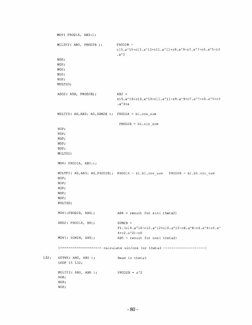
MOV ( P R O D l A , AB3 : ;
MULTF2 ( ABO, PROD2B ) ;
NOP ;
NOP;
NOP ;
NOP;
NOP;
MULTSD;
ADD2 ( ABO, P R O D Z B ) ; AB2 =
c15.aA15tc13.aA13+cll.aA11+c9.aA9+c7.aA7+c5.aA5+c3
. a A 3 + a
MULTFD ( AO, A B 3 : AO, SUM2B ) ; P R O D l A = b l . c o s - s u m
PRODZB = b l . s i n - s u m
NOP;
NOP ;
NOP ;
NOP ;
NOP ;
MULTSD:
MOV ( P R O D l A , AB3 : ) ;
MULTFD( A O , A B 3 : A 0 , P R O D Z B ) ; P R O D l A = b l . b l . c o s - s u m PROD2B = b l . b l . s i n _ s u m
NOP;
NOP;
NOP;
NOP;
NOP;
MULTSD;
MOV(:PRODZB, A B 4 ) ; AB4 = r e s u l t f o r s i n ( t h e t a 2 )
ADD2 ( P R O D l A , BO) ;
MOV ( : SUMZB, A B 5 ) ;
SUM2B =
PI.(c14.aA14+c12.aA12+c10.aA1Otc8.aA8+c6.aA6+c4.aA
4 + c 2 . a A 2 ) + c 0
AB5 = r e s u l t f o r c o s ( t h e t a 2 )
(-------------------- c a l c u l a t e s i n / c o s f o r t h e t a 3 - - - - - - - - - - - - - - - - - - - - )
L 3 2 : GETNR ( ABO, ABO ) ; R e a d i n t h e t a 3
LOOP 15 L 3 2 ;
MULTFZ ( ABO, ABO ) ;
NOP;
NOP;
NOP:
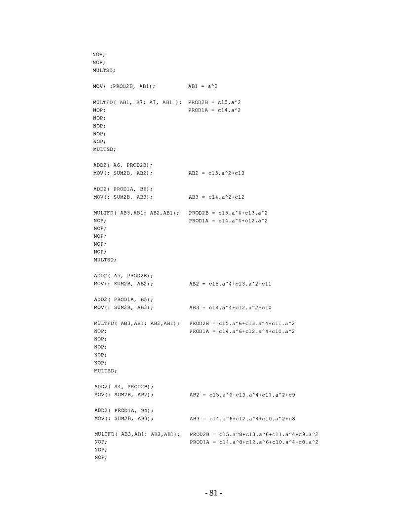
NOP ;
NOP;
MULTSD;
MULTFD ( AB1, B7: A7, AB1 ) ; PROD2B = c15. a"2
NOP; PRODlA = c14.aA2
NOP ;
NOP ;
NOP;
NOP ;
MULTSD;
MULTFD ( AB3,ABl: AB2,ABl) ; PROD2B = c15.an4+c13.a"2
NOP; PRODlA = c14.an4+c12.a"2
NOP;
NOP;
NOP ;
NOP ;
MULTSD;
ADD2 ( PRODlA, B5) ;
MOV ( : SUM2B, AB3) ; AB3 = c14.a"4+c12.a"2+~10
MULTFD( AB3,ABl: AB2,ABl); PROD2B = cl5.a"6+~13.a"4+cll.a"2
NOP; PRODlA = c14. aA6+c12. aA4 tc10. a"2
NOP;
NOP;
NOP;
NOP;
MULTSD:
ADD2 ( PRODlA, B4) ;
MOV( : SUM2B, AB3) ; AB3 = c14.an6+c12.a"4tc10.a^2sc8
MULTFD( AB3,ABl: AB2,ABl); PROD2B = c15.a"8+c13.a"6+cll.aA4+c9.a"2
NOP; PRODlA = c14.an8+c12.a"6+c10.a"4+c8.an2
NOP;
NOP ;

NOP ;
NOP ;
MULTSD;
ADD2 ( A3, PROD2B) ;
MOV ( : SUM2B, AB2 ) ; AB2 = c15.aA8+c13.aA6+cl l .aA4+c9.a"2+c7
MULTFD( AB3,ABl: AB2,ABl); PROD2B = c 1 5 . a * 1 0 + c 1 3 . a A 8 + c l l . a A 6 + c 9 . a ~ 2
NOP ; PRODlA = c 1 4 . a A 1 0 + c 1 2 . a A 8 + c 1 0 . a * 6 + c 6 . a ^ 2
NOP;
NOP;
NOP;
NOP ;
MULTSD;
MULTFD ( AB3, ABI: AB2,ABl) ; PROD2B =
c15.a*12+c13.a*10+cll.a*8+c9.aA6+c7.aA4+cS.aA2
NOP; PRODlA =
c 1 4 . a A 1 2 + c 1 2 . a A 1 0 + c 1 0 . a A 8 + c 8 . a ^ 4 + c 4 . a * 2
NOP;
NOP;
NOP;
NOP;
MULTSD;
ADD2 ( Al, PROD2B) ;
MOV( : SUM2B, AB2) ; AB2 =
c15.aA12+c13.aA10+cll.a*8+c9.a*6+c7.a*4+c5.aA2+c3
MULTFD ( AB3, AB1: AB2, AB1) ; PROD2B =
c 1 5 . a A 1 4 + c 1 3 . a A 1 2 t c l l . a * 1 0 + c 9 . a A 8 t c 7 . a A 6 + c 5 . a A 4 + c 3
. aA2 PRODlA =
c14.a*14+c12.a*12+clO.a*10+c8.aA8+c6.a*6+c4.a~4+c2
. a*2
NOP:
NOP;
NOP;
NOP;
NOP;
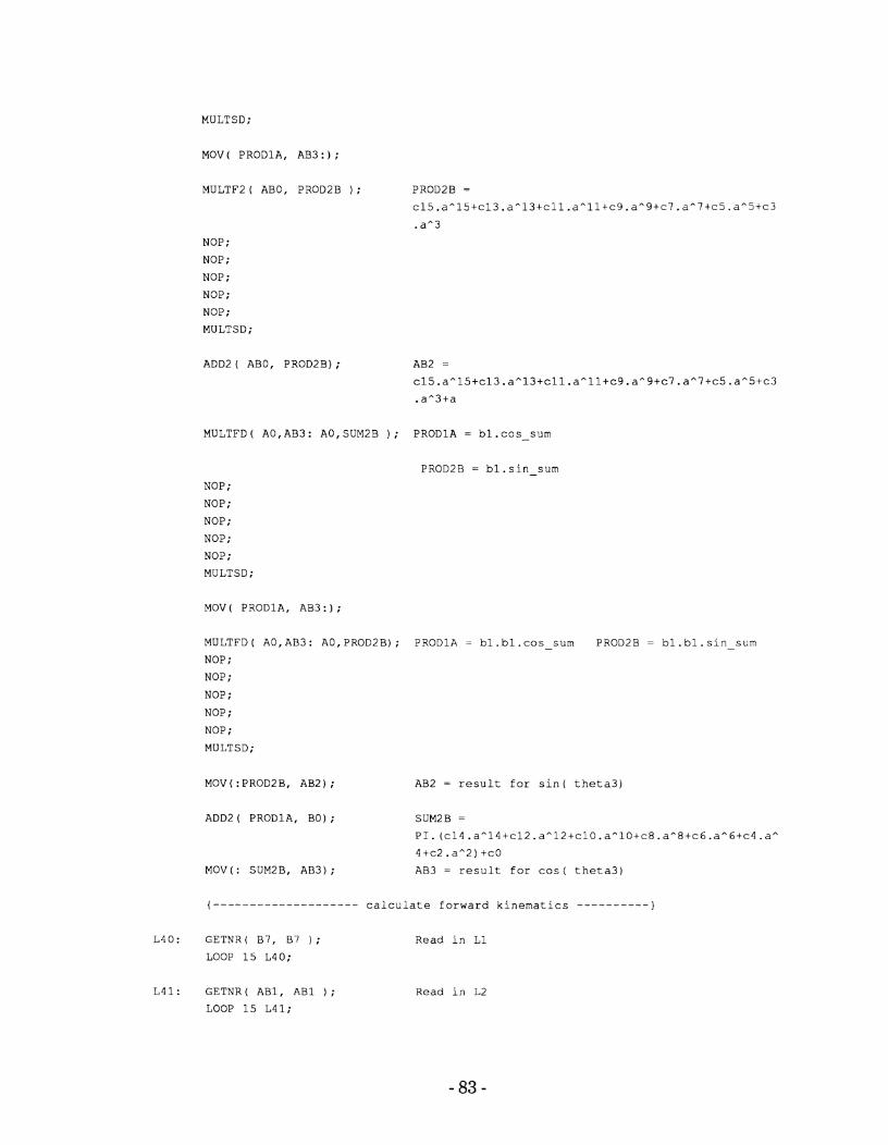
MULTSD;
MOV( P R O D l A , A B 3 : ) ;
MULTF2 ( ABO, PROD2B ) ;
NOP;
NOP;
NOP;
NOP;
NO?;
MULTSD;
ADD2 ( ABO, PROD2B) ;
MULTFD( A O , A B 3 : AO,SUM2B ) ; P R O D l A = b l . c o s - s u m
NOP;
NOP;
NOP;
NO? ;
NOP;
MULTSD:
MOV ( P R O D l A , AB3 : ) ;
MULTFD( AO,AB3: A O , P R O D 2 B ) ; PRODlA = b l . b l . c o s - s u m PROD2B = b l . b l . s i n - s u m
NOP ;
NOP;
NOP;
NOP;
NOP;
MULTSD;
MOV ( : PRODZB, A B 2 ) ; AB2 = r e s u l t f o r s i n ( t h e t a 3 )
ADD2 ( PRODlA, B O ) ; SUM2B =
P I . ( c 1 4 . a A 1 4 + c 1 2 . a A 1 2 + c 1 0 . a A 1 0 + c 6 . a ~ 6 + c 4 . a A
4 + c 2 . a A 2 ) + c 0
MOV ( : SUM2B, A B 3 ) ; AB3 = r e s u l t f o r c o s ( t h e t a 3 )
L 4 0 : GETNR( B 7 , B7 ) ;
LOOP 15 L 4 0 :
Read i n L 1
L 4 1 : G E T N R ( AB1, A B 1 ) ; R e a d i n L 2
LOOP 1 5 L 4 1 ;
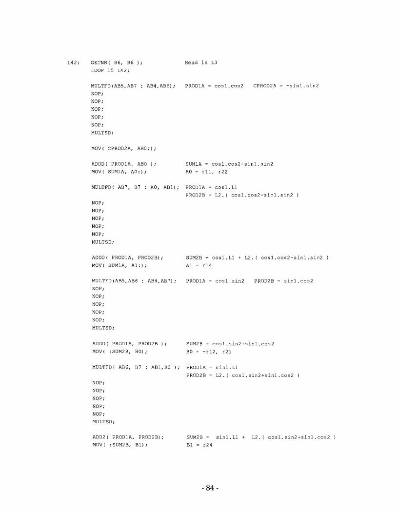
L42: GETNR( B6, B6 ) ;
LOOP 15 L42;
MULTFD(AB5,AB7 : AB4,AB6); PRODlA = cosl.cos2 CPROD2A = -sinl,sin2
NOP;
NOP;
NOP ;
NOP ;
NOP;
MULTSD;
MOV ( CPROD2A. ABO: ) ;
ADDD ( PRODlA, ABO ) ; S U M ~ A = cosl.cos2-sinl.sin2
MOV( SUMlA, AO:) ; A0 = rll, r22
MULTFD ( AB7, B7 : AO, AB1) ; PRODlA = cosl .L1
PROD2B = L2.( cosl.cos2-sinl.sin2 )
NOP ;
NOP ;
NOP;
NOP;
NOP ;
MULTSD;
ADDD ( PRODlA, PROD2B) ; SUM2B = cosl.Ll t L2.( cosl.cos2-sinl.sin2 )
MOV ( SUMlA, Al: ) ; A1 = r14
MULTFD(AB5,ABG : AB4,AB7); PRODlA = cosl.sin2 PROD2B = sinl.cos2
NOP;
NOP;
NOP;
NOP ;
NOP;
MULTSD;
ADDD( PRODlA, PROD2B ; SUM2B = cosl.sin2+sinl.cos2
MOV( :SUM2B, BO); BO = -r12, r21
MULTFD ( AB6, B7 : AB1,BO ) ; PRODlA = sin1 .L1
PROD2B = L2.( cosl.sin2tsinl.cos2 )
NOP;
NOP;
NOP;
NOP;
NOP ;
MULTSD;
ADD2 ( PRODlA, PROD2B) ;
MOV( :SUM2B, B1);
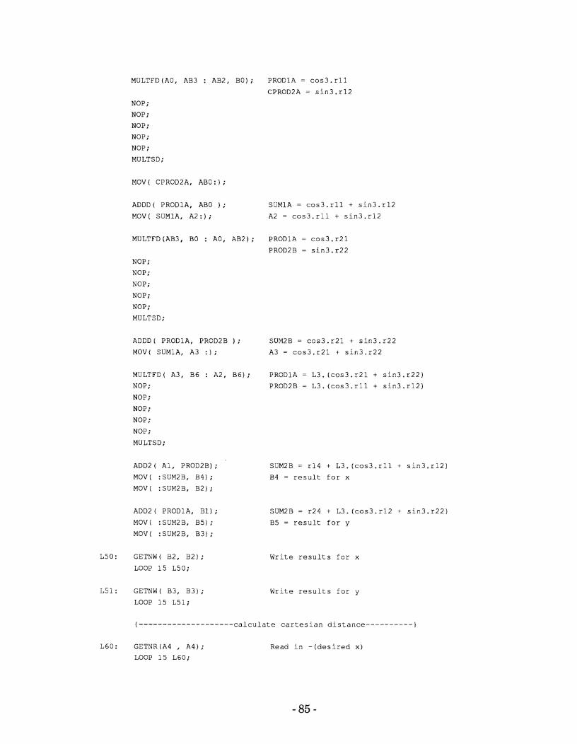
MULTFD(A0, AB3 : AB2, BO); PRODlA = cos3.rll
CPROD2A = sin3.rl2
NOP ;
NOP;
NOP ;
NOP;
NOP;
MULTSD;
MOV ( CPROD2A, ABO : ) ;
ADDD( PRODlA, ABO ) ; SUMlA = cos3.rll + sin3.rl2 MOV( SUMlA, A2:); A2 = cos3.rll + sin3.rl2
MULTFD (AB3, BO : AO, AB2) ; PRODlA = cos3. r21
PROD2B = sin3.r22
NOP;
NOP ;
NOP ;
NOP;
NOP;
MULTSD;
ADDD [ PRODlA, PROD2B ) ; SUM2B = cos3.r-21 + sin3.r22 MOV( SUMlA, A3 : ; A3 = cos3.r21 + sin3.r22
MULTFD( A3, B6 : A2, B6); PRODlA = L3. (cos3.r21 + sin3.r22) NOP; PROD2B = L3.(cos3.rll + sin3.rl2) NOP;
NOP;
NOP;
NOP ;
MULTSD;
ADD2 ( Al, PROD2B) ; SUM2B = r14 t L3.(cos3.rll t sin3.rl2)
MOV( :SUM2B, B4); B4 = result for x
MOV[ :SUM2B, B2);
ADD2 ( PRODlA, Bl); SUM2B = r24 + L3.(cos3.r12 + sin3.r22) MOV( :SUM2B, B5) ; 85 = result for y
MOV( :SUM2B, B3) ;
L51: GETNW( B3, B3);
LOOP 15 L51;
Write results for x
Write results for y
L60: GETNR(A4 , A4); LOOP 15 L60;
Read in -(desired x)
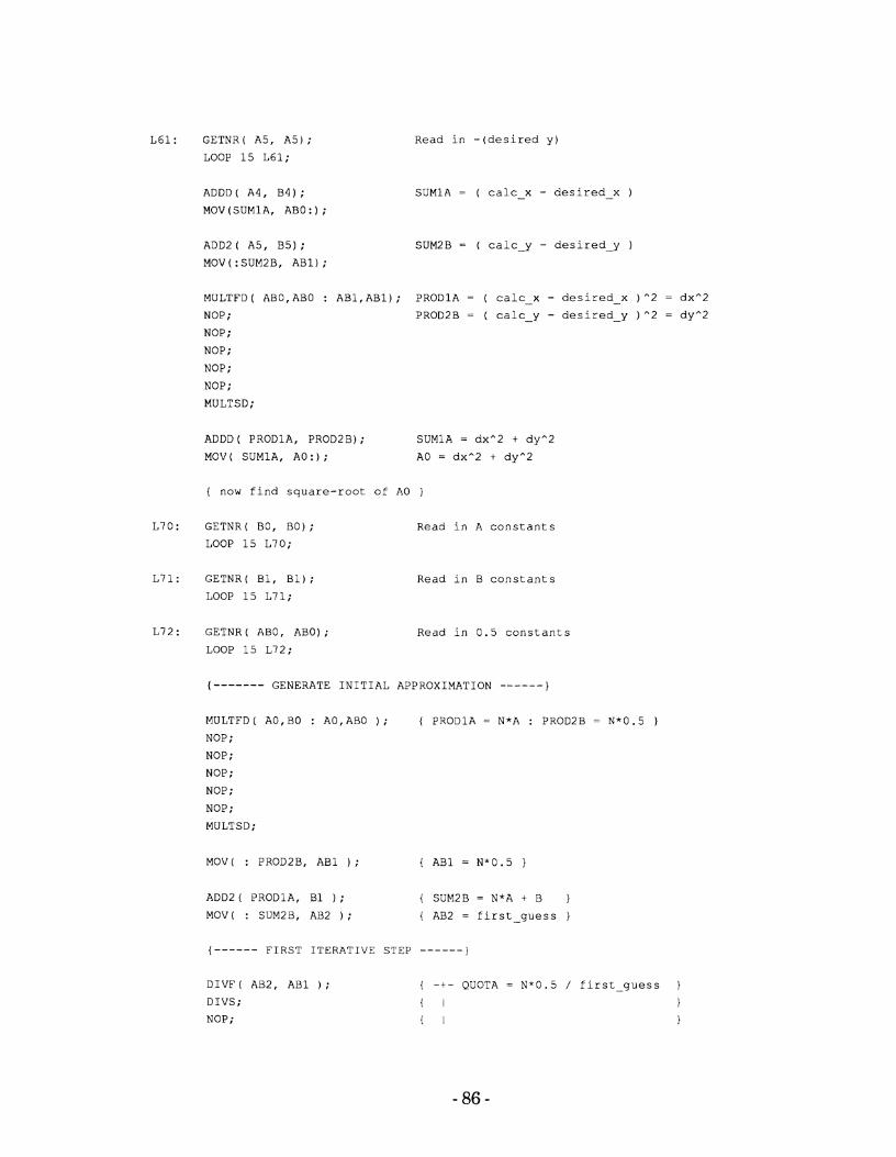
L61: GETNR( A5, A5);
LOOP 15 L61:
ADDD( A4, B4);
MOV (SUMlA, ABO : ) ;
Read in -(desired y)
SUMlA = ( calc-x - desired-x )
ADD2( A5, B5); SUM2B = ( calc-y - desired-y )
MOV ( : SUM2B, AB1) ;
MULTFD( AB0,ABO : AB1,ABl); PRODlA = ( calc-x - desired-x )*2 = dxA2
NOP; PROD2B = ( calc-y - desired - y )^2 = dyA2
NOP;
NOP;
NOP;
NOP ;
MULTSD;
ADDD ( PRODlA, PROD2B) ; SUMlA = dxA2 + dyn2 MOV ( SUMlA, AO: ) ; A0 = dxA2 + dyn2
( now find square-root of A0 )
L70: GETNR( BO, BO) ;
LOOP 15 L70;
L71: GETNR( B1, B1);
LOOP 15 L71;
L72: GETNR( ABO, ABO) ;
LOOP 15 L72;
Read in A constants
Read in B constants
Read in 0.5 constants
(------- GENERATE INITIAL APPROXIMATION ------)
MULTFD ( AO, BO : A0,ABO ) ; { PRODlA = N*A : PROD2B = N*0.5 )
NOP;
NOP;
NOP ;
NOP ;
NOP ;
MULTSD;
ADD2 ( PRODlA, B1 ) ; { SUM2B = N*A t B )
MOV( : SUM2B, AB2 ) ; { AB2 = first-guess )
{ - - - - - - FIRST ITERATIVE STEP - - - - - - )
DIVF ( AB2, AB1 ) ; ( -+- QUOTA = N*0.5 / first-guess
DIVS; ( I )
NOP; I 1
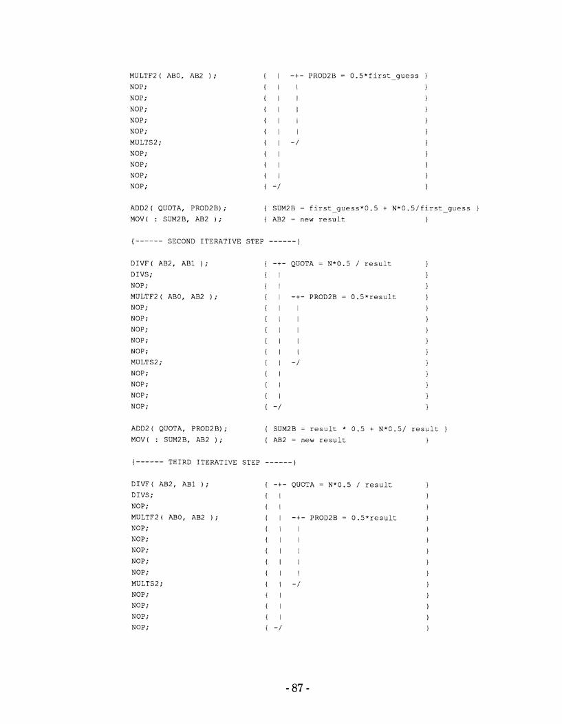
MULTF2 (
NOP;
NOP;
NOP;
NOP;
NOP;
MULTS2;
NOP;
NOP;
NOP;
NOP ;
ABO, AB2 ) ; ( 1 -+-
( I I
( 1 I
i I ( I I
{ I I i 1 - /
( I
( I
( I
( - /
ADD2 ( QUOTA, PROD2B) ; { SUM2B = f i r s t p u e s s * 0 . 5 + N * O . S / f i r s t - g u e s s )
MOV( : SUM2B, AB2 ) ; ( AB2 = n e w r e s u l t )
(------ SECOND I T E R A T I V E S T E P ------)
D I V E ( AB2, A B 1 ) ;
D I V S ;
NOP;
MULTF2 ( ABO, AB2 ) ;
NOP;
NOP ;
NOP;
NOP ;
NOP ;
MULTS2;
NOP;
NOP;
NOP ;
NOP;
( -+- QUOTA = N * 0 . 5 / r e su l t
i I
( I
{ I -+- PROD2B = 0 . 5 * r e s u l t
( I I
{ I I
{ I I
I I
( 1 I ( I -1
i I
i I
1 I
i -/
ADD2 ( QUOTA, PROD2B) ; { SUM2B = r e s u l t * 0 . 5 + N * 0 . 5 / r e s u l t )
MOV ( : SUM2B, AB2 ) ; ( AB2 = n e w r e s u l t 1
{ - - - - - - T H I R D I T E R A T I V E S T E P - - - - - - I
D I V E ( AB2, A B 1 ) ;
D I V S ;
NOP ;
MULTE2 ( ABO, AB2 ) ;
NOP;
NOP ;
NOP;
NOP ;
NOP;
MULTS2 ;
NOP ;
NOP;
NOP;
NOP;
( -+- QUOTA = N * 0 . 5 / r e s u l t
( I
( 1 { I -+- PROD2B = 0 . 5 * r e s u l t
I I i 1
( I I
( : I I
( I I
( I - /
i I
i I
I
{ - /
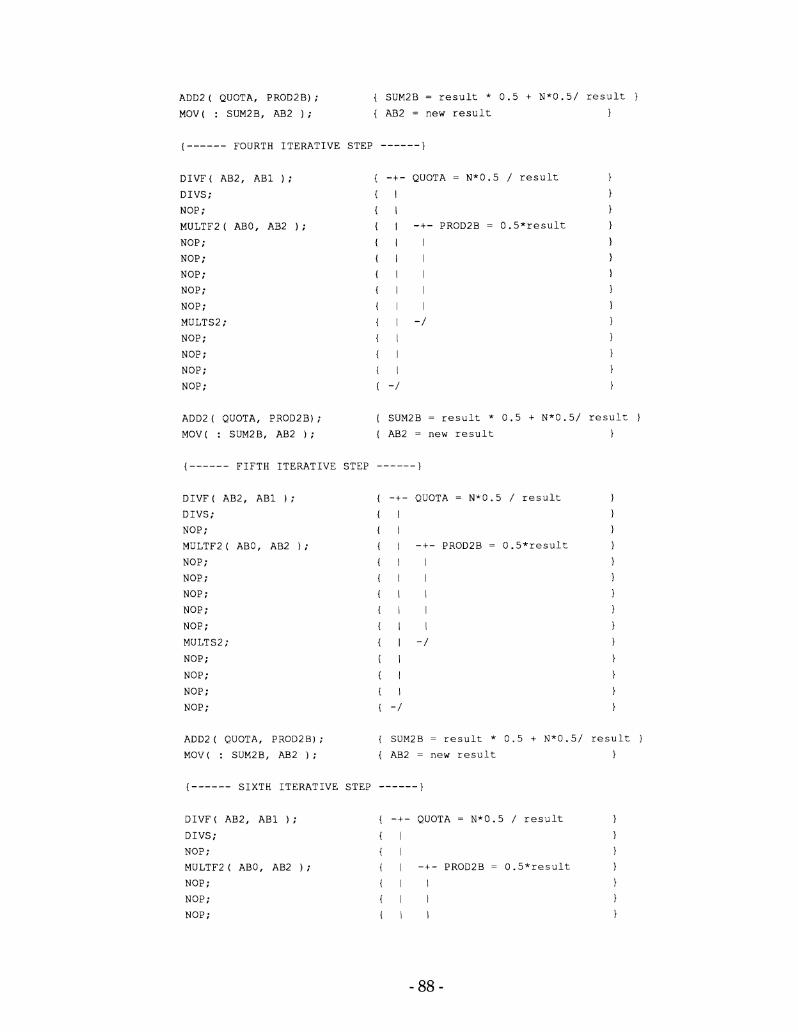
ADD2 ( QUOTA, PRODZB) ; { SUM2B = r e s u l t * 0 . 5 + N * 0 . 5 / r e s u l t 1
MOV ( : SUM2B, AB2 ) ; { AB2 = n e w r e s u l t
( - - - - - - FOURTH ITERATIVE STEP ------)
D I V F ( AB2, AB1 ) ;
DIVS;
NOP ;
MULTF2 ( ABO, AB2 ) ;
NOP;
NOP;
NOP;
NOP;
NOP;
MULTS2 ;
NOP;
NOP ;
NOP;
NOP ;
{ -+- QUOTA = N * 0 . 5 / r e s u l t
i I
t I { I -+- PROD2B = 0 . 5 * r e s u l t
( 1 I I I { I I ( I I
I I
I I - / I I I
I
{ -1
ADD2 ( QUOTA, PROD2B) ; ( SUM2B = r e s u l t * 0 . 5 + N * 0 . 5 / r e s u l t )
MOV( : SUM2B, AB2 ) ; ( AB2 = n e w r e s u l t 1
{------ F I F T H ITERATIVE STEP ------)
DIVF ( AB2, AB1 ) ;
DIVS;
NOP ;
MULTF2 ( ABO, AB2 ) ;
NOP;
NOP ;
NOP;
NOP;
NOP;
MULTSZ;
NOP;
NOP ;
NOP ;
NOP ;
QUOTA = N*0.5 / r e s u l t
)
)
-+- PROD2B = 0 . 5 * r e s u l t 1
I )
I 1 I 1 I )
I I - / 1
ADD2 ( QUOTA, PRODZB) ; { SUM2B = r e s u l t * 0 . 5 + N * 0 . 5 / r e s u l t )
MOV ( : SUMZB, AB2 ) ; { AB2 = n e w r e s u l t 1
{ - - - - - - SIXTH ITERATIVE STEP - - - - - - )
D I V F ( AB2, AB1 ) ; { -+- QUOTA = N*0.5 / r e s u l t )
DIVS; { I 1 NOP; { I )
MULTF2 ( ABO, AB2 ) ; { I -+- PROD2B = 0 . 5 * r e s u l t 1 NOP ; { I I )
NOP; I 1 )
NOP; { I I )
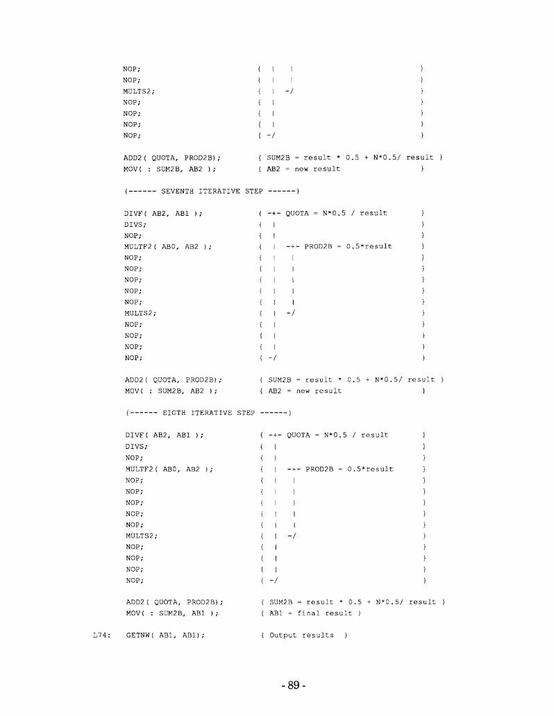
NOP;
NOP;
MULTS2;
NOP;
NOP ;
NOP;
NOP;
ADD2 ( QUOTA, PROD2B) ; { SUM2B = r e s u l t * 0 . 5 + N * 0 . 5 / r e s u l t }
MOV( : SUM2B, AB2 ) ; { AB2 = n e w r e s u l t }
{ - - - - - - SEVENTH I T E R A T I V E S T E P - - - - - - )
D I V F ( AB2, A B 1 ) ;
D I V S ;
NOP ;
MULTF2 ( ABO, AB2 ) ;
NOP;
NOP;
NOP;
NOP;
NOP;
MULTS2;
NOP;
NOP ;
NOP;
NOP ;
QUOTA = N * 0 . 5 / r e s u l t
ADD2 ( QUOTA, PRODZB) ; { SUM2B = r e s u l t * 0 . 5 + N * 0 . 5 / r e s u l t }
MOV ( : SUMZB, AB2 ) ; { AB2 - n e w r e s u l t 1
{ - - - - - - E I G T H I T E R A T I V E S T E P ------)
D I V F ( AB2, A B 1 1;
D I V S ;
NOP;
MULTF2 ( ABO, AB2 ) ;
NOP ;
NOP;
NOP;
NOP;
NOP ;
MULTS2 ;
NOP;
NOP ;
NOP;
NOP;
{ -+- QUOTA = N * 0 . 5 / r e s u l t
I
I { I -+- PROD2B = 0 . 5 * r e s u l t
{ I I I I
I I
{ I I
{ I I
i I - / i I
i I
1
{ - /
ADD2 ( QUOTA, PROD2B) ; { SUM2B = r e s u l t * 0 . 5 t N * 0 . 5 / r e s u l t )
MOV( : SUM2B, AB1 1; { A B 1 = f i n a l r e s u l t )
L 7 4 : GETNW( AB1, A B 1 ) ; { O u t p u t r e s u l t s )

LOOP 15 L74;
STOP; END;