the ho and lee interest rate model - thunderbird...
TRANSCRIPT

Analytical Implementation of the Ho and Lee Model for the Short Interest Rate
Dwight Grant†,* and Gautam Vora**
March 1999 Revised: November 11, 2001
JEL classification: C15, C63, G12, G13 Keywords: Term-Structure Model; Ho-Lee Model; Interest Rate Evolution; Short Rate Model;
No-Arbitrage Model
HL_GFJ_Rev_EndNotes © 1999-2001

Analytical Implementation of the Ho and Lee Model for the Short Interest Rate
Abstract
Ho and Lee introduced the first no-arbitrage model of the evolution of the short interest rate. When expositing the Ho and Lee model, other authors used the method of numerical solutions and forward induction, an approach pioneered by Black, Derman and Toy for their own model much later. This standard method of implementation is relatively complex and time-consuming when applied to scenarios that enable the use of an interest rate lattice. Under many assumptions, however, the Ho and Lee model will generate an interest rate tree. Under these circumstances, implementation via numerical methods and forward induction appear to be impractical, if not impossible. In this paper we show how to implement the model analytically. We demonstrate that it is relatively straightforward to identify at the initial date analytical expressions for all interest rates at all dates. Once these expressions are evaluated, the calculations to obtain interest rates are arithmetic operations. Our recommended method of implementation applies equally effortlessly to interest rate trees and Monte Carlo simulation.
i
Analytical Implementation of the Ho and Lee Model for the Short Interest Rate
1. Introdution
Ho and Lee (1986) (Ho-Lee henceforth) pioneered the use of no-arbitrage computational
lattices for the evolution of the short interest rate. They were following Vasicek (1977) and Cox,
Ingersoll and Ross (1985) in giving new direction to the research in modelling interest rates.
Black, Derman and Toy (1990) (Black-Derman-Toy henceforth) quickly followed Ho-Lee with
an innovative no-arbitrage model of interest-rate evolution. Whereas Ho-Lee assumed that the
interest rates have a Gaussian (normal) distribution, Black-Derman-Toy assumed that they have
a log-normal distribution. These computational lattices have become very popular because of (1)
their built-in ability to price exactly a given vector of bond-prices and (2) their resemblance to
the binomial approach of Cox, Ross and Rubinstein (1979) which made the valuation of options
a much simpler process. In addition, Black-Derman-Toy introduced an elegant numerical, albeit
search, method of implementation such that both the correct expectations (of discounted value of
bonds) and variances obtain simultaneously. Rebonato (1998) states that “the procedure can be
shown to be equivalent to determining the change in drift required by Girsanov’s theorem if
arbitrage is to be avoided. … This equivalent measure can differ from the real world measure by
a drift transformation.”
When writing about the Ho-Lee model, other researchers adopted the numerical approach
in order to extend the original lattice models of Ho-Lee and Black-Derman-Toy. (See, for
example, Hull and White (1996), Jarrow and Turnbull (1996), or Ritchken (1996).) Under many
realistic circumstances, the numerical approach results in binomial trees rather than lattices.
These trees grow exponentially and are not practical for many problems. For those problems,
Monte Carlo simulation is the preferred numerical method. The current method of calibration,
1

namely forward induction with a search at each date for the appropriate drift term, would be
extremely difficult and time consuming to implement with Monte Carlo simulation and we are
not aware of any efforts to find efficient ways around the problem. The results presented in this
paper apply equally well to Monte Carlo simulation thereby expanding significantly the capacity
to model realistic specifications of the evolution of interest rates.
In this paper we develop an analytical solution to the implementation of the Ho-Lee model
of the short interest rate. 1 This solution obviates the need for setting up the evolution as an
“optimization” (often, a goal-seek) math-program subject to the constraints of conditional
expectations and volatility. We illustrate the proposed analysis and consequent method via three
examples: (1) Time-varying volatility i.e., the volatility is fixed for a particular maturity. This
means that the volatilities for the short-rate one period hence, for the short-rate two periods
hence, for the short-rate three periods hence, and so on, are different but fixed. The volatility
structure allows the volatility of the short rate to vary across short rates but to be constant for
each maturity as time elapses. This specification yields a short-rate tree. This is different
specification than that assumed in example 3 which yields a short-rate lattice. (2) The canonical
case of constant volatility, i.e., the volatility is constant for all terms-to-maturity. This
specification yields a short-rate lattice. (3) Time-varying volatility which changes as time
elapses. This specification of volatility is taken from Jarrow and Turnbull (1996). They assume
an evolution in which the volatility of the short rate varies across short rates but is constant for
each short rate as time passes. This specification yields a short-rate lattice. In terms of difficulty
of implementation, the case of a constant-volatility is the easiest. The cases of examples 1 and 3,
involving time-varying volatilities, are more complex.
2

2. Derivation of the Analytical Implementation Method
Ritchken (1996) notes that the Ho-Lee model of the evolution of the short interest rate at
time t, r(t), is given in continuous time as
(1) ( ) ( ) ( ) ( ) for 0,dr t t dt t dz t tµ σ= + >
.
.
z
z
.
where is the drift, is the instantaneous volatility of the short rate, and .
This expression permits both the drift and volatility to be functions of time and it produces an
instantaneous short interest rate that has a Gaussian distribution.
( )tµ ( )tσ ( ) ~ (0,1)dz t N
The corresponding expression for the change in the short interest rate over the discrete time
interval , i.e., for the time period [ ] , is t∆ ,t t t+ ∆
(2) ( ) ( ) ( ) ( ) for 0r t t t t z t tµ σ∆ = ∆ + ∆ ≥
where and are the short rate and the volatility of the short rate at time t for the interval
from t to t +∆ and is a unit normal random variable. Without loss of generality, let ∆ =
and let t . We can write the evolution of the short rate as
( )r t
0=
( )tσ
∆t ( )z t 1t
(3) ( ) ( ) ( ) ( ) ( )(0) 1 0 0 0 0 .r r r zµ σ∆ ≡ − = + ∆
This yields, for example,
( ) ( ) ( ) ( ) ( )1 0 0 0 0r r zµ σ= + + ∆
( ) ( ) ( ) ( ) ( )
( ) ( ) ( ) ( ) ( ) ( )( ) ( ) ( ){ } ( ) ( ) ( ) ( ){ }
2 1 1 1 1
(0) 0 0 0 1 1 1
0 0 1 0 0 1 1
r r z
r z
r z
µ σ
µ σ µ σ
µ µ σ σ
= + + ∆
= + + ∆ + + ∆
= + + + ∆ + ∆
( ) ( ) ( ) ( ) ( ){ } ( ) ( ) ( ) ( ) ( ) ( ){ }3 0 0 1 2 0 0 1 1 2 2r r z z zµ µ µ σ σ σ= + + + + ∆ + ∆ + ∆
In general, then,
3

(4) ( ) ( ) ( ) ( ) ( )
( ) ( ) ( ) ( )1 1
1 1
1 1 1 1
0 1 1t t
j j
r t r t t t z t
r j j z
µ σ
µ σ− −
= =
= − + − + − ∆ −
= + − + − ∆ −∑ ∑ 1 .j
.
.r
Expression (4) shows that the short rate is the sum of a set of non-stochastic drift terms and
a set of stochastic terms; all of the latter are normally distributed. Consequently, all short interest
rates are normally distributed (albeit with changing parametric values). For example,
( ) ( ) ( ) ( )( )( )21 ~ 0 0 , 1 .r N r rµ σ+
( ) ( ) ( ) ( ) ( ) ( )( )( )22 ~ 0 0 1 , 1 2 .r N r r rµ µ σ+ + +
( ) ( ) ( ) ( ) ( ) ( ) ( ) ( )( )( )23 ~ 0 0 1 2 , 1 2 3 .r N r r r rµ µ µ σ+ + + + +
In general, then,
(5) ( ) ( ) ( ) ( )1
2
1 1~ 0 1 ,
t t
j jr t N r j r jµ σ
−
= =
+ − ∑ ∑
The inputs for a Ho-Lee no-arbitrage interest rate model in discrete time are (1) a set of
known (pure) discount bond prices, { } ,( ) ( ) ( ) ( )1 , 2 , 3 , ... ,P P P P n
( ) ( )0 , 1 ,σ σ
2 and (2) the volatility
(standard deviation) of future one-period short rates, { } . ( ) ... , 1nσ −
An evolution of the short rate that precludes arbitrage must satisfy the local expectations
condition that bonds of any maturity offer the same expected rate of return in a given period.
This is equivalent to the expectation of the discounted value of each bond’s terminal payment
being equal to its given market value.3 Let the present values, at date 0, of a bond’s terminal
payments be given by . ( ) ( )1
0exp
n
jp n r j
−
=
= −
∑
Therefore, the no-arbitrage conditions will be stated as
( ) ( ) [ ]0 (0) (0)0 01 (1)f Q Q rP e E p E e e− − − = ≡ = =
4

( ) ( ) ( ){ } ( ) ( ) ( ){ }0 1 0 10 02 2f f r rQ QP e E p E e− + − + = ≡ = .
.
∑
)
( ) ( ) ( ) ( ){ } ( ) ( ) ( ) ( ){ }0 1 2 0 1 20 03 3f f f r r rQ QP e E p E e− + + − + + = ≡ =
In general, then,
(6) ( ) ( ) ( ) ( )1 1
0 00 0
exp exp ,n n
Q Q
j jP n f j E p n E r j
− −
= =
= − ≡ = −
∑
where is the expectation at date t under the equivalent martingale probability
distribution Q and is the one-period forward rate observed at date j.
[ ]0QE ⋅ 0=
( )f j
From statistics we know that if , then( 2, x N µ σ∼ 4
2
2 .xE e eσµ− +− = (7)
Therefore, for date t , 2=
( ) ( ) ( ){ } ( ) ( )
( ) ( ) ( )( )20
0 1 0 10 0
11 10 2
2
.Q
r r r rQ Q
E r rr
P E e e E e
e eσ
− + − −
− + −
= =
=
Further,
( ) ( ) ( ) ( )( )
( ) ( ) ( ) ( )( )
20
20
1ln 2 0 1 1 or2
11 ln 2 0 1 .2
Q
Q
P r E r r
E r P r r
σ
σ
= − − +
= − − +
We know that ln . Therefore, upon substitution, ( ) ( ) ( ) ( ) ( )2 0 1 0 1P f f r f= − − = − −
( ) ( ) ( )(20
11 1 12
QE r f rσ= + ). (8)
Thus, the expectation at date 0 of the short rate at date 1 is the forward rate plus a term
determined by the variance, ( )( )212 1rσ .
5
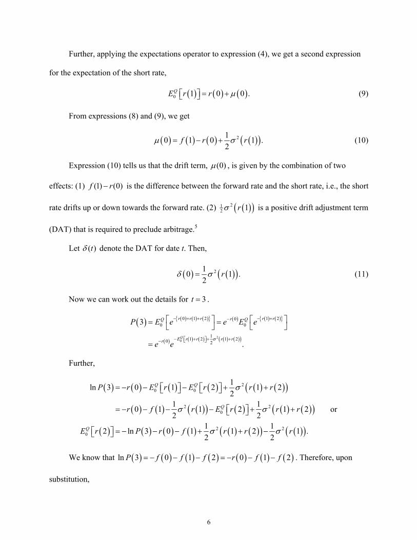
Further, applying the expectations operator to expression (4), we get a second expression
for the expectation of the short rate,
(9) ( ) ( ) ( )0 1 0QE r r µ= + 0 .
From expressions (8) and (9), we get
( ) ( ) ( ) ( )(210 1 0 12
f r rµ = − + ).σ (10)
Expression (10) tells us that the drift term, , is given by the combination of two
effects: (1) is the difference between the forward rate and the short rate, i.e., the short
rate drifts up or down towards the forward rate. (2)
(0)µ
(1) (0)f r−
( )(2 1r )12σ is a positive drift adjustment term
(DAT) that is required to preclude arbitrage.5
Let (δ denote the DAT for date t. Then, )t
( ) ( )(2102
rδ σ= )1 . (11)
Now we can work out the details for . 3t =
( ) ( ) ( ) ( ){ } ( ) ( ) ( ){ }
( ) ( ) ( ) ( ) ( )( )20
0 1 2 1 200 0
11 2 1 20 2
3
.Q
r r r r rrQ Q
E r r r rr
P E e e E e
e eσ
− + + − +−
− + + + −
= =
=
Further,
( ) ( ) ( ) ( ) ( ) ( )( )
( ) ( ) ( )( ) ( ) ( ) ( )( )
( ) ( ) ( ) ( ) ( ) ( )( ) ( )( )
20 0
2 20
2 20
1ln 3 0 1 2 1 22
1 10 1 1 2 1 2 or2 2
1 12 ln 3 0 1 1 2 1 .2 2
Q Q
Q
Q
P r E r E r r r
r f r E r r r
E r P r f r r r
σ
σ σ
σ σ
= − − − + +
= − − − − + +
= − − − + + −
We know that ln . Therefore, upon
substitution,
( ) ( ) ( ) ( ) ( ) ( ) ( )3 0 1 2 0 1 2P f f f r f f= − − − = − − −
6

( ) ( ) ( ) ( )( ) ( )(20
1 12 2 1 2 12 2
QE r f r r rσ σ= + + − )2 . (12)
Thus, the expectation at date 0 of the short rate at date 2 is the forward rate plus a term
determined by the variance, ( ) ( )( ) ( )( )2 21 12 21 2 1r r rσ σ+ − .
Further, applying the expectations operator to expression (4), we get a second expression
for the expectation of the short rate,
(13) ( ) ( ) ( ) ( )0 2 0 0QE r r µ µ= + + 1 .
From expressions (12) and (13), we get
( ) ( ) ( ) ( ) ( ) ( )( ) ( )( )2 21 11 2 0 0 1 2 12 2
f r r r rµ µ σ= − − + + − .σ
Substitute expression (10) above to get:
( ) ( ) ( ) ( ) ( )( ) ( )(211 2 1 1 2 12
f f r r rµ σ= − + + − )2 .σ (14)
Expression (14) tells us that the drift term, , is given by the combination of two
effects: (1) is the difference between the forward rate at date 2 and the forward rate
at date 1, i.e., the nearby forward short rate drifts up or down towards the distant forward rate.
(2)
(1)µ
(2) (1)f f−
( ) ( )( )2 1 2r rσ + − ( )(12 1rσ )2 is a positive drift adjustment term (DAT) that is required to
preclude arbitrage.
Let (1)δ denote the DAT for date 1. Then,
( ) ( ) ( )( ) ( )(211 1 22
r r rδ σ σ= + − )2 1 . (15)
If we add expressions for and (expressions (11) and (15)) we get ( )0δ ( )1δ
( ) ( )( ) ( ) ( )( ) ( )( )
( ) ( )( ) ( )( )
12 2 2
0
2 2
1 11 1 22 21 11 2 1 .2 2
tt r r r r
r r r
δ σ σ σ
σ σ
=
= + + −
= + −
∑ 1
7
If we add expressions for and (expressions (10) and (14)) we get ( )0µ ( )1µ
( ) ( ) ( ) ( ) ( )( ) ( ) ( ) ( ) ( )( ) ( )( )
( ) ( ) ( ) ( )( ) ( )( )
2 2
2 2
1 10 1 1 0 1 2 1 1 2 12 21 12 0 1 2 1 ,2 2
f r r f f r r r
f r r r r
µ µ σ σ σ
σ σ
+ = − + + − + + −
= − + + −
2
.δ∑
which can be simplified to
(16) ( ) ( ) ( ) ( )1 1
0 02 0
t tt f r tµ
= =
= − +∑
Now we can work out the details for . 4t =
( ) ( ) ( ) ( ) ( ){ } ( ) ( ) ( ) ( ){ }
( ) ( ) ( ) ( ) ( ) ( ) ( )( )20
0 1 2 3 1 2 300 0
11 2 3 1 2 30 2
4
.Q
r r r r r r rrQ Q
E r r r r r rr
P E e e E e
e eσ
− + + + − + +−
− + + + + + −
= =
=
Further,
( ) ( ) ( ) ( ) ( ) ( ) ( ) ( )( )
( ) ( ) ( )( ) ( ) ( ) ( )( ) ( )( ) ( )
( ) ( ) ( )( )
( ) ( ) ( ) ( ) ( ) ( ) ( ) ( )( ) ( ) ( )( )
20 0 0
2 2 20
2
2 20
1ln 4 0 1 2 3 1 2 32
1 1 10 1 1 2 1 2 r 1 32 2 2
1 + 1 2 3 or2
1 13 ln 4 0 1 2 1 2 3 1 22 2
Q Q Q
Q
Q
P r E r E r E r r r r
r f r f r r E r
r r r
E r P r f f r r r r r
σ
σ σ σ
σ
σ σ
= − − − − + + +
= − − − − − + + −
+ +
= − − − − + + + − + .
We know that ln .
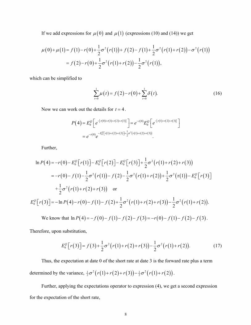
Therefore, upon substitution,
( ) ( ) ( ) ( ) ( ) ( ) ( ) ( ) ( )4 0 1 2 3 0 1 2 3P f f f f r f f f= − − − − = − − − −
( ) ( ) ( ) ( ) ( )( ) ( ) ( )(2 20
1 13 3 1 2 3 1 22 2
QE r f r r r r rσ σ= + + + − + ). (17)
Thus, the expectation at date 0 of the short rate at date 3 is the forward rate plus a term
determined by the variance, ( ) ( ) ( )( ) ( ) ( )( )2 21 12 21 2 3 1 2r r r r rσ σ+ + − + .
Further, applying the expectations operator to expression (4), we get a second expression
for the expectation of the short rate,
8

(18) ( ) ( ) ( ) ( ) ( )0 3 0 0 1QE r r µ µ µ= + + + 2 .
From expressions (17) and (18), we get
( ) ( ) ( ) ( ) ( ) ( ) ( ) ( )( ) ( ) ( )( ) ( )( )2 21 12 3 0 0 1 1 2 3 1 2 12 2
f r r r r r r rµ µ µ σ σ= − − − + + + + + − 21 .2σ
Substitute expressions (10) and (14) above to get:
( ) ( ) ( ) ( ) ( ) ( )( ) ( ) ( )( ) ( )(2 21 12 3 2 1 2 3 1 2 12 2
f f r r r r r rµ σ σ= − + + + − + + )2 .σ (19)
Expression (19) tells us that the drift term, , is given by the combination of two
effects: (1) is the difference between the forward rate at date 3 and the forward rate
at date 2, i.e., the second nearby forward short rate drifts up or down towards the distant forward
rate. (2)
(2)µ
(3) (2)f f−
( ) ( ) ( )( ) ( ) ( )( ) ( )(2 23 1 1r r rσ σ+ + − + + )2σ1 12 22r1 2r r is a positive drift adjustment
term (DAT) that is required to preclude arbitrage.
Let (δ denote the DAT for date 2. Then, )2
( ) ( ) ( ) ( )( ) ( ) ( )( ) ( )(2 21 12 1 2 3 1 22 2
r r r r r rδ σ σ σ= + + − + + )2 1 . (20)
If we add expressions for , and (expressions (11), (15) and (20)) we get ( )0δ ( )1δ ( )2δ
( ) ( ) ( )( ) ( )( ) ( ) ( ) ( )( )
( ) ( )( ) ( )( )
( ) ( ) ( )( ) ( ) ( )( )
22 2 2
0
2 2
2 2
1 1 11 2 1 1 2 32 2 2
1 1 2 12
1 11 2 3 1 2 .2 2
tt r r r r r r
r r r
r r r r r
δ σ σ σ
σ σ
σ σ
=
= + − + + +
− + +
= + + − +
∑
If we add expressions for , and (expressions (10), (14) and (19)) we get ( )0µ ( )1µ ( )2µ
9
( ) ( ) ( ) ( ) ( ) ( ) ( )( ) ( )( ) ( ) ( )
( ) ( ) ( )( ) ( ) ( )( ) ( )( )
( ) ( ) ( ) ( ) ( )( ) ( ) ( )( )
2 2
2 2
2 2
1 10 1 2 2 0 1 2 1 32 2
1 11 2 3 1 2 12 2
1 13 0 1 2 3 1 22 2
f r r r r f f
r r r r r r
f r r r r r r
µ µ µ σ σ
σ σ σ
σ σ
+ + = − + + − + −
+ + + − + +
= − + + + − +
2
2
,
.δ∑
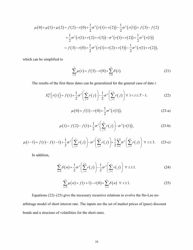
which can be simplified to
(21) ( ) ( ) ( ) ( )2 2
0 03 0
t tt f r tµ
= =
= − +∑
The results of the first three dates can be generalized for the general case of date t.
( ) ( ) ( ) ( )1
2 20
1 1
1 1 12 2
t tQ
j jE r t f t r j r j t Tσ σ
−
= =
= + − ∀ < ≤ −
∑ ∑ 1. (22)
( ) ( ) ( ) ( )(210 1 0 12
f r rµ = − + ) ,σ (23-a)
( ) ( ) ( ) ( ) ( )(2
2 2
1
11 2 1 12 j
f f r j rµ σ=
= − + −
∑ ) ,σ (23-b)
( ) ( ) ( ) ( ) ( ) ( )1 2
2 2 2
1 1 1 1
1 11 1 3.2 2
t t t n
j j n jt f t f t r j r j r j tµ σ σ σ
− −
= = = =
− = − − + − + ∀ ≥
∑ ∑ ∑ ∑ (23-c)
In addition,
( ) ( ) ( )1
2 2
0 1 1
1 1 1.2 2
t t t
n j jn r j r jδ σ σ
+
= = =
= −
∑ ∑ ∑ t∀ ≥ (24)
(25) ( ) ( ) ( ) ( )0 1
1 0 1.t t
n nn f t r n tµ δ
= =
= + − + ∀ ≥∑ ∑
Equations (22)–(25) give the necessary recursive relations to evolve the Ho-Lee no-
arbitrage model of short interest rate. The inputs are the set of market prices of (pure) discount
bonds and a structure of volatilities for the short rates.
10

The above discussion is general in the sense that it applies equally well to implementation
based on the binomial models and Monte Carlo simulation. If we adopt the tree approach to
depict the evolution, we would write the evolutionary equation as
( )( ) ( ) ( )( ) ( ) ( )
12
12
with probability
with probability ,
r t t t t t t t tr t
r t t t t t t t t
µ σ
µ σ
− ∆ + − ∆ ∆ + − ∆ ∆= − ∆ + − ∆ ∆ − − ∆ ∆
(26)
or in the case of , 1t∆ =
( )( ) ( ) ( )( ) ( ) ( )
12
12
1 1 1 with probability
1 1 1 with probability .
r t t tr t
r t t t
µ σ
µ σ
− + − + −= − + − − −
(27)
Thus, for t , 1=
( ) ( ) ( ) ( )( ) ( ) ( ) ( )
11 2
10 2
1 0 0 0 with probability ,
1 0 0 0 with probability ,
r r
r r
µ σ
µ σ
= + +
= + − (28)
where denotes the nth node at date t.( )nr t 6
And, for 2,t =
( ) ( ) ( ) ( )( ) ( ) ( ) ( ) ( )
( ) ( ) ( ) ( )( )( ) ( ) ( ) ( ) ( )
13 0 2
12 0 2
2 1 1 1 with probability
0 0 1 0 1 ,
2 1 1 1 with probability
0 0 1 0 1 .
r r
r
r r r
r
µ σ
µ µ σ σ
µ σ
µ µ σ σ
= + +
= + + + +
= + −
= + + + −
(29-a)
and
( ) ( ) ( ) ( )( ) ( ) ( ) ( ) ( )
( ) ( ) ( ) ( )( )( ) ( ) ( ) ( ) ( )
11 1 2
10 1 2
2 1 1 1 with probability
0 0 1 0 1 ,
2 1 1 1 with probability
0 0 1 0 1 .
r r
r
r r r
r
µ σ
µ µ σ σ
µ σ
µ µ σ σ
= + +
= + + − +
= + −
= + + − −
(29-b)
The progression to the next date should be clear. See Figure 1-A for an example of a tree
and Figure 2-A for an example of a lattice.
11
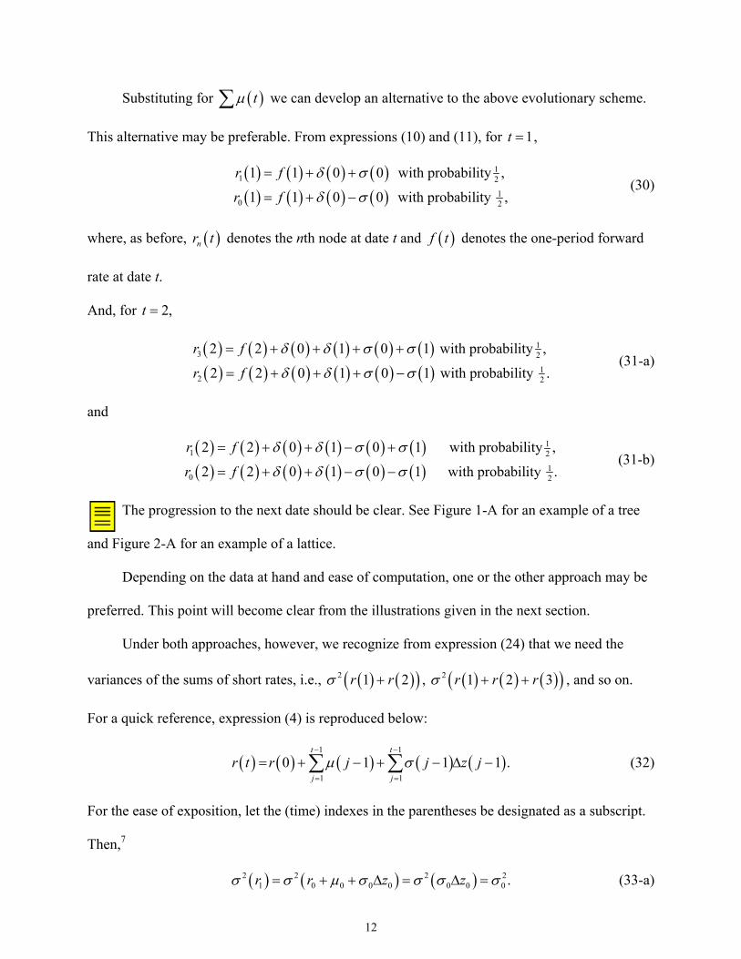
Substituting for (µ∑ we can develop an alternative to the above evolutionary scheme.
This alternative may be preferable. From expressions (10) and (11), for t ,
)t
1=
( ) ( ) ( ) ( )( ) ( ) ( ) ( )
11 2
10 2
1 1 0 0 with probability ,
1 1 0 0 with probability ,
r f
r f
δ σ
δ σ
= + +
= + − (30)
where, as before, r t denotes the nth node at date t and denotes the one-period forward
rate at date t.
( )n ( )f t
And, for 2,t =
( ) ( ) ( ) ( ) ( ) ( )( ) ( ) ( ) ( ) ( ) ( )
13 2
12 2
2 2 0 1 0 1 with probability ,
2 2 0 1 0 1 with probability .
r f
r f
δ δ σ σ
δ δ σ σ
= + + + +
= + + + − (31-a)
and
( ) ( ) ( ) ( ) ( ) ( )( ) ( ) ( ) ( ) ( ) ( )
11 2
10 2
2 2 0 1 0 1 with probability ,
2 2 0 1 0 1 with probability .
r f
r f
δ δ σ σ
δ δ σ σ
= + + − +
= + + − − (31-b)
The progression to the next date should be clear. See Figure 1-A for an example of a tree
and Figure 2-A for an example of a lattice.
Depending on the data at hand and ease of computation, one or the other approach may be
preferred. This point will become clear from the illustrations given in the next section.
Under both approaches, however, we recognize from expression (24) that we need the
variances of the sums of short rates, i.e., , , and so on.
For a quick reference, expression (4) is reproduced below:
( ) ( )( )2 1 2r rσ + ( ) ( ) ( )( )2 1 2 3r r rσ + +
(32) ( ) ( ) ( ) ( ) (1 1
1 10 1 1
t t
j jr t r j j z jµ σ
− −
= =
= + − + − ∆ −∑ ∑ )1 .
20σ
For the ease of exposition, let the (time) indexes in the parentheses be designated as a subscript.
Then,7
(33-a) ( ) ( ) ( )2 2 21 0 0 0 0 0 0 .r r z zσ σ µ σ σ σ= + + ∆ = ∆ =
12

(33-b)
( ) (( ) (( ) ( ) (
2 21 2 0 0 0 0 0 0 1 0 0 1 1
2 20 0 0 0 1 1 0 0 1 1
2 20 0 1 1 0 0 1 1
2 20 1
2
2 2Cov 2
4 .
r r r z r z z
z z z z
z z z
σ σ µ σ µ µ σ σ
σ σ σ σ σ σ σ
σ σ σ σ σ σ
σ σ
+ = + + ∆ + + + + ∆ + ∆
= ∆ + ∆ + ∆ = ∆ + ∆
= ∆ + ∆ + ∆ ∆
= +
))),
z
z
)
)
z
2 2σ σ
t −
∀
(33-c)
( ) (( )( ) ( ) ( )
( ) (( )
2 21 2 3 0 0 0 0 1 1 0 0 1 1 2 2
20 0 1 1 2 2
2 2 20 0 1 1 2 2
0 0 1 1 0 0 2 2
1 1 2 2
2 2 20 1 2
3 2
3 2
2Cov 3 ,2 2Cov 3 ,
2Cov 2 , ,
9 4 .
r r r z z z z z
z z z
z z z
z z z z
z z
σ σ σ σ σ σ σ σ
σ σ σ σ
σ σ σ σ σ σ
σ σ σ σ
σ σ
σ σ σ
+ + = ∆ + ∆ + ∆ + ∆ + ∆ + ∆
= ∆ + ∆ + ∆
= ∆ + ∆ + ∆
+ ∆ ∆ + ∆ ∆
+ ∆ ∆
= + +
Therefore, in general,
(34) ( ) ( )
( )
2 21 1
1 1
2 21
1
1
1 .
t t
k kj k
t
kk
r j t k z
t k
σ σ σ
σ
− −= =
−=
= − + ∆
= − +
∑ ∑
∑
For example, expression (34) will yield for t , 4=
( )2 2 21 2 3 4 0 1 2 316 9 4 .r r r rσ σ σ+ + + = + + +
Implementation of expression (34) can be made easier if we use matrix notation. Let
denote a diagonal t matrix whose elements are . Let denote a t-
dimensional column vector whose elements are the integer values of the index t in reverse order.
Then, expression (34) can be written as
tD
t× 21 1jj ja jσ −= ∀ ≤ tw
(35) ( )2 T
1 ,
t
t t tj
r j tσ=
=
∑ w D w
where T denotes transposition.
For example, expression (35) will yield for t , 4=
13
[ ]
20
242 T 1
4 4 4 21 2
23
2 2 2 20 1 2 3
40 0 030 0 0
4 3 2 120 0 010 0 0
16 9 4 .
jj
r
σσ
σσ
σ
σ σ σ σ
=
= =
= + + +
∑ w D w
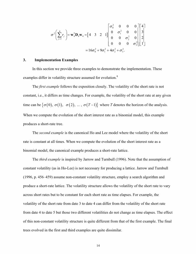
3. Implementation Examples
In this section we provide three examples to demonstrate the implementation. These
examples differ in volatility structure assumed for evolution.8
The first example follows the exposition closely. The volatility of the short rate is not
constant, i.e., it differs as time changes. For example, the volatility of the short rate at any given
time can be { where T denotes the horizon of the analysis.
When we compute the evolution of the short interest rate as a binomial model, this example
produces a short-rate tree.
( ) ( )0 , 1 ,σ σ ( ) ( )}2 , ... , 1Tσ σ −
The second example is the canonical Ho and Lee model where the volatility of the short
rate is constant at all times. When we compute the evolution of the short interest rate as a
binomial model, the canonical example produces a short-rate lattice.
The third example is inspired by Jarrow and Turnbull (1996). Note that the assumption of
constant volatility (as in Ho-Lee) is not necessary for producing a lattice. Jarrow and Turnbull
(1996, p. 456–459) assume non-constant volatility structure, employ a search algorithm and
produce a short-rate lattice. The volatility structure allows the volatility of the short rate to vary
across short rates but to be constant for each short rate as time elapses. For example, the
volatility of the short rate from date 3 to date 4 can differ from the volatility of the short rate
from date 4 to date 5 but those two different volatilities do not change as time elapses. The effect
of this non-constant volatility structure is quite different from that of the first example. The final
trees evolved in the first and third examples are quite dissimilar.
14
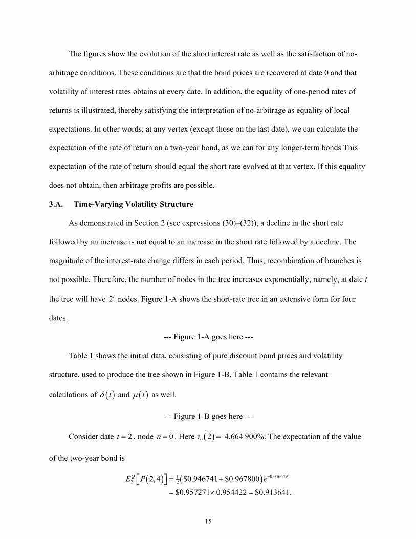
The figures show the evolution of the short interest rate as well as the satisfaction of no-
arbitrage conditions. These conditions are that the bond prices are recovered at date 0 and that
volatility of interest rates obtains at every date. In addition, the equality of one-period rates of
returns is illustrated, thereby satisfying the interpretation of no-arbitrage as equality of local
expectations. In other words, at any vertex (except those on the last date), we can calculate the
expectation of the rate of return on a two-year bond, as we can for any longer-term bonds This
expectation of the rate of return should equal the short rate evolved at that vertex. If this equality
does not obtain, then arbitrage profits are possible.
3.A. Time-Varying Volatility Structure
As demonstrated in Section 2 (see expressions (30)–(32)), a decline in the short rate
followed by an increase is not equal to an increase in the short rate followed by a decline. The
magnitude of the interest-rate change differs in each period. Thus, recombination of branches is
not possible. Therefore, the number of nodes in the tree increases exponentially, namely, at date t
the tree will have 2 nodes. Figure 1-A shows the short-rate tree in an extensive form for four
dates.
t
--- Figure 1-A goes here ---
Table 1 shows the initial data, consisting of pure discount bond prices and volatility
structure, used to produce the tree shown in Figure 1-B. Table 1 contains the relevant
calculations of and as well. ( )tδ ( )tµ
--- Figure 1-B goes here ---
Consider date 2t = , node . Here 4.664 900%. The expectation of the value
of the two-year bond is
0n = ( )0 2r =
( ) ( ) 0.04664912 22,4 $0.946741 $0.967800
$0.957271 0.954422 $0.913641.
QE P e−= + = × =
15
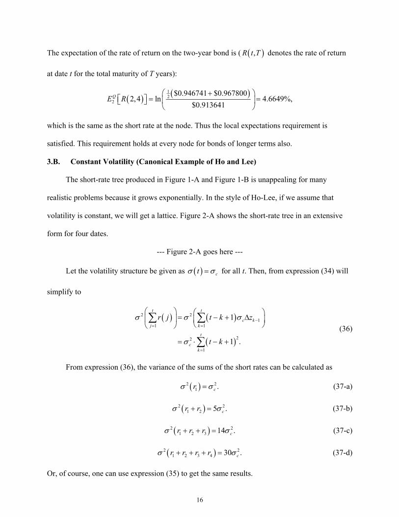
The expectation of the rate of return on the two-year bond is ( denotes the rate of return
at date t for the total maturity of T years):
( ,R t T )
( ) ( )12
2
$0.946741 $0.9678002,4 ln 4.6649%,
$0.913641QE R
+ = =
which is the same as the short rate at the node. Thus the local expectations requirement is
satisfied. This requirement holds at every node for bonds of longer terms also.
3.B. Constant Volatility (Canonical Example of Ho and Lee)
The short-rate tree produced in Figure 1-A and Figure 1-B is unappealing for many
realistic problems because it grows exponentially. In the style of Ho-Lee, if we assume that
volatility is constant, we will get a lattice. Figure 2-A shows the short-rate tree in an extensive
form for four dates.
--- Figure 2-A goes here ---
Let the volatility structure be given as for all t. Then, from expression (34) will
simplify to
( ) ctσ =σ
2σ
2.σ
2σ
2σ
(36) ( ) ( )
( )
2 21
1 1
22
1
1
1 .
t t
c kj k
t
ck
r j t k z
t k
σ σ σ
σ
−= =
=
= − + ∆
= ⋅ − +
∑ ∑
∑
From expression (36), the variance of the sums of the short rates can be calculated as
(37-a) ( )21 .crσ =
(37-b) ( )21 2 5 cr rσ + =
(37-c) ( )21 2 3 14 .cr r rσ + + =
(37-d) ( )21 2 3 4 30 .cr r r rσ + + + =
Or, of course, one can use expression (35) to get the same results.
16
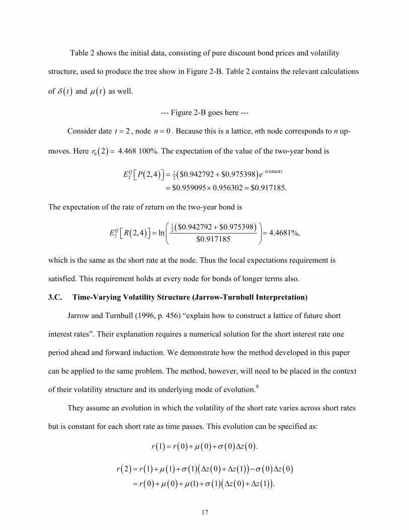
Table 2 shows the initial data, consisting of pure discount bond prices and volatility
structure, used to produce the tree show in Figure 2-B. Table 2 contains the relevant calculations
of and as well. ( )tδ ( )tµ
--- Figure 2-B goes here ---
Consider date 2t = , node . Because this is a lattice, nth node corresponds to n up-
moves. Here 4.468 100%. The expectation of the value of the two-year bond is
0n =
( )0 2r =
( ) ( ) 0.04468112 22,4 $0.942792 $0.975398
$0.959095 0.956302 $0.917185.
QE P e−= + = × =
The expectation of the rate of return on the two-year bond is
( ) ( )12
2
$0.942792 $0.9753982,4 ln 4.4681%,
$0.917185QE R
+ = =
which is the same as the short rate at the node. Thus the local expectations requirement is
satisfied. This requirement holds at every node for bonds of longer terms also.
3.C. Time-Varying Volatility Structure (Jarrow-Turnbull Interpretation)
Jarrow and Turnbull (1996, p. 456) “explain how to construct a lattice of future short
interest rates”. Their explanation requires a numerical solution for the short interest rate one
period ahead and forward induction. We demonstrate how the method developed in this paper
can be applied to the same problem. The method, however, will need to be placed in the context
of their volatility structure and its underlying mode of evolution.9
They assume an evolution in which the volatility of the short rate varies across short rates
but is constant for each short rate as time passes. This evolution can be specified as:
( ) ( ) ( ) ( ) ( )1 0 0 0 0r r zµ σ= + + ∆ .
0
z
( ) ( ) ( ) ( ) ( ) ( )( ) ( ) ( )( ) ( ) ( ) ( ) ( )( )
2 1 1 1 0 1 0
0 0 (1) 1 0 1 .
r r z z z
r z
µ σ σ
µ µ σ
= + + ∆ + ∆ − ∆
= + + + ∆ + ∆
17
( ) ( ) ( ) ( ) ( ) ( ) ( )( ) ( ) ( ) ( )( )
( ) ( ) ( ) ( ) ( ) ( ) ( )( )3 2 2 2 0 1 2 1 0 1
0 0 (1) 2 2 0 1 2 .
r r z z z z z
r z z
µ σ σ
µ µ µ σ
= + + ∆ + ∆ + ∆ − ∆ + ∆
= + + + + ∆ + ∆ + ∆z
z
.
20σ
z
.j kσ σ
3σ
( ) ( ) ( ) ( ) ( ) ( ) ( ) ( )( ) ( ) ( ) ( ) ( )( )
( ) ( ) ( ) ( ) ( ) ( ) ( ) ( ) ( )( )4 3 3 3 0 1 2 3 1 0 1 2
0 0 (1) 2 3 3 0 1 2 3 .
r r z z z z z z z
r z z z
µ σ σ
µ µ µ µ σ
= + + ∆ + ∆ + ∆ + ∆ − ∆ + ∆ + ∆
= + + + + + ∆ + ∆ + ∆ + ∆
In general, then,
(38) ( ) ( ) ( ) ( ) ( )1 1
0 00 1
t t
j jr t r j t z jµ σ
− −
= =
= + + − ∆∑ ∑
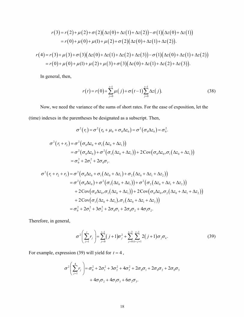
Now, we need the variance of the sums of short rates. For the ease of exposition, let the
(time) indexes in the parentheses be designated as a subscript. Then,
( ) ( ) ( )2 2 21 0 0 0 0 0 0 .r r z zσ σ µ σ σ σ= + + ∆ = ∆ =
( ) ( )( )( ) ( )( ) ( )( )
2 21 2 0 0 1 0 1
2 20 0 1 0 1 0 0 1 0 1
2 20 1 0 1
2Cov ,
2 2 .
r r z z z
z z z z z
σ σ σ σ
σ σ σ σ σ σ
σ σ σ σ
+ = ∆ + ∆ + ∆
= ∆ + ∆ + ∆ + ∆ ∆ + ∆
= + +
( ) ( ) ( )( )( ) ( )( ) ( )( )
( )( ) ( )( )( ) ( )( )
2 21 2 3 0 0 1 0 1 2 0 1 2
2 2 20 0 1 0 1 2 0 1 2
0 0 1 0 1 0 0 2 0 1 2
1 0 1 2 0 1 2
2 2 20 1 2 0 1 0 2 1 2
2Cov , 2Cov ,
2Cov ,
2 3 2 2 4 .
r r r z z z z z z
z z z z z z
z z z z z z z
z z z z z
σ σ σ σ σ
σ σ σ σ σ σ
σ σ σ σ
σ σ
σ σ σ σ σ σ σ σ σ
+ + = ∆ + ∆ + ∆ + ∆ + ∆ + ∆
= ∆ + ∆ + ∆ + ∆ + ∆ + ∆
+ ∆ ∆ + ∆ + ∆ ∆ + ∆ + ∆
+ ∆ + ∆ ∆ + ∆ + ∆
= + + + + +
Therefore, in general,
(39) ( ) ( )1 2 1
2 2
1 0 0 11 2 1
t t t t
j jj j j k j
r j jσ σ− − −
= = = = +
= + + +
∑ ∑ ∑ ∑
For example, expression (39) will yield for t , 4=
42 2 2 2 2
0 1 2 3 0 1 0 2 01
1 2 1 3 2 3
2 3 4 2 2 2
4 4 6 .
jj
rσ σ σ σ σ σ σ σ σ σ
σ σ σ σ σ σ=
= + + + + + +
+ + +
∑
18
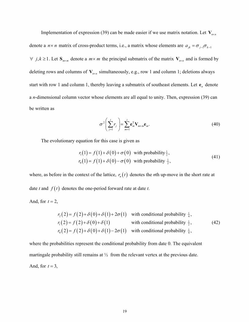
Implementation of expression (39) can be made easier if we use matrix notation. Let
denote a matrix of cross-product terms, i.e., a matrix whose elements are a
. Let S denote a the principal submatrix of the matrix and is formed by
deleting rows and columns of V simultaneously, e.g., row 1 and column 1; deletions always
start with row 1 and column 1, thereby leaving a submatrix of southeast elements. Let e denote
a n-dimensional column vector whose elements are all equal to unity. Then, expression (39) can
be written as
n n×V
1 1k− −n n×
1≥
jk jσ σ=
n
n
,j k∀ m m× m m×
n n×
n×V
(40) 2 T
1 1.
t t
j m m mj m
rσ ×= =
=
∑ ∑e V em
The evolutionary equation for this case is given as
( ) ( ) ( ) ( )( ) ( ) ( ) ( )
11 2
10 2
1 1 0 0 with probability ,
1 1 0 0 with probability ,
r f
r f
δ σ
δ σ
= + +
= + − (41)
where, as before in the context of the lattice, denotes the nth up-move in the short rate at
date t and denotes the one-period forward rate at date t.
( )nr t
( )f t
And, for 2,t =
( ) ( ) ( ) ( ) ( )( ) ( ) ( ) ( )( ) ( ) ( ) ( ) ( )
12 4
11 2
10 4
2 2 0 1 2 1 with conditional probability ,
2 2 0 1 with conditional probability ,
2 2 0 1 2 1 with conditional probability ,
r f
r f
r f
δ δ σ
δ δ
δ δ σ
= + + +
= + +
= + + −
(42)
where the probabilities represent the conditional probability from date 0. The equivalent
martingale probability still remains at ½ from the relevant vertex at the previous date.
And, for 3,t =
19

( ) ( ) ( ) ( )
( ) ( ) ( ) ( )
( ) ( ) ( ) ( )
( ) ( ) ( ) ( )
21
3 80
23
2 80
23
1 80
21
0 80
3 3 3 2 with conditional probability ,
3 3 2 with conditional probability ,
3 3 2 with conditional probability ,
3 3 3 2 with conditional probability ,
j
j
j
j
r f j
r f j
r f j
r f j
δ σ
δ σ
δ σ
δ σ
=
=
=
=
= + +
= + +
= + −
= + −
∑
∑
∑
∑
(43)
where the interpretation of the probability is as given for the preceding expression.
The progression to the next date should be clear. Figure 3-A shows the short-rate tree in an
extensive form for four dates.
--- Figure 3-A goes here ---
Table 3 shows the initial data, consisting of pure discount bond prices and volatility
structure, used to produce the tree show in Figure 3-B. These data are the same as used by Jarrow
and Turnbull. Table 3 contains the relevant calculations of and as well. ( )tδ ( )tµ
--- Figure 3-B goes here ---
Consider date 2t = , node . Because this is a lattice, nth node corresponds to n up-
moves. Here 4.858 300%. The expectation of the value of the two-year bond is
0n =
( )0 2r =
( ) ( ) 0.04858312 22,4 $0.937717 $0.958575
$0.948146 0.952578 $0.903183.
QE P e−= + = × =
The expectation of the rate of return on the one-year bond is
( ) ( )12
2
$0.937717 $0.9585752,4 ln 4.8583%,
$0.903183QE R
+ = =
which is the same as the short rate at the node. Thus the local expectations requirement is
satisfied. This requirement holds at every node for bonds of longer terms.
20
4. Concluding Remarks
Ho and Lee’s interest-rate model retains the distinction of being the first no-arbitrage
model that can be calibrated to market data. One of the major short-comings, however, has been
the complexity of its discrete time implementation. In general, it has required numerical methods
and forward induction. In this paper we have analytically demonstrated its implementation. It is
relatively straightforward to identify recursive expressions for short rates at all (nodes and) dates.
Armed with a set of expressions, we can map out the entire evolution. It is advisable to
remember that the objective of the paper was to demonstrate the implementation of the Ho-Lee
model in discrete time and not necessarily discuss the evolution of interest rates under different
specifications of the volatility function. Whether the evolution will result in a tree or a lattice will
depend on the volatility structure assumed for short rates. Even for a complex interpretation of
the volatility structure, the proposed method eliminates the numerical search or optimization
process. This implementation has an added advantage of being scalable, such that once the
longest-maturity is known we can use matrix algebra for intermediate calculations. Lastly we
reëmphasize that this method of implementation applies to both binomial models and Monte
Carlo simulation of interest rates.
21
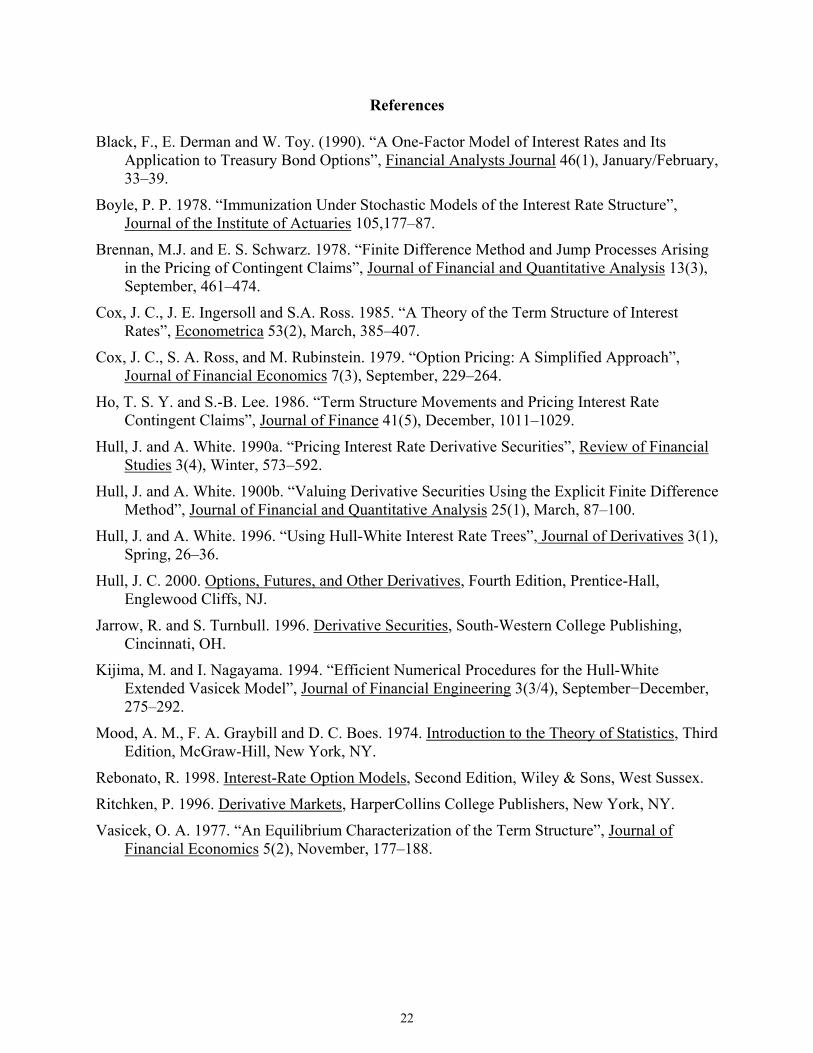
References
Black, F., E. Derman and W. Toy. (1990). “A One-Factor Model of Interest Rates and Its Application to Treasury Bond Options”, Financial Analysts Journal 46(1), January/February, 33–39.
Boyle, P. P. 1978. “Immunization Under Stochastic Models of the Interest Rate Structure”, Journal of the Institute of Actuaries 105,177–87.
Brennan, M.J. and E. S. Schwarz. 1978. “Finite Difference Method and Jump Processes Arising in the Pricing of Contingent Claims”, Journal of Financial and Quantitative Analysis 13(3), September, 461–474.
Cox, J. C., J. E. Ingersoll and S.A. Ross. 1985. “A Theory of the Term Structure of Interest Rates”, Econometrica 53(2), March, 385–407.
Cox, J. C., S. A. Ross, and M. Rubinstein. 1979. “Option Pricing: A Simplified Approach”, Journal of Financial Economics 7(3), September, 229–264.
Ho, T. S. Y. and S.-B. Lee. 1986. “Term Structure Movements and Pricing Interest Rate Contingent Claims”, Journal of Finance 41(5), December, 1011–1029.
Hull, J. and A. White. 1990a. “Pricing Interest Rate Derivative Securities”, Review of Financial Studies 3(4), Winter, 573–592.
Hull, J. and A. White. 1900b. “Valuing Derivative Securities Using the Explicit Finite Difference Method”, Journal of Financial and Quantitative Analysis 25(1), March, 87–100.
Hull, J. and A. White. 1996. “Using Hull-White Interest Rate Trees”, Journal of Derivatives 3(1), Spring, 26–36.
Hull, J. C. 2000. Options, Futures, and Other Derivatives, Fourth Edition, Prentice-Hall, Englewood Cliffs, NJ.
Jarrow, R. and S. Turnbull. 1996. Derivative Securities, South-Western College Publishing, Cincinnati, OH.
Kijima, M. and I. Nagayama. 1994. “Efficient Numerical Procedures for the Hull-White Extended Vasicek Model”, Journal of Financial Engineering 3(3/4), September−December, 275–292.
Mood, A. M., F. A. Graybill and D. C. Boes. 1974. Introduction to the Theory of Statistics, Third Edition, McGraw-Hill, New York, NY.
Rebonato, R. 1998. Interest-Rate Option Models, Second Edition, Wiley & Sons, West Sussex.
Ritchken, P. 1996. Derivative Markets, HarperCollins College Publishers, New York, NY.
Vasicek, O. A. 1977. “An Equilibrium Characterization of the Term Structure”, Journal of Financial Economics 5(2), November, 177–188.
22

Table 1 Data and Intermediate Calculations for the Interest Rate Tree Shown in Figure 1-B (Time-Varying Volatility) Maturity Years
Bond Price (at date 0)
Short Rate
Volatility
Bond Yield
Forward Rate
Var (Sum (Short Rate))
Sum (Delta)
DAT = Delta
Drift Sum(Drift)
t ( )P t ( )tσ ( )y t ( )f t ( )2
1
t
jr jσ
=
∑ ( )
1
0
t
jjδ
−
=∑ ( )tδ ( )tµ ( )
1
0
t
jjµ
−
=∑ ( )0
QE r t
0 1.7% 6.198 2% 0.014 450% 0.014 450% 0.424 050% 0.424 050% 6.198 200% 1 $0.939 900 1.5% 6.198 2% 6.607 8% 0.000 289 0.054 600% 0.040 150% 1.242 650% 1.666 700% 6.622 250% 2 $0.879 801 1.1% 6.403 0% 7.810 3% 0.001 381 0.112 050% 0.057 450% -0.291 950% 1.374 750% 7.864 900% 3 $0.813 700 6.872 1% 7.460 9% 0.003 622 0.178 363% 0.066 312% 7.572 950% 4 $0.755 201 7.019 3% 0.007 189 Notes: Bond prices are given exogenously. The face value is $1. Bond yields are calculated as . All rates are annual. ( ) ( )( )ln /y t P t t= −
23
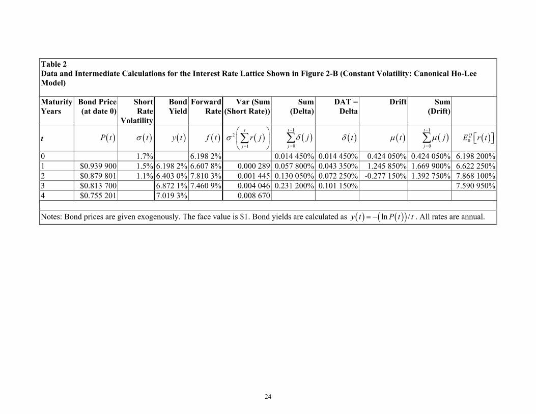
Table 2 Data and Intermediate Calculations for the Interest Rate Lattice Shown in Figure 2-B (Constant Volatility: Canonical Ho-Lee Model) Maturity Years
Bond Price (at date 0)
Short Rate
Volatility
Bond Yield
Forward Rate
Var (Sum (Short Rate))
Sum (Delta)
DAT = Delta
Drift Sum(Drift)
t ( )P t ( )tσ ( )y t (f t ) ( )2
1
t
jr jσ
=
∑ ( )
1
0
t
jjδ
−
=∑ ( )tδ ( )tµ ( )
1
0
t
jjµ
−
=∑ ( )0
QE r t
0 1.7% 6.198 2% 0.014 450% 0.014 450% 0.424 050% 0.424 050% 6.198 200% 1 $0.939 900 1.5% 6.198 2% 6.607 8% 0.000 289 0.057 800% 0.043 350% 1.245 850% 1.669 900% 6.622 250% 2 $0.879 801 1.1% 6.403 0% 7.810 3% 0.001 445 0.130 050% 0.072 250% -0.277 150% 1.392 750% 7.868 100% 3 $0.813 700 6.872 1% 7.460 9% 0.004 046 0.231 200% 0.101 150% 7.590 950% 4 $0.755 201 7.019 3% 0.008 670 Notes: Bond prices are given exogenously. The face value is $1. Bond yields are calculated as . All rates are annual. ( ) ( )( )ln /y t P t t= −
24
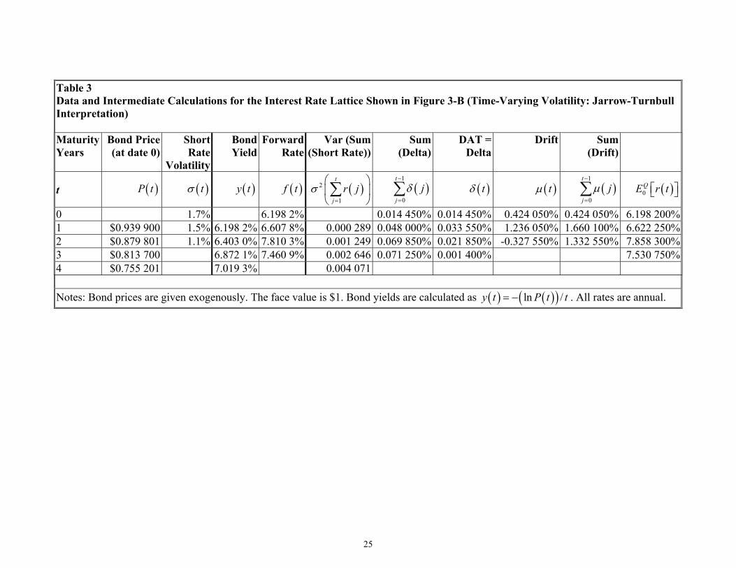
Table 3 Data and Intermediate Calculations for the Interest Rate Lattice Shown in Figure 3-B (Time-Varying Volatility: Jarrow-Turnbull Interpretation) Maturity Years
Bond Price (at date 0)
Short Rate
Volatility
Bond Yield
Forward Rate
Var (Sum (Short Rate))
Sum (Delta)
DAT = Delta
Drift Sum(Drift)
t ( )P t ( )tσ ( )y t (f t ) ( )2
1
t
jr jσ
=
∑ ( )
1
0
t
jjδ
−
=∑ ( )tδ ( )tµ ( )
1
0
t
jjµ
−
=∑ ( )0
QE r t
0 1.7% 6.198 2% 0.014 450% 0.014 450% 0.424 050% 0.424 050% 6.198 200% 1 $0.939 900 1.5% 6.198 2% 6.607 8% 0.000 289 0.048 000% 0.033 550% 1.236 050% 1.660 100% 6.622 250% 2 $0.879 801 1.1% 6.403 0% 7.810 3% 0.001 249 0.069 850% 0.021 850% -0.327 550% 1.332 550% 7.858 300% 3 $0.813 700 6.872 1% 7.460 9% 0.002 646 0.071 250% 0.001 400% 7.530 750% 4 $0.755 201 7.019 3% 0.004 071 Notes: Bond prices are given exogenously. The face value is $1. Bond yields are calculated as . All rates are annual. ( ) ( )( )ln /y t P t t= −
25
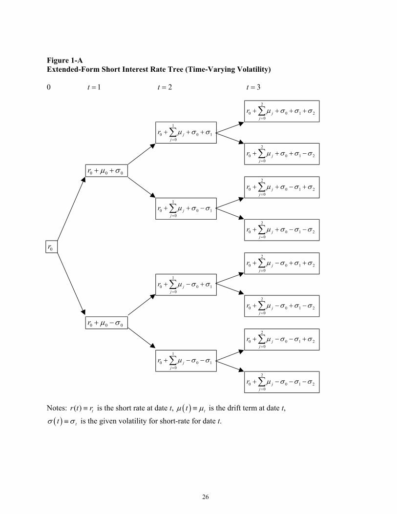
Figure 1-A Extended-Form Short Interest Rate Tree (Time-Varying Volatility) 0 1t = 2t = 3t = 2
0 0 10
jj
r µ σ σ σ=
+ + + +∑ 2
1
0 00
jj
r µ σ σ=
+ + +∑
2
0 0 10
jj
r µ σ σ σ=
+ + + −∑ 2
0 0r µ σ+ + 0 2
0 0 10
jj
r µ σ σ σ=
+ + − +∑ 2
1
0 00
jj
r µ σ σ=
+ + −∑
2
0 00
jj
r µ σ σ σ=
+ + − −∑ 1 2
0r 2
0 0 10
jj
r µ σ σ σ=
+ − + +∑ 2
1
0 00
jj
r µ σ σ=
+ − +∑
2
0 00
jj
r µ σ σ σ=
+ − + −∑ 1 2
0 0 0r µ σ+ − 2
0 00
jj
r µ σ σ σ=
+ − − +∑ 1 2
1
0 00
jj
r µ σ σ=
+ − −∑
2
0 00
jj
r µ σ σ σ=
+ − − −∑ 1 2
Notes: is the short rate at date t, is the drift term at date t,
is the given volatility for short-rate for date t.
( ) tr t r≡
tσ( ) ttµ ≡ µ
( )tσ ≡
1
1
1
1
26
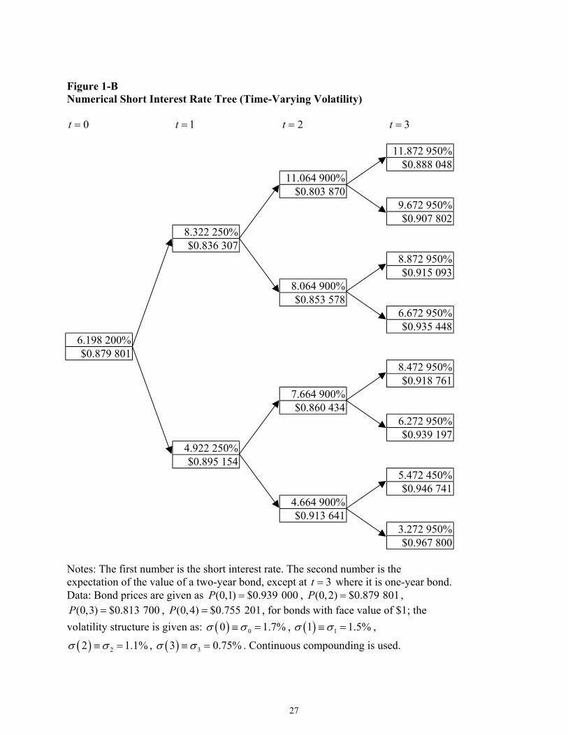
Figure 1-B Numerical Short Interest Rate Tree (Time-Varying Volatility)
0t = 1t = 2t = 3t =
11.872 950% $0.888 048 11.064 900% $0.803 870 9.672 950% $0.907 802 8.322 250% $0.836 307 8.872 950% $0.915 093 8.064 900% $0.853 578 6.672 950% $0.935 448
6.198 200% $0.879 801
8.472 950% $0.918 761 7.664 900% $0.860 434 6.272 950% $0.939 197 4.922 250% $0.895 154 5.472 450% $0.946 741 4.664 900% $0.913 641 3.272 950% $0.967 800
Notes: The first number is the short interest rate. The second number is the expectation of the value of a two-year bond, except at t where it is one-year bond. Data: Bond prices are given as , ,
, , for bonds with face value of $1; the volatility structure is given as: , ,
, . Continuous compounding is used.
3=(0,2P
( )1σ σ
(0,1) $0.939 000P =$0.755 201=
( ) 00 1.7%σ σ≡ =
0.75%
) $0.879 801=
1 1.5%≡ =(0,3) $0.813 700P =
( ) 22 1.1%σ σ≡ =
(0,4)P
( ) 33σ σ≡ =
27

Figure 2-A Extended-Form Short Interest Rate Lattice (Constant Volatility: Canonical Ho-Lee Model) 0 1t = 2t = 3t = 2
00
3j cj
r µ σ=
+ +∑
1
00
2j cj
r µ σ=
+ +∑
0 0 cr µ σ+ +
2
00
j cj
r µ σ=
+ +∑
0r 1
00
jj
r µ=
+∑
0 0 cr µ σ+ −
2
00
j cj
r µ σ=
+ −∑
1
00
2j cj
r µ=
+ −∑ σ
2
00
3j cj
r µ σ=
+ −∑
Notes: is the short rate at date t, is the drift term at date t,
is the given volatility for short-rate for date t.
( ) tr t r≡
tσ( ) ttµ ≡ µ
( )tσ ≡
28
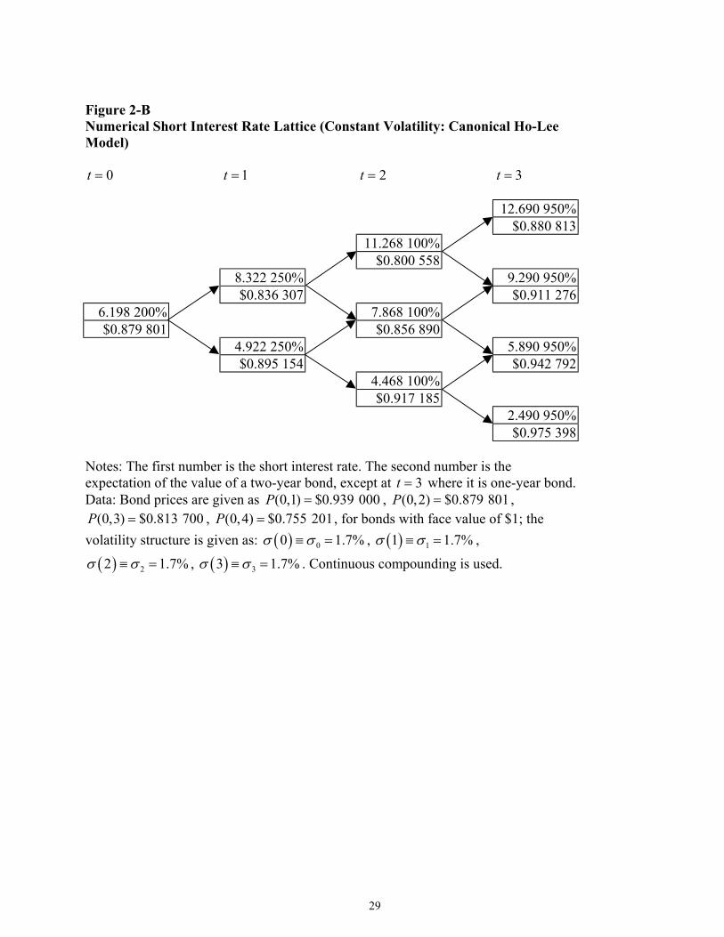
Figure 2-B Numerical Short Interest Rate Lattice (Constant Volatility: Canonical Ho-Lee Model)
0t = 1t = 2t = 3t =
12.690 950% $0.880 813 11.268 100% $0.800 558 8.322 250% 9.290 950% $0.836 307 $0.911 276
6.198 200% 7.868 100% $0.879 801 $0.856 890
4.922 250% 5.890 950% $0.895 154 $0.942 792 4.468 100% $0.917 185 2.490 950% $0.975 398
Notes: The first number is the short interest rate. The second number is the expectation of the value of a two-year bond, except at t where it is one-year bond. Data: Bond prices are given as , ,
, , for bonds with face value of $1; the volatility structure is given as: , ,
, . Continuous compounding is used.
3=(0,2P
( )1σ σ
(0,1) $0.939 000P =$0.755 201=
( ) 00 1.7%σ σ≡ =
1.7%
) $0.879 801=
1 1.7%≡ =(0,3) $0.813 700P =
( ) 22 1.7%σ σ≡ =
(0,4)P
( ) 33σ σ≡ =
29
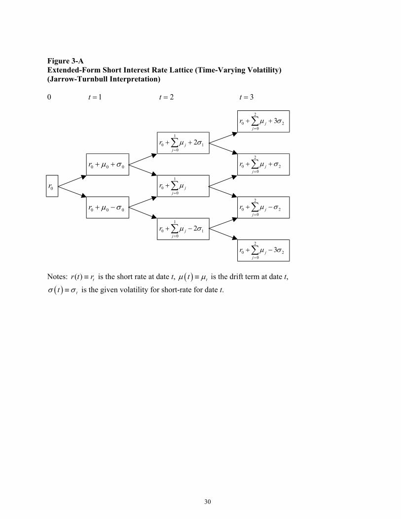
Figure 3-A Extended-Form Short Interest Rate Lattice (Time-Varying Volatility) (Jarrow-Turnbull Interpretation) 0 1t = 2t = 3t = 2
0 20
3jj
r µ σ=
+ +∑
1
0 10
2jj
r µ σ=
+ +∑
0 0r µ σ+ +
2
0 20
jj
r µ σ=
+ +∑
0r 1
00
jj
r µ=
+∑
0 0 0r µ σ+ −
2
0 20
jj
r µ σ=
+ −∑
1
0 10
2jj
r µ=
+ −∑ σ
2
0 20
3jj
r µ σ=
+ −∑
Notes: is the short rate at date t, is the drift term at date t,
is the given volatility for short-rate for date t.
( ) tr t r≡
tσ( ) ttµ ≡ µ
( )tσ ≡
0
30
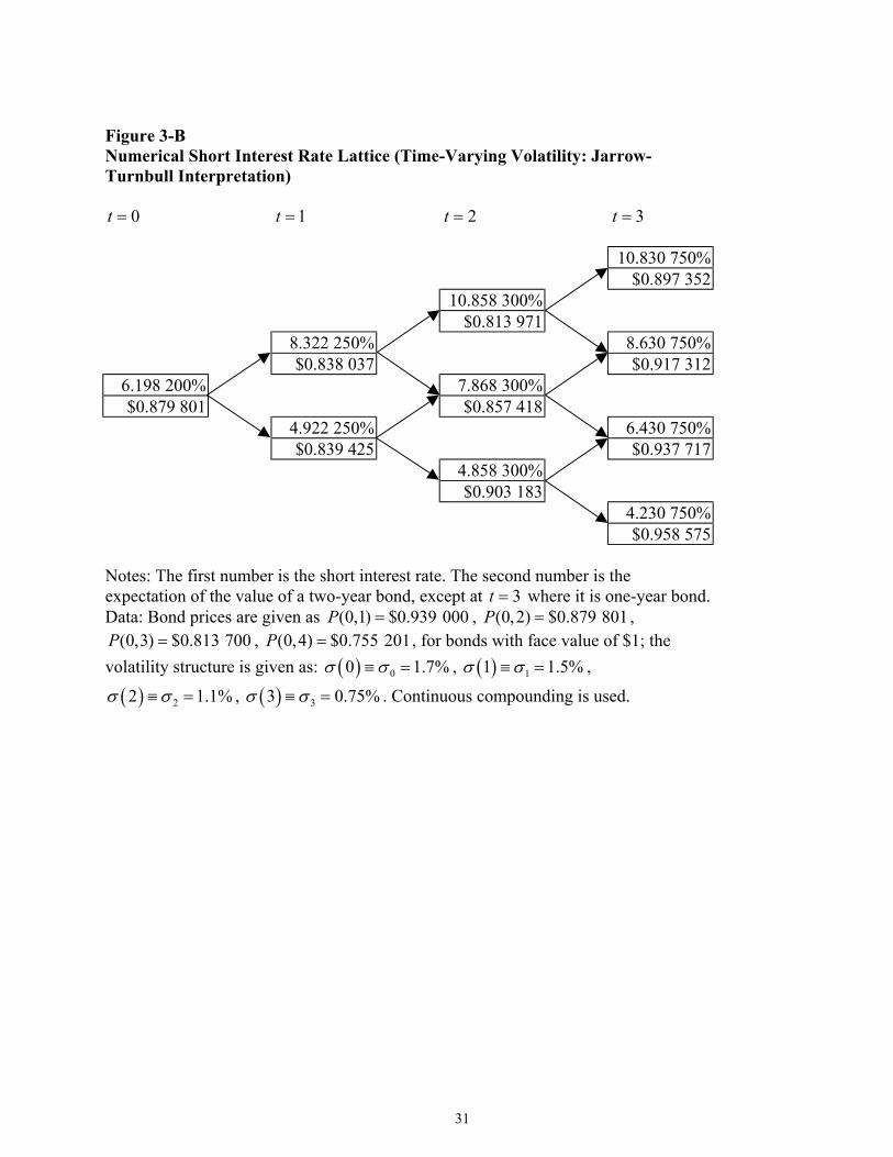
Figure 3-B Numerical Short Interest Rate Lattice (Time-Varying Volatility: Jarrow-Turnbull Interpretation)
0t = 1t = 2t = 3t =
10.830 750% $0.897 352 10.858 300% $0.813 971 8.322 250% 8.630 750% $0.838 037 $0.917 312
6.198 200% 7.868 300% $0.879 801 $0.857 418
4.922 250% 6.430 750% $0.839 425 $0.937 717 4.858 300% $0.903 183 4.230 750% $0.958 575
Notes: The first number is the short interest rate. The second number is the expectation of the value of a two-year bond, except at t where it is one-year bond. Data: Bond prices are given as , ,
, , for bonds with face value of $1; the volatility structure is given as: , ,
, . Continuous compounding is used.
3=(0,2P
( )1σ σ
(0,1) $0.939 000P =$0.755 201=
( ) 00 1.7%σ σ≡ =
0.75%
) $0.879 801=
1 1.5%≡ =(0,3) $0.813 700P =
( ) 22 1.1%σ σ≡ =
(0,4)P
( ) 33σ σ≡ =
31
32
Notes
( )0,P T 0=
1 2 31, 2, 3,T= = =
† We thank the anonymous reviewer and the editor Manuchehr Shahrokhi for their patience and invaluable comments and suggestions. Further, we thank the participants of the 2001 Global Finance Conference for their comments. * Douglas M. Brown Professor of Finance, Anderson School of Management, University of New Mexico, Albuquerque, NM 87131-1221. Tel: 505-277-5995, fax: 505-277-7108, e-mail: [email protected]. ** Associate Professor of Finance, Anderson School of Management, University of New Mexico, Albuquerque, NM 87131-1221. Tel: 505-277-0669, fax: 505-277-7108, e-mail: [email protected]. 1 Kijima and Nagayama (1994) may be considered to have done something similar in their development of what they call the shift function. Their results are derived in the continuous-time setting and then implemented for the Hull and White trinomial tree. Whether their results are generalizable and applicable in a wider context is unknown. Hull and White (1990a, 1990b) explore extensions of the Vasicek model that provide an exact fit to the initial term-structure of interest rates. When the speed of mean-reversion is set to zero, the Hull-White model reduces to the Ho-Lee model. Hull and White provide two implementations of their continuous-time model, viz., trinomial-tree building and explicit finite-difference method, based on a demonstration by Brennan and Schwartz (1978). In a series of subsequent articles, they expound upon the trinomial-tree method. While their model does provide elegant mathematical tractability to subsume earlier models as special cases of the Hull-White model, they do not provide an analytical model to obviate the need for a numerical trial-and-error method for computing the values on a trinomial lattice. Hull (2000) provides software-based help in building a trinomial-tree with up to ten steps. 2 This is a short-form notation for where the price is given at date t for maturity of T periods (years). T
can be designated as T T etc. The long-form notation will be useful in the later sections. 3 For example, we can illustrate that the equivalence with respect to the expected rate of return on the two-period bond from time 0 (zero) to time 1:
(1) (1)(0) (0) (1)
22 2
ln (0) or r r
r r rE e E e
r e or P E eP P
− −− −
= = =
0n =2n t=
( )( )2 r tσ ( )tσ
.
4 See Mood, Graybill and Boes (1974, p. 117) for a discussion of this result. 5 Boyle (1978) was the first one to point out this general result. 6 If the evolution can be depicted as a lattice, then the nth node means n up-moves. On the other hand, if the evolution is depicted as a tree, then the nth node is an ordinal rank, starting with at the bottom of the tree and ending with
at the top of the tree at date t. Depending upon the context, one must infer whether the nth node shows n up-moves or shows the ordinal rank. 7 Note the distinction between and . The former is the variance of the short rate, the latter is the specified volatility structure of the short rates. 8 Annotated spreadsheets for these examples are available from authors upon request. 9 Hull (2000) provides a discussion of time-varying volatility and provide an Excel-based pedagogy-oriented software handling a limited number of models and dates. He, however, does not comment on the example or implementation method provided by Jarrow and Turnbull.