the history of the cross section of returns

The History of the Cross Section of ReturnsSeptember 2017

Juhani Linnainmaa, USC and NBER

Michael R. Roberts, Wharton and NBER

Introduction

• Lots of anomalies

• 314 “factors” Harvey, Liu, and Zhu (2015)

• What is mechanism behind anomalies

• Unmodeled risk? Mispricing? Data-snooping?

• Empirical strategy

• Exploit comprehensive accounting data from 1926 to 2016

1. Pre-sample period (Jaffe et al ’89, Davis et al ‘00)

2. In-sample period

3. Post-sample period (Jagadeesh and Titman ’01, Schwert ’03,

McLean and Pontiff ‘16)

© Michael R Roberts 2

Key Findings

• 78% of anomalies “disappear” in pre- and post-periods

• Sharpe ratios, alphas, and information ratios all decrease; volatility and

covariation increase

• Including investment and profitability

• Sharpe ratio of 5-factor strategy ≈ Market Sharpe ratio (0.5) in pre-

• Choice of in-sample period critical to significance

• Small changes attenuate/eliminate many existing results

• 22% of anomalies survive

• Pre-sample: real investment, equity financing, distress, ROE/ROA

• Post-sample: Sales and earnings, total financing, distress, ROE/ROA


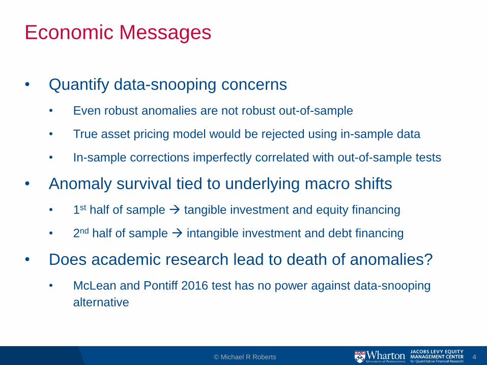
Economic Messages

• Quantify data-snooping concerns

• Even robust anomalies are not robust out-of-sample

• True asset pricing model would be rejected using in-sample data

• In-sample corrections imperfectly correlated with out-of-sample tests

• Anomaly survival tied to underlying macro shifts

• 1st half of sample tangible investment and equity financing

• 2nd half of sample intangible investment and debt financing

• Does academic research lead to death of anomalies?

• McLean and Pontiff 2016 test has no power against data-snooping

alternative


Data

• CRSP monthly returns 1926 to 2015

• Compustat 1962 to 2015 (+ some info back to 1947)

• Davis et al. ‘00 book value of equity 1926 to 1980

Moody's Industrial and Railroad Manuals 1918 to 1970

• Graham, Leary, and Roberts (2014, 2015)

• Limitations:

• No financials and utilities

• More aggregated than Compustat (e.g., no SG&A or R&D)

• Data quality

• Multiple checks and verifications (on top of checks in GLR)


Coverage


Illustrative Vehicle

• Profitability and investment factors

• Novy-Marx 2013, Fama and French 2015, Hou et al (2015)

• Profitability = OP/BE (FF 2015)

• Investment = Asset growth (FF, Hou et al.)

• Create HML-like factors for all anomalies

• E.g., Investment

• Portfolios held constant from July t to June t+1

• Avg return on two low portfolios and two high portfolios then difference

• Mitigate impact of small/micro firms


Monthly Factor Premiums by Era


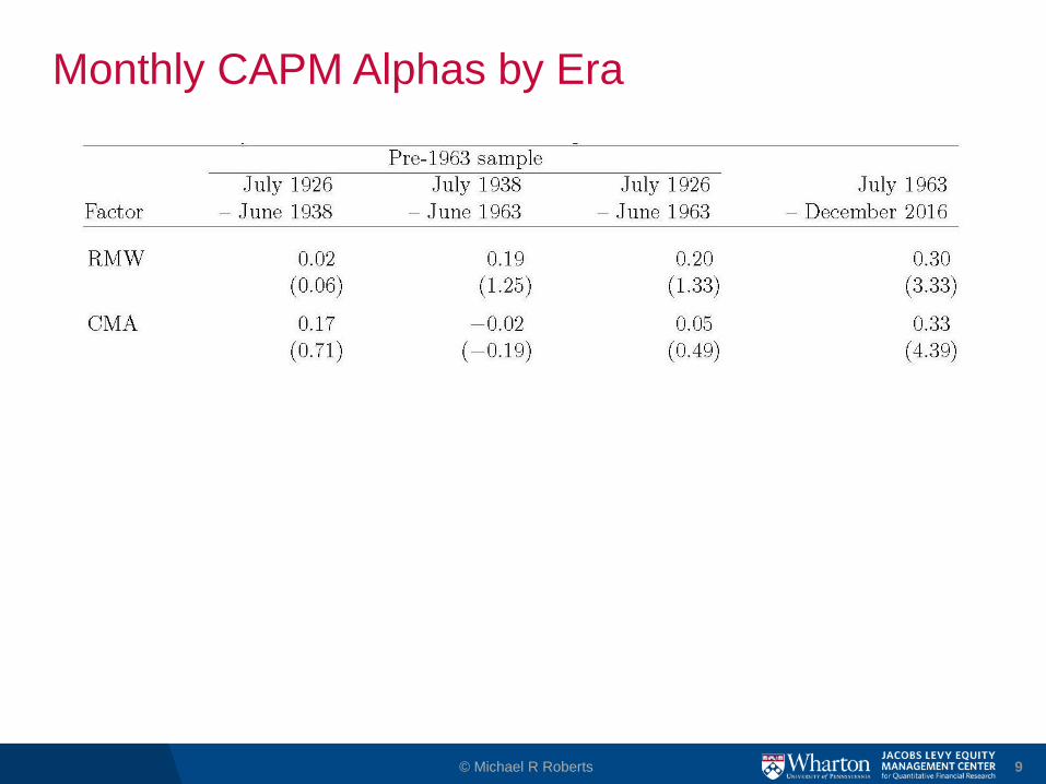
Monthly CAPM Alphas by Era


Monthly 3-Factor Alphas


Characteristic Distributions


The Rest of the Zoo


Statistically Significant Individual Anomalies

• In-sample

• Every anomaly CAPM or FF-3 alpha

• Pre-sample

• 8 average returns, 8 CAPM alphas, 16 FF-3 alphas

• Post-sample

• 1 average return, 10 CAPM alphas, 9 FF-3 alphas


Average Anomaly across Eras: Returns and Sharpe Ratios


• Average anomaly…

• Block bootstrap SEs

Average Anomaly across Eras: Alphas and Information Ratios


Identification Threats

• Unmodeled risk:

• Threat: Structural breaks

• Changes in risks that matter to investors, information costs

• Mispricing:

• Threat: Transient fads

• Learning:

• Investors learning and trade away anomalies


Are Start Dates “Judiciously” Chosen?


1963

Compustat Release

Gross Profitability 1963 - 2010

Return on Assets 1979 - 1993

Profit Margin 1984 - 2002

Cash Flow-to-Price 1968 - 1990

●

●

●

• All anomalies could have been measured as of 1963

• Was there a structural break around this time?

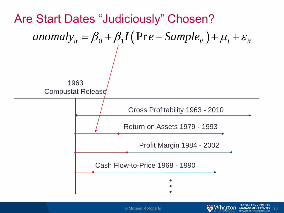
Are Start Dates “Judiciously” Chosen?


1963

Compustat Release

Gross Profitability 1963 - 2010

Return on Assets 1979 - 1993

Profit Margin 1984 - 2002

Cash Flow-to-Price 1968 - 1990

●

●

●

0 1 Prit it i itanomaly I e Sample

Structural Break Test



Average return drops by 50%




.

.

.Average return decline 40%-

80%




.

.

.

CAPM alpha decline

50%-75%




.

.

.

FF-3 alpha

decline

30%-90%

Correlation Structure of Returns

• How does an anomaly correlate with other anomalies

across eras?

• Motivated by Mclean and Pontiff (2016)


anomalyi,t

= a + b1Post

i,t+ b

2InSample Index

- i,t+ b

3PostSample Index

- i,t

+b4Post

i,t´ InSample Index

- i,t+ b

5Post

i,t´ PostSample Index

- i,t+ e

i,t

Correlation structure of returns: Post-sample


anomalyi,t

= a + b1Post

i,t+ b

2InSample Index

- i,t+ b

3PostSample Index

- i,t

+b4Post


- i,t+ b

5Post

i,t´ PostSample Index

- i,t+ e

i,t

Correlation structure of returns: Pre-sample


anomalyi,t

= a + b1Pr e

i,t+ b

2InSample Index

- i,t+ b

3Pr eSample Index

- i,t

+b4Pr e


- i,t+ b

5Pr e

i,t´ Pr eSample Index

- i,t+ e

i,t

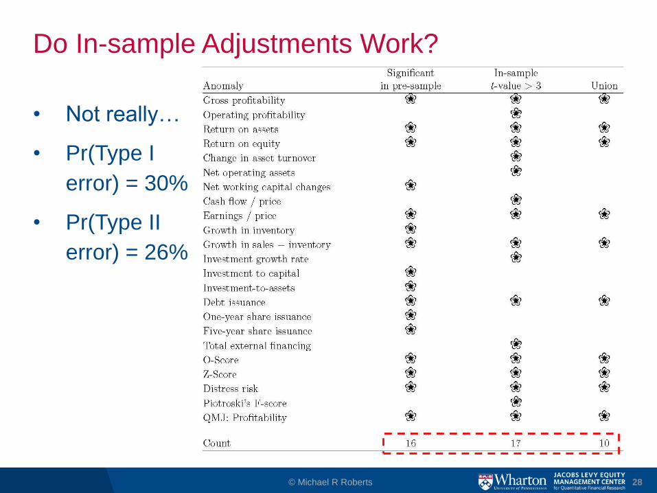
Do In-sample Adjustments Work?

• Not really…

• Pr(Type I

error) = 30%

• Pr(Type II

error) = 26%


Conclusions and Future Work

• Half-empty

• Data-snooping is severe

• Statistical adjustments have limitations

Out-of-sample testing (new data, holdout samples)

• Half-full

• Persistent violations of common AP models

• Appear correlated with economic fundamentals

• In-progress:

• What is the “right” model?

• How does this model tie into economic fundamentals?


the history of the cross section of returns

Documents