GGannett, Henry. Henry Gannett was an American geographer who is celebrated primarily for establishing new institutions within the federal government to col-lect and present information depicting aspects of the na-tion’s physical and human geographies. In doing this, he transformed the existing fragmentary approaches into a set of interrelated federal institutions that established a framework for the creation of integrated geographic information systems in the late twentieth century.

Gannett was born in Bath, Maine, 24 August 1846. He proved to be an academically gifted student, and af-ter graduating from high school in 1864 went to sea un-til entering Harvard’s Lawrence Scientifi c School in the fall of 1866. After graduation in 1869 he participated in a summer fi eld class led by J. D. Whitney, William Henry Brewer, and C. F. Hoffmann, all from the California Geological Survey, and Raphael Pumpelly, just returned from geological exploration in China. The class ranged from the Lake Superior mining region to Colorado. Gannett spent the subsequent academic year at Harvard obtaining a mining engineering degree, and upon gradu-ating in spring 1870 took his fi rst professional position as assistant to Joseph Winlock at the Harvard College Observatory. During the next two years, he compiled maps, prepared calculations to precisely measure the observatory’s longitude, and photographed the sun’s co-rona during the famous Mediterranean eclipse in Jerez, Spain.

In the spring of 1872 Gannett joined the U.S. Geo-logical and Geographical Survey of the Territories, led by F. V. Hayden, as its fi rst astronomer-topographer- geographer. He introduced scientifi c topographic map-ping to its existing geological and biological research programs. During seven years with the Hayden survey, Gannett led topographic mapping parties during sum-mer fi eld seasons in the Yellowstone National Park area,

Colorado, and Wyoming, and prepared reports and maps during winter offi ce seasons in Washington, D.C.

In 1879, when the federally sponsored scientifi c ex-peditions directed by Hayden, Clarence King, and John Wesley Powell were folded into the newly formed U.S. Geological Survey (USGS), the federal government was preparing to conduct its decennial census of population. At the request of the superintendent of the census, Fran-cis Amasa Walker, Gannett joined the tenth U.S. census (1880) in the newly created position of geographer. As the census’s fi rst geographer, he established geographic operations to collect information with a door-to-door enumeration of households; to compile that information; and then to present it in substantive reports with maps, charts, and text. These programs included the creation of enumeration districts that were based on the nation’s physical and human geographies for the fi rst time and dramatically improved the quality of census information. Gannett served as geographer–assistant director of three U.S. censuses and four censuses overseas—Cuba (twice), Puerto Rico, and the Philippines (North 1915, 10–11).

When the tenth U.S. census concluded in 1882, Gan-nett joined the USGS, headed by Powell. As its chief geographer, Gannett created the nation’s topographic mapping program. Once this program was established as an ongoing operation, he created several additional pro-grams that demonstrated the utility of topographically mapped geographic information for water issues and for the delineation and inventorying of timber stands. In so doing, he geographically defi ned the nation’s initial 110,000 square miles of national forests.

Gannett also chaired the federal government’s Board on Geographic Names for twenty years and served on numerous interagency commissions to coordinate fed-eral mapping and other scientifi c programs. In 1908–9, he directed the research program of President Theodore Roosevelt’s National Conservation Commission, which inventoried and projected future demand for the na-tion’s natural resources for the fi rst time.

During his long and productive career, Gannett devel-oped major new institutions not only within the federal government but in the private realm as well. He worked with others to found and manage the National Geo-

444 General Bathymetric Chart of the Oceans

graphic Society, Association of American Geographers, Cosmos Club, and Geological Society of Washington. He served as secretary of the 1904 Eighth International Geographical Congress (IGC), the fi rst to be conducted in the United States. In conjunction with the IGC, he formulated the standards that guided preparation of the International Map of the World (IMW) at the scale of 1:1,000,000. During his career, he published two hun-dred scientifi c and popular articles on human geogra-phy, cartography, and process geomorphology topics; edited journals; published academic textbooks; and served on a wide range of committees outside the federal government.

Many of Gannett’s programs continued remarkably intact up until the revolutionary transformation that resulted from the introduction of electronic computing at the close of the twentieth century. Elected a fellow of most of the major scientifi c organizations of his day, Gannett was additionally honored by foreign societies and governments; by Bowdoin College with an honor-ary doctorate; and most fi tting of all perhaps, by the naming of a physical feature for him. When the crest of Wyoming’s Wind River Range was measured to produce its fi rst topographic map sheets in 1906, the highest point, still unnamed, was designated Gannett Peak.

When Gannett died 5 November 1914, Washington, D.C., mourned the passing of this unassuming but re-markably productive individual with a memorial service at the National Geographic Society’s Hubbard Memo-rial Hall. Gannett was described then as the father of American mapmaking. Although a defi nitive biography of Gannett has yet to appear, several accounts provide useful introductions to his career (North 1915; Block 1984; Meyer 1999).

Donald C. Dahmann

See also: Board on Geographic Names (U.S.); Geographic Names: Applied Toponymy; U.S. Census Bureau; U.S. Geological Survey

Bibliography:Block, Robert H. 1984. “Henry Gannett, 1846–1914.” Geographers

Biobibliographical Studies 8:45–49.Meyer, William B. 1999. “Gannett, Henry.” In American National

Biography, 24 vols., ed. John A. Garraty and Mark C. Carnes, 8:675–76. New York: Oxford University Press.

North, S. N. D. 1915. Henry Gannett: President of the National Geo-graphic Society, 1910–1914. [Washington, D.C.]: National Geo-graphic Society.

Gazetteer. See Geographic Names: Gazetteer

General Bathymetric Chart of the Oceans (GEBCO).Bathymetric charts represent submarine relief. They are constructed with isobaths, which are contour lines connecting points of equal depth, and they often in-

clude shading between selected isobaths to indicate increasing depth. This type of thematic map became widespread only after the mid-nineteenth century due to technical, scientifi c, and economic factors: po-sitioning at sea, equipment, and methods for sounding all improved; marine sciences developed; and greater knowledge of seabed relief was needed to lay submarine cables.

Oceanographic expeditions continued to improve this knowledge during the last quarter of the nineteenth century. But simultaneously, nomenclature (the choice of names given to specifi c submerged features of relief) and terminology (terms describing forms of underwater relief) became anarchic. The Seventh International Geo-graphical Congress in Berlin (1899) addressed this is-sue (Carpine-Lancre 2005), and it adopted a resolution “nominat[ing] an international committee on the no-menclature of sub-oceanic relief, charged with instigat-ing the preparation and publication of a bathymetrical map of the oceans before the time of the meeting of the next Congress” (International Geographical Congress 1901, 1:314).

The Commission on Sub-Oceanic Nomenclature, composed of nine oceanographers and geographers, convened in Wiesbaden 15–16 April 1903, with Prince Albert I of Monaco as chair. For the design of the map they adopted most of the proposals submitted by French professor Julien Thoulet: sixteen sheets on the Merca-tor’s projection between 72°N and 72°S on the scale of 1:10,000,000; four sheets for each polar cap on the gnomonic projection; the use of the meter as the unit of measure; and Greenwich for the prime meridian (Thou-let 1904). The offer of Prince Albert I of Monaco to as-sume all expenses was gratefully adopted.

The twenty-four map sheets, the title sheet, and the as-sembly diagram for the Carte générale bathymétrique des océans were printed in Paris in 1905 (fi g. 280). Emman-uel de Margerie sternly criticized the errors and short-comings of this edition, which he felt was too speedily produced. Preparation of a new edition was entrusted to the newly constituted Prince’s Cabinet scientifi que, and a second commission that met in Monaco in 1910 de-cided to add terrestrial contour lines. The second edition was printed from 1912 to 1931. This long printing inter-val, partly due to World War I, made the chart obsolete before the last sheets were printed, and neither the Cabi-net scientifi que nor the Musée Océanographique de Mo-naco could afford the technical and fi nancial burden of a new edition insofar as the use of sonic and ultrasonic devices had greatly increased the available data.

The International Hydrographic Bureau (IHB) agreed to keep the General Bathymetric Chart of the Oceans (GEBCO) up to date. The fi rst step was an international inquiry about the usefulness of the chart and desired

Genetics and Cartography 445

improvements. Eight revised sheets were printed from 1935 to 1942. After World War II, in spite of the help given by the French Institut géographique national, the IHB was unable to bring the third edition to a successful conclusion (the last three sheets appeared in 1968, and three sheets were never printed). A fourth edition was started in 1958, its preparation shared between eighteen hydrographic services, however only six sheets were printed (up to 1971).

Additional problems needed to be solved. During the Cold War, bathymetric data acquired immense strategic value for submarine navigation. Most of the new infor-mation was classifi ed, leading the Lamont Geological Observatory to create a different type of bathymetric chart: the physiographic diagram. However, marine sci-entists felt more than ever that GEBCO was still neces-sary, but that it must be produced with greater coopera-tion of scientists with cartographers for interpretation of the data. The international organizations related to oceanography, including the International Association of Physical Oceanography, the Scientifi c Committee on Oceanic Research, and the Intergovernmental Oceano-graphic Commission of UNESCO (United Nations Edu-cational, Scientifi c and Cultural Organization), brought increasing attention to the endeavor, and their efforts were successful. The fi fth edition was published in 1982 by the Canadian Hydrographic Service, with the eigh-teen sheets receiving different numbering and boundary limits than previous editions (fi g. 281).

The permanent problem of updating the chart led to the digitization of the data by the British Oceanographic Data Centre. A digital atlas was published on CD-ROM in 1994 and revised in 1997. A centenary edition was prepared and distributed on the occasion of the meeting held in Monaco in 2003 (British Oceanographic Data Centre 2003; Scott 2003). The latest development is the 1-minute Global Bathymetric Grid (2006).

Jacqueline Carpine-Lancre

See also: Digital Worldwide Mapping Projects; Geographic Names: (1) Applied Toponymy, (2) Gazetteer; International Hydrographic Organization (Monaco); Law of the Sea; Marine Chart; Marine Charting

Bibliography:British Oceanographic Data Centre. 2003. GEBCO Digital Atlas,

Centenary Edition of the IHO/IOC General Bathymetric Chart of the Oceans. CD-ROM, 2 discs. Swindon: Natural Environment Re-search Council.

Carpine-Lancre, Jacqueline. 2005. “Une entreprise majeure de la car-tographie océanographique: La Carte générale bathymétrique des océans.” Le Monde des Cartes 184:67–89.

International Geographical Congress. 1901. Verhandlungen des Sie-benten Internationalen Geographen-Kongresses, Berlin, 1899. 2 vols. Berlin: W. H. Kühl.

Scott, Desmond, ed. 2003. The History of GEBCO, 1903–2003: The 100-Year Story of the General Bathymetric Chart of the Oceans. Lemmer, Netherlands: GITC.

Thoulet, Julien. 1904. “Carte bathymétrique générale de l’Océan.” Bulletin du Musée océanographique de Monaco 21:1–27.

Genetics and Cartography. Perhaps the fi rst attempt to represent genetic data on a geographic map can be attributed to J. B. S. Haldane, considered one of the founders of population genetics. This branch of genetics focuses on gene and DNA variants, in particular on their frequency, distribution, and change under the infl uence of the four evolutionary forces: natural selection, genetic drift, mutation, and gene fl ow. To interpret the results, population geneticists take into account population sub-divisions and population differences in space, termed “ge-netic structures” because, in genetics, “cartography” re-fers exclusively to the mapping of genes on chromosomes.

In 1940 Haldane plotted the blood-group frequen-cies of European peoples as mathematically computed contour maps. Following in the steps of physical an-thropologists, he sought to infer the past of European populations, up to Neolithic times, from present-day genetic variability. For almost forty years after Haldane, the only genetic markers offering a satisfactory world-wide geographic coverage of human populations were still constituted by blood phenotypes, as demonstrated by the research (through 1976) of A. E. Mourant and his colleagues, who similarly displayed their results as contour maps with isolines threaded manually—“by eye”—rather than estimated mathematically. The main preoccupation at the time was the identifi cation of new markers and DNA variants as well as their localization on chromosomes. This is why the effort of population geneticists to represent their data geographically was minimal.

The ability to use DNA variation to reconstruct the demographic history of populations increased through the 1970s and exploded in the last decade of the twen-tieth century with the advent of PCR (polymerase chain reaction), a method to replicate DNA sequences. New markers became available and human populations were typed intensively. While the use of several markers pro-moted more reliable studies by minimizing stochastic er-rors, a new approach to geographic mapping of the re-sults was needed because thematic maps describing the variability of a single marker were no longer effi cient. A solution suggested by Alberto Piazza involved using principal components analysis (PCA) to reduce a large number of markers to the fi rst components (often the fi rst, second, and third) and plotting each of them on a separate three-dimensional map. On each map individ-ual samples were represented by (x, y, z) points, where x and y were the longitude and latitude coordinates and z was the component score. Adopted in 1994 in a refer-ence book about the history and geography of human

446 Genetics and Cartography

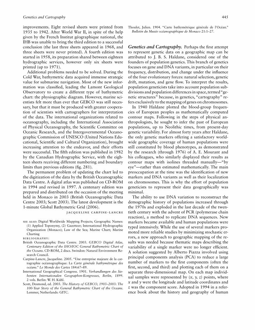
Fig. 280. DETAIL OF THE AZORES, CARTE GÉNÉRALE BATHYMÉTRIQUE DES OCÉANS, FIRST EDITION, 1905. Paris: Impr. Erhard, twenty-four sheets at a scale of 1:10,000,000. This part of sheet A1 shows an area extensively studied by Prince Albert I of Monaco, during his oceanographic cruises.

Size of the detail: ca. 20 × 21 cm. Image courtesy of the Amer-ican Geographical Society Library, University of Wisconsin–Milwaukee Libraries.

genetic variability (fi g. 282), this technique caught the attention of scholars outside the discipline (notably ar-chaeologists and historical linguists) as well as a broader public.

However intriguing, these maps conveyed a false sense of precision insofar as the interpolation process used to fi t contour lines to point data strongly infl uenced the mapped pattern. To provide more reliable maps of ge-

netic differences, Guido Barbujani and Robert R. Sokal (1990) adopted the Wombling procedure (Womble 1951) to identify the zones of abrupt genetic change. Later, Barbujani et al. (1996) introduced in genetics the maximum difference algorithm developed by Mark Monmonier (1973). This method proved well suited for identifying, without resort to interpolation, those sam-ples highly different from their neighbors.

Genetics and Cartography 447

Boundary methods epitomize the geneticist’s interest in the difference between populations rather than in their ho-mogeneity. This is understandable insofar as only 15 per-cent of the variance of the human genome is explained by differences between groups of populations, in contrast to individual differences within a population, which account for 85 percent of the total variance—the reason why the scientifi c defi nition of race does not apply to humans.

In the 1980s, work by population geneticists pro-moted the study of the geographical distribution of genealogical lineages, termed “phylogeography” (Avise 1998; Hewitt 2001). Such studies proved to be effective in reconstructing refugia (areas that fostered relict spe-cies by escaping wider ecological changes), postglacial colonization routes, and the speciation processes of dif-ferent organisms. These studies also helped geneticists

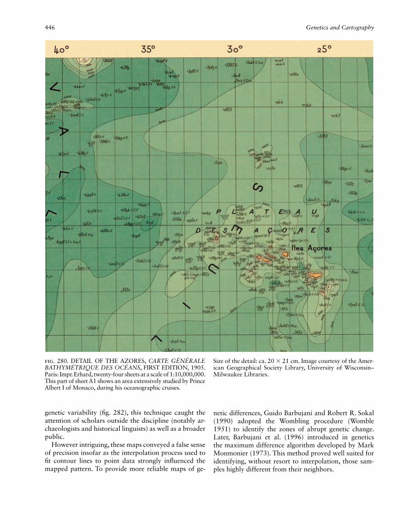
Fig. 281. DETAIL OF THE AZORES, GENERAL BATHY-METRIC CHART OF THE OCEANS/CARTE GÉNÉRALE BATHYMÉTRIQUE DES OCÉANS, FIFTH EDITION, 1982. Canadian Hydrographic Service, eighteen sheets, at various sizes and scales. This part of sheet 5-08 illustrates the changes between the fi rst and the fi fth editions of the chart. Ottawa: Canadian Government Publishing Centre.

Size of the detail: ca. 19.9 × 21.6 cm. Reproduced with the permission of the Canadian Hydrographic Service, Ottawa. In a standard disclaimer, the publisher advises that the chart is “not to be used for navigation.”

448 Geocoding

defi ne appropriate policies for preserving endangered species (or populations), avoiding excessive levels of consanguinity in living stocks, and reintroducing ani-mals with a genetic makeup similar to that of an extinct or displaced species. Such tasks required a straightfor-ward and effective evaluation of the habitat based on a refi ned level of geographic detail and on the use of geographic information systems.

Although geographic cartography used in genetics in the latter half of the twentieth century might appear simplistic, new challenges seem likely as a result of ef-forts by Gustave Malécot (1948) and other theorists to mathematically model the relations existing between the genetic distance between pairs of populations and the corresponding geographic distance. An appropriate rep-resentation of this model may inspire the next step in the geographic portrayal of genetic differences.

Franz Manni

See also: Biogeography and Cartography; Ethnographic Map; Lin-guistic Map; Statistics and Cartography

Bibliography:Avise, John C. 1998. “The History and Purview of Phylogeography: A

Personal Refl ection.” Molecular Ecology 7:371–79.Barbujani, Guido, and Robert R. Sokal. 1990. “Zones of Sharp Ge-

netic Change in Europe Are also Linguistic Boundaries.” Proceed-ings of the National Academy of Sciences of the United States of America 87:1816–19.

Barbujani, Guido, et al. 1996. “Mitochondrial DNA Sequence Varia-tion across Linguistic and Geographic Boundaries in Italy.” Human Biology 68:201–15.

Cavalli-Sforza, L. L., Paolo Menozzi, and Alberto Piazza. 1994. The History and Geography of Human Genes. Princeton: Princeton University Press.

Haldane, J. B. S. 1940. “The Blood-Group Frequencies of European Peoples, and Racial Origins.” Human Biology 12:457–80.

Hewitt, Godfrey M. 2001. “Speciation, Hybrid Zones and Phylogeog-raphy—Or Seeing Genes in Space and Time.” Molecular Ecology 10:537–49.

Malécot, Gustave. 1948. Les mathématiques de l’hérédité. Paris: Masson.

Monmonier, Mark. 1973. “Maximum-Difference Barriers: An Alter-native Numerical Regionalization Method.” Geographical Analysis 5:245–61.

Mourant, A. E., Ada C. Kopec, and Kazimiera Domaniewska-Sobczak. 1976. The Distribution of the Human Blood Groups, and Other Polymorphisms. 2d ed. London: Oxford University Press.

Womble, William H. 1951. “Differential Systematics.” Science, n.s. 114:315–22.

Geocoding. In the 1960s and 1970s the term “geo-coding” referred to a broad array of activities associ-ated with systems of referencing data spatially (Dueker 1974). Geocoding was a central element of methods for computer processing of geographic data. Waldo R. To-bler (1972) defi ned geocoding broadly as place naming, with two types of place-names. The fi rst are nominal or ordinal names or codes that require a map to infer lo-cation. The second are coordinate-based, which make geographical relationships explicit. Early geocoding sys-tems dealt with the fi rst type of place-names, process-ing codes for places that were not geometrically defi ned (Shumacker 1972). Over time, geocoding systems moved from the fi rst type of place-names to a more explicit en-coding of spatial location and geographical relationships. Currently, geocoding is thought of more strictly as the

Fig. 282. SYNTHETIC MAP OF THE AMERICAS USING THE FIRST PRINCIPAL COMPONENT. Example of Alberto Piazza’s strategy for mapping separately principal components (PCs) extracted from a multivariate set of marker data. This synthetic map displays the fi rst of the seven PCs that were computed. It accounts for the variation of seventy-two genes and explains 32.6 percent of the total variance. The map shows a north-south gradient in North and Central America with the greatest slope in Canada, thus emphasizing the dis-tinction between the Eskimos + Na-Dene group and Amerind populations closer to Eskimos on the one side, and the rest of America on the other. In South America there is differentiation between east and west. For easy visual recognition, Piazza used eight classes of PC values, but his choice of the increasing or decreasing density of shading is totally arbitrary; it could be reversed without any loss of information. Intermediate classes are close to the average, whereas extreme classes indicate pop-ulations that globally differ most from each other for the par-ticular PC under study. Populations and regions with similar shading do not need to be similar, for they may be very differ-ent for another PC. In such synthetic maps, Piazza preferred not to display the location of samples.Size of the original: 9.5 × 8.3 cm. From Cavalli-Sforza, Menozzi, and Piazza 1994, 338 (fi g. 6.13.1). © 1994 Princeton University Press. Reprinted by permission of Princeton University Press.

Geocoding 449

process of assigning geographic coordinates expressed in latitude-longitude or x, y form to map features and associated data records referenced by a street address. Geocoding has been closely tied to geographic infor-mation systems (GIS) and is now commonly thought of as the process of fi nding the location of an address with a GIS (Arctur and Zeiler 2004). Street addresses are the most commonly used means by which users can enter their location of interest to GIS. These addresses are geocoded to geographic coordinates or geographic unit codes employed in GIS. With the advent of Global Positioning System (GPS) technology in the 1980s, re-verse geocoding was developed for the assignment of GPS-derived latitude and longitude values to streets and intersections, as well as to nearby points of interest such as an address of a business.

Geocoding relies on directories or databases to con-vert addresses or place-names to geographic area codes or coordinates. This requires complete street address in-formation and an accurate geocoding database of place codes and coordinates. Early geocoding efforts in the United States focused on standardizing place codes used by various state and federal agencies. Standardization of state, county, and city codes was needed to collect shar-able data. However, efforts to standardize geocoding be-low the city and county level fl oundered due to the lack of a common small geographic area, such as a city block, that served a broad community of users (Werner 1974, 312). National-level geocoding in the United States had to await two developments: extension of urban-style addresses to rural areas to support emergency dispatch and the development of a nationwide geographic base fi le, TIGER Line (Topologically Integrated Geographic Encoding and Referencing), by the U.S. Bureau of the Census, which was fi rst used in 1990, replacing Dual Independent Map Encoding (DIME), which was limited to metropolitan areas.

Urban area geocoding efforts emerged independently in several locations but developed largely in conjunction with planning and implementation of the 1970 U.S. Cen-sus of Population and Housing (Dueker 1974). The U.S. Bureau of the Census developed address coding guides (ACG) for metropolitan areas to automate enumeration using mail-out and mail-back questionnaires. The ACG consisted of a table of ranges of street addresses within each census block (Fay 1966). Figure 283 illustrates the dual encoding of a line network consisting of street seg-ments with adjacent blocks. Table 14 illustrates the con-ceptual format of the ACG that assigns a street address to census block, tract, and county codes for subsequent tabulation for streets in fi gure 283. Field testing showed compilation of an ACG was error prone since it was easy to transpose right and left codes and diffi cult to detect these errors. Nevertheless, the computerized data access

and use procedures developed for the 1970 census were responsible for creating the current demographic analy-sis industry (Cooke 1998).

To remedy defi ciencies of the ACG the Census Bureau developed the DIME mapping process that was based on applying mathematics of graph theory and topology to the urban street system (Corbett 1979). When com-bined with the address coding guide, it was called ACG/DIME. By 1980, ACG/DIME had been renamed Geo-graphic Base File DIME (GBF/DIME).

The 1966 New Haven Census Use Study provided a test bed for DIME fi le design and implementation (Cooke and Maxfi eld 1967). The street system was en-coded as a graph with nodes representing intersections (and bends in roads and ends of dead-end streets), and lines representing street segments (and railroads, politi-cal boundaries, and water features) that make up areas representing census blocks. The mathematical dual is a boundary network consisting of blocks with bounding streets. Chaining boundary streets around blocks is done to verify that streets are encoded correctly. This editing ensured the integrity of the GBF/DIME.

Geocoding involves a spatial lookup of an address against a geographic database that spatially encloses any possible address and whose address style is of the same type as the addresses being geocoded. The spa-

1617 20 19

1514 12

6710

9

54 1 2

Block no.

11

Tract no.

Tract no.

Oak St.

Elm St.

Ash St.

N. 5th A

ve.

N. 6th A

ve.

N. 7th A

ve.

5450

5533

5621

5622

5532

5451

5623

5531

Node

no.

ShapePoint

109 110

109 110

598599601

602

501502

1298 1299

1202 1201

699698

D

C

C = Parcel CentroidD = Estimated Location

at 635 Elm St.

Fig. 283. DUAL ENCODING OF STREET SEGMENTS AND BLOCKS.

450 Geocoding

tial look-up process depends on effi cient parsing of addresses to standardize abbreviations and to separate component parts—number, street prefi x, street name, and street type—as well as on effi cient spatial indexing of address ranges by state, city, and/or ZIP code. The geocoding process then searches for matches between the input address and the geographic database. The pro-cedure may fi nd a number of possible matches; users may be asked to choose from a list of candidates, or the procedure may assign probabilities for selection of the correct street segment when doing bulk geocoding.

The U.S. Bureau of the Census (1971) led in the de-velopment of ADMATCH geocoding software as the address matching system for DIME fi les used in the 1970 Census. ADMATCH operated by linking a data fi le containing street addresses or address ranges and a geographic reference fi le containing street addresses and corresponding geocodes. A matcher program analyzed the street addresses in the data fi le according to syntax and keywords specifi ed by the user and created a stan-dard version of each address called a match key. Each match key was then compared with the geographic ref-erence records with the same street name and the best match was selected according to a weighting scheme de-fi ned by the user.

The GBF/DIME fi le system was followed by the devel-opment of TIGER, the seamless nationwide digital map fi le system. TIGER was implemented by U.S. Census Bureau geographer Robert W. Marx and his team for the 1990 Census (Cooke 1998, 54–55; Marx 1986). The main differences between DIME and TIGER fi les were better cartography and extended coverage from metro-politan areas to nationwide in the TIGER system. Leg-acy TIGER Line fi les and the redesigned master address fi les (MAF/TIGER) have become the database basis for modern address geocoding systems (Galdi 2005).

Vendors commercializing geocoding for business GIS use have played an important role in extending geocod-

ing content and performance. In the 1970s Urban Data Processing Inc. used street address matching software with Census ACG/DIME fi les to provide geocoding ser-vices for 85 of the 100 largest banks in the United States. This was the fi rst major commercialization of geocod-ing. Both Geographic Data Technology (GDT) and Etak purchased Census GBF/DIME and TIGER fi les in the 1980s, improved their accuracy and currentness, and sold the improved databases and geographic services both to businesses and a growing vehicle navigation market. Etak and GDT wrote and commercialized batch and interactive address matching programs for geocod-ing with their databases.

By century’s end geocoding was commonplace. Busi-ness information systems often start by asking for a person’s ZIP code, and the system responds with ad-dresses of their stores within the ZIP code or in nearby ZIP codes (Wombold and Ting 2006). This capability is based on a database of adjacent or nearby ZIP codes. This is a coarse geocoding based on geographic areas rather than coordinates. More precise geocoding con-verts a unique street address to a unique coordinate lo-cation, which enables business information systems to distance order their stores from the street address, using either straight line or on-street distance. Current data-base products provide addresses accurate to individual buildings. Addresses are represented as discrete points rather than approximations interpolated from address ranges for street segments.

Vehicle navigation systems, using Navteq street cen-terline databases and Internet map services like Map-Quest, calculate routes from geocoded origins and desti-nations and provide driving instructions and a map with highlighted street route segments. Using Google Maps to zoom to a specifi c location below the city level in-volves geocoding an address from an underlying Navteq street centerline database. Then one can zoom in or out and drape imagery on the map.

Table 14. Address coding guide: the table look-up approach

Odd/evenLow address

High address

Street prefi x

Street name

Street type

Street suffi x

Block number

Tract number

E 502 598 Ash St 6 109

O 501 599 Ash St 5 109

E 502 598 Elm St 15 109

O 501 599 Elm St 6 109

E 1202 1298 N 5 Av 7 109

O 1201 1299 N 5 Av 6 109

E 1202 1298 N 6 Av 6 109

O 1201 1299 N 6 Av 10 110

Geocoding 451

Assigning a geocode involves conversion of place-names and street addresses that are familiar to position-ally accurate coordinates that can be used for computing distances and assignment to areas by means of a point-in-polygon routine. Table 15 illustrates the positional accuracy of various geocoding methods.

The more commonly known geographic place-names for cities, counties, and states do not yield very precise locations. Street addresses can yield greater positional accuracy if investments are made in look-up tables based on accurate positions of streets, parcels, or build-ings. While geocoding in the United States relies heavily on street address conversion, other countries with more centralized land records rely on land and property data to construct street addresses used in land parcel look-up tables to improve geocoding accuracy (Morad 2002).

Some geocoding systems rely on look-up tables to directly relate addresses to school attendance areas, emergency service zones, and other service areas. This is not recommended, however, as a change in service area boundaries requires extensive and error-prone updating of the look-up tables. Representation of service areas as polygons and addresses as coordinate points leads to fewer geocoding errors.

The need for positional accuracy depends on the ap-plication. For example, environmental health applica-tions may need to geocode the locations of patient homes relative to toxic waste plumes. Geocoding accuracy of plumes, whether aerial, surface, or subsurface, is also an issue. Similarly, accurate assignment of welfare cases to statistical areas is needed to assess causes of poverty.

The six character postal codes in Canada fully imple-mented in 1974, alphanumeric post codes in Britain in-troduced over a fi fteen-year period from 1959 to 1974, and fi ve-digit ZIP codes begun in the United States in 1963 are useful because people know them and they are easy to relate to a point location. But they do not relate to unambiguous areas. Postal codes can denote a specifi c single address or range of addresses, which can corre-

spond to an entire small town, a signifi cant part of a medium-sized town, a single side of a city block in larger cities, a single large building or a portion of a very large one, a single (large) institution such as a university or a hospital, a business that receives large volumes of mail on a regular basis, postal facilities, or a rural route. A postal code can be wholly contained in another. In 1970, the U.S. Bureau of the Census provided approximated ZIP code tabulations (three-digit ZIP codes outside of Standard Metropolitan Statistical Areas [SMSAs] and fi ve-digit ZIP codes inside SMSAs), for 1980 as a special tabulation, in 1990 based on an equivalency fi le relating commercial census blocks to ZIP codes, and in 2000 and 2010 by ZIP Code Tabulation Areas (ZCTA) based on groupings of census blocks.

The development of reference data that were strength-ened by applying principles of topology to the encoding of map information advanced rapidly during the lat-ter half of the twentieth century, as computing power increased. Until the advent of robust GIS software in the 1980s, homegrown software tools were developed for aggregating discrete data to small area data for map display and analysis. The process of assigning a small area code to data with a street address as the location identifi er became known as geocoding. Building refer-ence databases for geocoding was a major issue from the mid-1960s to the late 1980s when TIGER became stable and GIS software tools to use it became widely available. The U.S. Bureau of the Census was largely responsible for standardizing and developing reference materials needed for geocoding in the United States. Al-though their motive was to convert to a mail-out, mail-back decennial census of population and housing, the reference materials have served many uses and have be-come building blocks for many GIS databases through-out the world, as TIGER-like databases have developed elsewhere. Other countries developed similar databases, though the lack of systematic street addressing posed a major problem, especially in developing countries.

Table 15. Geocoding accuracy and method

Positional Accuracy (low to high) Geocoding Method Example

+/– 10,000 m County name to centroid table Relate vital statistics to population data

1000 m Street address to census tract table Relate individual health data to areas of high poverty

1000 m ZIP code to centroid fi le Find nearby businesses

100 m Interpolate addresses along street segments Find approximate locations

10 m Street address to land parcel table Find parcel boundary/centroid

10 m Street address to building footprint table Find building boundary/centroid

1 m GPS Find precise location directly

452 Geodesy

Geocoding has become commonplace as it is the fi rst step in converting street addresses to geographic coordi-nates for a wide range of GIS applications. Meanwhile, GPS is emerging as a means of direct entry of locations into a GIS and may reduce the need for geocoding.

Kenneth J. Dueker

See also: Canada Geographic Information System; Census Map-ping; Electronic Cartography: Data Structures and the Storage and Retrieval of Spatial Data; Geographic Information System (GIS): (1) Computational Geography as a New Modality, (2) GIS as a Tool for Map Analysis and Spatial Modeling; Software: Geographic In-formation System (GIS) Software

Bibliography:Arctur, David, and Michael Zeiler. 2004. Designing Geodatabases:

Case Studies in GIS Data Modeling. Redlands: ESRI.Cooke, Donald F. 1998. “Topology and TIGER: The Census Bureau’s

Contribution.” In The History of Geographic Information Systems: Perspectives from the Pioneers, ed. Timothy W. Foresman, 47–57. Upper Saddle River: Prentice Hall PTR.

Cooke, Donald F., and William H. Maxfi eld. 1967. “The Development of a Geographic Base File and Its Uses for Mapping.” In Urban and Regional Information Systems for Social Programs: Papers from the Fifth Annual Conference of the Urban and Regional Information System Association, ed. John E. Rickert, 207–18. [Kent: Center for Urban Regionalism, Kent State University.]

Corbett, James P. 1979. Topological Principles in Cartography. [Washington, D.C.]: U.S. Department of Commerce, Bureau of the Census.

Dueker, Kenneth J. 1974. “Urban Geocoding.” Annals of the Associa-tion of American Geographers 64:318–25.

Fay, William T. 1966. “The Geography of the 1970 Census: A Coop-erative Effort.” Planning: Selected Papers from the ASPO National Planning Committee, 99–106.

Galdi, David. 2005. Spatial Data Storage and Topology in the Rede-signed MAF/TIGER System. Washington D.C.: U.S. Bureau of the Census, Geography Division. Online publication.

Marx, Robert W. 1986. “The TIGER System: Automating the Geo-graphic Structure of the United States Census.” Government Publi-cations Review 13:181–201.

Morad, M. 2002. “British Standard 7666 as a Framework for Geocod-ing Land and Property Information [in] the UK.” Computers, Envi-ronment and Urban Systems 26:483–92.

Shumacker, Betsy. 1972. “Geo-coding and Geo-defi nition.” In Proceed-ings: The National Geo-coding Conference, III.28–III.30. Washing-ton, D.C.: Department of Transportation.

Tobler, Waldo R. 1972. “Geo-coding Theory.” In Proceedings: The National Geo-coding Conference, IV.1–IV.2. Washington, D.C.: De-partment of Transportation.

U.S. Bureau of the Census. 1971. Census Use Study: Geocoding with ADMATCH, a Los Angeles Experience. Washington, D.C.: U.S. De-partment of Commerce.

Werner, P. A. 1974. “National Geocoding.” Annals of the Association of American Geographers 64:310–17.

Wombold, Lynn, and Edmond Ting. 2006. “A Break from the Past: Understanding ESRI’s 2006 Demographic Updates.” ArcUser 9, no. 4:8–11.

Geodesy.Geodetic TriangulationGeodetic TrilaterationGravimetric Surveys

Satellite GeodesyGeodetic ComputationsGeodesy and Military Planning

As the science of measuring the size and shape of the earth, geodesy includes a number of technologies and institutional practices with distinct histories. The order of articles in this composite refl ects a progression from older to newer forms of measurement as well as the emer-gence of a prominent military role during the Cold War. A separate composite entry, “Geodetic Surveying,” ad-dresses the application of geodesy within major regions.

Geodetic Triangulation. Triangulation is a method of terrestrial surveying in which points on the ground (of-ten called stations) whose coordinates are to be deter-mined are the vertices of triangles. The vertices are per-manently marked or monumented points so they can be recovered for future use. Individual triangles are joined together to form chains or networks (fi g. 284). When triangulation must take into account the fi gure and size of the earth because a large land area is encompassed, it is called geodetic triangulation. Developed in the eighteenth century, the principles of geodetic triangula-tion were important throughout the twentieth century in framing topographic and other forms of large-scale mapping.

In geodetic triangulation, the horizontal angles at each point in each of the triangles are measured with precise optical instruments called theodolites. Usually, all of the angles in every triangle are measured to provide redun-dancy as well as data for estimating the precision of the measurements. A surveyor who has measured the angles and knows the length of one side can use trigonometry

B

A

С

Fig. 284. SIMPLE TRIANGULATION NET. The known data are: length of baseline AB, latitude and longitude of points A and B, and azimuth of line AB. The measured data are: the angles to new control points. Computed data are: latitude and longitude of point C and other new points, length and azimuth of line AC, and length and azimuth of all other lines. Burkard’s Geodesy for the Layman was a useful introduction to geodesy provided gratis by the Defense Mapping Agency.After Burkard 1959, 26 (fi g. 14).

Geodesy 453

to compute the lengths of the remaining sides of any triangle. To compute the coordinates (latitudes and lon-gitudes) of the network points, the surveyor must know the scale of the network, its orientation, and the coor-dinates of a starting point. Scale is provided either by measuring one side of one of the triangles (called a base line) or by calculating the intervening distance from the coordinates of two of the network points. Orientation is provided either by measuring the astronomic azi-muth along one of the sides of one of the triangles or by knowing the coordinates of two of the network points. In either case, the coordinates of at least one point must be known.

Because the horizontal angles are measured optically, the points forming a triangle must be intervisible. This requirement has limited the use of geodetic triangulation, particularly for projects in comparatively fl at regions. Unless the area has substantial topographic relief so that stations are readily intervisible, towers must be erected to raise the theodolites, targets, and personnel to obtain a clear line of sight. The expense of erecting towers and the associated liability of the personnel working on them is one of the reasons why geodetic triangulation was usu-ally undertaken by national mapping organizations or their counterparts at the state or provincial level. Also, to minimize the effect of lateral refraction on the line of sight, the horizontal angles in the more accurate trian-gulation surveys have typically been measured at night, when the atmosphere near the ground is most stable.

Prior to the development of electronic distance mea-suring (EDM) instruments and the use of satellite ge-odesy, geodetic triangulation was the most accurate method for determining the latitude and longitude of a station. Geodetic triangulation stations are classifi ed by their estimated accuracy between pairs of interconnected stations and are assigned an order and in some cases a suborder or class. The most accurate geodetic triangula-tion is classifi ed as fi rst-order, defi ned as having an er-ror no greater than 1 part in 100,000 for the distance between the station and its directly connected neighbor. Second-order class I and second-order class II surveys must have accuracies of 1 part in 50,000 and 20,000, respectively, while the error in a third-order survey may not exceed 1 part in 10,000. Each order and class has other specifi cations, which might include the intended or permissible uses of coordinates, the geometry of the network, the accuracy of instrumentation used, and the number of repeat measurements required.

The computation of geodetic triangulation data gen-erates horizontal control data that are expressed as a geodetic latitude and longitude for each station in the network. Horizontal control data provide the scale and orientation for all types of accurate charting and map-ping projects. They also provide the means for fi tting

together local, regional, state, and national mapping projects. In addition to its use for mapping and chart-ing, these data provide the means for locating national, state, and county boundaries; confi rming and increasing the accuracy of local and city surveys; and assisting in the perpetuation of points (including the preservation or restoration of monuments) established by such sur-veys. They support military defense mapping projects and provide data for computing accurate directions and distances for long-range positioning. Geodetic triangu-lation data have been utilized in scientifi c investigations such as measuring seismic shifts and other earth move-ment and determining the size and shape of the earth. Toward the end of the twentieth century, direct mea-surement of angles became less important in geophysi-cal research insofar as EDM instruments allowed direct measurement of distances in a triangulation system and global positioning systems provided accurate estimates of coordinates and elevations, eliminating the need for a network in many instances.

Edward J. McKay

See also: Figure of the Earth; Photogrammetric Mapping: Geodesy and Photogrammetric Mapping; Property Mapping Practices

Bibliography:Burkard, Richard K. 1959. Geodesy for the Layman. St. Louis: Aero-

nautical Chart and Information Center.Gossett, F. R. 1959. Manual of Geodetic Triangulation. Rev. ed. Wash-

ington, D.C.: Government Printing Offi ce.National Geodetic Survey (U.S.). 1986. Geodetic Glossary. Rock-

ville: National Oceanic and Atmospheric Administration, National Ocean Service.

Geodetic Trilateration. The National Geodetic Survey (1986, 252) defi nes “trilateration” as: “The method of extending horizontal control by measuring the sides rather than the angles of triangles. . . . Any method of surveying in which the location of one point with respect to two others is determined by measuring the distances between all three points” (fi g. 285).

A

B

Fig. 285. TRILATERATION NETWORK. Networks as com-plicated as this are much more easily measured as a trilatera-tion scheme than by triangulation. All sides in the network are measured.Based on Smith 1997a, 66 (fi g. 27).

454 Geodesy

For centuries triangulation formed the basis of na-tional and other surveys over large areas (see fi g. 284). With the development of radar in World War II and its subsequent use in the Shoran, Hiran, and Shiran systems, the possibilities for extending networks, measured to ac-curacies acceptable to high-order surveys over very long distances, was realized. The invention of electromagnetic distance measurement (EDM) through the use of Geo-dimeter Model 1, developed in 1953 by Erik Bergstrand of Sweden (Smith 1997b), and the Tellurometer model M/RA 1, in 1957 by Trevor Lloyd Wadley in South Africa (Smith, Sturman, and Wright 2008), also contributed to making trilateration useful. It took the profession some time to accept such new technologies. Early drawbacks to the use of EDM for trilateration were that the units were cumbersome and required heavy batteries. By cen-tury’s end the weight of EDM equipment was consider-ably less for both the instruments and the power units, and the complicated reading systems of the early models had been reduced to digital readouts.

By the mid-1960s acceptance of trilateration was in place, and gradually the tedium of measuring all the angles of a triangulation scheme plus one base line to an accuracy approaching 1 part per million was replaced, fi rst by a mixture of both angles and distances and then solely by the use of distances. This change of approach raised new problems for surveyors. EDM comes in two basic forms, one using optical systems where a light beam is sent to a distant refl ector and refl ected back, and another that sends a radio wave to a similar unit from where it is re-sent. In each case the time taken for the signal to travel the double path is measured and the resulting values converted into a distance.

The two systems are quite different. EDM was devel-oped in the 1940s as a result of experiments to determine the velocity of light. Such experiments required accu-rately measured distances against which to test observa-tions. When that velocity became known to a few parts per million the whole idea was turned around to use that knowledge to determine distance. Using light waves, the distances that can be measured are restricted by weather conditions along the line. This usually limits the useful-ness of the system to some 40 or 50 kilometers. Using radio waves, the systems are operable in almost any con-ditions and hence can record far longer lines. Distances in excess of 100 kilometers are quite feasible if the in-tervening terrain allows intervisibility (Smith 1997a). To assure this usually requires that the two ends of the line be elevated with only much lower terrain between.

In triangulation, as computation of the sides and co-ordinates along a chain of triangles proceeds there is a gradual decrease in accuracy with the accumulation of small errors in each observed angle. In trilateration, where every side is measured to a similar accuracy, there

is an overall consistency of accuracy throughout the chain of triangles. With modern computer adjustment methods it is feasible to achieve similar overall accu-racies with both systems, but trilateration is generally much quicker to complete and, hence, more cost effec-tive. By the turn of the twenty-fi rst century, trilateration was being overtaken by the use of satellite techniques in the form of Global Positioning Systems (GPS).

J. R. Smith

See also: Electronic Distance Measurement; Figure of the Earth; Pho-togrammetric Mapping: Geodesy and Photogrammetric Mapping; Property Mapping Practices

Bibliography:National Geodetic Survey (U.S.). 1986. Geodetic Glossary. Rock-

ville: National Oceanic and Atmospheric Administration, National Ocean Service.

Smith, J. R. 1997a. Introduction to Geodesy: The History and Con-cepts of Modern Geodesy. New York: John Wiley & Sons.

———. 1997b. The History of the Geodimeter, 1947–1997. 3d ed. Danderyd: Spectra Precision.

Smith, J. R., B. Sturman, and A. F. Wright, comps. 2008. The Tellurom-eter: From Dr Wadley to the MRA 7. [Cape Town]: Tellumat.

Gravimetric Surveys. Gravimetry—the measurement of the force of gravity as it varies from place to place and from time to time—began in 1672 when Jean Richer noticed that pendulums with a period of one second in Paris had a different period near the equator. Working in Peru in the 1740s, Pierre Bouguer found that gravity de-creased from sea level to mountain top, as Isaac Newton had predicted. To explain this, Bouguer suggested that geological irregularities be taken into account. Nevil Maskelyne, in Scotland in 1774, observed the “defl ec-tion of the vertical” of his plumb bob. He reasoned that this factor explained why some terrestrial positions de-termined by geodetic triangulation differed from those determined by astronomical observation. In the early nineteenth century, observations made in the Trigono-metric Survey of India showed that defl ections of the vertical caused by mountains were less than expected, and those caused by the land under the ocean fl oor were greater than expected. To explain these observations, British scientists hypothesized that the outer portion of the earth’s crust rests on the material of the interior in a state of equilibrium. This theory would later be known as isostasy, or isostatic compensation.

After encountering substantial defl ections of the verti-cal and gravitational anomalies in the course of its sur-vey along the 39th parallel, between 1878 and 1899, the U.S. Coast and Geodetic Survey’s chief geodesist, John Fillmore Hayford, and his successor, William Bowie, de-veloped a method for adjusting raw gravity data by as-suming isostatic compensation at depth. They also com-pensated for the defl ection of the vertical by calculating and accounting for the local mass balance around the

Geodesy 455

observation point. In 1909, Hayford was able to create a profi le of the geoid under the 39th parallel arc based on the compensated gravity values. He later developed the reference ellipsoid adopted by the international commu-nity in 1924.

During the nineteenth century, gravimetric instru-mentation developed in Europe. Henry Kater, F. W. Bes-sel, the Hamburg fi rm of A & G Repsold, and others provided improvements that were noticed in the United States. American gravimetry began in the early 1870s, when Charles Sanders Peirce ordered a Repsold pendu-lum for the U.S. Coast Survey. Later Thomas C. Men-denhall developed a portable pendulum apparatus that was used to establish gravimetric control points at 100- to 200-mile intervals over the entire country.

Gravimetry at sea began in the 1920s, when F. A. Vening Meinesz of the Netherlands designed a complex gravity pendulum for use on a submerged submarine. With this instrument he discovered the exceptionally strong gravity anomaly belt that ran parallel to the deep sea trenches off Indonesia.

Geologists began conducting gravimetric surveys in the early twentieth century. Impelled largely by the cor-relation between gravitational anomalies and petroleum deposits, they favored torsion balances of the sort devel-oped by Loránd Eötvös de Vásárosnamény, of the Uni-versity of Budapest. By 1950 gravimeters had become relatively rugged, lightweight, and user friendly, and by 1960 they were widely used for gravimetric surveys. De-velopment of sea- and airborne gravimeters followed soon thereafter.

World War II and the onset of the Cold War between the United States and the Soviet Union contributed to many further developments. Geodesists convinced the U.S. military of the importance of gravimetry. They (1) explained the difference between the ellipsoid and the geoid, and the fact that this difference caused er-rors in astronomical position determinations that might amount to several miles, (2) demonstrated how gravi-metric data could be used to meld national geodetic maps into larger regional maps, (3) explained that an improved fi gure of the geoid would lead to improved values for the geodetic positions of potential targets, and (4) explained the importance of the defl ection of the vertical at launch sites and the undulations of the geoid along the path from launch to target.

In November 1949, shortly after the Soviet Union det-onated its fi rst atomic device, the U.S. Air Force (USAF) learned that Soviet scientists had developed a more exact fi gure of the earth than the International Spher-oid used in the West. Further, they learned that two-thirds of all the gravity measures in the world (24,000) had been made in the Soviet Union, and that the Sovi-ets made much use of the combination of gravimetric

and astronomic measures to obtain the defl ection of the vertical.

By 1950 the USAF had established a worldwide gravity program in cooperation with other defense agencies and civilian institutions in various countries. The Air Force Cambridge Research Center (later Laboratory; AFCRL) conducted and sponsored research pertaining to new methods for obtaining precise geodetic and gravity data, the gravity data needed for various weapons systems, and an international gravity formula. The U.S. Defense Department’s Aeronautical Chart and Information Cen-ter issued Geodesy for the Layman (1959 and later) and became the custodian of the USAF gravity library in 1960, responsible for operating, collecting, classifying, evaluating, and reducing activities for worldwide gravity data. It also investigated methods of using geologic, seis-mic, and other geophysical information to produce grav-ity values in the gravimetrically void areas of the world.

In 1962 J. E. Faller of Princeton developed a laser interferometer. An improved version, developed in col-laboration with J. A. Hammond with support from the AFCRL, was purported to be the most precise gravity measuring instrument ever produced.

Geodesist John A. O’Keefe predicted that artifi cial earth satellites would yield important information about the earth’s gravity fi eld. In early 1959, he and his colleagues at the U.S. Army Map Service used irregulari-ties in the orbit of the Vanguard 1 satellite to revise the long-accepted value of the fl attening of the earth. Fur-ther analysis of these data led to identifi cation of an odd harmonic in the fi gure of the earth—or, as reported in the press, the earth was pear shaped. Satellites designed for geodetic work provided a wealth of detailed gravi-metric information.

Veikko Aleksanteri Heiskanen, director of the Finn-ish geodetic institute, Geodeettinen laitos, and founding director of the International Isostatic Institute, moved to the United States in 1950. With research support from the Department of Defense, he promoted a World Geo-detic System centered on the gravimetric center of the earth. Such a system enabled geodesists to incorporate the several existing large-scale geodetic systems into one, compute the geographical coordinates of any point in the world where astronomical observations exist or which is plotted on a local map with a reliable grid, and compute the distances and directions between any required points in the world. Between 1959 and 1984, the Department of Defense developed a series of increas-ingly accurate, and originally security classifi ed, World Geodetic Systems.

Heiskanen became director of the geodetic program at Ohio State University, the fi rst such program in the West-ern Hemisphere. Most of the students in this academic program were affi liated with the USAF, which provided

456 Geodesy

most of the funds for the program’s research projects. Many of these projects pertained to gravimetry.

Geologist George Prior Woollard convinced the U.S. Navy that gravimetric observations could solve the problem of establishing the geodetic positions of islands beyond the reach of conventional geodetic ties. With funds from the Offi ce of Naval Research (ONR), Wool-lard and his students made observations with gravime-ters throughout the world. The military import of this project was not lost on the Soviet Union and explains why Woollard was not allowed to measure gravity at Potsdam—the site, since the early twentieth century, to which all gravimetric observations had been referred. By 1952 the Woollard team had established a network of over 500 primary gravity bases and 800 secondary bases in the politically accessible parts of the world. The ONR also provided funds for W. Maurice Ewing and his student J. Lamar Worzel to make gravity observations at sea. The Naval Oceanographic Offi ce’s Trident program established a large-scale and mostly secret program of gravimetric surveys at sea.

The Army Map Service initiated a wide-ranging gravi-metric survey program in 1964. Its Inter-American Geo-detic Survey promoted gravimetric surveys throughout South and Central America. There were many civilian gravimetric projects as well. In 1965, the American Geo-physical Union issued a Bouguer gravity anomaly map of the United States.

The International Association of Geodesy formed an International Gravity Bureau, in Paris in 1951, and unveiled an International Gravity Standardization Net in 1971. This contained 1,854 reoccupiable stations distributed worldwide (except in China or the Soviet Union) with an adjusted precision of ± 0.4 milliGals.

Deborah Jean Warner

See also: Figure of the Earth; Geodesy: Geodesy and Military Plan-ning; Heiskanen, Veikko Aleksanteri; Molodenskiy, M(ikhail) S(ergeyevich); Tidal Measurement

Bibliography:Heiskanen, Veikko Aleksanteri. 1961–64. “Earth, Figure of”; “Grav-

ity Observations, Reduction of, to Sea Level”; and “Isostasy.” In Encyclopaedic Dictionary of Physics, 9 vols., ed. James Thewlis, 2:575–78, 3:519–23, and 4:103–8. Oxford: Pergamon.

Heiskanen, Veikko Aleksanteri, and F. A. Vening Meinesz. 1958. The Earth and Its Gravity Field. New York: McGraw-Hill.

Warner, Deborah Jean. 2005. “A Matter of Gravity: Military Sup-port for Gravimetry during the Cold War.” In Instrumental in War: Science, Research, and Instruments between Knowledge and the World, ed. Steven A. Walton, 339–62. Leiden: Brill.

Woollard, George Prior. 1964. “Gravity.” In Research in Geophysics, 2 vols., ed. Hugh Odishaw, 2:195–222. Cambridge: M.I.T. Press.

Satellite Geodesy. One principal objective of artifi cial earth satellite technology is to provide homogeneous co-ordinated positions of terrestrial locations worldwide. Orbits are selected to suit particular objectives: earth-

stationary satellites for communications, low orbits for photography and remote sensing, and so on. Most satel-lites used for geodetic purposes are in near-circular or-bits, at various inclinations to the equator according to design objectives (King-Hele 1962). Generally speaking the initial accuracies achieved for plan positions were better than those for heights. Mapping heights were ob-tained from remote sensing and photographic imagery.

Since Sputnik 1, the fi rst artifi cial satellite, orbited the earth in October 1957, amateur radio enthusiasts at known ground stations could use the transmitted radio signal to determine the orbit of satellites and thus estab-lish unknown ground positions from that orbit by anal-ysis of the Doppler effect. Just as in classical astronomy, a ground segment is used to determine the positions of elevated objects, which in turn are used to establish a network of points worldwide.

Four main geodetic systems were developed by vari-ous agencies during the twentieth century (table 16). They exploit different technological advances available at the time of their development and each benefi tted from the rapid improvement in computer systems, espe-cially the speed with which processing could be achieved, and by advances in timing capability. One result has been that the natural timing system provided by the earth’s or-bital rotation and spin has been superseded by the more stable atomic Global Positioning System (GPS) time.

Because of the worldwide nature of the process, a generally accepted datum for all measurements has been adopted. Satellite systems yield coordinated positions in three dimensions based on purely geometrical princi-ples. Unfortunately, the earth’s gravity fi eld, upon which heights depend, does not accord with this framework in a theoretical manner, but has to be measured against it and due allowances made when determining the heights of ground points. Also, traditional mapping systems in all countries of the world are based on local datums, which have to be transformed into or from the World Geodetic System (WGS) that the satellites use (Iliffe and Lott 2008). The accuracy of a system varies consider-ably depending on factors such as the number of mea-surements taken and the limits of accuracy governed by its design principles: absolute positions are much less accurate than relative ones (see table 16).

Satellite orbits are defi ned by an ephemeris of time-dependent parameters. Apart from passive balloon sat-ellites, active satellites usually transmit an approximate broadcast ephemeris to the receiver at frequent intervals for immediate (real-time) approximate computation. Better values of precise ephemerides are obtainable at a later date for more accurate postprocessing. Tropo-spheric and ionospheric refraction data are also required for signal path defi nition. Other effects such as multi-path and antenna calibration errors can affect results.

Geodesy 457

Like all technological advances, it is impossible to put an exact date on the adoption of a system. Satellite systems developed by military establishments only later become generally available to civilian users and mapmakers, al-though some private enterprises exploited the satellites in quite separate developments from the military (fi g. 286).

Prior to satellites, surveyors experimented with ob-serving fl ares dropped from aircraft to carry triangula-tions across wide water gaps, but with mixed success. The fi rst of the four main geodetic satellite systems in

the twentieth century was stellar triangulation. It began with Echo I, a 100-foot-diameter balloon, which the U.S. National Aeronautics and Space Administration (NASA) launched in 1960. Given the right conditions, when refl ecting the sun’s rays, it could easily be seen with the unaided eye against a background of the stars. Geodesists made precise observations with special cam-eras equipped with shutter devices to mark the stellar and satellite trails.

The photographic plates were later analyzed by inter-polating in a stellar fi eld to yield the right ascension and declination of the satellite at a known time, i.e., a vec-tor in the astronomical system of coordinates. If a sec-ond camera at a distant point, say 100 kilometers away, made similar observations, another vector through the same satellite point was found. These two vectors de-fi ned a plane in which the line joining the two ground stations also lay. Two sets of simultaneous observations from these two stations to a later position of the satellite defi ned another plane. Thus the intersection of these two planes yielded the vector between the ground stations. Accuracies of a second of arc were readily achieved. In this way a completed network of vectors covering most of the globe was obtained (fi g. 287). The network had to be scaled from ground distances obtained by other means, such as conventional triangulations. The obser-vations and calculation of results took about ten years to complete (Schmid 1969).

The second geodetic satellite system, the U.S. Navy’s Doppler system, consisted of four to six satellites. Be-

Table 16. Geodetic satellite systems

Satellite system Stellar Triangulation Doppler SECOR GPS/GLONASS1

Operational period 1960–75 1964–97 1965–68 1995 to present

Provider NASA U.S. Navy/ U.S.S.R. U.S. Army NASA/Russia

Satellites 3 balloons 6 each 4–6 24/18

Period 120 mins 108 mins 140 mins 12/11 hours

Height in kilometers 1600 1000 2000 20,000

Orbit inclination in degrees 47/81 90 85 55/65

Users government mapping agencies

mariners; surveyors government mapping agencies

universal

Absolute accuracy 10 m 100 m 10 m 3 m

Receivers/cameras required

two one three minimum three minimum

Result delay 10 years 15 minutes 1 year few seconds

Differential accuracy 5 m 4 m 3 m 3 mm

Receivers required multiple pair multiple pair

Result delay 10 years 6 hours 1 year 6 hours1Global’naya Navigatsionnaya Sputnikovaya Sistema.

Balloon satellite

VectorAB

Camera plate

Camera plate

Star images

Satellite imagesA

B

Fig. 286. GEOMETRIC RELATIONS OF STELLAR TRI-ANGULATION.

458 Geodesy

cause there were so few satellites, the system did not give continuous coverage in all parts of the world. The satellites emitted two signals at 400 Mhz and 150 Mhz together with ephemerides information. The stable fre-quency at the receiver was mixed with a received signal that varied because of the satellite motion. Differences over two-minute intervals were counted. These Doppler counts are directly proportional to the range difference between the two instantaneously marked positions of the satellite and the receiver. Thus a hyperbola with the foci at the orbital marker positions passing through the receiver is defi ned (fi g. 288).

During a typical pass, seven or eight such hyperbolas that intersect the observer’s position are defi ned. Thus, a receiver’s position can be determined from one pass of a satellite provided the orbit is also defi ned. This facility was clearly of great value to navigators, giving results accurate to about 100 meters. Ground-based surveyors were also able to improve quality by receiving many passes over several days and by exploiting the dual frequency could achieve an accuracy of 1 to 2 meters. Relative fi xing or translocation of two sites a few kilo-meters apart could improve this by a factor of ten. Since receivers were also portable and relatively inexpensive, their use by private mariners and land surveyors became widespread (Stansell 1978).

In 1962 the U.S. Army developed the third system, microwave distance measurement from ground to satel-lite known by its acronym SECOR (sequential collation of range). Unlike the later GPS ranging satellites, the ground-to-air distances were measured by a returned signal over the double path. Each of four satellites was interrogated in sequence, a complicated system (fi g. 289). SECOR was operational for about three years, enabling the establishment of a major worldwide network, which in conjunction with the Doppler network and others further improved our knowledge of the earth’s geometry and motion and thus enabled a better reference coordi-nate system to be developed for later use by GPS.

In the SECOR system, the orbital position is used directly only for important housekeeping. A satellite is fi xed by ranges from three ground stations while at the same time measuring a distance to a fourth unknown ground point. This procedure is then repeated for at

Fig. 287. GLOBAL NETWORK FOR STELLAR TRI-ANGULATION.

Horizon

Hyperbolas

Two minuteintervals

Receiver

Fig. 288. TRANSIT DOPPLER.

Fig. 289. SECOR LIMITED COVERAGE.

Geodesy 459

least two other satellite positions, giving good geometri-cal fi xes of the unknown ground station and in so doing building up a closed network. Such a complex and ex-pensive system was available only to the U.S. Army, with no civilian users (Bomford 1971).

Unlike SECOR, the GPS measures distances by a single direct time of fl ight from satellite to ground re-ceiver (fi g. 290). This is achievable only because of the development of very accurate satellite clocks and short-term stable clocks in the receivers. The system uses the orbit directly as part of the position determination of unknown points. For geodetic and mapping purposes, various refi nement procedures are adopted. These refi ne-ments yield accuracies in the region of three millimeters, and when linked with precise geoidal separations, give height information to similar accuracy.

Whereas all previously mentioned satellite systems served solely to improve global and continental control networks and contributed toward a better understand-ing of the earth, including its dynamic state, the GPS system has extended its relevance to many everyday op-erations. High on the list of its plethora of spatial appli-cations are surveying and mapmaking (Leick 2004).

Arthur L. Allan

See also: Figure of the Earth; Global Positioning System (GPS); Prop-erty Mapping Practices; Tidal Measurement

Bibliography:Bomford, G. 1971. Geodesy. 3d ed. Oxford: Clarendon Press.Elder, Donald C. 1995. Out from Behind the Eight-Ball: A History of

Project Echo. San Diego: American Astronautical Society.Iliffe, Jonathan, and Roger Lott. 2008. Datums and Map Projections

for Remote Sensing, GIS and Surveying. 2d ed. Dunbeath: Whittles Publishing.

King-Hele, Desmond. 1962. Satellites and Scientifi c Research. Rev. ed. London: Routledge & Kegan Paul.

Leick, Alfred. 2004. GPS Satellite Surveying. 3d ed. Hoboken: John Wiley & Sons.

Mueller, Ivan Istvan. 1964. Introduction to Satellite Geodesy. New York: Frederick Ungar.

Seeber, Günther. 2003. Satellite Geodesy. 2d ed., rev. and ext. Berlin: Walter de Gruyter.

Schmid, Hellmut H. 1969. “Application of Photogrammetry to Three-Dimensional Geodesy.” EOS: Transactions, American Geophysical Union 50:4–12.

Stansell, Thomas A. 1978. The Transit Navigation Satellite System: Status, Theory, Performance, Applications. Napa: Magnavox.

Geodetic Computations. Geodesy is the science that studies the shape and gravity of the earth and their vari-ation with time. Geodetic computations process data from various types of observations in order to obtain optimal estimates of parameters describing the shape and gravity of the earth along with estimates of their accuracy. Coordinates of particular points are the pa-rameters that describe the shape of the natural surface of the earth. However, the term “shape of the earth” re-lates to the geoid, a fi ctitious surface remaining after an extension of the mean sea level from the oceans to the continental part of the earth and the removal of the ter-rain relief. Since water remains in equilibrium when its free surface is everywhere perpendicular to the force of gravity, the determination of the shape of the earth as represented by the geoid is not a geometric problem but rather a problem of gravity fi eld determination.

Knowledge of the gravity fi eld is necessary for posi-tioning using either classical or modern space techniques. Horizontal position (geodetic longitude and latitude) is determined by the direction perpendicular to a reference ellipsoid approximating the earth. Classical astronomi-cal observations provide astronomical longitude and latitude, referring to the direction of the vertical. The de-fl ection of the vertical from the ellipsoidal normal must be known in order to convert astronomical coordinates to the geodetic coordinates of cartographic practice. In 1928 F. A. Vening Meinesz extended the classical theory of George Gabriel Stokes for geoid determination to the determination of defl ections of the vertical using gravity observations. Height was determined independently by leveling techniques where consequent height differences were corrected for the effect of gravity and summed to determine height differences between permanent control points. Although data obtained from space techniques provide three-dimensional positioning, cartographic representation still requires the separation into horizon-tal position depicted on a map and height represented by contour lines. In this respect heights above the ellip-soid provided by space techniques must be replaced by orthometric heights measured above the geoid, which is the proper zero-height reference surface. Thus gravity

Fig. 290. GPS WIDE COVERAGE.

460 Geodesy

fi eld determination, important in its own right, main-tains its signifi cance for positioning.

If we compare the beginning of the twentieth century with its end, the situation with respect to the relation between theory and practice of geodetic computations has been reversed. Presently the high accuracy and abundance of available observations poses signifi cant challenges for both theoretical data handling techniques and appropriate mathematical modeling of relevant physical phenomena. One hundred years ago, however, geodesists had at their disposal a theoretical arsenal far beyond the observational and computational capabili-ties of that time.

In the beginning of the century mapping was based on regional or national triangulation networks, where com-putations were carried out with the help of logarithms using the adjustment method of condition equations in order to limit the effect of observation errors. The ob-tained consistent adjusted values of observed angles and distances of a few baselines were used to compute coor-dinate estimates. Computation diffi culties necessitated many compromises, which did not allow the computa-tion of the theoretically optimal solution, and even dic-tated simplifi ed network designs consisting of triangle chains.

The fi rst large-scale effort to integrate regional net-works into a unifi ed datum was the North American Datum of 1927 (NAD27). The computations for the ad-justment of the western and eastern networks were com-pleted in 1933. The next unifi cation took place in West-ern Europe, where observations of the RETrig network (1954–79) were adjusted to obtain the European Da-tum of 1979 (ED79). The computations involved 3,597 network points, 25,111 observations, and 11,170 un-knowns and achieved a relative accuracy of one to two meters. By that time advances in computers allowed the implementation of the method of observation equations, which allows the computation of unknown coordinates directly from observations, although some deviations from the theoretically optimal solution were still im-posed by computational limitations. The replacement of invar wires by electronic distance measurement (EDM) instruments allowed a large number of baselines to be measured (2,732, or 11 percent of the total ED79 obser-vations). The joint U.S.-Canadian effort (1974–86) led to the North American Datum of 1983 (NAD83), which covers the United States, Mexico, Central America, Can-ada, and Greenland. The U.S. network alone involved 259,000 points, 1,734,000 observations, and 929,000 unknowns. It was the last large-scale geodetic effort be-fore space techniques replaced the classical methods.

The introduction of EDM instruments was the last advancement in terrestrial methods. This technology started with the development of radar during World

War II. In 1949, Erik Bergstrand of Sweden introduced the Geodimeter (geodetic distance measurement), which used light to measure distances up to ten kilometers dur-ing daylight and twenty-fi ve kilometers at night. In 1957 Trevor Lloyd Wadley of South Africa introduced the Tel-lurometer, which used X-band radio waves to measure distances up to fi fty kilometers. Distance measurement using lasers was also introduced in the mid-1960s. The relevant technology formed the basis for similar distance measuring techniques in space geodesy. EDMs were in-tegrated with theodolites in the 1980s into total stations appropriate for detailed surveying over small regions. However, EDMs had practically no effect on the basic methods of geodetic computations.

Despite practical diffi culties, geodetic computation theory, driven by more modest surveying applications, witnessed some notable advances. One of them is re-lated to the reliability of observations and in particular to the detection of blunders by the data snooping tech-nique of W. Baarda. The use of planar coordinates for the analysis of observations capable of relative but not absolute positioning led to systems of equations with in-fi nite solutions, one for every arbitrary defi nition of the coordinate system. Arne Bjerhammar of Sweden intro-duced in 1951 the concept of generalized inverses of ma-trices already introduced by Eliakim Hastings Moore in 1920, before their rediscovery and the consequent large development and application in modern mathematics by Roger Penrose in 1955. Related is the work of Peter Meissl of the Technische Universität Graz, who clarifi ed the relation between particular generalized inverse solu-tions and the use of additional constraints on the co-ordinates, in particular the inner constraints leading to the unique solution obtained by the unique generalized inverse called “pseudoinverse.”

Another line of development related to gravimetric computations of the height of the geoid above the ref-erence ellipsoid. A series of theoretical developments took place in the 1950s mainly at the Finnish Geodeet-tinen laitos or through its series of publications. A sig-nifi cant breakthrough is the work of Torben Krarup of the Danish Geodætisk Institut, who attacked the prob-lem of interpolating gravity data with more advanced mathematical tools including the use of Hilbert function spaces with reproducing kernels. This led to the possibil-ity of processing simultaneously any gravity-related ob-servation in order to predict any desired gravity-related quantity, using the technique of collocation. The method became very well known thanks to its popularization by Helmut Moritz of the Technische Universität Graz and the software development of Carl Christian Tscher-ning of the Geodætisk Institut. Further elaborations of the probabilistic aspects of the method, in particular by Fernando Sansò of the Politecnico di Milano, brought

Geodesy 461

geodesy to the forefront of data analysis methods relat-ing to unknown random fi elds, with similarities to the kriging method independently developed in geostatis-tics. Both approaches fi nd their place within the general framework of prediction theory for stochastic processes independently pioneered in mathematics by Norbert Wiener and A. N. Kolmogorov. In addition to the gravi-metric problem, collocation applies to a wide variety of geodetic problems and became one of the most impor-tant tools for geodetic computations.

The Soviet Union’s launch of the fi rst artifi cial sat-ellite of the earth on 4 October 1957 found the geo-detic community ready to exploit the new possibilities. At the Department of Geodetic Sciences at Ohio State University, founded in 1951 by the Finnish geodesist Veikko Aleksanteri Heiskanen, the research of George Veis, William M. Kaula, and Ivan Istvan Mueller devel-oped the fi rst computational techniques for the analysis of satellite tracking observations for both positioning and gravity fi eld determination. Satellite positions serve as additional triangulation points, visible from widely separated stations, thus permitting the establishment of the fi rst global geodetic networks with unprecedented accuracies. Starting from an accuracy of twenty meters a series of technological advances and data analysis tech-niques led to today’s subcentimeter positional accuracy. Analysis of satellite orbits driven by gravitational attrac-tion led to the determination of the gravity fi eld of the earth on a global scale. The fi rst estimate related to the gravity fi eld showed that the earth was less fl at than pre-viously believed.

After a short experimental period, satellite geodesy became operational. The fi rst period was dominated by satellite observations with ballistic cameras, where the satellite was photographed in the background of stars, providing the relative positions of worldwide tracking stations. This resulted in accuracies of the order of fi f-teen to twenty meters over the whole earth, with scale provided by terrestrial Geodimeter distance observa-tions. Soon other tracking techniques were introduced utilizing interferometry, EDM, and measurements based on the Doppler phenomenon, which allowed the deter-mination of network scale and positioning with respect to the geocenter around which satellite orbits evolve.

The fi rst technique to survive the test of time was la-ser tracking of satellites equipped with refl ectors, now known as satellite laser ranging (SLR), a method that was extended to the use of refl ectors placed on the moon (lunar laser ranging, LLR). Laser ranging of satellites in low orbits brought a continuously improved knowledge of the earth’s gravity fi eld. This resulted in various earth models, pioneered by Richard H. Rapp at Ohio State University, which are sets of gravity fi eld parameters ob-tained from the combination of satellite and terrestrial

data as well as satellite altimetry, a technique whereby observations of the distance between satellite and sea surface are used to determine the shape of the geoid over the oceans. In the 1970s the powerful method of very long baseline interferometry (VLBI) was developed, which utilizes radio signals from extragalactic radio sources to determine the shape of global networks and the rotation of the earth with a centimeter-level accuracy. In 1990 the French introduced the DORIS system (Doppler or-bitography and radiopositioning integrated by satellite), in which satellites track a terrestrial network of beacons emitting radio signals utilizing the Doppler phenomenon.

All the above techniques provided the basis for a uni-fi ed high-accuracy mapping of the earth, but they re-quired instrumentation and research that was limited to specialized academic centers and governmental agen-cies. Of particular importance has been international co-operation, coordinated by the International Association of Geodesy (IAG) in collaboration with the Committee for Space Research (COSPAR). The obtained results had great scientifi c value but little effect on routine map-ping activities. The situation was to change drastically when the fi rst satellite of the Navstar Global Position-ing System (GPS) was launched in June 1977, marking the beginning of the GPS era for satellite geodesy. The ingenuity of geodetic researchers and instrumentation technologists must be praised for converting a system designed by the military for navigation with accuracy of ten to twenty meters at best into a geodetic system providing subcentimeter accuracy. Such accuracy was achieved by exploiting observations on the carrier fre-quency rather than the digital codes used in navigation, a procedure that necessitates the determination of the number of unknown integer wavelengths contained in the satellite-to-receiver distance (integer ambiguity).

In 1994, the IAG established the International GPS Service (IGS), which utilizes data from an extensive worldwide network of about 350 permanent stations and various data analysis centers to provide high- accuracy orbit and atmospheric condition information for use in professional mapping. Many countries are establishing additional densifi cation of permanent GPS networks, which allow surveyors to obtain high accuracy by us-ing a single receiver instead of two, in combination with data from a nearby permanent station.

The evolution of satellite geodesy computations started with great computational diffi culties but was eventually boosted by the exponential growth of computer capa-bilities. Today GPS positioning computations are carried out by relatively inexpensive commercial software using modest personal computers. On the other hand, auxil-iary data provided by the scientifi c community are the result of elaborate modeling and numerical procedures. Although computational cost is no longer of concern, the

462 Geodesy

diffi culties lie in the organization, handling, and evalua-tion of an ever-increasingly huge amount of data and the development of effi cient physical mathematical and sta-tistical models. The basis of highly accurate global posi-tioning is the International Terrestrial Reference Frame (ITRF), consisting of the time variable coordinates of a very large number of fundamental stations involved in various space techniques (VLBI, SLR, DORIS, and GPS). Coordinates at a reference epoch, constant station veloc-ities, and earth rotation parameters from the particular techniques are optimally combined at the International Earth Rotation and Reference Systems Service (IERS), a collaborative service of the IAG and the International Astronomical Union (IAU).

Before the end of the twentieth century GPS was al-ready dominating professional applications. The tra-ditional triangulation, trilateration, and traverse tech-niques based on theodolites and EDM instruments were gradually abandoned. GPS provides high-accuracy po-sitioning by slow static methods (ten to twenty minutes per point) with elaborate postprocessing computations implementing auxiliary data provided by the IGS. Less accurate results can be achieved with greater speed in static or kinematic mode where the receiver is moving aboard a vehicle. Computations must be done in real time in order to ensure that the integer ambiguity has been resolved before proceeding any further. Real time operation requires data transmission through mobile phone connections between receivers or with a perma-nent station when a single receiver is used. The problem of data analysis in which the unknown parameters in-clude integers has been the subject of much theoretical research aimed at producing very fast algorithms. The most successful results have been produced by P. J. G. Teunissen’s group at the Technische Universiteit Delft.

The beginning of the twenty-fi rst century fi nds profes-sional mapping practice revolutionized with the use of GPS and its Russian counterpart GLONASS with even higher expectations from the newly planned European Galileo system. Lack of satellite visibility in urban ar-eas is partly resolved by the very promising pseudolites (pseudo-satellites), which are ground-based transmitters of signals similar to those of satellites.

High-accuracy position determination has found ap-plications other than those of traditional mapping, which are less demanding. Mostly these are of geophysical in-terest, such as the monitoring of crustal deformations for hazard prevention with simultaneous contributions from high-accuracy determination of the gravity fi eld. The geodetic community expects a lot from the Grav-ity Field and Steady-State Ocean Circulation Explorer (GOCE) mission of the European Space Agency (ESA), in operation since 2009, for which the change rate of gravity vector components is measured by a gradiometer

aboard a low-height satellite. Already valuable data have been successfully analyzed from the National Aeronau-tics and Space Administration’s (NASA) Gravity Recov-ery and Climate Experiment (GRACE) mission, which uses satellite-to-satellite tracking between twin satellites that are also equipped with GPS receivers.

To meet challenges much more demanding than map-ping (deformation of the solid earth, mass transport in the earth system, atmosphere-ocean dynamics, global water cycle), the IAG established a special project—the Global Geodetic Observing System (GGOS)—as a part of the United Nations Educational, Scientifi c and Cultural Organization’s (UNESCO) Integrated Global Observing Strategy Partnership (IGOS-P). The GGOS project poses great challenges for innovative geodetic computation techniques where precise modeling of complicated geo-physical phenomena is required. The great successes of space geodesy observation and data analysis techniques in the last four decades of the twentieth century provide the basis for great hopes in meeting these new challenges of the twenty-fi rst century.

Athanasios Dermanis

See also: Figure of the Earth; Photogrammetric Mapping: Geodesy and Photogrammetric Mapping; Property Mapping Practices

Bibliography:Baarda, W. 1968. A Testing Procedure for Use in Geodetic Networks.

Netherlands Geodetic Commission. Delft: Rijkscommissie voor Ge-odesie.

Bjerhammar, Arne. 1951. “Rectangular Reciprocal Matrices, with Spe-cial Reference to Geodetic Calculations.” Bulletin Géodésique, n.s. 20:188–220.

Bomford, G. 1962. Geodesy. 2d ed. Oxford: Clarendon Press.Grafarend, Erik W., and Burkhard Schaffrin. 1993. Ausgleichungsrech-

nung in linearen Modellen. Mannheim: BI Wissenschaftsverlag.Heiskanen, Veikko Aleksanteri, and Helmut Moritz. 1967. Physical

Geodesy. San Francisco: W. H. Freeman.Hofmann-Wellenhof, B., Herbert Lichtenegger, and J. Collins. 2001.

Global Positioning System Theory and Practice. 5th rev. ed. Vienna: Springer.

Krarup, Torben. 1969. A Contribution to the Mathematical Founda-tion of Physical Geodesy. Copenhagen: Geodætisk Institut.

Leick, Alfred. 1995. GPS Satellite Surveying. 2d ed. New York: John Wiley & Sons.

Moritz, Helmut. 1980. Advanced Physical Geodesy. Karlsruhe: Her-bert Wichmann.

Mueller, Ivan Istvan. [1996]. Commission on International Coordina-tion of Space Techniques for Geodesy and Geodynamics (CSTG), The Commission: A Historical Note. International Association of Geodesy. Online publication.

Sansò, Fernando. 1981. “The Minimum Mean Square Estimation Er-ror Principle in Physical Geodesy (Stochastic and Non-stochastic Interpretation).” In VII Simposio sulla geodesia matematica, Assisi, 8–10 giugno 1978: Atti = Seventh Symposium on Mathematical Geodesy: Proceedings, 119–37. Florence: Il Commissione.

Teunissen, P. J. G. 2004. “Integer Least-Squares.” In V Hotine-Marussi Symposium on Mathematical Geodesy, ed. Fernando Sansò, 69–80. Berlin: Springer-Verlag.

Torge, Wolfgang. 2001. Geodesy. 3d rev. and extend. ed. Berlin: Walter de Gruyter.

Geodesy 463

Geodesy and Military Planning. During the long hot summer of 1936, Professor W. Maurice Ewing of Lehigh University sat in a humid U.S. Geological Survey labo-ratory in Washington, D.C. trying to repair and reas-semble a rusted and damaged instrument. One of the pioneers of geophysics in the United States, Ewing had to restore to working condition the gravity-measuring apparatus invented by the Dutch geodesist F. A. Ve-ning Meinesz. The latter had used the device to make seminal measurements of the earth’s gravity while on board Dutch submarines in 1923 and 1926 and then later observations in the Gulf of Mexico on board the submarine USS S-21 in 1928 with American colleagues F. E. Wright and Elmer B. Collins. They used submerged submarines to control roll, pitch, and yaw at sea and to provide a very stable surface for the instrument, which relied on swinging pendulums to record their motion on photographic fi lm. Of the fi ve swinging pendulums, two controlled the attitude of the device while the other three recorded variations in the gravity fi eld and per-mitted scientists to negate mathematically the forward motion of the boat.

Ewing fi nished his work with the help of correspon-dence from Vening Meinesz just in time to join Prince-ton’s Harry Hammond Hess, Lieutenant Albert J. Hos-kinson of the U.S. Coast Guard, and the Navy’s Captain Lamar R. Leahy on board the submarine USS Barracuda (V-1) to take gravity measurements in the Caribbean Sea and West Indies. This successful venture, called the Navy–American Geophysical Union Expedition of 1936, demonstrated the early and mature partnership between the U.S. Navy and gravity researchers in the United States. In the American experience, geodetic research and discovery frequently occurred in collaboration with the military. The latter needed an understanding of the earth’s gravity to plan general navigation, progress at sea, the effective use of ballistic weapons, accurate sur-veying, and the best and safest use of aviation assets.

In the fi rst half of the twentieth century international scientists sought a fundamental understanding of the variations in the earth’s gravitational fi eld. For Ewing, Hess, and their colleagues the anomalies near Puerto Rico and its neighboring submarine trench presented some fascinating challenges. With the end of World War II and the ensuing Cold War era, a comprehensive geodetic picture of the entire planet became critical, both for a scientifi c understanding of the world and for national defense.

During the 1950s the need for a World Geodetic Sys-tem (WGS) became obvious in the face of the possibility of war between the United States and the Soviet Union. These conditions created a pressing need for global maps to provide geographic knowledge and to support target-ing, navigation, and aviation. The advent of the space

race and the development of ballistic missiles after the launch of Sputnik in 1957 added to these requirements. The inability of the existing geodetic systems to provide a truly accurate global picture made the development of a new WGS a natural next step. The existing geodetic systems like the European Datum (ED50), the North American Datum (NAD), and the Tokyo Datum (TD) could not reach the comprehensive level required to meet global needs. As the decade ended the international scientifi c community in collaboration with the U.S. De-partment of Defense began the process of combining ex-isting systems and rereferencing them to an ellipsoidal model rather than the geoid. This effort led to the World Geodetic System 1960 (WGS60). In subsequent years, the addition of new data sets from around the world and improved systems of geodetic data collection from satellites and other platforms made improvements pos-sible and occasionally altered the model on which the system rested.

WGS66 created a gravimetric geoid based in large part on a worldwide 5° by 5° mean free-air gravity anomaly fi eld. Its successor, WGS72, benefi tted from the largest data collection effort ever applied to the construction of a WGS. The later WGS84 system employs an ellipsoidal model and earth gravitational models (EGMs) with as-sociated geoids. The initial 1° by 1° geoid for EGM84 and then a more refi ned 30′ by 30′ geoid for EGM96 were globally referenced with data from previous ef-forts augmented by extensive new gravity, satellite al-timetry, and satellite laser ranging. On 17 April 2008 the National Geospatial-Intelligence Agency (NGA) in the United States implemented EGM08 to improve the use of the WGS. This model complemented the Global Posi-tioning System (GPS) in defi ning accurate heights above mean sea level and improved accuracy by three to six times over previous EGMs and geoids. With EGM08, the global root mean square geoid error dropped from ±50 centimeters to ±15 centimeters and EGM08 pro-vided a spatial resolution six times higher than EGM96. This improved the effect of the WGS across the board, from surveys, to navigation, to aviation, to defensive measures. It enabled greater accuracy in orbiting artifi -cial satellites, a better determination of world sea levels, and a more effi cient means of estimating the defl ection of the vertical, critical to military operations and mis-sion planning. Compensation measures based on gravity defl ection of the vertical permitted inertial navigation systems both to correct position and velocity errors and to improve orientation control for a variety of defense systems.

In any defi nition of geodesy one naturally fi nds men-tion of the earth’s gravity fi eld, its variation, and the effect of this and the planet’s rotation on its actual shape. However, geodesy also includes the study of the

464 Geodesy

earth’s magnetic fi eld. This phenomenon profoundly af-fects military operations, weapon systems, and naviga-tion, making it of critical concern for military planners and operators. Many magnetic fi elds contribute to the earth’s magnetic characteristics. The main magnetic fi eld rests in the earth’s fl uid outer core, a second, crustal fi eld exists in the crust and upper mantle, and a third fi eld emerges from the electrical disturbances in the upper at-mosphere and the magnetosphere. Magnet sensors above the earth’s surface measure the collective effect. The U.S. National Geophysical Data Center and the British Geological Survey produce the World Magnetic Model (WMM) with funds and direction from the NGA in the United States and the Defence Geographic Imagery and Intelligence Agency in the United Kingdom. The U.S. Defense Department, the U.K. Ministry of Defence, the North Atlantic Treaty Organization, and the World Hy-drographic Offi ce employ the WMM as their standard in navigation and heading systems. Civilian commercial groups and companies use the WMM and obtain it from the U.S. National Geophysical Data Center working on behalf of the NGA. Every fi ve years a revised version of the model appears. WMM2005 expired in December 2009 and WMM2010 took its place.

The GPS became a complimenting critical tool in gen-erating geodetic data and knowledge. The history of GPS development included accuracy tests done by the U.S. Navy’s Transit satellite system, which used the Doppler effect, fi rst noticed in tracking Sputnik, to establish posi-tion. By 1960 a constellation of fi ve satellites provided a navigation fi x once every hour to a network of manned monitors around the world established by the Defense Mapping Agency, a predecessor of the NGA. The U.S. Defense Department and the U.S. Air Force developed the GPS, which went operational in 1993. It immedi-ately provided a very accurate means of performing sub-meter static and fast static positions for geodetic survey-ing anywhere in the world. GPS became a reality due to the need for geodetic surveying and then in turn became critical to the collection of precise geodetic data.

Concerned with gravity and the shape of the earth, ge-odesy as it affects military planning also touches on the way the earth is represented. Can we count on the ap-parent accuracy of a map based on the Mercator projec-tion, a polar stereographic, or a conic projection? Since a geodetic globe would present diffi culties for naviga-tors on board ships and aircraft as well as for simple classroom presentation of a general or particular area, fl at images of the earth with greater utility represent compromises. A globe would offer absolutely correct distances and directions. All areas would retain their natural shape and relative size. Parallels and meridians would always intersect at right angles and both great circles and rhumb lines would appear as straight lines

of 180°. Since all of these attributes cannot coexist on the fl at surface of the typical map, all maps must per-mit compromises well known to the user. For example, the Mercator projection remains very popular because a conformal character enables it to display most of the characteristics of the ideal map. Mercator even managed to calculate mathematically an alternate spacing for the parallels of latitude to compensate in part for the distor-tion of the relative size of some landmasses.

The Military Grid Reference System (MGRS) offers an excellent and unique way to bring geodetic and other geospatial map information directly to the fl at map user. It employs an alphanumeric system for communicating Universal Transverse Mercator (UTM) and Universal Polar Stereographic (UPS) coordinates. The system pro-vides a unique coordinate string for any given location on earth, using the meter as the standard of measure. A user may formulate a coordinate string by combining a grid zone designation with the 100,000 meter square identifi er, and grid coordinate. The system reads fi rst right and then up (see fi gs. 184 and 185). A set of coor-dinates derived via the MGRS presents a unique identi-fi er, and no other set will appear similar in any way. The MGRS used on most maps and charts employed by mili-tary planners very often fi nds its way into civilian use.

Geodetic packages prepared by military planners and cartographers and applied to basic map and chart production illuminate the earth and render maps much more useful and complete. These reference packages in-clude notes on the map’s projection, grid diagrams, the MGRS, magnetic information for navigation, notes on necessary conversions, geodetic information to inform GPS use, and highly accurate measurements. One can fi nd dependable supplementary information of this sort on many maps, especially image city maps, topographic line maps (1:50,000 and 1:100,000), Joint Operations Graphics (Air), and Digital Nautical Charts (DNC). The NGA also provides airfi eld packages to assist in the process of surveying. These products include data on vertical obstructions, satellite navigation informa-tion, and a detailed geodetic survey of the airfi eld area to ensure safety, both in fl ight and during departures and landings.

The DNC represents one of the most widely used products developed by military planners and employs geospatial and geodetic data and insights in a most prac-tical way. Each of the twenty-nine regions in the DNC database covers a specifi c part of the world, offering data organized into harbor, approach, coastal, and general scale categories. The Defense Logistics Agency and the NGA, the author of the DNC, provide these products to the military community but also make them avail-able for civilian and commercial use. The digital charts will work not only with military and naval navigation

Geodetic Surveying 465

equipment but also numerous GIS systems. Beyond the surface-vessel application of the DNC, in 2005 the USS Oklahoma City (SSN-723) became the fi rst submarine to achieve certifi cation to employ the DNC and Tactical Ocean Data in a paperless navigational environment.

By January 2007 the near-universal collaboration be-tween the United States and Canada extended to the use and enhancement of the DNC system. A combined ef-fort to collect all available data on Canadian waters re-sulted in the Canadian Hydrographic Service assuming responsibility for maintaining the DNC as it pertains to Canadian waters, integrating new sources and preparing new data libraries for all of Canada’s home waters.

Gary E. Weir

See also: Cold War; Cruise Missile; Electromagnetic Distance Mea-surement; Figure of the Earth; Global Positioning System (GPS); Photogrammetric Mapping: (1) Military Photogrammetry as a Precursor of Remote Sensing, (2) Geodesy and Photogrammetric Mapping

Bibliography:Corson, Mark W., and Eugene Joseph Palka. 2004. “Geotechnology,

the U.S. Military, and War.” In Geography and Technology, ed. Stan-ley D. Brunn, Susan L. Cutter, and J. W. Harrington, 401–27. Dor-drecht: Kluwer Academic Publishers.

Fischer, Irene K. 2005. Geodesy? What’s That?: My Personal Involve-ment in the Age-Old Quest for the Size and Shape of the Earth, with a Running Commentary on Life in a Government Research Offi ce. New York: iUniverse.

Hofmann-Wellenhof, B., and Helmut Moritz. 2006. Physical Geodesy. 2d corr. ed. Vienna: Springer.

Meyer, Thomas H., Daniel R. Roman, and David B. Zilkoski. 2004–6. “What Does Height Really Mean?” Surveying and Land Informa-tion Science 64:223–33, 65:5–15, 66:149–60 and 165–83.

Moir, I., and A. G. Seabridge. 2003. Civil Avionics Systems. Reston: American Institute of Aeronautics and Astronautics and Profes-sional Engineering Publishing.

United States. Defense Mapping Agency. 1990. Datums, Ellipsoids, Grids, and Grid Reference Systems. Technical Manual 8358.1. [Fairfax]: Defense Mapping Agency.

United States. Department of Defense. 1994. Digital Mapping, Chart-ing, and Geodesy Data Standardization. Arlington: Department of Defense. Online publication.

Warner, Deborah Jean. 2002. “Political Geodesy: The Army, the Air Force, and the World Geodetic System of 1960.” Annals of Science 59:363–89.

Geodetic Surveying.Canada and the United StatesLatin AmericaAfricaEuropeRussia and the Soviet UnionAustraliaFor the Planets

Geodetic Surveying in Canada and the United States. During the early decades of the twentieth century the fi gure of the earth was generally accepted by geodesists

as approximating an ellipsoid of revolution, with the earth’s rotational axis corresponding approximately to the semiminor axis of the ellipsoid. Following signifi -cant efforts in the United States to determine the size and shape of the best-fi tting ellipsoid for the geoid to the conterminous states, the Clarke Spheroid of 1866, with a datum point or origin at Meades Ranch in Kan-sas at the approximate center of the United States, was selected. The geometry of the ellipsoid and algorithms for computing distances and coordinates on its surface were refi ned and documented (Hosmer 1930), and mea-surement of the gravity fi eld of the earth and theories concerning it were developed (Bowie 1912).

Triangulation, a technique dating back to the 1600s, and traversing were the principal surveying methods employed during the early 1900s. Theodolites, zenith telescopes, various astronomic telescopes, and leveling instruments were used to make geodetic observations. Baselines were taped using high-quality steel and invar tapes and precise methods.

Most of the early geodetic surveying in the United States was accomplished by federal agencies, principally by the U.S. Coast and Geodetic Survey. This agency was a successor to the fi rst surveying organization established by U.S. President Thomas Jefferson in 1807, originally named the Survey of the Coast. The instruments, meth-ods, and scope of geodetic surveying activities were too specialized, complex, and costly for other government or private organizations to undertake. By 1927 triangula-tion arcs supplemented by some traversing spanned the United States, but these were widely spaced, and cover-age was sparse (fi g. 291).

Geodetic surveying in Canada began in 1905, with triangulation in the Ottawa area carried out by the

Fig. 291. THE U.S. HORIZONTAL GEODETIC CONTROL NETWORK IN 1927. The categories (top to bottom) are fi rst-order triangulation, second-order triangulation, and fi rst-order trilateration.From Schwarz 1989, 18 (fi g. 4.2).

466 Geodetic Surveying

Astronomical Branch of the Department of the Interior (renamed Geodetic Survey of Canada [GSC] in 1909). By 1908 two leveling parties were also active (Thomson 1967, 221–30). As the Canadian triangulation network was extended it was joined to the U.S. network, and Canada recomputed its networks to the North American Datum of 1927 (NAD27), thereby maintaining compat-ibility with the U.S. networks. In 1927, the Canadian network included an arc along the 49th parallel, area triangulation in southern Ontario and Quebec, and a triangulation loop in New Brunswick (McLellan 1974).

From 1927 to about 1965 both national geodetic agencies were involved in adjustments of their horizon-tal (NAD27) and vertical (NAD29) control networks and in densifying these networks with additional mon-uments. In the early 1960s they participated in initial space geodesy efforts to determine geodetic positions of points around the world and a refi ned fi gure of the earth.

The geodetic control networks consisted of thousands of mostly concrete monuments placed in Canada and the United States in organized patterns. The spacing and confi guration of these points were determined by the re-quirement for intervisibility between adjacent points for the observation of horizontal angles and leveling lines, by geometric conditions required for strong networks, and by regional population densities. Instruments had improved and the networks were extended and densifi ed with many new monuments. While the NAD27 horizon-tal and NAD29 vertical adjustments served the nations well until the mid-1960s, they contained a number of problems that increased in importance during the de-cades between 1930 and 1970 (Schwarz 1989).

Improved leveling instruments and processes along with better theodolites and the introduction of the Bilby (portable steel) tower in 1926, made geodetic survey-ing more accurate and effi cient, but the most signifi -cant development occurred in geodetic surveying in-strumentation with the invention of electronic distance measurement (EDM) devices in the 1950s, using visible monochromatic light or microwave frequencies. EDM devices reduced the time needed to measure baselines, measured them with greater accuracy, and made it pos-sible to measure the lengths of triangulation sides di-rectly, thus opening the way to more accurate, faster, and less expensive network confi gurations. Electronic ranging techniques from aircraft (Shoran and Aerodist) were developed and used along with new triangulation and traversing designs to extend the geodetic network to Canada’s northern mainland and Arctic islands, in support of Canada’s National Topographic System map-ping program. Automatic, self-leveling levels were also introduced during this period, which streamlined level-ing procedures.

After the fi rst Soviet satellite was launched in 1957, scientists at the Applied Physics Laboratory at Johns Hopkins University in the United States realized that the Doppler effect on signals from the satellite could be used to derive geodetic coordinates. This spawned a revolu-tion in geodetic positioning methods. Additionally, pho-tographic techniques using BC-4 cameras to photograph the background of the stars relative to a satellite’s posi-tion were used to position geodetic points around the world, connecting networks separated by oceans. How-ever, it was the satellite Doppler technique that inspired the development of other space-electronic techniques, the most important being the Global Positioning System (GPS), which revolutionized both horizontal and vertical geodetic surveying. Because of the accuracy and global capability of the space systems, the departments of de-fense in both countries played major roles in geodetic positioning in North America and the world between 1960 and 2000. This was particularly true in the United States, where the Defense Mapping Agency and the Na-val Surface Weapons Center developed new techniques and instrumentation.

As a result of the thousands of new observations and control stations added to the networks in Canada and the United States and the impact of newer technologies such as EDM and satellite Doppler, it was generally agreed that the horizontal and vertical networks on the continent needed to be redefi ned and readjusted. These efforts were the focus of geodetic surveying efforts in the United States and Canada in the period 1975 to 1985.

The North American Datum of 1983 (NAD83) proj-ect was a large international effort involving the digitiz-ing and accuracy evaluation of geodetic observations for horizontal networks in Canada, Denmark (Greenland), the United States, Mexico, and Central America. In the United States it also involved the digitizing of large amounts of additional data related to the control sta-tions such as station descriptions. To prepare for the re-adjustment, numerous new measurements were made to strengthen existing networks. These included additional EDM measurements, triangulation, and, in the United States, high-precision transcontinental traverses. It also included the satellite Doppler positioning of many points in the Canadian and U.S. networks that strength-ened them and enabled the realization of a new geo-centric datum (which in future years facilitated accurate positioning with GPS). Because GPS was then a nascent technology, only eight GPS positions in the United States were included in the adjustment.

The geocentric reference system chosen for NAD83 is known as the BIH Terrestrial System 1984 (BTS84) produced by the Bureau International de l’Heure, to-gether with the global reference ellipsoid of the Geo-detic Reference System 1980 (GRS80) adopted by the

Geodetic Surveying 467

International Association of Geodesy. A simultaneous adjustment of some 1,785,772 observations involving 928,735 unknowns was completed in 1985 (Schwarz 1989, ix–xii). The Geodetic Survey of Canada contrib-uted its 8,000-station primary network to this adjust-ment and followed it, in cooperation with other federal and provincial agencies, with the integration, internally, of Canadian secondary networks for a total of 105,000 points (Pinch 1990, 12) (fi g. 292). Because of the need for computing the geoid for purposes of the adjustment, the gravity fi eld in both countries underwent a similar revitalization.

Similar to the horizontal networks, signifi cant errors in the vertical networks in North America had become apparent by the mid-1970s. In the United States, for ex-ample, the National Geodetic Vertical Datum (NGVD) had been added to and forced to fi t in many areas of the country, which distorted the network. Therefore around 1980 a similar redefi nition and revitalization of this network began. The North American Vertical Datum of 1988 (NAVD88) project included the same countries as the NAD83 horizontal datum project. Over 500,000 permanent benchmarks were included. The da-tum surface was defi ned to be an equipotential surface passing through a point on the Great Lakes. This surface closely corresponds with mean sea level on the coasts of the United States. The Canadian Basic Net comprising 76,000 kilometers of post-1960 leveling (some 43,000 benchmarks) was adjusted simultaneously in 1991 with

the U.S. networks (Babbage and Roberts 1999, 51). Fol-lowing analyses of their Basic Net, however, Canada de-cided not to adopt NAVD88, and did not proceed with readjustment of their remaining networks. The Canadian Geodetic Vertical Datum of 1928 (CGVD28) remained in use, although work was under way to implement a new height reference system based on geoid modeling (Véronneau, Duval, and Huang 2006), a system better suited to current Canadian needs and conditions.

Unquestionably, the single most important break-through in geodetic surveying in the twentieth century was the development of methods for using GPS to posi-tion points relative to one another with centimeter ac-curacy and without the need for intervisibility between them. GPS provides far more fl exibility in placing points where they are easily accessible and of greater use, and it also provides vertical positioning, thereby supporting developments toward an accurate geoid model that in turn provides the capability for using GPS to derive el-evations above sea level. Canada and the United States began using GPS as the method for geodetic surveying in the 1980s.

The United States established a network of continu-ously operating reference stations (CORS) in the 1990s (Stone 2006). The concept is that at points whose coor-dinates are needed, GPS receivers (rovers) can be placed and used to interrogate the CORS. The CORS are then used as highly accurate differential stations. This results in fi rst-order geodetic control (Zilkoski, D’Onofrio, and Frakes 1977). Similar developments took place in Canada, where federal and provincial agencies have put in place the Canadian Spatial Reference System (CSRS) comprising active networks of active control points (ACPs) along with the standard passive monumented control points (Craymer 2006). Monumented stations in the United States and Canada still provide geodetic control for those who wish to use it. High-accuracy monumented stations are needed for the monitoring of tectonic plate motion, which is important for geophysi-cal purposes as well as for maintaining the accuracy of geodetic control networks.

GPS, combined with other technologies in the 1990s, has produced a quantum leap in geodetic positioning capabilities worldwide. Canada and the United States participate in continuing international projects to im-prove GPS satellite tracking, modeling of the geoid, and monitoring the accuracy and stability of positional reference frames. In the United States and Canada the NAD83 is accurately related to the International Ter-restrial Reference Frame, based on stable directions ob-served by radio telescopes to very distant radio sources, which appear motionless from the earth over long peri-ods of time. The use of GPS for accurate, low-cost geo-detic positioning of points on the surface of the earth is

Fig. 292. CANADIAN TRADITIONAL HORIZONTAL CONTROL NETWORK. Central part of the Canada land-mass showing much of the 8,000 station primary geodetic framework, comprising triangulation arcs, Aerodist trilatera-tion, and satellite Doppler positions included in the NAD83 continental adjustment.From Craymer 2006, 153 (fi g. 1). Permission courtesy of the Canadian Institute of Geomatics, Ottawa.

468 Geodetic Surveying

now commonplace, passed along from the specialized expertise of geodetic surveyors into the hands of peo-ple in other position- dependent land measurement and geographical disciplines such as geophysicists, cartog-raphers, land surveyors, and geographical information system experts.

John D. Bossler and Michael C. Pinch

See also: Figure of the Earth; Geodesy; Global Positioning System (GPS); Photogrammetric Mapping: Geodesy and Photogrammetric Mapping; Property Mapping: Property Mapping in Canada and the United States; Tidal Measurement

Bibliography:Babbage, George, and Allen C. Roberts. 1999. “Geodesy in Canada,

and International and Interprovincial Boundaries.” In Mapping a Northern Land: The Survey of Canada, 1947–1994, ed. Gerald McGrath and L. M. Sebert, 21–75. Montreal: McGill-Queen’s Uni-versity Press.

Bowie, William. 1912. Geodesy: Effect of Topography and Isostatic Compensation upon the Intensity of Gravity. Washington, D.C.: Government Printing Offi ce.

Craymer, Michael R. 2006. “The Evolution of NAD83 in Canada.” Geomatica 60:151–64.

Hosmer, George L. 1930. Geodesy. 2d ed., rev. and enl. New York: John Wiley & Sons.

McLellan, C. D. 1974. “Geodetic Networks in Canada.” Canadian Surveyor 28:457–61.

Pinch, Michael, C. 1990. “Differences between NAD27 and NAD83.” In Moving to NAD ’83: The New Address for Georeferenced Data in Canada, ed. D. Craig Barnes, 1–15. Ottawa: Canadian Institute of Surveying and Mapping.

Schwarz, Charles R., ed. 1989. North American Datum of 1983. Rockville, Md.: National Geodetic Survey, Charting and Geodetic Services, National Ocean Service.

Stone, William. 2006. “The Evolution of the National Geodetic Sur-vey’s Continuously Operating Reference Station Network and Online Positioning User Service.” Proceedings of the 62nd Annual Meeting of the Institute of Navigation, 653–63.

Thomson, Don W. 1967. Men and Meridians: The History of Survey-ing and Mapping in Canada, Volume 2, 1867 to 1917. Ottawa: Queen’s Printer.

Véronneau, Marc, Robert Duval, and Jianliang Huang. 2006. “A Grav-imetric Geoid Model as a Vertical Datum in Canada.” Geomatica 60:165–72.

Zilkoski, David B., Joseph D. D’Onofrio, and Stephen J. Frakes. 1977. Guidelines for Establishing GPS-Derived Ellipsoid Heights. Wash-ington, D.C.: U.S. Dept. of Commerce, National Oceanic and At-mospheric Administration, National Ocean Service, National Geo-detic Survey.

Geodetic Surveying in Latin America. Geodetic activ-ities in most of Latin America started in the late 1930s, mainly in support of mapping. During the fi rst fi fty years, many of these activities were sponsored by the Inter-American Geodetic Survey (IAGS)—a unit of the U.S. Defense Mapping Agency (DMA) (later the Na-tional Imagery and Mapping Agency [NIMA] and then the National Geospatial-Intelligence Agency [NGA])—through supporting geodetic surveys, networks process-ing, and training. The technology available at that time

was based on optical techniques, which were used in astronomic determinations as well as in establishing tri-angulation chains and geodetic leveling lines.

As in other cartographic sciences, geodesy benefi ted from the technology revolution of the last half of the twentieth century. The development of electronic dis-tance meters allowed the establishment of traverses that hastened the establishment of horizontal geodetic net-works. The advent of artifi cial satellites—fi rst, the Navy Navigation Satellite System (NNSS), also known as the Transit system, and later the Global Positioning System (GPS)—has brought a true revolution, not only in terms of improving the accuracy and logistics of new geodetic points, but also by effectively allowing the connection of national geodetic networks. This later development has supported the establishment and adoption of uni-fi ed, geocentric, continental, and global geodetic refer-ence systems. The Sistema de Referencia Geocéntrico para América del Sur (SIRGAS) project, which started in 1993, under the sponsorship of the International As-sociation of Geodesy (IAG), the Pan American Institute of Geography and History (PAIGH)/Instituto Panamer-icano de Geografía e Historia (IPGH), and the NGA, is representative of these initiatives in the region. The meaning of the SIRGAS acronym changed to Sistema de Referencia Geocéntrico para las Américas in February 2001 to represent the expansion of the scope of the proj-ect to the remaining regions of the Americas, including the Caribbean.

The establishment of national horizontal geodetic net-works started in some countries in the late 1930s with the objective of determining astronomic coordinates of cities and villages for map updates. Later, triangulation was used to establish horizontal points that in most cases spread out in chains along parallels and meridians. Distance measurements with invar tapes and astronomic azimuth determinations collocated with astronomic lati-tude and longitude determinations at Laplace stations complemented the observations of the network.

The availability of electronic distance meters made possible the establishment of geodetic traverses in the 1970s and 1980s, and by the early 1990s the classical methods (triangulation and traverses) were abandoned. Geodetic positioning based on the Transit system started in the 1970s, especially in regions like the Amazon, where the adoption of classical methods was not possible. In these regions many geodetic stations were established by point positioning for mapping ground control.

When GPS became available in the early 1990s, many countries began using it to establish their geodetic net-works. Whereas some countries complemented the ex-isting classical geodetic networks with GPS points, oth-ers established completely new national networks using

Geodetic Surveying 469

this system. GPS has improved the level of accuracy of the networks by at least one order of magnitude (from 1:100,000 to 1:1,000,000).

The characteristics of GPS geodetic positioning, based on a differential approach, caused a rethinking of the features of geodetic control networks. The result of this refl ection gave birth to a new category of network, the Active Control Network, where each station is equipped with a GPS geodetic receiver that continuously tracks the satellites. In this way, users do not need to occupy the reference stations, as the institution responsible for geodetic activities in each country provides the GPS data collected at each reference station. Examples of such net-works in Latin America are the Red Argentina de Moni-toreo Satelital Continuo (RAMSAC), the Rede Brasile-ira de Monitoramento Contínuo dos Sistemas GNSS (Global Navigation Satellite System) (RBMC), and the Red Geodésica Nacional Activa (RGNA) of Mexico.

Following the same concept, the International GNSS Service (IGS), formerly the International GPS Service, formally began its operation on 1 January 1994. This IAG service is a voluntary worldwide federation of more than 200 agencies that pool resources and permanent GPS and GLONASS (Global’naya Navigatsionnaya Sputnikovaya Sistema) station data to generate precise GPS and GLONASS products.

The establishment of vertical geodetic networks in Latin America started around the same period as hori-zontal networks. Based on the classical method of spirit leveling, these surveys were referenced to mean sea level observed during a few years at one or more tide gauges in each country. Despite all the advances that satellite positioning brought to geodesy, there is no effective method that completely replaces the classical survey for the determination of the physical height of stations. Satellite positioning solutions give heights above a ref-erence ellipsoid that need to be transformed to heights above the geoid using a model. The problem is that geoi-dal models developed for Latin America do not have the same degree of accuracies as those given by spirit leveling (i.e., a few millimeters), in spite of all efforts carried out by the IAG. It is expected that the new satellite gravity missions CHAMP (Challenging Minisatellite Payload), GRACE (Gravity Recovery and Climate Experiment), and GOCE (Gravity Field and Steady-State Ocean Cir-culation Explorer) will contribute to the refi nement of geoidal models and thus improve height determinations in the twenty-fi rst century.

Gravity information supports the determination of the shape of the earth (the geoid). Gravity observations started to be collected in the region in the 1940s. The fi rst results of the gravity adjustment for the Americas were presented in 1967 (Woollard et al. 1967). Many of the

gravity campaigns have been conducted using Worden and LaCoste & Romberg gravity meters from IAGS.

The South American Gravity Project (SAGP), devel-oped by the University of Leeds with the support of oil companies, was initiated in 1989. The three-year SAGP project was responsible for the compilation, process-ing, and validation of gravity data from public and pri-vate companies in South America (Green and Fairhead 1993).

Two other projects followed SAGP: the Anglo- Brazilian Gravity Project (ABGP) and the South Ameri-can Gravity Studies (SAGS). Both projects were devel-oped with the main purpose of infi lling gravity gaps and densifying gravity networks in South America (fi g. 293). In addition to densifi cation stations, absolute gravity stations were established to support the densifi cation campaigns.

In 1944, a Committee on Geodesy was appointed by the PAIGH Cartographic Commission in order to promote cooperation in solving problems common to member countries, such as the development of a com-mon continental datum. In 1967 a joint effort was car-ried out by the participating countries to make data available, to observe astronomic points, and to improve the existing geodetic control. Based on the existing and connected triangulation networks, the reference datum was modifi ed producing several alternatives, which were then tested. The effects of each modifi cation were evalu-ated in terms of geoidal heights and defl ections of the vertical. The alternative that represented the best fi t to South America, according to the predefi ned criteria, was then selected. The results were submitted to the PAIGH Committee on Geodesy during the XI Pan-American Consultation on Cartography meeting in Washington, D.C., in 1969, which recommended the adoption of the new South American Datum of 1969 (SAD69) (Fischer 1972).

Despite the PAIGH recommendation to South Ameri-can countries to adopt SAD69, many countries continued to use their former geodetic systems. By the early 1990s the ready availability of GPS made SAD69 obsolete. GPS had an intrinsic accuracy at least ten times better than all previously established systems. This meant that refer-ring new GPS points to an old reference frame would imply a deterioration in the quality of the coordinates determined by GPS, highlighting the need for a new uni-fi ed geocentric reference system for the continent. Based on this necessity, the SIRGAS project was created and accepted at an international meeting in Asunción, Para-guay, in October 1993, by representatives of most South American countries, as well as IAG, PAIGH, and DMA (Fortes et al. 2006).

The SIRGAS project encompasses the defi nition and

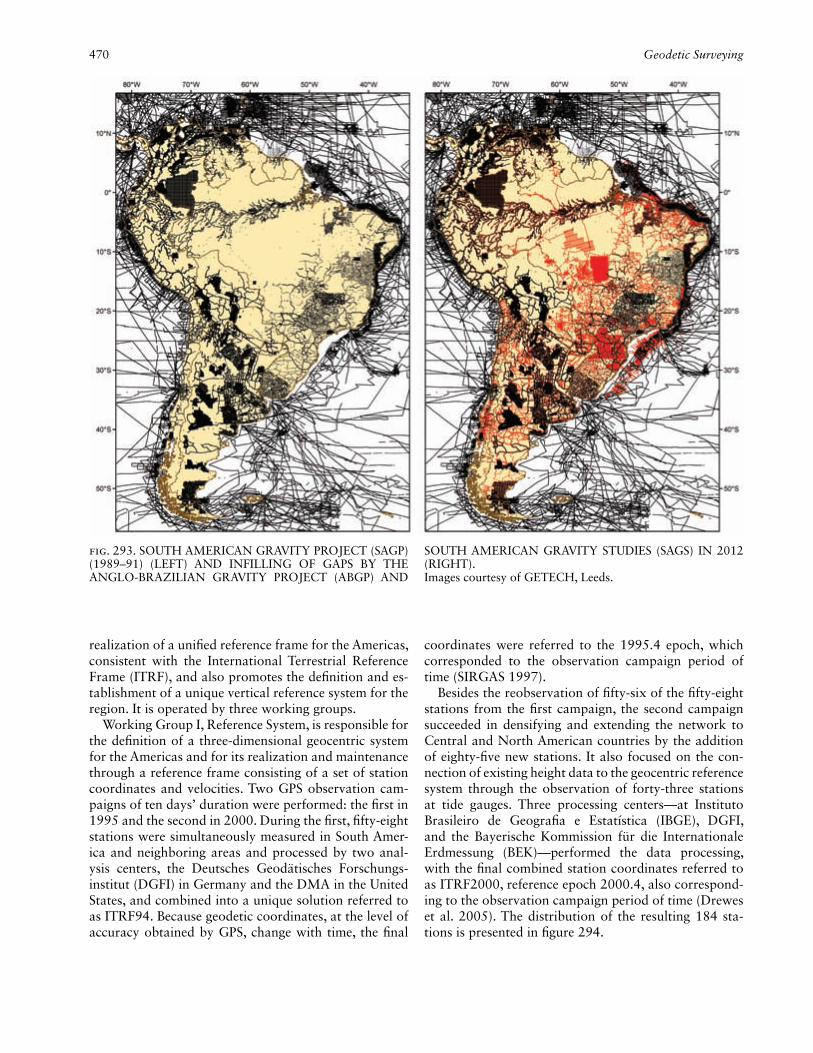
470 Geodetic Surveying

realization of a unifi ed reference frame for the Americas, consistent with the International Terrestrial Reference Frame (ITRF), and also promotes the defi nition and es-tablishment of a unique vertical reference system for the region. It is operated by three working groups.

Working Group I, Reference System, is responsible for the defi nition of a three-dimensional geocentric system for the Americas and for its realization and maintenance through a reference frame consisting of a set of station coordinates and velocities. Two GPS observation cam-paigns of ten days’ duration were performed: the fi rst in 1995 and the second in 2000. During the fi rst, fi fty-eight stations were simultaneously measured in South Amer-ica and neighboring areas and processed by two anal-ysis centers, the Deutsches Geodätisches Forschungs-institut (DGFI) in Germany and the DMA in the United States, and combined into a unique solution referred to as ITRF94. Because geodetic coordinates, at the level of accuracy obtained by GPS, change with time, the fi nal

coordinates were referred to the 1995.4 epoch, which corresponded to the observation campaign period of time (SIRGAS 1997).

Besides the reobservation of fi fty-six of the fi fty-eight stations from the fi rst campaign, the second campaign succeeded in densifying and extending the network to Central and North American countries by the addition of eighty-fi ve new stations. It also focused on the con-nection of existing height data to the geocentric reference system through the observation of forty-three stations at tide gauges. Three processing centers—at Instituto Brasileiro de Geografi a e Estatística (IBGE), DGFI, and the Bayerische Kommission für die Internationale Erdmessung (BEK)—performed the data processing, with the fi nal combined station coordinates referred to as ITRF2000, reference epoch 2000.4, also correspond-ing to the observation campaign period of time (Drewes et al. 2005). The distribution of the resulting 184 sta-tions is presented in fi gure 294.

Fig. 293. SOUTH AMERICAN GRAVITY PROJECT (SAGP) (1989–91) (LEFT) AND INFILLING OF GAPS BY THE ANGLO-BRAZILIAN GRAVITY PROJECT (ABGP) AND

SOUTH AMERICAN GRAVITY STUDIES (SAGS) IN 2012 (RIGHT).Images courtesy of GETECH, Leeds.

Fig. 294. THE GEOCENTRIC REFERENCE SYSTEM FOR THE AMERICAS, SIRGAS 2000 GPS CAMPAIGN STA-TIONS (TOTAL 184).

Image courtesy of Luiz Paulo Souto Fortes.

472 Geodetic Surveying

The maintenance of the SIRGAS reference frame is accomplished throughout the active control networks in Latin America (composed of more than eighty con-tinuously operating GPS stations in 2006), whose data are processed weekly by the IGS Regional Network As-sociate Analysis Centre for SIRGAS (IGS RNAAC-SIR) in Germany (Seemüller 2004). Working Group II, Geo-centric Datum, is in charge of the defi nition, realization, and maintenance of the geodetic datum in the member countries consistent with the SIRGAS reference frame and the promotion of the connection and transforma-tion of national geodetic networks to the geocentric datum. To date, a number of Latin American countries have offi cially adopted either SIRGAS 95 or SIRGAS 2000 as their new national reference frame. The Work-ing Group III, Vertical Datum, deals with the defi ni-tion of a modern unifi ed vertical reference system for Latin America, the establishment of the corresponding reference frame, and the transformation of the existing classical height datums to the new system (Fortes et al. 2006).

Luiz Paulo Souto Fortes and Eduardo Andrés Lauría

The authors thank Dr. Maria Cristina Barboza Lobianco for providing historical information related

to geodetic surveying in Latin America.

See also: Figure of the Earth; Geodesy; Global Positioning System (GPS); Holdich, Thomas Hungerford; Inter-American Geodetic Survey; Photogrammetric Mapping: Geodesy and Photogrammetric Mapping; Property Mapping: Property Mapping in Latin America; Tidal Measurement

Bibliography:Drewes, H., et al. 2005. “Results of the SIRGAS Campaign 2000 and

Coordinates Variations with Respect to the 1995 South American Geocentric Reference Frame.” In A Window on the Future of Ge-odesy: Proceedings of the International Association of Geodesy, ed. Fernando Sansò, 32–37. Berlin: Springer.

Fischer, Irene K. 1972. “Estructura basica del datum Sudamericano de 1969” and “The Basic Framework of the South American Datum of 1969.” Revista Cartográfi ca 21, no. 23:9–28, 29–47.

Fortes, Luiz Paulo Souto, et al. 2006. “Current Status and Future Developments of the SIRGAS Project.” In Festschift: Univ.-Prof. Dr.-Ing. Prof. h.c. Günter Seeber anlässlich seines 65. Geburtstages und der Verabschiedung in den Ruhestand, 59–70. Wissenschaft-liche Arbeiten der Fachrichtung Geodäsie und Geoinformatik der Universität Hannover 258. Hannover: Institut für Erdmessung.

Green, Christopher M., and J. Derek Fairhead. 1993. “The South American Gravity Project.” In Recent Geodetic and Gravimetric Research in Latin America, ed. Wolfgang Torge, Alvaro Gonzalez-Fletcher, and James G. Tanner, 82–95. Berlin: Springer.

Seemüller, Wolfgang. 2004. “El centro asociado de análisis del IGS para la red regional SIRGAS. IGS Regional Network Associate Analysis Centre for SIRGAS (RNAAC SIR).” Presentation at SIRGAS Tech-nical Meeting, Aguascalientes, Mexico.

Seemüller, Wolfgang, Klaus Kaniuth, and H. Drewes. 2004. Station Positions and Velocities of the IGS Regional Network for SIRGAS. Munich: Deutsches Geodätisches Forschungsinstitut.

SIRGAS. 1997. SIRGAS Final Report, Working Groups I and II. Rio de Janeiro: IBGE.

Woollard, George Prior, et al. 1967. “Catalogo de estaciones gravime-tricas en America Latina.” Geofísica Internacional 7:87–211.

Geodetic Surveying in Africa. The development of the geodetic framework of Africa, as in other parts of the world, has been closely linked to innovations in survey methods. Parts of the network based on classical survey techniques date back to the nineteenth century, and ex-tensive work was added during the 1930s and the de-cades following World War II. At the end of the twenti-eth century the quality of the network was variable, and although extended and refi ned in later years, it refl ected the initial inaccessibility of large parts of the continent as well as the varying aims and fi nancial and technical capacities of the colonial survey departments and gov-ernment agencies involved.

Broadly speaking, three types of geodetic frames can be distinguished. Of the more than fi fty African coun-tries, only a few (South Africa, some countries in East Africa situated on 30°E, Egypt, and countries in the Maghreb) boasted regular geodetic networks based on fi rst-order triangulation. By contrast, many large and arid countries situated in northwest and central Africa had networks resulting from primary traverses and iso-lated control points acquired by means of astronomical surveys alone. The third type of network was a combina-tion of the two previous survey methods and was gener-ally found in large and relatively inaccessible countries, such as the Democratic Republic of the Congo, Angola, Ethiopia, and Libya (FAO 1999). Geodetic surveying had, however, undergone a revolution since the 1970s, and by the end of the century satellite technology had begun to erase the practical problems emanating from this variable pattern.

In any discussion of the history of geodetic surveying in Africa, the Arc of the 30th Meridian takes center stage (Zakiewicz 1997). In 1879 geodesy on this continent ob-tained a champion of exceptional scientifi c vision when Sir David Gill was appointed Her Majesty’s Astronomer at the Cape of Good Hope. Realizing that no survey ex-isted in the Southern Hemisphere suffi ciently accurate to be of value for geodetic purposes, Gill immediately started negotiations with British authorities, to whom he proposed a gridiron network of trigonometric chains covering the whole of South Africa. Once this network was completed, he proposed the triangulation be ex-tended northward along the 30th degree of longitude to Cairo, from where it could be connected with F. G. W. Struve’s Russian-Scandinavian Arc. Gill kept pursuing this ideal with the utmost vigor, rendering the measure-ment of the Arc of the 30th Meridian an epic tale of almost unbelievable perseverance and dedication.

The fi rst leg of the Arc was measured from 1883 to 1892, when a team of Royal Engineers under the com-

Geodetic Surveying 473

mand of Colonel William George Morris, and with Gill’s guidance, executed the geodetic survey of Natal and the Cape Colony to a very high degree of precision. The Anglo-Boer or South African War of 1899–1902 interrupted Gill’s plans for the rest of South Africa, but in 1902 the British War Offi ce approved the geo-detic triangulation of the Transvaal and Orange River Colony, which was completed in 1906, again under the leader ship of Morris and with Gill as scientifi c adviser. As part of this survey, the Arc was carried as far north as the Limpopo River, a distance of approximately 1,600 kilometers. In the meantime, between 1897 and 1901, Alexander Simms, under Gill’s direction, extended the Arc in Southern Rhodesia (now Zimbabwe) almost to the Zambezi River. In 1906–7 Captain H. W. Gordon connected Simms’s chain to the Transvaal triangulation. The 800-kilometer section through Northern Rhodesia (now Zambia) was surveyed by the Swedish geodesist Tryggve Rubin, who in March 1906 terminated his mea-surements near the Tanganyika (now Tanzania) border for fi nancial reasons. Thus, when Gill retired from offi ce in 1907, the Arc of the 30th Meridian extended from the Cape almost to Lake Tanganyika.

From 1907 to 1909 further progress was achieved when, upon conclusion of the work of the Uganda-Congo Boundary Commission, a newly formed joint Anglo-Belgian team measured the so-called Uganda Arc from 1°N to 1°S. It was highly unfortunate that after this survey World War I and a lack of fi nances stopped work on the Arc for more than twenty years.

All along, the War Offi ce considered the completion of the Arc of primary importance. In 1931 a party of Royal Engineers, under the command of Major Mar-tin Hotine, was dispatched to carry Rubin’s chain from 10°S in Northern Rhodesia, farther north through Tan-ganyika. In 1933 Hotine took the Arc up to the border of Urundi (now Burundi) at 5°S. In 1937 the Tanganyika Survey Department completed the 400-kilometer con-nection between Urundi and Uganda, thereby extending the Arc from the Cape to the equator.

The northern segment of the Arc began in Egypt. The geodetic triangulation along the Nile commenced near Cairo in 1907, and by 1930 the Egyptian section was completed as far south as Adindan, at 22°10′N.

Due to economic problems, the measurement of the Arc across the Sudan only began in 1935, but eventually all survey work came to an end due to World War II. The work in the Sudan was resumed in 1947, and by 1952 the Abu Qarn base, at 10°N, was measured. This left a gap of approximately 1,000 kilometers in the Arc be-tween the Abu Qarn base in the Sudan and the Semliki base in Uganda of which about 500 kilometers passed through the impassable Sudd marshes. In 1952 the U.S. Army Map Service, in collaboration with the Sudan Sur-

vey Department, began this survey. In January 1954 the last gap in the Arc of the 30th Meridian was closed—Sir David Gill’s dream of a continuous Arc from the Cape to Cairo had at last become a reality (fi g. 295). Unfor-tunately, the seventy-fi ve years that had elapsed since its initiation had by then impaired the usefulness of the Arc insofar as new electronic distance-measuring instru-ments had come into use and satellite technology was making the measurement of arcs for geodetic purposes obsolete. The U.S. Army Map Service did, however, use the results of the Arc for the computation of a new fi g-ure of the earth, and even before the fi nal closure, ad-justments were carried out for various sections of the Arc. The adjustment for the section between Southern Rhodesia and Uganda was conducted by the British Di-rectorate of Overseas Surveys, the results of which were termed the New 1950 Arc Datum (McGrath 1983). Referenced to the Clarke 1880 ellipsoid, this datum, together with its slightly different successor, the 1960 Arc Datum, became the foundation of all surveying and mapping work in East and Central African countries. Likewise, the Geodetic Survey of South Africa was based on the Cape Datum, which was referenced to the Modi-fi ed Clarke 1880 ellipsoid—a situation that lasted until January 1999, when the new South African Hartebeest-hoek 94 Datum (referenced to the WGS 84 ellipsoid) came into use.

South African portionorganized by Sir David Gill

completed in 1907

Major Martin Hotine1931 to March 1933

Tanganyika Survey Department, 1938

Uganda Arc, Anglo-Belgian Commission, 1908–9

U.S. Army Map ServiceDecember 1952 to January 1954

Sudan Survey Department, 1930–51

Egyptian triangulation, 1907–30

Fig. 295. THE MEASUREMENT OF THE ARC OF THE 30TH MERIDIAN, 1883 TO 1954.

474 Geodetic Surveying

Meanwhile geodetic work in the rest of Africa was conducted in a piecemeal fashion. From 1924 to 1936 Egypt ran a geodetic chain from Cairo westward along the coast as far as Tripoli and eastward up to the bor-der with Palestine. During the 1880s and 1890s France, which had a strong presence in northwest Africa since the middle of the nineteenth century, commissioned its Service géographique de l’armée to undertake a geodetic triangulation in Tunisia and Algeria. Connecting chains covering the coastal area of Morocco were added dur-ing the 1920s. Until 1940, when it was superseded by the Institut géographique national (IGN), the Service géographique de l’armée was also responsible for the geodetic infrastructure (mainly primary traverses and astronomical observations) of francophone West and Equatorial Africa (Finsterwalder and Hueber 1943).

Before World War II the most notable geodetic work in the Belgian Congo (now Democratic Republic of the Congo) was undertaken by the Comité spécial du Ka-tanga (CSK), a privately managed state agency founded in 1919. The mining activities in the Katanga (now Shaba province) necessitated geodetic control, and by 1942 southern and eastern Katanga had been triangulated and the network linked to the Arc of the 30th Meridian in Tanganyika and Northern Rhodesia (Finsterwalder and Hueber 1943). After the establishment of the Institut géographique du Congo Belge (IGCB) in 1949 the geo-detic network was extended westward to link Katanga to the Angolan coast. From 1960 until 1972 extensive ad-justments along this link resulted in the establishment of the so-called Arc of the 6th Parallel (south) (Meex 1997).

Between 1885 and 1915 Germany undertook geo-detic surveying in German South-West Africa (Namibia) and German East Africa (Tanzania). The German agen-cies concerned were the Königliche Preußische Landes-aufnahme and its civilian successor, the Reichsamt für Landesaufnahme. In German South-West Africa an east-west geodetic chain, initially measured between Swakop-mund and Gobabis, was extended to the Okavango River in the north and the Orange River in the south (Finsterwalder and Hueber 1943). This framework was in use until the 1980s, when the South African Chief Directorate of Surveys and Mapping undertook a sat-ellite resurvey of the geodetic network of Namibia. In German East Africa, an Anglo-German Boundary Com-mission (1902–6) observed a primary chain along the border with Kenya, and in 1912–14 a network of pri-mary triangles was established in the east of the colony (Rowe 1933, 173).

From 1883 until 1911 surveying in Angola and Mo-çambique (Mozambique) was organized by the Portu-guese Ministério da Marinha e Ultramar, which assigned this responsibility to the Comissão de Cartographia. In 1911 this ministry was divided into the Ministério da Marinha and the Ministério das Colónias. From 1951

to 1974 the latter ministry was known as the Ministé-rio do Ultramar. Until 1951 the Ministério das Colónias coordinated the work of the Comissão de Cartographia, which often collaborated with the Portuguese army for the surveying of terrestrial areas. One such survey was a geodetic triangulation that was performed in Moçam-bique from 1932 to 1936 (Finsterwalder and Hueber 1943). Geodetic measurements were also made in An-gola, but the particulars are unknown. After 1936 until independence geodetic work was regulated by the Junta das Missões Geográfi cas e de Investigações Coloniais (JMGIC), a department of the Ministério do Ultramar.

Apart from the work done by boundary commis-sions and the work on the Arc of the 30th Meridian, little geodetic work was undertaken in British Africa in the interwar years (Winterbotham and McCaw 1928; McGrath 1976). The necessity of survey frameworks for development was, however, realized (Worthington 1938, 36), and during the 1930s the Colonial Survey Com-mittee commissioned the measuring of various geodetic chains in Uganda, Tanganyika, the Gold Coast (Ghana), and Nigeria (McGrath 1976; Rowe 1933; Calder Wood 1936). In 1946 effective central control over the survey-ing and mapping of British dependencies was at long last reached with the establishment of the Directorate of Colonial (later Overseas) Surveys. During the 1950s and early 1960s primary chains were measured in Uganda, Kenya, Nyassaland (Malawi), Northern Rhodesia, and Basutoland (Lesotho) as well as in Nigeria, Sierra Le-one, and Gambia in West Africa (McGrath 1983). In Tan ganyika the original German observations executed before World War I were recomputed and embodied in a new triangulation scheme, and in Bechuanaland (Botswana) a primary framework was observed using Tellurometer traverses. Until 1984, when it was incor-porated into the Overseas Surveys Directorate of the British Ordnance Survey, the Directorate of Overseas Surveys undertook valuable work in maintaining and extending geodetic networks on the continent.

Since the 1970s the use of satellite systems such as the U.S. Navy Navigation Satellite System (NNSS), the Navstar Global Positioning System (GPS), and the Rus-sian GLONASS (Global’naya Navigatsionnaya Sput-nikovaya Sistema) for position fi xing radically altered the nature of geodetic surveying. Worldwide, this new technology led to increased international cooperation in geodesy and the development of unifi ed geodetic frameworks. The latter became especially necessary in Africa, where the continent’s colonial heritage accounts for survey systems of different countries based on dif-ferent datums referenced to different spheroids. Early in the twenty-fi rst century an African initiative called the African Geodetic Reference Frame (AFREF) sought to alter this situation by creating a network of continu-ous, permanent GPS stations throughout the continent

Geodetic Surveying 475

(Wonnacott 2005). In 2001, the project gained the for-mal support of the International Association of Geodesy (IAG) and the United Nations Economic Commission for Africa (UNECA), which saw AFREF as a key step toward a precise geoid for Africa and a uniform and consistent coordinate system for the entire continent.

Elri Liebenberg

See also: Figure of the Earth; Geodesy; Global Positioning System (GPS); Holdich, Thomas Hungerford; Photogrammetric Mapping: Geodesy and Photogrammetric Mapping; Property Mapping: Af-rica; Tidal Measurement

Bibliography:Calder Wood, J. 1936. “The Survey Framework of Nigeria.” Empire

Survey Review 3:386–95, 450–59, and 4:65–82.Finsterwalder, Richard, and Ernst Hueber. 1943. Vermessungswesen

und Kartographie in Afrika. Berlin: Walter de Gruyter.Food and Agricultural Organization of the United Nations (FAO).

1999. AFRICOVER: Specifi cations for Geometry and Cartography. Environment and Natural Resource Series, no. 1. Rome: Food and Agricultural Organization. Online publication.

McGrath, Gerald. 1976. The Surveying and Mapping of British East Africa, 1890 to 1946: Origins, Development and Coordination. Monograph 18, Cartographica. Toronto: B. V. Gutsell.

———. 1983. Mapping for Development: The Contributions of the Directorate of Overseas Surveys. Monograph 29–30, Cartographica 20, nos. 1–2.

Meex, Pierre. 1997. “Historique du réseau triangulé au Congo belge/Zaïre.” Bulletin des Séances/Bulletin de l’Académie Royale des Scien ces d’Outre-Mer 43:193–215.

Rowe, H. P. 1933. “Triangulation in Tanganyika Territory.” Empire Survey Review 2:171–77.

Winterbotham, H. S. L., and G. T. McCaw. 1928. “The Triangulations of Africa.” Geographical Journal 71:16–36.

Wonnacott, Richard. 2005. “AFREF: Background and Progress to-wards a Unifi ed Reference System for Africa.” Proceedings of the International Federation of Surveyors (FIG) Working Week and GSDI-8 Conference, Cairo, Egypt, 16–21 April 2005. Online publication.

Worthington, E. Barton. 1938. Science in Africa: A Review of Scien-tifi c Research Relating to Tropical and Southern Africa. London: Oxford University Press.

Zakiewicz, Tomasz. 1997. “The African Arc of the 30th Meridian.” South African Journal of Surveying and Mapping 24:65–82.

Geodetic Surveying in Europe. The geodetic activi-ties in Europe at the beginning of the twentieth century were guided by the International Association of Geod-esy (IAG) constitution of 1886. National institutions responsible for geodetic surveying followed the IAG rec-ommendations related to the establishment of geodetic networks, whose main purpose was to support carto-graphic coverage of the countries. The IAG was a succes-sor of the Europäische Gradmessung, subsequently the Internationale Erdmessung, a group of twenty nations. During World War I the Internationale Erdmessung was dissolved, and in 1919 the International Union of Geod-esy and Geophysics was founded (Levallois 1988; Torge 1993).

Until the introduction of space geodetic techniques the prescribed methodology consisted of establishing

triangulation networks. The layout was either a con-tinuous net or a system of chains. The latter was ini-tially adopted by the majority of the countries, given its lower costs and implementation time. The geometry of triangulation networks was defi ned by angles or direc-tion measurements using highly accurate theodolites. The orientation was controlled by the establishment of Laplace stations at selected sites where astronomical ob-servations for azimuth and longitude were performed. The scale of the triangulation networks was given by the length measurement of selected sides.

An important development that improved distance measurement was the discovery of invar, an iron-nickel alloy, near the end of the nineteenth century. Its low co-effi cient of thermal expansion made it desirable for the measurement of baselines, replacing wooden and other metal rulers and tapes. The invar wires were used un-til the introduction of the electronic distance meters or electromagnetic distance measurement (EDM) in the middle of the twentieth century. EDM instruments were used to measure the sides of the geodetic networks. In countries where the network was sparse, traverses were used to replace triangulations or to control the scale of the network as, for example, in Finland (Parm 1976). To maintain the scale consistency of the instruments Väisälä baselines were established in almost all coun-tries of Europe and in many other areas of the world for instrument calibration. The lengths of these baselines were determined very accurately by the multiplication of a very precise optical length reference.

Until World War II the different European nations each developed their own geodetic reference systems or geodetic datums. They were based on the choice of a ref-erence ellipsoid, a point of origin, and associated param-eters: astronomical latitude and longitude, north-south (ξ) and east-west (η) components of the defl ection of the vertical, astronomical azimuth of one direction, and the geoid undulation (N).

The reconstruction of Europe after the war moti-vated the integration of these datums into a common one. Primary triangulation chains were selected by the Western European countries to form a continuous net-work, the Réseau Européen 1950 (fi g. 296). The U.S. Coast and Geodetic Survey computed the network, and the resulting coordinates were referred to as ED50 (Eu-ropean Datum 1950), which had its origin point at the Helmertturm in Potsdam, Germany. At this point were assigned the values of the vertical defl ection components (ξ = 3.36 arc seconds, η = 1.78 arc seconds) and the geoid undulation (N = 0 m). The associated reference spheroid was the International ellipsoid, determined by John Fillmore Hayford and adopted by the International Union of Geodesy and Geophysics in 1924; its param-eters are the semimajor axis a = 6,378,388 meters and the fl attening f = 1/297. Many countries adopted ED50

476 Geodetic Surveying

as the offi cial geodetic datum, serving as a basis for their cartographic and surveying activities.

In 1954 the IAG created the subcommission RETrig (Réseau Européen Trigonométrique). Its main purpose was to continue the computation of the European geo-detic network and to increase its quality, including new

and more accurate measurements. A new version of the European Datum was adopted in 1979 (ED79) based on dense triangulation networks (Kobold 1980). The im-portance of including Doppler observations in the next phase of the computations was recognized at that time, and they were fi nished in 1987 when a new solution,

Fig. 296. RÉSEAU EUROPÉEN, 1:6,000,000, 1949. There are several versions of the network and map.

Size of the original: 72.8 × 67.7 cm. Image courtesy of the Cartothèque, Institut géographique national.

Geodetic Surveying 477

ED87, was adopted. The work of RETrig was very fruit-ful and contributed to the development of computation techniques.

Many Eastern European countries, integrated with the former Soviet Union, adopted the Pulkovo Datum of 1942, with its origin at the Pulkovo Observatory. The 1942 Krasovskiy ellipsoid, defi ned by the semima-jor axis a = 6,378,245 meters and the fl attening f = 1/298.3, was adopted as the reference surface.

The development of the vertical datums in Europe followed the approaches of the geodetic networks very closely. At the beginning of the twentieth century several tide gauges had already been installed to pro-vide a reference for heights (vertical datums) in each country or group of countries. Leveling lines were es-tablished in order to fulfi ll particular needs, and grav-ity measurements were also performed to reduce spirit leveling observations. The countries adopted different height systems. For instance, normal heights are used in France and Sweden, orthometric heights in Finland and Spain, and normal-orthometric heights in Austria and Norway.

In 1955 the REUN (Réseau Européen Unifi é de Ni-vellement) commission of the IAG initiated its work aimed at the unifi cation of Western European leveling networks. The computations were performed in geopo-tential heights and the origin was the Normaal Amster-dams Peil in Amsterdam. Each country selected the most appropriate leveling lines to fulfi ll the accuracy require-ments and the need for continuous loops across the re-gion. The fi rst solution, REUN 1957, was computed and followed by several others until the late 1980s, when REUN was discontinued. The work was continued later by the EUREF (European Reference Frame) subcommis-sion. G. Bomford (1980) provided details concerning the instrumentation and techniques used in the establish-ment of classical horizontal and vertical datums.

Artifi cial satellites were used for geodetic purposes in Europe very early. In the 1960s a set of observation projects were performed using satellites Echo 1, Echo 2, and PAGEOS (Passive Geodetic Earth Orbiting Satellite) launched by the U.S. National Aeronautics and Space Administration. In 1963 the French and Algerian net-works were connected. This test campaign was extended in 1965 by the connection of the Portuguese mainland and the Azores archipelago networks (fi g. 297). In 1967 a new connection was established between Europe (France) and Africa (Senegal and Chad). Spatial trian-gulation was used allowing for the fi rst time the con-nection of networks at long distances (Levallois 1988, 247–65).

At the end of the 1960s the fi rst measurements were made of distances to artifi cial satellites and to the moon using laser beams and telescopes. This technique is known as satellite laser ranging (SLR) or lunar laser

ranging (LLR), and its applications in the fi elds of earth dynamics, gravity fi eld, and rotation are all crucial for establishing accurate global geocentric reference frames. Another space technique contributing to the reference frame maintenance is the VLBI (very long baseline inter-ferometry), developed in the 1970s. This technique uses the determination of the distance between two radio telescopes that receive radio signals from a quasar. By the end of the twentieth century about twelve SLR sites and ten VLBI sites operated in Europe. Some observa-tories integrated several space geodetic techniques (e.g., Matera in Italy and Wettzell in Germany).

The fi rst Doppler observation, EDOC-1 (European Doppler Observation Campaign), took place in 1975 and used the satellites of the Transit constellation. In 1977 EDOC-2 was organized, consisting of thirty-nine stations in fi fteen countries, and resulted in a set of homogeneous coordinates in Europe close to a quasi- geocentric global geodetic system.

The Navstar GPS (Global Positioning System) suc-ceeded the Transit system as a geodetic tool in the mid-dle of the 1980s. The high accuracy and reliability of the GPS made it suitable for establishing a new refer-ence frame covering the whole European continent, re-placing the ED solutions. Recognizing the potential of space-based geodetic techniques for the establishment and maintenance of global and continental geodetic ref-erence frames and the need for a modern and precise continental reference frame in Europe, the IAG consti-

Fig. 297. CONNECTION EUROPE–AZORES USING THE SATELLITE ECHO 1. Image shows the locations of photo-graphic observations in 1965.Size of the original : 8.1 × 8 cm. From Levallois 1988, 257 (fi g. 108).

478 Geodetic Surveying

tuted the EUREF subcommission in 1987 to continue the work of RETrig under this new perspective.

In 1990, EUREF defi ned the ETRS89 (European Ter-restrial Reference System 1989) as a system with the origin at the earth’s center of mass and tied to the sta-ble part of the Eurasian plate (EUREF 1990). The cor-responding reference frame was conceived as the geo-detic infrastructure for multinational projects requiring precise georeferencing. The ETRS89 is tied to the ITRS (International Terrestrial Reference System), maintained and made available by the IERS (International Earth Ro-tation Service), which also produces the corresponding ITRF (International Terrestrial Reference Frame) and the relationships among the different frames. The IERS was established in 1987 by the International Astronomi-cal Union and the International Union of Geodesy and Geophysics, replacing the International Polar Motion Service and the earth-rotation section of the Bureau In-ternational de l’Heure.

A set of markers homogeneously covering the Eu-ropean continent was established by EUREF to make the ETRS89 available to the users. The EUREF89 GPS campaign, the fi rst one at the continental level, was or-ganized in 1989, allowing the determination of ETRS89 coordinates of ninety-two stations across Western Eu-rope. After the end of the Cold War the Eastern Euro-pean countries joined EUREF efforts, resulting in cover-age of all but three European countries.

In 1996 the EPN (EUREF Permanent Network) was created. By the end of the twentieth century about 120 stations were integrated into the EPN. This covered the European continent homogeneously and made continuous observations with high accuracy GPS receiv-ers (fi g. 298). The EPN is a densifi cation of the Interna-tional GPS Service and contributes to the ITRS and the monitoring of tectonic deformations in Europe.

At about the same time, EUREF was charged to con-tinue the work of REUN and produce the UELN95/98 (Unifi ed European Levelling Network) solution. This was extended to the majority of the Eastern European countries and defi ned as the EVRS (European Vertical Reference System) to express the height information.

A link between the vertical and geospatial compo-nents was established in 1997 through the EUVN97 (European Vertical GPS Reference Network), a Europe-wide GPS campaign consisting of 196 sites collocated at nodal points of the UELN and near tide gauges. As a result, the parameters were obtained to transform the national height systems into a common European height reference system (Ádám et al. 2002).

Geodetic surveying in Europe was carried out by the national mapping agencies of each country. These insti-tutes were generally civilian. In the 1980s the European national mapping agencies formed CERCO (Comité Eu-

ropéen des Responsables de la Cartographie Offi cielle), later transformed into the EuroGeographics consortium including the cadastral agencies as well. The research activities in geodesy were carried out by geodetic insti-tutes and laboratories at university and governmental research sites.

During the twentieth century European geodesists and institutions published a considerable number of textbooks (e.g., Bomford 1980; Levallois 1969–71; Jor-dan, Kneissl, and Eggert 1956–72). They also contrib-uted to technical journals and reports. Notable technical journals included Allgemeine Vermessungs-Nachrichten (Germany), Bollettino di Geodesia e Scienze Affi ni (It-aly), Geodeziya i Aerofotos”yëmka (Russia), and Survey Review (United Kingdom). Important report series were Suomen geodeettisen laitoksen julkaisuja (Finland), Publications on Geodesy (Netherlands), and the publica-tions of the Deutsche Geodätische Kommission bei der Bayerischen Akademie der Wissenschaften (Germany).

João Agria Torres

See also: Figure of the Earth; Geodesy; Global Positioning System (GPS); Photogrammetric Mapping: Geodesy and Photogrammetric Mapping; Property Mapping: Europe; Tidal Measurement

Bibliography:Ádám, József, et al. 2002. “Status of the European Reference Frame—

EUREF.” In Vistas for Geodesy in the New Millennium: IAG 2001

Fig. 298. GPS TRACKING STATIONS OF THE EUREF PER-MANENT NETWORK IN JUNE 2000.From Carine Bruyninx, “Overview of the EUREF Permanent Network and the Network Coordination Activities,” presented at EUREF Symposium, June 22–24, 2000, Tromsø, Norway, fi g. 1 (online publication). Permission courtesy of Dr. Carine Bruyninx, Royal Observatory of Belgium, Brussels.

Geodetic Surveying 479

Scientifi c Assembly, Budapest, Hungary, September 2–7, 2001, ed. József Ádám and Klaus-Peter Schwarz, 42–46. Berlin: Springer.

Bomford, G. 1980. Geodesy. 4th ed. Oxford: Clarendon Press.EUREF. 1990. “Report on the Symposium of the IAG Subcommission

European Reference Frame (EUREF) in Florence from May 28 to 31, 1990.” Veröffentlichungen der Bayerischen Kommission für die Internationale Erdmessung der Bayerischen Akademie der Wissen-schaften: Astronomisch-geodätische Arbeiten 52:15–95.

Jordan, Wilhelm, Max Kneissl, and Otto Eggert. 1956–72. Hand-buch der Vermessungskunde. 10th ed. 6 vols. in 16. Stuttgart: J. B. Metzler.

Kobold, Fritz, ed. 1980. The European Datum 1979 (ED79): Report on the Symposium of the IAG Subcommission for the New Adjust-ment of the European Triangulation (RETrig), held in Madrid from 7 to 12 May 1979. Munich: Deutsches Geodätisches Forschungsin-stitut.

Levallois, Jean-Jacques. 1969–71. Géodésie générale. 4 vols. Paris: Eyrolles.

———. 1988. Mesurer la Terre: 300 ans de géodésie française, de la toise du Châtelet au satellite. Paris: Presses de l’Ecole Nationale des Ponts et Chaussées.

Parm, Teuvo. 1976. High Precision Traverse of Finland. Helsinki: n.p.Torge, Wolfgang. 1993. “Von der mitteleuropäischen Gradmessung

zur Internationalen Assoziation für Geodäsie.” Zeitschrift für Ver-messungswesen 118:595–605.

Geodetic Surveying in Russia and the Soviet Union. During the twentieth century, the Russian geodetic sur-vey service operated throughout the vast area of the country, covering more than 22,000,000 square kilome-ters. Most of its territory consisted of sparsely populated or virgin mountain terrain, taiga, tundra, wetlands with many rivers and lakes, and a broad area of permafrost.

In 1897 Korpus voyennykh topografov (KVT), the corps of military topographers—the service that carried out the majority of topographic and geodetic surveys in the Russian Empire—completed the adjustment of the fi rst-order triangulation series, which was estab-lished in the country in the nineteenth century. Apart from the KVT, geodetic surveying was also conducted by Mezhevoye vedomstvo (the estate surveying depart-ment); Gornoye vedomstvo (the mining department); Pereselencheskoye upravleniye (administration for the development of Eastern Russian agricultural lands and resettlement of European Russians to them); Gidrogra-fi cheskoye upravleniye (the hydrographic administration of the admiralty); Ministerstvo putey sobshcheniya (the ministry of transportation); Imperatorskoye Russkoye geografi cheskoye obshchestvo (IRGO, the imperial Rus-sian geographical society); and a number of other agen-cies. However, their activities had little impact on the mapping of the country’s territory because they were not coordinated. Triangulation was carried out indepen-dently in every province, with different control points used in each project, resulting in substantial coordinate discrepancies at the junctions of triangulation networks. The adjustment of the fi rst-order triangulation failed to eliminate the discrepancies, making apparent the

inadequate state of triangulation in Russia. Therefore, in 1910, the KVT conducted a new fi rst-order geodetic survey, which put an end to the chaotic development of fi rst-order triangulation in Russia. Despite its limited personnel (in 1906 the corps consisted of 513 topog-raphers and geodetic surveyors), the KVT produced a substantial body of work. However, given the vastness of the country, it was not enough (see fi g. 1017). More-over, by the end of World War I, a substantial number of the geodetic networks established by the KVT came to be located outside Russian borders (Sudakov 1975).

On many occasions a number of prominent Russian scholars and public fi gures argued for the establishment of a national geodetic service. Their proposals were dis-cussed at the meetings of the Akademiya nauk and the RGO; however the idea was successfully implemented only after the Bolshevik Revolution of 1917.

In March 1919, despite the raging civil war and col-lapsing economy, a governmental decree established the Vyssheye geodezicheskoye upravleniye (VGU) for the topographic exploration of the country’s territory (see table 18 for the name changes of this organization during the twentieth century). During the twentieth century, the VGU closely collaborated with Voyenno- topografi cheskaya sluzhba (the military topographic service), and all geodetic projects had to meet technical requirements jointly approved by the two institutions.

By 1923 the Soviet geodetic survey service had begun to carry out systematic triangulation and topographic surveys at 1:50,000 scale, primarily in central parts of Russia, Ukraine, the Volga region, and the Ural Moun-tains. As the state could not provide suffi cient funding and the geodetic survey service lacked both qualifi ed personnel and high-precision instruments, the projects were of limited scope. For that reason, in the 1920s the geodetic survey service concentrated more on analyzing the results of earlier works and on establishing basic principles for future projects. After careful consideration some very important decisions were made: the fi rst-order triangulation networks were transformed into an astronomical-geodetic network; the Bessel spheroid was adopted for geodetic network calculations; the zero mark of the Kronstadt tide gauge (on the Baltic Sea) was adopted as the vertical datum; the Gauss-Krüger orthog-onal coordinate system was adopted as standard; and a new system of dividing topographic maps into sheets was introduced. In order to facilitate and speed up sur-veying, 1:50,000 and 1:100,000 scales were adopted as standard for national surveys, rather than the 1:25,000 scale that was preferred by some governmental agencies. Feodosiy Nikolayevich Krasovskiy, a leading geodesist, estimated that it would take between 100 and 150 years to map central Russia if the scale of 1:25,000 had been adopted.

480 Geodetic Surveying

Extremely important events for the Soviet geodetic survey service included: the establishment of Tsentral’nyy nauchno-issledovatel’skiy institut geodezii, aeros”yëmki i kartografi i (TsNIIGAiK, the scientifi c research institute of geodesy and cartography), Moskovskiy geodeziches-kiy institut (MGI), which was later named Moskov-skiy institut inzhenerov geodezii, aerofotos”yëmki i kartografi i (MIIGAiK, the Moscow institute of geodetic engineering, aerial photography, and cartography), and several technical schools for geodesy; the adoption of air photography for topographic surveys; and the onset of geodetic instrument production in the country. The fi rst-order national triangulation scheme and program was developed by Krasovskiy and ensured the necessary precision of the traverse networks (Sudakov 1967).

In the 1930s, the country went through rapid indus-trialization and the collectivization of agriculture. The demand for geodetic networks was so high that the geodetic survey service lacked the resources to meet it. Many institutions carrying out geodetic surveys and projects emerged following their own guidelines. The general condition of geodetic networks was considered unsatisfactory due to these numerous digressions from adopted schemes and schedules. Typical surveys con-ducted between 1929 and 1935 show that guidelines were poorly coordinated and projects overlapped. The adjustment of leveling and triangulation networks, car-ried out between 1932 and 1935, revealed a 1.875-meter divergence between European and Siberian leveling. The disparity in a point’s position between the Pulkovo coor-dinate system adopted in the western part of the country and the Svobodnyy coordinate system in its eastern part was up to 270 meters in latitude and up to 790 meters in longitude (Kashin 1999). There was little alternative, for a period at least, to retaining the Pacifi c system of altitudes in Siberia, as well as the Svobodnyy, Magadan, Tashkent, and other coordinate systems, along with the Pulkovo one.

From 1926 to 1935, while undergoing numerous re-organizations and losing its independence, the geodetic survey service failed to reach its main goal, which was to reconcile the competing interests of various agencies (which instead prevailed over the general interests of the Soviet states) and to coordinate their topographic and geodetic projects. In 1935 and 1938 the Soviet government reorganized the geodetic survey service. It established Glavnoye upravleniye geodezii i kartografi i (GUGK), subordinate to the Soviet security police and responsible for the mapping of the country’s territory. The geodetic survey service considerably improved its material resources and organized the manufacturing of high-precision surveying instruments. The size of its per-sonnel also steadily increased. It would not be an ex-aggeration to suggest this was the period when Soviet

geodesy and cartography entered its golden age, which lasted until the late 1980s (see fi gs. 1018–20). Between 1931 and 1944, 180 engineers and technicians entered the ranks of the geodetic survey service every year, while more than 1,000 specialists in this fi eld had graduated from secondary schools and higher institutions by 1975. By 1985 the total number of engineering and technical personnel in the geodetic survey service had reached 25,000.

In this period, which lasted more than fi fty years, the Soviet geodetic survey service developed a mod-ern astronomic-geodetic network (AGN) covering the whole territory of the Soviet Union and characterized by its high density and uniformity. Its creation enabled the geodetic survey service to achieve its two main ob-jectives within a relatively short period: to complete in less than twenty years the mapping of the country at 1:100,000 scale and to produce in less than thirty years topographic maps for the whole country at 1:25,000 scale. It was possible because of considerable advance-ments in science, the development of a modern surveying instrument manufacturing industry, photogrammetry, computing technology, a widespread implementation of aerospace methods, improved organization of topo-graphic and geodetic projects, and the dedication of the geodetic survey service personnel.

From 1938 to 1940 the major guidelines for topo-graphic and geodetic projects were standardized (ta-ble 17). The Osnovnyye polozheniya o postroyenii gosudarstvennoy opornoy geodezicheskoy seti SSSR, indispensable regulations for establishing the state geo-detic control network, were implemented (fi g. 299). These could be used for geodetic control of surveying at 1:10,000 scale. The construction of geodetic networks and topographic surveying was concentrated in the Eu-ropean part of the country and Western Siberia. First-order triangulation was also carried out in the Far East, in Kazakhstan, and in Central Asia.

From June 1941, when Nazi Germany attacked the Soviet Union, the major aim of the Soviet geodetic survey service was to provide the army with maps and catalogs of coordinates and to carry out surveys in strategically important areas (Baranov and Kudryavtsev 1967). Even before victory over Nazi Germany, the geodetic survey service began to restore damaged geodetic networks, to update maps, and to develop networks for surveys of industrial areas of the country at 1:10,000 scale, and at 1:100,000 scale for other areas.

In 1946, after a scheduled adjustment of the fi rst-order triangulation and the leveling control network, a governmental decree introduced uniform systems of geodetic coordinates and heights—the 1942-System with the Pulkovo datum point and the Baltic Height Sys-tem with the Kronstadt tide gauge as the datum point.

Geodetic Surveying 481

The Krasovskiy reference ellipsoid (semimajor axis = 6,378,245 meters; fl attening ratio = 1/298.3) was ad-opted for calculating geodetic points.

The AGN point coordinates, which had been earlier established within regional systems, were recalculated for the 1942-System. This encompassed the entire Euro-pean part of the Soviet Union, Kazakhstan, Central Asia, and Western Siberia, while stretching further eastward as a narrow belt to the Far East. From the mid-1950s to the late 1960s major projects were carried out in the northern and eastern regions of the country, where inten-sive exploitation of natural resources was taking place. It was essential to construct the AGN for the whole ter-ritory of the Soviet Union and to develop second- and third-order geodetic networks for surveys at 1:25,000 and 1:10,000 scales and extensive networks for surveys at 1:5,000 scale and larger (Sudakov 1967). In the early 1970s the geodetic survey service completed the adjust-ment of the AGN on a block-by-block basis; a single coordinate system was adopted for the whole country.

The application of visible and radio wavelength elec-tromagnetic distance measurement equipment enabled the transition to the construction of second- and third-order polygon networks to replace existing triangula-tion networks. The geodetic survey service expanded its surveys considerably at scales between 1:10,000 and 1:2,000 for land reclamation purposes. Fourth-order short-sided polygons formed the main geodetic basis for topographic surveying at the scales of 1:5,000 and larger. In the late 1960s the application of optic and ra-dio technology in surveying enabled the development of the space geodetic network (SGN). All SGN points were integrated with the AGN points and were used for subsequent network adjustment. The global navigation system, GLONASS (Global’naya Navigatsionnaya Sput-

Table 17. Topographic surveys in the Soviet Union completed by the outbreak of the Great Patriotic War, 1941–45

ScaleArea surveyed to 1918 (km2)

Area surveyed 1918–32 (km2)

Area surveyed 1933–37 (km2)

Area surveyed 1938–40 (km2) Total

1:10,000 or larger 1,800 139,500 179,700 8,100 329,100

1:21,000 13,100 7,400 1,200 1,200 22,900

1:25,000 - 259,300 273,200 65,700 598,200

1:42,000 98,600 49,400 - - 148,000

1:50,000 - 644,300 189,700 400,000 1,234,000

1:84,000 541,600 139,500 - - 681,100

1:100,000 - 550,500 408,200 370,700 1,329,400

1:200,000 - 30,300 344,300 160,600 535,200

Total 655,100 1,820,200 1,396,300 1,006,300 4,877,900

Fig. 299. DIAGRAM FROM OSNOVNYYE POLOZHE-NIYA O POSTROYENII GOSUDARSTVENNOY OPOR-NOY GEODEZICHESKOY SETI SSSR, 1939, SHOWING THE GEODETIC NETWORK OF THE SOVIET UNION. The key at the bottom identifi es fi rst-, second-, and third-order triangulation sides (left) and fi rst-order points, baselines, and Laplace stations (right).From Sudakov 1967, 70.

482 Geodetic Surveying

nikovaya Sistema), was also created. At the same time much work was done in high-risk seismic areas of the country, where the geodetic survey service carried out repeated leveling and established geodynamic test areas for periodic high-precision geodetic surveys in order to trace pre-earthquake warning signs.

In the 1950s and 1960s the Soviet geodetic survey service carried out substantial topographic and geo-detic surveys in the western parts of China and in Syria, Afghanistan, Iraq, and Indonesia. Since the 1970s the GUGK actively collaborated with geodetic survey ser-vices of developing nations by training their personnel, supplying equipment, and carrying out aerial surveys, and topographic, geodetic, and cartographic projects. The most important projects, such as developing geodetic networks and making and updating topographic maps, were conducted in Cuba, Nicaragua, Mongolia, Afghan-istan, Laos, Yemen, Somalia, Angola, Mozambique, and Ethiopia. Collaboration with other countries was partic-ularly strong in using data produced by remote sensing. The Soviet geodetic survey service took part in mapping the moon and other planets of the solar system. In 1970 the GUGK began its work in the Antarctic, where Soviet research stations carried out observations of the space-based geodetic complex, established control gravimetric points, and conducted large-scale topographic surveys (Natsional’nyy otchet geodezicheskoy sluzhby SSSR za ’89, 1990).

In the mid-1970s the observation of the fi rst-order state gravimetric network began. Moscow, Lyodovo, St. Petersburg (Leningrad), and Irkutsk were included as fundamental points in the World Gravimetric System. Gravimetric surveying was also carried out on the con-tinental shelf. The adjustment of the state gravimetric network was completed in 1986.

The AGN was completed in the 1980s and consisted of 164,360 fi rst- and second-order triangulation points. The network was supplemented with 170,000 third- and fourth-order extension geodetic network points, which served as the major geodetic basis for the whole range of topographic surveys, beginning with a scale of 1:500 (Kashin 1999). From 1983 to 1993, in order to increase the precision of the AGN, the Doppler Geodetic Net-work (DGN) was created in its weakest points by apply-ing the Transit navigation system; its 134 points were evenly distributed across the country’s territory, being combined with the AGN points.

In 1992 a unifi ed Soviet geodetic survey service ceased to exist. Due to reduced funding allocated to the Rus-sian geodetic survey service, the scope of its projects was reduced considerably, and high-precision gravimetric surveying, shelf topographic surveying, and other proj-ects in the Antarctic were virtually abandoned.

During the last decade of the twentieth century, the AGN was adjusted. Autonomous methods for coordinat-ing satellites involving the widely used global navigation systems GLONASS and GPS (Global Positioning Sys-tem) were introduced into topographic and geodetic sur-veying. Also introduced were digital technologies for the production and revision of topographic maps and plans at scales ranging from 1:500 to 1:1,000,000. By the mid-1990s the total coverage of leveling networks exceeded 600,000 kilometers, of which more than 160,000 kilo-meters were fi rst-order leveling networks. The sched-uled general adjustment of the fi rst- and second-order state leveling networks was also carried out. From 1995 to 1996, as a result of a joint adjustment of the AGN, SGN, and DGN, a new high-precision reference system of geodetic coordinates, SK-95, was established aimed at covering the whole territory of Russia with equal pre-cision. The SGN is an implementation of a geocentric coordinate system, which is part of the global system of the earth’s geodetic parameters (PZ-90). Thus, high-pre-cision geodetic coordinate systems were created, the ref-erential system SK-95 and the geocentric system PZ-90, with securely established parameters of mutual position-ing. Adjusted values of AGN point coordinates allow suffi cient precision in establishing uniform parameters of transition to the geodetic coordinate systems PZ-90 and WGS84, within which the satellite systems GLONASS and GPS operate (Brovar et al. 1999).

Alexsandr Sudakov

See also: Figure of the Earth; Geodesy; Global Positioning System (GPS); Moskovskiy institut inzhenerov geodezii, aerofotos”yëmki i kartografi i (Moscow Institute of Geodetic Engineering, Aerial Photo graphy, and Cartography; Russia); Photogrammetric Map-ping: Geodesy and Photogrammetric Mapping; Property Mapping: Russia and the Soviet Union; Tidal Measurement; Tsentral’nyy nauchno-issledovatel’skiy institut geodezii, aeros”yëmki i karto-grafi i (Central Research Institute of Geodesy, Air Survey, and Car-tography; Russia)

Bibliography:Baranov, A. N., and M. K. Kudryavtsev. 1967. “Geodeziya i karto-

grafi ya na sluzhbe sotsialisticheskogo stroitel’stva i oborony strany.” In 50 let sovetskoy geodezii i kartografi i, ed. A. N. Baranov and M. K. Kudryavtsev, 7–20. Moscow: Nedra.

Brovar, B. V., et al. 1999. “Sostoyaniye i perspektivy razvitiya sistemy geodezicheskogo obespecheniya strany v usloviyakh perekhoda na sputnikovyye metody.” Geodeziya i kartografi ya, no. 1:29–33.

Kashin, L. A. 1999. Postroyeniye klassicheskoy astronomo-geode-zicheskoy seti Rossii i SSSR (1816–1991 gg.). Moscow: Kartgeo-tsentr-Geodezizdat.

Kudryavtsev, M. K., Yu V. Sergovskiy, and S. A. Salyayev. 1967. “Geo-deziya i kartografi ya v gody grazhdanskoy i Velikoy Otechestven-noy voyn.” In 50 let sovetskoy geodezii i kartografi i, ed. A. N. Bara-nov and M. K. Kudryavtsev, 141–63. Moscow: Nedra.

Leninskiy dekret v deystvii: 60 let sovetskoy geodezii i kartografi i. 1979. Moscow: GUGK.

Natsional’nyy otchet geodezicheskoy sluzhby SSSR za ’89. 1990. Mos-cow: GUGK.

Geodetic Surveying 483

Natsional’nyy otchet kartografo-geodezicheskoy sluzhby Rossii za 1992 god. 1993. Moscow: TsNIIGAiK.

Sudakov, S. G. 1967. “Osnovnyye topografo-geodezicheskiye raboty za 50 let sovetskoy vlasti.” In 50 let sovetskoy geodezii i kar-tografi i, ed. A. N. Baranov and M. K. Kudryavtsev, 21–90. Moscow: Nedra.

———. 1975. Osnovnyye geodezicheskiye seti. Moscow: Nedra.

Geodetic Surveying in Australia. Geodetic survey made little progress in Australia in the fi rst half of the twentieth century because of the country’s vast size and fragmented approach to land survey. Local trigonomet-ric surveys initiated in the individual colonies in the 1830s had stalled by the time of Federation in 1901 be-cause of a shortage of surveyors, who also had to meet the needs of land grants, roads, civil projects, town sites, ports, and coastal surveys. Cadastral surveys were not linked to a national framework, and geodetic survey re-mained a low national priority, leaving Australia with a number of different geodetic origins and datums, such as the Everest spheroid and several Clarke spheroids.

The fi rst meeting of state surveyors general, held in 1912, identifi ed an integrated geodetic survey as its top priority. However, little was achieved until 1932, when the Royal Australian Survey Corps became operational and commenced a fi rst-order triangulation chain from South Australia across Victoria and through eastern New South Wales (fi g. 300). This endeavor tied together individual state networks and led to the adoption of

Sydney Observatory as the origin for all mapping in eastern Australia (FitzGerald 1934).

In 1945 state and federal bodies established the Na-tional Mapping Council. A resolution passed at the council’s fi rst meeting recognized the variable quality of state networks, which were largely unrecoverable, and identifi ed completion of the geodetic triangulation as a top national priority. Although a small National Mapping offi ce was established within the federal gov-ernment in 1947 and trigonometric observations com-menced in 1951, progress was hampered by limited vis-ibility in fl at, featureless terrain. Because ground control was urgently needed, military and civilian fi eld parties used astronomical observations to fi x positions in re-mote areas of the continent so that topographic map-ping could proceed in parallel with the geodetic survey (Hocking 1985).

In the second half of the twentieth century geodesy advanced markedly beyond the triangulation techniques perfected by the Survey of India. The introduction of elec-tronic distance measuring (EDM) equipment in the 1950s, electronic computers in the 1960s, and satellite position-ing in the 1970s heralded a transition from datums based on regional best-fi t ellipsoids to global datums and com-plex approximations of the geoid. By the end of the cen-tury, geodesy in Australia was using permanent Global Positioning System (GPS) installations to monitor move-ment of the Australian tectonic plate (approximately 6 cm per year) and offering rapid online computation of GPS observations on a geocentric datum.

The reliance on triangulation techniques to establish the Australian geodetic framework was overcome when Bruce Philip Lambert, director of National Mapping, in-troduced EDM equipment, fi rst the Geodimeter in 1954 and then the Tellurometer in 1957. New techniques for distance measurements and loop traverses, controlled by reciprocal azimuth observations, were quickly devel-oped, and a geodetic framework was established across the continent by the end of 1965 (Ford 1979).

Field data from 2,506 stations, including 533 Laplace astronomical stations, established along 53,000 kilome-ters of Tellurometer traversing posed a massive mathe-matical challenge, which was undertaken in 1966 using mainframe computers. Positions were computed accord-ing to a best-fi t local spheroid, the Australian National Spheroid, which was assumed to coincide with the geoid at its origin point, the Johnston Geodetic Station (Bom-ford 1967; Lambert 1968). The newly computed posi-tions were accepted by the National Mapping Coun-cil as the Australian Geodetic Datum 1966 (AGD66), which provided the fi rst homogeneous positional data set across the country, a remarkable achievement in just ten years (fi g. 301).

Fig. 300. STATUS OF FIRST- AND SECOND-ORDER TRI-ANGULATIONS IN 1945.Size of the original: 7.3 × 7.7 cm. From Lambert 1968, 127 (fi g. II). © 1968 United Nations.

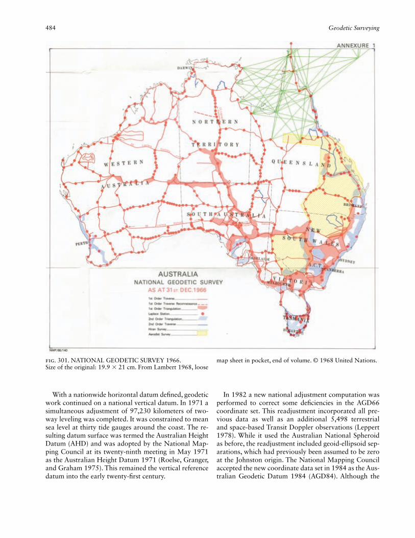
484 Geodetic Surveying

With a nationwide horizontal datum defi ned, geodetic work continued on a national vertical datum. In 1971 a simultaneous adjustment of 97,230 kilometers of two-way leveling was completed. It was constrained to mean sea level at thirty tide gauges around the coast. The re-sulting datum surface was termed the Australian Height Datum (AHD) and was adopted by the National Map-ping Council at its twenty-ninth meeting in May 1971 as the Australian Height Datum 1971 (Roelse, Granger, and Graham 1975). This remained the vertical reference datum into the early twenty-fi rst century.

In 1982 a new national adjustment computation was performed to correct some defi ciencies in the AGD66 coordinate set. This readjustment incorporated all pre-vious data as well as an additional 5,498 terrestrial and space-based Transit Doppler observations (Leppert 1978). While it used the Australian National Spheroid as before, the readjustment included geoid-ellipsoid sep-arations, which had previously been assumed to be zero at the Johnston origin. The National Mapping Council accepted the new coordinate data set in 1984 as the Aus-tralian Geodetic Datum 1984 (AGD84). Although the

Fig. 301. NATIONAL GEODETIC SURVEY 1966.Size of the original: 19.9 × 21 cm. From Lambert 1968, loose

map sheet in pocket, end of volume. © 1968 United Nations.

Geodetic Surveying 485

council recognized the need for Australia to eventually adopt a geocentric datum, it was not clear at that time which reference ellipsoid to use.

With the introduction of GPS in the late 1980s the need arose for improved accuracy in the geodetic frame-work and a transition to an earth-centered datum, in which the spheroid is aligned with the earth’s center of mass rather than with a point of origin on the earth’s surface. This strategy, which permits a more even dis-tribution of separations between the spheroid and the geoid, required the development and application of new techniques to ensure direct compatibility with coordi-nates based on satellite positioning. A new framework with a geocentric origin was based on eight continuous GPS stations whose positions were established using the International Terrestrial Reference Frame (as calculated for the 1 January 1994 epoch). The adjustment was also based on systematic GPS observations at additional sta-tions used for the 1984 datum and all former terrestrial observations (Steed 1995). Calculations were carried out using least-squares adjustment software developed by Australia’s Department of Resources and Energy.

For a large country like Australia, the shift to an earth-centered datum can make sheet boundaries quaintly (if not radically) obsolete for existing quadrangle maps, to-gether with the parallels and meridians shown thereon. Because previous positions had been calculated on a local (rather than earth-centered) fi gure of the earth, the Geocentric Datum of Australia 1994 (GDA94) and its coordinate sets required a variable shift of roughly 200 meters for coordinates across Australia (fi g. 302).

Relating new and old coordinate systems required the computation of spatial-transformation grids for each state (Collier, Argeseanu, and Leahy 1998). With this massive task complete, GDA94 was introduced across the country in 2000 as a joint project of the state and federal governments (Manning 2006).

John Manning

See also: Figure of the Earth; Geodesy; Global Positioning System (GPS); Photogrammetric Mapping: Geodesy and Photogrammetric Mapping; Property Mapping: Australia and New Zealand; Tidal Measurement

Bibliography:Bomford, A. G. 1967. “The Geodetic Adjustment of Australia, 1963–

1966.” Survey Review 19:52–71.Collier, P.A., V. S. Argeseanu, and F. J. Leahy. 1998. “Distortion Model-

ling and the Transition to GDA94.” Australian Surveyor 43:29–40.FitzGerald, Lawrence. 1934. “The Co-ordination of the Trigonometri-

cal Surveys of Queensland, New South Wales, Victoria and South Australia.” Australian Surveyor 5:22–31.

Ford, R. A. 1979. “The Division of National Mapping’s Part in the Geodetic Survey of Australia.” Australian Surveyor 29:375–427, 465–536, and 581–638.

Hocking, David R. 1985. “Star Tracking for Mapping—An Account of Astrofi x Surveys by the Division of National Mapping during 1948–1952.” In Technical Papers: 27th Australian Survey Congress, Alice Springs, 1985, 13–27. N.p.: Institution of Surveyors, Australia.

Lambert, Bruce Philip. 1968. “The Geodetic Survey of Australia.” In Fifth United Nations Regional Cartographic Conference for Asia and the Far East, 8–22 March 1967, Canberra, Australia, 2 vols., 2:126–31. New York: United Nations.

Leppert, K. 1978. The Australian Doppler Satellite Survey, 1975–1977. Canberra: Department of National Development, Division of Na-tional Mapping.

Lines, John D. 1992. Australia on Paper: The Story of Australian Map-ping. Box Hill, Victoria: Fortune Publications.

Manning, John. 2006. “The Geodetic Survey of Australia.” In 400 Years of Mapping Australia: Darwin Conference, 23 to 25 August 2006: Author Papers & Biographies. CD-ROM, paper 8. [Darwin, N.T.]: MSIA.

Roelse, A., H. W. Granger, and J. W. Graham. 1975. The Adjustment of the Australian Levelling Survey, 1970–1971. 2d ed. Canberra: De-partment of Minerals and Energy, Division of National Mapping.

Steed, Jim. 1995. “The Geocentric Datum of Australia.” Surveying World 4, no. 1:14–17.

Geodetic Surveying for the Planets. The advent of plan-etary exploration in the twentieth century encouraged car-tographers to map extraterrestrial bodies, which led to a host of conceptual and technological challenges. The mak-ing of the earliest planetary maps required the processing of digital images transmitted from spacecraft or collected from telescopic observations, assembling those images into a photomosaic, and then, in the earliest maps, manu-ally painting a picture of the planetary surface on a map projection. Even this inexact process of mapmaking, made easier with better spacecraft and computers, required the solution of several geodetic problems that were less than trivial, and much different from those encountered by ter-restrial cartographers (Greeley and Batson 1990).

207

205

201

194206

204

204

204

207

207

Fig. 302. COORDINATE SHIFTS IN METERS FROM AGD84 TO GEOCENTRIC DATUM 1994.After Manning 2006.

486 Geodetic Surveying

The fi rst challenge was that of geodetic control. On the surface of the earth, geodetic control points, used as refer-ence locations, are typically established by land survey or satellite photography. This process was more troublesome in planetary mapping because it was diffi cult to establish the precise locations of landmarks either using satellite or telescopic imagery. In early extraterrestrial cartography most of the control points used for planets and smaller bodies like the moon were the centers of impact craters defi ned by centroid calculations based on their rims (Da-vies 1990, 141). These networks were diffi cult to establish with any degree of accuracy and were computed using an-alytical photogrammetry. In 1958 the Austrian astronomer G. Schrutka-Rechtenstamm used telescopic observations to calculate the fi rst modern geodetic control network for the moon. The base of this network was the crater Möst-ing A, a location suggested by the astronomer F. W. Bessel as early as 1839. During the 1970s satellites like Mariner, Viking, and Voyager provided data that allowed reference networks to be established on Mars, Jupiter, and Saturn.

The second problem encountered in early planetary mapping concerned topography, the calculation of which presented a series of interrelated problems. In earth mapping, elevations are referenced to sea level, which does not exist elsewhere and therefore had to be artifi cially defi ned. Also, the control networks that were established on extraterrestrial surfaces were not as ac-curate as those devised for the earth, which made it dif-fi cult not only to fi x locations precisely and reference photographic images but also to calculate the planet’s shape. Both of these problems were central to the es-tablishment of a topographic datum or geoid to which topographic features could be referenced.

Establishing a reference geoid for the planets was a highly mathematical endeavor requiring careful mea-surement and the use of spherical harmonics. The geoid used for earth is the equipotential surface on which gravity is constant and corresponds to mean sea level. To establish an equipotential surface for a planet like Mars, which has no readily available physical analog like the sea, required gravity measurements. Because no gravity measurements existed for solar system bod-ies in the 1970s, the defl ection of the orbiting satellite’s path as it passed over various topographic features like mountains, craters, and canyons was carefully tracked and used to calculate the equipotential surface.

The accurate determination of the shape of the plan-ets was also important. According to the laws of physics, any elastic body that rotates around a fi xed axis will as-

sume the shape of what is known as an ellipsoid of equi-librium. Depending on the size of the planet, the ma-terial properties of its mass, and its rotational velocity, various forms of the ellipsoid are possible. The composi-tion and rotational velocities of the planets vary greatly, from the giant gaseous Jupiter, which rotates quickly, to rocky worlds like Venus, which rotates much more slowly. In order to map these shapes, more fl exible map projections were developed so that the planets could be mapped conformally and their cartographic features then transferred easily to other map projections. One ap-proach allowed the shape of the ellipsoid to vary along its three axes, thus providing a general projection useful for a wide variety of planetary shapes (Snyder 1985).

As the investigations of the planets expanded during the 1970s, the mapping of smaller bodies like asteroids, comets, and satellites required unprecedented map pro-jections (fi g. 303). Because of their low mass and typi-cally slow rotational velocities, these bodies lack the gravitational force needed to form fi gures of equilib-rium and thus have extremely irregular shapes. The fi rst projections for irregular bodies developed in the early 1970s utilized cylindrical projections and were limited to a narrow range of applications; they gave good repre-sentations of the circumequatorial regions of the body if it was moderately ellipsoidal but contained massive dis-tortions if the shape was more complex, as it is for many asteroids and small moons. Sculptor Ralph J. Turner (1978) developed the fi rst truly useful model for Mars’s closest moon Phobos, based on an azimuthal projection. Geographers Philip J. Stooke and C. Peter Keller (1987) mathematically modifi ed Turner’s projection to form a conformal projection useful for nonspherical worlds.

John W. Hessler

See also: Astrophysics and Cartography; Figure of the Earth; Geod-esy; Lunar and Planetary Mapping; Mathematics and Cartography; Tidal Measurement

Bibliography:Chandrasekhar, S. 1969. Ellipsoidal Figures of Equilibrium. New Ha-

ven: Yale University Press.Davies, Merton E. 1978. “The Control Net of Mars: May 1977.” Jour-

nal of Geophysical Research 83, no. B5:2311–12.———. 1990. “Geodetic Control.” In Planetary Mapping, ed. Ronald

Greeley and Raymond M. Batson, 141–68. Cambridge: Cambridge University Press.

Greeley, Ronald, and Raymond M. Batson, eds. 1990. Planetary Map-ping. Cambridge: Cambridge University Press.

Schrutka-Rechtenstamm, G. 1958. “Neureduktion der 150 Mond-punkte der Breslauer Messungen von J. Franz.” Sitzungsberichte, Österreichische Akademie der Wissenschaften, Mathematisch-naturwissenschaftliche Klasse, Abt. II, 167:71–123.

(Facing page)Fig. 303. NONSPHERICAL PROJECTION FOR PHOBOS. Mars’s moons were the fi rst small and irregularly shaped ob-jects to be photographed in detail and at high resolution. Con-

sequently they have often been the test cases for new mapping methods.Image courtesy of Philip J. Stooke, University of Western Ontario.

488 Geographic Information System

Snyder, John Parr. 1985. “Conformal Mapping of the Triaxial Ellip-soid.” Survey Review 28:130–48.

Stooke, Philip J., and C. Peter Keller. 1987. “Morphographic Projec-tions for Maps of Non-spherical Worlds.” Lunar and Planetary Sci-ence 18:956–57.

Turner, Ralph J. 1978. “Modeling and Mapping Phobos.” Sky and Telescope 56:299–303.

Geografi cheskoye obshchestvo SSSR (Geographical Society of the USSR). See Russkoye geografi cheskoye obshchestvo (Russian Geographical Society)

Geographic Information System (GIS).Computational Geography as a New

ModalityGIS as an Institutional RevolutionGIS as a Tool for Map Analysis and Spatial

ModelingGIS as a Tool for Map ProductionMetadata

Computational Geography as a New Modality. By the end of the twentieth century, computer-based appli-cations of geographic information science and technol-ogy were widespread in many areas of human endeavor. Spatial, and increasingly spatial-temporal, factors were recognized as decisive in many phases of personal and societal planning and decision making. This stands in sharp contrast to the situation prevailing earlier in the century, when the role of spatial factors was poorly un-derstood, and the limited availability of spatial data and tools for spatial analysis and visualization severely re-stricted the ability to deal with spatial problems on an effective operational level. To understand and appreciate the revolutionary change during the last four decades of the twentieth century requires an awareness of the very different circumstances that prevailed prior to the ad-vent of geographic information system (GIS) technology.

Geographic space, as well as the heterogeneous distri-bution of resources within that space, exerts a signifi cant and complex infl uence on human behavior and the spa-tial structure of society. Attempts to identify and under-stand the content of the geographic space that encom-passes us, as well as the way that geographic space, as abstracted from the things contained within it, impacts human behavior have engaged humans on an informal level for most of our existence. The development of more formal views of these concerns forms the basis for the modern science of geography. The great extent and high complexity of the space that humans occupy pre-sents substantial barriers to its understanding. The early, ultimately successful effort to create a conceptually for-mal and operationally viable method of recording and reproducing representations of distant, out-of-sight por-tions of earth-space in the form of maps introduced a

new, highly signifi cant modality into geography through the introduction of cartography. The impact of this new modality was characterized by Arthur H. Robinson as something “as profound as the invention of a number system” (1982, 1). The complex concepts underlying the creation and use of maps, such as scale, projection, and symbology, have challenged cartographers and the us-ers of maps ever since, as have the substantial problems involved in the acquisition of the very large volumes of spatial data needed to characterize and understand the world.

Analog maps proved to be highly useful, both con-ceptually and in practice, but they possess inherent limi-tations with respect to the amount of spatial data that can be accommodated. The basic workfl ow of spatial data acquisition, analog map creation, map storage, and extraction and ultimate use of the stored spatial data is highly labor and resource intensive. The traditional map restricts the level of analysis of its stored spatial data that can be supported when only the human eye-brain system serves as the primary extraction and analysis tool. A few aids (e.g., for measuring distance and direc-tion) were developed to assist visual analysis, but any signifi cant ability to deal with diffi cult spatial questions was lacking given the extraordinary amount of time and resources required to generate the desired answers.

When responses to diffi cult spatial questions are not easily obtained, these questions often end up not being posed. The resulting myopic views became widespread within the intellectual community and within the realm of practical geographic applications. Consequently, po-tentially important concepts relating to the role of spa-tial factors in shaping individual and societal behavior were implicitly relegated to the category “out of sight, out of mind.” The subsequent failure to pose diffi cult questions created a profound, and mostly unrecognized, constraint upon our conceptual views of space and hu-man behavior. The role of distance in human interaction was a subject for limited discourse, but usually within the context of a simplifi ed two-dimensional isotropic space; a space that was often further simplifi ed by an implicit reduction to a single dimension (i.e., dealing with distance but not direction). Also falling below the intellectual horizon in geography and cartography were even more complex questions that required explicit con-sideration of time as well as space (Peuquet 2002). The interaction between these limited conceptual views and the minimal tools available for acquisition and analysis of spatial data is reminiscent of Ouroboros and obvi-ously, in retrospect, awaited a revolutionary new modal-ity to break the vicious circle of concepts limiting tools and tools limiting concepts.

In the early 1960s developing computer technology began to be applied to store and manipulate digital rep-resentations of spatial data (Hershey 1963; Horwood

Geographic Information System 489

et al. 1963). Development of specialized graphic output capabilities revealed the potential for fl exible creation and display of many different forms of maps. The early computer-generated maps were simple ones, and their creation required, at the time, very substantial resources (e.g., Tobler 1959). The potential for fl exibility in scale, map projection, symbology, etc., became evident as, somewhat later, did the ability to create previously underutilized cartographic representations (e.g., carto-grams), the manual creation of which involved inordi-nate levels of effort (Harness 1838; Wright 1936; Skoda and Robertson 1972; Tobler 2004).

The potential for enhancing spatial analysis within a computational environment was also emerging, and early efforts by Edgar M. Horwood (Horwood et al. 1963) and others (e.g., Hägerstrand 1967; Marble and Anderson 1972; Baxter 1976) demonstrated that com-putational approaches to spatial analysis were not only viable but were capable of illuminating new conceptual horizons (fi g. 304). Initial attempts at computation-based spatial analysis encountered major diffi culties due to the lack of knowledge of how to represent spatial data within the computer and the lack of useful spatial analysis algorithms. Much of the early conceptual work undertaken involved the challenging formalization of existing cartographic notions and the equally diffi cult adaptation of simplistic spatial analysis approaches to the far more challenging problems posed by a highly heterogeneous space. Early computational efforts often relied upon local “hand crafted” software solutions that were laborious to utilize and diffi cult to transfer else-where. Attempts to create interoperable computer-based solutions (e.g., Marble 1967) were inhibited by the ma-

jor differences existing in computer hardware and oper-ating systems.

The initially limited supply of digital spatial data also proved to be a major impediment in the conceptual and operational adoption of computer-based spatial analy-sis and mapping approaches. There appeared to be no viable way to convert even a portion of the existing analog spatial data into useable digital form (e.g., the generation of structured topological databases instead of what A. Raymond Boyle so neatly labeled a “bowl of spaghetti”). Major problems were also encountered with attribute categorizations used in existing maps that had only minimal utility when viewed within a broader operational context. During the late 1970s and early 1980s the data conversion bottleneck slowly dimin-ished, fi rst through Boyle’s invention of the free-cursor digitizer and by the subsequent development of reliable high-speed scanners.

The conversion of analog maps posed two major prob-lems: development of the electromechanical hardware for “reading” analog maps and creation of the software needed to translate the captured analog data into reus-able digital form. In retrospect, conceptual issues un-derlying creation of the software proved to be a greater intellectual challenge than development of the hardware (Peuquet and Boyle 1984). Efforts toward direct digital data acquisition by remote sensing, and the later intro-duction of Global Positioning Systems (GPS), induced major changes, and by the early 1990s the spatial data supply situation had begun moving from a severe drought to a fl ood that would challenge existing capabilities.

The early development of integrated software systems designed to store, manipulate, analyze, and display spa-

BBBBBBBBBBBBBBBBBBBBBBBBBBBBBBBBBBBBBBBBBBBBBBBBBBBBBBBBBBBBBBBBBBBBBBBBBBBBBBBBBBBBBBBBBBBBBBBBBBBBBBBBBBBBBBBBBBBBBBBBBBBBBBBBBBBBBBBBBBBBBBBBBBBBBBBBBBBBBBBBBBBBBBBBBBBBBBBBBBBBBBBBBBBBBBBBBBBBBBBBBBBBBBBBBBBBBBBBBBBBBBBBBBBBBBBBBBBBBBBBBBBBBBBBBBBBBBBBBBBBBBBBBBBBBBBBBBBBBBBBBBBBBBBBBBBBBBBBBBBBBBBBBBBBBBBBBBBBBBBBBBBBBBBBBBBBBBBBBBBBBBBBBBBBBBBBBBBBBBBBBBBBBBBBBBBBBBBBBBBBBBBBBBBBBBBBBBBBBBBBBBBBBBBBBBBBBBBBBBBBBBBBBBBBBBBBBBBBBBBBBBBBBBBBBBBBBBBBBBBBBBBBBBBBBBBBBBBBBBBBBBBBBBBBBBBBBBBBBBBBBBBBBBBBBBBBBBBBBBBBBBBBBBBBBBBBBBBBBBBBBBBBBBBBBBBBBBBBBBBBBBBBBBBBBBBBBBBBBBBBBBBBBBBBBBBBBBBBBBBBBBBBBBBBBBBBBBBBBBBBBBBBBBBBBBBBBBBBBBBBBBBBBBBBBBBBBBBBBBBBBBBBBBBBBBBBBBBBBBBBBBBBBBBBBBBBBBBBBBBBBBBBBBBBBBBBBBBBBBBBBBBBBBBBBBBBBBBBBBBBBBBBBBBBBBBBBBBBBBBBBBBBBBBBBBBBBBBBBBBBBBBBBBBBBBBBBBBBBBBBBBBBBBBBBBBBBBBBBBBBBBBBBBBBBBBBBBBBBBBBBBBBBBBBBBBBBBBBBBBBBBBBBBBBBBBBBBBBBBBBBBBBBBBBBBBBBBBBBBBBBBBBBBBBBBBBBBBBBBBBBBBBBBBBBBBBBBBBBBBBBBBBBBBBBBBBBBBBBBBBBBBBBBBBBBBBBBBBBBBBBBBBBBBBBBBBBBBBBBBBBBBBBBBBBBBBBBBBBBBBBBBBBBBBBBBBBBBBBBBBBBBBBBBBBBBBBBBBBBBBBBBBBBBBBBBBBBBBBBBBBBBBBBBBBBBBBBBBBBBBBBBBBBBBBBBBBBBBBBBBBBBBBBBBBBBBBBBBBBBBBBBBBBBBBBBBBBBBBBBBBBBBBBBBBBBBBBBBBBBBBBBBBBBBBBBBBBBBBBBBBBBBBBBBBBBBBBBBBBBBBBBBBBBBBBBBBBBBBBBBBBBBBBBBBBBBBBBBBBBBBBBBBBBBBBBBBBBBBBBBBBBBBBBBBBBBBBBBBBBBBBBBBBBBBBBBBBBBBBBBBBBBBBBBBBBBBBBBBBBBBBBBBBBBBBBBBBBBBBBBBBBBBBBBBBBBBBBBBBBBBBBBBBBBBBBBBBBBBBBBBBBBBBBBBBBBBBBBBBBBBBBBBBBBBBBBBBBBBBBBBBBBBBBBBBBBBBBBBBBBBBBBBBBBBBBBBBBBBBBBBBBBBBBBBBBBBBBBBBBBBBBBBBBBBBBBBBBBBBBBBBBBBBBBBBBBBBBBBBBBBBBBBBBBBBBBBBBBBBBBBBBBBBBBBBBBBBBBBBBBBBBBBBBBBBBBBBBBBBBBBBBBBBBBBBBBBBBBBBBBBBBBBBBBBBBBBBBBBBBBBBBBBBBBBBBBBBBBBBBBBBBBBBBBBBBBBBBBBBBBBBBBBBBBBBBBBBBBBBBBBBBBBBBBBBBBBBBBBBBBBBBBBBBBBBBBBBBBBBBBBBBBBBBBBBBBBBBBBBBBBBBBBBBBBBBBBBBBBBBBBBBBBBBBBBBBBBBBBBBBBBBBBBBBBBBBBBBBBBBBBBBBBBBBBBBBBBBBBBBBBBBBBBBBBBBBBBBBBBBBBBBBBBBBBBBBBBBBBBBBBBBBBBBBBBBBBBBBBBBBBBBBBBBBBBBBBBBBBBBBBBBBBBBBBBBBBBBBBBBBBBBBBBBBBBBBBBBBBBBBBBBBBBBBBBBBBBBBBBBBBBBBBBBBBBBBBBBBBBBBBBBBBBBBBBBBBBBBBBBBBBBBBBBBBBBBBBBBBBBBBBBBBBBBBBBBBBBBBBBBBBBBBBBBBBBBBBBBBBBBBBBBBBBBBBBBBBBBBBBBBBBBBBBBBBBBBBBBBBBBBBBBBBBBBBBBBBBBBBBBBBBBBBBBBBBBBBBBBBBBBBBBBBBBBBBBBBBBBBBBBBBBBBBBBBBBBBBBBBBBBBBBBBBBBBBBBBBBBBBBBBBBBBBBBBBBBBBBBBBBBBBBBBBBBBBBBBBBBBBBBBBBBBBBBBBBBBBBBBBBBBBBBBBBBBBBBBBBBBBBBBBBBBBBBBBBBBBBBBBBBBBBBBBBBBBBBBBBBBBBBBBBBBBBBBBBBBBBBBBBBBBBBBBBBBBBBBBBBBBBBBBBBBBBBBBBBBBBBBBBBBBBBBBBBBBBBBBBBBBBBBBBBBBBBBBBBBBBBBBBBBBBBBBBBBBBBBBBBBBBBBBBBBBBBBBBBBBBBBBBBBBBBBBBBBBBBBBBBBBBBBBBBBBBBBBBBBBBBBBBBBBBBBBBBBBBBBBBBBBBBBBBBBBBBBBBBBBBBBBBBBBBBBBBBBBBBBBBBBBBBBBBBBBBBBBBBBBBBBBBBBBBBBBBBBBBBBBBBBBBBBBBBBBBBBBBBBBBBBBBBBBBBBBBBBBBBBBBBBBBBBBBBBBBBBBBBBBBBBBBBBBBBBBBBBBBBBBBBBBBBBBBBBBBBBBBBBBBBBBBBBBBBBBBBBBBBBBBBBBBBBBBBBBBBBBBBBBBBBBBBBBBBBBBBBBBBBBBBBBBBBBBBBBBBBBBBBBBBBBBBBBBBBBBBBBBBBBBBBBBBBBBBBBBBBBBBBBBBBBBBBBBBBBBBBBBBBBBBBBBBBBBBBBBBBBBBBBBBBBBBBBBBBBBBBBBBBBBBBBBBBBBBBBBBBBBBBBBBBBBBBBBBBBBBBBBBBBBBBBBBBBBBBBBBBBBBBBBBBBBBBBBBBBBBBBBBBBBBBBBBBBBBBBBBBBBBBBBBBBBBBBBBBBBBBBBBBBBBBBBBBBBBBBBBBBBBBBBBBBBBBBBBBBBBBBBBBBBBBBBBBBBBBBBBBBBBBBBBBBBBBBBBBBBBBBBBBBBBBBBBBBBBBBBBBBBBBBBBBBBBBBBBBBBBBBBBBBBBBBBBBBBBBBBBBBBBBBBBBBBBBBBBBBBBBBBBBBBBBBBBBBBBBBBBBBBBBBBBBBBBBBBBBBBBBBBBBBBBBBBBBBBBBBBBBBBBBBBBBBBBBBBBBBBBBBBBBBBBBBBBBBBBBBBBBBBBBBBBBBBBBBBBBBBBBBBBBBBBBBBBBBBBBBBBBBBBBBBBBBBBBBBBBBBBBBBBBBBBBBBBBBBBBBBBBBBBBBBBBBBBBBBBBBBBBBBBBBBBBBBBBBBBBBBBBBBBBBBBBBBBBBBBBBBBBBBBBBBBBBBBBBBBBBBBBBBBBBBBBBBBBBBBBBBBBBBBBBBBBBBBBBBBBBBBBBBBBBBBBBBBBBBBBBBBBBBBBBBBBBBBBBBBBBBBBBBBBBBBBBBBBBBBBBBBBBBBBBBBBBBBBBBBBBBBBBBBBBBBBBBBBBBBBBBBBBBBBBBBBBBBBBBBBBBBBBBBBBBBBBBBBBBBBBBBBBBBBBBBBBBBBBBBBBBBBBBBBBBBBBBBBBBBBBBBBBBBBBBBBBBBBBBBBBBBBBBBBBBBBBBBBBBBBBBBBBBBBBBBBBBBBBBBBBBBBBBBBBBBBBBBBBBBBBBBBBBBBBBBBBBBBBBBBBBBBBBBBBBBBBBBBBBBBBBBBBBBBBBBBBBBBBBBBBBBBBBBBBBBBBBBBBBBBBBBBBBBBBBBBBBBBBBBBBBBBBBBBBBBBBBBBBBBBBBBBBBBBBBBBBBBBBBBBBBBBBBBBBBBBBBBBBBBBBBBBBBBBBBBBBBBBBBBBBBBBBBBBBBBBBBBBBBBBBBBBBBBBBBBBBBBBBBBBBBBBBBBBBBBBBBBBBBBBBBBBBBBBBBBBBBBBBBBBBBBBBBBBBBBBBBBBBBBBBBBBBBBBBBBBBBBBBBBBBBBBBBBBBBBBBBBBBBBBBBBBBBBBBBBBBBBBBBBBBBBBBBBBBBBBBBBBBBBBBBBBBBBBBBBBBBBBBBBBBBBBBBBBBBBBBBBBBBBBBBBBBBBBBBBBBBBBBBBBBBBBBBBBBBBBBBBBBBBBBBBBBBBBBBBBBBBBBBBBBBBBBBBBBBBBBBBBBBBBBBBBBBBBBBBBBBBBBBBBBBBBBBBBBBBBBBBBBBBBBBBBBBBBBBBBBBBBBBBBBBBBBBBBBBBBBBBBBBBBBBBBBBBBBBBBBBBBBBBBBBBBBBBBBBBBBBBBBBBBBBBBBBBBBBBBBBBBBBBBBBBBBBBBBBBBBBBBBBBBBBBBBBBBBBBBBBBBBBBBBBBBBBBBBBBBBBBBBBBBBBBBBBBBBBBBBBBBBBBBBBBBBBBBBBBBBBBBBBBBBBBBBBBBBBBBBBBBBBBBBBBBBBBBBBBBBBBBBBBBBBBBBBBBBBBBBBBBBBBBBBBBBBBBBBBBBBBBBBBBBBBBBBBBBBBBBBBBBBBBBBBBBBBBBBBBBBBBBBBBBBBBBBBBBBBBBBBBBBBBBBBBBBBBBBBBBBBBBBBBBBBBBBBBBBBBBBBBBBBBBBBBBBBBBBBBBBBBBBBBBBBBBBBBBBBBBBBBBBBBBBBBBBBBBBBBBBBBBBBBBBBBBBBBBBBBBBBBBBBBBBBBBBBBBBBBBBBBBBBBBBBBBBBBBBBBBBBBBBBBBBBBBBBBBBBBBBBBBBBBBBBBBBBBBBBBBBBBBBBBBBBBBBBBBBBBBBBBBBBBBBBBBBBBBBBBBBBBBBBBBBBBBBBBBBBBBBBBBBBBBBBBBBBBBBBBBBBBBBBBBBBBBBBBBBBBBBBBBBBBBBBBBBBBBBBBBBBBBBBBBBBBBBBBBBBBBBBBBBBBBBBBBBBBBBBBBBBBBBBBBBBBBBBBBBBBBBBBBBBBBBBBBBBBBBBBBBBBBBBBBBBBBBBBBBBBBBBBBBBBBBBBBBBBBBBBBBBBBBBBBBBBBBBBBBBBBBBBBBBBBBBBBBBBBBBBBBBBBBBBBBBBBBBBBBBBBBBBBBBBBBBBBBBBBBBBBBBBBBBBBBBBBBBBBBBBBBBBBBBBBBBBBBBBBBBBBBBBBBBBBBBBBBBBBBBBBBBBBBBBBBBBBBBBBBBBBBBBBBBBBBBBBBBBBBBBBBBBBBBBBBBBBBBBBBBBBBBBBBBBBBBBBBBBBBBBBBBBBBBBBBBBBBBBBBBBBBBBBBBBBBBBBBBBBBBBBBBBBBBBBBBBBBBBBBBBBBBBBBBBBBBBBBBBBBBBBBBBBBBBBBBBBBBBBBBBBBBBBBBBBBBBBBBBBBBBBBBBBBBBBBBBBBBBBBBBBBBBBBBBBBBBBBBBBBBBBBBBBBBBBBBBBBBBBBBBBBBBBBBBBBBBBBBBBBBBBBBBBBBBBBBBBBBBBBBBBBBBBBBBBBBBBBBBBBBBBBBBBBBBBBBBBBBBBBBBBBBBBBBBBBBBBBBBBBBBBBBBBBBBBBBBBBBBBBBBBBBBBBBBBBBBBBBBBBBBBBBBBBBBBBBBBBBBBBBBBBBBBBBBBBBBBBBBBBBBBBBBBBBBBBBBBBBBBBBBBBBBBBBBBBBBBBBBBBBBBBBBBBBBBBBBBBBBBBBBBBBBBBBBBBBBBBBBBBBBBBBBBBBBBBBBBBBBBBBBBBBBBBBBBBBBBBBBBBBBBBBBBBBBBBBBBBBBBBBBBBBBBBBBBBBBBBBBBBBBBBBBBBBBBBBBBBBBBBBBBBBBBBBBBBBBBBBBBBBBBBBBBBBBBBBBBBBBBBBBBBBBBBBBBBBBBBBBBBBBBBBBBBBBBBBBBBBBBBBBBBBBBBBBBBBBBBBBBBBBBBBBBBBBBBBBBBBBBBBBBBBBBBBBBBBBBBBBBBBBBBBBBBBBBBBBBBBBBBBBBBBBBBBBBBBBBBBBBBBBBBBBBBBBBBBBBBBBBBBBBBBBBBBBBBBBBBBBBBBBBBBBBBBBBBBBBBBBBBBBBBBBBBBBBBBBBBBBBBBBBBBBBBBBBBBBBBBBBBBBBBBBBBBBBBBBBBBBBBBBBBBBBBBBBBBBBBBBBBBBBBBBBBBBBBBBBBBBBBBBBBBBBBBBBBBBBBBBBBBBBBBBBBBBBBBBBBBBBBBBBBBBBBBBBBBBBBBBBBBBBBBBBBBBBBBBBBBBBBBBBBBBBBBBBBBBBBBBBBBBBBBBBBBBBBBBBBBBBBBBBBBBBBBBBBBBBBBBBBBBBBBBBBBBBBBBBBBBBBBBBBBBBBBBBBBBBBBBBBBBBBBBBBBBBBBBBBBBBBBBBBBBBBBBBBBBBBBBBBBBBBBBBBBBBBBBBBBBBBBBBBBBBBBBBBBBBBBBBBBBBBBBBBBBBBBBBBBBBBBBBBBBBBBBBBBBBBBBBBBBBBBBBBBBBBBBBBBBBBBBBBBBBBBBBBBBBBBBBBBBBBBBBBBBBBBBBBBBBBBBBBBBBBBBBBBBBBBBBBBBBBBBBBBBBBBBBBBBBBBBBBBBBBBBBBBBBBBBBBBBBBBBBBBBBBBBBBBBBBBBBBBBBBBBBBBBBBBBBBBBBBBBBBBBBBBBBBBBBBBBBBBBBBBBBBBBBBBBBBBBBBBBBBBBBBBBBBBBBBBBBBBBBBBBBBBBBBBBBBBBBBBBBBBBBBBBBBBBBBBBBBBBBBBBBBBBBBBBBBBBBBBBBBBBBBBBBBBBBBBBBBBBBBBBBBBBBBBBBBBBBBBBBBBBBBBBBBBBBBBBBBBBBBBBBBBBBBBBBBBBBBBBBBBBBBBBBBBBBBBBBBBBBBBBBBBBBBBBBBBBBBBBBBBBBBBBBBBBBBBBBBBBBBBBBBBBBBBBBBBBBBBBBBBBBBBBBBBBBBBBBBBBBBBBBBBBBBBBBBBBBBBBBBBBBBBBBBBBBBBBBBBBBBBBBBBBBBBBBBBBBBBBBBBBBBBBBBBBBBBBBBBBBBBBBBBBBBBBBBBBBBBBBBBBBBBBBBBBBBBBBBBBBBBBBBBBBBBBBBBBBBBBBBBBBBBBBBBBBBBBBBBBBBBBBBBBBBBBBBBBBBBBBBBBBBBBBBBBBBBBBBBBBBBBBBBBBBBBBBBBBBBBBBBBBBBBBBBBBBBBBBBBBBBBBBBBBBBBBBBBBBBBBBBBBBBBBBBBBBBBBBBBBBBBBBBBBBBBBBBBBBBBBBBBBBBBBBBBBBBBBBBBBBBBBBBBBBBBBBBBBBBBBBBBBBBBBBBBBBBBBBBBBBBBBBBBBBBBBBBBBBBBBBBBBBBBBBBBBBBBBBBBBBBBBBBBBBBBBBBBBBBBBBBBBBBBBBBBBBBBBBBBBBBBBBBBBBBBBB

1111111111111111111111111111111111111111111111111111111111111111111111111111111111111111111111111111111111111111111111111111111111111111111111111111111111111111111111111111111111111111111111111111111111111111111111111111111111111111111111111111111111111111111111111111111111111111111111111111111111111111111111111111111111111111111111111111111111111111111111111111111111111111111111111111111111111111111111111111111111111111111111111111111111111111111111111111111111111111111111111111111111111111111111111111111111111111111111111111111111111111111111111111111111111111111111111111111111111111111111111111111111111111111111111111111111111111111111111111111111111111111111111111111111111111111111111111111111111111111111111111111111111111111111111111111111111111111111111111111111111111111111111111111111111111111111111111111111111111111111111111111111111111111111111111111111111111111111111111111111111111111111111111111111111111111111111111111111111111111111111111111111111111111111111111111111111111111111111111111111111111111111111111111111111111111111111111111111111111111111111111111111111111111111111111111111111111111111111111111111111111111111111111111111111111111111111111111111111111111111111111111111111111111111111111111111111111111111111111111111111111111111111111111111111111111111111111111111111111111111111111111111111111111111111111111111111111111111111111111111111111111111111111111111111111111111111111111111111111111111111111111111111111111111111111111111111111111111111111111111111111111111111111111111111111111111111111111111111111111111111111111111111111111111111111111111111111111111111111111111111111111111111111111111111111111111111111111111111111111111111111111111111111111111111111111111111111111111111111111111111111111111111111111111111111111111111111111111111111111111111111111111111111111111111111111111111111111111111111111111111111111111111111111111111111111111111111111111111111111111111111111111111111111111111111111111111111111111111111111111111111111111111111111111111111111111111111111111111111111111111111111111111111111111111111111111111111111111111111111111111111111111111111111111111111111111111111111111111111111111111111111111111111111111111111111111111111111111111111111111111111111111111111111111111111111111111111111111111111111111111111111111111111111111111111111111111111111111111111111111111111111111111111111111111111111111111111111111111111111111111111111111111111111111111111111111111111111111111111111111111111111111111111111111111111111111111111111111111111111111111111111111111111111111111111111111111111111111111111111111111111111111111111111111111111111111111111111111111111111111111111111111111111111111111111111111111111111111111111111111111111111111111111111111111111111111111111111111111111111111111111111111111111111111111111111111111111111111111111111111111111111111111111111111111111111111111111111111111111111111111111111111111111111111111111111111111111111111111111111111111111111111111111111111111111111111111111111111111111111111111111111111111111111111111111111111111111111111111111111111111111111111111111111111111111111111111111111111111111111111111111111111111111111111111111111111111111111111111111111111111111111111111111111111111111111111111111111111111111111111111111111111111111111111111111111111111111111111111111111111111111111111111111111111111111111111111111111111111111111111111111111111111111111111111111111111111111111111111111111111111111111111111111111111111111111111111111111111111111111111111111111111111111111111111111111111111111111111111111111111111111111111111111111111111111111111111111111111111111111111111111111111111111111111111111111111111111111111111111111111111111111111111111111111111111111111111111111111111111111111111111111111111111111111111111111111111111111111111111111111111111111111111111111111111111111111111111111111111111111111111111111111111111111111111111111111111111111111111111111111111111111111111111111111111111111111111111111111111111111111111111111111111111111111111111111111111111111111111111111111111111111111111111111111111111111111111111111111111111111111111111111111111111111111111111111111111111111111111111111111111111111111111111111111111111111111111111111111111111111111111111111111111111111111111111111111111111111111111111111111111111111111111111111111111111111111111111111111111111111111111111111111111111111111111111111111111111111111111111111111111111111111111111111111111111111111111111111111111111111111111111111111111111111111111111111111111111111111111111111111111111111111111111111111111111111111111111111111111111111111111111111111111111111111111111111111111111111111111111111111111111111111111111111111111111111111111111111111111111111111111111111111111111111111111111111111111111111111111111111111111111111111111111111111111111111111111111111111111111111111111111111111111111111111111111111111111111111111111111111111111111111111111111111111111111111111111111111111111111111111111111111111111111111111111111111111111111111111111111111111111111111111111111111111111111111111111111111111111111111111111111111111111111111111111111111111111111111111111111111111111111111111111111111111111111111111111111111111111111111111111111111111111111111111111111111111111111111111111111111111111111111111111111111111111111111111111111111111111111111111111111111111111111111111111111111111111111111111111111111111111111111111111111111111111111111111111111111111111111111111111111111111111111111111111111111111111111111111111111111111111111111111111111111111111111111111111111111111111111111111111111111111111111111111111111111111111111111111111111111111111111111111111111111111111111111111111111111111111111111111111111111111111111111111111111111111111111111111111111111111111111111111111111111111111111111111111111111111111111111111111111111111111111111111111111111111111111111111111111111111111111111111111111111111111111111111111111111111111111111111111111111111111111111111111111111111111111111111111111111111111111111111111111111111111111111111111111111111111111111111111111111111111111111111111111111111111111111111

BBBBBBBBBBBBBBBBBBBBBBBBBBBBBBBBB BBBBBBBBBBBBBBBBBBBBBBBBBBBBBBBBBBBBBBBBBB BBBBBBBBBBBBBBBBBBBBBBBBBBBBBBBBBBBBBBBBBBBBBBBBBBB BBBBBBBBBBBBBBBBBBBBBBBBBBBBBBBBBBBBBBBBBBBBBBBBBBBBBBBBBBB BBBBBBBBBBBBBBBBBBBBBBBBBBBBBBBBBBBBBBBBBBBBBBBBBBBBBBBBBBBBBBB BBBBBBBBBBBBBBBBBBBBBBBBBBBBBBBBBBBBBBBBBBBBBBBBBBBBBBBBBBBBBBBBBBBB BBBBBBBBBBBBBBBBBBBBBBBBBBBBBBBBBBBBBBBBBBBBBBBBBBBBBBBBBBBBBBBBBBBBBBBBB BBBBBBBBBBBBBBBBBBBBBBBBBBBBBBBBBBBBBBBBBBBBBBBBBBBBBBBBBBBBBBBBBBBBBBBBBBBBB BBBBBBBBBBBBBBBBBBBBBBBBBBBBBBBBBBBBBBBBBBBBBBBBBBBBBBBBBBBBBBBBBBBBBBBBBBBBBBBBBBBBBBBBBBBBBBBBBBBBBBBBBBBBBBBBBBBBBBBBBBBBBBBBBBBBBBBBBBBBBBBBBBBBBBBBBBBBBBBBBBBBBBBBBBBBBBBBBBBBBBBBBBBBBBBBBBBBBBBBBBBBBBBBBBBBBBBBBBBBBBBBBBBBBBBBBBBBBBBBBBBBBBBBBBBBBBBBBBBBBBBBBBBBBBBBBBBBBBBBBBBBBBBBBBBBBBBBBBBBBBBBBBBBBBBBBBBBBBBBBBBBBBBBBBBBBBBBBBBBBBBBBBBBBBBBBBBBBBBBBBBBBBBBBBBBBBBBBBBBBBBBBBBBBBBBBBBBBBBBBBBBBBBBBBBBBBBBBBBBBBBBBBBBBBBBBBBBBBBBBBBBBBBBBBBBBBBBBBBBBBBBBBBBBBBBBBBBBBBBBBBBBBBBBBBBBBBBBBBBBBBBBBBBBBBBBBBBBBBBBBBBBBBBBBBBBBBBBBBBBBBBBBBBBBBBBBBBBBBBBBBBBBBBBBBBBBBBBBBBBBBBBBBBBBBBBBBBBBBBBBBBBBBBBBBBBBBBBBBBBBBBBBBBBBBBBBBBBBBBBBBBBBBBBBBBBBBBBBBBBBBBBBBBBBBBBBBBBBBBBBBBBBBBBBBBBBBBBBBBBBBBBBBBBBBBBBBBBBBBBBBBBBBBBBBBBBBBBBBBBBBBBBBBBBBBBBBBBBBBBBBBBBBBBBBBBBBBBBBBBBBBBBBBBBBBBBBBBBBBBBBBBBBBBBBBBBBBBBBBBBBBBBBBBBBBBBBBBBBBBBBBBBBBBBBBBBBBBBBBBBBBBBBBBBBBBBBBBBBBBBBBBBBBBBBBBBBBBBBBBBBBBBBBBBBBBBBBBBBBBBBBBBBBBBBBBBBBBBBBBBBBBBBBBBBBBBBBBBBBBBBBBBBBBBBBBBBBBBBBBBBBBBBBBBBBBBBBBBBBBBBBBBBBBBBBBBBBBBBBBBBBBBBBBBBBBBBBBBBBBBBBBBBBBBBBBBBBBBBBBBBBBBBBBBBBBBBBBBBBBBBBBBBBBBBBBBBBBBBBBBBBBBBBBBBBBBBBBBBBBBBBBBBBBBBBBBBBBBBBBBBBBBBBBBBBBBBBBBBBBBBBBBBBBBBBBBBBBBBBBBBBBBBBBBBBBBBBBBBBBBBBBBBBBBBBBBBBBBBBBBBBBBBBBBBBBBBBBBBBBBBBBBBBBBBBBBBBBBBBBBBBBBBBBBBBBBBBBBBBBBBBBBBBBBBBBBBBBBBBBBBBBBBBBBBBBBBBBBBBBBBBBBBBBBBBBBBBBBBBBBBBBBBBBBBBBBBBBBBBBBBBBBBBBBBBBBBBBBBBBBBBBBBBBBBBBBBBBBBBBBBBBBBBBBBBBBBBBBBBBBBBBBBBBBBBBBBBBBBBBBBBBBBBBBBBBBBBBBBBBBBBBBBBBBBBBBBBBBBBBBBBBBBBBBBBBBBBBBBBBBBBBBBBBBBBBBBBBBBBBBBBBBBBBBBBBBBBBBBBBBBBBBBBBBBBBBBBBBBBBBBBBBBBBBBBBBBBBBBBBBBBBBBBBBBBBBBBBBBBBBBBBBBBBBBBBBBBBBBBBBBBBBBBBBBBBBBBBBBBBBBBBBBBBBBBBBBBBBBBBBBBBBBBBBBBBBBBBBBBBBBBBBBBBBBBBBBBBBBBBBBBBBBBBBBBBBBBBBBBBBBBBBBBBBBBBBBBBBBBBBBBBBBBBBBBBBBBBBBBBBBBBBBBBBBBBBBBBBBBBBBBBBBBBBBBBBBBBBBBBBBBBBBBBBBBBBBBBBBBBBBBBBBBBBBBBBBBBBBBBBBBBBBBBBBBBBBBBBBBBBBBBBBBBBBBBBBBBBBBBBBBBBBBBBBBBBBBBBBBBBBBBBBBBBBBBBBBBBBBBBBBBBBBBBBBBBBBBBBBBBBBBBBBBBBBBBBBBBBBBBBBBBBBBBBBBBBBBBBBBBBBBBBBBBBBBBBBBBBBBBBBBBBBBBBBBBBBBBBBBBBBBBBBBBBBBBBBBBBBBBBBBBBBBBBBBBBBBBBBBBBBBBBBBBBBBBBBBBBBBBBBBBBBBBBBBBBBBBBBBBBBBBBBBBBBBBBBBBBBBBBBBBBBBBBBBBBBBBBBBBBBBBBBBBBBBBBBBBBBBBBBBBBBBBBBBBBBBBBBBBBBBBBBBBBBBBBBBBBBBBBBBBBBBBBBBBBBBBBBBBBBBBBBBBBBBBBBBBBBBBBBBBBBBBBBBBBBBBBBBBBBBBBBBBBBBBBBBBBBBBBBBBBBBBBBBBBBBBBBBBBBBBBBBBBBBBBBBBBBBBBBBBBBBBBBBBBBBBBBBBBBBBBBBBBBBBBBBBBBBBBBBBBBBBBBBBBBBBBBBBBBBBBBBBBBBBBBBBBBBBBBBBBBBBBBBBBBBBBBBBBBBBBBBBBBBBBBBBBBBBBBBBBBBBBBBBBBBBBBBBBBBBBBBBBBBBBBBBBBBBBBBBBBBBBBBBBBBBBBBBBBBBBBBBBBBBBBBBBBBBBBBBBBBBBBBBBBBBBBBBBBBBBBBBBBBBBBBBBBBBBBBBBBBBBBBBBBBBBBBBBBBBBBBBBBBBBBBBBBBBBBBBBBBBBBBBBBBBBBBBBBBBBBBBBBBBBBBBBBBBBBBBBBBBBBBBBBBBBBBBBBBBBBBBBBBBBBBBBBBBBBBBBBBBBBBBBBBBBBBBBBBBBBBBBBBBBBBBBBBBBBBBBBBBBBBBBBBBBBBBBBBBBBBBBBBBBBBBBBBBBBBBBBBBBBBBBBBBBBBBBBBBBBBBBBBBBBBBBBBBBBBBBBBBBBBBBBBBBBBBBBBBBBBBBBBBBBBBBBBBBBBBBBBBBBBBBBBBBBBBBBBBBBBBBBBBBBBBBBBBBBBBBBBBBBBBBBBBBBBBBBBBBBBBBBBBBBBBBBBBBBBBBBBBBBBBBBBBBBBBBBBBBBBBBBBBBBBBBBBBBBBBBBBBBBBBBBBBBBBBBBBBBBBBBBBBBBBBBBBBBBBBBBBBBBBBBBBBBBBBBBBBBBBBBBBBBBBBBBBBBBBBBBBBBBBBBBBBBBBBBBBBBBBBBBBBBBBBBBBBBBBBBBBBBBBBBBBBBBBBBBBBBBBBBBBBBBBBBBBBBBBBBBBBBBBBBBBBBBBBBBBBBBBBBBBBBBBBBBBBBBBBBBBBBBBBBBBBBBBBBBBBBBBBBBBBBBBBBBBBBBBBBBBBBBBBBBBBBBBBBBBBBBBBBBBBBBBBBBBBBBBBBBBBBBBBBBBBBBBBBBBBBBBBBBBBBBBBBBBBBBBBBBBBBBBBBBBBBBBBBBBBBBBBBBBBBBBBBBBBBBBBBBBBBBBBBBBBBBBBBBBBBBBBBBBBBBBBBBBBBBBBBBBBBBBBBBBBBBBBBBBBBBBBBBBBBBBBBBBBBBBBBBBBBBBBBBBBBBBBBBBBBBBBBBBBBBBBBBBBBBBBBBBBBBBBBBBBBBBBBBBBBBBBBBBBBBBBBBBBBBBBBBBBBBBBBBBBBBBBBBBBBBBBBBBBBBBBBBBBBBBBBBBBBBBBBBBBBBBBBBBBBBBBBBBBBBBBBBBBBBBBBBBBBBBBBBBBBBBBBBBBBBBBBBBBBBBBBBBBBBBBBBBBBBBBBBBBBBBBBBBBBBBBBBBBBBBBBBBBBBBBBBBBBBBBBBBBBBBBBBBBBBBBBBBBBBBBBBBBBBBBBBBBBBBBBBBBBBBBBBBBBBBBBBBBBBBBBBBBBBBBBBBBBBBBBBBBBBBBBBBBBBBBBBBBBBBBBBBBBBBBBBBBBBBBBBBBBBBBBBBBBBBBBBBBBBBBBBBBBBBBBBBBBBBBBBBBBBBBBBBBBBBBBBBBBBBBBBBBBBBBBBBBBBBBBBBBBBBBBBBBBBBBBBBBBBBBBBBBBBBBBBBBBBBBBBBBBBBBBBBBBBBBBBBBBBBBBBBBBBBBBBBBBBBBBBBBBBBBBBBBBBBBBBBBBBBBBBBBBBBBBBBBBBBBBBBBBBBBBBBBBBBBBBBBBBBBBBBBBBBBBBBBBBBBBBBBBBBBBBBBBBBBBBBBBBBBBBBBBBBBBBBBBBBBBBBBBBBBBBBBBBBBBBBBBBBBBBBBBBBBBBBBBBBBBBBBBBBBBBBBBBBBBBBBBBBBBBBBBBBBBBBBBBBBBBBBBBBBBBBBBBBBBBBBBBBBBBBBBBBBBBBBBBBBBBBBBBBBBBBBBBBBBBBBBBBBBBBBBBBBBBBBBBBBBBBBBBBBBBBBBBBBBBBBBBBBBBBBBBBBBBBBBBBBBBBBBBBBBBBBBBBBBBBBBBBBBBBBBBBBBBBBBBBBBBBBBBBBBBBBBBBBBBBBBBBBBBBBBBBBBBBBBBBBBBBBBBBBBBBBBBBBBBBBBBBBBBBBBBBBBBBBBBBBBBBBBBBBBBBBBBBBBBBBBBBBBBBBBBBBBBBBBBBBBBBBBBBBBBBBBBBBBBBBBBBBBBBBBBBBBBBBBBBBBBBBBBBBBBBBBBBBBBBBBBBBBBBBBBBBBBBBBBBBBBBBBBBBBBBBBBBBBBBB BBBBBBBBBBBBBBBBBBBBBBBBBBBBBBBBBBBBBBBBBBBBBBBBBBBBBBBBBBBBBBBBBBBBBBBB BBBBBBBBBBBBBBBBBBBBBBBBBBBBBBBBBBBBBBBBBBBBBBBBBBBBBBBBBB BBBBBBBBBBBBBBBBBBBBBBBBBBBBBBBBBBBBBBBBBBBBBBBBBBB

BBBBBBBBBBBBBBBBBBBBBBBBBBBBBBBBBBBBBBBBBBBBB BBBBBBBBBBBBBBBBBBBBBBBBBBBBBBBBBBB

2222222 222222222222222 2222222222222222222222 222222222222222222222222222 22222222222222222222222222222222 222222222222222222222222222222222222 22222222222222222222222222222222222222 222222222222222222222222222222222222222222 √2222222222222222222222222222222222222222222 2222222222222222222222222222222222222222222222 22222222222222222222222222222222222222222222222 2222222222222222222222222222222222222222222222222222222222222222222222222222222222222222222222222222222222222222222222222222222222222222222222222222222222222222222222222222222222222222222222222222222222222222222222222222222222222222222222222222222222222222222222222222222222222222222222222222222222222222222222222222222222222222222222222222222222222 2222222222222222222222222222222222222222222222222 222222222222222222222222222222222222222222222222 22222222222222222222222222222222222222222222222 22222222222222222222222222222222222222222222 222222222222222222222222222222222222222222 222222222222222222222222222222222222222 222222222222222222222222222222222222 22222222222222222222222222222222 22222222222222222222222222222 2222222222222222222222222 2222222222222222222 2222222222

111111111111111111111111111111111111 1111111111111111111111111111111111111111111111 11111111111111111111111111111111111111111111111111 11111111111111111111111111111111111111111111111111111111 1111111111111111111111111111111111111111111111111111111111111111 11111111111111111111111111111111111111111111111111111111111111111111 1111111111111111111111111111111111111111111111111111111111111111111111111 1111111111111111111111111111111111111111111111111111111111111111111111111111111 11 11111111111111111111111111111111111111111111111111111111111111111111111111111111 1111111111111111111111111111111111111111111111111111111111111111111111111111111111111 11111111111111111111111111111111111111111111111111111111111111111111111111111111111111111111111111111111111111111111111111111111111111111111111111111111111111111111111111111111111111111111111111111111111111111111111111111111111111111111111111111111111111111111111111111111111111111111111111111111111111111111111111111111111111111111111111111111111111111111111111111111111111111111111111111111111111111111111111111111111111111111111111111111111111111111111111111111111111111111111111111111111111111111111111111111111111111111111111111111111111111111111111111111111111111111111111111111111111111111111111111111111111111111111111111111111111111111111111111111111111111111111111111111111111111111111111111111111111111111111111111111111111111111111111111111111111111111111111111111111111111111111111111111111111111111111111111111111111111111111111111111111111111111111111111111111111111111111111111111111111111111111111111111111111111111111111111111111111111111111111111111111111111111111111111111111111111111111111111111111111111111111111111111111111111111111111111111111111111111111111111111111111111111111111111111111111111111111111111111111111111111111111111111111111111111111111111111111111111111111111111111111111111111111111111111111111111111111111111111111111111111111111111111111111111111111111111111111111111111111111111111111111111111111111111111111111111111111111111111111111111111111111111111111111111111111111111111111111111111111111111111111111111111111111111111111111111111111111111111111111111111111111111111111111111111111111111111111111111111111111111111111111111111111111111111111111111111111111111111111111111111111111111111111111111111111111111111111111111111111111111111111111111111111111111111111111111111111111111111111111111111111111111111111111111111111111111111111111111111111111111111111111111111111111111111111111111111111111111111111111111111111111111111111111111111111111111111111111111111111111111111111111111111111111111111111111111111111111111111111111111111111111111111111111111111111111111111111111111111111111111111111111111111111111111111111111111111111111111111111111111111111111111111111111111111111111111111111111111111111111111111111111111111111111111111111111111111111111111111111111111111111111111111111111111111111111111111111111111111111111111111111111111111111111111111111111111111111111111111111111111111111111111111111111111111111111111111111111111111111111111111111111111111111111111111111111111111111111111111111111111111111111111111111111111111111111111111111111111111111111111111111111111111111111111111111111111111111111111111111111111111111111111111111111111111111111111111111111111111111111111111111111111111111111111111111111111111111111111111111111111111111111111111111111111111111111111111111111111111111111111111111111111111111111111111111111111111111111111111111111111111111111111111111111111111111111111111111111111111111111111111111111111111111111111111111111111111111111111111111111111111111111111111111111111111111111111111111111111111111111111111111111111111111111111111111111111111111111111111111111111111111111111111111111111111111111111111111111111111111111111111111111111111111111111111111111111111111111111111111111111111111111111111111111111111111111111111111111111111111111111111111111111111111111111111111111111111111111111111111111111111111111111111111111111111111111111111111111111111111111111111111111111111111111111111111111111111111111111111111111111111111111111111111111111111111111111111111111111111111111111111111111111111111111111111111111111111111111111111111111111111111111111111111111111111111111111111111111111111111111111111111111111111111111111111111111111111111111111111111111111111111111111111111111111111111111111111111111111111111111111111111111111111111111111111111111111111111111111111111111111111111111111111111111111111111111111111111111111111111111111111111111111111111111111111111111111111111111111111111111111111111111111111111111111111111111111111111111111111111111111111111111111111111111111111111111111111111111111111111111111111111111111111111111111111111111111111111111111111111111111111111111111111111111111111111111111111111111111111111111111111111111111111111111111111111111111111111111111111111111111111111111111111111111111111111111111111111111111111111111111111111111111111111111111111111111111111111111111111111111111111111111111111111111111111111111111111111111111111111111111111111111111111111111111111111111111111111111111111111111111111111111111111111111111111111111111111111111111111111111111111111111111111111111111111111111111111111111111111111111111111111111111111111111111111111111111111111111111111111111111111111111111111111111111111111111111111111111111111111111111111111111111111111111111111111111111111111111111111111111111111111111111111111111111111111111111111111111111111111111111111111111111111111111111111111111111111111111111111111111111111111111111111111111111111111111111111111111111111111111111111111111111111111111111111111111111111111111111111111111111111111111111111111111111111111111111111111111111111111111111111111111111111111111111111111111111111111111111111111111111111111111111111111111111111 111111111111111111111111111111111111111111111111111111111111111111111111111111 1111111111111111111111111111111111111111111111111111111111111111 111111111111111111111111111111111111111111111111111111111 1111111111111111111111111111111111111111111111111 111111111111111111111111111111111111111

AAAAAAAAAAAAAAAAAAAAAAAAAAAAAAAAAAAAAAAAAAAAAAAAAAAAAAAAAAAAAAAAAAAAAAAAAAAAAAAAAAAAAAAAAAAAAAAAAAAAAAAAAAAAAAAAAAAAAAAAAAAAAAAAAAAAAAAAAAAAAAAAAAAAAAAAAAAAAAAAAAAAAAAAAAAAAAAAAAAAAAAAAAAAAAAAAAAAAAAAAAAAAAAAAAAAAAAAAAAAAAAAAAAAAAAAAAAAAAAAAAAAAAAAAAAAAAAAAAAAAAAAAAAAAAAAAAAAAAAAAAAAAAAAAAAAAAAAAAAAAAAAAAAAAAAAAAAAAAAAAAAAAAAAAAAAAAAAAAAAAAAAAAAAAAAAAAAAAAAAAAAAAAAAAAAAAAAAAAAAAAAAAAAAAAAAAAAAAAAAAAAAAAAAAAAAAAAAAAAAAAAAAAAAAAAAAAAAAAAAAAAAAAAAAAAAAAAAAAAAAAAAAAAAAAAAAAAAAAAAAAAAAAAAAAAAAAAAAAAAAAAAAAAAAAAAAAAAAAAAAAAAAAAAAAAAAAAAAAAAAAAAAAAAAAAAAAAAAAAAAAAAAAAAAAAAAAAAAAAAAAAAAAAAAAAAAAAAAAAAAAAAAAAAAAAAAAAAAAAAAAAAAAAAAAAAAAAAAAAAAAAAAAAAAAAAAAAAAAAAAAAAAAAAAAAAAAAAAAAAAAAAAAAAAAAAAAAAAAAAAAAAAAAAAAAAAAAAAAAAAAAAAAAAAAAAAAAAAAAAAAAAAAAAAAAAAAAAAAAAAAAAAAAAAAAAAAAAAAAAAAAAAAAAAAAAAAAAAAAAAAAAAAAAAAAAAAAAAAAAAAAAAAAAAAAAAAAAAAAAAAAAAAAAAAAAAAAAAAAAAAAAAAAAAAAAAAAAAAAAAAAAAAAAAAAAAAAAAAAAAAAAAAAAAAAAAAAAAAAAAAAAAAAAAAAAAAAAAAAAAAAAAAAAAAAAAAAAAAAAAAAAAAAAAAAAAAAAAAAAAAAAAAAAAAAAAAAAAAAAAAAAAAAAAAAAAAAAAAAAAAAAA

AAAAAAAAAAAAAAAAAAAAAAAAAAAAAAAAAAAAAAAAAAAAAAAAAAAAAAAAAAAAAAAAAAAAAAAAAAAAAAAAAAAAAAAAAAAAAAAAAAAAAAAAAAAAAAAAAAAAAAAAAAAAAAAAAAAAAAAAAAAAAAAAAAAAAAAAAAAAAAAAAAAAAAAAAAAAAAAAAAAAAAAAAAAAAAAAAAAAAAAAAAAAAAAAAAAAAAAAAAAAAAAAAAAAAAAAAAAAAAAAAAAAAAAAAAAAAAAAAAAAAAAAAAAAAAAAA

AAAAAAAAAAA AAAAAAAAAAAAAAAAAAA AAAAAAAAAAAAAAAAAAAAAAAA AAAAAAAAAAAAAAAAAAAAAAAAAAAA AAAAAAAAAAAAAAAAAAAAAAAAAAAAAAAA AAAAAAAAAAAAAAAAAAAAAAAAAAAAAAAAA AAAAAAAAAAAAAAAAAAAAAAAAAAAAAAAAAAA AAAAAAA AAAAAAAAAAAAAAAAAAAAAAAAAAAAAAAAAAAAA AAAAAAAAAAAAA AAAAAAAAAAAAAAAAAAAAAAAAAAAAAAAAAAAAAAA AAAAAAAAAAAAAAA AAAAAAAAAAAAAAAAAAAAAAAAAAAAAAAAAAAAAAA AAAAAAAAAAAAAAAAAAA AAAAAAAAAAAAAAAAAAAAAAAAAAAAAAAAAAAAAAA AAAAAAAAAAAAAAAAAAA AAAAAAAAAAAAAAAAAAAAAAAAAAAAAAAAAAAAAAA AAAAAAAAAAAAAAAAAAA AAAAAAAAAAAAAAAAAAAAAAAAAAAAAAAAAAAAAAAA AAAAAAAAAAAAAAAAAA AAAAAAAAAAAAAAAAAAAAAAAAAAAAAAAAAAAAAAAAAAA AAAAAAAAAAAAAAAAA AAAAAAAAAAAAAAAAAAAAAAAAAAAAAAAAAAAAAAAAAAAAAAAAAAAAAA AAAAAAAAAAAAAAA AAAAAAAAAAAAAAAAAAAAAAAAAAAAAAAAAAAAAAAAAAAAAAAAAAAAAAAAAAAAAAAAAAAAAAAAAAAAAAAAAAAAAAAAAAAAAAAAAAAAAAAAAAAAAAAAAAAAAAAAAAAAAAAAAAAAAAAAAAAAAAAAAAAAAAAAAAAAAAAAAAAAAAAAAAAAAAAAAAAAAAAAAAAAAAAAAAAAAAAAAAAAAAAAAAAAAAAAAAAAAAAAA AAAAAAAAAAAAAAAAAAAAAAAAAAAAAAAAAAAAAAAAAAAAAAAAAAAAAAAAAAAAAAAA AAAAAAAAAAAAAAAAAAAAAAAAAAAAAAAAAAAAAAAAAAAAAAAAAAA AAAAAAAAAAAAAAAAAAAAAAAAAAAAAAAAAAAAAAAAA AAAAAAAAAAAAAAAAAAAAAAAAAAAAA AAAAAAAAAAAAAAAAAAA AAAAAAAAAAAAA

222222 22222222222222 2222222222222222222 222222222222222222222222 222222222222222222222222222 2222222222222222222222222222222 2222222222222222222222222222222222 222222222222222222222222222222222222 222222222222222222222222222222222222 22222222222222222222222222222222222 222222222222222222222222222222222222 2222222222222222222222222222222222222222222222222222222222222222222222 2222222222222222222222222222222 222222222222222222222222222222 222222222222222222222222222 222222222222222222222222 2222222222222222222 222222222222

a b c d

Fig. 304. MAP OUTPUT FROM AN EARLY ATTEMPT TO UNDERTAKE ANALYTIC SPATIAL MODELING WITHIN A COMPUTATIONAL ENVIRONMENT. The basis for the fi gure is the traditional Thunen agricultural rent model. The case illustrated here involves two market centers (one of which is dominant) and two crops with differing market prices and transport costs. Parts c and d illustrate the impact of a road that distorts transport costs, and hence space in its vicinity (Marble and Anderson 1972). Note: boundaries were en-

hanced by hand to aid interpretation. The four parts of the fi gure show: (a) pattern of agricultural land use in the simple case; (b) tributary areas of the two urban centers in the simple case; (c) pattern of agricultural land use when a cost-space dis-torting road is included; and (d) tributary areas of the urban centers when a cost-space distorting road is included.After Marble and Anderson 1972, 34–35 (fi gs. 17 and 18), 42–43 (fi gs. 25 and 26).

tial data was closely tied to the localized availability of spatial data. Many of these systems were one-of-a-kind efforts, such as the LUNR (Land Use and Natural Re-source) system in New York State, and most failed due to poor system design and diffi culties arising from poorly understood spatial data structures and algorithms. The most successful of the early integrated systems was an effort undertaken for the Canadian government under the leadership of Roger F. Tomlinson. This system be-gan in the mid-1960s and was still in operation at the end of the century. Named by Tomlinson the Canada Geographic Information System, or CGIS, its success and usability gave the world the now generic term “geo-graphic information system,” or GIS (Tomlinson and Boyle 1981; Tomlinson and Toomey 1999). Covering a signifi cant portion of Canada, CGIS created useful maps and implemented the simple map overlay analysis pro-cedure, which was known for over a century but sel-dom used due to the substantial manual effort involved (Simpson 1989).

By the mid-1970s, a number of GIS activities were under way with both public and private sectors involved in the development of comprehensive GIS software that was adaptable to a variety of computing environments (Marble et al. 1976; Dangermond and Smith 1988). The failure rate was high, and the typical focus was on cus-tom map production while providing only minimal spa-tial analysis capabilities. During the late 1970s and early 1980s a number of major lessons were painfully learned with respect to GIS system design and software develop-ment. By the late-1980s GIS was clearly emerging as an increasingly powerful and practical tool for identifying and attacking the substantial spatial problems found in the public and private sectors.

The attainment of a viable operational level for GIS technology required over two decades, and achieving it consumed the intellectual efforts of most of a generation of talented professionals. Their seminal work remains poorly documented because of the pressures of com-petitive private-sector development and the less-than-friendly attitude toward GIS topics exhibited by many professional journals. It was only in the late 1980s that the fi rst academic journal devoted to GIS was estab-lished (International Journal of Geographical Informa-tion Systems), and at nearly the same time the Ameri-can Cartographer fi nally published two special issues (“The Computer and Cartography,” 14, no. 2 [1987], and “Refl ections on the Revolution,” 15, no. 4 [1988]) that addressed the changes that were taking place and a possible future. The fi rst formal GIS reader (Peuquet and Marble 1990) also appeared at this time.

The ability to do highly useful things with GIS tech-nology led to an increased appreciation of the important role played by space in structuring human society. This,

in turn, stimulated the posing of questions that had pre-viously been ignored. Commercial mapping establish-ments also began the diffi cult transition to the world of digital databases and map production (Calkins and Marble 1987). Yet the attention of much of the intel-lectual community in cartography and geography re-mained focused on using GIS to do old things in new ways rather than on exploring the possibilities of think-ing about and doing completely new things.

The conceptual component of the GIS revolution ad-vanced more slowly than the practical applications of the technology due, in part, to the absorption of many individuals in academia with seeking solutions to op-erational questions pertaining to the new spatial data structures and algorithms required to ensure the viabil-ity of the burgeoning GIS technology. The conceptual constraints on spatial thinking and visualization of spa-tial data began to unravel with some reluctance (Good-child 1992; Marble and Peuquet 1993). Although GIS technology slowly became a component of geographic and cartographic education, the thrust was largely to-ward developing familiarity with specifi c GIS packages rather than on the opportunity provided by GIS technol-ogy to dissolve preexisting constraints on spatial think-ing. Conceptual contributions did appear (e.g., Nystuen 1963; Hägerstrand 1967; Gatrell 1983; Peuquet 1988; Tomlin 1990), but they were slow to impact preexisting views, and it was not until late in the century that seri-ous discussions regarding the relationship between the operational tool (GIS) and what came to be called “geo-graphic science” began to appear (Marble 1990; Good-child 1992). It is interesting that acceptance of new con-ceptual approaches took place somewhat more easily in disciplines that share a concern with problems of space and human behavior, such as archaeology, but that were not immersed in the demanding problems faced in creat-ing the new modality.

During the last decade of the century advanced opera-tional users increasingly began to demand capabilities from GIS technology that outdistanced its existing con-ceptual base. One of the clearest examples of this is the emerging interest in moving beyond static spatial views to broader dynamic ones explicitly incorporating both spatial and temporal components (e.g., Miller 1991; Peuquet 2002). Dealing with dynamics instead of statics has generated signifi cant challenges for both cartogra-phy and geographic science, but it represents an impor-tant shift in the previously restricted conceptual views of space and its role in structuring human society.

Strong interactions are frequently encountered be-tween tools and problems in many disciplines (Marble 1990). In cartography and geographic science the ad-vent of modern computing provided the necessary basis for development of an urgently needed new modality.

490 Geographic Information System

Moving from this potential to a set of operational and widely accepted tools for spatial analysis and visualiza-tion required a massive effort from professionals in ge-ography, cartography, and other disciplines. The avail-ability of these powerful tools, often collectively referred to as GIS, exerted a substantial impact on the scope and direction of conceptual developments and operational applications in cartography, geographic science, and other disciplines. Technological changes that permitted the direct acquisition of large quantities of digital spatial data were also critical to ensuring the viability of the new modality. Despite these substantial developmental efforts, little scientifi c attention has been directed as yet toward understanding the impacts induced by the in-troduction of the new modality on individuals and on society in general. Future researchers desiring to analyze the societal and disciplinary impacts of the new modal-ity will be challenged by inadequate data pertaining to the early global diffusion of GIS technology as well as by the lack of early scientifi c studies of its impact.

The changes that have arisen in geography, cartog-raphy, and human society resulting from the adoption of the new modality continue and, indeed, are rapidly accelerating. Continuing developments in information technology support two powerful trends that will have substantial impacts. First, the widespread access via the Internet to user-friendly tools for cartography and spatial analysis, coupled with easy access to large quantities of spatial data, makes it possible for individuals to under-take many mapping and spatial analysis activities that would previously have been out of their reach. Impor-tantly, in creating and using these new cartographic and geographic products, the basic level of spatial awareness within society has been greatly increased. Second, a sub-stantial acceleration in conceptual studies that fully em-brace integration of all three spatial dimensions as well as the full incorporation of temporal dynamics into spatial analysis is evident. Doubtless these trends will generate a signifi cant impact, but any forecast of their outcome would be as useful as an attempt in, say, 1975 to forecast the situation at the end of the twentieth century.

Duane F. Marble

See also: Academic Paradigms in Cartography; Digital Library; Elec-tronic Cartography: Data Structures and the Storage and Retrieval of Spatial Data; Fractal Representation; Geocoding; Map: Electronic Map; Mathematics and Cartography; Statistics and Cartography

Bibliography:Baxter, Richard Stephen. 1976. Computer and Statistical Techniques

for Planners. London: Methuen.Calkins, Hugh W., and Duane F. Marble. 1987. “The Transition to

Automated Production Cartography: Design of the Master Carto-graphic Database.” American Cartographer 14:105–19.

Chrisman, Nicholas R. 2005. “Communities of Scholars: Places of Le-verage in the History of Automated Cartography.” Cartography and Geographic Information Science 32:425–33.

Dacey, Michael F., and Duane F. Marble. 1965. Some Comments on

Certain Technical Aspects of Geographic Information Systems. Ev-anston: Department of Geography, Northwestern University.

Dangermond, Jack, and Lowell Kent Smith. 1988. “Geographic Infor-mation Systems and the Revolution in Cartography: The Nature of the Role Played by a Commercial Organization.” American Cartog-rapher 15:301–10.

Garrison, William Louis, et al. 1965. “Data Systems Requirements for Geographic Research.” In Scientifi c Experiments for Manned Orbital Flight, ed. Peter C. Badgley, 139–51. [Washington, D.C.]: American Astronautical Society.

Gatrell, Anthony C. 1983. Distance and Space: A Geographical Per-spective. Oxford: Clarendon Press.

Goodchild, Michael F. 1992. “Geographical Information Science.” In-ternational Journal of Geographical Information Systems 6:31–45.

Hägerstrand, Torsten. 1967. Innovation Diffusion as a Spatial Pro-cess. Postscript and translation Allan Pred. Chicago: University of Chicago Press.

Harness, Henry Drury. 1838. “Report from Lieutenant Harness, Royal Engineers, Explanatory of the Principles on which the Population, Traffi c, and Conveyance Maps Have Been Constructed.” In Second Report of the Commissioners Appointed to Consider and Recom-mend a General System of Railways for Ireland, appendix no. 3. Dublin: Alexander Thom for Her Majesty’s Stationery Offi ce.

Hershey, Allen V. 1963. The Plotting of Maps on a CRT Printer. Re-port no. 1844. Computation and Analysis Laboratory, U.S. Naval Weapons Laboratory, Dahlgren, Virginia.

Horwood, Edgar M., et al. 1963. Using Computer Graphics in Com-munity Renewal: Computer Methods of Graphing, Data Position-ing and Symbolic Mapping. Community Renewal Program Guide no. 1, Urban Renewal Administration, U.S. Housing and Home Finance Agency. Seattle: University of Washington.

Marble, Duane F. 1967. Some Computer Programs for Geographic Research. Evanston: Northwestern University, Department of Geography.

———. 1990. “The Potential Methodological Impact of Geographic Information Systems on the Social Sciences.” In Interpreting Space: GIS and Archaeology, ed. Kathleen M. S. Allen, Stanton W. Green, and Ezra B. W. Zubrow, 9–21. London: Taylor & Francis.

Marble, Duane F., and Bruce M. Anderson. 1972. LANDUSE: A Computer Program for Laboratory Use in Economic Geography Courses. Washington, D.C.: Association of American Geographers.

Marble, Duane F., and Donna J. Peuquet. 1993. “The Computer and Geography: Ten Years Later.” Professional Geographer 45:446–48.

Marble, Duane F., et al. 1976. Computer Software for Spatial Data Handling. N.p.: [International Geographical Union’s Commission on Geographical Data Sensing and Processing]. Revised and ex-panded, 3 vols. Ottawa: International Geographical Union, Com-mission on Geographical Data Sensing and Processing, 1980.

Miller, Harvey J. 1991. “Modelling Accessibility Using Space-Time Prism Concepts within Geographical Information Systems.” Inter-national Journal of Geographical Information Systems 5:287–301.

Nystuen, John D. 1963. “Identifi cation of Some Fundamental Spatial Concepts.” Papers of the Michigan Academy of Science, Arts, and Letters 48:373–84.

Peuquet, Donna J. 1988. “Representations of Geographic Space: To-ward a Conceptual Synthesis.” Annals of the Association of Ameri-can Geographers 78:375–94.

———. 2002. Representations of Space and Time. New York: Guil-ford Press.

Peuquet, Donna J., and A. Raymond Boyle. 1984. Raster Scanning, Processing and Plotting of Cartographic Documents. Williamsville: SPAD Systems.

Peuquet, Donna J., and Duane F. Marble, eds. 1990. Introductory Readings in Geographic Information Systems. London: Taylor & Francis.

Geographic Information System 491

Robinson, Arthur H. 1982. Early Thematic Mapping in the History of Cartography. Chicago: University of Chicago Press.

Simpson, John W. 1989. “A Conceptual and Historical Basis for Spa-tial Analysis.” Landscape and Urban Planning 17:313–21.

Skoda, L., and J. C. Robertson. 1972. Isodemographic Map of Canada. Ottawa: Lands Directorate, Department of the Environment.

Tobler, Waldo R. 1959. “Automation and Cartography.” Geographical Review 49:526–34.

———. 1973. “Choropleth Maps Without Class Intervals?” Geo-graphical Analysis 5:262–65.

———. 2004. “Thirty-Five Years of Computer Cartograms.” Annals of the Association of American Geographers 94:58–73.

Tomlin, C. Dana. 1990. Geographic Information Systems and Carto-graphic Modeling. Englewood Cliffs: Prentice Hall.

Tomlinson, Roger F., and A. Raymond Boyle. 1981. “The State of De-velopment of Systems for Handling Natural Resources Inventory Data.” Cartographica 18, no. 4:65–95.

Tomlinson, Roger F., Hugh W. Calkins, and Duane F. Marble. 1976. Computer Handling of Geographical Data: An Examination of Se-lected Geographic Information Systems. Paris: Unesco Press.

Tomlinson, Roger F., and Michael A. G. Toomey. 1999. “GIS and LIS in Canada.” In Mapping a Northern Land: The Survey of Canada, 1947–1994, ed. Gerald McGrath and L. M. Sebert, 462–90. Mon-treal: McGill-Queen’s University Press.

Wright, John Kirtland. 1936. “A Method of Mapping Densities of Population with Cape Cod as an Example.” Geographical Review 26:103–10.

GIS as an Institutional Revolution. A silent revolution swept through the United States and across the world when geographic information systems (GIS) infused the very fabric of institutions, changing how they accom-plish their missions and organize themselves. No force, other than the information revolution itself, has so per-vasively impacted operations and organizational struc-tures across all categories of government, business, and academe. At the end of the twentieth century, though, GIS remained a faceless force unrecognized by the pub-lic and even by national leaders. Television shows, es-pecially forensic crime shows, portrayed GIS routinely, though rarely by name. Journalists marveled at GIS ac-complishments from car navigation to precision bomb-ing without mentioning its name. Funding agencies sup-ported countless “geospatial” applications while science policy ignored basic research in the technology itself and especially the sciences behind it—geography, cartogra-phy, and geographic information science (GISci). Still, the juggernaut of technology pressed onward, and the benefi ts grew by leaps and bounds.

In retrospect, the GIS revolution had three main phases. From the mid-1960s to about 1980, GIS was a homegrown technology available at only a few well- endowed institutions. Commercial GIS products ap-peared in the 1970s (fi rst Comarc and then ARC/INFO), but institutional adoption was inhibited by cost, func-tionality, and lack of understanding among potential us-ers. The decade of the 1980s was a transitional phase in which use grew and homegrown systems gave way

to commercial systems. Starting around 1990, institu-tional usage based on commercial systems grew from widespread to nearly ubiquitous.

What accounts for this remarkable transformation? How large was the movement? How was GIS employed in each sector? How did GIS impact the institutions themselves? Where is GIS heading? The following para-graphs address these questions.

Perhaps the greatest conundrum of GIS is that it is both new and old. Even a conservative assessment of its innovative power would say that in all advanced nations GIS transformed practically every institutional function that involves location, movement, or fl ow. Many other technologies (e.g., genetic engineering, nanotechnology) transform processes, products, and themes in massive ways, but few can claim such a universal impact based on a fundamental dimension (space, in this case). For precedents in time and space, one must look to the clock or calendar in ancient times, John Harrison’s chronome-ter in 1761, described in Dava Sobel’s Longitude (1995), or Alfred L. Loomis’ advancements in the precise mea-surements of time in the 1930s as recounted in Jennet Conant’s Tuxedo Park (2002).

Conversely, challenges to prove there was anything new at all about GIS were often diffi cult to answer. GIS really was the modern digital manifestation of geogra-phy, cartography, geometry, geodesy, topology, remote sensing, spatial statistics, and quantitative spatial mod-eling that had been around for decades, centuries, or millennia. For the vast majority of GIS functions, the innovation was that spatial functions could be done faster, better, and cheaper. Geographic analyses could be performed routinely by almost any institution. Geo-graphic analysis tools formerly available only to special-ists (geographers, cartographers, remote sensing special-ists), could be transferred to all types of nonspecialists. In short, age-old tools became commodities that could be purchased and used by all, and widespread use of such powerful tools carried enormous implications for science and society.

In addition, GIS brought about at least one change in kind that transcended all science and institutional practice. For hundreds of years, the bane of human un-derstanding has been integration across disciplines, a diffi culty that actually grew worse with the explosion of specialized knowledge beginning in the early Renais-sance. In modern times, the inherent diffi culty of un-derstanding complex interactions among diverse phe-nomena was worsened by institutional and disciplinary barriers deliberately imposed by society upon itself. As a result, few peers, even those who valued scientifi c in-tegration, realized how important space was to integra-tion. Take any list of diverse phenomena (geology, biol-ogy, economics, population, and religion, for instance)

492 Geographic Information System

and ask yourself what they hold in common. The answer is that they interact when and only when they occur in the same space. Indeed they cannot avoid interaction when they occur in the same space. Thus, anyone who seeks understanding of such interactions will be forced to defi ne, view, and analyze space precisely as geogra-phers and cartographers do.

By century’s end GIS was forcing institutions to bridge disciplinary and thematic barriers. At the most elementary level, institutions had to ensure that data-bases were compatible across their own organizational branches and missions. That required communication. The pursuit of broad analytical models required an even greater shared understanding of methods, techniques, and paradigms. It was clear that if a single, unifi ed GIS were ultimately established to serve an entire institution, a meeting of minds, methods, and paradigms was abso-lutely essential.

In the early twenty-fi rst century, pundits viewed GIS as a revolutionary force in science and society, not because it made better maps, but because it forced the disciplines to talk to one another. That rang true in all institutions from academe to government to business, where the barriers may be between organizational branches rather than scholarly disciplines.

In the 1970s GIS insiders began to recognize the in-dustry’s wide reach and potential for steady long-term growth. In 1975, for instance, managers and staff at Oak Ridge National Laboratory (ORNL), in Oak Ridge, Tennessee, were bullish about the future of GIS (Dob-son and Durfee 1998). Around 1980, R. G. Edwards, an ORNL computer scientist who contributed much to early GIS development, said rather casually that he did not believe there would ever come a time in the careers of his contemporaries when the demand for GIS labor would not exceed the supply. About a decade later at an annual meeting of the Association of American Geog-raphers (AAG), Roger F. Tomlinson, widely recognized as the father of GIS, boldly predicted the GIS industry would need about ten times as many new GIS profes-sionals as university programs were prepared to produce over the next ten years.

One measure of both institutional impact and business impact would be the size of the GIS worldwide market, but something seemed amiss in the fi gures that kept sur-facing. For instance, an estimate that put the market’s annual revenues at $30 billion by 2005 (Gaudet, Annu-lis, and Carr 2003, 21) was quoted by several universi-ties as justifi cation for expanding academic programs in GIS and by the U.S. Department of Labor in projecting workforce growth. Daratech’s year 2000 market survey results showed the worldwide GIS industry at $6.9 bil-lion, but the same market research company’s estimate was $1.75 billion for 2003, $2.02 billion for 2004, and

$3.3 billion for 2005 (Anonymous 2003, 2004, 2006). All of these fi gures, even $30 billion, intuitively seemed low to anyone who considered that the worldwide mar-ket for chewing gum was about $5 billion. Problematic discrepancies among GIS market projections could not be resolved because all of the major surveys were propri-etary and too expensive for academic study. At the time, Daratech’s report on GIS sold for $1,600, while Icon Group International’s report on chewing gum could be purchased for $325.

The U.S. Department of Labor recognized “geospa-tial” as a high-growth industry. In 2005, they issued a $700,000 grant jointly to the AAG and the Geospatial Information Technology Association (GITA) to estimate industry growth. Even so, the phase 1 draft report con-tained defi nitive projections of workforce demand. Duane F. Marble (2005–6) forcefully called for a “fi rm notion of just what makes up the geospatial industry and exactly what will defi ne our future technical workforce require-ments” before meaningful projections could be made.

Once an institution opted in favor of GIS, the most important decision was whether to establish an enter-prise GIS (von Meyer and Oppman 1999) to serve collec-tive needs or merely adopt GIS at the level of individual missions, functions, projects, or branches. An enterprise GIS—the term emerged around century’s end—promised generally greater effi ciency, security, and permanence as well as greater depth and breadth of geographic represen-tation to serve a wide range of applications. Conversely, a project-level GIS tended to be focused on individual applications and seemed highly fragmented when viewed from an overall institutional perspective.

A hypothetical two-stroke test of permanence was sometimes envisioned. If a project were to be wiped out by the stroke of a pen and simultaneously all key per-sonal died instantaneously, what would happen to the data, algorithms, and unpublished results? In a true en-terprise system, those materials would reside securely in a central data collection, and someone would know how to restore them for future use. In a project-level GIS, they might be lost for all practical purposes.

GIS was born in government. Early centers included Environment Canada, the U.S. Census Bureau, the U.S. Geological Survey (USGS), ORNL, and the State of Minnesota (Cooke 1998; Greenlee and Guptill 1998). Surprisingly perhaps, military organizations were not instrumental. Even though they can be credited with major advances in many components of GIS, espe-cially image processing and automated mapping, they were somewhat late to embrace the analytical potential of GIS per se. For instance, staff at ORNL who spent many years assisting various federal agencies, includ-ing the U.S. Army and Air Force (Dobson and Durfee 1998), found them quite willing to fund applications but

Geographic Information System 493

not fundamental development. This hesitancy persisted throughout the 1980s and well into the 1990s.

By century’s end GIS had penetrated all levels of gov-ernment from local to global (U.S. National Academy of Public Administration 1998) and had also become an indispensable component of e-governance. Its reach was worldwide, and it could be found at fairly sophisticated levels of operation even among the world’s poorest coun-tries. In all advanced nations and many less developed nations, GIS was serving a broad range of applications, including cadastral registration of land ownership, tax assessment and collection, planning and zoning, public works, military strategy, transportation planning, and emergency management.

The agencies that contributed most to the advance-ment and adoption of GIS by the U.S. government were the USGS, the National Geospatial-Intelligence Agency (formerly the National Imaging and Mapping Agency, and before that the Defense Mapping Agency), the U.S. Census Bureau, and the National Oceanic and Atmo-spheric Administration. The Federal Geographic Data Committee linked these and other agencies in a cohesive, cooperative framework that may well be unmatched in other spheres of federal activity.

By the early twenty-fi rst century, many individual states within the United States could boast total or nearly total adoption of GIS by all county and municipal gov-ernments. Such widespread adoption led to the founding of the National States Geographic Information Council and substantial attention by the National Association of Counties.

Even so, GIS was far from universal at century’s end. In Kansas, for instance, about half of all county govern-ments employed GIS in at least one offi ce, but the other half (mostly rural counties) did not employ GIS at all. Similarly, enterprise GIS was not as widely practiced as it should have been for the good of the nation. One glar-ing example was the persistence of project-level GIS at the Centers for Disease Control and Prevention (CDC). In 2001 and for several years thereafter, at a time when citizens rightly expected all institutions of government to work at maximum effi ciency for protection from biomedical hazards—natural, accidental, or terrorist induced—this key institution failed to embrace GIS at the enterprise level.

Academic, government, and business interests in the United States were represented collectively by several professional organizations, namely, the American Con-gress on Surveying and Mapping, the American Geo-graphical Society, the American Society for Photogram-metry and Remote Sensing, the Association of American Geographers, the Geospatial Information & Technology Association, and the Urban and Regional Information

Systems Association. A generally similar division of ac-tivity could be found in Canada and the countries of Western Europe.

While government had been the main driver and fi -nancial supporter of GIS development, at least one pro-fessional association and two universities stood out as early centers of GIS development in the United States. Prior to World War II, the American Geographical Soci-ety was the sole geographic research center devoted to geography. Its accomplishments included John Kirtland Wright’s earliest expression of points, lines, and areas—concepts central to GIS—and key beginnings of quanti-tative geography by Wright and William Warntz.

After World War II, many geographic research centers were established at universities with funding from a va-riety of state and federal government agencies, notably the National Science Foundation. Harvard University and the University of Minnesota helped initiate GIS in the 1970s (Chrisman 1998), and they were soon joined by the University of California at Berkeley, University of Kansas, Purdue University, University of Washington, and University of Wisconsin (Foresman 1998, 6–7). A key turning point was the establishment of the National Center for Geographic Information and Analysis, which showed academic and political support for GIS and, in turn, produced scholarly results that earned even wider acceptance. By century’s end GIS was practiced at some degree in practically every institution of higher learn-ing, many high schools, and some elementary schools. Eighty universities or university systems became institu-tional members of the University Consortium for Geo-graphic Information Science, and that is a fair indicator of how many universities practiced enterprise GIS. Of these, about 85 percent were led or co-led by geography departments.

Most GIS impacts were positive and their benefi ts enormous, but all revolutions carry risks. In this case, major concerns were voiced about privacy, control, and enslavement (Pickles 1995; Monmonier 2002; Dob-son and Fisher 2007). Particularly troubling was a new category of human tracking devises based on GIS, the Global Positioning System (GPS), and two-way radio transmission. Human tracking was a growing compo-nent of a larger industry called location-based services (LBS). Most LBS applications involved goods in transit, as when Federal Express packages were tracked every step of the way from sender to receiver. Locator tags were placed on each product, package, pallet, or vehicle or, more recently, on each person in transit. Although tracking goods normally did not trigger controversy, it was sometimes diffi cult to distinguish between goods and people, as when the product was clothing or when vehicles were tracked and their drivers and occupants

494 Geographic Information System

were known. One stark measure of current institutional impact was the Xora company’s claim that they were monitoring the geographic location of 50,000 U.S. workers in a practice openly called “geofencing.” Natu-rally, such practices raised ethical and legal questions among workers.

In summary, GIS has changed institutions in funda-mental ways that alter missions, operations, and organi-zational structures. A new title, chief geographic infor-mation offi cer, emerged in organization charts as explicit recognition of GIS’s vital role in government enterprises. Geography—as both a scientifi c discipline and a body of knowledge—has always been important to institutions, though not always by that name. “Location, location, lo-cation” is a long-standing mantra of business, and it’s no less true of most governmental functions and academic research. Maps and cartography have been important as well, and by century’s end their digital manifestations were impacting science and society more deeply and pervasively than their analog manifestations ever did. Society appeared to be marching steadily toward a new milieu in which spatial intelligence ranked on a par with mathematical and linguistic intelligence.

Jerome E. Dobson

See also: Electronic Cartography; Geocoding; Geographic Names: Applied Toponymy; Map: Electronic Map; National Center for Geographic Information and Analysis (U.S.); Standards for Carto-graphic Information

Bibliography:Anonymous. 2003. “Daratech Reports GIS Revenues Forecast to Grow

8% to $1.75 billion in 2003; Utilities and Government Increase Spending.” Directions Magazine (9 August). Online publication.

———. 2004. “Daratech Forecasts Worldwide GIS Revenue to Top $2.02 Billion in 2004, Up 9.7% over 2003.” Directions Magazine (9 October). Online publication.

———. 2006. “GIS/Geospatial Market Grew 17% in 2005 to Top $3.3 Billion; Sales Led by Growth in Data Products.” Directions Magazine (5 July). Online publication.

Chrisman, Nicholas R. 1998. “Academic Origins of GIS.” In The His-tory of Geographic Information Systems: Perspectives from the Pioneers, ed. Timothy W. Foresman, 33–43. Upper Saddle River: Prentice Hall PTR.

Cooke, Donald F. 1998. “Topology and TIGER: The Census Bureau’s Contribution.” In The History of Geographic Information Systems: Perspectives from the Pioneers, ed. Timothy W. Foresman, 47–57. Upper Saddle River: Prentice Hall PTR.

Dobson, Jerome E., and R. C. Durfee. 1998. “A Quarter Century of GIS at Oak Ridge National Laboratory.” In The History of Geo-graphic Information Systems: Perspectives from the Pioneers, ed. Timothy W. Foresman, 231–63. Upper Saddle River: Prentice Hall PTR.

Dobson, Jerome E., and Peter F. Fisher. 2007. “The Panopticon’s Changing Geography.” Geographical Review 97:307–23.

Foresman, Timothy W. 1998. “GIS Early Years and the Threads of Evolution.” In The History of Geographic Information Systems: Perspectives from the Pioneers, ed. Timothy W. Foresman, 3–17. Upper Saddle River: Prentice Hall PTR.

Gaudet, Cindi H., Heather M. Annulis, and Jon C. Carr. 2003. “Build-

ing the Geospatial Workforce.” Journal of the Urban and Regional Information Systems Association 15:21–30.

Greenlee, David D., and Stephen C. Guptill. 1998. “GIS Development in the Department of Interior.” In The History of Geographic In-formation Systems: Perspectives from the Pioneers, ed. Timothy W. Foresman, 181–98. Upper Saddle River: Prentice Hall PTR.

Marble, Duane F. 2005–6. “Defi ning the Components of the Geospatial Workforce—Who Are We?” ArcNews (Winter). Online publication.

Monmonier, Mark. 2002. Spying with Maps: Surveillance Technologies and the Future of Privacy. Chicago: University of Chicago Press.

Pickles, John, ed. 1995. Ground Truth: The Social Implications of Geographic Information Systems. New York: Guilford Press.

U.S. National Academy of Public Administration. 1998. Geographic Information for the 21st Century: Building a Strategy for the Nation. Washington, D.C.: National Academy of Public Adminis-tration.

von Meyer, Nancy, and R. Scott Oppman, eds. 1999. Enterprise GIS. Park Ridge: URISA.

GIS as a Tool for Map Analysis and Spatial Model-ing. The possibility that computerized maps could be analyzed more effi ciently and effectively than traditional paper products provided part of the motivation for the creation of geographic information system (GIS) technol-ogy from its very earliest days. For example, the Canada Geographic Information System (CGIS) was designed to address the need identifi ed in the late 1950s and 1960s for map analysis in support of planning, management, and decision making for the vast areas of land and natu-ral resources in that country (Tomlinson 1998). While there was clearly a sense that computerization would allow for automation of traditional approaches to map analysis, like the overlay of multiple thematic layers, it was also the case that concurrent conceptual and meth-odological developments in a wide range of fi elds, in-cluding human geography, regional science, geosciences, and computer science, were making new kinds of spatial analyses possible. The early integration of traditional map analysis methods with quantitative methods from a wide range of academic and professional fi elds set a pattern that would continue as GIS software and ap-plications matured throughout the latter decades of the twentieth century. The development of GIS software in the 1960s and 1970s required solutions to a wide range of automation and database design questions focused on how to structure spatial data, incorporate topologi-cal relationships into these structures, and link multiple attributes and geographical units. Solutions to these questions facilitated analyses that examined multiple attributes about places, multiple places with shared at-tributes, and spatial interactions among places.

Because of the wide range of intellectual traditions contributing to the development of the map analysis and spatial modeling capabilities of GIS, we have orga-nized the intellectual traditions into three main areas: computational foundations from computer science and

Geographic Information System 495

mathematics, regional spatial analysis from geography and planning, and geosciences and remote sensing.

Computational FoundationsEfforts to use computers to analyze spatial data started with the view of computers as computing machines rather than as the information management systems they would later come to be. Due to resource constraints and the intellectual interests of the developers, these ef-forts focused on implementing in computer code classi-cal techniques from spatial analysis, mathematics, sta-tistics, multidimensional analysis, network theory, and a wide variety of geographical models (Johnston 1979). This section focuses on several important research direc-tions that later served as the computational foundations of GIS and the models they facilitated by the end of the century. Though the goals of much of the research were not directed toward developing an information system, the development of GIS was closely linked to the results of this research.

Computational Geometry. The ability to measure geometry and perform spatial queries makes GIS dis-tinct from other information systems. However, until the early 1970s, quantitative comparisons of vector data in GIS were still extremely diffi cult. In the 1970s, the devel-opers of vector (noncell based) GIS were heavily invested in solving basic computational geometry problems such as geometric searching, point-in- polygon, triangula-tion, convex hull, construction of Voronoi diagrams (or Thiessen polygons), and line intersections. During this period, GIS developers benefi ted from parallel develop-ments in computer science and computational geometry. Many effi cient algorithms were developed for geometric computation in automated cartography and GIS. These algorithms also defi ned the early vector data structures, including the topological data structure developed for map overlay procedures (Peucker and Chrisman 1975). These developments resulted in vector GIS software by the late 1970s. In this period, the Harvard Laboratory for Computer Graphics and Spatial Analysis developed the fi rst vector GIS (called ODYSSEY), the Center for Urban and Regional Analysis at the University of Min-nesota developed the Minnesota Land Management Information System, and the Geographic Information Management and Manipulation System (GIMMS) was developed by Thomas C. Waugh at the University of Edinburgh. As geometric computation matured, most vector GIS included a built-in topological data structure that allowed more sophisticated analytical capabili-ties. In 1982, Environmental Systems Research Institute (ESRI) released its ARC/INFO vector-based GIS. Similar packages such as CARIS (Computer Aided Resource In-formation System) by Universal Systems Ltd. in Canada

and Infomap by Synercon in the United States were developed in the late 1980s, followed by Intergraph’s Modular GIS Environment (MGE) in 1989.

Map Algebra and Topological Relationships. A fundamental function in GIS is to describe the spatial interrelations and linkages among geographic objects. Borrowing from theories in logic and inspired by Ian L. McHarg’s overlay analysis, GIS software included map algebra tools for combining multiple raster or vector data sets through Boolean logic and arithmetic operators. These basic overlay tools would become essential ana-lytical components in GIS software in the latter decades of the century. As map algebra, which is mainly based on the location and attributes of geographic objects, be-came formalized within GIS, topological relationships were explored to describe spatial interrelationships be-tween discrete objects. For example, the 9-intersection scheme developed in 1991 by Max J. Egenhofer and John R. Herring (1994) used discrete points, lines, and regions to describe the geometries of geographic objects. This scheme provided a formal defi nition of topologi-cal relationships and was included as part of the Open Geospatial Consortium specifi cations and the Interna-tional Organization for Standardization’s ISO/TC 211 established in the mid-1990s. By the end of the century, some of these relationships had been implemented in commercial GIS and spatial database systems, allowing users to formulate qualitative queries about the topo-logical properties of spatial objects such as connectivity and adjacency.

Research into the intrinsic uncertainty in GIS data, particularly in the context of multicriteria spatial deci-sion support systems, revealed the necessity to deal with ambiguity and vagueness in spatial features and attri-butes. For this reason, fuzzy set theory was invoked to address the implications of these uncertainties in spatial analysis (Sui 1992). Fuzzy set theory was developed in the 1960s by Lotfi Asker Zadeh and has been applied in artifi cial intelligence and information science since the 1970s. With this approach, the geometry and/or attri-butes of geographic objects are converted into member-ships in fuzzy sets. The fuzzy set memberships of mul-tiple layers are combined with fuzzy logic. GIS software, though often not specifi cally using fuzzy set terminology, was adapted by using rescaling and arithmetic functions to implement fuzzy set theory in spatial analysis.

Simulation. Simulation techniques, including Markov simulation and cellular automata, were introduced into spatial analysis in the 1960s and 1970s to describe com-plex dynamics of geographic processes that are intrac-table by deterministic approaches. For example, in an effort to estimate future United States cropland avail-

496 Geographic Information System

ability, Bruce O. Burnham (1973) used Markov simu-lation to generate dynamic models based on transition probabilities (probabilities associated with various changes of state in a system) that are determined by the observed land use state at locations. Though the model outputs (land use) could be displayed as maps, the simu-lation was not performed using a GIS because locational information was not explicitly used in the model.

A variety of dynamic cellular models enhanced these Markov formulations by incorporating spatial inter-actions into the calculation of probabilities of change. For example, Torsten Hägerstrand (1967) developed cellular models using local interaction rules to investi-gate diffusion of innovation and its effects on regional-level behavior and spatial patterns. Cellular automata (CA), developed in the 1960s, is a simulation method that uses simple rules to represent complex dynamics resulting from social, physical, biological, and compu-tational processes in complex dynamic systems. It was introduced to geographic analysis by Waldo R. Tobler in his efforts to model urban development in Detroit (To-bler 1970). Due to the simplicity of handling cell-based raster data, CA simulation could be implemented with ad hoc programming tools. Iterative spatial fi ltering and map reclassifi cation operations could be used to imple-ment simple CA models in a raster GIS. PCRaster, devel-oped at Utrecht University in the early 1990s, extended map algebra functions to include representations of time and dynamics for creating simple CA models. IDRISI, a raster GIS and digital remote sensing system developed by J. Ronald Eastman in 1987, implemented a spatial modeling component in the early 2000s that combines a Markov process representation of state changes with a cellular model to introduce spatial interactions.

The cell-based formulation of CA limits it to repre-senting change; it cannot be used to represent either movement of objects or continuous space. In an effort to allow the modeling of object movements in a con-tinuous space, object-based process models, including agent-based models (ABMs) and individual-based mod-els, were adapted by GIS researchers beginning in the late 1990s. The object-oriented modeling framework of ABMs involves identifi cation of autonomous agents (or individual objects) and a temporal framework within which the agents perform actions. The agent has the ability to satisfy internal goals or objectives through ac-tions and decisions based on a set of internal rules or strategies. These agents may be dynamic in either state or space and may, through their actions, change the state or location of other objects, processes, or environments around them. GIS, in general, was not developed to in-clude operators that explicitly describe movement of fea-tures (Gimblett 2002). As a result, early work on ABMs and GIS involved loosely or tightly coupling GIS with

object-based process modeling tools such as Swarm or Repast. Later, there were also efforts to combine spatial data and process models within a single integrated sys-tem, such as the Object-Based Environment for Urban Systems (OBEUS) (Torrens and Benenson 2005).

Machine Learning and Spatial Data Mining. There is a long history of using maps for visual explor-atory analysis (e.g., the well-known 1854 John Snow cholera map). Following the rapid development of GIS spatial data infrastructure in the 1990s and the result-ing abundance of geospatial data, along with concurrent advances in computer processing, rendering, and visual-ization capabilities, the ability to discern unnoticed pat-terns embedded in GIS data drew the attention of GIS developers and researchers. Geospatial data mining was pursued as a process of selecting, exploring, and model-ing large amounts of spatial data to uncover unknown patterns. A wide range of tools contributed to spatial data mining, including machine learning, spatial statis-tics, and visualization. There are two major data mining approaches: top-down and bottom-up. The top-down approach is used to test a hypothesis based on models. For example, patterns can be described in some form of statistical model that is fi tted to the data, such as a fractal dimension for a self-similar data set, a regression model for a time series, a Markov model, or a Bayes-ian network. A bottom-up approach, on the other hand, searches the data for frequently occurring patterns or behaviors—or, conversely, for anomalous or rare pat-terns (Miller and Han 2001). Exploratory analyses and geovisualization can be used as bottom-up approaches. Specifi c tasks for which geospatial data mining methods have been developed include clustering analysis, classi-fi cation and regression trees analysis, association rules, and outlier detection.

Geovisualization emerged in the 1990s as a frame-work for integrating visualization approaches in scien-tifi c computing, cartography, image analysis, informa-tion visualization, and exploratory data analysis. In addition to 2-D, 3-D, and multidimensional data rep-resentations, dynamic 2-D and 3-D displays created by data animation also were used to depict trends and patterns showing how attributes change over time and space (Slocum et al. 2001). Many data mining algo-rithms and geovisualization techniques became essen-tial components in GIS software developed by the late 1990s. Tools incorporated into GIS software around the turn of the twenty-fi rst century included the Geostatisti-cal Analyst in ArcGIS and the Earth Trends Modeler in IDRISI Taiga. Both software modules provided tools for trend analysis, geovisualization with brushing capabil-ity, outlier detection, and statistical distribution descrip-tion. More specialized GIS for exploratory spatial data

Geographic Information System 497

analysis also emerged in the early 2000s. For example, the GeoDa software package, developed by Luc Anselin in early 1990s as middleware between ARC/INFO and SpaceStat for spatial data analysis evolved into a stand-alone package in its 2003 release.

Regional Spatial AnalysisThe earliest applications of spatial analysis and model-ing within GIS were in the inventory and planning of land resources. While early applications in the 1960s and 1970s used relatively simple analytical tools, like overlay of weighted map layers, developments in the planning and social science disciplines provided a much richer set of planning and analytical tools that later would be integrated within or coupled to GIS software. For example, advances within regional science, statis-tics, and decision science were laying the groundwork for tools that could be used for optimization of a va-riety of spatial problems, building on both mathemati-cal and computational solutions. These tools took on various forms, depending on whether they were applied to continuous surfaces (usually represented as rasters), polygons representing spatial zones, or spatial networks. Optimization and planning tools would fi nd increasing application and become standard tools for solving prob-lems ranging from route planning to market analysis and legislative redistricting.

Parallel to the development and application of these spatial planning tools, advances in quantitative social science and spatial statistics were under way and new tools were becoming available for quantitative analy-sis (in parallel with advances made in the geosciences). These tools were aimed at quantifi cation of spatial pat-terns in point, line, and polygon data sets and testing of patterns relative to some statistical model (Ripley 1981). They would be applied to questions ranging from the existence of spatial inequality and segregation to clustering of diseases in space. Early attempts to use parametric statistics on spatial data were confounded by spatial heterogeneity, spatial dependence, violations of distributional assumptions, and other complications that required development and application of a wide range of simulation tools to the statistical testing pro-cess. Progress on these tools was hampered early on by computational limitations that were later ameliorated.

Spatial Statistics. Methods for description and in-ference about the presence of patterns, as well as for modeling statistical relationships among mapped vari-ables, were developed and later incorporated into GIS and spatial analysis software so that users could examine and understand spatial patterns. Statistical approaches to characterization of patterns took a variety of forms. For brevity, we focus on the two dominant types of pat-

terns for which statistical tests were developed in the social sciences: point patterns and patterns of spatial as-sociation in aggregate social science data.

Point pattern description used approaches described as fi rst-order, in which statistics were aimed at describ-ing variations in the densities of points, or second-order, in which statistics described the distances between points (Bailey and Gatrell 1995). First-order methods involve counting points in areas and comparing the distribution with some statistical model to determine whether the points are more or less clustered than expected at ran-dom. Second-order methods, like Ripley’s K, compare the numbers of pairs of points observed at separations of various distances with the numbers that would be ex-pected if the points were randomly distributed. Research throughout the 1970s and 1980s extended these meth-ods to various kinds of cases (e.g., clustering of mul-tiple variables and space-time clustering), but the closed form statistical nature of these tests imposed restrictive assumptions. Stan Openshaw et al. (1987), Martin Kull-dorff and Neville Nagarwalla (1995), and others devel-oped simulation-based approaches to cluster detection that would help relax the distributional assumptions of the parametric tests. These methods for point-pattern analysis were developed independently of GIS software and were often implemented in statistical or stand-alone spatial-statistical packages. The scripting and program-ming capabilities of commercial GIS packages, however, later allowed for most of these methods to be imple-mented within GIS.

Many social science data sets became available in ag-gregate form such as census enumeration districts. U.S. census data, for example, fi rst became available digitally with the 1970 census in the form of DIME (Dual Inde-pendent Map Encoding) fi les, which were succeeded by TIGER (Topologically Integrated Geographic Encoding and Referencing) fi les. Methods of analysis for spatially aggregated data were developed in ways that would ac-count for both the various effects of aggregation on the measurements (often referred to as the MAUP—mod-ifi able areal unit problem) and the varying topological structure of irregular units. Descriptions of spatial au-tocorrelation in variables measured over irregular geo-graphical units were developed earlier and popularized by A. D. Cliff and J. K. Ord (1969). The join-count sta-tistic was developed for noncontinuous measurements, whereas Moran’s I and Geary’s c statistics were com-monly used for continuous measures. From the 1970s through the 1990s, research continued on alternative representations of the topological structure within these statistics. Facilitated by GIS, they were extended from global to local applications (Anselin 1995). This latter development allowed for the creation of maps depicting variations in the strength of spatial dependence.

498 Geographic Information System

Several techniques were developed in the 1960s and 1970s for the transformation of aggregate data to ad-dress the MAUP. For example, Tobler developed a pyc-nophylactic smoothing technique that achieved a smooth transition among enumeration units while maintaining the aggregate values originally assigned to the units (To-bler 1979). The dasymetric mapping method depicted quantitative areal data using boundaries that divide the mapped area into zones of relative homogeneity with the purpose of best portraying the underlying statisti-cal surface (McCleary 1969). Later, the dasymetric map-ping principle was used to develop areal interpolation techniques that transform aggregate data to different (or fi ner) mapping units than the original enumeration units.

Independence of observations has always been an as-sumption implicit in regression analyses. Therefore, the nonindependence of spatial observations posed a chal-lenge to statistical estimation of regression parameters. Global measures of spatial autocorrelation were devel-oped initially to diagnose this problem. Furthermore, spatial heterogeneity challenged stationarity (invariance to shifting in time or space) assumptions in regression analyses. Spatial autoregressive models were developed to account for the effects of spatial dependence on such estimations. Geographically weighted regression was developed as an approach to allow estimated param-eters to vary in space, thereby loosening the stationar-ity assumption (Fotheringham, Charlton, and Brunsdon 1996). Implementations of these models were facilitated by iterative maximum likelihood and Markov chain Monte Carlo estimation methods that became available with increased computer power in the 1990s. Though not generally implemented within GIS software pack-ages, these spatial statistical methods are often used in conjunction with data preparation and visualization tools available in GIS.

Spatial Interaction Models and Location- Allocation. Motivated by the need for robust anal-ysis in planning and resource allocation, during the 1960s to 1980s regional scientists developed statistical and mathematical models for characterizing the spatial structures and processes associated with social, organi-zational, and physical environments. These models an-swered two major types of questions: (1) how do goods, services, money, and ideas “fl ow” among various loca-tions? and (2) where are the optimal locations for ser-vice centers and how is demand optimally allocated to service centers? The answers to the fi rst question quanti-fi ed the degrees of regional spatial interaction and have direct applications in transportation and land use plan-ning. The answers to the second question were used to defi ne service areas and market territories for business

planning. These models, though not developed within GIS originally, all had spatially explicit components for describing the spatial distribution of populations, orga-nizations, and resources and aimed at quantifying the spatial interactions among them. They also contributed to the application of GIS in transportation and busi-ness in the 1980s. The methods and models involved in regional science analysis and later implemented in GIS aimed to solve questions of shortest path and route plan-ning, spatial interactions, network fl ow, facility location, travel demand, and land use–transportation interaction (Rodrigue, Comtois, and Slack 2009).

One of the fi rst spatial interaction models with trans-portation and land use components was the Lowry model, developed in 1964 for the Pittsburgh region. The model assumed that regional and urban land use change is a function of the expansion or contraction of the basic sector, which in turn has impacts on em-ployment in the retail and residential sectors through a multiplier effect. Employment in the basic sector infl u-ences the spatial distribution of the population and of service employment, which in turn determines the com-muter traffi c fl ows among zones in the region. The level of infl uence is related to transport costs and is quanti-fi ed by a gravity-based friction of distance function. The Lowry-type models were usually solved as equilibrium problems. Many of the models developed in regional science were implemented within stand-alone computer programs. It was not until the mid- to late-1980s that specialized GIS packages, such as TransCAD, emerged as turnkey systems for planners and engineers.

Location-allocation techniques were designed to si-multaneously determine the location of facilities and al-location of demand to the facilities. The goal could be to minimize transportation costs, maximize patronage, or maximize the quality of service. Many basic methods were required to facilitate location-allocation, includ-ing fi nding shortest paths and delineating service areas. From their early releases, GIS software packages such as ARC/INFO, ILWIS (Integrated Land and Water Infor-mation System), IDRISI, TransCAD, and CARIS incor-porated location-allocation methods.

Operations Research and Decision Science. Geographic optimization problems can be found in the literature on locational analysis, resource management, regionalization and geographic districting, spatial data mining, and spatial decision making processes. Depend-ing on the nature of the problems, some could be solved fairly easily, but many are impossible to solve optimally by numerical approaches. One of the earliest implemen-tations of GIS optimization techniques was the network shortest path algorithm developed in 1959 by Edsger Wybe Dijkstra. The algorithm fi nds the shortest path

Geographic Information System 499

between a vertex and every other vertex on a network graph by constructing and searching a shortest path tree. Descendents of this algorithm were later incorpo-rated into Internet-based software or handheld wayfi nd-ing devices like Google Maps or GPS navigation systems that were ubiquitously accessible around the turn of the twenty-fi rst century. A raster version of the shortest path algorithm was also implemented by treating grid cells as a set of interconnected vertices and links. The travel-ing salesman problem (TSP) builds on the shortest path problem to fi nd the shortest path to more than one desti-nation. Though TSP was fi rst formulated in the 1930s as a combinatorial optimization problem, fi nding an exact optimal solution for problems with a large number of destinations remained computationally challenging into the 2000s. Many geographical optimization problems share the common feature of TSP in that they require a search for confi gurations (spatial combinations) of discrete spatial entities that satisfy certain optimal ob-jectives. Inevitably, they share the same computational complexity that prevents the use of exact optimization methods (e.g., linear programming) when the size of the problem is large. Heuristic approaches are then used to fi nd near-optimal solutions.

The p-median problem, which is a core problem in location-allocation, was studied extensively in the fi elds of geography, computer science, and operations research from the 1960s well into the 1990s. The problem in-volves locating p facilities such that the total transpor-tation cost for satisfying the spatially located demand is minimized. Similar to TSP, p-median problems were usually solved near-optimally by heuristic methods, such as the Teitz and Bart (TAB) heuristics developed in 1968 and the global/regional interchange algorithm (GRIA) developed by Paul J. Densham and Gerard Rushton in 1992 (Church and Sorensen 1994). Both methods were implemented in ARC/INFO for solving location- allocation problems. Though global optimization algo-rithms such as genetic algorithm, simulated annealing, and TABU search were formulated to solve p-median problems in the late 1980s and early 1990s, these meth-ods were not integrated into GIS because of their com-putational demands and the complexity involved in fi ne-tuning the algorithms.

The geographic districting problem, also known as the zone-design problem, involves the aggregation of several areal units to form districts (or zones) such that some criterion is optimized, subject to constraints on the topology of the districts (e.g., internal connectivity). The best-known instance of the districting problem is the ger-rymandered map of Massachusetts electoral boundaries created in 1812 under then governor Elbridge Gerry. Other applications of geographic districting include the

rezoning of school districts or the service boundaries of solid waste management services or fi re stations. The p-median problem could be treated as a special case of the geographic districting problem where the aggregate distance from the areal units to the geometric centers of zones is minimized. Similar to the p-median prob-lem, global optimization algorithms were applied to the districting problem in the 1980s and 1990s. Due to the diverse goals and stakeholders involved in a districting process and the complexity of integrating optimization algorithms into GIS, only tools for interactive districting were developed. These included the ArcGIS Districting Analyst extension and the Maptitude for Redistricting Software developed in the late 1990s.

Geographic optimization problems are primarily multiobjective in nature; that is, more than one crite-rion needs to be evaluated in the decision process. As a result, GIS decision support tools were combined with multiobjective decision making techniques so that deci-sion makers could be well informed in the intelligence, design, and choice phases of a decision-making process (Jankowski 1995). One of the most recognized attempts to integrate multiobjective land use allocation with GIS is the MOLA module in IDRISI developed by Eastman and others in 1995. MOLA’s built-in rules allowed for confl ict resolution between competing land uses being allocated to a given location. Multiple objectives could be collapsed into a single objective by a weighted linear combination scheme (a process called “scalarization”). However, such approaches failed to fi nd optimal solu-tions if the weighting scheme was not appropriately specifi ed. In the early 2000s, many computationally in-tensive multiobjective formulations of global optimiza-tion methods were introduced in geographic optimiza-tion problems to fi nd solutions that were Pareto optimal (where no objective can be made better off without an-other being made worse off).

Geosciences and Remote SensingAs the computational capabilities of GIS were devel-oping during the 1950s and 1960s, a number of early technical and theoretical developments in engineering and the geosciences were proceeding as well that would later infl uence GIS analysis capabilities. Several of these developments were aimed at processing and analyzing specifi c kinds of data for geoscientifi c patterns, specifi -cally image data, terrain data, and point sample data for characterizing environmental surfaces. Computeriz-ing each type of data created opportunities for analysis of the variability and interactions on terrain surfaces, patterns of heterogeneity and structures in images, and spatial variability in point sample data for the purposes of spatial interpolation. Whereas remotely sensed im-

500 Geographic Information System

aging systems were initially implemented using photo-graphic fi lm, the implementation in the late 1960s and early 1970s of digital imaging systems hastened the de-velopment of capabilities to analyze digital images. The developments associated with terrain and image data, in particular, were an outgrowth of advances in digital re-mote sensing, which was developing concurrently with GIS. The need to estimate values at unsampled locations from point sample data had existed long before the ad-vent of digital computers. Several manual approaches existed for doing so, but digital computers permitted a more rigorous mathematical approach to interpolation than was previously possible.

Raster Analysis and Digital Image Processing. During the late 1960s and early 1970s, two areas of work were being undertaken in different fi elds that were on parallel tracks and would later converge to provide a wide range of tools for analysis of raster GIS data (Faust 1998). The fi rst track was the development of the earli-est GIS analysis tools in the CGIS and SYMAP (syna-graphic mapping system), followed by the GRID system, at the Harvard Laboratory for Computer Graphics and Spatial Analysis. These tools were generally aimed at the combination and analysis of multiple thematic layers in the service of environmental planning and management. Second, as digitized aerial photography and satellite im-agery became available from a wide variety of military sources in the 1960s and civilian sources in the 1970s, development of tools for automated processing of these data became necessary. These tools were aimed at en-hancing images to facilitate detection of features, clas-sifi cation of features based on spectral characteristics, and analysis of patterns within images (Duda and Hart 1973).

Tools that reassigned values within a given layer were used to identify features with particular spectral char-acteristics in images and assign suitability scores to cat-egories within raster GIS data. Tools that allowed the mathematical combination of values contained within multiple layers were used for calculation of spectral band ratios and also for calculation of suitability scores in en-vironmental planning. Tools that calculated a weighted combination of all values within a specifi ed spatial win-dow around each raster cell were called kernels in image processing. Kernels were fi rst used to enhance the spatial characteristics of images and later were called focal op-erations in GIS and used for analysis of spatial context. The ability of analysts to combine different kernels in various sequences to conduct complex analysis led to the development of cartographic modeling languages that were used in nearly all subsequent raster-based GIS packages. Automation and scripting tools facilitated re-

peated and more rapid application of complex sequences of raster (and later vector) GIS operations.

Terrain Analysis. Although digitizing of terrain data progressed primarily in support of national mapping programs at the U.S. Geological Survey, the availability of terrain data in digital form created a real opportunity to automate the measurement of terrain surface charac-teristics. During the 1960s and 1970s, these data were most commonly stored in a grid (raster) format, though work was also under way over the next few decades to develop alternatives that might be both more effi cient than grids and topologically effective at representing terrain surfaces (Mark 1997). The key alternative struc-tures considered during this period were contours and triangulated irregular networks (TINs), the latter of which were initially developed to assist automation of contour mapping but were used subsequently for other forms of visualization and analysis. Nonetheless, given its simplicity and congruence with the array structure of earlier computer programming languages, the vast majority of analytical and modeling operations and al-gorithms for terrain surfaces were developed on a grid structure.

Most of the basic analytical tools and algorithms for terrain analysis had been designed and developed in uni-versity, government, and private industry labs for use on grids by the end of the 1960s. These included initial software tools for the calculation of basic terrain attri-butes like slope angle and slope aspect. These were in-corporated into early computer mapping packages such as GRID and IMGRID developed in the 1960s at the Harvard Laboratory for Computer Graphics and Spatial Analysis, and raster GIS packages like the Map Analysis Package developed in the 1970s. Throughout the 1970s work focused on the suite of terrain descriptors for use in geomorphology and geobotanical studies, including such quantities as convexity, surface roughness, and re-lief (Evans 1972). These quantities developed initially for grids were later extended into a broader range of ter-rain descriptors that could be applied as well to contour and TIN-based surface representations. Many of these terrain descriptors used local statistical descriptions of some sort, defi ned by a window around each location on a grid. The TIN-based implementations required query-ing topological information stored for terrain facets rep-resented as triangles, the boundaries of which identify lines of infl ection on the surface.

Also during the 1970s and into the 1980s, landscape planners, hydrologists, and other geoscientists were con-ceiving and implementing applications of terrain data for more specialized analyses such as viewsheds and hydrologically signifi cant features like stream channels

Geographic Information System 501

and watersheds. These tools would become fairly stan-dard parts of the GIS analytical toolbox by the end of the century, and the programming capacity of many GIS packages facilitated a wide range of geoscientifi c estima-tions (e.g., solar radiation) and feature extractions (e.g., ridges). A viewshed (the area seen from a given location) was determined by identifying a line-of-sight from a lo-cation radiating out in any or all directions. Extraction of hydrological features required routing of water fl ow over a surface, fi lling depressions in which the fl ow could get erroneously stuck, and some consideration of altera-tion in the timing and amount of fl ow for different soils and vegetation on the surface. Once the water-routing problem was solved, fl ow could either be accumulated downslope to identify channels on the surface or traced backward to identify drainage divides and, therefore, watersheds (Jenson and Domingue 1988). The algo-rithms that made their way into GIS software like ARC/INFO and ArcView in the 1990s tended to ignore much of the detail in hydrological processes, but customized versions of these tools or specialized software were of-ten available for more process-oriented models.

Interpolation and Estimation. Given the expense of collecting geographic data in the fi eld, interpolation of measured variables to create continuous surface rep-resentations was a mapping technique in use for de-cades. Implementation of existing interpolation tech-niques was, therefore, an important early development in GIS technology to support both mapping and spatial analysis. Interpolation took one of two forms. The fi rst was direct estimation of variable values at unmeasured locations based on weighted averaging of values at mea-sured locations. Direct estimation took a range of forms, from use of Thiessen polygons to identify the nearest measured value, to approximate interpolation based on global trend fi tting, to averaging of multiple nearby points weighted by distance where weights were esti-mated point-by-point (inverse-distance method) or as a set to optimized weights (kriging). The latter approach was developed within mining geology to estimate ore concentrations and generalized by Georges Matheron (1962–63), often referred to as the father of geostatis-tics. The second approach, indirect estimation, involved use of related secondary variables to estimate the values or probabilities of the primary variable. This approach, which made use of regression-type statistical models and later machine learning, was most fully developed and applied within ecology for habitat and population den-sity estimation of biological species and communities.

Direct interpolation techniques were implemented in the earliest computer mapping packages in the 1960s. SYMAP used multiple interpolation methods, with the more complicated methods building on the inverse dis-

tance weighting (IDW) approach. SYMAP also made use of multiple approaches to selecting nearby points to be used in estimation (Shepard 1968). The IDW method became the dominant approach to direct interpolation implementation in GIS software for the rest of the de-cade. While reasonably computationally effi cient, the IDW method did not solve all the problems of optimal weight estimation.

The fi eld of geostatistics had produced systems of equations that produced the best linear unbiased esti-mates of weights for use in direct interpolation in the form of the kriging method. Kriging presented a sig-nifi cant challenge because of the computational power required to solve hundreds or even thousands of simul-taneous equations, depending on the number of sample points available and the number of locations to be es-timated. Early stand-alone software packages, such as Geo-EAS (Geostatistical Environmental Assessment Software), appeared in the 1980s and 1990s for per-forming kriging and other forms of geostatistical inter-polation. Some of these early packages imposed limits on the grid size and number of sample points that could be used, but as computer power increased these restric-tions were lifted and geostatistical tools became a more common part of the GIS toolbox. By the end of the cen-tury, a wide range of geostatistical tools that made use of a wide range of data with various distributional char-acteristics had been developed and were being used for spatial interpolation.

With the wide range of terrain- and map-based mea-surements available due to the foregoing developments, estimation of values or phenomena at unobserved loca-tions based on correlated variables became a practical approach for spatial analysis and modeling of spatial distributions for many types of natural phenomena. During the 1980s and 1990s, a wide range of statistical and machine learning approaches, including generalized linear and additive modeling, Bayesian statistics, artifi -cial neural networks, and classifi cation and regression trees, were developed to estimate and map distributions. These methods were widely used in ecological mapping by the end of the century (Guisan and Zimmermann 2000). Not all of these techniques had appeared within GIS software, but efforts to link GIS with statistical and other software facilitated the application of these techniques.

SummaryAlthough many of the analytical and modeling meth-ods that are applied to spatial data were derived from methods developed for nonspatial data, a number of characteristics of spatial data have complicated efforts to extend nonspatial methods. Many spatial analy-sis and modeling approaches intended to characterize

502 Geographic Information System

and support understanding of the topological structure, spatial heterogeneity, and spatial dependence inherent in the maps that data analysts were faced with. These characteristics confounded the extension of traditional statistical and computational methods to spatial data by creating more complicated data structures and violat-ing assumptions of stationarity and independence. But opportunities for new analytical and visualization tools were also created, such as new interpolation approaches for estimation. The development of simulation tools has been critical to the extension of statistical techniques to spatial data, but also to the application of dynamic modeling and optimization to spatial problems.

It is clear from the foregoing that approaches to spa-tial analysis and modeling with GIS have been infl uenced by developments within a wide range of disciplines, but also that these methods were adapted specifi cally for work with spatial data. As these various infl uences have become incorporated into software tools that can be ap-plied to spatial data, they have become part of a broad spatial analysis and modeling toolkit that became avail-able to analysts by the end of the twentieth century. Dur-ing the latter decades of the century, GIS functionality was available within relatively large desktop software packages like ArcGIS or integrated with database man-agement systems like Oracle Spatial.

The implementation of this functionality in object- oriented programming languages facilitated the imple-mentation of software objects that perform specifi c functions and that could be integrated with other ob-jects. With the development of Internet technology, these objects could be served from remote servers to desktop or mobile clients. During the fi rst decade of the twenty-fi rst century, these new platforms were creating an en-vironment within which the tools and approaches from a variety of disciplinary perspectives came together to solve a variety of problems in real time and in real geo-graphic contexts, often transparently to the user. This created opportunities for widely disseminating a range of location-based services that draw liberally from mul-tiple intellectual traditions in the analysis of spatial data but also placed a signifi cant burden on analysts as they sought to understand the analytical approaches that were being implemented in the software they were using.Daniel G. Brown and Jiunn-Der (geoffrey) Duh

See also: Emergency Planning; Environmental Protection; Explor-atory Data Analysis; Hazards and Risk, Mapping of; National Cen-ter for Geographic Information and Analysis (U.S.); Standards for Cartographic Information; Statistics and Cartography

Bibliography:Anselin, Luc. 1995. “Local Indicators of Spatial Association—LISA.”

Geographical Analysis 27:93–115.Bailey, Trevor C., and Anthony C. Gatrell. 1995. Interactive Spatial

Data Analysis. Harlow: Longman Scientifi c & Technical.Burnham, Bruce O. 1973. “Markov Intertemporal Land Use Simu-

lation Model.” Southern Journal of Agricultural Economics 5, no. 1:253–58.

Church, Richard L., and Paul Sorensen. 1994. Integrating Norma-tive Location Models into GIS: Problems and Prospects with the p-Median Model. Santa Barbara: National Center for Geographic Information and Analysis.

Cliff, A. D., and J. K. Ord. 1969. “The Problem of Spatial Autocorrela-tion.” In Studies in Regional Science, ed. Allen John Scott, 25–55. London: Pion.

Duda, Richard O., and Peter E. Hart. 1973. Pattern Classifi cation and Scene Analysis. New York: John Wiley & Sons.

Egenhofer, Max J., and John R. Herring. 1994. “Categorizing Binary Topological Relations between Regions, Lines, and Points in Geo-graphic Databases.” In The 9-Intersection: Formalism and Its Use for Natural-Language Spatial Predicates, ed. Max J. Egenhofer, Da-vid M. Mark, and John R. Herring, 1–28. Santa Barbara: National Center for Geographic Information and Analysis.

Evans, Ian S. 1972. “General Geomorphometry, Derivatives of Alti-tude, and Descriptive Statistics.” In Spatial Analysis in Geomorphol-ogy, ed. Richard J. Chorley, 17–90. New York: Harper & Row.

Faust, Nick L. 1998. “Raster Based GIS.” In The History of Geographic Information Systems: Perspectives from the Pioneers, ed. Timothy W. Foresman, 59–72. Upper Saddle River: Prentice Hall PTR.

Fotheringham, A. Stewart, Martin Charlton, and Chris Brunsdon. 1996. “The Geography of Parameter Space: An Investigation of Spatial Non-stationarity.” International Journal of Geographical Information Systems 10:605–27.

Gimblett, H. Randal. 2002. Integrating Geographic Information Sys-tems and Agent-Based Modeling Techniques for Simulating Social and Ecological Processes. New York: Oxford University Press.

Guisan, A., and Niklaus E. Zimmermann. 2000. “Predictive Habi-tat Distribution Models in Ecology.” Ecological Modelling 135:147–86.

Hägerstrand, Torsten. 1967. Innovation Diffusion as a Spatial Process. Chicago: University of Chicago Press.

Jankowski, Piotr. 1995. “Integrating Geographical Information Sys-tems and Multiple Criteria Decision-Making Methods.” Interna-tional Journal of Geographical Information Systems 9:251–73.

Jenson, Susan K., and J. O. Domingue. 1988. “Extracting Topographic Structure from Digital Elevation Data for Geographic Information System Analysis.” Photogrammetric Engineering & Remote Sensing 54:1593–1600.

Johnston, R. J. 1979. Geography and Geographers: Anglo-American Human Geography since 1945. New York: John Wiley & Sons.

Kulldorff, Martin, and Neville Nagarwalla. 1995. “Spatial Disease Clusters: Detection and Inference.” Statistics in Medicine 14:799–810.

Mark, David M. 1997. “The History of Geographic Information Sys-tems: Invention and Re-invention of Triangulated Irregular Net-works (TINs).” In GIS/LIS ’97 Annual Conference and Exposition: Proceedings, 267–72. Bethesda: American Society for Photogram-metry and Remote Sensing, et al.

Matheron, Georges. 1962–63. Traité de géostatistique appliquée. 2 vols. Paris: Éditions Technip; Éditions B.R.G.M.

McCleary, George F. 1969. “The Dasymetric Method in Thematic Car-tography.” PhD diss., University of Wisconsin–Madison.

Miller, Harvey J., and Jiawei Han, eds. 2001. Geographic Data Mining and Knowledge Discovery. London: Taylor & Francis.

Openshaw, Stan, et al. 1987. “A Mark 1 Geographical Analysis Ma-chine for the Automated Analysis of Point Data Sets.” International Journal of Geographical Information Systems 1:335–58.

Peucker, Thomas K., and Nicholas R. Chrisman. 1975. “Cartographic Data Structures.” American Cartographer 2:55–69.

Ripley, Brian D. 1981. Spatial Statistics. New York: John Wiley & Sons.

Geographic Information System 503

Rodrigue, Jean-Paul, Claude Comtois, and Brian Slack. 2009. The Ge-ography of Transport Systems. 2d ed. New York: Routledge.

Shepard, Donald. 1968. “A Two-Dimensional Interpolation Function for Irregularly-Spaced Data.” In Proceedings of 23rd National Con-ference, Association for Computing Machinery, 517–24. Princeton: Brandon/Systems Press.

Slocum, Terry A., et al. 2001. “Cognitive and Usability Issues in Geo-visualization.” Cartography and Geographic Information Science 28:61–75.

Sui, Daniel Z. 1992. “A Fuzzy GIS Modeling Approach for Urban Land Evaluation.” Computers, Environment and Urban Systems 16:101–15.

Tobler, Waldo R. 1970. “A Computer Movie Simulating Urban Growth in the Detroit Region.” Economic Geography 46:234–40.

———. 1979. “Smooth Pycnophylactic Interpolation for Geographi-cal Regions.” Journal of the American Statistical Association 74:519–36.

Tomlinson, Roger. F. 1998. “The Canada Geographic Information Sys-tem.” In The History of Geographic Information Systems: Perspec-tives from the Pioneers, ed. Timothy W. Foresman, 21–32. Upper Saddle River: Prentice Hall PTR.

Torrens, Paul M., and Itzhak Benenson. 2005. “Geographic Automata Systems.” International Journal of Geographical Information Sci-ence 19:385–412.

GIS as a Tool for Map Production. When geographic information systems (GIS) were fi rst used to manage spatial data, high-quality cartographic products were not a priority (Tomlinson 1988, 252), despite maps be-ing inherently associated with GIS. By the 1990s, GIS included analysis of data and geographic information management as well as automated mapmaking (Taylor 1991; Pratt 1985). Early GIS specialists viewed maps as the source of data and cartography simply a means of illustrating the results. To many early GIS special-ists, cartography was not considered necessary for their analysis of geographic data: the geographic analysis was the important product, and emphasis was not placed on designing high-quality maps. As a consequence, in these early years the mapmaking capabilities of GIS were lim-ited. In 1991, geographer D. R. F. Taylor identifi ed two ways to view GIS and its mapmaking capabilities: GIS could include mapmaking or provide a separate super-structure for computer-assisted cartography (Taylor 1991, 5). Geographer Michael F. Goodchild (1988) de-scribed geographic analysis and GIS as developing al-most independently of cartography, and noted that this occurred because early GIS users were not guided by knowledge of cartographic traditions.

The limits of technological advances and the disparate backgrounds of the individuals using GIS interfered with integration of the fi elds of GIS and cartography. Another factor that contributed to this separation was that GIS hinged on the relatively recent invention of computers while cartography had existed for many centuries. Even after computer-assisted cartography systems became available, some cartographers viewed the systems only as a way to produce maps more cheaply and quickly (Tay-lor 1991, 3), still viewing hand-drawn maps as superior.

When computer graphics from both screen displays and printers improved near the end of the twentieth century, cartographers started using computers consistently. Dur-ing the 1980s, the two fi elds began to merge, with GIS used for geographic analysis and cartography for data display within the same projects (Goodchild 1988, 315; Keller and Waters 1991, 109). By the end of the century, arguments arose about whether the confl ation of cartog-raphy and GIS would render cartography obsolete.

The emphasis on geographic analysis is seen in early inventories of GIS functionality in GIS World, an early GIS trade magazine. Their fi rst GIS software survey (Anonymous 1988) itemized thirty-nine characteristics offered across thirty-six GIS vendors, with only six par-ticular to map production: raster output maps, vector output maps, on-screen map annotation, and support for pen plotters, inkjet printers, and electrostatic plot-ters. Similarly, the second survey (GIS World, Inc. 1989, 32–46) itemized over eighty characteristics of sixty-three systems, with the same items listed for display and out-put and adding support for laser and dot matrix print-ers. The bulk of other items were specifi c to geographic analysis, such as nearest neighbor search and terrain slope computation. Two items in the surveys, convert-ing map projections and generating elevation contours, straddled analysis and map production concerns.

At the Auto-Carto 5 conference in 1982, the U.S. Geological Survey (USGS) identifi ed a shift from car-tographers using computers for computation to using computers as an aid in map production, the change credited to the decreasing cost of output peripherals (Borgerding, Lortz, and Powell 1983). As early as 1973, the Canada Geographic Information System (CGIS) had produced over 200 resource maps (Taylor 1974, 37–38). Goodchild (1988, esp. 316) argued that with adequate investment, manual mapmaking could be replaced by computer technology. David P. Bickmore at the Experi-mental Cartographic Unit (ECU) in Great Britain was a strong infl uence in the change from analog to digital map production. After working on The Atlas of Britain and Northern Ireland (1963), produced without com-puter assistance, Bickmore was criticized for out-of-date content. He subsequently determined that the only way to produce something in a timelier manner would be to use a computer (Rhind 1988, 278–79). As early as 1966, the ECU laid plans for the development of geographic databases and viewed maps as a result of combining data sets. This incentive continued to drive cartographic projects toward GIS until 2000. Geographers Cynthia A. Brewer and Trudy A. Suchan (2001) led a successful ef-fort to publish decennial U.S. census 2000 data distribu-tions using GIS.

With the improved database capabilities of GIS, car-tographers discovered they could use GIS as an effec-tive tool in their discipline (Goodchild 1988; Tomlin-

504 Geographic Information System

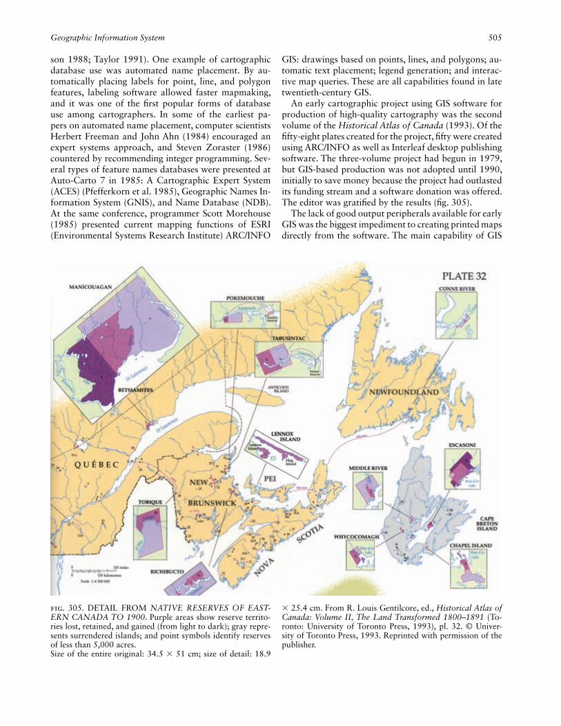
son 1988; Taylor 1991). One example of cartographic database use was automated name placement. By au-tomatically placing labels for point, line, and polygon features, labeling software allowed faster mapmaking, and it was one of the fi rst popular forms of database use among cartographers. In some of the earliest pa-pers on automated name placement, computer scientists Herbert Freeman and John Ahn (1984) encouraged an expert systems approach, and Steven Zoraster (1986) countered by recommending integer programming. Sev-eral types of feature names databases were presented at Auto-Carto 7 in 1985: A Cartographic Expert System (ACES) (Pfefferkorn et al. 1985), Geographic Names In-formation System (GNIS), and Name Database (NDB). At the same conference, programmer Scott Morehouse (1985) presented current mapping functions of ESRI (Environmental Systems Research Institute) ARC/INFO

GIS: drawings based on points, lines, and polygons; au-tomatic text placement; legend generation; and interac-tive map queries. These are all capabilities found in late twentieth-century GIS.

An early cartographic project using GIS software for production of high-quality cartography was the second volume of the Historical Atlas of Canada (1993). Of the fi fty-eight plates created for the project, fi fty were created using ARC/INFO as well as Interleaf desktop publishing software. The three-volume project had begun in 1979, but GIS-based production was not adopted until 1990, initially to save money because the project had outlasted its funding stream and a software donation was offered. The editor was gratifi ed by the results (fi g. 305).

The lack of good output peripherals available for early GIS was the biggest impediment to creating printed maps directly from the software. The main capability of GIS

Fig. 305. DETAIL FROM NATIVE RESERVES OF EAST-ERN CANADA TO 1900. Purple areas show reserve territo-ries lost, retained, and gained (from light to dark); gray repre-sents surrendered islands; and point symbols identify reserves of less than 5,000 acres.Size of the entire original: 34.5 × 51 cm; size of detail: 18.9

× 25.4 cm. From R. Louis Gentilcore, ed., Historical Atlas of Canada: Volume II, The Land Transformed 1800–1891 (To-ronto: University of Toronto Press, 1993), pl. 32. © Univer-sity of Toronto Press, 1993. Reprinted with permission of the publisher.

Geographic Information System 505

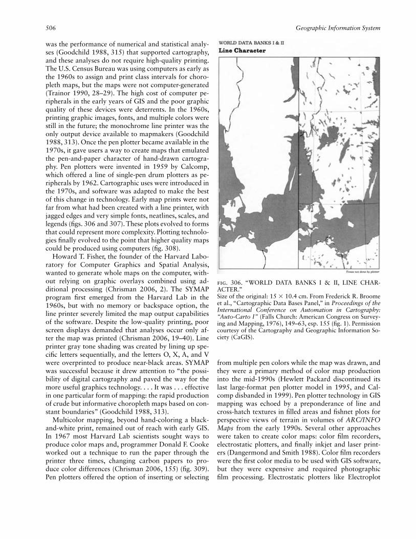
was the performance of numerical and statistical analy-ses (Goodchild 1988, 315) that supported cartography, and these analyses do not require high-quality printing. The U.S. Census Bureau was using computers as early as the 1960s to assign and print class intervals for choro-pleth maps, but the maps were not computer-generated (Trainor 1990, 28–29). The high cost of computer pe-ripherals in the early years of GIS and the poor graphic quality of these devices were deterrents. In the 1960s, printing graphic images, fonts, and multiple colors were still in the future; the monochrome line printer was the only output device available to mapmakers (Goodchild 1988, 313). Once the pen plotter became available in the 1970s, it gave users a way to create maps that emulated the pen-and-paper character of hand-drawn cartogra-phy. Pen plotters were invented in 1959 by Calcomp, which offered a line of single-pen drum plotters as pe-ripherals by 1962. Cartographic uses were introduced in the 1970s, and software was adapted to make the best of this change in technology. Early map prints were not far from what had been created with a line printer, with jagged edges and very simple fonts, neatlines, scales, and legends (fi gs. 306 and 307). These plots evolved to forms that could represent more complexity. Plotting technolo-gies fi nally evolved to the point that higher quality maps could be produced using computers (fi g. 308).

Howard T. Fisher, the founder of the Harvard Labo-ratory for Computer Graphics and Spatial Analysis, wanted to generate whole maps on the computer, with-out relying on graphic overlays combined using ad-ditional processing (Chrisman 2006, 2). The SYMAP program fi rst emerged from the Harvard Lab in the 1960s, but with no memory or backspace option, the line printer severely limited the map output capabilities of the software. Despite the low-quality printing, poor screen displays demanded that analyses occur only af-ter the map was printed (Chrisman 2006, 19–40). Line printer gray tone shading was created by lining up spe-cifi c letters sequentially, and the letters O, X, A, and V were overprinted to produce near-black areas. SYMAP was successful because it drew attention to “the possi-bility of digital cartography and paved the way for the more useful graphics technology. . . . It was . . . effective in one particular form of mapping: the rapid production of crude but informative choropleth maps based on con-stant boundaries” (Goodchild 1988, 313).

Multicolor mapping, beyond hand-coloring a black-and-white print, remained out of reach with early GIS. In 1967 most Harvard Lab scientists sought ways to produce color maps and, programmer Donald F. Cooke worked out a technique to run the paper through the printer three times, changing carbon papers to pro-duce color differences (Chrisman 2006, 155) (fi g. 309). Pen plotters offered the option of inserting or selecting

from multiple pen colors while the map was drawn, and they were a primary method of color map production into the mid-1990s (Hewlett Packard discontinued its last large-format pen plotter model in 1995, and Cal-comp disbanded in 1999). Pen plotter technology in GIS mapping was echoed by a preponderance of line and cross-hatch textures in fi lled areas and fi shnet plots for perspective views of terrain in volumes of ARC/INFO Maps from the early 1990s. Several other approaches were taken to create color maps: color fi lm recorders, electrostatic plotters, and fi nally inkjet and laser print-ers (Dangermond and Smith 1988). Color fi lm recorders were the fi rst color media to be used with GIS software, but they were expensive and required photographic fi lm processing. Electrostatic plotters like Electroplot

Fig. 306. “WORLD DATA BANKS I & II, LINE CHAR -ACTER.”Size of the original: 15 × 10.4 cm. From Frederick R. Broome et al., “Cartographic Data Bases Panel,” in Proceedings of the International Conference on Automation in Cartography: “Auto-Carto I” (Falls Church: American Congress on Survey-ing and Mapping, 1976), 149–63, esp. 155 (fi g. 1). Permission courtesy of the Cartography and Geographic Information So-ciety (CaGIS).

506 Geographic Information System

soon followed. By 1987, maps and other graphic prod-ucts could be directed to what Hugh W. Calkins and Duane F. Marble (1987, 109) considered fast and so-phisticated color printers. Laser and inkjet printers were commonplace by the end of the twentieth century, both providing high-quality map printing to a wide range of paper sizes.

Although GIS historically has lacked cartographic ele-ments, computer-assisted cartography systems also relied heavily on geographically referenced data. Computer-assisted cartography systems provided users with im-proved graphics, editing, and the capability of plotting their data (Tomlinson 1988, 258–59; Coppock 1988). The most popular of these computer-assisted cartogra-phy systems were variously called automated cartogra-phy, computer-mapping systems, and computer-aided design (CAD). Taylor (1974, 35) defi ned automated car-tography as automation of mapmaking processes. The maps that were produced with automated cartography were intended to resemble existing printed maps. In Can-ada in the early 1970s, automated cartography software was used to replicate topographic and marine charts. In contrast, Taylor defi ned computer mapping as map pro-duction using the analytical power of computers. The maps produced from computer mapping software were different from those of an automated cartography sys-tem in that they were designed to be the rough prod-ucts from a GIS rather than high-quality cartography for commercial distribution. CAD, which continued to be used for mapping through the 1990s, did not provide users with the database capabilities of GIS, but did pro-vide detailed and accurate graphics (Pratt 1985). David Rhind (1988, 286) argued that, as a spin-off from GIS, computer-assisted cartography systems were unlikely to be viable economically. By the end of the twentieth cen-tury the systems had nearly disappeared, but they were considered distinct from GIS at the height of their use.

The early inventories of software functions by GIS World also attempted to divide systems into types. The 1989 survey used seven categories: GIS, automated mapping, desktop mapping, facilities management, im-age processing, computer-assisted design, and computer- assisted engineering, with some companies selecting three or four of these choices to describe their systems. This partitioning seems quite detailed, but market sectors were being established and they could be contentious. For ex-ample, GIS World (Anonymous 1989, 11) reports that Daratech’s study, GIS Markets and Opportunities, was criticized for concluding that Intergraph controlled 49.9 percent of the GIS market worldwide because the study defi ned the subject broadly to include hundreds of auto-mated mapping systems not considered to be “true GIS.”

Lesser-known computer-assisted cartography systems also relied on geographically referenced data. Electronic mapping systems (EMS) produced maps used in elec-tronic media such as the electronic atlas and included functionality similar to GIS along with good cartographic display (Taylor 1991, 6). The digital cartographic data-base described by Calkins and Marble (1987) ran much like GIS in that its associated database contained infor-mation about the map and provided greater fl exibility

Fig. 307. SYMBOLS AND SAMPLE TYPE.Size of the original: 5.6 × 5.1 cm (top) and 10 × 8.9 cm (bot-tom). From Clyde G. Johnson, Allen V. Hershey, and Aubrey L. LeBlanc, “Cartographic Symbology Panel,” in Proceedings of the International Conference on Automation in Cartography: “Auto-Carto I” (Falls Church: American Congress on Survey-ing and Mapping, 1976), 215–39, esp. 223 and 224 (fi gs. 6 and 7). Permission courtesy of the Cartography and Geographic Information Society (CaGIS).

Geographic Information System 507

for the cartographic designer. Because many GIS spe-cialists did not have specifi c cartographic training, sev-eral systems were invented with the intention of having the system become the cartographer. One type of such computer-assisted cartographic systems was expert sys-tems or intelligent knowledge-based systems (Robinson and Jackson 1985). The Digital Cartography Program was developed in the mid-1980s at the USGS to produce maps from a GIS to increase production effi ciency. In one part of this program, base maps and other digital data were available to produce thematic maps quickly and easily once imported from a GIS (Southard and An-derson 1983).

Finally, the Digital Chart of the World (DCW), a small-scale vector data set developed by ESRI in the early 1990s for the U.S. Defense Mapping Agency, be-

came available on CD-ROM for anyone to use. While not a software program, the DCW (later called VMAP) did offer data digitized from more than 250 Operational Navigation Charts and Jet Navigation Charts from four different countries by the U.S. National Imagery and Mapping Agency (NIMA). The DCW was valuable be-cause it brought a great amount of data together in one place and was relatively easy to access. It also prompted consternation among European partners who accused the United States of data dumping—of freely distribut-ing what had been their intellectual property in a man-ner that undercut their cost recovery efforts through selling the same data (discussed at the International Car-tographic Association 15th Conference, Bournemouth, 1991).

Intermediate computer-assisted map production solu-

Fig. 308. OTTAWA-HULL (CENSUS TRACTS).Size of the original: 17.1 × 22.3 cm. From Thomas C. Waugh and D. R. F. Taylor, “GIMMS/An Example of an Operational

System for Computer Cartography,” Canadian Cartographer 13 (1976):158–66, fi g. 1 (between 162 and 163). Permission courtesy of D. R. F. Taylor, Carleton University, Ottawa.

508 Geographic Information System

tions were also common, such as printing separations by choropleth categories and combining these with tra-ditional manual production methods (see, for example, health atlas production as reviewed in Pickle 2009). An-other combination was to use GIS to plot boundary or contour lines and then copy them at reduced scale on photographic negatives to create fi ner lines. The nega-tives were then used to expose Peelcoat material and produce open-window negatives for color separated area fi lls. Judy M. Olson’s students at Michigan State University, University of Minnesota, and Boston Uni-versity experimented with these combinations of auto-mated and traditional methods, producing process-color printed, postcard-sized maps throughout the 1980s.

As graphic design software such as Aldus FreeHand and Adobe Illustrator developed more complete func-tions for editing lines, areas, and labels in the early 1990s, cartographers took advantage of GIS to prepare selected map elements using existing databases, such as projecting a coastline from digital data, exporting the lines, and continuing production in a graphics software environment that supported PostScript printing. These

exported maps from GIS were often mediated through early versions of the Adobe Illustrator format and out-put with dramatic color differences so they could be sep-arated into particular line styles with more nuanced dif-ferences using design tools such as variable line weights and dashing. This meant that unfi nished GIS maps were garish before export and completed in a graphics soft-ware environment. This combination also allowed the use of service bureaus with imagesetters that produced professional quality fi lm negatives at 12,000 dots per inch and higher. These dot densities are needed to pro-duce halftone screens required for creating a full color gamut from process color ink combinations used in tra-ditional high-quality lithographic printing.

M. J. Blakemore (1985), in his short history of digital mapping from line printer maps to GIS, says that the emergence of digital mapping established a long period of aggravation among cartographic specialists. Byron Moldofsky (personal communication, 9 February 2011) refl ects on GIS-based production of plates for volume 2 of the Historical Atlas of Canada as an intricate process requiring separate EPS (encapsulated PostScript) fi les for maps, other graphics, and English and French labeling and text layers, which were sent to a service bureau on fl oppy disks where they were recombined to make nega-tives, proofs, and eventually plates. Likewise, Bickmore predicted that just as bad programmers waste com-puter time, poor information handling would hamper automated cartography if expertise were not improved in this new domain. The cartographic conversations at academic conferences at the end of the century were rife with hand wringing about bad maps wrought with GIS, but there are numerous examples of reasonably profes-sional mapping on a wide range of topics displayed in annual volumes of the ESRI Map Book (initially titled ARC/INFO Maps in 1984). For example, volume 15, published in 2000, presents 111 map projects, including hillshading and hypsometric tints, proportioned traffi c fl ows, bike routes, 3-D buildings, one- and two-variable choropleth maps, soil and geology classifi cations, land cover distributions, environmental risks, orthophoto and vector map combinations, cadastral maps, infrastructure detail, and political boundaries, to name a subset. This series also provides ways to look back on GIS mapping: volume 25 of the ESRI Map Book (2010) presents four pairs of maps by the same agencies, contrasting rough black-and-white line maps from the fi rst map books with modern full-color high-resolution products to show the evolution of GIS as a tool for map production. The map authors may have been aggravated or wasted their time in the course of map production, but they were certainly doing publishable cartography using GIS by the end of the twentieth century.

Carolyn Fish and Cynthia A. Brewer

Fig. 309. COLORED SYMAP OUTPUT. New Haven, Con-necticut, population density by census blocks from 1967 test census.Image courtesy of Esri, Redlands. Permission courtesy of URISA, Des Plaines.

Geographic Information System 509

See also: Electronic Cartography: (1) Data Capture and Data Conver-sion, (2) Display Hardware; Experimental Cartography Unit, Royal College of Art (U.K.); Harvard Laboratory for Computer Graphics and Spatial Analysis (U.S.); SYMAP (software)

Bibliography:Anonymous. 1988. “1988 GIS Software Survey.” GIS World 1,

no. 1:7–11.———. 1989. “Daratech Study Draws Praise, Fire.” GIS World 2,

no. 5:11.Blakemore, M. J. 1985. “From Lineprinter Maps to Geographic Infor-

mation Systems: A Retrospective on Digital Mapping.” Bulletin of the Society of University Cartographers 19:65–70.

Borgerding, L. H., F. E. Lortz, and J. K. Powell. 1983. “Computer-Assisted Map Compilation, Editing, and Finishing.” In Auto-Carto 5 Proceedings: Environmental Assessment and Resource Manage-ment, ed. Jack Foreman, 141–46. Falls Church: American Society of Photogrammetry and American Congress on Surveying and Map-ping.

Brewer, Cynthia A., and Trudy A. Suchan. 2001. Mapping Census 2000: The Geography of U.S. Diversity. Washington, D.C.: U.S. De-partment of Commerce, Economics and Statistics Administration, U.S. Census Bureau.

Calkins, Hugh W., and Duane F. Marble. 1987. “The Transition to Automated Production Cartography: Design of the Master Carto-graphic Database.” American Cartographer 14:105–19.

Chrisman, Nicholas R. 2006. Charting the Unknown: How Computer Mapping at Harvard Became GIS. Redlands: ESRI Press.

Coppock, J. T. 1988. “The Analogue to Digital Revolution: A View from an Unreconstructed Geographer.” American Cartographer 15:263–75.

Dangermond, Jack, and Lowell Kent Smith. 1988. “Geographic Infor-mation Systems and the Revolution in Cartography: The Nature of the Role Played by a Commercial Organization.” American Cartog-rapher 15:301–10.

Freeman, Herbert, and John Ahn. 1984. “AUTONAP—an Expert Sys-tem for Automatic Map Name Placement.” In Proceedings of the International Symposium on Spatial Data Handling, 2 vols., 1:544–69. Zurich: Geographisches Institut, Abteilung Kartographie/EDV, Universität Zürich-Irchel.

GIS World, Inc. 1989. The GIS Sourcebook. Fort Collins: GIS World.Goodchild, Michael F. 1988. “Stepping Over the Line: Technological

Constraints and the New Cartography.” American Cartographer 15:311–19.

Keller, C. Peter, and Nigel M. Waters. 1991. “Mapping Software for Microcomputers.” In Geographic Information Systems: The Micro-computer and Modern Cartography, ed. D. R. F. Taylor, 97–128. Oxford: Pergamon Press.

Morehouse, Scott. 1985. “ARC/INFO: A Geo-Relational Model for Spatial Information.” In Auto-Carto 7 Proceedings: Digital Repre-sentations of Spatial Knowledge, 388–97. Falls Church: American Society of Photogrammetry and American Congress on Surveying and Mapping.

Pfefferkorn, C., et al. 1985. “ACES: A Cartographic Expert System.” In Auto-Carto 7 Proceedings: Digital Representations of Spatial Knowledge, 399–407. Falls Church: American Society of Photo-grammetry and American Congress on Surveying and Mapping.

Pickle, Linda Williams. 2009. “A History and Critique of U.S. Mortal-ity Atlases.” Spatial and Spatio-Temporal Epidemiology 1:3–17.

Pratt, Stephen H. 1985. “A Non-problematic Approach to Cartogra-phy within the Constructs of a Geographic Information System” (abstract). In Auto-Carto 7 Proceedings: Digital Representations of Spatial Knowledge, 416. Falls Church: American Society of Photo-grammetry and American Congress on Surveying and Mapping.

Rhind, David. 1988. “Personality as a Factor in the Development of a Discipline: The Example of Computer-Assisted Cartography.” American Cartographer 15:277–89.

Robinson, Gary, and Michael Jackson. 1985. “Expert Systems in Map Design.” Auto-Carto 7 Proceedings: Digital Representations of Spa-tial Knowledge, 430–39. Falls Church: American Society of Photo-grammetry and American Congress on Surveying and Mapping.

Southard, R. B., and K. E. Anderson. 1983. “A National Program for Digital Cartography.” In Auto-Carto 5 Proceedings: Environmental Assessment and Resource Management, ed. Jack Foreman, 41–49. Falls Church: American Society of Photogrammetry and American Congress on Surveying and Mapping.

Taylor, D. R. F. 1974. “The Canadian Cartographer and the Computer/Present Trends and Future Challenges.” Canadian Cartographer 11:35–44.

———. 1991. “Geographic Information Systems: The Microcomputer and Modern Cartography.” In Geographic Information Systems: The Microcomputer and Modern Cartography, ed. D. R. F. Taylor, 1–20. Oxford: Pergamon Press.

Tomlinson, Roger F. 1988. “The Impact of the Transition from Ana-logue to Digital Cartographic Representation.” American Cartog-rapher 15:249–61.

Trainor, Timothy F. 1990. “Fully Automated Cartography: A Major Transition at the Census Bureau.” Cartography and Geographic In-formation Systems 17:27–38.

Zoraster, Steven. 1986. “Integer Programming Applied to the Map La-bel Placement Problem.” Cartographica 23, no. 3:16–27.

Metadata. As “data about data,” metadata are the equi-valent of a library’s card catalog. Metadata allow a pro-ducer to advertise data and provide a user with infor-mation to make a decision about whether the data are appropriate for an application. Today metadata typically are stored as an XML (extensible markup language) fi le that is easily found and harvested with standard internet tools.

Metadata include information about data or geospa-tial services, such as content, source, vintage, spatial scale, accuracy, projection, responsible party, contact phone number, method of collection, and other descrip-tors. Metadata are critical to document, preserve, and protect spatial data assets. Reliable metadata, structured in a standardized manner, are essential to ensuring that geospatial data are used appropriately and that any re-sulting analysis is credible.

In order to bring geospatial data producers and con-sumers together the Federal Geographic Data Commit-tee (FGDC) placed a high priority on creating a useful and rigorous metadata standard. The formalization of this standard began with an executive order by Presi-dent Bill Clinton in 1994 that formally established the National Spatial Data Infrastructure (NSDI). It referred to “Standardized Documentation of Data” and ex-pressed some urgency: “Beginning 9 months from the date of this order, each agency shall document all new geospatial data it collects or produces, either directly or indirectly, using the standard under development by the FGDC, and make that standardized documentation electronically accessible to the Clearinghouse network” (U.S. President 1994, 17,672).

The FGDC established the fi rst content standard for digital geospatial metadata in 1994 and revised the

510 Geographic Information System

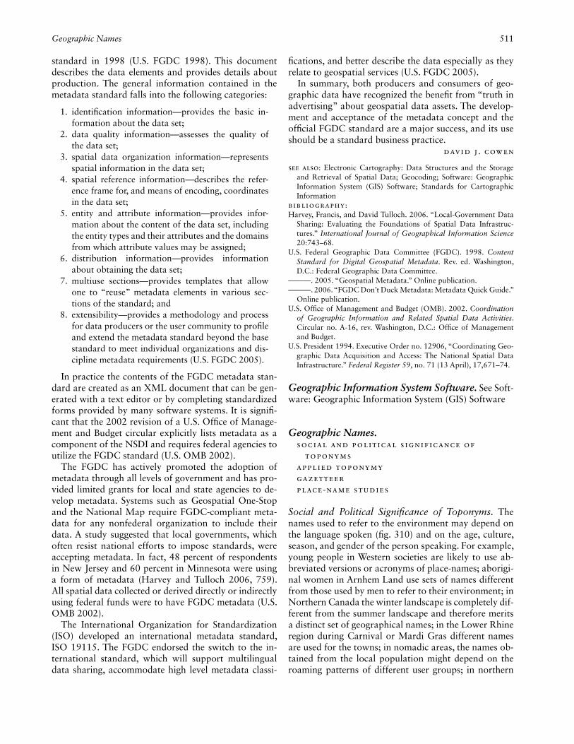
Geographic Names 511

standard in 1998 (U.S. FGDC 1998). This document describes the data elements and provides details about production. The general information contained in the metadata standard falls into the following categories:

1. identifi cation information—provides the basic in-formation about the data set;

2. data quality information—assesses the quality of the data set;

3. spatial data organization information—represents spatial information in the data set;

4. spatial reference information—describes the refer-ence frame for, and means of encoding, coordinates in the data set;

5. entity and attribute information—provides infor-mation about the content of the data set, including the entity types and their attributes and the domains from which attribute values may be assigned;

6. distribution information—provides information about obtaining the data set;

7. multiuse sections—provides templates that allow one to “reuse” metadata elements in various sec-tions of the standard; and

8. extensibility—provides a methodology and process for data producers or the user community to profi le and extend the metadata standard beyond the base standard to meet individual organizations and dis-cipline metadata requirements (U.S. FGDC 2005).

In practice the contents of the FGDC metadata stan-dard are created as an XML document that can be gen-erated with a text editor or by completing standardized forms provided by many software systems. It is signifi -cant that the 2002 revision of a U.S. Offi ce of Manage-ment and Budget circular explicitly lists metadata as a component of the NSDI and requires federal agencies to utilize the FGDC standard (U.S. OMB 2002).

The FGDC has actively promoted the adoption of metadata through all levels of government and has pro-vided limited grants for local and state agencies to de-velop metadata. Systems such as Geospatial One-Stop and the National Map require FGDC-compliant meta-data for any nonfederal organization to include their data. A study suggested that local governments, which often resist national efforts to impose standards, were accepting metadata. In fact, 48 percent of respondents in New Jersey and 60 percent in Minnesota were using a form of metadata (Harvey and Tulloch 2006, 759). All spatial data collected or derived directly or indirectly using federal funds were to have FGDC metadata (U.S. OMB 2002).

The International Organization for Standardization (ISO) developed an international metadata standard, ISO 19115. The FGDC endorsed the switch to the in-ternational standard, which will support multilingual data sharing, accommodate high level metadata classi-

fi cations, and better describe the data especially as they relate to geospatial services (U.S. FGDC 2005).

In summary, both producers and consumers of geo-graphic data have recognized the benefi t from “truth in advertising” about geospatial data assets. The develop-ment and acceptance of the metadata concept and the offi cial FGDC standard are a major success, and its use should be a standard business practice.

David J. Cowen

See also: Electronic Cartography: Data Structures and the Storage and Retrieval of Spatial Data; Geocoding; Software: Geographic Information System (GIS) Software; Standards for Cartographic Information

Bibliography:Harvey, Francis, and David Tulloch. 2006. “Local-Government Data

Sharing: Evaluating the Foundations of Spatial Data Infrastruc-tures.” International Journal of Geographical Information Science 20:743–68.

U.S. Federal Geographic Data Committee (FGDC). 1998. Content Standard for Digital Geospatial Metadata. Rev. ed. Washington, D.C.: Federal Geographic Data Committee.

———. 2005. “Geospatial Metadata.” Online publication.———. 2006. “FGDC Don’t Duck Metadata: Metadata Quick Guide.”

Online publication.U.S. Offi ce of Management and Budget (OMB). 2002. Coordination

of Geographic Information and Related Spatial Data Activities. Circular no. A-16, rev. Washington, D.C.: Offi ce of Management and Budget.

U.S. President 1994. Executive Order no. 12906, “Coordinating Geo-graphic Data Acquisition and Access: The National Spatial Data Infrastructure.” Federal Register 59, no. 71 (13 April), 17,671–74.

Geographic Information System Software. See Soft-ware: Geographic Information System (GIS) Software

Geographic Names.Social and Political Significance of

ToponymsApplied ToponymyGazetteerPlace-Name Studies

Social and Political Signifi cance of Toponyms. The names used to refer to the environment may depend on the language spoken (fi g. 310) and on the age, culture, season, and gender of the person speaking. For example, young people in Western societies are likely to use ab-breviated versions or acronyms of place-names; aborigi-nal women in Arnhem Land use sets of names different from those used by men to refer to their environment; in Northern Canada the winter landscape is completely dif-ferent from the summer landscape and therefore merits a distinct set of geographical names; in the Lower Rhine region during Carnival or Mardi Gras different names are used for the towns; in nomadic areas, the names ob-tained from the local population might depend on the roaming patterns of different user groups; in northern

512 Geographic Names

Norway. Norse farmers and Saami (Sami; Lapp) nomads refer differently to aspects of the same environment, as is visible on Norwegian topographic maps, where sometimes name pairs occur (for mountains and slopes only Saami names may be known, while infrastructural works almost always bear Norwegian names); on Java, different sets of names relating to the environment are used when speaking to someone perceived to be on a higher social level than when speaking to someone on a lower social level.

It is not clear when it was fi rst realized that geograph-ical names were also carriers of meaning not in the ety-mological sense or in the sense of signposts or labels for orientation but in the sense that a geographical fea-ture named in a specifi c language could be a manifes-tation of the fact that the area belonged to the people speaking that language. Based on the ideas of national-ism, the thinking was that if people are speaking one language they must belong to one group so their area should be united, and conversely, if a region is to be a part of one nation the names in that region must refl ect this belonging, requiring current names to be changed. For example, as a tribute for the help provided by Na-poleon III, Savoia and Nizza were transferred to France after the Italian unifi cation. This transfer was followed by the Frenchifi cation of the Italian geographical names in the areas: hence Savoie and Nice.

This practice was followed to the fullest in Europe between 1870 and 1970. Two examples in 1918 were the Italianization of the South Tyrolean place-names by Ettore Tolomei and the reversion to the former French-ifi ed place-names for the Alsace. Between the two world wars there was the Germanization of place-names with

Slavonic roots in Eastern Germany, and after World War II there was the Polonization of German place-names in the parts of pre-1937 Germany occupied by Poland after 1945. Under Nicolae Ceausescu in Roma-nia, Hungarian and German village names were obliter-ated by razing the villages and concentrating the rural population in new towns with Romanian names. At the end of the century this practice could still be seen in Ko-sovo and Bosnia, where toponymic cleansing went hand in hand with ethnic cleansing.

During the twentieth century a change in the political attitudes toward minority populations residing in a na-tion also can be seen in toponymic changes. Whereas in the nineteenth century, British politicians stated openly in parliament that if the Welsh needed maps with their own place-names, they should produce them themselves (conveniently forgetting that the Welsh were paying taxes and thus had an equal right to the preservation of their cultural heritage), the twentieth century saw the development by the Ordnance Survey of special guidelines for topographers on how to render Gaelic and Welsh names correctly (Harley 1971). In Spain af-ter the victory of General Francisco Franco all manifes-tations of regionalism were rigidly obliterated. It was only after 1980 that regional autonomy in Catalonia, the Basque Provinces, and Galicia were reinstituted, and place-names reverted from their Castilian version back to their Catalan, Basque, or Galician versions: Gerona became Girona, San Sebastián became Donostia, and La Coruña became A Coruña. In Scandinavia, Norway, Sweden, and Finland worked together in standardizing the rendering of the various Saami languages on their maps. On French topographic maps features might be rendered bilingually, with Catalan or Breton names next to the French versions. In the Netherlands until 1980 topographers translated place-names in the Frisian lan-guage minority area into Dutch. This practice was dis-continued and monolingual rendering of Frisian place-names became an option. Even the name of the province Frisia was offi cially codifi ed into Fryslân. In Germany the positive discrimination of Sorbian place-names in Lusatia, understandable when the German Democratic Republic was part of the predominantly Slavonic Soviet Bloc, was continued after reunifi cation (fi g. 311). So gen-erally speaking, all through Western Europe geographi-cal names from autochthonous linguistic minority areas increasingly have tended to be recognized and accepted.

A similar twentieth-century change is recognized in the reuse of aboriginal or native names in areas of Australia and the Americas. The sixteenth through nineteenth cen-tury expansion of European infl uence over the Americas and Australia brought with it a submergence of native names. When one compares an overview map of the Midwestern United States from 1784 to one from 1872

Fig. 310. NORWEGIAN, NORTHERN SAAMI, AND KVÆNER PLACE-NAMES FOR THE SAME PLACE IN NORTHERN NORWAY.Image courtesy of Nils Øivind Helander.

Geographic Names 513

the percentage of native names falls from 80 percent to a mere 10 percent (fi gs. 312 and 313). Native names, if kept by the settlers, were often modifi ed, distorted, and codifi ed. By the end of the twentieth century there were movements among the descendants of the original populations to restore the original names. This collided with two other forces: (1) to keep things as they are—major cities like Chicago or Ottawa did not change the spelling of their names because of modifi cations made by the Western European settlers, and (2) a fear that rec-ognition and restoration of a native name might have connotations of native title to the land. The Wik case in

Queensland, Australia, serves as a good example (Bren-nan 1998).

Political “cults of personality” led to toponymic changes in the twentieth century. Communism, and to a lesser degree Nazism, tended to glorify its revolution-ary heroes by bestowing their names on existing places. The best-known Communist examples are Leningrad for Sankt-Peterburg and Karl-Marx-Stadt for Chemnitz in Germany. Hundreds of geographical features were (re)named after Joseph Stalin, from Stalingrad (formerly Tsaritsyn, now Volgograd) to Stalin Peak or Pik Stalina (named 1933, changed in 1962 to Communism Peak or Pik Kommunizma and in 1998 to Ismail Samani Peak [in Tajik: Qullai Ismoili Somoni]). Under Nikita Khru-shchev, a de-Stalinization campaign changed most of them back. After 1990 almost all Communist-imposed names reverted to their pre-1917 versions, with the ex-ception of Kaliningrad for the former German Königs-berg. Mikhail Kalinin, head of state of the Soviet Union 1922–46 also had Kalinin (now reverted to Tver) and a second Kaliningrad, near Moscow (previously Podlipki, but renamed Korolev after a spacecraft engineer), was named after him.

Toponymic change was also used to support war pro-paganda. One of the results of World War I was that place-names given by German settlers in the United States, Canada, and Australia were changed into English place-names. The example given here is taken from South Australia. The “Nomenclature Committee’s Report on Enemy Place Names” (in the Proceedings of the Parlia-ment of South Australia, 1916), based on a resolution in the South Australian Assembly, stated that “the names of all towns and districts in South Australia which indicate a foreign enemy origin should be altered.” A proposal followed to change sixty-nine place-names of German origin. This was gazetted in 1918. For example, Rhine River North changed to The Somme, Rhine River South to The Marne, Rhine Villa to Cambrai, Kaiserstuhl to Mount Kitchener, and Grunthal to Verdun. Klemzig was changed into Gaza, but later, in 1935, reverted again, as did Hahndorf, which was named Ambleside from 1918–35.

In colonial areas that became independent during the twentieth century there have been movements to rid the land of names that were considered linked to the colo-nial infrastructure. Africa poses many examples: Lou-renço Marques to Maputo, Fort-Lamy to N’Djamena, Salisbury to Harare, Léopoldville to Kinshasa. This also happened in other areas where the majority thought the names used should refl ect the majority language groups instead of historical reality: an example was the change of Pretoria to Tshwane. Sometimes the leaders of newly independent states used their own names. Examples were Lake Albert and Lake Edward, which changed into Lake

Fig. 311. MAP KEY FROM A BILINGUAL TOWN PLAN. From the Stadtplan Bautzen Budyšin, a Sorb-speaking area in Lusatia, former East Germany, 1986.Size of the original map key: 18.2 × 10 cm.

514 Geographic Names

Mobutu Sese Seko and Lake Idi Amin Dada (and have since changed back). As discomfort with these leaders followed their loss of power, the previous names seem to have reestablished themselves. Only Lake Victoria ap-parently survived this decolonization trend. Similarly, in India the major changes of Bombay to Mumbai and Madras to Chennai can be classed as the deposition of colonial names.

At the end of the twentieth century there remain to-ponymic issues. The Turkish occupation of Northern Cyprus and the ensuing obliteration of the Greek place-names resulted in the United Nations Group of Experts on Geographical Names (UNGEGN) drafting a resolu-tion at the Third UN Conference on the Standardization of Geographical Names in Athens, 1977, that stated, “It is recommended that any changes made by other authorities in the names standardized by a competent national geographical names authority should not be

recognized by the United Nations” (Resolution III-16). The name Persian Gulf was almost universally accepted in the seventeenth century. It was named as the Gulf of al-Qatif on some charts until the new economic rise of the Arab states bordering on the Persian Gulf caused them to claim the name Arabian Gulf (this name also has been used as an alternative for the name Red Sea in the past). Iran requested UNGEGN to safeguard its cultural heritage by protecting the Persian names of the islands in the Persian Gulf.

The name for the body of water between Korea and Japan was called Sea of Korea or East Sea in the six-teenth to eighteenth century, but by the end of the nine-teenth century the name Sea of Japan was widely used, even before Japan turned Korea into a protectorate in 1905 and in 1910 annexed it. In 1928 Japan had the name Sea of Japan incorporated in the International Hydrographic Organization’s Limits of Oceans and

Fig. 312. DETAIL FROM A NEW AND CORRECT MAP OF THE UNITED STATES OF NORTH AMERICA, 1784, BY ABEL BUELL. This portion of the North American Mid-west on Buell’s map used mostly indigenous names; compare fi gure 313.

Size of the entire original: 127 × 160 cm; size of detail: ca. 42 × 60 cm. British Library, London (Maps *71490.[150]). © The British Library Board, all rights reserved 03/01/15.

Geographic Names 515

Seas. Both the Republic of Korea and the Democratic Republic of Korea at the end of the twentieth century claimed that the sea should be given the more neutral name of East Sea. When the southernmost federal state in Yugoslavia was called Macedonia, the Greeks did not object, but when this state became an independent na-tion in 1991, Greece objected to this name as its use would lay a claim on the adjacent Greek province of Macedonia. Pending this name dispute with Greece, the country was admitted in 1993 to the United Nations under the provisional reference “The Former Yugoslav Republic of Macedonia” (FYROM) (Monmonier 2006, 100–101). Fortunately, the UNGEGN, while never mak-ing decisions on individual names, is in place to create and suggest the use of toponymic principles in order to

solve such issues. Even so, the naming of a number of countries or bodies of water is still being contested in UNGEGN discussions.

Ferjan Ormeling

See also: Board on Geographic Names (U.S.); Geopolitics and Car-tography; Indigenous Peoples and Western Cartography; Permanent Committee on Geographical Names (U.K.); United Nations

Bibliography:Andrews, J. H. 2002. A Paper Landscape: The Ordnance Survey in

Nineteenth-Century Ireland. 2d ed. Dublin: Four Courts Press.Aurousseau, Marcel. 1957. The Rendering of Geographical Names.

London: Hutchinson University Library.Belen’kaya, V. D. 1975. “Current Tendencies in the Naming of Places.”

Soviet Geography 16:315–20.Brennan, Frank. 1998. The Wik Debate: Its Impact on Aborigines,

Pastoralists and Miners. Sydney: UNSW Press.

Fig. 313. DETAIL FROM THE AMERICAN UNION RAIL-ROAD MAP OF THE UNITED STATES, BRITISH POS-SESSIONS, WEST INDIES, MEXICO, AND CENTRAL AMERICA, 1871. The Midwest portion contains mostly Eu-ropean names; compare fi gure 312.

Size of the entire original: 95 × 132 cm; size of detail: ca. 18.5 × 26.7 cm. Image courtesy of the David Rumsey Map Collection.

516 Geographic Names

Canadian Permanent Committee on Geographical Names. 1992. Guide to the Field Collection of Native Geographical Names. Ot-tawa: Energy, Mines and Resources Canada, Surveys, Mapping and Remote Sensing Sector.

Deslandes, Gaston. 1947. “La doctrine toponymique de l’I.G.N. et son application cartographique.” Onomastica 1:322–28.

Harley, J. B. 1971. “Place-Names on the Early Ordnance Survey Maps of England and Wales.” Cartographic Journal 8:91–104.

Kadmon, Naftali. 2000. Toponymy: The Lore, Laws and Language of Geographical Names. New York: Vantage Press.

Kirrinnis, Herbert. 1942. “Die Ortsnamenänderungen in Ostpreußen.” Petermanns Geographische Mitteilungen 88:265–70.

Monmonier, Mark. 2006. From Squaw Tit to Whorehouse Meadow: How Maps Name, Claim, and Infl ame. Chicago: University of Chi-cago Press.

Ormeling, Ferdinand J. 1980. “Exonyms: An Obstacle to International Communication.” ITC Journal 1980-1:162–76.

Ormeling, Ferjan. 1983. Minority Toponyms on Maps: The Rendering of Linguistic Minority Toponyms on Topographic Maps of Western Europe. Utrecht: Depart. of Geography, University of Utrecht.

Tolomei, Ettore, Ettore De Toni, and Vittorio Emanuele Baroncelli. 1916. Prontuario dei nomi locali dell’Alto Adige. Rome: Reale So-cietà Geografi ca Italiana.

Applied Toponymy. Geographic names are necessary for spatial reference in an otherwise confusing land-scape. Names are applied to landmarks in the develop-ment of our sense of place and become the means by which we describe the landscape. Generally, names refer to specifi c features, and this conveys information about how people categorize spatial phenomena. Geographic names are initially connotative, but in the course of their development and use become denotative—that is, labels that serve as referents to specifi c landmarks.

In the naming process, those proposing a name are almost always aware of the meaning of the name (con-notative) as well as the reasons for its application. How-ever, reasons often are known only locally; with usage and time they may become muddled or forgotten. The name becomes merely a label (denotative) and does not depend on context for functionality. The activities of specifi c reference and categorization may become quite complex, employing highly variable, personal, and often idiosyncratic methods of perception. Standardization of geographic names is therefore essential for emergency preparedness, regional and local planning, site selection and analysis, environmental problem-solving, carto-graphic application, and all levels of communication.

Since names identify landmarks, and since maps, whether conventional or digital, abstractly represent as-pects and themes of the spatial environment, the use of geographic names is critical in even the most elementary use of any map. Meredith F. “Pete” Burrill (1990), execu-tive secretary emeritus of the U.S. Board on Geographic Names and cofounder of the United Nations Group of Experts on Geographical Names (UNGEGN), often stated that names are the language of maps. The appli-cation of geographic names is an integral part of the

cartographic process, which is evident in every national mapping program as well as in the numerous special-ized and general cartographic applications throughout government and the private sector.

The use of geographic names is not limited to car-tography but is inextricably part of other applications ranging from postal and delivery services to boundary defi nitions to genealogy. Applied toponymy is the recog-nition and use of geographic names as a specifi c element necessary to provide solutions to real-world problems. A basic element of applied toponymy is the standardized toponym or geographic name. Major projects, includ-ing cartographic ones, often are delayed, and even post-poned, until the geographic names are correct.

Applied toponymy is not new, but the term and its recognition conceptually as a means of assisting in solv-ing problems has gained wide attention and recognition only in the last decade of the twentieth century. This is partly a result of the rapid development and increased use of geographic information systems (GIS). As a tool for searching and retrieving information on the Internet and in data mining and linking seemingly disparate top-ics and categories, the use of geographic names or ap-plied toponymy is essential.

In concert with the development of printing, techni-cal advancements in mapmaking grew steadily from the sixteenth through the nineteenth centuries. Exploration and military campaigns increased and expanded the use of maps. As mapmaking techniques and the use of maps proliferated so did confusion in the use and applica-tion of geographic names. There was little or no com-munication or discussion among explorers, soldiers, and cartographers from one nation to another. Names were assigned as needed, and this led to different geographic names being used for the same feature.

The nineteenth century was a time of rapid devel-opment in modes of travel. One of the fi rst organized references to the problem of the use of nonstandard geographic names came at the fi rst meeting of the In-ternational Geographical Congress in Antwerp in 1871. Delegates called for the standardization of place-names on maps. In 1875, the Universal Postal Union declared it necessary to establish standard names of countries, cit-ies, and towns for purposes of effi cient delivery of the mail. During the 1890s, the fi rst committees were es-tablished to standardize the form and orthography of geographic names.

After the American Civil War, there were numerous government-sponsored scientifi c expeditions to the Western United States. These expeditions yielded new information and fairly accurate maps of some areas. However, each expedition needed names on its maps as referents for features on the landscape, and frequently geographic names were applied without any thought of

Geographic Names 517

potential confusion, thereby rendering some maps al-most useless. As a remedy, on 4 September 1890 U.S. President Benjamin Harrison issued an executive order creating a committee to establish principles, policies, and procedures for standardizing geographic names. The committee was given the authority to adjudicate controversies, and its decisions were fi nal. This mile-stone in the history of the standardization of geographic names and applied toponymy was to provide “uniform usage in regard to geographic nomenclature and orthog-raphy . . . throughout the Executive Departments of the Government” (Harrison 1890). Canada and the United Kingdom soon followed with similar committees, and by the fi rst decade of the twentieth century the beginnings of the systematic standardization of geographic names had begun. In 1947, the committee was abolished and reestablished (U.S. Congress 1947).

The growing number of names resulting from expan-sion and settlement during the eighteenth and nine-teenth centuries and the growing need and resultant increase in accuracy of record keeping made gazetteers and geographic indexes an expedient means of identify-ing places, features, and areas. National gazetteers were published in the late nineteenth century and throughout most of the twentieth century, but these often included only cities and large natural features. The goal of com-pleteness, although desired, was generally recognized as impractical, even impossible, given the ever increasing number of names.

The magnitude of the geographic names problem be-came apparent internationally as the number of issues continued to grow throughout the two world wars of the fi rst half of the twentieth century. The issues were apparent even within countries where attempts at stan-dardization had been established. Cartographers became directly involved in 1909, when the International Car-tographic Committee called on its members to address the issue of geographic names on maps. In 1919, the International Hydrographic Conference issued a similar statement regarding chartmaking. By the 1950s, numer-ous international organizations had issued statements calling for resolution of the growing and somewhat dan-gerous problem of the lack of standardized name usage. The newly created United Nations began to receive and record various inquiries and suggestions regarding the problem.

On 23 April 1959, the United Nations established a group of experts representing a cross-section of the in-ternational community dealing with geographic names to examine the problems and make recommendations. The group (later formally UNGEGN) met in June and July 1960 to consider the technical problems of domes-tic standardization of geographic names. It is most im-portant to note that the group of experts never consid-

ered as an option the establishment of an international body for adjudicating controversies and problems. Such an international body would not be able to deal with the varying requirements of countries. It is the inherent right of individual countries to solve their own topo-nymic problems. The 1960 meetings recommended the systematic national collection of geographic names, the establishment of offi ce procedures for offi cial treatment of geographic names, and a program of promulgation in each nation.

The meeting also stated the desirability of holding an international conference on the subject. The fi rst United Nations Conference on the Standardization of Geographical Names was held in September 1967 in Geneva. Resolution 4 urged all member nations to es-tablish a national names authority for the purpose of developing a program for standardizing geographic names (United Nations 1968–69, 1:10–11). A perma-nent group of experts, UNGEGN, was also established, and it played a large role in the conference, preparing a report and recommendations. UNGEGN meets about every two years to examine problems and issues, and an international conference is conducted every fi ve years. From the beginning, aspects of mapping were part of UNGEGN’s discussions and deliberations. As a result of these efforts, by century’s end more than fi fty nations had some means of providing standardized geographic names.

Since the Geneva conference, various resolutions have addressed mapping as it relates to some aspects of ap-plied toponymy. Examples include suggesting that the International Union of Offi cial Travel Agents use stan-dardized names based upon the principles and policies of national committees in its documents and thematic maps. UNGEGN also recommended that each country develop geographic names guidelines for use by map and other editors. Each country was encouraged to provide training in cartographic toponymy at the university or corresponding academic level.

Initially the successes in training were minimal, but in the last quarter of the century some progress was made by several teaching teams spawned from UNGEGN and/or developed separately under the auspices of the Pan American Institute of Geography and History/Instituto Panamericano de Geografía e Historia. Courses differ, but each conveys the principles of standardization and how to administer these policies and procedures. Other topics of applied toponymy training include such items as principles, policies, and procedures for standardiza-tion; romanization (systems for rendering names in other writing forms into the Roman alphabet); automa-tion and data exchange; pronunciation; indigenous and minority languages; development of editorial guidelines; and the contentious issue of exonyms (the use of foreign

518 Geographic Names

forms, as in Rome instead of Roma or Nueva York in-stead of New York).

The training sessions have concentrated on devel-oping nations. Toponymic problems and issues plague developing nations and their effi cient resolution often removes barriers hindering resolution of other issues. An important development just after the close of the twen-tieth century was the completion of an online training course offered by the International Cartographic Asso-ciation as a tool for cartographers.

Most efforts regarding geographic names are handled by a national committee responsible for establishing principles and policies for standardization in their na-tion (Orth and Payne 1997). However, a small number of nations rely on one governmental agency to supply standardized geographic names. While far from opti-mum, this latter arrangement is functional in the absence of a truly national committee if all governmental agen-cies, organizations, and other interested parties agree. Ultimately any successful program needs active partici-pation by all of these groups. In the electronic, digital environment, no single organization, however inclusive its mandate, can meet the increasing data requirements of all users.

There is often a misconception as to what is meant by standardizing geographic names. In many countries, the act of standardization is based almost exclusively on the principle of local use and acceptance. In some countries, such as the United States, there is no attempt to make universal changes based upon rules of gram-mar, orthography, form, or any other dictate. For ex-ample, the same word may be spelled differently when applied to different features in the same area, and there is no attempt to dictate the use of generic terms such as “river,” “stream,” “creek,” or “run” in geographic names. In other countries, these terms may be standard-ized. In some instances, offi cial languages require cer-tain linguistic and orthographic policies. Other national requirements may include policies applying to the use of minority and indigenous languages. Pronunciation is very important in many nations. The requirements are as varied as the peoples of the world, which is why the United Nations supports and encourages the develop-ment of codifi ed policies to solve the problems.

Since the mid-twentieth century, the use of automa-tion provided a more effi cient means of processing and analyzing a nation’s geographic names. Thus from the mid-1950s through the 1960s, attempts were made to establish automated fi les of geographic names. For the most part, these fi les were limited in scope and content.

It became clear that a repository of geographic names containing basic locative and descriptive data about each name was needed at all levels of government and by diverse users in the private sector. In the 1970s, the United States, Canada, and several European countries

began designing and implementing automated databases for processing geographic names.

In addition to database design and implementation, data collection was a monumental task. In the United States, the initial phase of data collection was accom-plished between 1976 through 1982 when geographic names and locative attributes of features from large-scale topographic maps were recorded, encoded, and entered into the offi cial automated geographic names repository of the United States (Payne 1987). Upon completion of the initial phase, work was begun to supplement the ba-sic inventory with additional names from the products of the various agencies of the U.S. federal government.

It was clear that projected use of names information would require a database as complete as possible for all categories of feature types. It was further recognized that only about 25 percent of the known names were available from products issued by national governments. Thus, in order to meet the goals and requirements of a comprehensive database for the United States, a second phase of extensive names compilation was authorized. A long-term project from 1982 through 2012 examined offi cial state and local maps and documents as well as historical materials to complete the population of the national geographic names database.

The philosophy of designing a geographic names data-base varies greatly across the globe. In some cases, only existing, published cartographic products are consid-ered. The internal procedures for database maintenance differ from country to country, designed for and depen-dent on the policies and requirements specifi c to each nation. Ultimately, with the increasing availability of very large-scale maps, especially electronically on the Internet, and the increasing ability to create interactive thematic maps with user-defi ned footprints or geometry, a geographic names database compiled from the widest possible array of source materials is necessary.

By 1995, several countries had made their geographic names databases available on the Internet. By the end of the century, geographic names databases using search engines were used by hundreds of thousands of people daily. These databases grow in number, and existing ones are redesigned continuously, enhanced for greater functionality and performance as well as in response to the growing and expanding requirements of the user community. A signifi cant aspect of redesign includes spatially enabling a geographic names database, making the extent of the feature available graphically as well as defi ned textually, and extending the search capability to the spatial component. This is a major development in the realm of applied toponymy allowing expanded ca-pabilities and applications never before possible.

Cartographers accept that geographic names are an important and inherently different data layer on maps. Geographic names require different procedures and

Geographic Names 519

bases of expertise, including history and linguistics. For maps in a national series, especially at a large scale, there must be viable procedures for collecting, verifying, and managing the ever-growing corpus of geographic names. Even so, such a collection will not be suffi cient for spe-cial and thematic maps created in the large-scale envi-ronment of a GIS.

During the last decade of the twentieth century, many countries developed and enhanced National Spatial Data Infrastructures, which include data as well as technology, policies, and standards necessary to support the effort. The purpose is to assure integrity and transportability of spatial data in an electronic environment for analysis and problem solving. In these countries, standardized geographic names are considered in the fi rst level of re-quired categories of data, signifying the importance of geographic names to the cartographic community and to other users in applied toponymy.

Roger L. Payne

See also: Board on Geographic Names (U.S.); Gannett, Henry; Indig-enous Peoples and Western Cartography; Permanent Committee on Geographical Names (U.K.); United Nations

Bibliography:Burrill, Meredith F. 1990. 1890–1990, A Century of Service: United

States Board on Geographic Names. Washington, D.C.: U.S. De-partment of Agriculture, Forest Service.

Harrison, Benjamin. 1890. Executive Order No. 27-A. Washington, D.C.: The Executive Mansion.

Orth, Donald J., and Roger L. Payne. 1997. Principles, Policies, and Procedures: Domestic Geographic Names. 3d ed. rev. Reston: U.S. Geological Survey.

Payne, Roger L. 1987. Geographic Names Information System: Data Users Guide 6. 2d print, rev. Reston: U.S. Geological Survey.

Randall, Richard R. 1990. United States Board on Geographic Names: An Agency Established by Law to Serve the U.S. Government and the Public. [Reston: The Board.]

United Nations. Department of Economic and Social Affairs. 1968–69. United Nations Conference on the Standardization of Geographical Names. 2 vols. New York: United Nations.

U.S. Board on Geographic Names. 1892. First Report of the United States Board on Geographic Names, 1890–1891. Washington, D.C.: Government Printing Offi ce.

———. 1933. Sixth Report of the United States Geographic Board, 1890 to 1932. Washington, D.C.: United States Government Print-ing Offi ce.

U.S. Congress. 1947. Public Law 242. 80th Cong., 1st sess. United States Statutes at Large 61, pt. 1:456–57.

Gazetteer. Following a centuries-old tradition, gazet-teers have served cartographers and the general public throughout the twentieth century as a primary source of information on the names and locations of places and features. Early in the 1900s these reference materials were available only in paper copy. Photographic media (microfi che and microfi lm) became common later on, and by the end of the century, interactive online gazet-teers were in wide use.

In its basic form a gazetteer is either a geographic names index to an atlas or individual maps or is a stand-

alone listing of geographic names within a selected region. Entries arranged systematically (usually alpha-betically) supplement each name with information on the type of feature and its geographic location. More comprehensive gazetteers might include map references, administrative location, earlier or variant names, place descriptions, pronunciation, elevation, population, glos-saries of terms, and other encyclopedic details. Gazet-teers have been published under diverse titles as guides, dictionaries, handbooks, place-name or street indexes, registers, thesauruses, or even encyclopedias.

At the turn of the twentieth century, world gazetteers, notably those published by Chambers (5th ed., Munro 1988) and Lippincott (later Columbia Lippincott), pro-vided alphabetical listings of geographic facts that ad-dressed public interest in faraway places. Also, special-ized gazetteer compendia were published for smaller regions or for specifi c purposes, such as post offi ces or missionary activity. Publishers of railway gazetteers, world or regional fact books, and other compilations requiring frequent updating issued gazetteers at regular intervals, yearly or even monthly.

Cartographers have had a continuing need for au-thoritative sources for geographic names. Beginning in the early twentieth century, governments or national names authorities of various countries have published gazetteers of standardized names for national and in-ternational use. These gazetteers were issued in single or multiple volumes, or as regional series. Because new decisions on names made existing publications obsolete, supplements became a common and useful feature.

Although many countries produced their own na-tional gazetteers, worldwide series of country gazetteers are rare. Since 1955, the United States military mapping establishment (which has reorganized and renamed itself several times) has published country gazetteers (origi-nally in print but later online) showing standard and variant names along with geographic coordinates, fea-ture designations, and the encompassing administrative units. Cartographers have found this series particularly useful for countries for which current and reliable data were otherwise diffi cult to obtain.

Gazetteer indexes to published atlases and gazetteers published as indexes to names shown on a topographic map series at a specifi c scale have been indispensable ref-erence tools. Gazetteer atlases, notably the Canada Gaz-etteer Atlas (1980), have won acclaim for supplement-ing the usual gazetteer information with maps showing populated places and major features. Gazetteer indexes to major world atlases usually include offi cial endonyms (names used within a region) gleaned from the relevant national products, but some, for example, the Times At-las of the World, also include various exonyms (names used by outsiders) in their language of publication.

In the 1950s, cartographers at the newly established

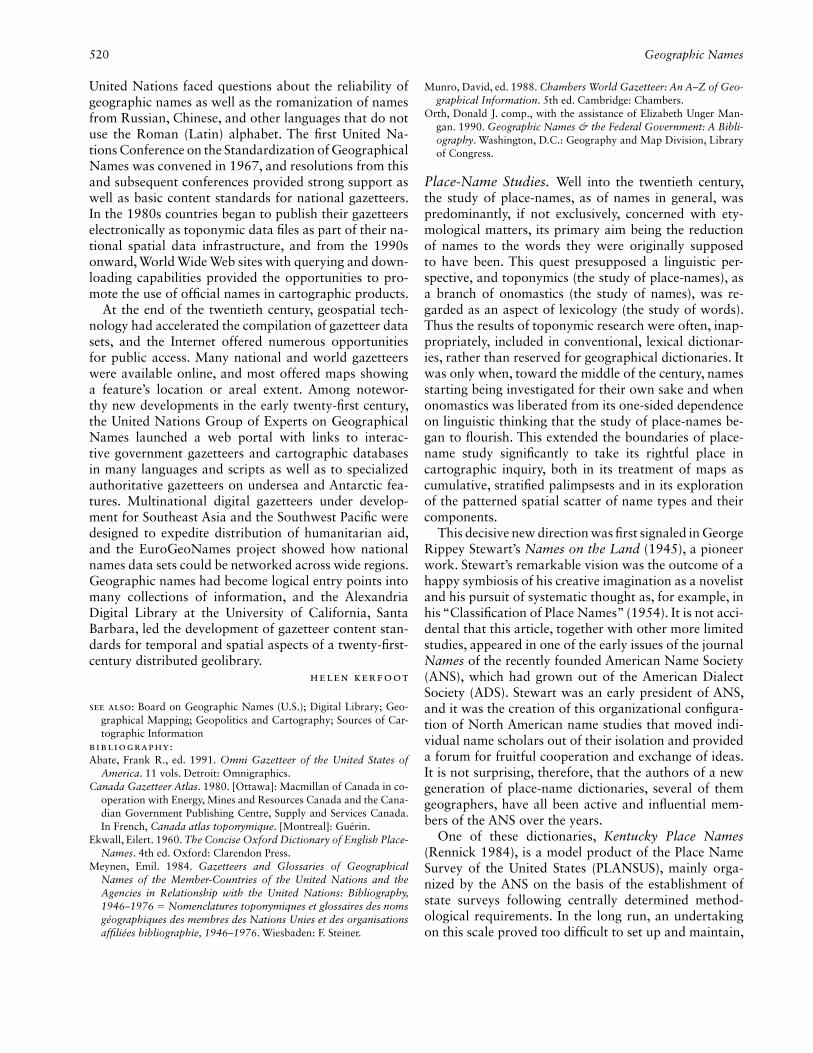
520 Geographic Names

United Nations faced questions about the reliability of geographic names as well as the romanization of names from Russian, Chinese, and other languages that do not use the Roman (Latin) alphabet. The fi rst United Na-tions Conference on the Standardization of Geographical Names was convened in 1967, and resolutions from this and subsequent conferences provided strong support as well as basic content standards for national gazetteers. In the 1980s countries began to publish their gazetteers electronically as toponymic data fi les as part of their na-tional spatial data infrastructure, and from the 1990s onward, World Wide Web sites with querying and down-loading capabilities provided the opportunities to pro-mote the use of offi cial names in cartographic products.

At the end of the twentieth century, geospatial tech-nology had accelerated the compilation of gazetteer data sets, and the Internet offered numerous opportunities for public access. Many national and world gazetteers were available online, and most offered maps showing a feature’s location or areal extent. Among notewor-thy new developments in the early twenty-fi rst century, the United Nations Group of Experts on Geographical Names launched a web portal with links to interac-tive government gazetteers and cartographic databases in many languages and scripts as well as to specialized authoritative gazetteers on undersea and Antarctic fea-tures. Multinational digital gazetteers under develop-ment for Southeast Asia and the Southwest Pacifi c were designed to expedite distribution of humanitarian aid, and the EuroGeoNames project showed how national names data sets could be networked across wide regions. Geographic names had become logical entry points into many collections of information, and the Alexandria Digital Library at the University of California, Santa Barbara, led the development of gazetteer content stan-dards for temporal and spatial aspects of a twenty-fi rst-century distributed geolibrary.

Helen Kerfoot

See also: Board on Geographic Names (U.S.); Digital Library; Geo-graphical Mapping; Geopolitics and Cartography; Sources of Car-tographic Information

Bibliography:Abate, Frank R., ed. 1991. Omni Gazetteer of the United States of

America. 11 vols. Detroit: Omnigraphics.Canada Gazetteer Atlas. 1980. [Ottawa]: Macmillan of Canada in co-

operation with Energy, Mines and Resources Canada and the Cana-dian Government Publishing Centre, Supply and Services Canada. In French, Canada atlas toponymique. [Montreal]: Guérin.

Ekwall, Eilert. 1960. The Concise Oxford Dictionary of English Place-Names. 4th ed. Oxford: Clarendon Press.

Meynen, Emil. 1984. Gazetteers and Glossaries of Geographical Names of the Member-Countries of the United Nations and the Agencies in Relationship with the United Nations: Bibliography, 1946–1976 = Nomenclatures toponymiques et glossaires des noms géographiques des membres des Nations Unies et des organisations affi liées bibliographie, 1946–1976. Wiesbaden: F. Steiner.

Munro, David, ed. 1988. Chambers World Gazetteer: An A–Z of Geo-graphical Information. 5th ed. Cambridge: Chambers.

Orth, Donald J. comp., with the assistance of Elizabeth Unger Man-gan. 1990. Geographic Names & the Federal Government: A Bibli-ography. Washington, D.C.: Geography and Map Division, Library of Congress.

Place-Name Studies. Well into the twentieth century, the study of place-names, as of names in general, was predominantly, if not exclusively, concerned with ety-mological matters, its primary aim being the reduction of names to the words they were originally supposed to have been. This quest presupposed a linguistic per-spective, and toponymics (the study of place-names), as a branch of onomastics (the study of names), was re-garded as an aspect of lexicology (the study of words). Thus the results of toponymic research were often, inap-propriately, included in conventional, lexical dictionar-ies, rather than reserved for geographical dictionaries. It was only when, toward the middle of the century, names starting being investigated for their own sake and when onomastics was liberated from its one-sided dependence on linguistic thinking that the study of place-names be-gan to fl ourish. This extended the boundaries of place-name study signifi cantly to take its rightful place in cartographic inquiry, both in its treatment of maps as cumulative, stratifi ed palimpsests and in its exploration of the patterned spatial scatter of name types and their components.

This decisive new direction was fi rst signaled in George Rippey Stewart’s Names on the Land (1945), a pioneer work. Stewart’s remarkable vision was the outcome of a happy symbiosis of his creative imagination as a novelist and his pursuit of systematic thought as, for example, in his “Classifi cation of Place Names” (1954). It is not acci-dental that this article, together with other more limited studies, appeared in one of the early issues of the journal Names of the recently founded American Name Society (ANS), which had grown out of the American Dialect Society (ADS). Stewart was an early president of ANS, and it was the creation of this organizational confi gura-tion of North American name studies that moved indi-vidual name scholars out of their isolation and provided a forum for fruitful cooperation and exchange of ideas. It is not surprising, therefore, that the authors of a new generation of place-name dictionaries, several of them geographers, have all been active and infl uential mem-bers of the ANS over the years.

One of these dictionaries, Kentucky Place Names (Rennick 1984), is a model product of the Place Name Survey of the United States (PLANSUS), mainly orga-nized by the ANS on the basis of the establishment of state surveys following centrally determined method-ological requirements. In the long run, an undertaking on this scale proved too diffi cult to set up and maintain,

Geographical Mapping 521

and the question remains whether a political administra-tive unit, like a state, is the most appropriate or manage-able organizational principle, since so much toponymic evidence crosses state boundaries, as demonstrated by the atlas This Remarkable Continent (Rooney, Zelinsky, and Louder 1982). The result of another ambitious co-operative venture, the North American Cultural Survey, Remarkable Continent contains more than 300 pages and more than 1,300 maps, already in existence at the time of its compilation, including place-name distribu-tion maps. As is to be expected, the editors and other scholars involved in this project were mostly cultural geographers, confi rming the conviction that place-name studies benefi ted greatly from the realization that names are much more than just words with peculiar, additional qualities.

This liberation of place-name studies from purely lin-guistic, especially etymological, concerns has resulted in the laying bare of a variety of intra-onymic processes: (a) place-names > surnames: Buckley, Gratton, Lee ming; (b) surnames > place-names: Endicott, Hudson, Jeffer-son; (c) place-names > surnames > place-names: Dal-las, Houston, Washington; (d) transfers of whole place-names from a homeland: Hamburg, Plymouth, Warsaw; (e) cultural transfers of whole place-names: Homer, Ithaca, Syracuse, Vestal. In all these transformations the names in question were completely unanalyzed seman-tically and morphologically. A fascinating illustration is names given to units of the Military Tract in upstate New York, as demonstrated in Wilbur Zelinsky’s study of classical town names that highlighted sociocultural origins and dissemination, derived from “the notion . . . that the United States is the latter-day embodiment of the virtues and ideals of ancient Greece and Rome” (Zelinsky 1967, 463), at a time when the newly inde-pendent country was looking for its post colonial iden-tity. A related outcome is the realization that the extent of toponymic dialect areas is not necessarily congruent with that of the linguistic dialect areas of their gener-ics. For instance, the term bayou, “a sluggish stream” in Louisiana, is more extensive in its lexical usage than as a hydronymic generic (Bayou Beaucoup, Bayou Gauche, Bayou Jaune). Thus it becomes clear that the potential of place-names as factors in region-making cannot be overrated.

W. F. H. Nicolaisen

See also: Historians and Cartography; Indigenous Peoples and West-ern Cartography

Bibliography:Rennick, Robert M. 1984. Kentucky Place Names. Lexington: Univer-

sity Press of Kentucky.Rooney, John F., Wilbur Zelinsky, and Dean R. Louder, eds. 1982. This

Remarkable Continent: An Atlas of United States and Canadian So-ciety and Cultures. College Station: For the Society for the North American Cultural Survey by Texas A&M University Press.

Stewart, George Rippey. 1945. Names on the Land: A Historical Ac-count of Place-Naming in the United States. New York: Random House.

———. 1954. “A Classifi cation of Place Names.” Names 2:1–13.Zelinsky, Wilbur. 1967. “Classical Town Names in the United States:

The Historical Geography of an American Idea.” Geographical Re-view 57:463–95.

Geographical Institute De Agostini (Italy). See Isti-tuto Geografi co De Agostini

Geographical Mapping. Defi ned simply as a small-scale map of the entire world or a large region, the geographical map has been ubiquitous throughout the twentieth century, when it interconnected with other modes of mapping practice, most notably administrative mapping, thematic mapping, marine charting, overhead imaging, and dynamic cartography. Though far less dis-tinctive than during the European Enlightenment (Ed-ney 1993), geographical maps have provided scientifi c and scholarly institutions with a generally reliable and often innovative framework for visualizing broad geo-graphic patterns or situations previously represented in a less complete or exact fashion, if at all. The continued vigor of geographical mapping since 1900 refl ects a vo-racious geographical curiosity fueled by expanding tech-nologies for scientifi c measurement as well as a thirst for order and predictability, particularly in disciplines like meteorology and seismology, concerned with forecast-ing disaster, but also in more rhetorical or regulatory endeavors like geopolitics, aeronautical charting, and the Law of the Sea. In highlighting arenas of map use that have relied heavily on geographical maps, this entry pays particular attention to applications that emerged or experienced marked expansion during the twentieth century.

An intriguing new arena for geographical mapping was the aeronautical chart, which emerged in the 1920s as a form of topographic map annotated or specially formatted to serve the way-fi nding needs of aviators. As commercial and military aviation became faster and more common in the 1940s and 1950s, aeronautical charts necessarily covered longer distances at smaller scales and challenged their compilers to integrate a suit-able mix of terrain, political, and navigational features (Ehrenberg 2006). In promulgating diverse restrictions on fl ying, the aeronautical chart produces, reproduces, and regulates navigable airspace and underscores the in-creased use of maps as tools of government. In addition, the growth of continental and intercontinental air car-riers led to small-scale air-route and advertising maps, which helped the traveling public plan an itinerary and select an appropriate carrier.

While the aeronautical chart arose in response to a

522 Geographical Mapping

new, markedly faster mode of transport, journalistic car-tography grew well beyond its nineteenth-century roots with the development of more effi cient technology for copying images and integrating them into the page lay-out of a newspaper or magazine. Although many jour-nalistic maps were more topographic than geographi-cal in both scale and content, global confl ict and other newsworthy events that were continental or global in scope fostered an increased use of geographical maps in the print and electronic media (Monmonier 1989). Geo-graphical maps with a broad geographic scope, and thus informative to readers across a continent or around the world, dominated the cartographic content of illustrated news stories distributed by feature syndicates and wire services, necessarily focused on broad rather than local markets. Even when a news story highlighted a local di-saster or curiosity, a geographical map was often used to locate the site within a broader spatial context.

War and threats of war inspired many geographi-cal maps during World War II and the Cold War that followed, and thus heightened the salience of the long-term relationship between cartography and warfare. Rhetorical maps used to legitimize or refute territorial claims or to frame an invasion or attack as an unavoid-able response to an intolerable threat typically required a geographical, rather than topographic, scale as did maps ostensibly intended more for understanding than for persuasion. In many cases, expository maps could be repurposed to support a political agenda. A case in point is the earth-from-space perspective used by jour-nalistic cartographer Richard Edes Harrison to describe the relative proximity of combatants in World War II (Schulten 2001, 214–26) and modifi ed only slightly dur-ing the late 1940s and early 1950s to promote air-age globalism, which underscored the need to prepare for an over-the-pole missile attack on the United States by the Soviet Union (Henrikson 1975).

Harrison’s global perspective attained greater promi-nence in a different context in the 1960s and early 1970s, when human spacefl ight allowed the Apollo astro nauts to photograph the earth from outer space. Denis E. Cosgrove, who examined the cartographic signifi cance of the National Aeronautics and Space Ad-ministration’s (NASA) Apollo program, identifi ed two iconic photos, taken in 1968 and 1972, on missions 8 and 17. On 24 De cem ber 1968, when Apollo 8 was in orbit around the moon, an astronaut took the much-acclaimed “Earthrise” photograph (see fi g. 349), argu-ably a geographical map, which juxtaposed the lunar surface in the foreground with the much smaller, partly illuminated planet in the distance. “Combined with the deathly lunar surface the photograph suggests the com-plete isolation of terrestrial life in a black, sepulchral universe” (Cosgrove 1994, 275). Although astronauts

fi nally set foot on the moon the following July, the most famous earth-from-space photograph was taken on 7 December 1972, on the way to the moon, by the crew of Apollo 17, the sixth and last mission to land on the lunar surface. Titled the “Whole Earth” by some and the “Blue Marble” by others, the full-disk photograph (see fi g. 350) shows the southern jet stream circling a cloud-covered South Pole and the coastlines of Africa, Madagascar, and the Arabian Peninsula as well as por-tions of Europe and South Asia. According to Cosgrove, both of these images are highly inspirational and can be seen to align with two distinct ideologies: the “one-worldism” of a liberal American Christianity committed to open borders and the “whole-earth” stance of envi-ronmental activists.

Rocketry and space photography not only extended the domain of geographical mapping to include maps and atlases of Mercury, Venus, Mars, and various aster-oids but also substantially enhanced lunar cartography, with roots in the sixteenth century (Whitaker 1999). Compiled from imagery obtained with fl y-by space probes and orbiting sensors, these maps inspired sys-tematic efforts to regulate and inventory the assignment of geographic feature names. On another cartographic frontier, the exploratory mapping and systematic nam-ing of submarine features further blurred the distinction between geographical and topographic mapping (Mon-monier 2006, 134–44).

Satellite remote sensing and image processing afforded other earth-from-space views, including the GeoSphere Image constructed by designer Tom Van Sant as a mo-saic from a multitude of individual NOAA environmen-tal satellite images and used widely in the early 1990s, most notably as the title page of the 1990 edition of the National Geographic Atlas of the World. Van Sant framed his map on a rectangular cylindrical projection with north-south scale reduced in the upper latitudes to partly compensate for areal distortion. He examined months of satellite imagery to select only pixels not com-promised by cloud cover and assigned colors chosen, a bit naively, to show how the terrain might look from an altitude of several thousand miles. His exaggerated claims for a “natural representation” on a hypothetical “clear day” was an opportunity for Denis Wood (1992, 48–69) to demonstrate how rhetoric can be deployed to excoriate an ostensibly clever and harmless—though clearly costly—endeavor.

Rhetoric also featured prominently in debates over the Peters projection (see fi g. 679), a geometric framework for whole-world geographical maps that was proffered and contested several times from the late 1970s through the late 1990s (Monmonier 2004, 145–71; Wood 1992, 56–61). Supporters claimed it was the only appropriate antidote to the Mercator projection’s fl agrant infl ation

Geographical Mapping 523

of relative size (and hence the relative importance) of the more developed nations of North America and Western Europe, and the consequent visual diminution of Third World nations, largely within 30 degrees of the equator. Opponents denounced the equally fl agrant distortion of shape by the Peters map—particularly within 30 de-grees of the equator!—and argued that the Mercator map was seldom used to frame whole-world maps. That the debate gained credibility refl ected the importance of whole-world geographical maps in the popular print media, where much of the contestation occurred.

Whole-world maps proved particularly valuable in the earth sciences, where perceptive contemplation of continental margins and atmospheric circulation re-quired small-scale representations. Although the sugges-tive similarity of the eastern edge of South America and the western coastline of Africa had caught the attention of Abraham Ortelius and Antonio Snider-Pellegrini in the sixteenth and nineteenth centuries, respectively, Ger-man meteorologist Alfred Wegener is the acknowledged discoverer of continental drift, which he eloquently de-scribed in Die Entstehung der Kontinente und Ozeane (1915; 2d ed., 1920) with a three-map graphic narrative showing the juxtaposition of continental landmasses roughly 250, 50, and 1 million years ago (Monmonier 1995, 149–69). In the decades that followed, Wegener’s model invited controversy and at times ridicule, but his compelling visual argument was vindicated in the 1950s and 1960s by geophysical and hydrographic explora-tions, which yielded the comparatively detailed thematic maps that helped develop and confi rm the hypotheses of plate tectonics and seafl oor spreading. Textbooks on physical geography eagerly touted an associated phenomenon, the Pacifi c Ring of Fire, with small-scale maps relating the pattern of earthquakes and volcanoes on the rim of the Pacifi c Ocean to continental plate boundaries.

Small-scale maps of weather and climate refl ect a strong interaction among geographical and thematic mapping, overhead imaging, and dynamic cartography (Monmonier 1999). Except for local radar maps and focused studies of microclimates and specifi c storms, atmospheric cartography uses mostly small-scale rep-resentations to track and predict the development and movement of comparatively broad geographical features like pressure cells, air masses, frontal boundaries, and jet streams. Computer models are typically continental or hemispheric in scope, and resolution is low because of the sparse monitoring network and the computational demands of representing vertical differences in pressure, heat energy, and moisture while projecting the map for-ward several days in small increments of time—at cen-tury’s end the smallest cells in dynamic computational models were several kilometers across.

In the fi nal decades of the twentieth century atmo-spheric science turned to global models to predict the extent and impacts of climate change under diverse sce-narios of anthropogenic warming (Monmonier 2008, 131–46). Controversy over the resulting maps refl ected both the inherent uncertainty of computational modeling and the economic consequences of political strategies for reducing concentrations of greenhouse gases known—or merely believed, as so-called skeptics asserted—to cause global warming. Especially problematic were scenarios refl ecting the disappearance of ice shelves in Antarctica and Greenland. Topographic as well as geographical maps described both local and broad impacts, and dy-namic simulations dramatized consequences by com-pressing time. Because the direction of climate change was more certain than its timing, maps describing plau-sible impacts of sea level rise decades or centuries in the future typically focused on elevation, with no specifi c year-date in either title, key, or caption.

With water covering nearly three-quarters of the earth’s surface, geographical maps were especially use-ful in the latter half of the twentieth century, when in-ternational treaties known collectively as the Law of the Sea not only extended territorial waters well away from the shore but allowed maritime nations to claim fi sh-ing and subsurface mining rights within so-called Exclu-sive Economic Zones (EEZs). The typical EEZ extended 200 nau tical miles outward from the shoreline, except where EEZs overlapped or an extension of the continen-tal shelf allowed an even broader zone, up to 350 nauti-cal miles wide (Monmonier 2008, 102–13).

Century’s end left the geographical map with a sig-nifi cant supporting role in cartographic endeavors more numerous and diverse than those examined here. None-theless, the pure geographical map—the small-scale general-purpose reference map—survived in several for-mats, most notably as wall maps, world and regional reference maps at the front or back of world and na-tional atlases, and the smaller-scale views afforded by dynamic web maps and electronic atlases, including vir-tual globes with zoom and pan functionality. The latter provided a fi tting replacement for the International Map of the World, a complicated endeavor undermined by questionable specifi cations, most notably its 1:1,000,000 scale, which Arthur H. Robinson (1965, 24) denounced as “too small for one to plot fi eld observations, but . . . suffi ciently large to make a general purpose map series quite cumbersome.” Zooming and panning freed the geographical map from the tyranny of sheet lines and a rigid level of detail.

Mark Monmonier

See also: Air-Age Globalism; Atlas: World Atlas; Geographic Names: Gazetteer; Projections: (1) World Map Projections, (2) Regional Map Projections; International Map of the World; Wall Map

524 Geography and Cartography

Bibliography:Cosgrove, Denis E. 1994. “Contested Global Visions: One-World,

Whole-Earth, and the Apollo Space Photographs.” Annals of the Association of American Geographers 84:270–94.

Edney, Matthew H. 1993. “Cartography without ‘Progress’: Reinter-preting the Nature and Historical Development of Mapmaking.” Cartographica 30, nos. 2–3:54–68.

Ehrenberg, Ralph E. 2006. “‘Up in the Air in More Ways than One’: The Emergence of Aeronautical Charts in the United States.” In Cartographies of Travel and Navigation, ed. James R. Akerman, 207–59. Chicago: University of Chicago Press.

Henrikson, Alan K. 1975. “The Map as an ‘Idea’: The Role of Carto-graphic Imagery during the Second World War.” American Cartog-rapher 2:19–53.

Monmonier, Mark. 1989. Maps with the News: The Development of American Journalistic Cartography. Chicago: University of Chicago Press.

———. 1995. Drawing the Line: Tales of Maps and Cartocontroversy. New York: Henry Holt.

———. 1999. Air Apparent: How Meteorologists Learned to Map, Predict, and Dramatize Weather. Chicago: University of Chicago Press.

———. 2004. Rhumb Lines and Map Wars: A Social History of the Mercator Projection. Chicago: University of Chicago Press.

———. 2006. From Squaw Tit to Whorehouse Meadow: How Maps Name, Claim, and Infl ame. Chicago: University of Chicago Press.

———. 2008. Coast Lines: How Mapmakers Frame the World and Chart Environmental Change. Chicago: University of Chicago Press.

Robinson, Arthur H. 1965. “The Future of the International Map.” Cartographic Journal 2:23–26.

Schulten, Susan. 2001. The Geographical Imagination in America, 1880–1950. Chicago: University of Chicago Press.

Whitaker, Ewen A. 1999. Mapping and Naming the Moon: A History of Lunar Cartography and Nomenclature. Cambridge: Cambridge University Press.

Wood, Denis, with John Fels. 1992. The Power of Maps. New York: Guilford Press.

Geographical Society of the USSR. See Russkoye geografi cheskoye obshchestvo (Russian Geographical Society)

Geographical Survey Institute (Japan). See Kokudo chiriin

Geography and Cartography. The history of geog-raphy is one of exploration and mapmaking followed by the development of an academic discipline that took shape mostly in the twentieth century. In the late nine-teenth century, the key role that geography and map-ping played in colonial trade and imperialism was the basis for the claim that geographical instruction should be a part of school curricula. Newly established geo-graphical societies in Europe and North America argued successfully for the inclusion of geography in the uni-versal school curricula, particularly in Western Europe. Teaching geography in schools required developing

programs in universities to train teachers as well as ad-vance scholar ship. Geography degree programs and de-partments in major universities were needed to give the discipline academic credibility, and geographic societies lobbied hard for their establishment.

The academic research directions taken in the late nineteenth century were set by the work of a few in-fl uential individuals, especially the German scholars Alexander von Humboldt and Carl Ritter, and French geographer Paul Vidal de la Blache. Humboldt’s work was based on fi eld collection of data, particularly from expeditions in Central and South America, and their synthesis through maps, leading to generalizations re-garding environmental observations and their links with human activities. Ritter studied the connections between phenomena in places, now called regional geography. This study was based on defi ning regions, separate areas with distinct assemblages of phenomena, with regional boundaries often drawn on maps. In France, geography was rooted in history and mapping. Vidal de la Blache, who had trained as a geographer, focused on defi ning on maps and describing regions’ relatively small homo-geneous areas whose distinctive genres de vie (modes of life) resulted from the interactions of people with their environment.

Throughout the twentieth century, the fi elds of geog-raphy and cartography have maintained a close rela-tionship. The linkage was established in North America by the founders of U.S. academic geography, whose ap-proach focused on the map as the tool of the geographer. One of the early leaders in establishing the close link between geography and cartography was J. Paul Goode of the University of Chicago (McMaster and Thrower 1991, 151–52). By 1928 he had established a set of classes at Chicago that focused on what is now called thematic cartography. As early as 1928 Goode had de-veloped a course called Graphics and Cartography for the Geographer that focused on what he called visual education. Seminal cartographers who followed, includ-ing Erwin Raisz, Guy-Harold Smith, Arthur H. Robin-son, George F. Jenks, and Waldo R. Tobler, each felt that a strong geographical education was essential for the successful cartographer.

By 1938, in the fi rst American textbook on cartogra-phy, General Cartography, Raisz stated, “Every depart-ment of geography in our institutions of higher learn-ing should include a distinct course in cartography, and there should be a literature on the subject adequate and appropriate to the needs of both teachers and students” (viii). A major part of this book emphasized the needs of geographic cartography including distribution maps, economics maps, maps of geography, and government maps. Raisz’s claim was that “every map is geographic”

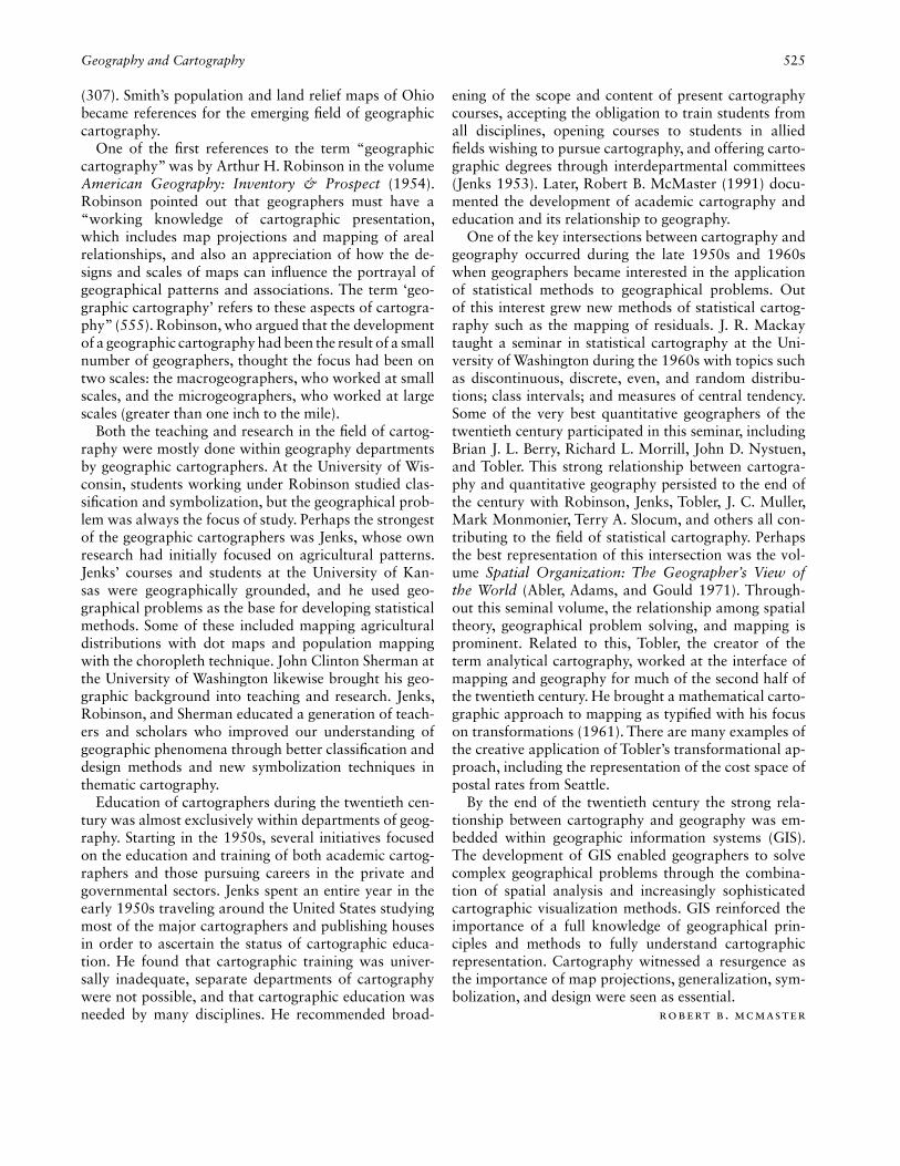
Geography and Cartography 525

(307). Smith’s population and land relief maps of Ohio became references for the emerging fi eld of geographic cartography.

One of the fi rst references to the term “geographic cartography” was by Arthur H. Robinson in the volume American Geography: Inventory & Prospect (1954). Robinson pointed out that geographers must have a “working knowledge of cartographic presentation, which includes map projections and mapping of areal relationships, and also an appreciation of how the de-signs and scales of maps can infl uence the portrayal of geographical patterns and associations. The term ‘geo-graphic cartography’ refers to these aspects of cartogra-phy” (555). Robinson, who argued that the development of a geographic cartography had been the result of a small number of geographers, thought the focus had been on two scales: the macrogeographers, who worked at small scales, and the microgeographers, who worked at large scales (greater than one inch to the mile).

Both the teaching and research in the fi eld of cartog-raphy were mostly done within geography departments by geographic cartographers. At the University of Wis-consin, students working under Robinson studied clas-sifi cation and symbolization, but the geographical prob-lem was always the focus of study. Perhaps the strongest of the geographic cartographers was Jenks, whose own research had initially focused on agricultural patterns. Jenks’ courses and students at the University of Kan-sas were geographically grounded, and he used geo-graphical problems as the base for developing statistical methods. Some of these included mapping agricultural distributions with dot maps and population mapping with the choropleth technique. John Clinton Sherman at the University of Washington likewise brought his geo-graphic background into teaching and research. Jenks, Robinson, and Sherman educated a generation of teach-ers and scholars who improved our understanding of geographic phenomena through better classifi cation and design methods and new symbolization techniques in thematic cartography.

Education of cartographers during the twentieth cen-tury was almost exclusively within departments of geog-raphy. Starting in the 1950s, several initiatives focused on the education and training of both academic cartog-raphers and those pursuing careers in the private and governmental sectors. Jenks spent an entire year in the early 1950s traveling around the United States studying most of the major cartographers and publishing houses in order to ascertain the status of cartographic educa-tion. He found that cartographic training was univer-sally inadequate, separate departments of cartography were not possible, and that cartographic education was needed by many disciplines. He recommended broad-

ening of the scope and content of present cartography courses, accepting the obligation to train students from all disciplines, opening courses to students in allied fi elds wishing to pursue cartography, and offering carto-graphic degrees through interdepartmental committees (Jenks 1953). Later, Robert B. McMaster (1991) docu-mented the development of academic cartography and education and its relationship to geography.

One of the key intersections between cartography and geography occurred during the late 1950s and 1960s when geographers became interested in the application of statistical methods to geographical problems. Out of this interest grew new methods of statistical cartog-raphy such as the mapping of residuals. J. R. Mackay taught a seminar in statistical cartography at the Uni-versity of Washington during the 1960s with topics such as discontinuous, discrete, even, and random distribu-tions; class intervals; and measures of central tendency. Some of the very best quantitative geographers of the twentieth century participated in this seminar, including Brian J. L. Berry, Richard L. Morrill, John D. Nystuen, and Tobler. This strong relationship between cartogra-phy and quantitative geography persisted to the end of the century with Robinson, Jenks, Tobler, J. C. Muller, Mark Monmonier, Terry A. Slocum, and others all con-tributing to the fi eld of statistical cartography. Perhaps the best representation of this intersection was the vol-ume Spatial Organization: The Geographer’s View of the World (Abler, Adams, and Gould 1971). Through-out this seminal volume, the relationship among spatial theory, geographical problem solving, and mapping is prominent. Related to this, Tobler, the creator of the term analytical cartography, worked at the interface of mapping and geography for much of the second half of the twentieth century. He brought a mathematical carto-graphic approach to mapping as typifi ed with his focus on transformations (1961). There are many examples of the creative application of Tobler’s transformational ap-proach, including the representation of the cost space of postal rates from Seattle.

By the end of the twentieth century the strong rela-tionship between cartography and geography was em-bedded within geographic information systems (GIS). The development of GIS enabled geographers to solve complex geographical problems through the combina-tion of spatial analysis and increasingly sophisticated cartographic visualization methods. GIS reinforced the importance of a full knowledge of geographical prin-ciples and methods to fully understand cartographic representation. Cartography witnessed a resurgence as the importance of map projections, generalization, sym-bolization, and design were seen as essential.

Robert B. McMaster

526 Geologic Map

See also: Academic Paradigms in Cartography; Scientifi c Discovery and Cartography; Societies, Geographical

Bibliography:Abler, Ronald F., John S. Adams, and Peter Gould. 1971. Spatial Or-

ganization: The Geographer’s View of the World. Englewood Cliffs: Prentice-Hall.

Jenks, George F. 1953. “An Improved Curriculum for Cartographic Training at the College and University Level.” Annals of the Asso-ciation of American Geographers 43:317–31.

McMaster, Robert B., and Norman J. W. Thrower. 1991. “The Early Years of American Academic Cartography: 1920–45.” Cartography and Geographic Information Systems 18:151–55.

McMaster, Robert B., ed. 1991. “U.S. National Report to ICA, 1991—History and Development of Academic Cartography in the United States.” Cartography and Geographic Information Systems 18:149–216.

Raisz, Erwin. 1938. General Cartography. New York: McGraw-Hill.Robinson, Arthur H. 1954. “Geographical Cartography.” In Ameri-

can Geography: Inventory & Prospect, ed. Preston E. James and Clarence Fielden Jones, 553–77. Syracuse: For the Association of American Geographers by Syracuse University Press.

Tobler, Waldo R. 1961. “Map Transformations of Geographic Space.” PhD diss., University of Washington.

Geoid. See Figure of the Earth

Geologic Map. At the outset of the twentieth century geologic maps were still largely prepared and published using methods that would have been familiar to the eighteenth-century innovators who established geology as a science. Although the digital paradigm shift had completely revolutionized the dissemination of knowl-edge about subsurface phenomena by the year 2000, geologic maps entered the new millennium with a strong imprint of their analog predecessors as well as a digital future impelled by innovative developments in science and technology, particularly in the observation, collec-tion, and application of earth science data and the dis-play of geological knowledge derived therefrom. These enhancements refl ect changes in society as well as sci-entifi c advances. Two world wars saw intense activity in the application of geologic mapping to discover and delineate energy and mineral resources, and population growth and urban and industrial expansion necessitated a focus on water as both a natural hazard and a scarce, fragile resource. Novel investigative techniques, includ-ing remote sensing, provided new perspectives, and the acceptance of plate tectonic theory in the 1960s forced geoscientists to rethink the genesis of rocks and related interpretations. In this milieu of change, geologists and geological cartographers readily adopted and adapted wider developments in cartography and spatial data technology.

A traditional geologic map depicts rock type, classi-fi ed and colored according to the lithology of the rocks, e.g., sandstone, their age (chronostratigraphy), or their lithology and stratigraphic position (lithostratigraphy)

(fi gs. 314 and 315). Throughout the century a deepening understanding of stratigraphy, made possible through developments in biostratigraphy (in essence using fossils for correlation) and physical and chemical techniques for age-dating, signifi cantly improved the calibration of rocks and allowed the fi eld geologist to produce maps of considerably increased resolution and detail. In ad-dition, a steadily growing number of boreholes drilled for water, civil engineering studies, and mineral explora-tions added to an evidence base enriched by improved geophysical techniques. This increased information threatened both the appearance and the effectiveness of the geologic map, often regarded as an object of consid-erable aesthetic beauty but vulnerable to geologist au-thors eager to include almost everything that they knew of their territory. When a single map was used as both a scientifi c notebook and a means of communication, the latter often suffered.

Geologic maps had another, related weakness. Unsur-passed as a means of communication among geologists, they are, however beautiful, largely dense and arcane to those outside the profession. Moreover, a fundamental characteristic of geologic maps refl ects geology’s role as an interpretive discipline—unlike topographic maps, which are rooted in measurement and often touted as objective, geologic maps are based largely on inference. Laypeople rarely recognize geology as a “detective” sci-ence and the geologic map as only an approximation of reality based on the evidence available. During the lat-ter half of the twentieth century, geoscientists sought to avoid miscommunication by converting the traditional geologic map, with its basic depiction of rock type and age, into “applied” or “thematic” variants designed to describe more explicitly such phenomena as the stability of the ground or the location and extent of mineral re-sources. Equally important, the very best of these applied maps also express the geologist’s confi dence in these in-terpretations. Explicit recognition of uncertainty made otherwise mysterious correlations and associations ac-cessible to public offi cials, investors, and other users.

Central to the evolution of geologic maps were the offi cial geological surveys, staffed by professional sci-entists and technicians and funded by national or pro-vincial governments. By 1900, sixty-fi ve years after the creation of the fi rst national geological survey in Great Britain, geological surveys throughout the world were busily engaged in mapping the rocks of their territories. Although other bodies and individuals, particularly in academe and commerce, also produced geologic maps, offi cial survey organizations produced most of the twentieth century’s geologic maps and made key con-tributions to the development of mapping techniques. Expansion of geologic mapping worldwide refl ected dif-ferences in economic and social development, and geo-

Geologic Map 527

logical surveys evolved differently in different countries, typically progressing from exploration of the territory, through searching for mineral and energy resources, to mitigating hazards and protecting the environment. By 2000 the typical geological survey’s mission had grown to include the impacts of climate change on the ground.

In the second half of the century many geological surveys that had expanded their infl uence to their na-tion’s colonies at the turn of the century began, some-what paradoxically, to incorporate techniques applied internationally in their domestic mapping campaigns. Geophysics, geochemistry, applied mineralogy, and pho-togeology (aerial photographic interpretation) became part of the geological survey mainstream, and new vari-ants of geologic map emerged. Around the same time, in the 1950s and 1960s, the stimulus of the search for hy-drocarbon resources led to extensive seafl oor mapping programs, which necessitated new survey techniques and new types of map.

The two world wars shifted the focus of geologic map-ping dramatically, from long-term strategic goals to im-mediate utility, and this restructuring severely affected systematic mapping programs. Routine geologic mapping intended eventually to provide complete, uniform territo-rial coverage was largely abandoned as maps and reports on battle zones, energy, and industrial minerals were produced to aid the war effort. Topographic base maps, essential as a framework for geologic mapping, became impossible to obtain as their surveyors were diverted to military priorities, and a paper shortage only com-pounded the problems. Even so, the disruptions were not wholly unconstructive: the two calamitous wars and their intervening years produced valuable experience as well as a focus on societal relevance, within geological surveys in particular, that would stand them and their users in good stead for the decades that followed. The needs of nations at war brought into sharp focus the dependence of soci-ety on the resources and properties of the rocks beneath their feet. If geologic science and mapping had been born of curiosity about our natural history in the eighteenth century, in the fi rst half of the twentieth century it had, beyond doubt, matured into an applied science.

Throughout the century geology as a science enjoyed progressive development as well as a progressive par-tition into various subdisciplines. Advances were made across subfi elds, most notably in seismology, hydrogeol-ogy, and economic geology, and most advances resulted in new forms of the geologic map. Moreover, the mid-1960s saw the emergence of the single most revolution-ary development in understanding the earth since the theory of uniformitarianism and birth of geology: plate tectonics. Since the fi rst two decades of the century, when fi rst Frank B. Taylor and then Alfred Wegener had sought to explain the confi guration of the continents,

geologists had struggled to establish a coherent model that placed continental drift, seafl oor spreading, and seismic and volcanic activity within a consistent con-text. The theory of plate tectonics provided that unify-ing concept, which affected all areas of the geosciences, including geologic mapping and its products. Although theory normally follows evidence, rocks and maps of rocks had to be reappraised around the world in light of this groundbreaking discovery.

Because changes in basic techniques for producing geologic maps occurred at different times in different parts of the world, the dates that follow are only ap-proximations. In 1900 copperplate engraving was still a common method of production. This was succeeded around 1920 by lines and letters drawn by hand in ink on paper or thin enamel board; reference copies were hand-colored using watercolor paints. In the 1960s geo-logic linework was drawn in ink on plastic fi lm, and typed lettering printed on a wax backing was cut out and stuck down in appropriate positions on a separate overlay. The 1970s witnessed the wide adoption of pho-tomechanical reproduction techniques, whereby geo-logic lines were inscribed on a sheet of thin plastic fi lm called scribecoat by using a graver with a sapphire point to cut out their delineations on the fi lm’s photographi-cally opaque coating; the fi lm thus held a negative image of the map’s linework. In addition, peelcoats were used to produce printing masks by hand. By the 1980s com-puter-controlled plotters were producing scribed images and peelcoats for lithographic printing.

In the 1960s and 1970s early experimentation with geological cartographic computing led to equipment and procedures for capturing and displaying geologic data. Innovations in computer graphics technology and geographic information system (GIS) software spawned operational, off-the-shelf systems for map production in the 1980s. The fact that geologic maps were part of an interpretive scientifi c process, and not merely represen-tations of what could be observed, undoubtedly played a role in an early move away from comparatively primi-tive computer-aided design platforms toward the direct encoding of scientifi c features and objects and a more sophisticated use of digital database technology. By the mid-1990s most geological surveys in the developed world had embraced digital technology for the prepara-tion and printing of their geologic maps, and the leaders in the fi eld had also developed corporate databases in which to store geometry and attributes.

The transition to digital methods in the 1990s was not without challenges. Most mapping geologists were initially reluctant to involve themselves in the migra-tion to a digital world, and into the twenty-fi rst cen-tury it was a struggle to engage them in developing the scientifi c protocols, standards, and discipline essential

Geophysics and Cartography 529

for effi cient computer-based processing. At the same time, cartographers who resented information systems experts and geologists meddling in their domain de-bunked predictions that the map would become merely an ephemeral product of a database. Computer-aided display and analysis were not the only change that ge-ologists and geological cartographers would have to ac-cept: by the end of the century several geological orga-nizations across the globe had begun to explore digital geological fi eld mapping supported by GPS (Global Po-sitioning System) receivers as well as end-to-end digital workfl ows and four-dimensional interactive mapping.

Geology has always been a three-dimensional sci-ence—four-dimensional if one includes time. Through-out much of the twentieth century the interpretation and depiction of the geology of our planet was to a large degree as it had been in the nineteenth century, shackled by the limitations of the two dimensions and infl exibility of paper. Throughout the ages every fi eld ge-ologist has held a mental three-dimensional picture of the piece of the earth’s crust he or she was mapping, a picture substantially poorer when transcribed into a two- dimensional map or cross-section. By the end of the century the digital revolution had begun to release ge-ology and geologists from these fetters. Colorful maps and cross-sections, once understood only by the cogno-scenti, were being replaced by dynamic three- and four-dimensional models and animations. Here, freely avail-able, were new tools and techniques that could not only liberate the doing of the science from its publication and dissemination but also, perhaps more importantly, make clear to decision makers and a wider public the critical relevance of geology to the health and wealth of society. This was an audience that had hitherto perceived geo-logic maps, if it thought of them at all, as attractive but esoteric documents. As the twenty-fi rst century dawned the digital revolution, supercharged by the Internet, had initiated the most radical change to the dissemination and accessibility of geological knowledge since the cre-ation of the geologic map.

Ian Jackson

See also: Cave Map; Cvijic, Jovan; Scientifi c Discovery and Cartog-raphy

Bibliography:Albritton, Claude C., ed. 1963. The Fabric of Geology. Stanford: Free-

man, Cooper.Annual Reports of the Geological Survey of Great Britain/The Insti-

tute of Geological Sciences/British Geological Survey. 1900–1999. Nottingham, U.K.

Bickmore, David P., and B. Kelk. 1972. “Production of a Multi-colour Geological Map by Automated Means.” Proceedings of the Interna-tional Geological Congress, 24th Session, Section 16:121–27.

Bonham-Carter, Graeme. 1994. Geographic Information Systems for Geoscientists: Modelling with GIS. New York: Pergamon.

Ireland, H. A. 1943. “History of the Development of Geologic Maps.” Bulletin of the Geological Society of America 54:1227–80.

Nickless, E. F. P., and Ian Jackson. 1994. “Digital Geological Map Pro-duction in the United Kingdom—More Than Just a Cartographic Exercise.” Episodes 17:51–56.

Price, Raymond A. 1992. “National Geological Surveys: Their Present and Future Roles.” Episodes 15:98–100.

Vine, F. J., and Drummond H. Matthews. 1963. “Magnetic Anomalies over Oceanic Ridges.” Nature 199:947–49.

Wegener, Alfred. 1915. Die Entstehung der Kontinente und Ozeane. Brunswick: Friedr. Vieweg & Sohn.

Geophysics and Cartography. At the start of the twentieth century, geophysics was not a recognized dis-

(Facing page)Fig. 314. WEHRGEOLOGISCHE KARTE DES BOS-NISCH-HERZEGOWINISCH-MONTENEGRINISCHEN GRENZGEBIETES, 1:200,000, 1942. German army geol-ogy map of Bosnia-Herzegovina and Montenegro (Sarajevo sheet), produced by Der Abteilung Technische Wehrgeologie der Waffen SS during World War II, showing drinking water conditions. See fi gure 315.Size of the original: ca. 81.8 × 52.2 cm.

Fig. 315. DETAIL FROM WEHRGEOLOGISCHE KARTE DES BOSNISCH-HERZEGOWINISCH-MONTENEGRINI-SCHEN GRENZGEBIETES. The area shown is about sixty-fi ve kilometers northwest of Sarajevo.Size of detail: ca. 13 × 9.85 cm.

530 Geophysics and Cartography

cipline. The word “geophysics,” originally coined in Ger-man, had developed some currency during the 1890s, particularly in the United States, but more specifi c fi elds such as terrestrial magnetism (geomagnetism), terres-trial gravity, and seismology were more generally recog-nized. Global and regional magnetic maps—essentially updated and extended versions of Edmond Halley’s 1701 map of magnetic variation throughout the Atlantic Ocean—were routinely constructed and widely avail-able in formats based on isogons (lines of constant mag-netic declination) or contoured values of total magnetic intensity. Maps were little used in the other fi elds. For example, although Robert Mallet had produced a global map of earthquake occurrence as early as 1857, apart from a contribution by Fernand de Montessus de Bal-lore (1911), no signifi cant new version of this map was published until the work of Beno Gutenberg and Charles Richter (1949).

Geophysics achieved recognition as a primary scien-tifi c discipline with the establishment of the Interna-tional Union of Geodesy and Geophysics (IUGG) under the auspices of the International Research Council in 1919, drawing together various preexisting indepen-dent international bodies representing subdisciplines as its sections (from 1930 known as associations). At this point, although regional magnetic surveying had con-tinued to develop, especially in the context of marine navigation, other forms of geophysical investigation were constrained by insensitive or cumbersome instru-ments. These instruments typically required observa-tory conditions for successful operation, so consistent measurements of the relevant geophysical parameters were rarely if ever made over a region of the earth. The consequent lack of geographical coverage precluded the production of meaningful maps. Maps were primarily used to identify observing locations.

Early oil explorers recognized the potential for using the torsion balance invented by Baron Loránd Eötvös de Vásárosnamény as a survey tool. The Eötvös torsion bal-ance measures the lateral gradient of the earth’s gravity fi eld, a vector that, in effect, points toward the position of any net excess local subsurface mass. Hydrocarbons tend to gather beneath slowly rising bodies of salt (ha-lite), which are lighter than the sandstone formations within which the salt was initially emplaced. The ductile salt also forms an impervious cap, so salt domes form excellent drilling prospects and, depending on the densi-ties of the salt and sandstone, the torsion balance vector points either toward or away from such structures. In Texas during the 1920s, American geologist Donald C. Barton and colleagues used this instrument to conduct surveys relatively rapidly and to construct local maps of gravity gradient from which exploration prospects could readily be identifi ed (fi g. 316).

Fig. 316. A GRAVITY GRADIENT MAP OVER A SALT DOME, 1929. The Nash Dome, the fi rst hydrocarbon pros-pect located with geophysics in the United States, is identifi ed by the distinctive suite of arrows pointing toward the center of dense caprock above the salt dome.Size of the original: ca. 10.9 × 11.5 cm. From Donald C. Bar-ton, “The Eötvös Torsion Balance Method of Mapping Geo-logic Structure,” in Geophysical Prospecting: Papers and Dis-cussions Presented at Meetings Held at New York, February, 1928, and at Boston, August, 1929 (New York: The Institute, 1929), 416–79, esp. 445 (fi g. 9). Image courtesy of the Texas A&M University Libraries, College Station.

Accurate relative gravity meters, most notably de-signed by physicists Lucien LaCoste and Arnold Rom-berg based on the zero-length spring, were developed during the 1930s. Gravity meters permitted gravity sta-tions to be occupied much more rapidly than with tor-sion balances, at which point the oil exploration indus-try moved toward mapping based on total (scalar) fi eld gravity measurements. Seismic refl ection and refraction profi ling methods were also developed to investigate de-tails of subsurface structure associated with prospects initially identifi ed by surface geological and gravity mapping.

Because gravity changes rapidly with height, raw gravity readings are strongly correlated with topogra-phy, so a series of corrections were routinely applied to adjust readings to what would be observed at a suit-able datum level, usually mean sea level or (later) the World Geodetic System of 1984 (WGS84). These cor-rected readings are known as free-air gravity or, if a further correction for the presence of the topographic mass is applied, Bouguer-corrected gravity. The read-ings, initially charted as posted values, were contoured

Geophysics and Cartography 531

to produce a map suitable for interpretation. High or low values of Bouguer gravity are due to a mass surplus or defi cit beneath, and according to circumstances they might be interpreted either as due to higher or lower densities throughout a region and depth range or to the presence of a specifi c high- or low-density body. The maps indicated the position of such regions. Where the purpose of the study was resource exploration, Bouguer-corrected gravity was frequently supplemented by sub-traction of a known or inferred regional trend so as to emphasize short- wavelength features associated with shallow structures.

During the 1930s and 1940s, the U.S.-based oil explo-ration industry and the U.S. Geological Survey (USGS) Fuels Branch established standard protocols for gravity surveying. Following World War II, other national map-ping agencies began to undertake detailed regional grav-ity surveys, initially onshore and subsequently offshore. This information was presented in the form of maps of free-air or Bouguer gravity.

The relatively large number of aircraft available fol-lowing World War II and advances in electronic instru-mentation and recording devices made airborne surveys of the strength of the earth’s magnetic fi eld not only practicable but essential for navigation over hostile ter-ritories. Mapping methods continued to follow the long-standing techniques of constructing profi les, applying corrections, and transferring measurements to posted-value maps, which were then contoured.

Although gravity and magnetic methods in geophys-ics are frequently lumped together in textbooks, at con-ferences, and even managerially in many organizations, the techniques and methods of analysis differ quite sig-nifi cantly. Small-scale, crustally induced, geographical variation in magnetic fi eld intensity is typically bipolar in character because—whether the result of remnant or induced magnetization—the effect of a magnetized body is to increase the fi eld strength in one direction and to reduce it in the opposite direction. However, the earth’s magnetic fi eld is neither vertically nor horizontally ori-ented except at the magnetic poles and equator, respec-tively, so the resulting anomalies are not symmetric—one limb of a magnetic anomaly is larger, often signifi cantly larger, than the other. Through a relatively complex cal-culation requiring signifi cant computational capability the pattern of anomalies can be transformed to a sym-metric situation, yielding a “reduced-to-pole” (or, less often, “reduced-to-equator”) representation of the fi eld largely free of the effects of the local orientation of the earth’s magnetic fi eld. This process yields signifi cant benefi ts in interpretation, but the high computational cost meant that it was little used until digital computers became widely available.

Maps produced by geophysicists played a key role

in the development of plate tectonics. The similarity of shape between the continental regions on either side of the Atlantic Ocean and the possibility that it represented some sort of separation had been remarked upon since the late sixteenth century. In 1915 meteorologist Alfred Wegener published a lengthy discussion of this idea with some supporting geological and palaeontological evi-dence and some speculation as to how the phenomenon might have been caused.

Geologists Alexander Du Toit and Arthur Holmes supported and developed these ideas. Du Toit discussed the relationships between the continental masses and recognized that a major ocean—which he named the Tethys—had once been present between the northern and southern continents, but was now largely closed. However, these arguments were largely dismissed by the geophysical community. Throughout the various edi-tions of his seminal work, The Earth, and at length in the sixth edition (1976), mathematician Harold Jeffreys argued that the effective viscosity of the interior of the earth determined from tidal observations was too great to permit continental drift, and that if the earth’s crust were somehow decoupled from the mantle, the earth’s rotation would cause the major continental masses to collect at the equator.

At Cambridge University, Jeffreys and geophysicist Edward “Teddy” Crisp Bullard disagreed strongly re-garding the quality of fi t between the South Atlantic continents that had been achieved in a reconstruction by Australian geologist S. Warren Carey. Bullard wondered whether some level on the continental slope might be even more representative of the true margin of the conti-nents than the coastline and asked J. E. Everett, a gradu-ate student with a mathematical background, to quan-tify the degree of fi t at various depths. Everett digitized contours from the relevant Admiralty charts and wrote a computer program to perform the rotations on a sphere and to calculate the best fi t. Geologist A. G. Smith, a research associate, examined the geological evidence in detail and identifi ed potential matches across the north-ern Atlantic. The resulting map of the fi t across the entire Atlantic, taken at the 500-fathom (914 m) contour, was geologically as well as geometrically convincing, in that similar structures could readily be traced from one side to the other, and the few regions of overlap were clearly associated with relatively recent postpartition geological activity (fi g. 317). Presented at an American Geophysi-cal Union (AGU) conference in 1965, alongside palaeo-magnetic evidence that the major continents had moved along different paths and magnetic evidence supporting the viability of seafl oor spreading as a mechanism, this map persuaded many that the earth’s crust was laterally as well as vertically mobile.

The physiographic maps of geologists Bruce C. Heezen

Fig. 317. COMPUTER-GENERATED RECONSTRUCTION OF THE CIRCUM-ATLANTIC CONTINENTS IN 1965.Size of the original: 34.4 × 25.2 cm. From Edward Crisp Bul-lard, J. E. Everett, and A. G. Smith, “The Fit of the Continents

around the Atlantic,” in A Symposium on Continental Drift (London: Royal Society, 1965), 41–51, map between 48 and 49 (fi g. 8). Copyright © 1965, the Royal Society.

Geophysics and Cartography 533

and Marie Tharp at the Lamont-Doherty Geological Observatory (LDGO) in New York were similarly in-fl uential to the development of plate tectonics. They recognized faults offsetting the midocean ridge in the Southern Atlantic and subsequently the Indian Ocean. The vivid illustration of these features by cartographic artist Heinrich C. Berann made the part these structures play in the development of oceanic plates obvious even to nontechnical eyes. Heezen, Tharp, and Berann’s dra-matic images of ocean fl oor topography (see fi gs. 611 and 888), made widely available through the National Geographic Society from 1966, and posted on the walls of geophysicists’ offi ces and student rooms worldwide, became important vehicles for explaining and popular-izing the concepts of plate tectonics, leading to an infl ux of talented recruits to the science in the late 1960s and 1970s.

Seismological mapping provided further important insight into the kinematics of plate movement. At the University of California, Berkeley, during the 1930s, physicist Perry Byerly had devised a method of ana-

lyzing earthquakes by plotting the direction of initial motion (up, down, or unclear) on a projection of the hemisphere beneath the earthquake focus—a map of the earth as viewed at the source of seismic P-waves. As a rule, the fi rst-motion maps of earthquakes can readily be divided into regions of consistently upward (compressional) and downward (dilatational) motion, separated by two lines corresponding to a pair of mu-tually perpendicular planes at the source (fi g. 318). One of these planes corresponds to the causative fault. Other evidence, such as correlation with a major topo-graphic or geological feature or with the geometry of other earthquakes in the region, is required to identify which one. Such correlations are identifi ed by putting small versions of the global fi rst-motion maps onto the regional map.

The establishment of the WWSSN—World-Wide Stan-dardized Seismograph Network (originally WWNSS—World-Wide Network of Standard Seismograph Sta-tions) under the auspices of the United States’ VELA Uniform project from the early 1960s meant that for

Fig. 318. MAP OF EARTHQUAKE FIRST-MOTION SOLU-TIONS THROUGHOUT THE WESTERN AND CENTRAL MEDITERRANEAN. Each of the “beach balls” is itself a map of the earth, divided into regions within which the initial mo-tion of the earthquake is observed as compression (dark) or dilatation (light). The fi gure demonstrates, for example, that the Algerian region is dominated by east-west-oriented com-pressional thrust motion, whereas the very different mecha-

nism in eastern Italy indicates that tension and normal faulting is present.Size of the original: 12.1 × 21.5 cm. From D. P. McKenzie, “Active Tectonics of the Mediterranean Region,” Geophysi-cal Journal of the Royal Astronomical Society 30 (1972): 109–85, esp. 126 (fi g. 9). Copyright © 1972 Blackwell Scien-tifi c Publications. Reproduced with permission of Blackwell Publishing Ltd.

534 Geophysics and Cartography

the fi rst time, reliable, accurately timed readings includ-ing seismogram polarity were available with worldwide coverage. Seismologist L. R. Sykes, also at LDGO, used WWSSN seismograms to locate and map earthquakes very accurately and confi rmed that these were occurring at offsets on the Mid-Atlantic Ridge (fi g. 319). He also demonstrated that the mechanisms of these earthquakes were entirely consistent with the transform-fault model of geophysicist J. Tuzo Wilson, a key consequence of the plate tectonic concept.

Computers were readily adopted by geophysicists as routine tools both for scientifi c analysis and for acquir-ing and processing large quantities of data. At one point it was claimed that more than half of all the computer cycles available worldwide were employed in processing seismic refl ection data for the oil and gas industry. The ever-improving graphical display capabilities of these

systems encouraged geophysical analysts to look for new ways to present and understand the spatial varia-tion of the properties they were measuring, as well as the complex relationships between those properties.

The ability to digitally manipulate spatial data was exploited by the gravity and magnetic communities in several very different ways. Whereas contour maps had previously been constructed by hand as overlays on posted values of original measurements reduced through manual calculations, it became possible to emphasize and analyze features of interest through a wide vari-ety of digital manipulations and to display the results promptly. Long-wavelength variations in the earth’s fi eld could be suppressed so as to emphasize shallow struc-tures associated with oilfi eld prospects, or emphasized to identify features in the deeper crust and upper mantle associated with tectonic activity.

Fig. 319. SEISMICITY OF THE EARTH, 1961–1967. The global map of earthquakes detected in 1961–67, following the development of the World Wide Standard Seismograph Net-work, clearly demonstrated how the earth’s crust is divided into a number of distinct plates. Examination of similar maps prepared for various ranges of earthquake depth showed that, at certain points such as beneath Japan and South America, these plates are bent into the body of the earth and are being drawn into it.

Size of the original: 64.7 × 103.8 cm. From Muawia Bara-zangi and James Dorman, “World Seismicity Maps Compiled from ESSA, Coast and Geodetic Survey, Epicenter Data, 1961–1967,” Bulletin of the Seismological Society of America 59 (1969): 369–80, pl. 1. Permission courtesy of the Seismologi-cal Society of America, Albany, California.

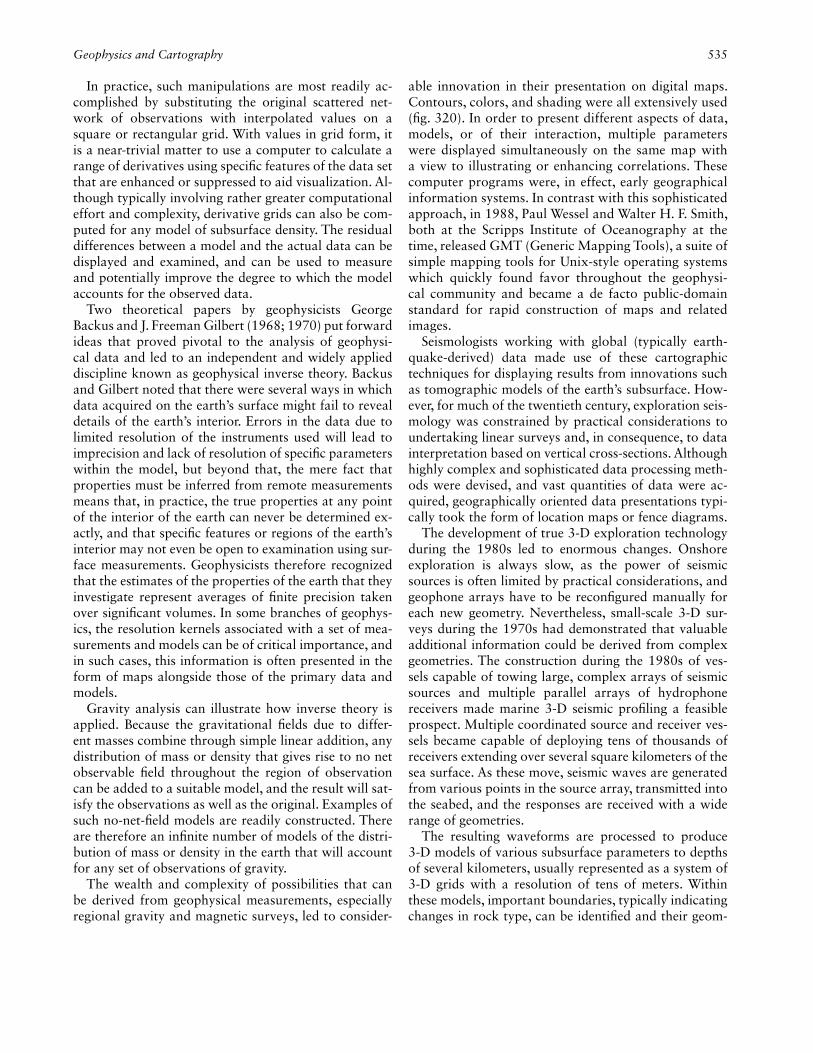
Geophysics and Cartography 535

In practice, such manipulations are most readily ac-complished by substituting the original scattered net-work of observations with interpolated values on a square or rectangular grid. With values in grid form, it is a near-trivial matter to use a computer to calculate a range of derivatives using specifi c features of the data set that are enhanced or suppressed to aid visualization. Al-though typically involving rather greater computational effort and complexity, derivative grids can also be com-puted for any model of subsurface density. The residual differences between a model and the actual data can be displayed and examined, and can be used to measure and potentially improve the degree to which the model accounts for the observed data.

Two theoretical papers by geophysicists George Backus and J. Freeman Gilbert (1968; 1970) put forward ideas that proved pivotal to the analysis of geophysi-cal data and led to an independent and widely applied discipline known as geophysical inverse theory. Backus and Gilbert noted that there were several ways in which data acquired on the earth’s surface might fail to reveal details of the earth’s interior. Errors in the data due to limited resolution of the instruments used will lead to imprecision and lack of resolution of specifi c parameters within the model, but beyond that, the mere fact that properties must be inferred from remote measurements means that, in practice, the true properties at any point of the interior of the earth can never be determined ex-actly, and that specifi c features or regions of the earth’s interior may not even be open to examination using sur-face measurements. Geophysicists therefore recognized that the estimates of the properties of the earth that they investigate represent averages of fi nite precision taken over signifi cant volumes. In some branches of geophys-ics, the resolution kernels associated with a set of mea-surements and models can be of critical importance, and in such cases, this information is often presented in the form of maps alongside those of the primary data and models.

Gravity analysis can illustrate how inverse theory is applied. Because the gravitational fi elds due to differ-ent masses combine through simple linear addition, any distribution of mass or density that gives rise to no net observable fi eld throughout the region of observation can be added to a suitable model, and the result will sat-isfy the observations as well as the original. Examples of such no-net-fi eld models are readily constructed. There are therefore an infi nite number of models of the distri-bution of mass or density in the earth that will account for any set of observations of gravity.

The wealth and complexity of possibilities that can be derived from geophysical measurements, especially regional gravity and magnetic surveys, led to consider-

able innovation in their presentation on digital maps. Contours, colors, and shading were all extensively used (fi g. 320). In order to present different aspects of data, models, or of their interaction, multiple parameters were displayed simultaneously on the same map with a view to illustrating or enhancing correlations. These computer programs were, in effect, early geographical information systems. In contrast with this sophisticated approach, in 1988, Paul Wessel and Walter H. F. Smith, both at the Scripps Institute of Oceanography at the time, released GMT (Generic Mapping Tools), a suite of simple mapping tools for Unix-style operating systems which quickly found favor throughout the geophysi-cal community and became a de facto public-domain standard for rapid construction of maps and related images.

Seismologists working with global (typically earth-quake-derived) data made use of these cartographic techniques for displaying results from innovations such as tomographic models of the earth’s subsurface. How-ever, for much of the twentieth century, exploration seis-mology was constrained by practical considerations to undertaking linear surveys and, in consequence, to data interpretation based on vertical cross-sections. Although highly complex and sophisticated data processing meth-ods were devised, and vast quantities of data were ac-quired, geographically oriented data presentations typi-cally took the form of location maps or fence diagrams.

The development of true 3-D exploration technology during the 1980s led to enormous changes. Onshore exploration is always slow, as the power of seismic sources is often limited by practical considerations, and geophone arrays have to be reconfi gured manually for each new geometry. Nevertheless, small-scale 3-D sur-veys during the 1970s had demonstrated that valuable additional information could be derived from complex geometries. The construction during the 1980s of ves-sels capable of towing large, complex arrays of seismic sources and multiple parallel arrays of hydrophone receivers made marine 3-D seismic profi ling a feasible prospect. Multiple coordinated source and receiver ves-sels became capable of deploying tens of thousands of receivers extending over several square kilometers of the sea surface. As these move, seismic waves are generated from various points in the source array, transmitted into the seabed, and the responses are received with a wide range of geometries.

The resulting waveforms are processed to produce 3-D models of various subsurface parameters to depths of several kilometers, usually represented as a system of 3-D grids with a resolution of tens of meters. Within these models, important boundaries, typically indicating changes in rock type, can be identifi ed and their geom-

536 Geophysics and Cartography

etries as well as their properties imaged. The availability of these models led to much wider use of maps in the seismic exploration industry and to innovation in terms of both the features presented and the display format (fi g. 321). In consequence, the geophysical exploration industry became a major user of geographic information systems (GIS) and a driver of GIS technology from the 1980s onward.

The International Geophysical Year (1957–58 and extended to thirty months), although focused on polar and upper-atmospheric research, attracted much inter-

est in all aspects of the subject, not least because of the important role played by the fi rst artifi cial satellites in that program and the rivalry that developed between the various major nations involved in space science as a result. Later, the GEOS-3 and Seasat satellites that oper-ated between 1975 and 1978, and for just 105 days dur-ing 1978, respectively, both carried laser altimeters to determine the height of the ocean surface. Although the primary purpose of this instrument was oceanographic research—to examine the effect of tides, currents, and storm surges—geodesists including Richard H. Rapp of

Fig. 320. SHADED RELIEF BOUGUER GRAVITY MAP OF THE UNITED KINGDOM REGION. The shading permits short-wavelength structural features such as faults to be read-ily identifi ed, while the color system indicates their relation-ship to the overall pattern of variation in subsurface density. The United Kingdom is outlined in white.

Size of the original: 25.5 × 17.4 cm. From Ian Jackson, ed., Britain Beneath Our Feet: An Atlas of Digital Information on Britain’s Land Quality, Underground Hazards, Resources, and Geology (Keyworth, Nottinghamshire: British Geological Sur-vey, 2004), 19. CP14/017 British Geological Survey © NERC. All rights reserved.

Geophysics and Cartography 537

Ohio State University noted that because the sea sur-face follows the shape of the geoid, variations in geoid topography are due to the distribution of mass or den-sity (Rapp 1979). Sea-surface altimetry can therefore be used to construct maps of the long-wavelength varia-tion in gravity over ocean regions and, after allowing for variation due to ocean depth, of variation in sub-seabed density.

The U.S. National Aeronautics and Space Administra-tion (NASA) launched Geosat in 1986, which operated initially in a Geodetic Mission mode and then in Exact Repeat Mission mode until 1990. Geosat data and re-sults were restricted until the European ERS-1 satellite, carrying a more advanced laser altimeter, was launched in 1995. Declassifi cation of the Geosat data permitted geophysicists David T. Sandwell and Walter H. F. Smith of the Scripps Institute of Oceanography to release their model of gravity throughout the earth’s ocean basins and subsequently a detailed, comprehensive model of the topography of the ocean fl oor reminiscent of the 1960s images of Heezen, Tharp, and Berann. The ERS-1 and TOPEX/Poseidon satellites, operating until 2000 and from 1992 to 2006, respectively, added further in-formation to this data set.

For a six-month period from late 1979, a high-

resolution vector magnetometer satellite, Magsat, oper-ated in a low orbit and produced a global data set suit-able for small-scale mapping applications, within which anomalies due to variations in the earth’s crust are vis-ible. A further high-resolution vector magnetometer sat-ellite, Ørsted, was launched by Denmark in 1999 and operated successfully well into the twenty-fi rst century.

Other satellite systems, not all launched specifi -cally for geophysical purposes, have proved valuable sources of geophysical data. For example, beginning in the mid-1960s, the Defense Meteorological Satel-lite Program (DMSP) operated a series of satellites in sun-synchronous, near-polar orbits. In addition to their primary instruments for observing cloud cover and transmission characteristics, many of these satellites car-ried magnetic and ion sensors. Data from these sensors provide a lengthy history of the earth’s magnetic fi eld and electrical currents at an altitude of about 850 kilo-meters, which have been used in studies of the earth’s ionosphere and its behavior, as well as a variety of solar-terrestrial phenomena.

During the early 1990s, teams at NASA’s Jet Propul-sion Laboratory devised ways to combine synthetic ap-erture radar (SAR) images of a region taken at different times interferometrically, allowing them to detect milli-meter changes in topography. The InSAR technique al-lows deformation of the earth’s surface to be observed and monitored directly over a wide area. Such deforma-tion may be due to earthquakes, subsidence, or human activity such as fl uid extraction. Geophysicist Didier Massonnet and colleagues applied the InSAR technique to the magnitude 7.3 earthquake that occurred near Landers, California, in 1992 (fi g. 322). It was subse-quently recognized that coherent refl ections from rela-tively small individual features including structures such as buildings, preinstalled retro-refl ectors, or even natu-ral features could also be tracked, allowing very detailed studies of local motion to be conducted and motion maps created.

Russ Evans

See also: Astrophysics and Cartography; Figure of the Earth; Inter-national Geographical Union; International Geographical Year; Molodenskiy, M(ikhail) S(ergeyevich); Scientifi c Discovery and Cartography; Tharp, Marie

Bibliography:Backus, George, and J. Freeman Gilbert. 1968. “The Resolving Power

of Gross Earth Data.” Geophysical Journal of the Royal Astronomi-cal Society 16:169–205.

———. 1970. “Uniqueness in the Inversion of Inaccurate Gross Earth Data.” Philosophical Transactions of the Royal Society of London, A. Mathematical and Physical Sciences 266:123–92.

Becker, George F. 1904. “Present Problems of Geophysics.” Science 20:545–56.

Everett, J. E., and A. G. Smith. 2008. “Genesis of a Geophysical Icon: The Bullard, Everett and Smith Reconstruction of the Circum- Atlantic Continents.” Earth Sciences History 27:1–11.

Fig. 321. FRACTURE ORIENTATIONS AND MAGNITUDE OF SEISMIC ANISOTROPY. Careful analysis of 3-D seismic data permits physical properties at depth in the earth to be mapped precisely and in detail. Here, the orientations of frac-tures in a section of the Valhall chalk reservoir are indicated, along with (in color) the magnitude of the seismic anisotropy, from which the fracture information was derived.Size of the original: 7.2 × 8.7 cm. From Stephen A. Hall, J-Michael Kendall, and Olav I. Barkved, “Fractured Reservoir Characterization Using P-Wave AVOA Analysis of 3D OBC Data,” Leading Edge 21 (2002): 777–81, esp. 780 (fi g. 7).

538 Geophysics and Cartography

Fig. 322. INTERFEROMETRIC MAP OF DEFORMATION DUE TO THE LANDERS, CALIFORNIA, EARTHQUAKE, 1992. Interferometric analysis of synthetic aperture radar im-ages before and after the Landers earthquake of 1992 showed the deformation of the earth’s surface that occurred, not only

on the fault itself but throughout the region affected. Data were acquired by European Remote Sensing satellite (ERS-2) on 24 April 1992 and 18 June 1993.Image courtesy of the Jet Propulsion Laboratory, Pasadena.

Good, Gregory, ed. 1994. The Earth, the Heavens and the Carnegie Institution of Washington. Vol. 5 of History of Geophysics. Wash-ington, D.C.: American Geophysical Union.

Gubbins, David, and Emilio Herrero-Bervera, eds. 2007. Encyclopedia of Geomagnetism and Paleomagnetism. Dordrecht: Springer.

Gutenberg, Beno, and Charles Richter. 1949. Seismicity of the Earth and Associated Phenomena. Princeton: Princeton University Press.

Howarth, Richard J. 2007. “Gravity Surveying in Early Geophys-ics: II. From Mountains to Salt Domes.” Earth Sciences History 26:229–61.

Geopolitics and Cartography 539

Jeffreys, Harold. 1976. The Earth: Its Origin, History and Physical Constitution. 6th ed. Cambridge: Cambridge University Press.

Mallet, Robert. 1857. Seismographic Map of the World, Showing the Surface Distribution in Space of Earthquakes. In Mallet’s “Fourth Report upon the Facts and Theory of Earthquake Phenomena,” Re-port . . . of the British Association for the Advancement of Science (1958), published 1859, 1–136, pl. XI.

Massonnet, Didier, and Kurt L. Feigl. 1998. “Radar Interferometry and Its Application to Changes in the Earth’s Surface.” Reviews of Geophysics 36:441–500.

Montessus de Ballore, Fernand de. 1911. La sismologie moderne: Les tremblements de terre. Paris: Armand Colin.

Nettleton, L. L. 1940. Geophysical Prospecting for Oil. New York: McGraw-Hill.

Rapp, Richard H. 1979. “Geos 3 Data Processing for the Recovery of Geoid Undulations and Gravity Anomalies.” Journal of Geophysical Research 84, no. B8:3784–92.

Geopolitics and Cartography. Geopolitics is a form of geographic inquiry that contains a program for politi-cal action. It prioritizes the national interest and is prem-ised on the idea that the geographic environment has a determining infl uence on humans. It analyzes power relations between states by focusing on geographic con-straints and opportunities for human action. The goal is to maximize the power of one’s own state in the quest for global dominance. Although the environmental deter-minist roots of this type of thinking can be traced back as far as Aristotle, it did not emerge as an established school of thought until the beginning of the twentieth century, a few years after Swedish political scientist Ru-dolf Kjellén coined the term geopolitisk in 1899 (Holdar 1992).

Maps are ideally suited for geopolitical inquiry. First, they make it easy to silence alternative explanations or unwelcome details. Geopolitical representations, some-times called territorial codes or geographs, provide frames that offer structured explanations of how to interpret the world. Maps help in the constructions of such frames because their symbols impose hierarchies and order. Second, the causal link between environmen-tal condition and human action that geopolitics strives to prove can be suggested in a convincing manner sim-ply by showing spatial covariation of two phenomena. The anthropometric maps of Ellsworth Huntington are good examples (Livingstone 1994, 141–44). Finally, maps have a cloak of scientifi c respectability and au-thority due to their association with positivist objectiv-ity and precision as well as with state power (Harley 1988). Geopolitical reasoning needs such legitimation to convince those in power to put concepts in action.

Geopolitics emerged during the intensifi ed competi-tion among states at the end of the nineteenth century. Three factors were key: the general realization that the world was fi nite, the declining importance of religious explanations, and rapid technological change. The fa-mous scramble for Africa at the Berlin Conference of

1885 drove home the point that the world was fi nite and that rivalries could no longer be diffused by the discovery of new lands. This new conception of global space set the stage for change, while new nineteenth-century philosophies of evolution and positivism pro-vided the driving ideology and challenged conventional explanations based on an uncritical faith in God. It also added the dire warning of a future struggle grounded in Herbert Spencer’s notion of survival of the fi ttest. Tech-nological change and rapid capitalist industrialization created new means to conquer space, which destabilized the existing balance of power among states. Railroads allowed the faster and more effi cient land transporta-tion of not only goods but also massive armies, and steamships offered similar advances for the projection of power across the oceans.

Maps were inherently useful for the development and propagation of early geopolitical concepts. Halford John Mackinder traced the historical ebb and fl ow of impe-rial expansion on world maps and identifi ed the key place for global dominance: the heartland. The drain-age of rivers to the Arctic underscored the inaccessibility of sea power into this citadel of land power (fi g. 323). A. T. Mahan illustrated the control of the Gulf of Mex-ico and the Caribbean through a triangle that linked the major maritime choke points with the proposed canal across the Central American isthmus (fi g. 324). By con-trast, Friedrich Ratzel’s (1897) concept of the state as an organism, the earliest theoretical conceptualization of the need for state expansion, did not feature such signature maps.

While maps generally accompanied geopolitical texts, especially those directed at a broad audience—for exam-ple, Mahan published in the popular magazines Harper’s and Atlantic Monthly—the full potential of cartographic representations for geopolitical concepts was realized only toward the end of World War I. One factor was that geopolitical reasoning acquired a greater urgency in the turmoil of war and especially in the postwar redrawing of the world political map. The second factor was the perceived effectiveness of British wartime propaganda maps spurred by publications such as Campbell Stuart’s Secrets of Crewe House (1920), which provided detailed explanations of the British propaganda campaign. The two came together for the fi rst time in postwar Germany in a network of geographers and nationalists seeking an effective way to justify a revision of the new boundaries stipulated by the Treaty of Versailles.

Frustrated by the loss of German might, convinced of foreign treachery, and intrigued by British propa-ganda, German geographer Karl Haushofer and sev-eral noteworthy academic collaborators developed a school of thought that came to be known as Geopolitik. They communicated through neoconservative publica-tions and institutions such as Die Grenzboten and the

Fig. 323. HALFORD JOHN MACKINDER’S GEOGRAPHIC PIVOT OF HISTORY.Size of the original: 12 × 18 cm. From Halford John Mac-

kinder, “The Geographical Pivot of History,” Geographical Journal 23 (1904): 421–44, map on 435 (fi g. 5).

Fig. 324. A. T. MAHAN’S STRATEGIC ASSESSMENT OF THE GULF OF MEXICO AND THE CARIBBEAN.Size of the original: 8.9 × 13.2 cm. From A. T. Mahan, Ma-

han on Naval Warfare: Selections from the Writings of Rear Admiral Alfred T. Mahan, ed. Allan F. Westcott (Boston: Little, Brown, 1918), 101.

Geopolitics and Cartography 541

Deutscher Klub in Berlin as well as through secret con-ferences of academics, politicians, and representatives of the government (Herb 1997, 76–84). Starting in 1924, their central forum became the newly founded journal Zeitschrift für Geopolitik.

Followers of this new school of thought believed that Geopolitik should offer (1) a better understanding of the geographical constraints on politics and on state power, (2) a thorough study of Germany’s fair and correct na-tional territory and its rightful place in world politics, and (3) a convincing presentation of these geographi-cal constraints to educate German politicians and the German people about how to bring about change and restore Germany’s status as a world power. Maps were singled out as the most effective means for this purpose, and Haushofer sounded the call for developing a new genre of maps in the early 1920s.

Designed to appeal to the emotions and to exploit psychological principles, these new maps were called “suggestive.” Haushofer explained that Germans had not made such maps before because it was not in their national character. “In contrast to the German carto-graphic representations, the English—because both were a product of the national character, and namely a particularly distinctive one—typifi ed much more and created a more suggestive map image that emphasized the essential and preferably suppressed things that were coincidental or extraordinary; precisely the way En gland molded its people: individually certainly less attractive and complete, often also less insightful and deep, but more useful for a large and collective purpose: man and map!—life-form on earth and its image” (Haus hofer 1922, 17). Even so, Haushofer cautioned that maps could not depict outright lies, which would be easily detected. The key was to omit unwanted detail and to leave out things that did not support the argument. He was convinced that such maps were still truthful and legitimate tools.

Haushofer’s suggestion fell on fertile ground. Over the next few years geopolitical maps were widely dis-seminated through fl yers, textbooks, slide lectures, newspapers, journals, books, and even atlases. Domi-nant themes were the depiction of enemy aspirations (fi g. 325), military vulnerability (fi gs. 326 and 327, and see also fi g. 613), different conceptions of national territory (fi g. 328), and the spread of German culture (fi g. 329). Dissemination of maps was aided by the in-creased use of illustrations in publications in the early twentieth century and especially by liaisons among pub-lishers and pan-German organizations, such as Volk und Reich, Deutscher Schutzbund, and Verein für das Deutschtum im Ausland (Herb 1997, 88–94).

There was remarkable design conformity in sugges-tive maps in their bold black-and-white contrast and heavy use of geometric shapes, such as circles, triangles,

and especially arrows. The latter was the ideal symbol to express the dynamic character of geopolitical con-ceptions. Suggestive maps also had clear links to inno-vations in German graphic design at this time. Arnold Hillen Ziegfeld (1935) advocated the term Kartographik for this new type of map in analogy to the new fi eld of Gebrauchsgraphik (commercial art). Edoardo Bo-ria (2008, 301–2) argues that geopolitical cartography of the period might even have been infl uenced by the Italian futurist movement and Otto Neurath’s work on visualization.

By the early 1930s, suggestive maps were so widely used that Rupert von Schumacher (1934; 1935) felt compelled to develop a theory of design and a gram-mar of geopolitical symbology. He offered a frame-work for designing geopolitical maps for two different audiences—scientifi cally trained readers more tolerant of complexity, and the general public—and presented a catalog of 130 symbols classifi ed under eleven subject headings for topics such as attack, encirclement, and blockade (Schumacher 1935, 256–65). Tellingly, arrows were visually blatant and constituted over one-third of the symbols. The effect of the new design theory is dif-fi cult to gauge. It was developed after several key cartog-

Fig. 325. GERMAN SUGGESTIVE MAP DEPICTING PLANS BY THE CZECH NATIONALIST HANUŠ KUFFNER FOR THE DISMEMBERMENT OF GERMANY. The categories in the legend are, from the top: (1) the Czech bastion (after Kuff-ner: mutilated Czech lands), (2) the Czech glacis lands (after Kuffner: the essential extension of the Czech state), and (3) the Czech approaches in the north and south. The map also ap-peared in other publications.Size of the original: 11 × 11.8 cm. From Rupert von Schu-macher and Hans Hummel, Vom Kriege zwischen den Kriegen: Die Politik des Völkerkampfes (Stuttgart: Union Deutsche Ver-lagsgesellschaft, 1937), 41.

542 Geopolitics and Cartography

raphers, notably Friedrich Lange, Kurt Trampler, Dora Nadge, and especially Ziegfeld, had already developed a unique style and made names for themselves (Herb 1997, 93–94). The theory was as much a survey of past achievements as a new set of rules.

Even though suggestive geopolitical maps were part of a successful strategy to convince the German popu-lation of the rightfulness of territorial expansion, Nazi offi cials were little involved. First, there were conceptual differences between the National Socialist focus on race and the Geopolitik emphasis on space (Bassin 1987). Second, the network of Geopolitik mapmakers contrib-uted to the National Socialist cause on its own, without signifi cant direct involvement in party or offi cial govern-ment endeavors. The Nazis even refrained from employ-ing the most important suggestive cartographer, Zieg-feld, for their wartime map propaganda but recruited him for his experience in having run a publishing fi rm earlier in his career (Herb 1997, 159–60). This lack of collaboration is further apparent in the Nazi atlas The War in Maps (Wirsing 1941), which deviated from the general design practice of geopolitical maps and vio-lated several of the rules of suggestive cartography such as excessive color variation, crude and badly placed let-tering, and the use of what Schumacher (1935, 265) had labeled “nonsensical” symbols (Herb 1989, 300).

The success of geopolitical cartography did not go unnoticed in other states. The 1930s maps of the Ital-ian cartographer Mario Morandi, who worked for the journal Geopolitica, featured strikingly similar designs of arrows and bold black-and-white contrasts (invok-ing good and evil). Yet, Italian geopolitical cartography also had distinct features, such as intricate and complex legends and multiple inserts (fi g. 330) and the produc-tion of atlases for use in schools (Boria 2008). Portugal’s geopolitical maps also were part of the genre (Cairo Ca-rou 2006). By contrast, in the United States geopoliti-cal maps were quickly, albeit falsely, equated with Nazi imperialism and discredited as lies and propaganda (Speier 1941; Strausz-Hupé 1942; Quam 1943). This assessment stuck: in addition to heralding a dismissal of geopolitical concepts as well as a decline in political ge-ography as a whole, it also created the false dichotomy of objective scientifi c maps and propaganda maps, now recognized as fallacious (Crampton and Krygier 2005). The end result was that any map with a captivating mes-sage became suspect.

Geopolitical cartography might have gained greater respect in the United States, where, toward the end of the war, a general recognition of the usefulness of maps for education led to important innovations in geopoliti-cal maps. Walt Disney developed sophisticated animated maps for the fi lm Victory Through Air Power (United Artists, 1943) to effectively present Alexander P. De Seversky’s (1942) new geopolitical concept, air power,

Fig. 326. THREAT TO THE GERMAN EAST AND SOUTH -EAST.Size of the original: 12.9 × 10.5 cm. From Max Hildebert Boehm, Die deutschen Grenzlande, 2d ed. (Berlin: Reimar Hobbing, 1930), 309.

Fig. 327. GERMANY THREATENED BY HEAVILY ARMED NEIGHBORS. The title of the map reads: “Who is disarming?”Size of the original: 7.6 × 10.8 cm. From Albert Ströhle, Von Versailles bis zur Gegenwart: Der Friedensvertrag und seine Auswirkungen (Berlin: Zentralverlag, 1931), 113.

Geopolitics and Cartography 543

with arrows sweeping halfway across the globe to strike the industrial center deep in enemy territory. However intriguing, these animated maps disappeared shortly af-ter the war.

Ironically, De Seversky’s new geopolitical concept also contained the seeds for the demise of geopolitics. In the air age, with long-distance bombers and nuclear mis-siles, not even the forbidding terrain and climate of the Artic could constrain military air strikes. Power projec-tion was no longer determined by the confi guration of the land but simply by the abstract geometric properties of distance and direction. De Seversky’s further develop-ment of his concept in the immediate postwar era clearly reveals this: it identifi ed an abstract geometric area of decision circumscribed by the circular reaches of So-

viet and U.S. airpower across the North Pole (fi g. 331). His map was cast on an azimuthal projection similar to those used by Richard Edes Harrison to vividly describe the global nature of the war against Fascism. But in the 1950s, when De Seversky made his map, the enemy was Communism.

Geopolitics reemerged in the late 1970s, when nuclear parity had made traditional geographic considerations acute for military engagements in different regions and the popularization of geopolitics by Henry Kissinger eclipsed the Nazi stigma (Hepple 1986). Even so, the revitalized geopolitical cartography was comparatively cautious. New conceptions, such as the innovative geo-politics of Yves Lacoste and Hérodote, and Colin S. Gray’s (1977) update of Mackinder’s heartland thesis,

Fig. 328. A NEW CONCEPTION OF NATIONAL TERRI-TORY THAT MAXIMIZES GERMAN CLAIMS THROUGH THE DESIGNATION OF GERMAN CULTURAL SOIL (KULTURBODEN).

Size of the original: 20.6 × 25.8 cm. From Albrecht Penck, “Deutscher Volks- und Kulturboden,” in Bücher des Deu tsch-tums, vol. 1, Volk unter Völkern, ed. Karl C. von Loesch (Bres-lau: Ferdinand Hirt, 1925), 62–73; map between 72–73.

544 Geopolitics and Cartography

which posited that Soviet nuclear submarines could ex-clude American warships from much of the world, were cautious and rather pedestrian in their use of maps (for example, Foucher 1983, 124–25).

A true revival for geopolitical maps came with the publication of a new generation of geopolitical atlases in the 1980s. Spurred by widespread interest in geo-politics across the political spectrum—in addition to the left geopolitics journal Hérodote, which had pro-vided an outlet for Marxist geographers since 1976, a new geopolitics journal on the right, Géopolitique, was published starting in 1983 by the pro-NATO Institut In-ternational de Géopolitique in Paris—atlases during the fi rst decade took on a decidedly realist approach that exposed nuclear threats and east-west and north-south divisions. The most innovative of these early atlases was Gérard Chaliand and Jean-Pierre Rageau’s Atlas straté-gique (1983), which used a variety of projections, ad-dressed different scales, and even included the spatial perceptions of major global players.

After the end of the Cold War, the orientation of geo-political atlases became multipolar as new agendas, such

as the environment, health, and sexual identity, came to the fore. Yet most atlases remained wedded to the basic tenets of a realist tradition; some were even aggressively neoconservative (Vandeburie 2006). In recent years, the focus has been broadened with a forceful presence of the critically left L’atlas: Le monde diplomatique, which has been translated into several languages (Gresh et al. 2006).

This more recent prominence of geopolitical atlases must be placed in historical context. While geopolitical maps have a long history that traces back to the end of the nineteenth century and were widely accepted by the end of the twentieth century, they came into their own as a unique genre only during the heyday of German Geo-politik, between the end of World War I and the end of World War II. Claude Raffestin (2000, 11) even went so far as to argue that “all geopolitical cartography has more or less—and often more rather than less—imitated Ger-man geopolitical cartography.” Deconstructing numer-ous examples of German maps in light of Schumacher’s graphic grammar and Haushofer’s conceptual state-ments, he posited that geopolitical maps are “uchronic” because they seek “to ‘smooth’ and ‘homogenise’ all the deposits of history” and “utopian” because they are “not interested in places in terms of their content but instead, as positions, shapes and surfaces.” Their goal is to depict the geometry of power by the “application of vector calculus” to politics (Raffestin 2000, 24, 26).

However compelling, Raffestin’s argument is limited by its disregard of late-twentieth-century conceptual-izations in critical cartography, such as those of Denis Wood (1992). Raffestin’s reliance on the standard com-munications model permitted him to expose the design tricks of German geopolitical maps as well as the inten-tions behind their creation but prevented him from fully engaging with the larger cultural context of geopolitical cartography. Maps are not mere models of reality that convey unambiguous messages but can be seen as so-cial constructions whose imagery can be interpreted in various and even contradictory ways. Geopolitical maps have to be investigated in the context of human expe-rience and action, not based on their “look or form” (Crampton and Krygier 2005, 17).

Geopolitical maps are embedded in the cultural con-text in which they are created. Mapmakers and their au-diences operate within a commonly shared value system, and the political program the maps contain builds on already existing aspirations for change. In interwar Ger-many, these shared values were the belief in the injus-tice of the Versailles Treaty and the consequent need to revise the borders—values that were shared across the political spectrum. Viewing maps as social constructions reveals that it was not the superior design of suggestive maps that made them effective tools of persuasion, but

Fig. 329. NATURAL BOUNDARIES AND THE LIMITS OF GERMAN CULTURE IN EASTERN EUROPE.Size of the original: 16 × 12.6 cm. From Hermann Lauten-sach, “Geopolitik und staatsbürgerliche Bildung,” Zeitschrift für Geopolitik 1 (1924): 467–76, map on 472.

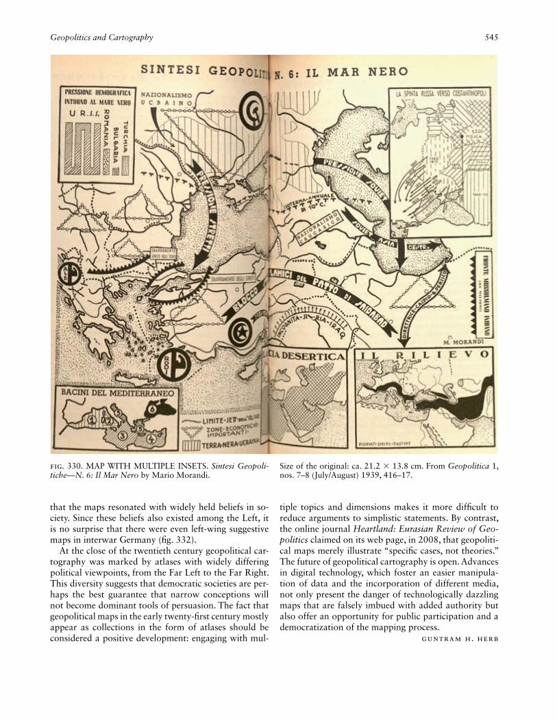
Geopolitics and Cartography 545

that the maps resonated with widely held beliefs in so-ciety. Since these beliefs also existed among the Left, it is no surprise that there were even left-wing suggestive maps in interwar Germany (fi g. 332).

At the close of the twentieth century geopolitical car-tography was marked by atlases with widely differing political viewpoints, from the Far Left to the Far Right. This diversity suggests that democratic societies are per-haps the best guarantee that narrow conceptions will not become dominant tools of persuasion. The fact that geopolitical maps in the early twenty-fi rst century mostly appear as collections in the form of atlases should be considered a positive development: engaging with mul-

tiple topics and dimensions makes it more diffi cult to reduce arguments to simplistic statements. By contrast, the online journal Heartland: Eurasian Review of Geo-politics claimed on its web page, in 2008, that geopoliti-cal maps merely illustrate “specifi c cases, not theories.” The future of geopolitical cartography is open. Advances in digital technology, which foster an easier manipula-tion of data and the incorporation of different media, not only pre sent the danger of technologically dazzling maps that are falsely imbued with added authority but also offer an opportunity for public participation and a democratization of the mapping process.

Guntram H. Herb

Fig. 330. MAP WITH MULTIPLE INSETS. Sintesi Geopoli-tiche—N. 6: Il Mar Nero by Mario Morandi.

Size of the original: ca. 21.2 × 13.8 cm. From Geopolitica 1, nos. 7–8 (July/August) 1939, 416–17.

Fig. 331. ALEXANDER P. DE SEVERSKY’S AIRMAN’S VIEW.Size of the original: 22.4 × 20.3 cm. From Alexander P. De

Seversky, Air Power: Key to Survival (New York: Simon and Schuster, 1950), map between 110–11.

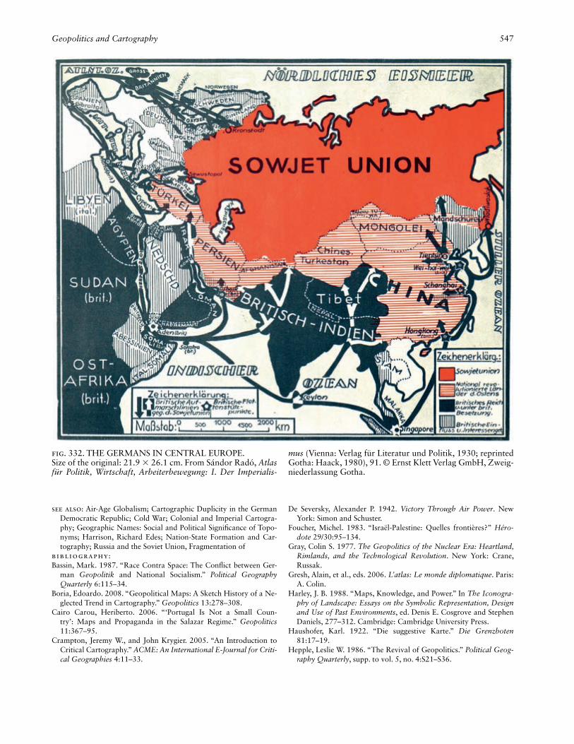
Geopolitics and Cartography 547

See also: Air-Age Globalism; Cartographic Duplicity in the German Democratic Republic; Cold War; Colonial and Imperial Cartogra-phy; Geographic Names: Social and Political Signifi cance of Topo-nyms; Harrison, Richard Edes; Nation-State Formation and Car-tography; Russia and the Soviet Union, Fragmentation of

Bibliography:Bassin, Mark. 1987. “Race Contra Space: The Confl ict between Ger-

man Geopolitik and National Socialism.” Political Geography Quarterly 6:115–34.

Boria, Edoardo. 2008. “Geopolitical Maps: A Sketch History of a Ne-glected Trend in Cartography.” Geopolitics 13:278–308.

Cairo Carou, Heriberto. 2006. “‘Portugal Is Not a Small Coun-try’: Maps and Propaganda in the Salazar Regime.” Geopolitics 11:367–95.

Crampton, Jeremy W., and John Krygier. 2005. “An Introduction to Critical Cartography.” ACME: An International E-Journal for Criti-cal Geographies 4:11–33.

De Seversky, Alexander P. 1942. Victory Through Air Power. New York: Simon and Schuster.

Foucher, Michel. 1983. “Israël-Palestine: Quelles frontières?” Héro-dote 29/30:95–134.

Gray, Colin S. 1977. The Geopolitics of the Nuclear Era: Heartland, Rimlands, and the Technological Revolution. New York: Crane, Russak.

Gresh, Alain, et al., eds. 2006. L’atlas: Le monde diplomatique. Paris: A. Colin.

Harley, J. B. 1988. “Maps, Knowledge, and Power.” In The Iconogra-phy of Landscape: Essays on the Symbolic Representation, Design and Use of Past Environments, ed. Denis E. Cosgrove and Stephen Daniels, 277–312. Cambridge: Cambridge University Press.

Haushofer, Karl. 1922. “Die suggestive Karte.” Die Grenzboten 81:17–19.

Hepple, Leslie W. 1986. “The Revival of Geopolitics.” Political Geog-raphy Quarterly, supp. to vol. 5, no. 4:S21–S36.

Fig. 332. THE GERMANS IN CENTRAL EUROPE.Size of the original: 21.9 × 26.1 cm. From Sándor Radó, Atlas für Politik, Wirtschaft, Arbeiterbewegung: I. Der Imperialis-

mus (Vienna: Verlag für Literatur und Politik, 1930; reprinted Gotha: Haack, 1980), 91. © Ernst Klett Verlag GmbH, Zweig-niederlassung Gotha.

548 GEOSPACE Beckel Satellitenbilddaten GmbH

Herb, Guntram H. 1989. “Persuasive Cartography in Geopolitik and National Socialism.” Political Geography Quarterly 8:289–303.

———. 1997. Under the Map of Germany: Nationalism and Propa-ganda, 1918–1945. New York: Routledge.

Holdar, Sven. 1992. “The Ideal State and the Power of Geography: The Life-Work of Rudolf Kjellén.” Political Geography 11:307–23.

Livingstone, David N. 1994. “Climate’s Moral Economy: Science, Race and Place in Post-Darwinian British and American Geogra-phy.” In Geography and Empire, ed. Anne Godlewska and Neil Smith, 132–54. Oxford: Blackwell.

Quam, Louis Otto. 1943. “The Use of Maps in Propaganda.” Journal of Geography 42:21–32.

Raffestin, Claude. 2000. “From Text to Image.” Geopolitics 5, no. 2:7–34.

Ratzel, Friedrich. 1897. Politische Geographie. Munich: Oldenbourg.Schumacher, Rupert von. 1934. “Zur Theorie der Raumdarstellung.”

Zeitschrift für Geopolitik 11:635–52.———. 1935. “Zur Theorie der geopolitischen Signatur.” Zeitschrift

für Geopolitik 12:247–65.Speier, Hans. 1941. “Magic Geography.” Social Research 8:310–30.Strausz-Hupé, Robert. 1942. Geopolitics: The Struggle for Space and

Power. New York: G. P. Putnam’s Sons.Stuart, Campbell. 1920. Secrets of Crewe House: The Story of a Fa-

mous Campaign. London: Hodder and Stoughton.Vandeburie, Julien. 2006. “Epistemology of Geopolitical Atlases from

the 1980s to the Early 2000s.” Cartographic Journal 43:239–50.Wirsing, Giselher, ed. 1941. The War in Maps, 1939/40. New York:

German Library of Information.Wood, Denis, with John Fels. 1992. The Power of Maps. New York:

Guilford.Ziegfeld, Arnold Hillen. 1935. “Kartengestaltung—ein Sport oder eine

Waffe?” Zeitschrift für Geopolitik 12:243–47.

GEOSPACE Beckel Satellitenbilddaten GmbH (Austria). GEOSPACE Beckel Satellitenbilddaten GmbH is a private Austrian research, publishing, and service company. It was founded in 1984 in Bad Ischl, Austria, by Lothar Beckel, an Austrian geographer who had used aerial photographs since 1967 for his geographi-cal research. Beginning in 1972, when the fi rst Earth Resources Technology Satellite, ERTS 1 (later renamed Landsat 1) was launched by NASA (National Aeronau-tics and Space Administration), Beckel was also involved scientifi cally in the evaluation and application of EOSAT (Earth Observation Satellite Company) image data. In 1994 GEOSPACE relocated to Salzburg.

Established during the beginning phase of commercial-ization of satellite data, GEOSPACE became the Austrian distributor for Spot Image (France) and EOSAT (United States). Its role was to develop the Austrian remote sens-ing market, to provide information and data to poten-tial national users, and to evaluate data for government administration, industry, and education. GEOSPACE became involved in applied research using remote sens-ing data from satellite images and GIS (geographic in-formation systems). GEOSPACE also became one of the national players in earth observation, participating in

many national research projects frequently carried out in cooperation with national research institutions. It also took part in various Framework Programme projects of the European Union, cooperating with international or-ganizations and universities. It worked closely with the ESA (European Space Agency) and with NASA. Those connections continued into the twenty-fi rst century.

In the decade after 2000, GEOSPACE was working on data acquisition by satellite imagery for the support of relief activity during fl oods and for studying dynamic phenomena like precipitation in the tropics and its rela-tionship with vegetative land cover. GEOSPACE under-took conversion of data from land observation satellite systems—SPOT (Satellite Pour l’Observation de la Terre), Landsat, IRS (Indian Remote Sensing Satellite), ERS-1/ERS-2 (European Remote Sensing satellite), Radarsat, NOAA (National Oceanic and Atmospheric Adminis-tration), Meteosat—to images and cartographic prod-ucts in near-natural color. Satellite data were classifi ed for applications in a number of fi elds, including plant sciences, hydrospheric and earth sciences, land use, and land cover. Particular areas of activity were satellite im-age mapping, environment, alpine security, forestry and agriculture, health, cultural heritage, and education.

GEOSPACE made its products available in both printed and digital formats. Its publishing line grew to include satellite image maps (e.g., of Lower Austria, Styria, the Alps, Switzerland), satellite image books and atlases of various countries, and digital atlases on CD-ROM and DVD. Examples include Die Erde neu ent-deckt: Farbige Satelliten-Fotos (1975), Österreich im Satellitenbild (1976), Österreich-Satelliten-Bild-Atlas (1988, updated ed. 2004), Österreich: Ein Porträt in Luft- und Satellitenbildern (1996), and the European Space Agency School Atlas (2007). Satellite image at-lases on CD-ROM offered the possibility of generating three-dimensional views of landscape in true time and of navigating through different landscapes. A special GEOSPACE product was a satellite aeronautical chart of Germany (six sheets, 1:500,000); additional products included city guidebooks of Vienna, Linz, Graz, and Salzburg. Altogether more than 150 publications and studies offer proof of the continuing accomplishments of GEOSPACE.

Ingrid Kretschmer

See also: Remote Sensing: Remote Sensing as a Cartographic Enter-prise

Bibliography:Kretschmer, Ingrid. 2004. “Von der Zweiten Landesaufnahme (1806)

bis zur Gegenwart (2004).” In Österreichische Kartographie: Von den Anfängen im 15. Jahrhundert bis zum 21. Jahrhundert, by In-grid Kretschmer, Johannes Dörfl inger, and Franz Wawrik, ed. Ingrid Kretschmer and Karel Kriz, 168–289, esp. 186–87. Vienna: Institut für Geographie und Regionalforschung der Universität Wien.

Glavnoye upravleniye geodezii i kartografi i 549

Gerrymandering. See Electoral Map

Glavnoye upravleniye geodezii i kartografi i (Chief Administration of Geodesy and Cartography; Russia). Throughout the history of the development of geodesy and cartography in Russia, all work to pro-vide primary geodetic and cartographic base informa-tion was managed by state agencies. Although the state geodetic service was not established until 15 March 1919 by decree of the Sovet narodnykh kommissarov, or Council of People’s Commissars, preliminary discus-sions had begun in Russian intellectual circles and espe-cially in the Imperatorskoye Russkoye geografi cheskoye obshchestvo in the 1880s. In 1916, at the general meet-ing of the Imperatorskoye Rossiyskaya Akademiya nauk, academician Vladimir I. Vernadskiy summed up previous discussions and laid the scientifi c foundations and main guidelines for the state geodetic service (Post-nikov 1988).

From the beginning, the activities of the Vyssheye geodezicheskoye upravleniye (VGU; see table 18 for the organization’s name changes) were connected with those of the Voyenno-topografi cheskaya sluzhba (the military topographic service). The geodetic and carto-graphic activities of both agencies were coordinated by the permanent council board of the military topo-graphical branch of the Red Army’s general headquar-ters, which was established by a 30 May 1925 decree of the Soviet Council of People’s Commissars and the Voyenno- revolyutsionnyi sovet. On 21 April 1940 spe-cial guidelines were approved to coordinate topographi-

cal, geodetic, and cartographic activities conducted by the Glavnoye upravleniye geodezii i kartografi i (GUGK) and the ministry of defense and navy. Those guidelines empowered the GUGK to map all the territories of the Soviet Union except for areas within ten kilometers of naval bases, military installations of the coast guard, state borders, and “the Special Regions” under the juris-diction of the ministry of defense. The latter had to be surveyed by military topographers and navy hydrogra-phers. First-order triangulation, fi rst- and second- order leveling, and fi rst-order astronomical observations be-came the responsibility of the civil geodetic service, with the ministry of defense controlling all the GUGK’s ac-tivities that had military importance. All military and civil surveys and mapping had to conform to the gen-eral rules and programs developed by the GUGK and be coordinated with the ministry of defense. Subsequently, instructions and accuracy standards were developed to provide uniform topographic materials and maps. In 1951 a special meeting of high offi cials from the civil and military topographical agencies fi nally codifi ed these standards and instructions.

The VGU did not start active work until as late as 1922 or 1923. The agency’s evolution refl ected the power struggles between the different Bolshevik fac-tions and leaders of the period. In 1922 there was even an attempt to disband the young agency altogether (Komedchikov 2000, 5–8). The attempt failed and the special scientifi c-technical council of the VGU under Feodosiy Nikolayevich Krasovskiy generated new theo-retical and methodological foundations for topography and geodesy in the country. At fi rst, due to the Civil War

Table 18. As the names of the Glavnoye upravleniye geodezii i kartografi i (GUGK) changed during the twentieth century, so did its form and functions

1919–23 Vyssheye geodezicheskoye upravleniye (VGU) (Higher Geodetic Administration)

1926–28 Geodezicheskiy komitet (Geodetic Committee)

1928–30 Glavnyi geodezicheskii komitet (Chief Geodetic Committee)

1930–32 Glavnoye geodezicheskoye upravleniye (Chief Geodetic Administration)

1933–35 Glavnoye geologo-gidro-geodezicheskoye upravleniye (Chief Geological-Hydrological-Geodetic Administration)

1935–38 Glavnoye upravleniye gosudarstvennoy s”ëmki i kartografi i (GUGSK) (Chief Administration of State Survey and Cartography)

1938–91 Glavnoye upravleniye geodezii i kartografi i (GUGK) (Chief Administration of Geodesy and Cartography)

1991–92 Komitet geodezii i kartografi i (Glavkartografi ya) (Committee for Geodesy and Cartography)

1992–2004 Federal’naya sluzhba geodezii i kartografi i Rossii (Roskartografi ya) (Federal Service for Geodesy and Cartography of Russia)

29 July 2004– Roskartografi ya (Department of Geodesy and Cartography of the Russian Ministry of Transport and Construction)

550 Glavnoye upravleniye geodezii i kartografi i

and other needs of the Bolsheviks, the VGU was unable to organize any new surveys of Russian territory and compile the necessary topographical maps. As a result, Soviet cartographers had to depend on prerevolution-ary cartographic materials. They continued to reprint the most important military topographical maps (with scales of 1, 2, 5, and 10 versts [1 verst = 1.07 kilome-ters] to one inch) and military communication maps us-ing old printing plates.

After the offi cial change to the metric system, the VGU began to compile new topographical maps in the metric system, using old sources but changing the map sym-bols. In the nineteenth century, printed maps with scales larger than 1:420,000 covered only a minor part of the European Russian territory. To make matters worse, the results of some of the surveys of the time were not published. The administrators at the Soviet cartographic service decided to fi nish those works and publish them using new symbols and the metric system. The so-called General Mende’s surveys were the most imposing un-fi nished Russian cartographic project of the nineteenth century. The surveys, which began in 1848 under the supervision of Lieutenant General Aleksandr I. Mende, represented the fi rst coordinated efforts by the country’s main topographical and geodetic services to create a uni-versal topographical map meeting the needs of a broad range of users. The majority of the maps and detailed geographical descriptions drawn up as part of that pro-gram remain at the Russian state archives, Rossiyskiye gosudarstvennyye arkhivy, in manuscript form (Post-nikov 1989, 150–55). By 1926 Soviet cartographers had published some 790 sheets of topographical maps at the scale of 1:100,000 using Mende’s manuscript materials and a few new surveys. In 1929–30, in order to facili-tate the introduction of new technology in geodesy, air survey, and cartography, the Soviet state geodetic survey initiated active contacts with the U.S. Coast and Geo-detic Survey and with such private American fi rms as Brock & Weymouth in Philadelphia.

By the late 1930s, it became obvious that the topo-graphic surveying and mapping of the country was far from fulfi lling the demands of the developing economy. Two categories of large-scale mapping were envisaged under a 1938 plan. The fi rst category included not only European Russia, but also the parts of the Soviet Union under the exclusive control of the Gulag (the main ad-ministration of prisoners’ camps). Depending on the sig-nifi cance of a given region, the mapping was to be per-formed at the scale of 1:10,000, 1:50,000, 1:100,000, 1:200,000, or 1:500,000. By 1941 only a few regions had been surveyed in accordance with the project. Never-theless, Soviet cartographers achieved some real suc-cesses. Detailed and up-to-date atlases such as the fi ve-volume atlas of industry, Atlas promyshlennosti SSSR

(1928–31), the Atlas Moskovskoy oblasti (1933), the Atlas Leningradskoy oblasti i Karel’skoy ASSR (1934), and the two volumes of the Bol’shoy sovetskiy atlas mira (BSAM) (1937–40) were produced and their value ac-knowledged at the Exposition Internationale des Arts et Techniques dans la Vie Moderne in Paris in 1937, where the BSAM was awarded the Grand Prix.

World War II had taught the Soviet leadership a lesson concerning basic large-scale cartography. Learning from that lesson, Joseph Stalin decreed that the fi rst priority for the military and civil state topographical services af-ter the war was a survey of the entire territory of the Soviet Union in preparation for a 1:100,000-scale topo-graphic map. That project, completed in 1954, was gran-diose. The map was based on air surveys performed in the remote regions of Siberia and the Russian Far East, using relatively sparse points of astronomic geodetic control. The network of those control points was ad-justed by phototriangulation. The national topographic map project had nothing to do with providing ordinary consumers with quality large-scale maps. A map at the scale of 1:100,000 fell into the category of secret ma-terials and could not be used even as a source for any general-purpose map.

Large-scale maps for ordinary consumers had to be compiled using the 1:2,500,000-scale map of the Soviet Union, with relevant parts enlarged to the needed scale. In that way tourist maps and maps of administrative units (such as regional and oblast maps), usually com-piled at the sale of 1:600,000, showed only the most general data for main towns, villages, and roads. Even special road maps and atlases for tourists contained no information as to whether the roads were paved with macadam or were stone or dirt.

Limitations on Soviet cartography were relaxed only after perestroika. In 1989 the Voyenno-topografi ches-kaya sluzhba of the General Staff and the GUGK began to publish dependable maps for sale to ordinary con-sumers and for use in business, industry, and agriculture. The maps were at the scale of 1:200,000 and smaller. They were based on topographic maps stripped of mili-tary and other information deemed confi dential (Lyutyy and Komedchikov 1999, 21).

During its nearly ninety years of activity the GUGK has provided the country with a high-precision geodetic control network in a uniform coordinate system. The net includes some 370,000 control points evenly distrib-uted over the country’s territory. A high-precision level-ing network was developed for continental Russia, pro-viding it with heights in the Baltic System. The fi rst-class gravimetric network with a density of one measurement per 100,000 square kilometers was created. In the early twenty-fi rst century it was being developed and updated for the whole country. By then Russia had been fully cov-

Global Positioning System 551

ered with topographic maps at scales from 1:25,000 to 1:1,000,000, while 1:10,000-scale maps were available for 25 percent of Russian territory. The GUGK mapped all towns, settlements, and industrial areas at scales of 1:5,000 to 1:2,000 and sometimes larger.

By the end of the century the right of the state to man-age geodesy and cartography and to name geographi-cal features had been fi xed in the constitution of the Russian Federation. The legal foundations of geodetic and mapping activities were set forth in the Federal Act on geodesy and cartography. The responsibilities of Roskartografi ya were as follows: coordination of geodetic and cartographic activities of the subjects of the Russian Federation with a view to pursue a single technical policy and avoid duplication in geodetic and mapping works fi nanced by the federal budget, the budgets of the subjects of the Russian Federation, and local budgets. It was also responsible for the organiza-tion and execution of geodetic and cartographic works of federal and departmental signifi cance, geodetic and cartographic works ordered by the state authorities of the Russian Federation, self-management bodies, and private individuals.

Roskartografi ya had grown by the early twenty-fi rst century to include twenty aerial-survey geodetic estab-lishments (AGE), three topographic mine-surveying establishments, six geoinformational centers (two of which were a part of aerial geodetic establishments), three mapmaking facilities, the cartographic production association Kartografi ya, two optico-mechanical plants (one of which was a part of an AGE), the Tsentral’nyy nauchno-issledovatel’skiy institut geodezii, aeros”yëmki i kartografi i (TsNIIGAiK), the Gostsentr Priroda, nine-teen territorial departments (which are responsible for inspections) for state geodetic supervision, the Tsen-tral’nyi kartografo-geodezicheskiy fond, the Gosudarst-vennyi kartografi cheskii i geodezicheskii tsentr, and four secondary specialized educational establishments (col-leges). Departments of Roskartografi ya were located in various cities and regions of the Russian Federation, and their production capacities were distributed territorially, each aerial geodetic establishment servicing a certain lo-cality in the Russian Federation within which it worked and was responsible for the level of topographic and geodetic information. Geoinformational centers were situated in each region. Roskartografi ya had become the principal executive authority in the fi eld of geodesy and cartography and geographical names.

Alexey V. Postnikov

See also: Geodetic Surveying: (1) Europe, (2) Russia and the Soviet Union; Moskovskiy institut inzhenerov geodezii, aerofotos”yëmki i kartografi i (Moscow Institute of Geodetic Engineering, Aerial Pho-tography, and Cartography; Russia); Topographic Mapping: Russia and the Soviet Union

Bibliography:Glavnoye upravleniye geodezii i kartografi i (GUGK). 1989. Leninskiy

dekret v deystvii, 1919–1989. Moscow: Glavnoye Upravleniye Geo-dezii i Kartografi i pri Sovete Ministrov SSSR.

Izotov, A. A., I. A. Kutuzov, and A. Sh. Tatevyan. 1967. “Razvitiye geo-dezicheskoy i kartografi cheskoy nauki.” In 50 let sovetskoy geodezii i kartografi i, ed. A. N. Baranov and M. K. Kudryavtsev, 91–140. Moscow: Nedra.

Komedchikov, Nikolay. 2000. “Likvidatsiya Vysshego geodezicheskogo upravleniya v 1922 g.” Geodeziya i Kartografi ya 3:5–8.

Lyutyy, A. A., and Nikolay Komedchikov, eds. 1999. Kartografi ches-kaya izuchennost’ Rossii (topografi cheskiye i tematicheskiye karty). Moscow: Russkaya Akademiya Nauk, Institut Geografi i.

Postnikov, Alexey V. 1988. “O sozdanii kartogafo-geodezicheskoy sluzh by v SSSR: Zabyte stranitsy.” Voprosy Istorii Estestvoznaniya i Tekhniki 1:20–26.

———. 1989. Razvitiye krupnomasshtabnoy kartografi i v Rossii. Moscow: Nauka.

———. 2002. “Maps for Ordinary Consumers versus Maps for the Military: Double Standards of Map Accuracy in Soviet Cartogra-phy, 1917–1991.” Cartography and Geographic Information Sci-ence 29:243–60.

Global Positioning System (GPS). The Navstar Global Positioning System (GPS) is a multipurpose satel-lite system developed by the U.S. Department of Defense in the early 1970s. It was primarily designed to provide all-weather real-time spatial coordinates anywhere on (or near) the earth for use in navigation. These coordi-nates are typically accurate to about ten meters, but with enhancement can be accurate to less than a millimeter. Other countries have pursued similar systems—the So-viet Union’s GLONASS (Global’naya Navigatsionnaya Sputnikovaya Sistema) was also developed during the 1970s, while the European Union’s Galileo and China’s Compass systems are both scheduled for the 2010s—but Navstar GPS has been by far the most prominent, and for most nonspecialists “GPS” is simply a generic name for a device that provides precise geographic location.

GPS is of central importance to the history of geo-graphic knowledge in the late twentieth century, and the pace of the GPS revolution has been staggering. When the United States used GPS during the Persian Gulf War in early 1991—its fi rst major test—receivers numbered in the thousands, equipment was in short supply, and its military applications made newspaper headlines. By 2010 there were roughly one billion GPS receiv-ers in use around the globe, and only a tiny fraction of these were deployed by the American military. The dif-fusion of GPS technology thus brought many of the themes of postwar cartography into the everyday lives of commuters, scientists, farmers, and even teenagers: the ubiquity of maps and map knowledge, the transition from static paper maps to dynamic electronic mapping, and the ambiguous status of dual-use military/civilian technology.

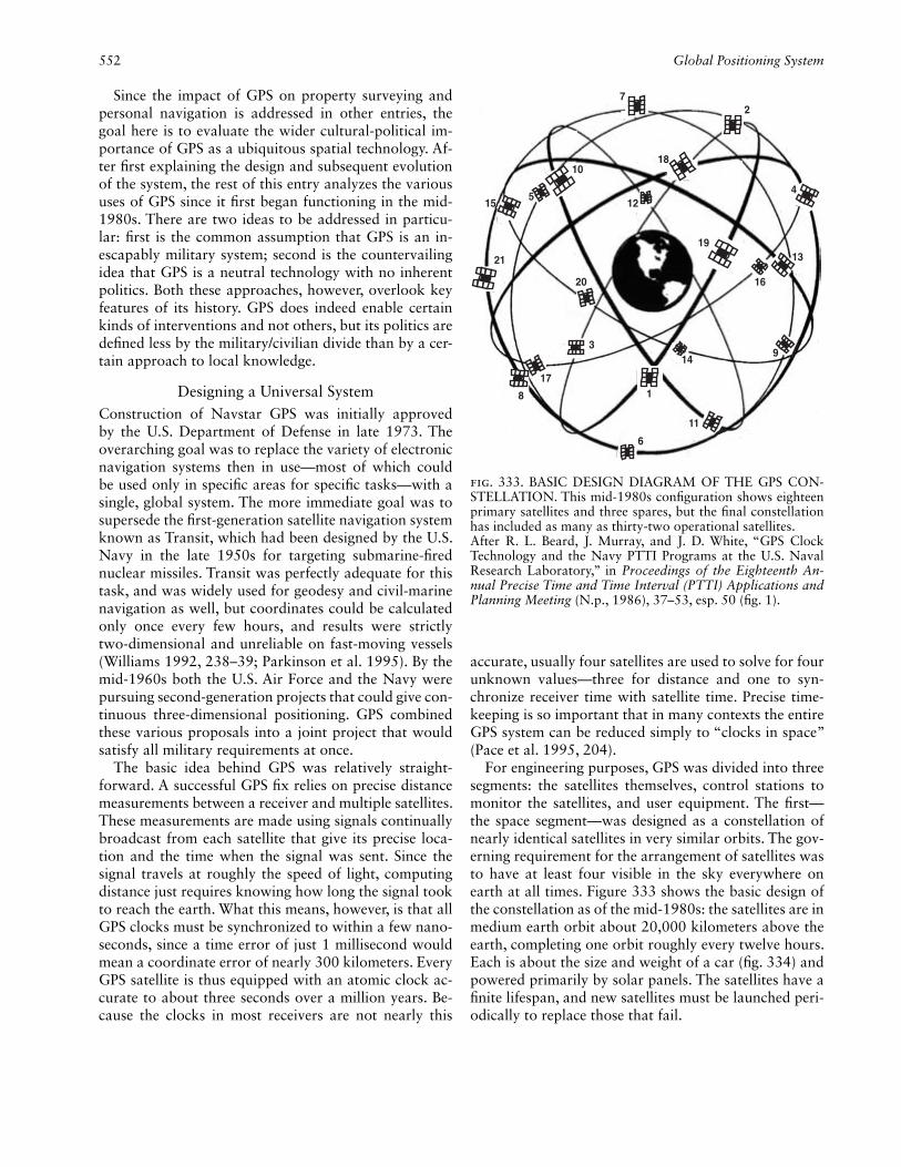
552 Global Positioning System

Since the impact of GPS on property surveying and personal navigation is addressed in other entries, the goal here is to evaluate the wider cultural-political im-portance of GPS as a ubiquitous spatial technology. Af-ter fi rst explaining the design and subsequent evolution of the system, the rest of this entry analyzes the various uses of GPS since it fi rst began functioning in the mid-1980s. There are two ideas to be addressed in particu-lar: fi rst is the common assumption that GPS is an in-escapably military system; second is the countervailing idea that GPS is a neutral technology with no inherent politics. Both these approaches, however, overlook key features of its history. GPS does indeed enable certain kinds of interventions and not others, but its politics are defi ned less by the military/civilian divide than by a cer-tain approach to local knowledge.

Designing a Universal SystemConstruction of Navstar GPS was initially approved by the U.S. Department of Defense in late 1973. The overarching goal was to replace the variety of electronic navigation systems then in use—most of which could be used only in specifi c areas for specifi c tasks—with a single, global system. The more immediate goal was to supersede the fi rst-generation satellite navigation system known as Transit, which had been designed by the U.S. Navy in the late 1950s for targeting submarine-fi red nuclear missiles. Transit was perfectly adequate for this task, and was widely used for geodesy and civil-marine navigation as well, but coordinates could be calculated only once every few hours, and results were strictly two-dimensional and unreliable on fast-moving vessels (Williams 1992, 238–39; Parkinson et al. 1995). By the mid-1960s both the U.S. Air Force and the Navy were pursuing second-generation projects that could give con-tinuous three-dimensional positioning. GPS combined these various proposals into a joint project that would satisfy all military requirements at once.

The basic idea behind GPS was relatively straight-forward. A successful GPS fi x relies on precise distance measurements between a receiver and multiple satellites. These measurements are made using signals continually broadcast from each satellite that give its precise loca-tion and the time when the signal was sent. Since the signal travels at roughly the speed of light, computing distance just requires knowing how long the signal took to reach the earth. What this means, however, is that all GPS clocks must be synchronized to within a few nano-seconds, since a time error of just 1 millisecond would mean a coordinate error of nearly 300 kilometers. Every GPS satellite is thus equipped with an atomic clock ac-curate to about three seconds over a million years. Be-cause the clocks in most receivers are not nearly this

accurate, usually four satellites are used to solve for four unknown values—three for distance and one to syn-chronize receiver time with satellite time. Precise time-keeping is so important that in many contexts the entire GPS system can be reduced simply to “clocks in space” (Pace et al. 1995, 204).

For engineering purposes, GPS was divided into three segments: the satellites themselves, control stations to monitor the satellites, and user equipment. The fi rst—the space segment—was designed as a constellation of nearly identical satellites in very similar orbits. The gov-erning requirement for the arrangement of satellites was to have at least four visible in the sky everywhere on earth at all times. Figure 333 shows the basic design of the constellation as of the mid-1980s: the satellites are in medium earth orbit about 20,000 kilometers above the earth, completing one orbit roughly every twelve hours. Each is about the size and weight of a car (fi g. 334) and powered primarily by solar panels. The satellites have a fi nite lifespan, and new satellites must be launched peri-odically to replace those that fail.

1

515

21

20

3

17

8

2

18

4

16

914

11

6

10

19

12

13

7

Fig. 333. BASIC DESIGN DIAGRAM OF THE GPS CON-STELLATION. This mid-1980s confi guration shows eighteen primary satellites and three spares, but the fi nal constellation has included as many as thirty-two operational satellites.After R. L. Beard, J. Murray, and J. D. White, “GPS Clock Technology and the Navy PTTI Programs at the U.S. Naval Research Laboratory,” in Proceedings of the Eighteenth An-nual Precise Time and Time Interval (PTTI) Applications and Planning Meeting (N.p., 1986), 37–53, esp. 50 (fi g. 1).

Global Positioning System 553

The control segment is composed of a number of fi xed receiver stations that track the satellites as they pass overhead. These stations are crucial for ensuring the reli-ability of GPS coordinates, since the accurate broadcast of each satellite’s location requires predicting how its orbit will be affected by factors like high-altitude gases and the earth’s gravity fi eld, and these predictions are not always correct. Actual measured satellite paths are thus continually processed to give new orbit-prediction data, which are subsequently uploaded to each satellite along with ongoing clock synchronization. In the Cold War–era 1970s, the main consideration for siting ground stations was that together they should provide as much tracking coverage as possible while still being located on U.S. military bases (fi g. 335).

Finally, the user equipment segment was designed to include a great variety of receivers, from multiantenna sets built into aircraft to portable receivers powered by batteries. The most important engineering distinction was between military and civilian equipment. Civilian uses were taken into account from the beginning (and were crucial for maintaining adequate funding from the U.S. Congress), but the military wanted to be able to deny GPS to unfriendly forces if necessary and to re-strict the use of GPS for high-accuracy targeting. GPS satellites were thus designed to transmit signals on two frequencies at once, one of which is encrypted for mili-tary use. Not only could the civilian signal be turned off in wartime, but access to both signals also enables direct correction of the effects of the earth’s ionosphere, thereby giving authorized users an accuracy advantage.

Given how closely these parts are interrelated, it is

diffi cult to identify any single feature that sets GPS apart from earlier systems, and apportioning credit for its design has been controversial. The main contest has been between two leaders of proto-GPS projects from the 1960s. The leader of the Navy’s Timation project, Roger L. Easton, has argued that “the GPS invention” was using space-based atomic clocks to measure distance (Easton 2005). In contrast, the director of the Air Force’s Project 621B, Bradford W. Parkinson, who subsequently went on to lead GPS in the 1970s, has instead identifi ed the GPS signal structure—an early use of a code division multiple access (CDMA) signal—as the “keystone tech-nology” (Parkinson and Powers 2010, 31). Not surpris-ingly, these are exactly the technologies that had been pursued by the Navy and the Air Force, respectively. Easton and Parkinson have both been awarded medals as the “inventor” or “father” of GPS, but the intracta-bility of their dispute over its key innovation suggests that assigning a defi nite inventor is not a useful exer-cise. GPS was a synthetic project both technologically and bureaucratically, and GPS-like ideas can be found in both satellite and terrestrial precedents as early as World War II. The creation of GPS, like most complex technical systems, was more a question of engineering and project management than groundbreaking novelty.

Since the initial design of the system in the early 1970s, most of its basic features have changed only slightly. GPS satellites, for example, have been made more robust, and the constellation has been tweaked in response to budget fl uctuations. Similarly, beginning in 2005 several new ground stations, generally sited on non-U.S. land, were added to the tracking network to allow constant monitoring by at least three receivers simultaneously. GPS signals have likewise been modifi ed as policies for civilian and military capabilities have changed. After discovering that early civilian receivers were more ac-curate than expected, the military began intentionally degrading the civilian signal. But this practice—known as Selective Availability—was discontinued in 2000, and later satellites were designed to broadcast using addi-tional frequencies to improve both civilian and military accuracy alike (Lazar 2002).

The combined effect of these changes, however, has been relatively minor compared to the impact of the radical miniaturization and falling price of user equip-ment. Figure 336, for example, shows the change in the size of portable military receivers between 1978 and 2004. Not only did they become smaller and lighter, but the later equipment also began displaying electronic maps rather than just raw coordinates. Civilian receiv-ers likewise transformed from specialist instruments to mass-market commodities complete with small color map display screens and up-to-date digital maps. The

Fig. 334. TESTING A BLOCK II GPS SATELLITE, 1985. The size of the satellite is indicated by the person standing lower right.Image courtesy of the Arnold Engineering Development Cen-ter, Arnold Air Force Base.

U.S. Air Force ground stations (shaded area shows tracking coverage)Additional tracking stations added after 2005 (operated by the United States, but mostly in foreign territory)Example ground track of an orbiting satellite (shifted east or west for other satellites)

Ascension DiegoGarcia

Kwajalein

CapeCanaveral

Master Control:Schriever Air Force Base

Hawaii

n o c o v e r a g e

Fig. 335. MAP OF GPS TRACKING STATIONS. Uniform global GPS coordinates still rely on the particular political-physical geography of the earth, since satellites must be con-tinually monitored from a network of ground stations.

Image courtesy of William J. Rankin.

Fig. 336. GPS RECEIVERS IN THE FIELD, CA. 1978. In 1973 the designers of GPS had hoped to eventually produce a portable military receiver weighing less than twelve pounds (5.5 kg). The Manpack of 1978 (left) weighed 14 kilograms, while the De-fense Advanced GPS Receiver (DAGR) of 2004 (right) weighed about 400 grams and fi t comfortably in the hand.

Left, from Lazar 2002, 45; permission courtesy of the Aero-space Corporation, Los Angeles. Right, image courtesy of the National Museum of American History, Smithsonian Institu-tion, Washington, D.C.

Global Positioning System 555

cost of an entry-level receiver fell from $1,000 to $100 between 1992 and 1997, and the smallest receiver in the early 2000s was the size of a wristwatch (fi g. 337). Even the most optimistic predictions in the 1980s for the diffusion of GPS turned out to be far too conserva-tive (Kumar and Moore 2002, 69, 79).

This ubiquity has had a profound effect on the way GPS has been understood. Rather than being seen just as a positioning and navigation technology, beginning in the mid-1990s GPS began to be described as new kind of public utility, alongside electricity, gas, and water (Pace et al. 1995, 184). The product to be delivered was loca-tion, and the marginal cost was essentially zero. One of the most common analogies was between GPS and the Internet, as both were sponsored by the U.S. military and eventually transformed into open platforms (Aporta and Higgs 2005). The basic idea here was that forecast-ing GPS’s future uses—or even providing a comprehen-sive list of current ones—became essentially impossible. More conceptually, however, the larger implication was that GPS should not be seen as simply a tool for mak-ing geographic space legible. Rather, GPS became a re-placement for traditional space (and time) altogether. Both the spaces of day-to-day experience and the spaces constructed by representational maps were superseded by a space that was more immediately calculable, less

historical, and almost perfectly uniform (Kurgan 1994; Rankin 2011).

The Uses (and Abuses) of GPSThe history of GPS after it fi rst became operational is largely a history of how it has been used. The major trends are relatively clear: civilian applications quickly outnumbered military uses, and GPS became tightly integrated into other systems of communication and geographic management. Evaluating the impact of these trends, however, is less straightforward, as the social consequences of GPS have been wide-ranging, often un-anticipated, and at times contradictory. The recent his-tory of GPS thus raises questions relevant to any history of infrastructure: With the transformation of GPS into a multiuse utility, what is gained and what is lost? Who wins and who loses? Two issues are especially important here: the relationship between civilian GPS and its mili-tary origins and the politics of action at a distance.

Two of the most signifi cant early uses of GPS were in cartography and war. The surveying industry began to adopt GPS in the mid-1980s while the constellation was still incomplete. Its effect was profound. GPS not only solidifi ed the decades-long transition from traditional astronomical and angular methods to black-box elec-tronic equipment, but it further untethered surveying from the geography of national states. The widespread use of the GPS world datum (WGS84) enabled every-thing from cross-border engineering projects to reliable measurement in international waters, and it became a de facto standard for global geographic information systems (GIS) platforms. More broadly, GPS signaled a shift in the very nature of mapping. As the tools of map-ping merged with the tools of navigation, it became in-creasingly diffi cult to distinguish mapmaking from map use. The famous tales by Lewis Carroll and Jorge Luis Borges about maps on the same scale as the territory thus apply quite well to GPS, since using GPS for fi shing management, offshore drilling, or coordinating archaeo-logical sites is effectively mapping at a scale of 1:1. GPS is used both to make a record of important points and to return to them; traditional mapping problems of se-lection and representation need not arise at all (Rankin 2011, 440–51).

The impact of GPS on military strategy was no less decisive. During the Persian Gulf War, GPS lowered the cost of precision bombing and enabled large-scale troop coordination in the featureless Iraqi desert, both of which gave the U.S. a substantial advantage. After the war GPS quickly became a core component of a “precision revolution” in American strategy that priori-tized smaller, more mobile, and more technologically ad-vanced forces. GPS also changed the geography of war,

Fig. 337. FIRST GPS WRISTWATCH, PRO TREK. Sold by Casio in 1999 for $895; ten years later GPS watches were no larger than their non-GPS counterparts and cost just over $100.Size of the watch body: 6.5 × 6.5 cm.

556 Global Positioning System

since GPS-guided missiles and bombers can be launched thousands of miles from their target. The dream—unre-alized, to be sure—is to remove soldiers from the battle-fi eld altogether (Rip and Hasik 2002).

The multiplication of civilian GPS applications in the 1990s and 2000s largely followed these precedents of automation and tighter geographic coordination, but the mass commercialization of GPS also raised entirely new issues. Most of the best-known uses of GPS had been under development since the early 1980s, such as automobile and aircraft navigation, close control of farm equipment for precision agriculture, or the direct measurement of tectonic plate drift. The use of GPS for time synchronization—in cell phone networks, power grids, or even municipal stoplights—also extended ear-lier techniques. But in the late 1990s several applications began to proliferate that had not been anticipated and did not sit easily within traditional descriptions of GPS as a positioning, navigation, and timing (PNT) system. Foremost among these was the use of GPS for tracking (of wildlife, criminals, children, or cargo) and amateur mapping by artists and activists. These applications have provoked the most debates about the nature of GPS, raising questions of civil liberties, privacy, and the de-mocratization of cartography.

There have been primarily two ways that scholars have interpreted the spread of civilian GPS. First is a pessimistic assumption that GPS is an inherently mili-tary technology and that its widespread use represents the militarization of civil society. The strongest versions of this argument claim that GPS (along with its cousin, GIS) has created a cultural obsession with precision so

pervasive that techniques of military targeting end up blending seamlessly into practices like targeted mar-keting. Not only has GPS turned American consumers into “militarized subjects” (Kaplan 2006, 708), but the integration of GPS into everything from cell phones to traditional hunting practices will “deliver American militarized realities” abroad as well (Mark H. Palmer and Robert Rundstrom in Aporta and Higgs 2005, 748). A less forceful version of this interpretation also drove much of the debate in the early 2000s about compe-tition between GPS and the European Union’s civilian (and partly commercial) Galileo system. Many observ-ers, from American pundits to foreign heads of state, distrusted claims that a system maintained by the U.S. military would remain reliably accessible, despite high-level assurances (Han 2008).

The second interpretation—often explicitly opposed to the fi rst—instead posits GPS, and technology in gen-eral, as an inherently neutral tool that can be used either for good or for evil, regardless of its origins. Optimis-tic scholars tend to emphasize the usefulness of GPS for things like tracking endangered species, clearing land-mines, or the rapid mapping of Haiti after the 2010 earthquake (fi g. 338). Optimists also stress that although GPS can be used for top-down surveillance by police or employers, it can also be used for bottom-up “sousveil-lance” to hold governments accountable, such as when marginalized citizens use GPS for reporting broken street lights in New Jersey or mapping informal settlements in Kenya. Even advanced missile guidance has its good side, since surgical strikes on infrastructure obviate the senseless killing of area bombing (Klinkenberg 2007).

Fig. 338. RAPID HUMANITARIAN RESPONSE USING GPS. Coverage of Port-au-Prince, Haiti, by the collaborative project OpenStreetMap before (left) and two days after (right) the 2010 earthquake.

Image courtesy of William J. Rankin.

Global Positioning System 557

Belief in technological neutrality also under girds certain kinds of pessimism as well. Jerome E. Dobson and Pe-ter F. Fisher, for example, have issued strong warnings about the coming mass-surveillance society and the po-tential for a new “geoslavery” enabled by coercive GPS tracking. For them, the worry is not the military, or even GPS itself, but its exploitation by unscrupulous corpora-tions and individuals; arguing that technology is neutral is important rhetorically for defending GPS against these abuses (Dobson and Fisher 2007; Herbert 2006).

There are good reasons to challenge military essen-tialism. Claiming that technology is inherently neutral, however, is no less problematic. Certainly, the assump-tion that military-sponsored technology can only fur-ther militarist goals is empirically unfounded. Yet it is also true that every technology is inevitably designed for certain tasks and not others and therefore is prejudiced with specifi c capabilities and constraints. Technological systems are also always being modifi ed to further privi-lege some uses over others. Military pessimists tend to simplify this history to confi rm their suspicions; tech-nological neutralists, however, tend to overlook it alto-gether. Neutralism can also be rather fatalist. Saying that technology inevitably has both positive and negative so-cial effects can easily imply that any attempt to steer the course of technological progress will prove futile.

For GPS, both its initial design and its ongoing evolu-tion suggest that a different interpretation is necessary. First, GPS was explicitly designed so that it could serve more than just military interests. One of the basic mili-tary requirements in the late 1960s was that it use only one-way broadcast from satellites to users rather than two-way communication. The latter would have been technologically simpler, but any ground transmission could be used by the enemy for tracking and targeting. For this reason, civilian agencies—especially the Federal Aviation Administration and the National Aeronautics and Space Administration (NASA)—initially expressed little interest in GPS and instead proposed systems that would broadcast users’ locations back to a satellite to enable active air traffi c control or ship monitoring. These systems also would have only supported a lim-ited number of receivers at once (Stansell 1971, 107). In other words, it was precisely the involvement of the military—and its lack of neutrality—that made GPS an open system that could support unlimited nonmilitary users, with features like privacy and anonymity priori-tized over tracking and surveillance.

Second, by the early 2000s the military had decisively lost much of its control over GPS, after a long struggle with civilian agencies and corporations. Not only had President Bill Clinton annulled the military’s Selective Availability policy, but the governance of GPS was changed so that top-level responsibility was shared be-

tween the Departments of Defense and Transportation. Even more important was the civilian development of local and regional augmentation systems to increase ac-curacy and reliability (fi g. 339). These systems had effec-tively thwarted Selective Availability in the 1990s, and because they were used for life-critical applications like harbor and air navigation, they likewise drastically re-duced the military’s ability to disable the civilian signal in wartime (Pace et al. 1995, 20–27). The very existence of these ongoing technological and policy changes make it diffi cult to see GPS as neutral, and again military in-terests tended to align with individual privacy, since similar augmentation systems have enabled some of the most Orwellian GPS applications, such as indoor track-ing (Trimble 2003).

If GPS is neither inherently militaristic nor inherently neutral, what is it? The answer need not be so grandi-ose. The key conceptual feature of GPS is that it replaces lumpy, historical, human space with a globally uniform mathematical system. By extension, the central political fact about GPS is that it substitutes a locally available grid of geographic coordinates for other kinds of local knowledge and encourages intervention without local commitment. This intervention can be initiated from afar— precision bombing, humanitarian relief, GPS track-ing—or it can be projected outward, as with activist map-ping. In all cases, however, the goal is to encourage action and to bridge the political divide between center and pe-riphery. This has been the goal of most offi cial mapping from the sixteenth century forward, but the relationships GPS constructs are much less mediated, since GPS is not a technology of representation. GPS can also be wielded by almost anyone, not just institutions with massive re-sources. The relevant political distinction is therefore not between state and nonstate, military and civilian, or even good and bad, but between local and nonlocal decision making. And thus with GPS the basic political question, as ever, is not what or how, but by whom.

William J. Rankin

See also: Cold War; Cruise Missile; Geodesy: Satellite Geodesy; Hy-drographic Techniques: Global Positioning System in Hydrographic Mapping; Property Mapping Practices: Global Positioning System and Property Surveying; Warfare and Cartography; Wayfi nding and Travel Maps: In-Vehicle Navigation System

Bibliography:Aporta, Claudio, and Eric Higgs. 2005. “Satellite Culture: Global Po-

sitioning Systems, Inuit Wayfi nding, and the Need for a New Ac-count of Technology.” Current Anthropology 46:729–53.

Dobson, Jerome E., and Peter F. Fisher. 2007. “The Panopticon’s Changing Geography.” Geographical Review 97:307–23.

Easton, Richard. 2010. Response to Bradford W. Parkinson. Inside GNSS 5, no. 3:15–17.

Easton, Roger L. 2005. “GPS Inventor.” Memoir. Online publication.Han, Sang Wook Daniel. 2008. “Global Administrative Law: Global

Governance of the Global Positioning System and Galileo.” ILSA Journal of International & Comparative Law 14:571–93.

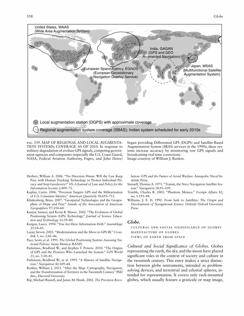
558 Globe

Herbert, William A. 2006. “No Direction Home: Will the Law Keep Pace with Human Tracking Technology to Protect Individual Pri-vacy and Stop Geoslavery?” I/S: A Journal of Law and Policy for the Information Society 2:409–73.

Kaplan, Caren. 2006. “Precision Targets: GPS and the Militarization of U.S. Consumer Identity.” American Quarterly 58:693–713.

Klinkenberg, Brian. 2007. “Geospatial Technologies and the Geogra-phies of Hope and Fear.” Annals of the Association of American Geographers 97:350–60.

Kumar, Sameer, and Kevin B. Moore. 2002. “The Evolution of Global Positioning System (GPS) Technology.” Journal of Science Educa-tion and Technology 11:59–80.

Kurgan, Laura. 1994. “You Are Here: Information Drift.” Assemblage 25:14–43.

Lazar, Steven. 2002. “Modernization and the Move to GPS III.” Cross-link 3, no. 2:42–46.

Pace, Scott, et al. 1995. The Global Positioning System: Assessing Na-tional Policies. Santa Monica: RAND.

Parkinson, Bradford W., and Stephen T. Powers. 2010. “The Origins of GPS and the Pioneers Who Launched the System.” GPS World 21, no. 5:30–41.

Parkinson, Bradford W., et al. 1995. “A History of Satellite Naviga-tion.” Navigation 42:109–64.

Rankin, William J. 2011. “After the Map: Cartography, Navigation, and the Transformation of Territory in the Twentieth Century.” PhD diss., Harvard University.

Rip, Michael Russell, and James M. Hasik. 2002. The Precision Revo-

lution: GPS and the Future of Aerial Warfare. Annapolis: Naval In-stitute Press.

Stansell, Thomas A. 1971. “Transit, the Navy Navigation Satellite Sys-tem.” Navigation 18:93–109.

Trimble, Charles R. 2003. “Phantom Menace.” Foreign Affairs 82, no. 5:193–94.

Williams, J. E. D. 1992. From Sails to Satellites: The Origin and Development of Navigational Science. Oxford: Oxford University Press.

Globe.Cultural and Social Significance of GlobesManufacture of GlobesViews of Earth from Space

Cultural and Social Signifi cance of Globes. Globes representing the earth, the sky, and the moon have played signifi cant roles in the context of society and culture in the twentieth century. This entry makes a strict distinc-tion between globe instruments, intended as problem-solving devices, and terrestrial and celestial spheres, in-tended for representation. It covers only rack-mounted globes, which usually feature a graticule or map image,

United States, WAAS(Wide Area Augmentation System)

European Space Agency, EGNOS

India, GAGAN(GPS and GEO

Augmented Navigation)

(Multifunctional Satellite Augmentation System)

Japan, MSAS

Local augmentation station (DGPS) with approximate coverage

Regional augmentation system coverage (SBAS); Indian system scheduled for early 2010s

(European Geostationary Navigation Overlay Service)

Fig. 339. MAP OF REGIONAL AND LOCAL AUGMENTA-TION SYSTEMS; COVERAGE AS OF 2010. In response to military degradation of civilian GPS signals, competing govern-ment agencies and companies (especially the U.S. Coast Guard, NASA, Federal Aviation Authority, Fugro, and John Deere)

began providing Differential GPS (DGPS) and Satellite-Based Augmentation System (SBAS) services in the 1990s; these sys-tems increase accuracy by monitoring raw GPS signals and broadcasting real-time corrections.Image courtesy of William J. Rankin.

Globe 559

as well as their two-dimensional and three-dimensional reproductions.

In addition to their role as scientifi c instruments and teachings aids, terrestrial and celestial globes have long been important as symbols and signs. In pictures as well as three-dimensional spherical models, globes have been an integral part of the allegorical language of Western culture: the terrestrial globe as a symbol of the earthly and the ephemeral and the celestial globe as a symbol of the cosmos, the infi nite universe, the eternal, and the divine. In these roles, globes have not only symbolized the power, status, and wealth of sovereigns and world leaders but also represented the knowledge and profes-sionalism of geographers, cartographers, mapmakers, astronomers, navigators, explorers, and world travelers.

In the twentieth century, geopolitics and economic glob alization further enhanced the signifi cance of terres-trial globes. While the traditional symbolism of globes was apparent throughout the century, the sociocultural context was in fl ux. As the importance of globes as sci-entifi c instruments declined, their symbolic meaning changed as well, particularly for terrestrial globes (in-cluding reproductions and replicas), as the globe became largely a sign of global activity, open-mindedness, or in-terest in science and education. And around midcentury a new meaning emerged when the terrestrial globe be-came a symbol of world peace.

Because of a dearth of relevant scholarly studies, in-sights into the cultural and social signifi cance of globes must rely heavily on indirect or less formal sources, including scholarly research on globes as commercial products, analyses of globe producers’ advertisements and promotional literature, and essays on globes dis-played publicly in lobbies, plazas, and other public set-tings. In addition to studies of the role and meaning of two-dimensional and three-dimensional reproductions and replicas of globes in diverse contexts, further evi-dence for the social importance of globes can be found in dictionaries and encyclopedias. Indeed, the words “globe” and “global” embody much of the cultural sig-nifi cance of globes in the twentieth century.

The importance of globes in the sociocultural con-text of the twentieth century is closely associated with their visibility—in particular, as representational objects linked in the public’s imagination to important person-alities and institutions—as well as with the globe’s im-portance as a commercial product. After all, the greater the number of globes produced and disseminated, the greater their role in culture and society, and the greater the impact of reproductions and replicas of globes as symbols and signs.

In the late nineteenth and early twentieth centuries, globe instruments, especially terrestrial globes, were pri-marily used as teaching tools in schools and as deco-

rative accessories in private and semiprivate living and work areas (fi g. 340). Indeed, in schools and colleges as well as in better-educated middle-class households, the globe was as commonplace as an encyclopedia or a world atlas. During that period, globes were also used as furnishings in dollhouses, and manufacturers who of-fered a wide range of globe products expressly adver-tised their smallest versions as “dollhouse globes.”

During the fi rst half of the century a huge number of globe instruments, especially terrestrial globes, were manufactured in Europe and the United States. Pro-ducers in the United States successfully counteracted the standardized and inexpressive map images of these mass-produced instruments by making a variety of ver-sions, differentiated by mounts ranging from the simple to the highly elaborate.

Terrestrial globes attained their greatest importance in society and geopolitics in the 1930s with the devel-opment, production, and marketing of the elaborately designed Großglobus für Staats- und Wirtschaftsführer (large globe for state and business leaders), produced in different representative mount variations by the Berlin-based Columbus-Verlag Paul Oestergaard. These globes were as large as 106 centimeters in diameter and attained a total height of 165 or 175 centimeters, depending on the size of the mount.

During the second half of the century, the importance of globes as educational tools declined and by century’s end was almost negligible. This decline—understandable insofar as the globe was now perceived as an expensive, bulky version of a minimally detailed small-scale world map—had a direct impact on the role of globes as suc-cessful commercial products. As a result, a marked re-duction in the number of globes produced went hand in hand with the consolidation of manufacturing fi rms, and the relevance of globes (including reproductions and replicas) as symbols and signs in the societal con-text diminished as well. Even so, electronic technology introduced other scientifi c tools and media, such as car-tographic animations and the interactive virtual globe, which had symbolic meaning and perpetuated the no-tion of the globe as a sociocultural concept. Despite this diminished sociocultural importance, two-dimensional images of globes had become increasingly prominent on posters, stamps, poster stamps, bookplates, coins, banknotes, securities, and corporate logos, while three-dimensional reconstructions served a symbolic function, particularly in public places.

During the second half of the nineteenth century and the fi rst half of the twentieth century, huge globes were mounted atop or adjacent to important buildings such as railway stations, post offi ces, telegraph offi ces, hotels, department stores, travel agencies, newspaper publishers, and chambers of industry and commerce.

Fig. 340. DECORATE YOUR HOME WITH COLUM-BUS TERRESTRIAL GLOBES, CA. 1935. Advertisement in a brochure of the Berlin-based Columbus-Verlag Paul Oestergaard for globes as home and offi ce furniture. Top: rack-mounted globe, 50-centimeter diameter; bottom: table

globe, 34- centimeter diameter. From Jubiläumskatalog (Berlin: Columbus-Verlag, 1934), 14. Image courtesy of Jan Mokre. Permission courtesy of Columbus Verlag Paul Oestergaard, Krauchenwies.

Globe 561

Additionally, globes were added as three-dimensional elements to sculptures, monuments, and tombs, particu-larly those commemorating cartographers, astronomers, navigators, and world travelers.

Huge globes were often erected at world exhibitions and other venues where size was an emblem of achieve-ment. The 1900 Paris Exposition Universelle featured a 140-foot-diameter celestial globe accessible from the inside (fi g. 341), and the 1964–65 New York World’s Fair at Flushing Meadows Park included a twelve-story steel terrestrial globe. In the United States in particular,

large globes have been placed in the lobbies of presti-gious newspaper offi ces and prominent railway stations and airports. Babson College (renamed from Babson In-stitute in 1969), a business-oriented college in Wellesley, Massachusetts, is known locally for its 28-foot-diameter outdoor globe, built in the mid-1950s by founder Roger Ward Babson. The structure had deteriorated by the late 1980s, but when administrators announced plans to tear it down, outraged alumni raised funds for its restoration, completed in 1993 (fi g. 342). In 1998 the DeLorme Company unveiled a 41.5-foot-diameter in-door globe adjacent to its factory and map store in Yar-mouth, Maine. Nicknamed Eartha, the Guinness Book of Records (2001) proclaimed the DeLorme globe as the world’s biggest revolving globe. Despite the globe’s de-creased presence in homes and classrooms, these exam-ples as well as the recurrent use of globes in advertising highlight the continued cultural importance of globes the twentieth century.

Three distinctly twentieth-century phenomena ran counter to the declining cultural and social signifi cance of the globe. First, prominent people from diverse sec-tors of society were photographed with globes. There exist, for example, several portraits of U.S. President Theodore Roosevelt during his presidential terms (1901–9) with a large terrestrial globe (almost 80 cm diameter), perhaps taken in view of his active foreign policies (fi g. 343). Second, globes appeared in feature fi lms and television dramas as furnishings in middle-class homes much more commonly than in reality, even at the end of the century. The traditional popularity of globes as symbols of learning and affl uence survived in the fantasies of mass media set designers. Third, lu-nar globes achieved a brief prominence from the early 1960s through the early 1970s, when the United States and the Soviet Union faced off in an epic race to the moon. Within a short time, manufacturers were produc-ing large quantities of lunar globes—scientifi c and com-mercial—as well as similarly shaped tin toys, souvenirs, money boxes, and other knickknacks. These attracted great interest: for the fi rst time, the cartographic rep-resentation of the backside of the moon was possible, and the landing sites of planned and successful space expeditions were represented on lunar globes. Offi cial photographs from the National Aeronautics and Space Administration (NASA) often juxtaposed American as-tronauts and lunar globes (fi g. 344).

Virtual globes based on digital data and programming emerged in the fi nal decade of the twentieth century fol-lowing the development of the digital world atlas, itself a refl ection of slightly earlier advances in interactive graph-ics and personal computing as well as the development of massive worldwide data sets, including environmental and historical data. The user could rotate a two-dimen-

Fig. 341. LE GRAND GLOBE CÉLESTE AT THE EXPOSI-TION UNIVERSELLE IN PARIS, 1900. The huge celestial globe had a diameter of 46 meters and rested on a construction of four masonry piers. Inside it was a second celestial globe with a diameter of 36 meters, and within that globe was a ter-restrial globe with a diameter of 8 meters. Visitors could pay an additional fee and, using a spiral staircase in the terrestrial globe, climb up to the North Pole and look at the sky, which was painted on the inside of the second celestial globe.Image courtesy of the Brooklyn Museum Archives, Goodyear Archival Collection.

562 Globe

sional image of a globe to any position and then zoom in so that the horizon was no longer visible, while the projected globe became merely a projected map.

Despite the diminished importance of contemporary globes, old globes enjoyed increased interest as collec-tor’s items, as refl ected in sales and auction catalogs, their presence in major public and private collections, and an increase in scientifi c studies on globes. Particu-larly signifi cant was the emergence of a scholarly institu-tion focused on globes. The International Coronelli Soci-ety for the Study of Globes, founded in Vienna in 1952, has fostered the scientifi c study of globes as a distinct cartographic expression, and its journal Der Globus-freund: Wissenschaftliche Zeitschrift für Globenkunde, initiated the same year, provided an outlet for scholarly papers on globes, their producers, and their signifi cance. An English-language version, Globe Studies: The Jour nal of the International Coronelli Society, began in 2002.

Jan Mokre

See also: Colonial and Imperial Cartography; Projections: Cultural and Social Signifi cance of Map Projections; Visualization and Maps

Bibliography:Fisher, Irving, and O. M. Miller. 1944. World Maps and Globes. New

York: Essential Books.Lehmann, René. 1999. “Der Columbus-Großglobus für Staats- und

Wirtschaftsführer.” Mitteilungen: Freundeskreis für Cartographica in der Stiftung Preussischer Kulturbesitz e.V. 13:33–36.

Meine, Karl-Heinz. 1969–71. “Die Stellung des Globus in den Wissen-schaften—früher und heute.” Der Globusfreund 18–20:100–107.

Mokre, Jan. 1997. “Immensum in parvo—Der Globus als Symbol.” In Modelle der Welt: Erd- und Himmelsgloben, ed. Peter E. Allmayer-Beck, 70–87. Vienna: Bibliophile Edition.

———. 1999. “Globen unter freiem Himmel: Beispiele aus Wien.” Der Globusfreund 47–48:125–41.

———. 2008. Rund um den Globus: Über Erd- und Himmelsgloben und ihre Darstellungen. Ed. Peter E. Allmayer-Beck. Vienna: Biblio-phile Edition.

Muris, Oswald, and Gert Saarmann. 1961. Der Globus im Wandel der Zeiten: Eine Geschichte der Globen. Berlin: Columbus Verlag Paul Oestergaard.

Riedl, Andreas. 2007. “Digital Globes.” In Multimedia Cartography,

Fig. 342. THE BABSON WORLD GLOBE. George C. Izenour designed the enormous globe, with a diameter of 28 feet. The idea came from Roger Ward Babson’s grandson, Roger Web-ber. It was erected on the campus of the Babson Institute and dedicated in 1955. The sphere, which rotates using a motor, is

made of steel with enameled steel panels fastened on it; they represent the earth’s surface in twenty different colors. Photo-graph 2005.Image courtesy of Babson College, Babson Park.

Globe 563

2d ed., ed. William Cartwright, Michael P. Peterson, and Georg F. Gartner, 255–66. Berlin: Springer.

Robinson, Arthur H. 1997. “The President’s Globe.” Imago Mundi 49:143–52.

Manufacture of Globes. During the twentieth century, globemakers in Europe and the United States produced conventional terrestrial and celestial globes as well as replicas of Mars, Venus, Mercury, and Earth’s moon. This entry focuses on the serial, or mass-market, pro-duction of globes that adhere to a discernible scientifi c standard. It thus ignores metal toys or globe puzzles as well as single-piece globes crafted individually for a spe-cifi c client or special purpose.

At the beginning of the twentieth century, globes were produced by gluing together two hollow papier-mâché hemispheres. A gypsum-like paste was applied to the sur-face of the sphere and sanded down after drying. Then a world map, which was reproduced lithographically and typically consisted of twelve spherical bi-angles and two polar caps, was glued or laminated onto the sphere. Subsequently, the globe was covered with a protective coating and equipped with an axis.

Because globes had already lost their standing as sci-entifi c instruments by the middle of the nineteenth cen-tury, manufacturers did not bother to fully outfi t globes with a horizontal circle, meridian circle, altitude quad-rant, hour hand, and compass. Instead, they mounted the globe on a simple frame, typically consisting of a base plate and a center column. In many cases, the globe was fi tted with a metal meridian circle that featured de-gree counts or with a half meridian circle.

Beginning in the 1910s, the manufacture of hollow hemispheres was shifted to hydraulic presses, which produced very smooth surfaces and made the gypsum layer obsolete. The world map was now directly lami-nated onto a cardboard sphere. Gradually, more modern and effi cient industrial reproduction methods replaced lithographic map printing.

In the 1930s, some manufacturers in the United States implemented a mechanical, hydro-press method for pro-ducing cardboard globes. This method glued maps with a special projection screen for the northern and south-ern hemispheres onto cardboard disks, which were then cut out mechanically to create surfaces shaped like pin-

Fig. 343. THEODORE ROOSEVELT, FULL-LENGTH POR-TRAIT, WITH LARGE GLOBE IN THE BACKGROUND, AT THE WHITE HOUSE IN 1903.Image courtesy of the Library of Congress, Prints and Photo-graphs Division, Washington, D.C.

Fig. 344. ASTRONAUT JOHN W. YOUNG WITH A LUNAR GLOBE, 1971. Young, a participant in the U.S. space missions Gemini, Apollo, and the fi rst space shuttle, was the ninth man to walk on the moon as commander of Apollo 16 in 1972.Image courtesy of NASA/Johnson Space Center.

564 Globe

wheels, with sharply angled isosceles triangles meeting at the center (North or South Pole). These cardboard disks were then molded in a press, under intense heat and pres-sure, to produce hollow hydro-pressed hemispheres. The northern and southern hemispheres were then clipped at the edges, glued together to form a sphere, coated with a protective coating, and mounted on a frame.

In the 1920s globe manufacturers introduced trans-lucent globes illuminated by electricity. The world map was printed on transparent paper and glued or laminated onto a hand-blown, hollow glass sphere into which a light bulb was fi tted. This type of globe production ex-perienced a revolutionary improvement in the 1950s, when the globe map was printed on both sides using a complex procedure. Depending on whether or not the globe was illuminated, it showed either a physical or a political map.

From the 1950s onward globes were more commonly produced using plastic rather than glass, and by the end of the century plastic had largely displaced cardboard as the basic material for mass-produced globes. Three dif-ferent production methods were used for plastic globes. The simplest method followed the traditional approach of gluing segments of a map printed on paper or plastic fi lm onto a hollow plastic sphere. The second method required special map projections for the Northern and Southern Hemispheres; the maps were printed on cir-cular pieces of plastic fi lm, which were subjected to a thermoplastic process that combined thermoforming with injection molding and simultaneously produced Northern and Southern Hemispheres, which were then joined into complete a sphere (fi g. 345). A third produc-tion method entailed mechanically mounting fi lms with cartographic images onto previously molded hollow

plastic spheres. In addition to the traditional format, plastic globes were manufactured as illuminated globes, sometimes with changing images.

Relief globes were also manufactured in the twentieth century. Initially they were crafted by hand, the tradi-tional method, by modeling the terrain in a gypsum-like paste on the outside of a cardboard sphere with the vertical dimension typically exaggerated, sometimes for dramatic effect. From the 1940s onward, machine-shaped terrain segments were commonly glued onto a plastic sphere. In the second half of the twentieth cen-tury, earth-relief globes were produced using mechani-cally pressed hemispheres made of cardboard as well as plastic. The fi rst mass-produced earth-relief globe fea-turing both terrain and seabed profi les in three dimen-sions was introduced in 1990.

Magnetic levitation globes were introduced in the late 1980s. In this special design, a combination of perma-nent magnets and computer-controlled electromagnetic levitation keeps the globe in balance and rotates it about the axis. These globes represent the fi nal stage of devel-opment of analog globes.

A completely new development emerged toward the end of the twentieth century. Virtual globes based on digital data and computer software can be displayed on fl at or spherical screens, reproduced as holograms, or accessed interactively online. These three-dimensional models of the planet can show not only static or ani-mated representations of current patterns, such as sur-face weather, but also historical events, such as explora-tions, warfare, and boundary changes. When equipped with zoom-in and pan functions, virtual globes afford a seamless integration of the globe with intermediate- and large-scale maps.

Fig. 345. GLOBE PRODUCTION AT COLUMBUS-VERLAG. Globe hemispheres are produced by a combination of thermo-forming and injection molding. Hemisphere being removed from the machine (left) and stacked (right).

Image courtesy of Columbus-Verlag, Krauchenwies.

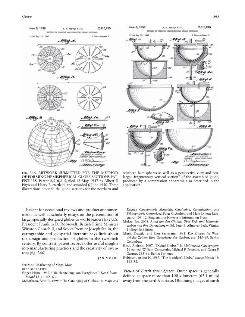
Globe 565

Except for occasional reviews and product announce-ments as well as scholarly essays on the presentation of large, specially designed globes to world leaders like U.S. President Franklin D. Roosevelt, British Prime Minister Winston Churchill, and Soviet Premier Joseph Stalin, the cartographic and geospatial literature says little about the design and production of globes in the twentieth century. By contrast, patent records offer useful insights into manufacturing practices and the creativity of inven-tors (fi g. 346).

Jan Mokre

See also: Marketing of Maps, MassBibliography:Finger, Heinz. 1967. “Die Herstellung von Plastgloben.” Der Globus-

freund 15–16:155–63.McEathron, Scott R. 1999. “The Cataloging of Globes.” In Maps and

Related Cartographic Materials: Cataloging, Classifi cation, and Bibliographic Control, ed. Paige G. Andrew and Mary Lynette Lars-gaard, 103–12. Binghamton: Hayworth Information Press.

Mokre, Jan. 2008. Rund um den Globus: Über Erd- und Himmels-globen und ihre Darstellungen. Ed. Peter E. Allmayer-Beck. Vienna: Bibliophile Edition.

Muris, Oswald, and Gert Saarmann. 1961. Der Globus im Wan-del der Zeiten: Eine Geschichte der Globen, esp. 245–69. Berlin: Columbus.

Riedl, Andreas. 2007. “Digital Globes.” In Multimedia Cartography, 2d ed., ed. William Cartwright, Michael P. Peterson, and Georg F. Gartner, 255–66. Berlin: Springer.

Robinson, Arthur H. 1997. “The President’s Globe.” Imago Mundi 49:143–52.

Views of Earth from Space. Outer space is generally defi ned as space more than 100 kilometers (62.1 miles) away from the earth’s surface. Obtaining images of earth

Fig. 346. ARTWORK SUBMITTED FOR THE METHOD OF FORMING HEMISPHERICAL GLOBE SECTIONS PAT-ENT. U.S. Patent 2,510,215, fi led 12 May 1947 by Albert F. Pityo and Harry Butterfi eld, and awarded 6 June 1950. These illustrations describe the globe sections for the northern and

southern hemispheres as well as a perspective view and “en-larged fragmentary vertical section” of the assembled globe, produced by a compression apparatus also described in the application.

566 Globe

from space in the twentieth century was a monumental conceptual and technological achievement. These im-ages provided unprecedented regional perspectives of land use/land cover and biophysical processes, and the related data resulted in new cartographic products, in-cluding detailed image maps of the earth and animations for processes as varied as tracking hurricanes, monitor-ing urban expansion, and measuring seasonal changes in biomass. In addition, geographic information about remote places on the planet became available.

The fi rst aerial photograph was taken by Gaspard-Félix Tournachon (known as Nadar) in 1858 from a tethered balloon only a few hundred meters above Petit Bicêtre, France (Colwell 1997, 6). In 1935, pho-tographs obtained from the Explorer II balloon at an unprecedented altitude of 22 kilometers (13.7 miles) documented the curvature of the earth. On 24 October 1946 the fi rst photograph of the earth from space was acquired by a 35 millimeter motion picture camera on-board an unmanned captured German V-2 rocket that attained an altitude of 104 kilometers (64.6 miles) but did not achieve orbit (fi g. 347) (Reichhardt 2006). Be-tween 1945 and 1950 cameras fl own on numerous V-2s captured useful regional cartographic information. In 1950 the engineer who developed the camera fl own on-board the V-2 rockets predicted in National Geographic that these types of images would become commonplace in mapping the earth’s surface (Holliday 1950, 512).

The Soviet Union’s successful launch of the Sputnik 1 satellite in October 1957 spurred an intensifi ed effort by the United States. The fi rst photograph of earth ac-quired by a U.S. satellite was collected by Explorer VI

on 14 August 1959. The fi rst crude television image of earth from an orbital platform was obtained by the TIROS 1 (Television Infrared Observation Satellite) on 1 April 1960. In 1960 the U.S. Central Intelligence Agen-cy’s Corona spy satellite was placed in orbit for one day, and the following day its fi lm canister was ejected and snatched out of the air by a specially equipped aircraft (see fi g. 822). The camera carried on that fl ight was ret-roactively called the KH-1 (Keyhole) and was capable of producing images with a spatial resolution of approxi-mately 25–40 feet. In one day it yielded more images of the Soviet Union than the entire U-2 suborbital aircraft program (McDonald 1995; Richelson 1999).

In addition to orbital platforms, humankind launched numerous satellites that traveled great distances from earth. Cameras pointed back at the earth captured un-precedented views. These hemispherical images of the earth are of signifi cant value. Prior to their creation, most people were very earth-centric, in that they be-lieved that the earth was relatively large, resilient, and, of course, very important. After viewing images of the earth from space, some realized that the earth is a rela-tively small, fragile ecosystem that revolves around the sun in the immense blackness of space. For example, thirteen days after Voyager 1 was launched toward Ju-piter on 5 September 1977, an onboard camera pointed back toward the earth to obtain the fi rst-ever picture of the earth and its moon together (fi g. 348). Similarly, the fi rst image of earthrise over the lunar horizon was re-corded by astronauts onboard the National Aeronautics and Space Administration’s (NASA) Lunar Orbiter 1 in 1966. The most iconic earthrise image was obtained in 1968 by NASA’s Apollo 8 (fi g. 349). One of the most famous images of the twentieth century was the view of the fully illuminated earth taken by the Apollo 17 astronauts in 1972 (fi g. 350). Since the mid-1970s the National Oceanic and Atmospheric Administration’s (NOAA) Geostationary Operational Environmental Sat-ellites (GOES) have routinely provided hourly full-disk images of the earth, and since 1981 NASA’s space shuttle astronauts have acquired thousands of photographs of earth from space.

Beginning in 1972, governments and private industry have launched numerous platforms into orbit to moni-tor the earth (Jensen 2007). The most notable earth re-source mapping satellites and their initial launch dates include: NASA’s Skylab (1973); NASA’s Earth Resources Technology Satellite (ERTS), retroactively named Land-sat (1972); the European Space Agency satellites (1975); the French SPOT (Système Probatoire d’Observation de la Terre) image satellites (1986); the Indian Remote Sensing satellites (1988); Canadian Radarsat (1995), with all-weather, day/night remote sensing capability; NASA’s Earth Observing System (1999); and commer-cial satellites by EOSAT (Earth Observation Satellite),

Fig. 347. THE FIRST PHOTOGRAPH OF EARTH FROM OUTER SPACE, 24 OCTOBER 1946.Image courtesy of the Johns Hopkins University Applied Phys-ics Laboratory.

Globe 567

Space Imaging which became GeoEye (IKONOS satel-lite in 1999), ImageSat International (EROS A in 2000), and DigitalGlobe (QuickBird in 2001). GeoEye, Inc., merged with DigitalGlobe, Inc., in 2013.

John R. Jensen

See also: Map: Images as Maps; National Aeronautics and Space Ad-ministration (U.S.)

Bibliography:Colwell, Robert N. 1997. “History and Place of Photographic Inter-

pretation.” In Manual of Photographic Interpretation, 2d ed., ed. Warren R. Philipson, 3–47. Bethesda: American Society for Photo-grammetry and Remote Sensing.

Holliday, Clyde T. 1950. “Seeing the Earth from 80 Miles Up.” Na-tional Geographic Magazine 98:511–28.

Jensen, John R. 2007. Remote Sensing of the Environment: An Earth Resource Perspective. 2d ed. Upper Saddle River: Pearson Prentice Hall.

McDonald, Robert A. 1995. “CORONA: Success for Space Recon-naissance, a Look into the Cold War, and a Revolution for Intel-ligence.” Photogrammetric Engineering & Remote Sensing 61:689–720.

Reichhardt, Tony. 2006. “The First Photo from Space.” Air & Space Smithsonian (1 November). Online publication.

Fig. 348. EARTH AND ITS MOON FROM THE VOYAGER 1 SATELLITE, 18 SEPTEMBER 1977. The moon is artifi cially brightened by a factor of three.Image courtesy of Great Images in NASA, Washington, D.C.

Fig. 349. EARTHRISE OVER THE MOON OBTAINED BY APOLLO 8 ASTRONAUTS, 24 DECEMBER 1968. Earth is about fi ve degrees off of the lunar horizon.Image courtesy of Great Images in NASA, Washington, D.C.

Fig. 350. FULL-DISK PHOTOGRAPH OF THE EARTH FROM SPACE TAKEN BY APOLLO 17 ASTRONAUTS SHORTLY AFTER LAUNCH, 7 DECEMBER 1972.Image courtesy of Great Images in NASA, Washington, D.C.

568 Goode, J(ohn) Paul

Richelson, Jeffrey. 1999. U.S. Satellite Imagery, 1960–1999. Wash-ington, D.C.: National Security Archive, Electronic Briefi ng Book no. 13. Online publication.

U.S. National Air and Space Museum, Space History Division. 2008. “Top NASA Photos of All Time.” Air & Space Smithsonian 23, no. 4:30–39.

Goode, J(ohn) Paul. J. Paul Goode, perhaps the fi rst twentieth-century American thematic cartographer, was born in Stewartville, Minnesota, on 21 November 1862 and educated at the University of Minnesota, where he received his BS in 1889. Goode received a PhD in eco-nomic geography from the University of Pennsylvania in 1901, and spent most of his career in the Department of Geography at the University of Chicago, where he developed courses in thematic cartography and map-ping. A charter member of the Association of American Geographers (AAG), he served as coeditor of the Journal of Geography from 1901 to 1904, helped organize the Geographic Society of Chicago, and was appointed by U.S. President William Howard Taft to help lead a tour of the United States for a distinguished group of Japa-nese fi nanciers (Haas and Ward 1933).

Goode was an innovative geothematic cartographer who developed some of the very fi rst courses in Ameri-can academic cartography, notably “A Course in Graph-ics” and “Cartography,” which stressed basic principles of statistical and thematic cartography (McMaster and McMaster 2002, 307–8). Interesting examples of Goode’s cartography may be found in his small book, The Geographic Background of Chicago (1926), which includes United States population centroid maps, eco-nomic maps depicting economic resources such as coal and trade, and comparative maps showing areal rela-tionships among Europe and the United States.

Of all his accomplishments, Goode is best known for the homolosine projection (Goode’s homolosine equal-area projection) and his widely used atlas, fi rst published in 1923 as Goode’s School Atlas (Goode 1923). His pri-mary goal in creating the projection, fi rst presented in 1923 at the AAG’s annual meeting (Goode 1925), was to create an equal-area transformation that minimized shape distortion by blending sinusoidal and homolo-graphic projections at 40º44′11.8″. The sinusoidal pro-jection was used for the entire earth up to the latitude at which east-west scale is identical on both projections, and the lobes were completed using the homolographic (Mollweide) projection. Goode felt his hybrid projection had several positive attributes, including: (1) it presents the earth’s entire surface; (2) it is strictly an equal-area projection; (3) it preserves shape exceptionally well in low latitudes, where it renders Africa and South America about as perfectly as possible with a single map projec-tion; and (4) parallels of latitude are shown as straight

lines trending with the equator, thereby facilitating stud-ies in comparative latitudes (Goode 1925, 121–22).

Although students focusing on cartography were rare during this period, Goode produced two PhDs at Chi-cago, Henry M. Leppard and Edward Bowman Espen-shade, who continued his work on base map develop-ment as well as many generations of the Goode’s School Atlas, later Goode’s World Atlas, published by Rand McNally. Leppard, who succeeded Goode at Chicago, stayed until after World War II, when he went to the University of Washington (where he worked with John Clinton Sherman) and later to UCLA. Espenshade spent his entire career at Northwestern University, where he continued to edit Goode’s World Atlas. Goode died in Chicago on 5 August 1932.

Robert B. McMaster

See also: Academic Paradigms in Cartography: Canada and the United States; Atlas: School Atlas; Projections: Interrupted and Polyhedral Projections; Rand McNally & Company (U.S.)

Bibliography:Goode, J. Paul. 1923. Goode’s School Atlas: Physical, Political and

Economic, for American Schools and Colleges. Chicago: Rand McNally.

———. 1925. “The Homolosine Projection: A New Device for Por-traying the Earth’s Surface Entire.” Annals of the Association of American Geographers 15:119–25.

Haas, William H., and Harold B. Ward. 1933. “J. Paul Goode.” Annals of the Association of American Geographers 23:241–46.

McMaster, Robert B., and Susanna A. McMaster. 2002. “A History of Twentieth-Century American Academic Cartography.” Cartogra-phy and Geographic Information Science 29:305–21.

Gravimetric Survey. See Geodesy: Gravimetric Surveys

Grid Coordinates. See Coordinate Systems; Projec-tions: Projections Used for Military Grids

GUGK (Russia). See Glavnoye upravleniye geodezii i kartografi i (Chief Administration of Geodesy and Car-tography)

Gulf War (1991). The fi rst Gulf War, also known as the Persian Gulf War and which the Allied forces named Operation Desert Storm, took place from 16 January to 6 April 1991, after a long period of military buildup in the region (termed Operation Desert Shield). The war was a response to Iraqi president Saddam Hussein’s in-vasion of neighboring Kuwait on 2 August 1990, follow-ing a dispute over oil fi elds. The United Nations (UN) Security Council began sanctions after the invasion, and U.S. President George H. W. Bush began assembling a coalition of eventually thirty nations to retake Kuwait. Bush ordered U.S. troops to Saudi Arabia at the Saudis’ request, and by the war’s outbreak 230,000 American troops had arrived. Another 200,000 soldiers eventually

Gulf War 569

were mobilized, making the total allied coalition one of the largest assembled armies ever. A UN Security Coun-cil ultimatum of 8 November 1990 called on Hussein to leave Kuwait by 15 January 1991. On 16 January, Bush won congressional approval for war, rejecting a Soviet-Iraqi peace plan, and issued his own deadline for removal by 23 February at noon. The air campaign be-gan on 17 January involving aircraft stationed in Eu-rope, Turkey, and several Gulf nations as well as on air-craft carriers and fl ying over a thousand sorties a day, destroying much of Iraq’s infrastructure. Five hours af-ter the fi rst dawn attacks, Saddam Hussein broadcast on Baghdad state radio that “the great duel, the mother of all battles has begun,” and started fi ring Scud missiles at Israel. The air war was followed by a ground assault starting 24 February (fi gs. 351 and 352). In a lightning-fast campaign designed by General Norman Schwarz-kopf, U.S. and coalition forces with massively superior strength broke through Iraq’s desert defenses and de-feated the Iraqi Army in only four days (100 hours) of

combat (fi g. 353). Allied forces entered Kuwait City on 26 February. In retreating from Kuwait, the Iraqi army set fi re to over 500 of that country’s oil wells, but suf-fered massive casualties, especially along the so-called “highway of death.” Largely because of publicity over the carnage there, Bush declared a unilateral cease-fi re. On 3 March, Iraq agreed to abide by all of the UN reso-lutions and starting on 4 March, Allied prisoners of war were released. The offi cial cease-fi re was on 6 April, by which time 532,000 U.S. forces had served in Operation Desert Storm. Despite reports that over 100,000 Iraqi deaths had occurred, military experts now agree that Iraq suffered between 20,000 and 35,000 casualties. Coalition losses were 240 killed (148 of them Ameri-can) and 776 wounded (458 of them American). The coalition lost only four tanks; Iraq lost over a thousand.

From a cartographic standpoint, the Gulf War was remarkable as a technological turning point. With so little reporting from Saudi Arabia due to the embedded reporting and censorship, newspapers, news magazines,

Fig. 351. COLIN POWELL GIVING A MAP-INTENSIVE WHITE HOUSE BRIEFING DURING THE GULF WAR. Powell, the chairman of the Joint Chiefs of Staff, is shown with administration offi cials on 24 February 1991.

Image courtesy of the George Bush Presidential Library and Museum, College Station.

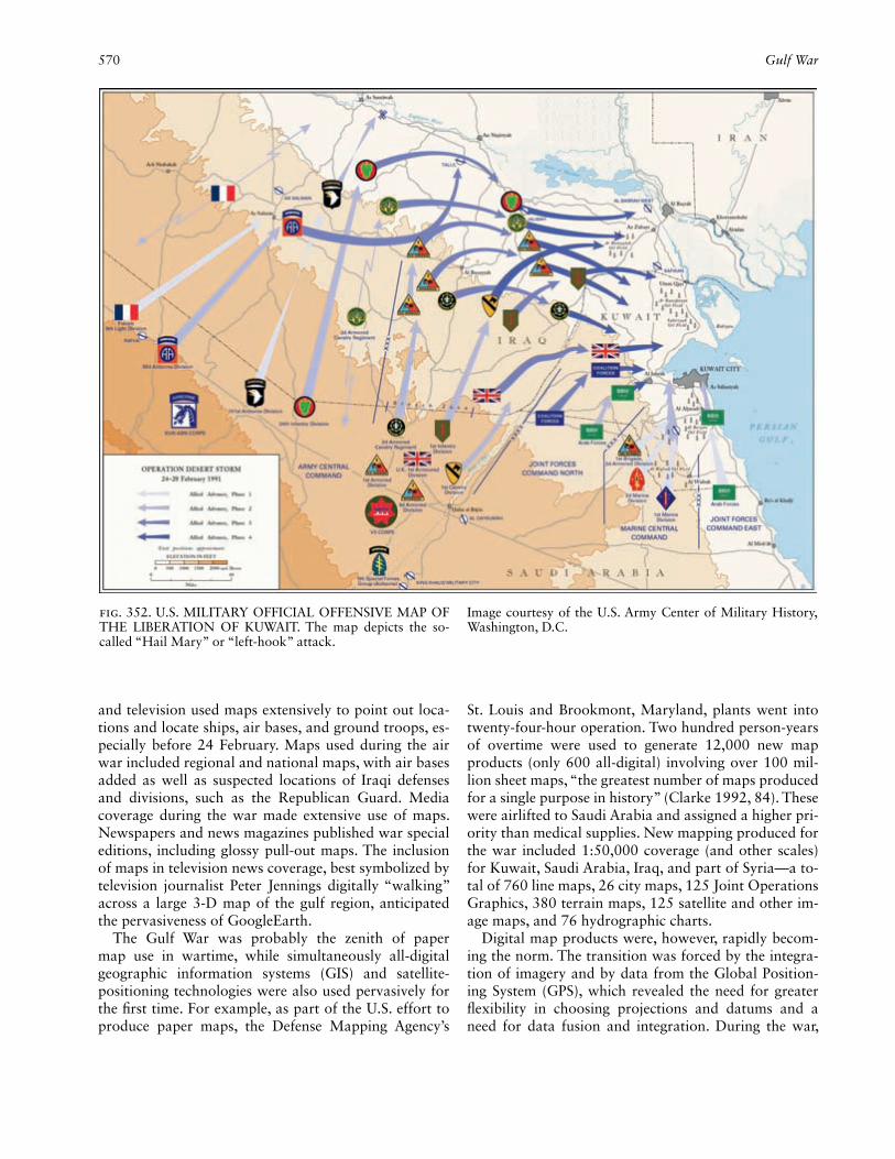
570 Gulf War

and television used maps extensively to point out loca-tions and locate ships, air bases, and ground troops, es-pecially before 24 February. Maps used during the air war included regional and national maps, with air bases added as well as suspected locations of Iraqi defenses and divisions, such as the Republican Guard. Media coverage during the war made extensive use of maps. Newspapers and news magazines published war special editions, including glossy pull-out maps. The inclusion of maps in television news coverage, best symbolized by television journalist Peter Jennings digitally “walking” across a large 3-D map of the gulf region, anticipated the pervasiveness of GoogleEarth.

The Gulf War was probably the zenith of paper map use in wartime, while simultaneously all-digital geographic information systems (GIS) and satellite-positioning technologies were also used pervasively for the fi rst time. For example, as part of the U.S. effort to produce paper maps, the Defense Mapping Agency’s

St. Louis and Brookmont, Maryland, plants went into twenty-four-hour operation. Two hundred person-years of overtime were used to generate 12,000 new map products (only 600 all-digital) involving over 100 mil-lion sheet maps, “the greatest number of maps produced for a single purpose in history” (Clarke 1992, 84). These were airlifted to Saudi Arabia and assigned a higher pri-ority than medical supplies. New mapping produced for the war included 1:50,000 coverage (and other scales) for Kuwait, Saudi Arabia, Iraq, and part of Syria—a to-tal of 760 line maps, 26 city maps, 125 Joint Operations Graphics, 380 terrain maps, 125 satellite and other im-age maps, and 76 hydrographic charts.

Digital map products were, however, rapidly becom-ing the norm. The transition was forced by the integra-tion of imagery and by data from the Global Position-ing System (GPS), which revealed the need for greater fl exibility in choosing projections and datums and a need for data fusion and integration. During the war,

Fig. 352. U.S. MILITARY OFFICIAL OFFENSIVE MAP OF THE LIBERATION OF KUWAIT. The map depicts the so-called “Hail Mary” or “left-hook” attack.

Image courtesy of the U.S. Army Center of Military History, Washington, D.C.

Fig. 353. A DEFENSE MAPPING AGENCY JOINT OPERA-TIONS GRAPHICS (JOG) SAVED FROM AN AIRCRAFT COCKPIT DURING THE AIR WAR.

Size of original: 46.5 × 41.8 cm. Private Collection. Im-age courtesy of Adam Campbell, Gumball Productions, San Diego.

572 Gulf War

the Selective Availability (SA) option on the GPS was turned off, and numerous operational problems with the satellite constellation were solved, partly by expediting the launch of several GPS satellites. Imagery added to the mapping process included intelligence sources from overhead satellites, and the JointSTARS imaging radar system that could image in poor weather and at night (Clarke 1992, 85–86).

The impact of the Gulf War on cartography as a whole produced a recognition of the power of advanced high-technology systems and the realization that mapping intelligence (now termed GEOINT—geospatial intelli-gence) contributed directly to the success of the Allied war efforts. This continued to be true during the war’s aftermath, when priorities shifted to the relief effort, en-forcement of continuing sanctions, and remediation of

environmental contamination caused by depleted ura-nium, oil fi res on land, and deliberate oil leaks at sea.

Keith C. Clarke

See also: Cruise Missile; Journalistic Cartography; Military Mapping of Geographic Areas: Middle East; Warfare and Cartography

Bibliography:Anonymous. 1991. “GIS Used in Operation Desert Storm.” ACSM

Bulletin 131:15.Clarke, Keith C. 1992. “Maps and Mapping Technologies of the Per-

sian Gulf War.” Cartography and Geographic Information Systems 19:80–87.

Finlan, Alastair. 2003. The Gulf War 1991. Oxford: Osprey.Kwarteng, Andy, and Pat S. Chavez. 1998. “Change Detection Study

of Kuwait City and Environs Using Multi-temporal Landsat The-matic Mapper Data.” International Journal of Remote Sensing 19:1651–62.

Zelizer, Barbie. 1992. “CNN, the Gulf War, and Journalistic Practice.” Journal of Communication 42:66–81.