Policy Research Working Paper 7422

The Heterogeneous Effect of Information on Student Performance

Evidence from a Randomized Control Trial in Mexico

Ciro Avitabile Rafael de Hoyos

Education Global Practice GroupSeptember 2015

WPS7422P

ublic

Dis

clos

ure

Aut

horiz

edP

ublic

Dis

clos

ure

Aut

horiz

edP

ublic

Dis

clos

ure

Aut

horiz

edP

ublic

Dis

clos

ure

Aut

horiz

ed

Produced by the Research Support Team

Abstract

The Policy Research Working Paper Series disseminates the findings of work in progress to encourage the exchange of ideas about development issues. An objective of the series is to get the findings out quickly, even if the presentations are less than fully polished. The papers carry the names of the authors and should be cited accordingly. The findings, interpretations, and conclusions expressed in this paper are entirely those of the authors. They do not necessarily represent the views of the International Bank for Reconstruction and Development/World Bank and its affiliated organizations, or those of the Executive Directors of the World Bank or the governments they represent.

Policy Research Working Paper 7422

This paper is a product of the Education Global Practice Group. It is part of a larger effort by the World Bank to provide open access to its research and make a contribution to development policy discussions around the world. Policy Research Working Papers are also posted on the Web at http://econ.worldbank.org. The authors may be contacted at cavitabile@worldbank.org.

A randomized control trial was conducted to study whether providing 10th grade students with information about the returns to upper secondary and tertiary education, and a source of financial aid for tertiary education, can con-tribute to improve student performance. The study finds that the intervention had no effects on the probability of taking a 12th grade national standardized exam three years after, a proxy for on-time high school completion, but

a positive and significant impact on learning outcomes and self-reported measures of effort. The effects are larger for girls and students from households with a relatively high income. These findings are consistent with a simple model where time discount determines the increase in effort and only students with adequate initial conditions are able to translate increased effort into better outcomes.

The Heterogeneous Effect of Information on Student Performance: Evidence from a Randomized Control Trial in

Mexico

Ciro Avitabile and Rafael de Hoyos

Keywords: information, returns to education, school performance, RCT

JEL No. I25, D80, O12

The Heterogeneous Effect of Information on StudentPerformance: Evidence from a Randomized Control

Trial in Mexico∗

Ciro Avitabile† Rafael de Hoyos‡

September 2015

1 Introduction

Early work for developing countries finds that providing information about the labor marketreturns to education had a positive impact on student attainments (Jensen 2010; Nguyen2008).1 These results, coupled with the low costs of these interventions, have induced schol-ars and policy makers to advocate for a more extensive usage of information interventionsto boost students’ outcomes in developing countries.2 However, while there is growing con-∗The paper has been screened to ensure no confidential information is r evealed. The original design of the

Percepciones project benefited f rom d iscussions w ith Erik B loom, Robert J ensen and Harry P atrinos. We are especially indebted to Martha Hernández, Elizabeth Monroy and Paula Villaseñor who were responsible for project and data management at the Mexican Secretariat of Public Education (SEP) at the time of implementing the project. We thank Caio Piza, Laura Trucco and participants at the World Bank’s impact evaluation seminar (DIME) and Banco de México for their comments. The authors gratefully acknowledge funding from the World Bank’s Research Support Budget.†The World Bank. 1818 H Street NW, 20433 Washington DC. Corresponding Author. E-mail: cav-

itabile@worldbank.org.‡The World Bank. 1818 H Street NW, 20433 Washington DC. E-mail: rdehoyos@worldbank.org.

1Jensen (2010) finds that providing information about the returns to lower secondary has a very large impact on school completion rates among eight graders in the Dominican Republic. Nguyen (2008) shows an increase in attendance of fourth graders in Madagascar as a result of information about the labor market returns to lower secondary education. More recently, Dinkelman and Martínez (2014) find that information about financial aid for tertiary education had a significant impact on college preparatory enrollment, school attendance, and financial aid knowledge among eight graders in Chile. Loyalka et al. (2013) finds that providing information on college costs and financial aid to high school students in poor regions of northwest China increases the probability of attending college.

2A number of studies analyze the impact of information about the benefits and costs of higher education on students’ perceptions in developed countries (see, among others, Oreopoulos and Dunn (2013) for Canada and McGuigan et al. (2012) for the UK.)

sensus that quality - rather than quantity - of education is an important driver of economicgrowth (Hanushek and Woessmann 2008; Hanushek and Woessmann 2012), it is unclearwhether information interventions can have long-lasting impact on student achievements. Ifstudents expect labor market returns lower than the observed ones, information interventionsmight be able to increase their effort, and ultimately improve their performance in school.Existing evidence shows either short term positive impact (Nguyen (2008) for Madagascar)or no impact (Fryer (2013) for the US) on learning in early grades.3 This paper presentsevidence from a randomized control trial conducted in Mexico to study whether an informa-tion intervention targeting 10th grade students had an impact on their performance in 12thgrade.4

Mexico, as well as other middle-income countries, has reached almost universal enrollmentrates in primary and lower secondary, but still faces important challenges in the educationsystem, especially in upper secondary. Only six out of every ten students who enroll inupper secondary education graduate. Education achievements are characterized by largedisparities, with those accounted for by gender being particularly striking. Although girlsperform at least as well as boys throughout primary and lower secondary education in allsubjects, as witnessed by their scores in 6th and 9th grade national census based standardizedtest - Evaluación Nacional de Logro Académico en Centros Escolares (ENLACE), girls falldramatically behind boys in 12th grade math scores (see Table 1). While the quality of schoolsupply might play an important role, there is not full clarity on the individual characteristicsthat can explain the attainment and the achievement gaps. Financial constraints, lack ofinformation and social norms may be important demand side factors behind the high dropout and low learning outcomes, but disentangling their role is empirically challenging.

In 2009 the Mexican Secretariat of Public Education (SEP for its acronym in Spanish),in an attempt to improve on-time graduation and learning outcomes in upper secondary,designed and implemented an intervention to provide students entering 10th grade with arange of information about the returns to upper secondary and tertiary education, as wellas on life expectancy and funding opportunities for tertiary education. The pilot program,known as Percepciones, included an evaluation strategy based on a stratified randomizedcontrol trial (RCT), with 26 schools assigned to the treatment group and 28 to the controlgroup. In November 2009 the baseline data was collected and the information treatment wasdelivered. Using 2012 administrative data from the 12th grade national standardized EN-

3Nguyen (2008) shows an increase in test scores of fourth graders in Madagascar three months after theintervention. Fryer (2013) finds no impact on student scores in sixth and seventh grade.

4Throughout the paper we will use upper secondary education and high school indifferently when we referto grades 10 to 12. We will use lower secondary when referring to grades 7 to 9.

2

LACE exam, we measure the impact of the information treatment on a proxy for completingupper secondary on time and standardized test scores in math and language (Spanish). Weshed light on some of the behavioral responses induced by the intervention using informationfrom a survey that was administered at the time of the test to a random sample of examtakers.

Our results show that, almost three years after the treatment was implemented the in-formation package had no impact on the proxy for completing high school on time. Onaverage, the intervention had a large and statistically significant impact on math test scores(0.29 standard deviations), and a positive but not statistically significant impact on languagescores. A more detailed analysis shows that the treatment had a large and significant effecton the learning outcomes of female students and those who belong to relatively better offhouseholds. Both boys and girls update their expectations as a result of the intervention,but only girls report a higher level of effort and switch to more demanding upper secondarysubtracks, with higher expected returns in the labor market. Neither the initial level of infor-mation about returns to education nor differences in time preferences seem to explain muchof the differential effect for boys and girls. There is also no evidence that the gender relatedheterogeneity is driven by gender-specific parents’ or teachers’ responses. We conjecturethat at least in the sample we consider, boys have lower scope to increase their effort. Thestronger impact on better-off students is consistent with the hypothesis that the increase ineffort can translate into better learning outcomes only if complemented with sufficient initialconditions as proxied by household income.

The contribution of this paper is twofold. First we contribute to a better understandingof the effects of information on different educational outcomes. The very large and significanteffects on school attainments in rural Dominican Republic (Jensen 2010) and Madagascar(Nguyen 2008) contrast with the zero impact found for the US (Fryer 2013), China (Loy-alka et al. 2013) and Mexico in this paper. In low income countries, providing informationabout school returns might be sufficient to induce at-risk students to stay in school sincethe alternative option may be particularly low. However, in medium and high income coun-tries, the higher probability of finding a paid job might induce at-risk students to drop out,irrespective of how well informed they are.5 Unlike previous work, we provide evidence onthe impact of information on learning at the end of high school, an outcome that is likely tobe correlated with youth labor market outcomes (Murphy and Peltzman 2004). The aver-

5Atkin (2012) finds for Mexico that the employment opportunities for low-skill workers in the manufac-turing sector generated by trade liberalization had significant consequences on school drop-out: for everytwenty new jobs created in the manufacturing sector, one student dropped out at grade nine rather thancontinuing on through grade twelve.

3

age impact is non-negligible and statistically significant, and given the virtually zero cost ofthe intervention this result provides further support to the cost-effectiveness of informationinterventions.

In many disadvantaged contexts educational choices made by girls are likely to be affectedby social norms, rather than potential labor market outcomes.6 Information interventionsas the one included in the Percepciones program can be an effective way of changing girls’educational choices, improve their learning outcomes and, eventually their labor marketoutcomes.

The paper is organized as follows. Section 2 presents general information regarding theupper secondary education system in Mexico and a description of the information treatmentwithin the Percepciones project. In Section 3 we discuss a simple framework to describe howinformation can affect student performance together with the data used for our analysis. Theeconometric model and the main results are presented in Section 4. Potential explanationsfor the large gender heterogeneity are discussed in Section . Finally, Section 6 concludes andprovides policy recommendations.

2 Context

The upper secondary education (EMS for its acronym in Spanish) system in Mexico consistsof 4.1 million students, typically between 15 to 18 years old, in grades 10th, 11th and 12th.EMS is offered by four different providers: 1) the federal government (accounting for 26% oftotal enrollment), 2) the state government (43.8%), 3) publicly-financed autonomous univer-sities (12.5%), and 4) private entities. EMS offers three types of degree programs: general –preparing students for higher education, technological – preparing students both for the labormarket as well as for higher education, and technical – emphasizing technical and vocationaleducation. The typically large technological schools run by the Federal Government (930students on average) can belong to different subsystems according to their specialization:industrial (DGETI), agricultural (DGETA) and ocean-related (DGCYTM).

According to the official statistics from SEP,7 in 2013 only 61% of students graduatedthree years after enrolling, with this share being significantly higher among women (65%)than men (57%). Graduation rates vary across types of degree programs with general schools

6Attanasio and Kaufmann (2012a) found for Mexico that educational choices of boys are more likely tobe correlated with expectations on the labor market returns of higher education than girls’ expectations,which display a stronger correlation with their aspirations to form a family. Kaufmann et al. (2013) usedata from Chile to show that being admitted to a higher ranked university has substantial returns in termsof partner quality for women.

7See http://www.inee.edu.mx/index.php/bases-de-datos/banco-de-indicadores-educativos

4

showing the highest (64%), followed by technological schools with rates very close to thenational average and technical schools showing the lowest (48%). More than 60% of thecumulative dropouts throughout the three years of EMS take place during the first year.The decision behind early drop out can be partly explained by the combination of highrisk of repetition (the average grade repetition rate was about 15% in 2013) and the strictpromotion criteria used in EMS. Students must pass five out of eight disciplinary subjectareas and practical modules, otherwise they have to repeat the semester. Additionally,students must pass all their subject areas and modules (around eight in total per semester)within ten semesters after enrolling in EMS, otherwise they lose the right to re-enroll.

The Percepciones pilot took place in 54 technological EMS schools run by the FederalGovernment. The objective of the Percepciones pilot was to evaluate the effectiveness of alow cost information intervention to increase on-time high school graduation and increaselearning outcomes. The design of the Percepciones project benefited substantially fromthe survey collected in 2005 as part of the evaluation of the Mexican program Jóvenes conOportunidades. The 2005 survey showed that there was a misperception about the returns toeducation when compared to the returns from the labor survey ENOE (Encuesta Nacionalde Ocupación y Empleo), especially among girls, thus providing scope for the intervention.8

A randomized control trial was designed to evaluate the impact of the intervention. Figure1 shows the time line of the project spanning from May 2009 to May 2012. The design ofthe intervention, randomization and sampling took place between June and August 2009.Following a two-step stratified sampling by regions (north, center, and south), the 54 schoolswere randomly allocated into 26 treatment schools and 28 control schools. The selectedschools had an average of 8 classrooms in 10th grade, with around 40 students in eachclassroom. For each school, at least two 10th grade classrooms were randomly selected toparticipate in the pilot. In total, 111 classrooms and 4,145 students were included in theexperiment.9

2.1 Description of the Treatment

The intervention was conducted in November 2009 (Figure 1). An interactive computersoftware, designed explicitly for the project, gathered information on students’ perceivedreturns to schooling and, in the case of the treatment group, provided the informationpackage. Given the design of the intervention, all of the students in the treatment group

8See Attanasio and Kaufmann (2012b) for a detailed description of the expectations module included inthe Jóvenes con Oportunidades survey.

9For two schools the first two randomly selected classrooms were too small, and additional classroomshad to be selected.

5

who completed the baseline survey were exposed to the information, thus guaranteeing perfectcompliance.

In order to elicit the information on perceived returns to schooling, the computer softwareused three subjective expectation questions, similar to the ones included in the Jóvenes conOportunidades survey:

1. If you were to quit studying right now and hence lower secondary is your highest degree,what do you think is the amount you can earn per month at ages 30 to 40?

2. If you finish upper secondary and do not continue studying, what do you think is theamount you can earn per month at ages 30 to 40?

3. If you get a university degree and do not continue studying, what do you think is theamount you can earn per month at ages 30 to 40?

Similarly, the computer software elicited information about the students’ perceptionabout the returns to schooling for an average person, as opposed to expectations abouthis or her own returns.10 Students in the treatment group received three main informationcontents. First, they were given gender-specific information on the monetary returns toschooling, as computed using data from ENOE second quarter of 2009. The information onthe returns to education was given in the form of additional monthly pesos earned by uppersecondary working full time as well as the net present value of the additional income flowsassuming entry and exit to the labor market at ages 25 and 65, respectively:

In Mexico a man (woman) between 30 and 40 years old with a maximum educa-tion level of lower secondary earns, on average, $4,832 ($3,179) MX per month.11

A man (woman), ages 30 to 40, with an upper secondary diploma earns, on av-erage, $6,466 ($4,827) MX per month, or $1,634 ($1,648) MX more per month.Therefore a man (woman) with an upper secondary diploma earns, on average,$784,320 ($791,040) MX more than those with a lower secondary degree through-out his (her) productive life.

Students in the treatment group also received information about the returns to univer-sity in a format similar to the one presented above. The second type of information content

10The three questions read as follows: (1) what do you think is the amount earned per month by a man(woman) between 30 and 40 years old with a lower secondary degree?; (2) what do you think is the amountearned per month by a man (woman) between 30 and 40 years old with an upper secondary degree?; (3)what do you think is the amount earned per month by a man (woman) between 30 and 40 years old with auniversity degree?

11In November 2009 $1 MX was approximately $0.08 US.

6

is about a higher education scholarship program run by the federal government (PRON-ABES). While most of the Mexican higher education system is public and free of charge,the PRONABES program targets student from households with a monthly income equal toor below three minimum wages, and provides grants that vary from $750 MX to $1,000 MXper month for the entire length of the higher education course. Finally, students receivedinformation about life expectancy (differentiated by gender). Additionally, a 15-second videosummarizing the message that youth can empower themselves with education was shown tothe students in the treatment group.

Most of the interventions that have been previously tested provide information either onthe expected financial returns of education (Jensen 2010; Nguyen 2008) or on the sources offinancial aid (Dinkelman and Martínez 2014).12 The Percepciones project gave students aninformation package, that covers the financial returns of secondary and tertiary education,one source of financial aid for tertiary education and life expectancy. The intervention’sdesign does not allow for the assessment of whether our results are driven by any specificpiece of information or by the entire package.

3 Conceptual Framework and Data

3.1 Conceptual Framework

We borrow the simple two period framework presented in Fryer (2013) to help rationalize thelinkages between the information intervention and student outcomes. Student’s educationoutcomes (S) at time t is a function (f) of her/his effort (e) and a set of predeterminedcharacteristics (µ0), that include, among others, parental education, household income, andneighborhood characteristics.

Si,t = f(ei,t, µ0i) (1)

Mirroring Fryer (2013), we assume that: a) f is twice continuously differentiable in e

and µ0; b) f exhibits diminishing marginal returns to e; c) e and µ0 are complements in theeducation production function. At time t+1 the student enters the labor market and his/herlabor market outcomes (Y ) are a function of the school outcomes at time t and a parameter(ν), that measures students’ perceived returns to education outcomes. Both attainmentsand performance in school are likely to affect Y . We assume that earnings are increasing in

12An exception is McGuigan et al. (2012) that tests the impact of a large set of information about thebenefits and costs of university on the perceptions of high school students in the UK.

7

S, although at a declining rate. Increases in the perceived returns, ν, increase Y at all levelsof S.

maxe [β [Yi,t+1(Si,t(ei,t), ν)]− C(ei,t)] (2)

The individual chooses effort at time t maximizing the future earnings discounted at thetime discount rate β, minus the cost of effort (C(e)). In this very simple setting, informationabout returns to education will increase the optimal level of effort to the extent that: a) thestudent’s perceived returns are significantly lower than the actual returns; and b) the studentplaces a significant value to future consumption (high β). However, an increase in effort doesnot necessarily generate an increase in student performance. In fact, if the complementaritybetween e and µ0 does not hold and/or the student does not know how to translate increasedeffort into better outcomes, an increase in effort might not lead to improved performance.

3.2 Baseline Data

In order to measure students’ characteristics at the baseline, we use two sources. First, werely on the survey administered to the students in November 2009, just before the treatmentwas rolled out. In addition to providing information about the perceived returns to schooling,students were asked, among others, questions about the source of information about thereturns, household income,13 parents’ education and work status. The baseline survey alsoincluded a module that elicits students’ inter-temporal preferences. The respondent wasasked to consider a hypothetical situation in which he/she wins a certain amount of moneythat can be cashed in now, or can be cashed in later for a larger sum.

Second, we use administrative data on 9th grade ENLACE scores in math and languageto measure students’ ability before entering high school. From 2007 to 2013, ENLACE wasadministered to all students in 3rd to 9th and 12th grades. The test is voluntary and bearsno consequences either on graduation or a student’s GPA. The score is normalized to havea mean of 500 and a standard deviation of 100. Mexican citizens have a unique personalidentifier, known as Clave Única de Registro Poblacional, CURP, formed by an algorithmcombining name, surname, date of birth, sex, state of birth, plus 2 randomly generateddigits. Using the student’s personal information collected during the baseline survey wecould generate a quasi-CURP that only differs from the original one for the lack of the last

13Information regarding household income was reported in brackets as follows: 1) less than $1,500 MX, 2)between $1,501 and $3500, 3) between $3,501 and $7,000, 4) between $7,001 y $10,000, 5) between $10,001and $15,000, 6) $15,001 y $25,000, 7) more than $25,000 MX. Information about household income was notreported by 14% of the students, but the attrition rate is not statistically different for the treatment andcontrol group.

8

two randomly generated digits making possible a merge between the baseline survey withthe micro data from ENLACE 9th grade.14 For 75.5% of the students in our sample, wecan recover their 9th scores ENLACE score, with 68% taking the exam in 2009, 1.1% in2007 and 0.4% in 2006.15 There are two potential explanations for the partial attrition of9th grade scores: 1) the exam is voluntary and students enrolled in upper secondary mighthave not taken it; 2) matching related issues either because the information provided duringthe baseline was not sufficient to generate the quasi-CURP, or for the presence of multipleindividuals with the same identifier. Only for five individuals out of 4,145 we were not ableto generate a quasi-CURP.

Table 2 shows the baseline characteristics, for the full sample as well as separately forboys and girls, distinguishing between students in the treatment and the control groups.In the top panel we report the socioeconomic characteristics measured through the baselinesurvey, in the bottom panel the administrative information on 9th grade test scores. Overall,the characteristics of the treatment and control group seem well balanced in line with therandomized design of the evaluation. For boys we find that, out of 23 variables, only theprobability that the father works is statistically higher in the treatment than in the controlgroup (p-value=0.011), but the size of the difference is economically negligible. In orderto account for these imbalances, our main specification controls for all the variables thatdisplay significant imbalances. On average, 93% of the fathers work, as opposed to 45% ofthe mothers; fathers tend to be more educated than mothers, since 31% of the formers have,at least, completed high school as opposed to 24% of the latter. About 40% of the studentshave access to an Internet connection at home.

Self-reported measures of effort do not display major differences between boys and girls,neither when we consider the number of hours spent doing homework (5.62 for boys and5.11 for girls), nor when we look at the number of school days missed last month (2.8 forboys and girls). Girls report a much lower probability of having failed at least one subjectin lower secondary school than boys (19% versus 30%).

Students in the treatment group are more likely to be matched with 9th grade test scoreresults and the difference is marginally significant at 10%. In 9th grade girls perform betterthan boys in language, irrespective of whether we consider the test score or the probabilityof being classified as insufficient, and they do as well as boys in math (approximately 35% ofthem are classified as insufficient). Previous work using data from low- and middle-income

14Given that the CURP and the information to form the quasi-CURP is confidential, the merge betweenthe baseline survey information and the micro information of ENLACE was done by staff at the SEP.

15Students who could be matched with 9th grade score are different from those who could not be matchedalong some dimensions (see Table AI) but most differences are economically small.

9

countries shows that the gender gap in math is present as early as 4th grade (Bharadwaj et al.2012). This is not the case for Mexico. In order to assess whether our sample is representativeof the Mexican population, we follow the nationwide cohort of 6th grade ENLACE takers inthe year 2007 over to 9th (in 2010) and 12th grade (in 2013). Girls do consistently betterthan boys in language and the gap stays constant throughout the different grades. Neitherin 6th grade nor in 9th grade is there evidence of a gender gap in math, but girls’ 12th gradescore in math is 30 points (0.30σ) lower than boys’ (Table 1). The gender gap in 12th grademay be partly explained by differential selection: 28.6% of the boys who took the ENLACE6th grade in 2007 completed the 12 grade exam in 2013, as opposed to 34.9% of the girls.

3.3 Follow-up Data

Students enrolled in 10th grade in 2009 were supposed to complete high school in 2012.16 Weuse data from the 2012 12th grade ENLACE exam to measure the three main outcomes ofinterest: the probability of taking the test, math scores, and Spanish scores. We interpret theprobability of taking the 12th grade test in 2012 as a proxy for the probability of completingupper secondary on time. 61% of the students surveyed at the baseline took part in the12th grade ENLACE exam three years later. Not observing a student who was originallyenrolled in EMS in 2009 take part in the 12th grade ENLACE exam in 2012 has four possibleexplanations: 1) the student dropped out of school at any point between 9th and 12th grade,2) the student repeated one or more semesters, 3) the student did not show up for the exambut regularly completed the EMS, 4) or potential merging problems. Using 2013 data from12th grade ENLACE we find that 205 students from the original sample (4.9%) took theexam in 2013, most likely because they had to repeat two full semesters.17 The probabilityof taking ENLACE in 2013 is not statistically different for treatment and control schools. Inorder to provide a measure of the no-showing up rate, we collected the 2012 lists of all thepotential 12th grade ENLACE takers that each school had to send to the central authorityroughly two months before the test. On average, 10% of the students reported on the list didnot show up for the exam, but they are likely to complete EMS regularly. Reassuringly, theno-showing-up rate is not statistically different for treatment and control schools. Finally,only for five students the quasi-CURP was not sufficient to identify them since it was notunique. Therefore, we interpret the difference in probability of taking the 12th grade exambetween the treatment and control groups as a good measure of the intervention’s effect on

16The northern State of Nuevo León is an exception since public upper secondary schools follow a two-yearprogram.

17Students who repeat either one or three semesters leave school without taking the test.

10

the probability of finishing upper secondary on time.In order to measure how expectations about the returns to education have changed in

response to the intervention, we rely on the data from a nationwide survey administeredto 20% of all 12th grade exam takers, the so called ENLACE de contexto. In our sample,730 students were administered the ENLACE de contexto. The 2012 survey gathers, amongothers, information on expected monthly earnings at ages 30 to 40 on two hypotheticalscenarios of educational attainments, high school completion and university degree. Thesequestions read exactly the same as the ones asked in the baseline survey, but the answersare given using a pre-codified set of brackets.18

The ENLACE de contexto does not collect objective measures of student effort but itelicits self-reported assessment. The respondent is asked how the statement “I am a personwho works hard in school” describes him or her in one of the following ways: 1) it does notdescribe me at all, 2) it describes me a little bit, 3) it describes me, 4) it describes me a lot,5) it fully describes me. Students are also asked which subtrack they chose as part of thetechnological school curriculum.

3.4 Perceptions about Returns to Schooling

As discussed in section 2.1, the baseline survey asked both about student’s own expectedearnings and the student’s expected returns for the average person. While variation inthe perceived returns for oneself reflects both possible misperceptions about the educationreturns and heterogeneity in subjective valuations of how well oneself can do in the labormarket, dispersion in perceived average returns would just reflect misperception. Table 3reports the gender specific mean and standard deviation of the expected monthly wages forthemselves and for the average person, separately for the treatment and the control group.For none of the measures of perceived returns, the difference between the treatment and thecontrol group is statistically significant.19

At the baseline, the mean expected monthly wage for oneself, having completed highschool as the highest degree, among boys in the control schools ($5,531 MX) is not staticallydifferent from the average wage for a man with high school degree between 30 and 40 usingdata from ENOE ($5,722 MX). When asked about the expected wage for an average manbetween 30 and 40, the average expected value is substantially lower ($4,282 MX). On

18The earnings brackets for both questions are: i) $4,000 MX or less; ii) $4,001 MX to $7,000 MX; iii)$7,001 MX to $10,000 MX; iv) $10,001 MX to $15,000 MX; v) $15,001 MX to $20,000 MX; and vi) morethan $20,000 MX.

19The statistics displayed in Table 3 are generated trimming the top 1% and the bottom 1% of the earningsexpectations, but the balancing properties still hold in the untrimmed sample.

11

average, a girl in the control group expects to earn $4,101 MX, as opposed to an averageestimated wage of $4,827 MX for a woman with high school degree between 30 and 40 yearsold, according to ENOE. The average expected wage for the average woman is $3,154 MX.

Comparing the mean expected wages with observed values might not be particularlymeaningful in the presence of highly skewed expected income distributions. In order to betterunderstand the extent of the misperceptions, we discretize the baseline answer applyingthe thresholds used in the follow-up data source - i.e. 12th grade ENLACE de Contexto.Figures 2 plots the distribution of expected wages (self) at the baseline against the observeddistribution in the 2009 ENOE separately for boys and girls. The largest difference betweenperceived and observed earnings realizations are concentrated in the first two bins of thedistribution; the fraction of both boys and girls who think that they will earn less than$4,000 MX is much larger than the actual fraction of high school graduates earning 4,000or less in the second trimester of 2009. For earnings higher than $7,000 MX we do notobserve significant differences between the distribution of the expected earnings (self) andthe current ones. The extent of this misperception becomes even more evident when weconsider the distribution of the expected earnings of an average person between 30 and 40and compare it with ENOE (Fig. AI).

Both for boys and girls the income expectations upon completing university are on averagehigher than the wages observed for a university graduate between 30 and 40 years old, asmeasured in the ENOE data. This is true irrespective of whether or not we consider theincome expectation for oneself or for the average person.

In summary, the average perception on the wages that each of them can earn upon com-pleting upper secondary is aligned with the average wage observed in the labor market.However, there is a large fraction of boys and girls who tend to underestimate the earningsof a high school graduate in the labor market. According the to the baseline survey, 79% ofthe respondents mentioned family members as one of the three main sources of informationabout the benefits of studying, followed by television (70%) and internet (48%). In order toprovide prima facie evidence on the link between expected earnings and school performance,Table 4 shows the correlation between baseline expectations about future earnings, expressedin logarithms, and follow-up outcomes for the individuals in control schools. The correlationbetween the expected log earning upon completing either upper secondary or tertiary educa-tion and the probability of being identified in the 2012 ENLACE 12th grade is small and notstatistically significant, regardless of whether or not we consider the expectations for oneselfor the average person. We do find evidence of a significant correlation between the expectedearnings and the results in math and Spanish. The correlation is particularly strong and

12

statistically significant when we consider the expectations for oneself (columns 5-6 and 9-10in Table 4), rather than for the average person. Although the association does not haveany causal interpretation, it does suggest that expectations of students upon entering highschool, especially the ones for oneself, do bear some relation to final performance.

4 Empirical Analysis

4.1 Econometric Model

To estimate the causal impact of providing information about the labor market returns ofeducational attainments, we estimate the following equation:

Yij = β0 + β1Dj + γ′Xij + uij (3)

where Yij is the outcome of student i in school j recorded in the follow-up survey. Dj isan indicator dummy that takes the value one if school j is assigned to the treatment group,0 otherwise. β1 measures the average treatment on the treated (ATT) effect of receiving theinformation in the modalities explained above. Let Xij be a vector of baseline covariatesmeasured at the individual and school level. In our main specification, Xij includes themacro-regions where the school is located (north, center and south) - the level at whichthe randomization has been stratified, dummies for the type of specialization of the school(industrial, agricultural, or ocean-related), age and gender of the student, dummies for thelevel of proficiency in math and Spanish in the 9th grade ENLACE, and dummies for whetherthe 9th grade scores in math or Spanish are missing, dummies for whether the mother andthe father work, dummies for whether the information on father’s and mother’s work statusis missing, dummies to proxy for the presence PC and internet at home. In order to reducethe potential efficiency losses due to the multilevel design of our sampling - at least twoclassrooms were randomly selected both in treatment and control schools - we follow Cameronand Miller (2015) and in our main specifications we use a Feasible Generalized Least Square(FGLS) estimator. The results from the standard OLS, although slightly less precise, are inline with those presented and are available upon request. In all the specifications, standarderrors are clustered at school level to account for correlated shocks within schools, thatrepresent the level at which the treatment is assigned.

Both for math and Spanish, we standardize all the scores using the mean and the standarddeviation observed in the control group. In order to address the inference issues related tothe presence of multiple learning outcomes (Kling et al. 2007), we also consider the effect

13

on the average test score, as defined by the average of the standardized scores in math andSpanish.

When we study how the treatment effect varies along individual and household charac-teristics, the results are based on fully interacted models.

4.2 Results on Education Outcomes

In this section we describe the results of our experiment on the four main education outcomes:the probability of taking the 12th grade ENLACE on time - i.e. three years after the startof upper secondary, standardized Spanish test score, standardized math test score and theaverage of the two. In Table 5 we present the ATT effects for the whole sample. In theodd columns we present the results for the specification that only controls for the stratadummies, in the even columns we show the results of our main specification with the full setof controls.

Receiving information about returns to education had a positive, but not statisticallysignificant effect (coeff. 0.025 and standard error 0.042) on the probability of taking theENLACE test in 2012, thus suggesting that the intervention did not affect on-time highschool completion. In principle, if information about school returns is increasing students’incentives, we might have expected a higher probability of completing high school on time.

We next consider the effect on students’ learning outcomes. The results are presentedin columns 3 to 8 in Table 5. The treatment effect is equal to 0.16σ and not statisticallysignificant for Spanish and 0.32σ and marginally significant for math when we only controlfor the strata dummies. For the average of the two scores, we find an effect of 0.24σ,statistically significant at 10% level. When we include the full set of controls, the effect ofthe information treatment is equal to 0.10σ (not statistically significant) for Spanish, 0.29σfor math (significant at 5%) and 0.20σ (significant at 10%) for the average score. Since wefound no impact of the intervention on the probability of taking the ENLACE exam, it isunlikely that the effect on test scores are driven by differential selection into the ENLACEexam in treatment and control schools.

We next consider how the treatment effect varies with three important dimensions: gen-der, ability and household income. The experiment was not designed to be representativeat any of this level. Therefore our results have to be interpreted as suggestive, rather thanconclusive.

The intervention provided both boys and girls with gender specific measures of the returnsto human capital investment and its potential time horizon.20 We study whether boys and

20Increased life expectancy should increase the incentive to invest in schooling since a longer time horizon

14

girls responded differentially to the information provision. Results are presented in PanelA in Table 6. In the control group, girls are more likely to take the test than boys (63%vs 57%). Nevertheless, the effect of the information treatment on the probability of takingENLACE 12th grade on time is basically null for both boys and girls. In the control group,12th grade girls’ scores in language are better then boys’ but their scores in math are about0.40σ lower than for boys. This is somehow striking since the 9th grade score in math ofthe girls in the control group was 533 points as opposed to the 525 points for boys (seebottom panel in Table 2).21 When we look at the impact of the information treatmenton learning outcomes, for boys we find no effect on Spanish test scores, and a moderateand marginally significant increase in math scores (0.24σ). For girls we find a moderatepositive effect on scores in Spanish (0.17σ marginally significant at 10% level) and a large(0.34σ) and statistically significant impact on math scores. These impacts translate intoa 0.26σ (statistically significant at 5% level) increase in the average score for girls, and0.15σ statistically not significant increase for boys. We can reject the null hypothesis of nogender-differentiated effect on the average learning score (p-value=0.043)

According to SEP, students are classified in one of the following proficiency levels: a)insufficient, b) regular, c) good, and d) excellent, based on their ENLACE result. About16% and 30% of the students in our sample taking 9th grade ENLACE were classified asinsufficient in Spanish and math respectively. The 9th grade ENLACE proficiency level is astrong predictor of dropping out of upper secondary. In the control group, 40% of studentswith an insufficient 9th grade ENLACE math were not identified in 12th grade ENLACE,as opposed to 23% among those with a level of regular or more. We study the effect ofthe information for three different groups: a) those with an insufficient 9th grade ENLACE(henceforth low-ability students) in math, b) those with an ENLACE math score regularor better (henceforth high-ability students), c) those with a missing 9th grade ENLACEscore.22 Results are reported in Panel B in Table 6. The effect on the proxy for probabilityof finishing upper secondary on time is not statistically different from zero across the threesub-groups. When we look at learning outcomes, we find that among low-ability students,the effect is 0.04σ for Spanish and 0.25σ for math. For both subjects, the effect is notstatistically different from zero. For those with an ENLACE proficiency level of regular ormore, we find a large effect both on Spanish and math, 0.15σ and 0.33σ respectively, with

increases the value of investments that pay out over time.21As shown in Table 1, the gender differences in 9th grade scores observed in our sample are in line with

the nation wide difference reported in Table 1.22Table AII displays the balancing properties between treatment and control group in each of the three

subgroups. All the results reported in the paper are based on the student 9th grade classification in math,but they do not change when we use Spanish (results available upon request).

15

the average effect on test score being statistically significant. Nevertheless, when we comparewhether the program had a differential effect on the average learning score, we cannot rejectthat the effect for the low ability is the same as for high ability ones (p-value=0.18) andfor missing ability ones (p-value=0.31). In summary, although we find larger coefficients forhigh-ability students than low-ability ones, we do not have enough statical power to rule outthat the effect does not vary with initial level of ability.

We repeat a similar exercise using household income. We define as “high HH income”those students who report a monthly household income in the bracket between $3,501 MXand $7,000 MX or above, while those who report an income in a lower bracket are classifiedas “low HH income”.23 Results are reported in Panel C in Table 6. Household incomedoes not affect the program’s effect on the probability of taking the 12th grade ENLACEexam. The treatment effects on learning outcomes among low income students are notstatistically different from zero, although the size of the effect is nontrivial for the mathscore (0.20σ). Among high income students the effect is positive and marginally significanton Spanish (0.18σ) and large for math (0.32σ). When we consider the effect on the averagelearning score, we find a 0.12σ increase among low income students, as opposed to a 0.25σ(statistically significant at 5%) among high income students, and a 0.18σ increase amongmissing income students. We can reject the null hypothesis of no differential effect betweenlow and high income students (p-value=0.029), while we can not reject when we comparelow income students with those who do not report income information.

In summary, we found larger effects on the learning outcomes of girls than boys, mostlydriven by a particularly large impact on the math score. We found no significant evidenceof treatment heterogeneity in students’ ability, but significant differences associated withhousehold income. The fact that we found an effect only among high income studentsmakes unlikely that the average impacts that we find are driven by the infomation about thePRONABES higher education scholarship. As discussed in section 2.1, PRONABES onlytargets students with monthly household income below three minimum wages.

4.3 Results on Self-reported Effort

In the simple theoretical framework outlined in section 3.1, information improves student’sperformance through an increase in the level of effort. While objective measures of effort arenot available, we use the self-reported measure of effort elicited in the 12th grade ENLACEde contexto (described in section 3.3) to provide some preliminary evidence on whether theintervention induced students to work harder. 26% of the boys, as opposed to 18% of the

23In 2012, the median price adjusted household income was $4,880 MX.

16

girls, in the control group report that the statement “I am a person who works hard in school”describes them fully, while for 24% of the boys and 23% of the girls the statement describesthem a lot.

The major concern when using self-reported measures in a context like ours is the pos-sibility of social desirability bias: students in the treatment group might be more likely toreply in a way that will be viewed favorably by the others. The measure of self-reported ef-fort that we use was collected almost three years after the intervention as part of a standardnationally administered survey, and it is therefore unlikely that students could bias theirresponse as result of the information treatment. In general, self-reported data might capturepoorly the actual level of effort. In order to boost confidence in our measure, we use datafrom the control group to measure the correlation between the self-reported level of effortand the 2012 ENLACE results in math and Spanish. One standard deviation increase inself-reported effort leads to a 0.11σ increase in math and 0.12σ in Spanish. Both correlationsare statistically significant at conventional levels (results available upon request).

We use eq. 3 to study the impact of the information treatment on self-reported levels ofeffort. In order to simplify the interpretation of the results, we standardize the categoricalvariable using the mean and the standard deviation observed in the control group. Resultsare presented in Table 7. In column 1 we present the results for the entire sample. Overallthe treatment group reports a level of effort that is 0.24σ (statistically significant at 1%level) higher than for the control group. In column 2, we consider the effect by gender andwe find much larger impact for girls (0.35σ) than for boys (0.11σ). We can marginally rejectthe null hypothesis of no differential effect by gender (p-value=0.07). In column 3 we studyhow the effect on self-reported effort varies with the level of ability. We do find increases ineffort for all three subgroups discussed above (high- and low-ability students and those withno 9th grade ENLACE). The increase among low-ability students is larger in size (0.29σ)than among high-ability students (0.16σ). However, when testing whether the effect variesacross the three subgroups, we cannot reject the null hypothesis of no differential effect.In column 4 we show how the effect varies with household income. Both for low and highincome students we find large effects of the information package and also in this case we cannot reject the null hypothesis of no differential effect.

Although the self-reported nature of the data requires a cautious interpretation of theresults presented in this section, the information intervention seems to have improved stu-dents’ intrinsic motivation, irrespective of their ability level and their income level. The factthat learning outcomes only increase among high income students, although both high andlow income students report higher self-reported effort, is consistent with the hypothesis that

17

an increase in effort can translate into better learning outcomes only when complementedwith other inputs provided at home. An alternative explanation is that only students fromrelatively well-off backgrounds know how to translate increased effort into better outcomes.

We do find instead that boys and girls respond differentially to the intervention, with thelatter reporting higher levels of effort after receiving the information package. Therefore thegender-differentiated effect on learning outcomes documented in section 4.2 can be potentiallyexplained by the differential effect on effort.

5 Further Evidence on the Gender Heterogeneity

The results presented so far show that girls respond to the provision of information byincreasing their effort and, as a result, they display a large increase in test scores. Forboys, we find instead small and not statistically significant increases in self-reported effortand learning outcomes. In this section we further discuss the differential response of boysand girls, and provide some suggestive evidence on the possible mechanisms behind thesedifferences.

First, we study if both boys and girls update their beliefs in response to the informationtreatment. For this purpose, we rely on the information elicited as part of the 12th gradeENLACE de contexto. Two different types of caveats should be taken into account whencomparing the expected earnings collected at the baseline and at the follow-up. As alreadymentioned, the ENLACE de contexto only collects information among 20% of the entirepopulation of exam takers. Given the large share of students who dropped out before takingthe 12th grade ENLACE, the populations of exam takers and non-takers might differ alongboth observable and unobservable characteristics. This has the potential to introduce aselection bias. Due to the randomized assignment of the intervention, the selection biaswill not affect the internal validity of our results as long as it enters eq. 3 additively.Nevertheless, the external validity might be limited. Second, while the question regardingwage expectations included in the 12th grade ENLACE de contexto reads exactly as thequestion included in the baseline survey, the answer only allows the choice between the sixoptions described in section 3.4. In Fig. 3 we plot the distributions of expected earnings inthe treatment and the control group both for boys and girls in the follow-up. Compared tothe baseline, there is a higher proportion of boys and girls in the control group reportingan expected income in the bin where the observed average earnings fall. This might bethe result either of the selection into the exam taking, or improved information as studentsapproach the end of high school.

18

We observe a reduction in the probability of reporting an expected income (oneself)lower than $4,000 MX among boys and girls in the treatment group, compared to those in thecontrol group. Among girls in the treatment group, we observe an increase in the probabilityof reporting an expected income between $4,000 and $7,000 MX, and no changes in theprobability of reporting an expected income above $7,000. Among boys in the treatmentgroup, we instead observe no change in the probability of reporting an expected incomebetween $4,000 and $7,000 MX, but an increase in the probability of reporting an expectedincome in all the bins above $7,000 MX. The graphical evidence is supported by the regressionresults presented in Table 8. In summary, both boys and girls seem to update their beliefs inresponse to the information received as part of the intervention. However, while girls adjusttheir perceptions in line with the statistics provided, a significant fraction of boys reportvalues higher than information provided by ENOE.

It is puzzling that while both boys and girls update upwards their perceptions regard-ing the monetary benefits of finishing EMS, only girls report higher effort. We next assesswhether more objectives measures of effort support this conclusion. Until 2012, students at-tending technological EMS schools could choose among three different subtracks: 1) physicsand mathematics, 2) economics and accounting, and 3) chemistry and biology.24 Each sub-track has a large set of optional courses, and among those, students have to choose two (fora total of ten weekly hours) during the last semester of high school. The subtrack of physicsand mathematics is the one with the widest choice of math related courses, followed by theeconomics and accounting, and chemistry and biology.

We compare the school subtrack distribution for boys and girls in treatment and con-trol schools. Results are reported in Table 9. Among boys we do not find any significantdifference in the subtrack distribution between treatment and control groups; a vast major-ity of students prefer the physics and mathematics subtrack (48%) followed by economics(20%) and chemistry (13%). For girls, the percentage of students who prefer physics andmathematics is 27% and is not statistically different in the treatment and the control group.We do find instead a much larger fraction of girls undertaking economics in the treatmentgroups (35%) vis-a-vis the control one (19%), with a consequential reduction in the uptakeof chemistry and biology. A Kolmogorov Smirnov test allows us to reject the null hypoth-esis that the subtrack distribution is the same in the treatment and the control group forgirls, but we can not reject the null hypothesis for boys. This evidence shows that one ofthe mechanisms linking the information treatment with improved learning outcomes among

24Starting from 2012, as part of a major curriculum reform, students can have a fourth optional subtrack,that covers humanities and social sciences subjects (for details see http://cosdac.sems.gob.mx/riems.php).

19

girls took place via a change in their subtrack choices. One possible explanation for thisresult that the available data did not allow us to test, is that our intervention motivatedfemale students to search for more detailed information about the wages related to differentcareers and, as a result, opted for subtracks with higher expected returns but potentiallymore demanding. Since 2005 Mexico has a nationwide employment observatory (Observato-rio Laboral - OLA) that provides updated information on the main labor market outcomesof the different careers - including average wage and gender composition, and it can be easilyaccessed through a webpage.25

It is unclear why boys did not change their behavior, in spite of a more optimistic viewabout their returns to education. Following our simple conceptual framework, there aretwo potential explanations: 1) the distance between the perceived returns and the statisticprovided as part of the intervention differs for boys and girls; 2) boys and girls have differenttime preferences.

Only students with expected returns below the statistic provided as part of the interven-tion should increase effort and improve their results. At the baseline boys and girls do notstatistically differ in the probability of reporting an expected earning below the average earn-ing estimated with the ENOE (72% and 70% respectively), and therefore it is unlikely thatdifference in the baseline perceptions about future earnings can drive the gender differentialeffect of the information package on proxies for effort, and learning outcomes.

Lower time discount should lead to an increased impact of the program on effort. Thereis increasing evidence that men and women differ in time discount.26 In the baseline surveywe elicited information on time preference using a framework similar to the one used byRubalcava et al. (2009) and described in section 3.2. Consistent with their results, we findthat 20% of boys, as opposed to 15% of girls, would prefer accepting $3,000 MX today,regardless of the amount offered in one year time. We define these individuals as the "hightime discount" students, and "low time discount" as all students willing to give up the $3,000MX today in exchange for a larger sum in the future. We study whether the treatment effect

25According to the public information provided by the OLA in 2014, a nurse, one of the most commonprofessional outcomes for students choosing the chemistry and biology subtrack, receives on average $8,617MX per month and 87% of the nurses are female. The average wage for a clerk is $10,215 MX and $10,212 MXfor an accountant, two common outcomes for those opting for an economics and administration subtrack.Among clerks and accountants, women account for 49.3% and 46.4% of the total employees respectively.Careers such as engineering, that are common outcomes for those taking the physics and mathematicssubtrack, feature on average the highest wages but an extremely low proportion of women. The averagewages for a mining engineer and an automotive one are $19,838 MX and $14,036 MX per month respectively,but the percentage of women employed are 11.4% and 1.3%, respectively.

26See, among others, Dittrich and Leipold (2014) and Bauer et al. (2012). For Mexico, Rubalcava et al.(2009), using direct evidence on time preference from the Mexican Family Life Survey, finds that womenhave lower time discount than men.

20

varies with proxies for time discount. The evidence presented in column 1 in Table 10 showsthat low time discount students display a very large and significant increase in self-reportedeffort, as opposed to a zero impact among the high discount students. Point estimates onthe average learning score show larger coefficients for low time discount than high discountstudents (column 2 in Table 10), but we can not reject the null hypothesis of no differentialeffect.

In summary, both boys and girls update their priors about the labor market returns toeducation, but only the latter exert more effort, partly by choosing subtracks with highermathematical content. We provide some suggestive evidence that part of the difference mightbe explained by gender differences in time preferences. However, given the small difference inthe proportion of high discount students among boys and girls, and the fact that we can notreject the hypothesis that the effect on learning is the same for high and low time discountstudents, we conclude that the role of time preferences in explaining the gender-differentiatedeffect on learning is at most small.

There might be alternative explanations behind the gender-specific response to the in-formation treatment. Information about future returns to children’s education might inprinciple affect parental expectations and, as a result, their investments into their children’shuman capital. Parents might invest more in girls if they were underestimating their futurelabor market returns.27 Similarly, teachers in treatment schools might have increased theireffort, possibly as a result of a Hawthorne effect, but it is unclear why this would have adifferential effect on boys and girls. We test whether the intervention led to teachers’ andparents’ responses that differ with student gender. In the ENLACE de contexto studentsare asked a series of questions about their math teachers’ practices and parental investment.Evidence presented in Table 11 shows no effect of the program on students’ perceptionsabout teacher practices and parental involvement, either for boys or girls.

One conjecture behind the gender-specific effect of the intervention is that, ex-ante, boysmight have had a lower scope for improving their effort through the subtrack choice. Thefact that in the control group almost half of the boys, as opposed to 26% of the women, wereopting for the most difficult subtrack, and they have math results 0.4σ higher than girls- while girls were doing better than boys in 9th grade - is suggestive that, at least in oursample, boys are already exerting a higher level of effort compared to girls, at least regardingmath. This difference might be either the result of different preferences - for instance boysare less risk averse than girls (Charness and Gneezy 2012) and they are willing to attend more

27Bharadwaj et al. (2012), using data from Chile, find that parents invest more in math for boys, whilethe reverse is true for reading.

21

difficult subtracks - or social norms. On the one hand, irrespective of how well informed theyare, boys who decide to attend a technological high school are expected to choose careersthat require high mathematical competence (e.g. engineering), and they might internalizethese expectations by increasing their level of effort in math-related subjects. On the otherhand, it has been shown for Mexico that girls’ expectations and aspirations regarding thequality of the potential partner and family formation are predominant in their schoolingdecisions (Attanasio and Kaufmann 2012a), and this might explain why they stay awayfrom the most difficult subtracks. The information intervention might have helped girls notonly to improve their level of awareness, but also to give more salience to the labor marketreturns when deciding the optimal level of effort in school.

6 Conclusions and Policy Recommendations

When entering high school, students face important decisions that can have long lasting con-sequences on their education and labor market trajectories. Often these decisions are takenwithout an adequate level of information, especially in the context of a developing country.We study the impact of an intervention that targets 10th grade students in Mexico andprovides them information about the returns to upper secondary and tertiary education, aswell as a source of financial aid for tertiary education and life expectancy. The Percepcionespilot displayed no impact on the probability of on-time high school graduation. This canbe explained, at least partly, by the fact that the information intervention seems to havea larger impact among students who display a minimum level of socioeconomic conditions,that most high school dropouts miss.

The intervention had a sizeable positive effect on learning outcomes, with the averageof the standardized scores in math and Spanish increasing by 0.2 standard deviations. Theintervention had a very heterogeneous impact. Almost three years after being exposed to thetreatment, girls who received the intervention experienced a large increase in their scores,especially the math one. Similarly, we find that students with relatively better socioeconomicconditions display significantly higher impacts.

Both boys and girls in the treatment group update their beliefs about the returns toeducation, but only the latter report increased effort and switch to more demanding andmath-intensive subtracks. Although our study was not designed to analyze a gender differ-ential impact, the available data do allow to test whether some of the mechanisms previouslymentioned by the literature can operate in our context. Initial level of information and po-tential gender biased behaviors of parents and teachers do not seem to play any role in

22

explaining our results. Differences in time preferences can explain very little, if anything, ofthe gender differentiated effect of the intervention.

The results presented in this paper also show that a pure informational treatment is notan effective strategy to reduce upper secondary dropout rates in Mexico and are not ableto improve learning outcomes among students from disadvantaged backgrounds, since theincrease in effort has to be complemented by other inputs. However, given the large effecton math test scores for girls and high-ability students, as well as the virtually zero costof the intervention, the results presented in this study support previous findings showingthe cost-effectiveness of information interventions. For many adolescent girls in Mexico,information could be enough to help them visualize a future different from the traditionalstereotypes, and base their present schooling decisions and efforts on their potential labormarket implications.

23

References

Atkin, D. (2012, August). Endogenous Skill Acquisition and Export Manufacturing inMexico. NBER Working Papers 18266, National Bureau of Economic Research, Inc.

Attanasio, O. and K. Kaufmann (2012a). Education choices and returns on the labor andmarriage markets: Evidence from data on subjective expectations. mimeo, Univesita’Commerciale Luigi Bocconi.

Attanasio, O. and K. Kaufmann (2012b). Subjective returns to schooling and risk percep-tions of future earnings: Elicitation and validation of subjective distributions of futureearnings. mimeo, Univesita’ Commerciale Luigi Bocconi.

Bauer, M., J. Chytilova, and J. Morduch (2012, April). Behavioral Foundations of Mi-crocredit: Experimental and Survey Evidence from Rural India. American EconomicReview 102 (2), 1118–39.

Bharadwaj, P., G. D. Giorgi, D. Hansen, and C. Neilson (2012, October). The Gender Gapin Mathematics: Evidence from Low- and Middle-Income Countries. NBER WorkingPapers 18464, National Bureau of Economic Research, Inc.

Cameron, A. C. and D. L. Miller (2015). A Practitioner’s Guide to Cluster-Robust Infer-ence. Journal of Human Resources 50 (2), 317–372.

Charness, G. and U. Gneezy (2012). Strong Evidence for Gender Differences in RiskTaking. Journal of Economic Behavior & Organization 83 (1), 50–58.

Dinkelman, T. and C. Martínez (2014, May). Investing in Schooling In Chile: The Roleof Information about Financial Aid for Higher Education. The Review of Economicsand Statistics 96 (2), 244–257.

Dittrich, M. and K. Leipold (2014). Gender differences in time preferences. EconomicsLetters 122 (3), 413 – 415.

Fryer, R. (2013, June). Information and Student Achievement: Evidence from a Cellu-lar Phone Experiment. NBER Working Papers 19113, National Bureau of EconomicResearch, Inc.

Hanushek, E. and L. Woessmann (2012, December). Do better schools lead to moregrowth? Cognitive skills, economic outcomes, and causation. Journal of EconomicGrowth 17 (4), 267–321.

Hanushek, E. A. and L. Woessmann (2008, September). The Role of Cognitive Skills inEconomic Development. Journal of Economic Literature 46 (3), 607–68.

24

Jensen, R. (2010, May). The (perceived) returns to education and the demand for school-ing. The Quarterly Journal of Economics 125 (2), 515–548.

Kaufmann, K. M., M. Messner, and A. Solis (2013). Returns to Elite Higher Education inthe Marriage Market: Evidence from Chile. Working Papers 489, IGIER (InnocenzoGasparini Institute for Economic Research), Bocconi University.

Kling, J. R., J. B. Liebman, and L. F. Katz (2007). Experimental analysis of neighborhoodeffects. Econometrica 75 (1), 83–119.

Loyalka, P., C. Liu, Y. Song, H. Yi, X. Huang, J. Wei, L. Zhang, Y. Shi, J. Chu, andS. Rozelle (2013). Can information and counseling help students from poor rural areasgo to high school? evidence from china. Journal of Comparative Economics 41 (4),1012 – 1025.

Loyalka, P., Y. Song, J. Wei, W. Zhong, and S. Rozelle (2013). Information, collegedecisions and financial aid: Evidence from a cluster-randomized controlled trial inchina. Economics of Education Review 36 (0), 26 – 40.

McGuigan, M., S. McNally, and G. Wyness (2012, August). Student Awareness of Costsand Benefits of Educational Decisions: Effects of an Information Campaign. CEEDiscussion Papers 0139, Centre for the Economics of Education, LSE.

Murphy, K. M. and S. Peltzman (2004). School performance and the youth labor market.Journal of Labor Economics 22 (2), 299–327.

Nguyen, T. (2008). Information, role models and perceived returns to education: Experi-mental evidence from madagascar. mimeo.

Oreopoulos, P. and R. Dunn (2013). Information and College Access: Evidence from aRandomized Field Experiment. Scandinavian Journal of Economics 115 (1), 3–26.

Rubalcava, L., G. Teruel, and D. Thomas (2009, 04). Investments, Time Preferences, andPublic Transfers Paid to Women. Economic Development and Cultural Change 57 (3),507–538.

25

Figure 1: Timeline of the Percepciones Project

Sep 08

School Year 2008-2009

School Year 2009-2010

School Year 2011-2012

Sep 09 May 12

Enlace 2009 9th grade students

Baseline of

student assessment

May 09 June 09

Analysis of students’

perceptions based on previous project

“jóvenes con oportunidades”

1. Design of the project, including survey design, power calculation, information intervention and context questionnaire. 2. Piloting of information intervention and context questionnaires

Aug 09 Oct 09 Nov 09

Announcing the project

to participating

schools

1. Implementation of the information treatment 2. Collection of baseline information including student’s perception and context questionnaire

Dec 09

Enlace 2012 12th grade

students

Follow up on student

assessment and

completion rates

26

Figure 2: Baseline Monthly Expected Earnings (Self) upon finishing Upper Secondary

.05

.15

.25

.35

.45

.55

.65

.75

.85

4000

or le

ss

4001

-7000

7001

-1000

0

1000

1-150

00

1500

1-200

00

2000

0 or m

ore

Control TreatmentObserved

Boys

.05

.15

.25

.35

.45

.55

.65

.75

.85

4000

or le

ss

4001

-7000

7001

-1000

0

1000

1-150

00

1500

1-200

00

2000

0 or m

ore

Control TreatmentObserved

Girls

Figure 3: Follow-up Monthly Expected Earnings (Self) upon finishing Upper Secondary

.1.2

.3.4

.5.6

.7.8

4000

or le

ss

4001

-7000

7001

-1000

0

1000

1-150

00

1500

1-200

00

2000

0 or m

ore

Control TreatmentObserved

Boys

.1.2

.3.4

.5.6

.7.8

4000

or le

ss

4001

-7000

7001

-1000

0

1000

1-150

00

1500

1-200

00

2000

0 or m

ore

Control TreatmentObserved

Girls

Note: The red line is in correspondence with the statistic provided to the students in the treatment group, and it is equal to theaverage monthly earning for high school graduates aged between 30 and 40 using data from ENOE second quarter of 2009. Theobserved distribution is based on data from ENOE second quarter of 2009. The baseline expected earnings for themselves uponfinishing upper secondary were elicited as part of the baseline survey conducted in November 2009. The follow-up monthlyexpected earnings for themselves were elicited as part of the 2012 ENLACE de contexto, that is administered to 20% of the12th grade ENLACE exam takers.

27

Table 1: Evolution of Gender Differences inLearning in Mexico

Boys Girls Total Observations

ENLACE 6th GradeSpanish 497.115 528.142 512.425 1,985,852

(104.940) (102.914) (105.097)Math 505.488 522.422 513.844 1,985,852

(112.061) (108.299) (110.545)

ENLACE 9th GradeSpanish 491.835 523.131 507.953 1,389,773

(103.799) (102.705) (104.415)Math 520.628 529.398 525.145 1,389,773

(113.688) (105.173) (109.473)

ENLACE 12th GradeSpanish 498.914 523.697 512.379 630,311

(96.632) (88.927) (93.345)Math 600.302 570.487 584.103 629,975

(118.871) (114.853) (117.646)

Note: We report the mean of each variable, and its standarddeviation in parentheses. The sample includes the individualswho took the ENLACE 6th grade in 2007 nationwide, andwe follow them through 9th grade (in 2010) and 12th grade(2013).

28

Table 2: Baseline characteristics, by Treatment status

Full Sample Boys GirlsT C p-value T C p-value T C p-value

T=C T=C T=C

Panel A: Survey variablesAge 16.5 16.5 0.940 16.6 16.6 0.778 16.4 16.4 0.866

(0.932) (0.788) (0.982) (0.882) (0.868) (0.662)People in the hh 5.16 5.23 0.526 5.17 5.2 0.736 5.16 5.27 0.421

(1.74) (1.76) (1.75) (1.64) (1.74) (1.87)Father works 0.944 0.932 0.206 0.958 0.931 0.001 0.927 0.934 0.648

(0.231) (0.252) (0.2) (0.254) (0.261) (0.249)Mom works 0.493 0.459 0.234 0.472 0.445 0.479 0.516 0.473 0.126

(0.5) (0.498) (0.499) (0.497) (0.5) (0.5)Father with primary 0.286 0.319 0.448 0.26 0.298 0.432 0.314 0.342 0.554

(0.452) (0.466) (0.439) (0.458) (0.464) (0.475)Mother with primary 0.303 0.342 0.357 0.282 0.329 0.308 0.326 0.354 0.474

(0.46) (0.474) (0.45) (0.47) (0.469) (0.479)Father with secondary 0.363 0.369 0.813 0.367 0.371 0.844 0.358 0.366 0.835

(0.481) (0.483) (0.482) (0.483) (0.48) (0.482)Mother with secondary 0.392 0.416 0.283 0.396 0.403 0.684 0.388 0.43 0.191

(0.488) (0.493) (0.489) (0.491) (0.488) (0.495)Father with hs or higher 0.351 0.312 0.338 0.372 0.331 0.338 0.328 0.292 0.410

(0.478) (0.463) (0.484) (0.471) (0.47) (0.455)Mother with hs or higher 0.305 0.242 0.118 0.322 0.268 0.187 0.286 0.216 0.115

(0.46) (0.428) (0.468) (0.443) (0.452) (0.411)Heater at Home 0.663 0.598 0.333 0.701 0.596 0.145 0.622 0.601 0.706

(0.473) (0.49) (0.458) (0.491) (0.485) (0.49)Washing Machine 0.795 0.778 0.677 0.824 0.798 0.484 0.764 0.758 0.877

(0.403) (0.416) (0.381) (0.402) (0.425) (0.429)PC at Home 0.605 0.521 0.122 0.632 0.551 0.125 0.576 0.49 0.154

(0.489) (0.5) (0.482) (0.498) (0.494) (0.5)Internet at Home 0.443 0.354 0.142 0.46 0.382 0.201 0.425 0.325 0.125

(0.497) (0.478) (0.499) (0.486) (0.495) (0.469)Hours for homeworks 5.5 5.37 0.641 5.58 5.62 1.000 5.41 5.11 0.357

(5.89) (5.64) (6.2) (6.23) (5.53) (4.95)School days missed 2.58 2.79 0.158 2.7 2.8 0.644 2.45 2.78 0.132

(2.3) (2.41) (2.39) (2.42) (2.2) (2.41)Sec. school qualification 8.52 8.44 0.326 8.37 8.24 0.120 8.68 8.65 0.698

(0.812) (0.82) (0.817) (0.803) (0.776) (0.786)Failed subject in sec. 0.229 0.243 0.569 0.287 0.297 0.810 0.165 0.188 0.331

(0.42) (0.429) (0.452) (0.457) (0.372) (0.391)

Panel B: 9th grade ENLACE resultsMissing ENLACE 0.216 0.282 0.071 0.241 0.292 0.181 0.188 0.271 0.054

(0.411) (0.45) (0.428) (0.455) (0.391) (0.445)Spanish Score 533 524 0.522 517 507 0.404 549 542 0.680

(98.8) (96.5) (97.4) (96.9) (97.8) (92.8)Insufficient in Spanish 0.205 0.195 0.739 0.236 0.237 0.954 0.171 0.152 0.504

(0.404) (0.397) (0.425) (0.426) (0.377) (0.359)Math Score 542 529 0.343 538 525 0.365 546 533 0.380

(104) (97.4) (104) (99) (104) (95.6)Insufficient in Math 0.362 0.359 0.933 0.359 0.364 0.895 0.364 0.353 0.796

(0.481) (0.48) (0.48) (0.481) (0.481) (0.478)

Note: We report the mean of each variable, and its standard deviation in parentheses. The p-value on the test ofequality is based on an OLS regression of the outcome of interest regressed on the treatment dummy and the stratadummies, with standard errors clustered at school level.

29

Table3:

BaselinePerceptions

abou

tEarning

s,by

Treatm

entStatus

FullSa

mple

Boys

Girls

TC

p-value

TC

p-value

TC

p-value

T=C

T=C

T=C

(1)

(2)

(3)

(4)

(5)

(6)

(7)

(8)

(9)

Exp

ectedEarning

s(Self)

Low

erSec

2559

2536

0.649

2958

2923

0.582

2125

2139

0.708

(2509)

(2421)

(2880)

(2757)

(1940)

(1942)

Exp

ectedEarning

s(Self)

Upp

erSec

5082

4828

0.735

5830

5531

0.944

4260

4101

0.792

(4853)

(4419)

(5384)

(5027)

(4039)

(3546)

Exp

ectedEarning

s(Self)

University

12060

11492

0.721

13296

12051

0.349

10718

10916

0.665

(11469)

(110

90)

(11727)

(10387)

(11036)

(11751)

ImpliedExp

ectedReturn(Self)

Upp

erSec

2355

2256

0.892

2720

2520

0.718

1954

1987

0.612

(2904)

(2802)

(3243)

(3032)

(2419)

(2518)

ImpliedExp

ectedReturn(Self)

University

9695

9124

0.642

10818

9366

0.256

8453

8875

0.507

(11852)

(112

66)

(13089)

(10688)

(10181)

(11831)

Exp

ectedEarning

s(A

verage)Low

erSec

1962

1902

0.800

2252

2227

0.740

1642

1567

0.533

(1675)

(1641)

(1897)

(1856)

(1318)

(1305)

Exp

ectedEarning

s(A

verage)Upp

erSec

4033

3726

0.314

4649

4282

0.440

3351

3154

0.454

(3445)

(3197)

(3756)

(3436)

(2921)

(2821)

Exp

ectedEarning

s(A

verage)University

11534

10663

0.354

12899

11699

0.328

10020

9590

0.714

(11224)

(107

82)

(11983)

(10977)

(10114)

(10477)

ImpliedExp

ectedReturn(A

verage)Upp

er-Sec

2004

1817

0.261

2348

2058

0.18

81632

1569

0.680

(2359)

(2152)

(2601)

(2250)

(2000)

(2018)

ImpliedExp

ectedReturn(A

verage)University

9296

8506

0.309

10477

9223

0.209

8014

7770

0.804

(10505)

(100

02)

(11298)

(10037)

(9412)

(9919)

Note:

Werepo

rtthemeanof

each

variab

leexpressedin

$MX,an

ditsstan

dard

deviationin

parentheses.

The

p-valueon

thetest

ofequa

lityis

basedon

anOLSregression

oftheou

tcom

eof

interest

regressedon

thetreatm

entdu

mmyan

dthestrata

dummies,

withstan

dard

errors

clustered

atscho

ollevel.In

orderto

compu

tethestatistics,thetop1%

andthebo

ttom

1%of

theexpe

cted

earnings

distribu

tion

have

been

trim

med.W

hen

using

Self

wereferto

theearningthat

therespon

dent

expe

ctsforherself/himselfwhenaged

betw

een30

and40.W

henusing

Ave

rage

wereferto

theearningthat

therespon

dent

expe

ctsfortheaveragepe

rson

whenaged

betw

een30

and40.

The

statistics

prov

ided

tothemalean

dfemalerespon

dentsaredescribe

din

section2.1.

30

Table4:

Correlation

betw

eenBaselineExp

ectation

san

dStud

entOutcomes

in12

thGrade

Has

ENLACE

12th

grad

eSp

anish

Math

(1)

(2)

(3)

(4)

(5)

(6)

(7)

(8)

(9)

(10)

(11)

(12)

Log

Exp

ectedEarning

s(Self)

Upp

er-Sec

0.003

0.115***

0.121***

(0.014)

(0.039)

(0.037)

Log

Exp

ectedEarning

s(Self)

University

0.013

0.143***

0.100***

(0.014)

(0.037)

(0.035)

Log

Exp

ectedEarning

s(A

verage)Upp

er-Sec

0.005

0.06

20.076**

(0.015)

(0.040)

(0.039)

Log

Exp

ectedEarning

s(A

verage)University

0.020

0.067*

0.043

(0.013)

(0.035)

(0.034)

Observation

s1436

1434

1436

1436

915

913

915

915

915

913

915

915

R2

.0473

.0488

.047

3.0488

.0572

.0633

.0506

.052

.104

.102

.0974

.0952

Note:

Stan

dard

errors

inpa

renthesis.

The

resultsareba

sedon

anOLSregression

restricted

tothesampleof

stud

ents

inthecontrolg

roup

.Add

itiona

lcon

trolsinclud

edu

mmies

forthemacro-regions

where

thescho

olislocated(north,c

enteran

dsouth),d

ummiesforthetype

ofspecializ

ationof

thescho

ol,a

gean

dgend

erof

thestud

ent,du

mmiesforthe

presence

ofaheater,a

washing

machine,a

PC,a

ndinternet

atho

me.

Has

ENLACE12th

grad

etakesthevalue1ifthestud

enttook

the12th

grad

eexam

in2012,0

otherw

ise.

Span

ishan

dMathreferto

the12

thgrad

eENLACEscores

inSp

anishan

dmathin

2012

andthey

have

been

stan

dardized

withrespectto

themeanan

dthestan

dard

deviation.

***Sign

ificant

atthe1%

level.**

Sign

ificant

atthe5%

level.*Sign

ificant

atthe10%

level.

31

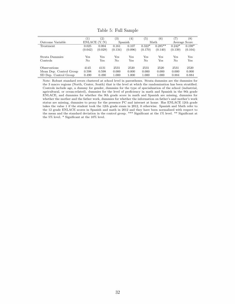
Table 5: Full Sample

(1) (2) (3) (4) (5) (6) (7) (8)Outcome Variable ENLACE (Y/N) Spanish Math Average ScoreTreatment 0.025 0.004 0.161 0.107 0.322* 0.285** 0.242* 0.198*

(0.042) (0.029) (0.134) (0.096) (0.170) (0.140) (0.139) (0.104)

Strata Dummies Yes Yes Yes Yes Yes Yes Yes YesControls No Yes No Yes No Yes No Yes

Observations 4145 4131 2531 2520 2531 2520 2531 2520Mean Dep. Control Group 0.598 0.598 0.000 0.000 0.000 0.000 0.000 0.000SD Dep. Control Group 0.490 0.490 1.000 1.000 1.000 1.000 0.884 0.884

Note: Robust standard errors clustered at school level in parentheses. Strata dummies are the dummies forthe 3 macro regions (North, Center, South) that is the level at which the randomization has been stratified.Controls include age, a dummy for gender, dummies for the type of specialization of the school (industrial,agricultural, or ocean-related), dummies for the level of proficiency in math and Spanish in the 9th gradeENLACE, and dummies for whether the 9th grade score in math and Spanish are missing, dummies forwhether the mother and the father work, dummies for whether the information on father’s and mother’s workstatus are missing, dummies to proxy for the presence PC and internet at home. Has ENLACE 12th gradetakes the value 1 if the student took the 12th grade exam in 2012, 0 otherwise. Spanish and Math refer tothe 12 grade ENLACE scores in Spanish and math in 2012 and they have been normalized with respect tothe mean and the standard deviation in the control group. *** Significant at the 1% level. ** Significant atthe 5% level. * Significant at the 10% level.

32

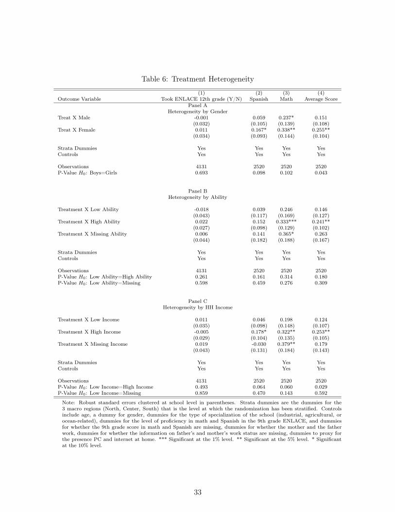
Table 6: Treatment Heterogeneity

(1) (2) (3) (4)Outcome Variable Took ENLACE 12th grade (Y/N) Spanish Math Average Score

Panel AHeterogeneity by Gender

Treat X Male -0.001 0.059 0.237* 0.151(0.032) (0.105) (0.139) (0.108)

Treat X Female 0.011 0.167* 0.338** 0.255**(0.034) (0.093) (0.144) (0.104)

Strata Dummies Yes Yes Yes YesControls Yes Yes Yes Yes

Observations 4131 2520 2520 2520P-Value H0: Boys=Girls 0.693 0.098 0.102 0.043

Panel BHeterogeneity by Ability

Treatment X Low Ability -0.018 0.039 0.246 0.146(0.043) (0.117) (0.169) (0.127)

Treatment X High Ability 0.022 0.152 0.333*** 0.241**(0.027) (0.098) (0.129) (0.102)

Treatment X Missing Ability 0.006 0.141 0.365* 0.263(0.044) (0.182) (0.188) (0.167)

Strata Dummies Yes Yes Yes YesControls Yes Yes Yes Yes

Observations 4131 2520 2520 2520P-Value H0: Low Ability=High Ability 0.261 0.161 0.314 0.180P-Value H0: Low Ability=Missing 0.598 0.459 0.276 0.309

Panel CHeterogeneity by HH Income

Treatment X Low Income 0.011 0.046 0.198 0.124(0.035) (0.098) (0.148) (0.107)

Treatment X High Income -0.005 0.178* 0.322** 0.253**(0.029) (0.104) (0.135) (0.105)

Treatment X Missing Income 0.019 -0.030 0.379** 0.179(0.043) (0.131) (0.184) (0.143)

Strata Dummies Yes Yes Yes YesControls Yes Yes Yes Yes

Observations 4131 2520 2520 2520P-Value H0: Low Income=High Income 0.493 0.064 0.060 0.029P-Value H0: Low Income=Missing 0.859 0.470 0.143 0.592

Note: Robust standard errors clustered at school level in parentheses. Strata dummies are the dummies for the3 macro regions (North, Center, South) that is the level at which the randomization has been stratified. Controlsinclude age, a dummy for gender, dummies for the type of specialization of the school (industrial, agricultural, orocean-related), dummies for the level of proficiency in math and Spanish in the 9th grade ENLACE, and dummiesfor whether the 9th grade score in math and Spanish are missing, dummies for whether the mother and the fatherwork, dummies for whether the information on father’s and mother’s work status are missing, dummies to proxy forthe presence PC and internet at home. *** Significant at the 1% level. ** Significant at the 5% level. * Significantat the 10% level.

33

Table 7: Impact on Self-reported Effort

(1) (2) (3) (4)Full Sample Gender Ability HH Income

Treat 0.240***(0.027)

Treat X Male 0.110(0.094)

Treat X Female 0.349***(0.060)

Treat X Low Ability 0.297 ***(0.080)

Treat X High Ability 0.156*(0.082)

Treat X Missing Ability 0.194(0.161)

Treat X Low Income 0.222 ***(0.078)

Treat X High Income 0.303 ***(0.071)

Treat X Missing Income 0.054(0.174)

Strata Dummies Yes Yes Yes YesControls Yes Yes Yes Yes

Observations 724 724 724 724Mean Dep. Control Group -0.000SD Dep. Control Group 1.000P-Value H0: Boys=Girls 0.071P-Value H0: Low Ability=High Ability 0.359P-Value H0: Low Ability=Missing 0.526P-Value H0: Low Income=High Income 0.477P-Value H0: Low Income=Missing 0.320

Note: Robust standard errors clustered at school level in parentheses. Strata dummies arethe dummies for the 3 macro regions (North, Center, South) that is the level at which therandomization has been stratified.Strata dummies are the dummies for the 3 macro regions(North, Center, South) that is the level at which the randomization has been stratified. Con-trols include age, a dummy for gender, dummies for the type of specialization of the school(industrial, agricultural, or ocean-related), dummies for the level of proficiency in math andSpanish in the 9th grade ENLACE, and dummies for whether the 9th grade score in mathand Spanish are missing, dummies for whether the mother and the father work, dummies forwhether the information on father’s and mother’s work status are missing, dummies to proxyfor the presence PC and internet at home. The self-reported effort has been standardized withrespect to the mean and the standard deviation in the control group. *** Significant at the1% level. ** Significant at the 5% level. * Significant at the 10% level.

34

Table 8: Effect on Perceived Earnings

(1) (2) (3)Less than 4,000 Between 4,000 and 7,000 Above 7,000

Treat X Male -0.171*** 0.005 0.155 ***(0.051) (0.034) (0.047)

Treat X Female -0.102 0.072 *** 0.023(0.067) (0.023) (0.054)

Strata Dummies Yes Yes YesControls Yes Yes Yes

Observations 726 726 726Mean Dep. Control Group 0.338 0.287 0.375SD Dep. Control Group 0.475 0.454 0.486P-Value H0: Boys=Girls 0.163 0.103 0.018

Note: Robust standard errors clustered at school level in parentheses. Strata dummies arethe dummies for the 3 macro regions (North, Center, South) that is the level at which therandomization has been stratified. Controls include age, a dummy for gender, dummiesfor the type of specialization of the school (industrial, agricultural, or ocean-related),dummies for the level of proficiency in math and Spanish in the 9th grade ENLACE,and dummies for whether the 9th grade score in math and Spanish are missing, dummiesfor whether the mother and the father work, dummies for whether the information onfather’s and mother’s work status are missing, dummies to proxy for the presence PC andinternet at home. The dummy Less than $4,000 MX takes the value 1 for an expectedmonthly earning below $4,000 MX upon finishing upper secondary, 0 otherwise. Thedummy Between $4,000 MX and $7,000 MX takes the value 1 for an expected monthlyearning between $4,000 MX and $7,000 MX upon finishing upper secondary, 0 otherwise.The dummy More than $7,000 MX takes the value 1 for an expected earning above$7,000 MX upon finishing upper secondary, 0 otherwise. *** Significant at the 1% level.** Significant at the 5% level. * Significant at the 10% level.

Table 9: Subtrack Distribution

Boys GirlsControl Treatment Total Control Treatment Total

(1) (2) (3) (4) (5) (6)

None 21.64% 17.87% 19.35% 20.90% 22.22% 21.75%Physics and Mathematics 48.51% 47.83% 48.09% 29.10% 25.51% 26.79%Chemistry and Biology 13.43% 12.08% 12.61% 31.34% 16.87% 22.02%Economics and Administration 16.42% 22.22% 19.94% 18.66% 35.39% 29.44%

Observations 134 207 341 134 243 377

K-S Test=0.059 p-value = 0.95 K-S Test=0.167 p-value = 0.016

Note: The bottom line reports the Kolmogorov Smirnov test, and the p-value for the null hypothesis of equality ofdistributions.

35

Table10

:Und

erstan

ding

GenderDifferences:

theRoleof

Tim

ePreferences

(1)

(2)

Self-Rep

ortedEffo

rtAverage

Score

FullSa

mple

FullSa

mple

Treat

XHighDiscoun

t0.011

0.140

(0.125)

(0.113

)Treat

XLow

Discoun

t0.277***

0.204*

(0.033)

(0.107

)

Strata

Dum

mies

Yes

Yes

Con

trols

Yes

Yes

Observation

s713

2500

Propo

rtionof

girlswithHighDiscoun

t0.148

Propo

rtionof

boys

withHighDiscoun

t0.195

P-Value

H0Low

Discoun

t=HighDiscoun

t0.054

0.354

Note:

Rob

uststan

dard

errors

clusteredat

scho

ollevelin

parentheses.

Strata

dum-

miesarethedu

mmiesforthe3macro

region

s(N

orth,Center,

South)

that

isthe

levelat

which

therand

omizationha

sbe

enstratified.Strata

dummiesarethedu

m-

miesforthe3macro

region

s(N

orth,Center,

South)

that

isthelevelat

which

therand

omizationha

sbe

enstratified.

Con

trolsinclud

eage,

adu

mmyforgend

er,

dummiesforthetype

ofspecializ

ation

ofthescho

ol(ind

ustrial,

agricultural,or

ocean-related),du

mmiesforthelevelof

profi

ciency

inmath

and

Span

ish

inthe

9thgrad

eENLACE,an

ddu

mmiesforwhether

the9thgrad

escorein

mathan

dSp

anisharemissing

,du

mmiesforwhether

themotheran

dthefather

work,

dum-

miesforwhether

theinform

ationon

father’san

dmother’sworkstatus

aremissing

,du

mmiesto

prox

yforthepresence

PC

andinternet

atho

me.

The

dummy

Low

Tim

eD

isco

unttakesthevalue1if

therespon

dent

wou

ldbe

willingto

reno

unce

$3,000

MX

toda

yin

orderto

receiveahigh

eram

ount

inthefuture,0otherw

ise.

The

dummy

Hig

hT

ime

Dis

coun

tisdefin

edas

theop

posite

ofLo

wT

ime

Dis

coun

t.***Sign

ificant

atthe1%

level.

**Sign

ificant

atthe5%

level.

*Sign

ificant

atthe

10%

level.

36

Table11

:Add

itiona

lExp

lana

tion

sfortheGenderDifferential:Te

acheran

dParentalB

ehav

iour

(1)

(2)

(3)

(4)

(5)

(6)

OutcomeVariable

MathTeacher

MathTeacher

MathTeacher

Parents

Parents

Parents

solves

doub

tsgivesexercises

invo

lves

stud

ents

mon

itor

attend

ance

mon

itor

grad

esmon

itor

homew

ork

Treat

XMale

0.003

0.050

0.071

-0.036

0.009

-0.039

(0.043)

(0.042)

(0.045)

(0.039)

(0.036)

(0.047)

Treat

XFe

male

-0.003

-0.093

-0.061

0.004

-0.053

-0.054

(0.043)

(0.074)

(0.063)

(0.020)

(0.034)

(0.046)

Strata

Dum

mies

Yes

Yes

Yes

Yes

Yes

Yes

Con

trols

Yes

Yes

Yes

Yes

Yes

Yes

Observation

s727

727

725

728

728

727

MeanDep.Con

trol

Group

forGirls

0.846

0.723

0.346

0.759

0.847

0.569

MeanDep.Con

trol

Group

forBoys

0.860

0.69

10.331

0.765

0.846

0.593

P-Value

H0:Girls=Boy

s0.845

0.119

0.158

0.340

0.178

0.829

Note:

Rob

uststan

dard

errors

clusteredat

scho

ollevelin

parentheses.

Strata

dummiesarethedu

mmiesforthe3macro

region

s(N

orth,Center,

South)

that

isthelevelat

which

therand

omizationha

sbe

enstratified.Strata

dummiesarethedu

mmiesforthe3macro

region

s(N

orth,Center,

South)

that

isthelevelat

which

therand

omizationha

sbe

enstratified.

Con

trolsinclud

eage,

adu

mmyforgend

er,du

mmiesforthetype

ofspecializ

ationof

thescho

ol(ind

ustrial,agricultural,o

rocean-related),d

ummiesforthelevelo

fprofi

ciency

inmathan

dSp

anishin

the9thgrad

eENLACE,a

nddu

mmiesforwhether

the9thgrad

escorein

mathan

dSp

anisharemissing

,du

mmiesforwhether

themotheran

dthefather

work,

dummiesforwhe

ther

theinform

ationon

father’s

andmother’sworkstatus

aremissing

,du

mmiesto

proxyforthepresence

PC

andinternet

atho

me.

The

dummy

Mat

hTea

cher

give

sex

erci

ses

takesthevalue1ifthestud

entrepo

rtsthat

themathteachergivesexercisesto

assess

her/hiscomprehension

,0otherw

ise.

The

dummy

Mat

hTea

cher

invo

lves

stud

ents

takesthevalue1ifthestud

entrepo

rtsthat

themathteacherinvo

lves

stud

ents

during

theclass,

0otherw

ise.

The

dummies

Par

ents

mon

itor

atte

ndan

ce,Par

ents

mon

itor

grad

es,Par

ents

mon

itor

hom

ewor

kstake

thevalue1ifstud

ents

repo

rttheirpa

rentsmon

itor

attend

ance,grad

es,

homew

orkrespectively,0otherw

ise***Sign

ificant

atthe1%

level.**

Sign

ificant

atthe5%

level.*Sign

ificant

atthe10%

level.

37

Figure AI: Baseline Monthly Expected Earnings (Average) upon finishing UpperSecondary

.05

.15

.25

.35

.45

.55

.65

.75

.85

4000

or le

ss

4001

-7000

7001

-1000

0

1000

1-150

00

1500

1-200

00

2000

0 or m

ore

Control TreatmentObserved

Boys

.05

.15

.25

.35

.45

.55

.65

.75

.85

4000

or le

ss

4001

-7000

7001

-1000

0

1000

1-150

00

1500

1-200

00

2000

0 or m

ore

Control TreatmentObserved

Girls

Note: The red line is in correspondence with the statistic provided to the students in the treatment group, andit is equal to the average monthly earning for high school graduates aged between 30 and 40 using data fromENOE second quarter of 2009. The observed distribution is based on data from the ENOE second quarter of 2009.The baseline expected earnings for the average person upon finishing upper secondary were elicited as part of thebaseline survey conducted in November 2009.

38

Table AI: Comparing Characteristics ofMatched and Unmatched Observations

Matched Unmatched p-valueM=U

(1) (2) (3)

Age 16.4 16.7 0.000(0.665) (1.27)

People in the hh 5.17 5.3 0.033(1.74) (1.78)

Father works 0.934 0.949 0.110(0.248) (0.221)

Mother works 0.482 0.457 0.229(0.5) (0.498)

Father with primary 0.302 0.305 0.917(0.459) (0.461)

Mother with primary 0.319 0.334 0.502(0.466) (0.472)

Father with secondary 0.36 0.385 0.354(0.48) (0.487)

Mother with secondary 0.394 0.435 0.108(0.489) (0.496)

Father with hs or higher 0.338 0.31 0.194(0.473) (0.463)

Mother with hs or higher 0.287 0.231 0.005(0.453) (0.422)

Heater at Home 0.638 0.609 0.352(0.481) (0.488)

Washing Machine 0.79 0.778 0.581(0.408) (0.416)

PC at Home 0.577 0.522 0.029(0.494) (0.5)

Internet at Home 0.417 0.344 0.003(0.493) (0.475)

Hours for homeworks 5.49 5.26 0.305(5.86) (5.48)

School days missed 2.68 2.72 0.755(2.36) (2.36)

Sec. school qualification 8.51 8.38 0.003(0.82) (0.801)

Failed subject 0.223 0.227 0.004(0.416) (0.448)

Note: We report the mean of each variable, and its standarddeviation in parentheses. Matched takes the value 1 if thestudent could be matched with the 2009 ENLACE results, 0otherwise. The p-value on the test of equality is based onan OLS regression of the outcome of interest regressed on thematch dummy

39

Table AII: Covariates Balance for different levels of ability

Math 9th Insuff Math 9th Suff or more Math 9th MissingT C p-value T C p-value T C p-value

T=C T=C T=C(1) (2) (3) (4) (5) (6) (7) (8) (9)

Panel A: Survey VariablesAge 16.5 16.5 0.765 16.4 16.3 0.861 16.8 16.7 0.573

(0.721) (0.705) (0.6) (0.617) (1.53) (1.01)People in the hh 5.28 5.3 0.636 5 5.12 0.620 5.28 5.31 0.631

(1.92) (1.94) (1.51) (1.56) (1.83) (1.74)Father works 0.942 0.926 0.196 0.942 0.925 0.230 0.949 0.948 0.877

(0.234) (0.262) (0.234) (0.264) (0.22) (0.222)Mother works 0.49 0.482 0.857 0.495 0.459 0.341 0.495 0.429 0.120

(0.5) (0.5) (0.5) (0.499) (0.501) (0.495)Father with primary 0.333 0.349 0.746 0.243 0.295 0.384 0.292 0.315 0.354

(0.472) (0.477) (0.429) (0.456) (0.455) (0.465)Mother with primary 0.338 0.367 0.531 0.265 0.314 0.424 0.32 0.345 0.355

(0.473) (0.482) (0.442) (0.464) (0.467) (0.476)Father with secondary 0.383 0.369 0.747 0.348 0.341 0.796 0.359 0.403 0.507

(0.486) (0.483) (0.477) (0.475) (0.48) (0.491)Mother with secondary 0.409 0.39 0.742 0.373 0.408 0.240 0.401 0.46 0.226

(0.492) (0.488) (0.484) (0.492) (0.491) (0.499)Father with hs or higher 0.284 0.282 0.919 0.409 0.364 0.508 0.349 0.282 0.098

(0.451) (0.45) (0.492) (0.481) (0.477) (0.45)Mother with hs or higher 0.253 0.243 0.668 0.362 0.278 0.206 0.278 0.195 0.012

(0.435) (0.429) (0.481) (0.448) (0.449) (0.396)Heater at Home 0.639 0.577 0.539 0.704 0.621 0.181 0.626 0.597 0.437

(0.481) (0.494) (0.457) (0.485) (0.485) (0.491)Washing Machine 0.77 0.766 0.946 0.825 0.791 0.645 0.78 0.776 0.624

(0.421) (0.423) (0.38) (0.407) (0.415) (0.417)PC at Home 0.528 0.487 0.530 0.676 0.598 0.252 0.596 0.465 0.029

(0.5) (0.5) (0.468) (0.491) (0.491) (0.499)Internet at Home 0.369 0.35 0.737 0.512 0.419 0.285 0.432 0.276 0.006

(0.483) (0.477) (0.5) (0.494) (0.496) (0.447)Hours for homeworks 5.44 5.33 0.995 5.52 5.68 0.997 5.56 5.03 0.283

(6.47) (6.13) (5.25) (5.62) (6.08) (4.98)School days missed 2.89 3.08 0.435 2.13 2.51 0.044 2.75 2.69 0.727

(2.57) (2.67) (1.74) (2.16) (2.48) (2.27)Sec. school qualification 8.27 8.21 0.296 8.79 8.72 0.627 8.42 8.36 0.308

(0.768) (0.769) (0.763) (0.812) (0.82) (0.785)Failed subject in sec. 0.293 0.277 0.676 0.159 0.173 0.758 0.258 0.291 0.265

(0.455) (0.448) (0.366) (0.379) (0.438) (0.455)

Note: We report the mean of each variable, and its standard deviation in parentheses. The p-value on the test ofequality is based on an OLS regression of the outcome of interest regressed on the treatment dummy and the stratadummies, with standard errors clustered at school level.

40