Cleaning the Bathwater with the Baby:The Health Co-Benefits of Carbon

Pricing in Transportation

Christopher R. Knittel and Ryan Sandle

August 2011 CEEPR WP 2011-015

A Joint Center of the Department of Economics, MIT Energy Initiative and MIT Sloan School of Management.

Cleaning the Bathwater with the Baby:

The Health Co-Benefits of Carbon Pricing in Transportation

Christopher R. Knittel and Ryan Sandler∗

August 23, 2011

Abstract

Efforts to reduce greenhouse gas emissions in the US have relied on Corporate Average Fuel

Economy (CAFE) Standards and Renewable Fuel Standards (RFS). Economists often argue

that these policies are inefficient relative to carbon pricing because they ignore existing vehicles

and do not adequately reduce the incentive to drive. This paper presents evidence that the

net social costs of carbon pricing are significantly less than previous thought. The bias arises

from the fact that the demand elasticity for miles travelled varies systematically with vehicle

emissions; dirtier vehicles are more responsive to changes in gasoline prices. This is true for

all four emissions for which we have data—nitrogen oxides, carbon monoxide, hydrocarbon,

and greenhouse gases—as well as weight. This reduces the net social costs associated with

carbon pricing through increasing the co-benefits. Accounting for this heterogeneity implies

that the welfare losses from $1.00 gas tax, or a $110 per ton of CO2 tax, are negative over the

period of 1998 to 2008 even when we ignore the climate change benefits from the tax. Co-benefits

increase by over 60 percent relative to ignoring the heterogeneity that we document. In addition,

accounting for this heterogeneity raises the optimal gas tax associated with local pollution, as

calculated by Parry and Small (2005), by as much as 57 percent. While our empirical setting is

California, we present evidence that the effects may be larger for the rest of the US.

∗This paper has benefited from conversations with Severin Borenstein, Michael Greenstone, Jonathan Hughes,Dave Rapson, Nicholas Sanders, and Catherine Wolfram. We gratefully acknowledge financial support from theUniversity of California Center for Energy & Environmental Economics and the Sustainable Transportation Centerat UC Davis. A portion of the paper was written while Knittel was a visitor at the Energy Institute at Haas.Knittel: William Barton Rogers Professor of Energy Economics, Sloan School of Management, MIT and NBER, email:knittel@mit.edu. Sandler: Department of Economics, University of California, Davis, email: rsandler@ucdavis.edu.

1 Introduction

As concerns about climate change grow, so have debates about what policy tools to use to reduce

emissions. The transportation sector accounts for nearly 37 percent of US greenhouse gas (GHG)

emissions; it has therefore seen a number of policy changes during the past two decades. Within

the transportation industry, greenhouse gas pricing, via either a carbon tax or cap & trade system,

has succumbed to Corporate Average Fuel Economy (CAFE) standards to increase the new vehicle

fleet fuel economy and the Renewable Fuel Standard (RFS) to decrease the carbon intensity of

fuels. Economists have long viewed these policies with derision, arguing instead for the merits of

Pigouvian taxes.

A large literature exists showing the inefficiency, relative to gasoline or carbon taxes, associated

with both CAFE and the RFS. For the RFS, the main sources of inefficiency are that the policy

over-incentivizes marginally cleaner fuels and suppresses fuel prices. CAFE, on the other hand,

ignores the existing fleet and reduces the marginal cost of driving, increasing the number of miles

driven. For example, Holland et al. (2011) find that even in the long run GHG reductions under

the RFS are nearly three times more costly than equivalent reduction under a cap & trade system,

while Jacobsen (2011) finds that CAFE standards are nearly seven times more costly than gasoline

taxes in reducing GHG emissions.

In this paper we argue that the net social cost of GHG taxes have been overstated. The source

of this bias comes from the heterogeneity in how different types of vehicles, in terms of the other

externalities associated with driving, respond to changes in gasoline prices. We show that vehicles

with higher externalities, both in terms of local pollution and weight, respond more to gasoline

prices. This is true for all three vehicle emissions for which we have data: carbon monoxide,

hydrocarbons, and nitrogen oxides. It is also true for vehicle weight and greenhouse gases. This

heterogeneity increases the co-benefits associated with a greenhouse gas tax from reductions in

criteria pollutants.1

We find that the average “two-year” elasticity is 0.26 across all vehicles, but the ratio of the

elasticity for the dirtiest quarter of vehicles with the cleanest quarter of vehicles is 4.7, 4.5, and

3.4 for carbon monoxide, hydrocarbons, and nitrogen oxides, respectively. The ratio is 1.6 for

1Criteria air pollutants are the only air pollutants for which the Administrator of the U.S. Environmental Protec-tion Agency has established national air quality standards defining allowable ambient air concentrations. Congresshas focused regulatory attention on these pollutants (i.e., carbon monoxide, lead, nitrogen dioxide, ozone, particulatematter, and sulfur dioxide) because they endanger public health and they are widespread throughout the U.S.

1

greenhouse gases and 1.2 for vehicle weight. We also estimate how the hazard rate of scrapping a

vehicle varies with criteria pollutant emissions. Here, the evidence is more mixed.

We use these estimates to simulate the co-benefits from a carbon tax. For each vehicle in

our data, we calculate the change in miles driven from the tax and the change in the vehicle’s

probability of survival and the resulting change in vehicle emissions. We do this across our entire

time period and in each year. We then quantify these reductions using the estimated marginal

damages in Muller and Mendelsohn (2009) and Matthews and Lave (2000). We find that once

the heterogeneous response is accounted for, there is essentially no change in near-term consumer

surplus from a $110 CO2 tax from 1998 to 2008; the welfare near-term co-benefits are nearly 20

percent greater than the change in consumer surplus from the tax increase. If one fails to account

for the heterogenous response, the simulated co-benefits fall to 74 percent of the consumer welfare

loss from the tax. We discuss reasons why these effects should be interpreted as strict lower bounds.

Given that the vehicle fleet has, over time, become cleaner in terms of criteria pollutant emis-

sions, we find that the co-benefits have fallen over our sample, but remain substantial even at the

end. Early in the sample, we simulate that consumers would have been better off from the tax,

with the co-benefits being twice as large as the welfare losses from the tax. In the last year of

our sample, the co-benefits fall to 55 percent of the welfare losses from the tax. We argue that

these are still substantial, reducing the cost per ton of carbon saved from $83 to $23. Again, not

accounting for heterogeneity implies a net cost nearly twice as large as the net cost accounting for

heterogeneity in the final year of our sample.

To put these numbers into context, Greenstone, Kopits, and Wolverton (2011) estimate the

social cost of carbon for a variety of assumptions about the discount rate, relationship between

emissions and temperatures, and models of economic activity. For 2010, using a 3 percent discount

rate, they find an average SCC of $21.40, with a 95th percentile of $64.90. Using a 2.5 percent

discount rate, the average SCC is $35.10. Our results suggest that once the co-benefits are accounted

for, a $1.00 gas tax (i.e., a $110 per ton of CO2 tax) would be nearly cost-effective even at the

lower of these three numbers.2

Our results also have implications for the optimal gas tax in the presence of multiple market

failures. Parry and Small (2005) calculate that the optimal gasoline tax within the US accounting

for local and global pollution, accidents, congestion, and inefficiencies associated with income taxes.

2Of course, a tax somewhere below this would likely maximize welfare.

2

They find that the optimal tax is $1.01 in the US, while it is $1.62 in the UK. We calculate the

optimal gas tax for California with and without heterogeneity; with heterogeneity the optimal tax

increases from $0.92 to $1.05 in 1998 and from $0.85 to $0.90 in 2008. The relatively small increase

is due, in large part, to the fact that the Pigouvian tax associated with congestion dominates the

tax. The portion of the optimal tax attributed to local pollution increases from $0.22 to $0.33 in

1998 and from $0.08 to $0.13 in 2008, a change of 52 and 57 percent, respectively.

We argue that these results should be viewed as strict lower bounds of the co-benefits for a

variety of reasons. First, we have ignored all other negative externalities associated with vehicles;

many of these, such as particulate matter, accidents, and congestion externalities, will be strongly

correlated with VMT and the emissions of NOx, HCs, and CO. Second, because of the rules of

the California Smog Check program, from which our data come from, many vehicles that were

produced prior to standards on emissions are not required to be tested, leading to their omission

in this analysis. Third, a variety of behavior associated with smog check programs would lead

the on-road emissions of vehicles to likely be higher than the tested levels. These include, but are

not limited to: fraud, tampering with emission-control technologies between tests, failure to repair

emission-control technologies until a test is required, etc.

We also present evidence that, while the marginal damages from NOx and HCs are larger

within California, Californian vehicles are, on average, much cleaner that the rest of the US. We

show, using county-level data from the EPA on average vehicle emission rates, that the county-level

average per-mile externalities are roughly 30 percent lower in California compared to the rest of

the US. Therefore, while are unable to estimate elasticities outside of California, this suggests that

provided the heterogeneity is somewhat similar to what we observe in California, the co-benefits

may be larger for other states.

Finally, we also investigate several sources of the heterogeneity. At the most general level, we

show that while the age of the vehicle is a major driver in our results—older vehicles respond

more to changes in gasoline prices—this does not explain all of the heterogeneity. There are at

least two additional sources of criteria pollutant-related heterogeneity in the response of changes in

gasoline prices. For one, income may be correlated with criteria pollutant emissions, and driving

the difference. Second, it may come from within-household shifts in vehicles miles travelled, for

example if a household has one newer and one older vehicle. As gas prices increase, they may shift

miles away from the older vehicle and to the newer vehicle. Because age is, on average, correlated

3

with both greenhouse gas and criteria pollutant emissions, this would lead to our result. Our data

can speak to this. We find that while there is evidence of both a within household effect and an

income effect, a significant amount of variation persists once these are accounted for.

We bring together a number of unique data sets. The first is the universe of test records for

California’s emissions inspection and maintenance program, Smog Check, for the period of 1996 to

2010. California requires vehicles older than six years to receive biennial testing. In addition, testing

occurs each time a vehicle changes ownership and randomly for a small share of vehicles. Among

other things, the inspection data report odometer readings, which we use to measure vehicle miles

travelled between tests. The tests also measure criteria pollutant emissions. To measure greenhouse

gas emissions, we link these data to EPA fuel economy ratings. In addition, the data are linked to

EIA gas prices for the same years. For roughly 75 percent of the smog check records, we are able to

link them to Department of Motor Vehicle address recordings. This allows us to aggregate vehicles

to households, as well as match vehicles with Census tract demographic data. Finally, to capture

scrappage decisions we use CARFAX data for roughly 32 million vehicles that track the last date

a vehicle was recorded within the US or exported to a foreign country.

The paper proceeds as follows. Section 2 discusses the empirical setting. The data are discussed

in Section 3. Section 4 provides graphical support for the empirical results. Sections 5 and 6 present

empirical models and results on miles driven and scrappage . Section 7 presents the results from

the two policy simulations. Section 8 discusses how our results apply to regions of the US outside

of California. Finally, Section 9 concludes the paper.

2 Empirical Setting

Our empirical setting is California. California implemented its first inspection and maintenance

program in 1984 in response to the 1977 Clean Air Act Amendments. The initial incarnation of

the Smog Check program relied purely on a decentralized system of privately run, state-licensed

inspection stations, and was plagued by cheating and lax inspections. Although the agreement

between California and the federal EPA promised reductions in hydrocarbon and carbon monoxide

emissions of more the 25 percent, estimates of actual reductions of the early Smog Check Program

range from zero to half that amount (Glazer, Klein, and Lave (1995)).

The 1990 Clean Air Act Amendments required states to implement an enhanced inspection and

maintenance program in areas with serious to extreme non-attainment of ozone limits. Several of

4

California’s urban areas fell into this category, and in 1994, a redesigned inspection program was

passed by California’s legislature after reaching a compromise with the EPA. The program was

updated in 1997 to address consumer complaints, and fully implemented by 1998. Among other

improvements, California’s new program introduced a system of centralized “Test-Only” stations

and an electronic transmission system for inspection reports.3 Today, more than a million Smog

Checks take place each month.

An automobile appears in the data for a number of reasons. First, vehicles that are older than

four years old must pass a smog check within 90 days of any change in ownership. Second, in parts

of the state (details below) an emissions inspection is required every other year as a pre-requisite

for renewing the registration on a vehicle that is six years old or older. Third, a test is required if

a vehicle moves from out-of-state. Vehicles which fail an inspection must be repaired and receive

another inspection before they can be registered and driven in the state. There is also a group

of exempt vehicles. These are: vehicles of 1975 model-year or older, hybrid and electric vehicles,

motorcycles, diesel powered vehicles, and large trucks powered by natural gas.

Since 1998, the state has been divided into three inspection regimes (recently expanded to

four), the boundaries of which roughly correspond to the jurisdiction of the regional Air Quality

Management Districts. “Enhanced” regions, designated because they fail to meet state or federal

standards for carbon monoxide (CO) and ozone, fall under the most restrictive regime. All of the

state’s major urban centers are in Enhanced areas, including the greater Los Angeles, San Francisco,

and San Diego metropolitan areas. Vehicles registered to an address in an Enhanced area must pass

a biennial Smog Check in order to be registered, and they must take the more rigorous Acceleration

Simulation Mode (ASM) test. The ASM test involves the use of a dynamometer, and allows for

measurement of NOx emissions. In addition, a randomly selected two percent sample of all vehicles

in these areas is directed to have their Smog Checks at Test-Only stations, which are not allowed

to make repairs.4 Vehicles which match a “High Emitter Profile” are also directed to Test-Only

stations, as are vehicles which are flagged as “gross polluters” (this occurs when a vehicle fails an

inspection with twice the legal limit of one or more pollutant in its emissions). More recently some

“Partial-Enhanced” areas have been added, where a biennial ASM test is required, but no vehicles

are directed to Test-Only stations.

3For more detailed background see http://www.arb.ca.gov/msprog/smogcheck/july00/if.pdf.4Other vehicles can be taken to Test-Only stations as well if the owner chooses, although they must get repairs

elsewhere if they fail.

5

Areas with poor air quality that does not exceed legal limits fall under the Basic regime. Cars

in a Basic area must have biennial Smog Checks as part of registration, but they are allowed to

take the simpler Two Speed Idle (TSI) test, and no vehicles are directed to Test-Only stations. The

least restrictive regime, consisting of rural mountain and desert counties in the east and north of

the state, is known as the Change of Ownership area. As the name suggests, inspections in these

areas are only required upon change of ownership; no biennial Smog Check is required.

2.1 Automobiles, Criteria Pollutants, and Health

The tests report the emissions of three criteria pollutant: Nitrogen oxides, hydrocarbon, and carbon

monoxide. All three of these pollutants are a direct consequences of the combustion process within

either gasoline or diesel engines. Both NOx and HCs are precursors to ground-level ozone, but, as

with CO, have been shown to have negative health effects individually.5

While numerous studies have found links between the exposure of either smog or these three pol-

lutants directly and health outcomes, the direct mechanisms are still uncertain. These pollutants,

as well as smog, may directly impact vital organs or indirectly cause trauma. For example, CO

can bind to hemoglobin, thereby decreasing the amount of oxygen in the bloodstream. High levels

of carbon monoxide have also been linked to heart and respiratory problems. On its own, NOx is

also a fine-particle particulate matter (PM). PM has been shown to irritate lung tissue, lowers lung

capacity and hinders long term-lung development. Extremely small PM can be absorbed through

the lung tissue and cause damage on the cellular level. On its own, HC can interfere with oxygen

intake and irritate lungs. Ground-level ozone is a known lung irritant, has been associated with

lowered lung capacity, and can exacerbate existing prior heart problems as well as lung problems

such as asthma or allergies.

3 Data

We bring together a number of large data sets. First, we have the universe of smog checks from 1996

to 2010 from California’s Bureau of Automotive Repair (BAR). These data report the location of

the test, the vehicle’s VIN, odometer reading, the reason for the test, and test results. We decode

the VIN to obtain the vehicles’ make, model, engine, and transmission. Using this, we match the

5CO has also been shown to speed up the smog-formation process. For early work on this, see Westberg, Cohen,and Wilson (1971).

6

vehicles to EPA data on fuel economy. Because the VIN decoding only holds for vehicles made

after 1981, our data are restricted to these models. We also restrict our sample to 1998 and beyond

given the large changes that occurred in the smog check test program in 1997. This yields roughly

120 million observations.

The smog check data report nitrogen oxides and hydrocarbons in terms of parts per million and

carbon monoxide levels as a percentage of the exhaust under two engine revolutions per minute

(RPMs). The more relevant metric is a vehicles emissions per mile. We convert the smog check

reading into emissions per mile using conversion equations developed by Sierra Research for Califor-

nia Air Resources Board for Morrow and Runkle (2005), an evaluation of the Smog Check program.

The conversion equations are functions of all three pollutants, vehicle weight, model year, and truck

status.

We also estimate scrappage decisions. For this we use data from CARFAX Inc for 32 million

of the vehicles in the BAR data. These data report the last date and location a given vehicle was

recorded by CARFAX in the United States, which includes registrations, emissions inspections,

repairs, import/export records and accidents. The CARFAX data do not track vehicles that move

outside of the US; we assume the vehicle continues to be driven if exported.

Finally, at times we use information about the household. For a subsample of our BAR data,

we are able to match vehicles to given households using data come from confidential Department

of Motor Vehicle records that track the registered address of the vehicle. We use this information

to aggregate up to addresses, the stock of vehicles registered. Appendix A discusses how this is

done. These data are from 2000 to 2008.

For vehicles required to get biennial smog checks, we construct the average gasoline price be-

tween the two test data using EIA’s national average prices.

Table 1 reports means and standard deviations of the main variables used in our analysis, as well

as these summary statistics split by vehicle vintage and 1998 and 2008. The average fuel economy

of vehicles in our sample is 23.5 MPG, with fuel economy falling over our sample. The change in

the average dollar per mile has been dramatic, more than doubling over our sample. The dramatic

decrease in vehicle emissions is also clear in the data, with per-mile emissions of hydrocarbon, CO,

and NOx falling considerable from 1998 to 2008. The tightening of standards has also meant that

more vehicles fail the smog check late in the sample, although some of this is driven by the aging

vehicle fleet.

7

4 Preliminary Evidence

One of the main driving forces behind our empirical results is whether vehicle elasticities, both

in terms of their intensive and extensive margins, vary systematically with the magnitude of their

externalities. In this section, we present evidence that:

◦ significant variation exists in terms of vehicle externalities across vehicles within a year,

◦ significant variation exists in terms of vehicle externalities across vehicles across years,

◦ significant variation exists in terms of vehicle externalities within the same make, model,model year, etc. within a year, and

◦ simple statistics, such as the average miles travelled by vehicle type, suggest that elasticitiesare correlated with externalities.

Figure 1 plots the distributions of NOx, HCs, and CO emissions in 1998, 2004, and 2010.

The distribution of criteria pollutant emissions tends to be right-skewed in any given year, with a

standard deviation equal to roughly one to three times the mean, depending on the pollutant. This

implies that there are a vehicles on the road that are quite “dirty” relative to the mean vehicle.

Over time, the distribution has shifted to the left, as vehicles have been getting cleaner, but the

range still remains.

Table 2 reports the means and standard deviations across all vehicles receiving smog checks in a

given year. From 1998 to 2008 the average emissions of NOx, HCs, and CO fell between 65 and 85

percent. However, the standard deviations, relative to the means, have increased over time. This

is especially true for CO, where the standard deviation is over 4 times the mean at the end of the

sample.

This variation is not only driven by the fact that different types of vehicles are on the road in a

given year, but also variation within the same vehicle-type, defined as a make, model, model-year,

engine, number of doors, drivetrain combination. To see this, Figure 2 plots the distributions of

emissions for the most popular vehicle/year in our sample, the 2001 4-door Toyota Corolla in 2009.

The vertical red line is at the mean of the distribution. Here, again, we see that even within the

same vehicle-type in the same year, the distribution is wide and right skewed. The distribution

of hydrocarbons is less skewed, but the standard deviation is 25 percent of the mean. Carbon

monoxide is also less skewed, and has a standard deviation that is 36 percent of the mean. Across

all years and vehicles, the mean emission rate of a given vehicle in a given year, on average, is

roughly four times the standard deviation for all three pollutants (Table 2).

8

To understand how the distribution within a given vehicle changes over time, Figure 3 plots

the distribution of the 1995 3.8L, front-wheel drive, Ford Windstar in 1999, 2001, 2004, and 2007.6

These figures suggest that over time the distributions shift to the right, become more symmetric,

and the standard deviation grows considerably, relative to the mean. Across all vehicles, the ratio

of the mean emission rate of NOx and the standard deviation of NOx has increased from 3.16 in

1998 to 4.53 in 2010. For hydrocarbons, this has increased from 3.59 to 5.51; and, has increased

from 3.95 to 5.72 for CO.

These distributions suggest that there is significant scope for meaningful emissions-correlated

variation in elasticities across vehicles and within the same vehicle-type. We next present suggestive

evidence that this, too, is the case. To do this, we categorize vehicles into four groups, based on

the four quartiles of a given pollutant within a given year. We then plot how the log of daily miles

driven has changed over our sample—a period where gas prices increased from roughly $1.35 to

$3.20.

Figure 4 and 5 foreshadow our results on the intensive margin. Figure 4 plots the median of

daily miles travelled across our sample split up by the emissions quartile of the vehicle. While the

dirtiest quartile begins at a slightly lower daily-VMT, it appears to drop much further than the

other quartiles. Indeed, the there is a general trend of monotonicity across the four emissions. To

see this more clearly, Figure 5 rescales the median VMT in 1998 and plots the average of the log of

VMT over time by quartiles of each pollutant. For each pollutant, the log change in bottom-quartile

vehicles is larger than the first quartile, with the other two quartiles often exhibiting monotonic

changes in miles driven.7

5 Vehicle Miles travelled Decisions

Our first set of empirical models estimates how vehicle miles travelled (VMT) decisions are affected

by changes in gas prices, and how this elasticity varies with vehicle characteristics. Our empirical

approach mirrors Figures 4 to 5. For each vehicle receiving a biennial smog check, we calculate

average daily miles driven and the average gasoline price during the roughly two years between

6We chose this vehicle because the 1995 3.8L, front-wheel drive, Ford Windstar in 1999 is the second most popularentry in our data and it is old enough that we can track it over four 2-year periods.

7Constructing the graphs in this way hides variation in the average level of driving by quartile. We find somevariation in this, with the first or second quartile vehicles being driven more in 1998 for the criteria pollutants. Forfuel economy, the bottom quartile is driven the most in 1998.

9

smog checks. We will then allow the elasticity to vary based on the emissions of the vehicle. We

begin by estimating:

ln(VMTigt) = β ln(DPMigt) + γDtruck +2008∑

k=1998

ωk · time+ µt + µi + µg + µv + εigt (1)

where i indexes vehicle-types, g geographic locations, t time, and v vehicle age, or vintage. DPMigt

is the average dollars per mile of the vehicle between smog checks, Dtruck is an indicator for whether

the vehicle is a truck, and time is a time trend.8

We begin the analysis by including year, vintage, and zip code fixed effects. We then pro-

gressively include finer vehicle-type fixed effects by including make, then make-model-model year-

engine, and ending with specific-vehicle fixed effects.

We next differentiate the influence of gas prices by vehicle attributes related to the magnitude

of their negative externalities—criteria pollutants, CO2 emissions, and weight. We do this in two

ways. First, we split vehicles up by the quartile the vehicle falls into with respect to the within-

year emissions of nitrogen oxides (NOx), hydrocarbons (HC), and carbon monoxide (CO), fuel

economy (CO2), and weight. Second, we include a linear interaction of these variables and the log

of gas prices. Below we investigate, in a semi-parametric way, the actual functional form of this

relationship.

Tables 3 through 7 report the results across externality-type.

Model 1 controls for only the year, vintage of the vehicle, and zip code where the vehicle received

its smog check. Model 2 adds vehicle-make fixed effects. Model 3 includes the quartile interactions

and the quartiles themselves. Model 4 includes VIN x-prefix fixed effects which effectively are

vehicle make/model/model year/drivetrain/engine fixed effects. Model 5 includes VIN fixed effects,

or specific-vehicle fixed effects. Model 6 includes the quartile variables, and Model 7 allows for the

relationship between externality and gas prices to be linear.

Table 3 focuses on nitrogen oxides. Moving from Models 1 to 5 illustrates the importance of

controlling for vehicle-type fixed effects. Initially, the average elasticity falls from 0.399 to 0.140

when including fixed make effects, but then rises when including finer detailed vehicle fixed effects.

Our final specification includes individual vehicle fixed effects yielding an average elasticity of 0.257.9

8Our dollars per mile variable uses the standard assumption that 45 percent of a vehicle miles driven are in thecity and 55 percent are on the highway, along with the vehicles EPA fuel economy ratings.

9This is much larger than that found in Hughes, Knittel, and Sperling (2008) reflecting the longer run nature ofour elasticity.

10

In general, we find that the more finely we control for vehicle-type the larger the heterogeneity in

terms of the dollar-per-mile elasticity, while the average elasticity does not change much once we

control for the vehicle’s make. Focusing on Models 6 and 7, we find large heterogeneity. The DPM-

elasticity for the cleanest vehicles, quartile one, is 0.094, while the DPM-elasticity for the dirtiest

vehicles is over five times this, at 0.323. To put these numbers in context, the average per-mile

NOx emissions of a quartile one vehicle is 0.163 grams, while the average per-mile NOx emissions

of a quartile four vehicle is 1.68 grams. Model 7 assumes the relationship is linear in centiles of

NOx and finds that each percentile increase in the per-mile NOx emission rate is associated with a

change in the elasticity of .003, from a base of 0.078.

We find similar patterns across the three other pollutants. Table 4 reports the results for

hydrocarbons. Here, the elasticity of the cleanest vehicles and the elasticity of the dirtiest vehicles

differ by a factor of 4.5. Table 5 reports the results for carbon monoxide. Here there is almost a 4.7

times difference in the elasticity of the cleanest quartile vehicles and the dirtiest quartile vehicles.

Table 6 reports the results for fuel economy, or CO2 emissions. The lowest quartile here are the

most polluting vehicles. Their elasticity is 1.6 times as large as the cleanest vehicles. It is important

to note that this is not driven by the fact that a given change in gas prices implies a larger change

in the price per miles, since the independent variable is the log of the price per mile.10 The linear

interaction implies that vehicles at the 100th percentile have an average elasticity of roughly zero.

We come back to this below.

While the elasticities are larger for dirtier vehicles, the average miles driven are smaller at

the beginning of the sample for these vehicles. In terms of levels, in 1998 vehicles in the bottom

quartile in terms of NOx emissions are driven 2.23 more miles per day, on average, than vehicles in

the top quartile; they are driven 0.10 and 1.03 miles more per day, on average, than vehicles in the

second and third quartiles, respectively. Vehicles in the bottom quartile in terms of hydrocarbon

emissions are driven 0.95 miles per day less, on average, than vehicles in the second quartile and

3.28 and 4.68 miles more, on average, than vehicles in the third and fourth quartiles, respectively

(in 1998). Vehicles in the bottom quartile in terms of CO emissions are driven 3.00 miles per day

less, on average, than vehicles in the second quartile, and 7.63 and 4.63 miles more, on average, than

vehicles in the third and fourth quartiles, respectively (in 1998). Finally, vehicles in the bottom

quartile in terms of fuel economy are driven 2.44, 2.04, and 1.7 miles per day more, on average,

10Also, note that this does not matter for the models with VIN fixed effects.

11

than vehicles in the second, third, and fourth quartiles, respectively (in 1998). We account for

these differences in the policy simulations below.

Table 7 splits vehicles up into weight quartiles. Here, too, we find that those vehicles with the

largest negative externality, heavier vehicles, are more responsive to changes in gas prices. However,

the heterogeneity is not as stark.

We next investigate the functional forms of these relationships in a semi-parametric way. For

each externality, we define vehicles by their percentile of that externality. We then estimate equation

1 separately for vehicles falling in the zero to first percentile, first to second, etc. Figure 7 plots

a lowess smoothed line through these 100 separate elasticity estimates. For the three criteria

pollutants, we find that the relationship is quite linear with the elasticity being positive for the

cleanest 20 percent of vehicles. The dirtiest vehicles have elasticities that are roughly 0.4. For

fuel economy, the relationship is fairly linear from the 60th percentile onwards, but begins steeply

and flattens out from the 20th percentile to the 40th. The elasticity of the lowest fuel economy

vehicles is nearly 0.6. To put these numbers into context across the different years, the average

fuel economy of the 20th percentile is 18.7, while the average for the 40th percentile is 21.75. The

variation in elasticities across weight is not monotonic. The relationship begins by increasing until

roughly the 20th percentile, and then falls more or less linearly thereafter. The elasticity of the

heaviest vehicles is roughly 0.3.

We next investigate whether the roughly-linear relationship between criteria pollutant emissions

and the elasticity is due to “over smoothing”. Figure 8 plots the lowess smoothed lines under

different bandwidths. The top left figure simply reports the 100 elasticities. There is some evidence

that the relationship is not monotonic early on, but from the 5th percentile on, the relationship

appears monotonic. Doing this exercise for the other criteria pollutants yields similar results.

5.1 The Source of the Heterogeneity

While the co-pollutant benefits accrue regardless of the mechanism behind the heterogeneity, it is

of independent interest to investigate the mechanism. We investigate three sources, which are not

necessarily independent of each other. First, it may be driven entirely through a vintage effect.

That is, older vehicles are both more responsive to changes in gas prices and have higher emissions.

Second, it might be driven by differences in the incomes of consumers that drive dirtier versus

12

cleaner vehicles. Third, it may result from households shifting which of their vehicles are driven in

the face of rising gasoline prices.

To investigate whether it is simply a vintage effect, we redefine the quartiles based on the

distribution of emissions within vintage bins. We split vehicles into three age categories: 4 to 9

years old, 10 to 15 years old, and 16 to 27 years old.

Tables 8 through 11 report the results across externality-type. These results suggest that while

vintage is an important driver in the externality-based heterogeneity, it is not the only source. In

all four externality types variation exists within age bin; furthermore, in all but fuel economy this

variation would appear to be economically significant.

For a sub-sample of our smog check vehicles, we are able to group them into households. This

grouping comes from access to California Department of Motor Vehicles (DMV) data. A number

of steps are undertaken to “clean” the address entries in the DMV records. These are discussed

in Appendix A. Ultimately, however, the subsample of vehicles that we are able to match likely

draw more heavily from households residing in single-family homes. Given this selection, it is not

surprising that we find average elasticities that differ from those presented above. In particular,

they are smaller suggesting that the elasticity may be correlated with income.

The results from this sample are presented in Table 13. For this sample, we construct two

additional variables meant to capture the household stock of vehicles. The variable “Higher MPG

in HH” equals one if there is another vehicle in the household that has a higher MPG rating than

the vehicle at question. Likewise, the variable “lower MPG in HH” equals one if there is another

vehicle in the household that has a lower MPG rating than the vehicle at question.

If household shift usage from low MPG vehicles to high MPG vehicles, we would expect “Higher

MPG in HH” to be negative and “Lower MPG in HH” to be positive. The results suggest that

this is a mechanism, but not the only one. If there is a vehicle with higher fuel economy in the

household, the elasticity is larger, while if there is a vehicle with a lower MPG, the elasticity is

smaller. Column 2 of Table 13 adds these variables to our base specification. The point estimates

suggest that a vehicle in the highest fuel economy quartile belonging to a household that also has

a lower fuel economy vehicle has a near zero elasticity.11

For this same sample of vehicles, we also use the Census-tract information to categorize owners

11The sum of the two vehicle-stock variables is positive, but because lower fuel efficient vehicles are driven moreearlier in the sample, the elasticities are not comparable in terms of what they imply for total miles driven.

13

into income quartiles. We interact these quartiles with the log of dollars per mile to see if differences

in elasticities exist. Column 3 of Table 13 adds these interaction terms. There is some evidence that

higher income consumers are less elastic, but these effects are not enough to reverse the emissions

quartile effects; vehicles in the bottom quartile remain nearly three times more sensitive even after

accounting for income differences.

Our smog check data report the zip code of the testing station the vehicle visited. For our

more general sample, we can also use this information to construct measures of income. Table 14

compares these results with the DMV data. We find similar differences in the elasticities, despite

the larger average elasticity. That is, the average elasticity of the top income quartile vehicles is

roughly 0.03 less elastic, than the bottom quartile, in both samples.

6 Scrappage Decisions

Our next set of empirical models examine how vehicle owners’ decisions to scrap their vehicles are

affected by gasoline prices. Again we will also examine how this effect varies over emissions profiles.

We determine whether a vehicle has been scrapped using the data from CARFAX Inc. We

begin by assuming that a vehicle has been scrapped if more than a year has passed between the

last CARFAX record and the date when CARFAX produced our data extract (October 1, 2010).

However, we treat a vehicle as being censored if the last CARFAX record was not in California, or if

more than a year and a half passed between the last Smog Check in our data and the last CARFAX

record. As well, to avoid treating late registrations as scrappage, we treat all vehicles with Smog

Checks after 2008 as censored. Finally, to be sure we are dealing with scrapping decisions and not

accidents or other events, we only examine vehicles which are at least 10 years old.

Some modifications to our data are necessary. To focus on the long-run response to gasoline

prices, our model is specified in discrete time, denominated in years. Where vehicles have more

than one Smog Check per calendar year, we use the last Smog Check in that year. Also, since it is

generally unlikely that a vehicle is scrapped at the same time as its last Smog Check, we create an

additional observation for scrapped vehicles either one year after the last Smog Check, or 6 months

after the last CARFAX record, whichever is later. For these created observations, odometer is

imputed based on the average VMT between the last two Smog Checks, and all other variables

take their values from the vehicle’s last Smog Check. An exception is if a vehicle fails the last Smog

Check in our data. In this case, we assume the vehicle was scrapped by the end of that year.

14

Because many scrapping decisions will not take place until after our data ends, a hazard model

is needed to deal with right censoring. Let Tjivg be the year in which vehicle j, of vehicle type i,

vintage v, and geography g is scrapped. Assuming proportional hazards, our basic model is:

Pr[t < Tjivg < t+ 1|T > t] = h0iv(t) · exp{βxDPMgt + γDfailjt

+ ψGjgt + αXjt},

where DPMgt is defined as before, Dfailjtis a dummy equal to one if the vehicle failed a Smog

Check any time during year t, G is a vector of demographic variables, determined by the location

of the Smog Check, X is a vector of vehicle characteristics, including a dummy for truck and a

6th-order polynomial in odometer, and h0jiv(t) is the baseline hazard rate, which varies by time but

not the other covariates. In some specifications, we will allow each vehicle type and vintage to have

its own baseline hazard rate.

We estimate this model using semi-parametric Cox proportional hazards regressions, leaving

the baseline hazard unspecified. We report exponentiated coefficients, which may be interpreted as

hazard ratios. For instance, a 1 unit increase in DPM will multiply the hazard rate by exp{β}, or

increase by (exp{β}−1) percent. In practice, we scale the coefficients on DPM for a 5-cent change,

corresponding to a $1.00 increase in gasoline prices for a vehicle with fuel economy of 20 miles per

gallon.

Tables 15 and 16 show the results of our hazard analysis. Models 1 and 2 assign all vehicles to

the same baseline hazard function. Model 1 allows the effect of gas prices to vary by whether or not

a vehicle failed a Smog Check. Model 2 also allows the effect of gas prices to vary by externality

quartiles as well.12 Models 3 and 4 are similar, but stratify the baseline hazard function, allowing

each VIN prefix to have its own baseline hazard function. Finally, Model 5 allows the effect of

gasoline prices to vary both by externality quartile and age group, separating vehicles 10 to 15

years old from vehicles 16 years and older.

Table 15 focuses on heterogeneity across emissions of NOx. Models 1 and 2 indicate that

increases in gasoline prices actually decrease scrapping on average, with the cleanest vehicles seeing

the largest decreases. The effect is diminished once unobserved heterogeneity among vehicle types

is controlled for. In Models 3 and 4, the decrease in the hazard rate from a 5 cent increase in

dollars per mile is statistically insignificant, and while there are differences among NOx quartiles

in model 4, we cannot reject the hypothesis that they are equal. Instead, the heterogeneity in the

12Quartiles in these models are calculated by year among only vehicles 10 years and older.

15

effect of gasoline prices on hazard seems to be over age groups. Model 5 shows that when the cost

of driving a mile increases by 5 cents, the hazard of scrappage decreases by about 20% for vehicles

between 10 and 15 years old, while it increases by around 7% for vehicles age 16 and older, with

little variation across NOx quartiles within age groups. This suggests that when gasoline prices

rise, very old cars are scrapped, increasing demand for moderately old cars and thus reducing the

chance that they are scrapped. Results with HC and CO quartiles produce almost identical results.

Table 16 focuses on heterogeneity in fuel economy. Moving from model 2 to model 4, we see

that heterogeneity appears when we stratify by VIN prefix, although the form is counter-intuitive.

A 5-cent increase in DPM increases the hazard of scrappage by about 18% for the most fuel efficient

vehicles, while deceasing the hazard of scrappage by about 17% for the most fuel efficient vehicles.

Because we stratify by VIN prefix in model 4, this cannot be explained by differences in vehicle

types, such as trucks surviving longer than cars. Model 5 shows that most but not all of these

differences can be explained by differences in vehicle age. We cannot reject the hypothesis of no

heterogeneity across MPG quartiles for vehicles age 10 to 15, but we can for vehicles age 16 and

greater, where it seems that the hazard rate increases most for vehicles in the second and third

quartiles.

In summary, increases in the cost of driving a mile over the long term increase the chance that

old vehicles are scrapped, while middle aged vehicles are scrapped less, perhaps because of increased

demand. Although vehicle age is highly correlated with emissions of criteria pollutants, there is

little variation in the response to gasoline prices across emissions rates within age groups.

7 Policy Simulations

We use our empirical results to inform policy in two ways. First, we calculate the co-benefits

associated with a gasoline, or carbon dioxide, tax in the transportation sector. Second, we extend

the work by Parry and Small (2005) and calculate the optimal gasoline tax when one considers the

heterogeneity in the VMT-elasticity.

7.1 Co-benefits and the Social Cost of Carbon Pricing

Our results indicate that a tax on gasoline will disproportionately affect the usage and, to a lesser

extent, scrappage of cars with greater emissions of local pollutants. To quantify this, we use our

16

data to simulate the change in emissions resulting from a $1 increase in the tax on gasoline, or

roughly a $110 per ton of CO2 tax.13 We account for both the intensive and extensive margins,

as well as all the dimensions of heterogeneity we have documented in Sections 5 and 6. For this

simulation, we assume that the tax was imposed in 1998, and use our empirical models to estimate

the level of gasoline consumption and emissions from 1998 until 2008, had gasoline prices been $1

greater. Appendix C provides details of the steps we take for the simulation.

Tables 17, 18, and 19 show the results of our simulation for each year from 1998-2008, and

the yearly average over the period. The two columns shows the total reduction in annual gasoline

consumption and CO2 emissions, in millions of gallons and millions of tons, respectively. The next

two columns value the deadweight loss from the reduction in gasoline consumption. We approximate

deadweight loss as ∆P ·∆Q2 and adjust for inflation. The next section of the table presents the social

benefit resulting from the reduction in NOx, HC, and CO due to the tax. Finally, the last column

of the table shows the net cost of abating a ton of carbon dioxide, accounting for the reductions in

criteria pollution.

Table 17 shows the results of a simulation that does not account for heterogeneity across emis-

sions profiles. The reduction in gasoline consumption declines slightly over time from around 800

million gallons in 1998 down to around 625 in 2008. The reduction in criteria pollutants declines

quickly as the fleet becomes cleaner. Nonetheless, the co-benefits of a gasoline tax are substantial,

averaging 74% of the deadweight loss over the ten year period.

Table 18 adds heterogeneity on the intensive margin, but not the extensive margins. The total

change in gasoline consumption is smaller, declining from 520 million gallons in 1998 to 208.5

million gallons in 2008. This is a result of more fuel efficient vehicles having a higher average VMT.

However, the reductions in criteria pollutants are much larger. In 1998 the co-benefits are over

200% of the deadweight loss, with the net cost of abating a ton of carbon staying negative until

2004 and remaining low afterward. On average, we estimate that on average more than 130% of

the deadweight loss resulting from a gasoline tax would be compensated for by a decrease in local

air pollution between 1998 and 2008.

Finally, Table 19 adds heterogeneity on the extensive margins of scrappage and new car pur-

chases. The net effect of the extensive margin is an increase in criteria pollutants, due to the

13We assume all of the tax is passed through to consumers. Our implicit assumption is that the supply elasticityis infinite. This is likely a fair assumption in the long-run and for policies that reduce gasoline consumption in thenear-term.

17

decreased scrappage vehicles 10-15 years old, but an increase in greenhouse gas abatement. The

amount and value of the co-benefits is reduced compared to the figures in Table 18, but the dif-

ference is relatively small. Now on average nearly 120% of the deadweight loss is compensated for

by the co-benefits. The net cost of the tax remains negative through 2003. In the last year of our

sample, the net cost is below $24 per ton of CO2.

Consistent with the way smog is formed, the majority the benefits come from reductions in

hydrocarbons. As discussed in the next section, most counties in California are “NOx-constrained”.

In simplest terms this means that local changes in NOx emissions do not reduce smog, but changes

in hydrocarbons do. In addition to the precursors to smog, we also find large co-benefits arising

from CO reductions.

We argue that these results should be viewed as strict lower bounds of the co-benefits for a

variety of reasons. First, we have ignored all other negative externalities associated with vehicles;

many of these, such as particulate matter, accidents, and congestion externalities, will be strongly

correlated with either VMT and the emissions of NOx, HCs, and CO. Second, because of the rules

of the Smog Check program many vehicles that emission standards are not required to be tested,

leading to their omission in this analysis. For these reasons, we view our estimates as strict lower

bounds. Third, a variety of behaviors associated with smog check programs would lead the on-road

emissions of vehicles to likely be higher than the tested levels. These include, but are not limited to,

fraud, tampering with emission-control technologies between tests, failure to repair emission-control

technologies until a test is required, etc.

When we account for the heterogeneity in the responses to changes in gasoline prices, we see that

the co-benefits from reduced air pollution would substantially ameliorate the costs of an increased

gasoline tax. The co-benefits would have been especially substantial in the late 1990s, but persist

in more recent years as well, even though the fleet has become cleaner. To put these numbers into

context, Greenstone, Kopits, and Wolverton (2011) estimate the SCC for a variety of assumptions

about the discount rate, relationship between emissions and temperatures, and models of economic

activity. For 2010, using a 3 percent discount rate, they find an average social cost of carbon of

$21.40, with a 95th percentile of $64.90. Using a 2.5 percent discount rate, the average social cost

of carbon is $35.10. Our results suggest that once the co-benefits are accounted for, a $1.00 gas

tax (i.e., a $110 per ton of CO2 tax) would be nearly cost-effective even at the lower of these three

18

numbers and well below the average social cost of capital using a 2.5 percent interest rate.14

The co-benefits vary considerably across counties. This variation comes from variation in the

marginal damages, variation in the elasticities, and variation in the heterogeneity across vehicle

types. Figures 9 through 11 illustrate the first two types of variation. Figures 9 and 10 plot

the variation in the marginal damages for NOx and HC. While marginal damages for HC are

positively correlated with population (correlation coefficient of 0.84), the marginal damage for

NOx are negatively correlated with both HC (0.49) and population (0.36). The reason for this

has to do with the chemistry of ground-level ozone formation. Ground-level ozone, or smog, is

formed in the presence of NOx, HCs, heat, and sunlight. When the ratio of NOx to HCs is not

too large or small, the production function of smog, in the presence of sunlight and heat, is similar

to that of a Leontiff production function. Therefore, a county can be in a region of the level-set

where increasing NOx does not increase smog production because there are not enough HCs to mix

with the additional NOx. This is known as NOx constrained. In contrast, a county may have so

much HCs such that increasing HC does not lead to more smog. This is known as HC, or VOC,

-constrained.15 Therefore, the marginal damages of NOx and HC are negatively correlated.16 Given

that vehicles emit roughly equal amounts of NOx and HCs, in some respects the average (or total)

of marginal damages across NOx and HCs is more telling.

Figure 11 also shows that the absolute value of demand elasticities tend to be positively corre-

lated with population, although the correlation coefficient is only 0.20.

This variation leads to the variation in the co-benefits in Figure 12. The distribution is slightly

skewed with a non-population weighted mean of $27.62 per ton of CO2 and median of $24.47; the

standard deviation is $24.46. More populated areas have greater co-benefits, on average. Figure 13

shows a scatterplot of the co-benefits across counties versus the log of the counties population.17

Los Angeles is clearly an outlier with benefits of $146.60 per ton of CO2 over our sample, although

as noted the median is nearly $25 with 75 percent of counties exceeding average co-benefits of over

$10.

14Of course, a tax somewhere below this would likely maximize welfare.15Of course, the chemistry is more complicated than this. In fact, the isoquants of the production process are

backward bending in the sense that if there is so much NOx, more NOx actually reduces smog (NO combines withO3 (ozone) to form NO2 and O2). This is known as titration. See figure 14.

16For California the correlation is -0.36.17County names are listed for a random 50 percent of the counties, plus Los Angeles.

19

7.2 Optimal Gasoline Tax in the Presence of Heterogeneity

Parry and Small (2005) derive a formula for the second-best optimal gasoline tax, with components

accounting for the various external costs of transportation. They do not account for the possibility

of heterogeneity in the response of VMT to gasoline prices, and use only one value for the damage

per mile associated with pollution as a result. We extend this work by incorporating heterogeneity

on the intensive margin of driving, and examine how this affects the calculated optimal gasoline

tax.

Let t∗f be the optimal (ad-valorem) tax on gasoline. Parry and Small derive that:

t∗f =MECf

1 +MEBL+

(1− ηMI)εcLLηff

·tL(qf + tf )

1− tL+βM

FEC{εLL − (1− ηMI)εcLL}

tL1− tL

,

where ηMI is the income elasticity of VMT, ηFF is the price elasticity of gasoline, ηMF is the price

elasticity of VMT, β ≡ ηMFηFF

, tL is the tax on labor, M is total VMT, F is total fuel consumption,

MEBL is the marginal excess burden of the tax on labor, and MECF is the marginal external cost

of fuel use, defined by:

MECF ≡ EPF + (EC + EA + EPM )βM

F.

EPF is the marginal damage of carbon emissions, and EC , EA, and EPM are the marginal damage

of congestion, accidents and local pollution, respectively, denominated in cents per gallon. We focus

on MECF and maintain Parry and Small’s assumptions for the other components. For derivation

and definition of other terms, see Parry and Small (2005).

Parry and Small use a range of values for each parameter in their model; we use their “central

values” in all cases, with only two exceptions: We use our own estimates for ηMF , and calculate a

value for EPM based on average emissions rates of NOx, HC, and CO in the Smog Check data. NOx

and HC are valued as in Muller and Mendelsohn (2009), using a population weighted average of the

marginal damages for each county in California. CO is valued using the median value in Matthews

and Lave (2000). We utilize the regression with heterogeneity over MPG, HC, NOx, CO, weight,

and age described in Section 7.1. To calculate the optimal gasoline tax without heterogeneity, we

use the average elasticity of:

β̄ =∑q

βqsq =∑q

ηqMF

ηFFsq,

where q denotes a quartile/age group, and sq the share of group q in the Smog Check data. With

20

heterogeneity, we modify MECF to be:

MECF = EPF + [(EC + EA)β̄ +∑q

EPMq βqsq]

M

F,

such that the local pollution component is a weighted average damage rates times elasticities. We

calculate average elasticity and emissions rates using the portion of the California fleet appearing

in the 1998 and 2008 Smog Check data. All values are adjusted for inflation to year 2000 dollars.

Parry and Small calculate a second-best optimal gasoline tax rate of $1.01 for the United

States. Based on our average elasticity estimate and the average emissions rates in the Smog

Check program, the optimal gasoline tax for California was $0.92 in 1998 and $0.85 in 2008. Once

heterogeneity in the response to gasoline prices is taken into account, the optimal tax rises to $1.05

in 1998, and $0.90 in 2008. While these are modest increases, this is because a large portion of

the optimal tax comes from the Pigouvian tax-like components for accidents and congestion. If

we focus on that portion coming from local pollution, it increases from $0.22 to $0.33 in 1998 and

from $0.08 to $0.13 in 2008, a change of 52 and 57 percent, respectively.

8 California versus the rest of the US

Given that our empirical setting is California, it is natural to ask whether our results are repre-

sentative of the country as a whole. At the broadest level, the co-benefits from carbon pricing

are a function of the per capita number of miles driven, the emission characteristics of the fleet of

vehicles, and the marginal damages of the emissions. We present evidence that the benefits may,

in fact, be larger outside of California. The reason for this is that while the marginal damages

are indeed larger in California, the vehicle stock in California is much cleaner than the rest of the

country because California has traditionally lead the rest of the US in terms of vehicle emission

standards.

The results in Muller and Mendelsohn (2009) provide a convenient way to test whether California

differs in terms of marginal damages. Table 20 presents points on the distribution of marginal

damages for NOx, HCs, and the sum of the two, weighted by each county’s annual VMT.18 Figure

15 plots the kernel density estimates of the distributions. We present the sum of because counties

are typically either “NOx constrained” or “VOC (HC) constrained” and the sum is perhaps more

18All of the points on the distribution and densities discussed in this section weight each county by its total VMT.

21

informative. As expected, the marginal damages are higher in California for HCs, but lower for

NOx, as California counties tend to be VOC-constrained. The sum of the two marginal damages

is 78 percent higher in California. Higher points in the distribution show an even larger disparity.

This effect is offset, however, by the cleaner vehicle stock within California—a result of Cali-

fornia’s stricter emission standards. To illustrate this, we collected county-level average per-mile

emission rates for NOx, HCs, and CO from the EPA Motor Vehicle Emission Simulator (MOVES).

This reports total emissions from transportation and annual mileage for each county. Table 20 also

presents points on the per-mile emissions and Figure 16 plots the distributions.19 Mean county-

level NOx, HCs, and CO are 67, 36, and 31 percent lower in California, respectively. Other points

in the distributions exhibit similar patterns.

Finally, we calculate the county-level average per-mile externality for each pollutant, as well

as the sum of the three. Table 20 and Figure 17 illustrates these. As expected the HC damages

are higher, but the average county-level per-mile externality from the sum the three pollutants is

30 percent lower in California compared to the rest of the country; the 25th percentile, median,

and 75th percentile are 35, 30, and 9 percent lower, respectively. These calculations suggest that,

provided the average VMT elasticities are not significantly smaller outside of California and/or the

heterogeneity across vehicle types is not significantly different (in the reverse way), our estimates

are likely to apply to the rest of the country.

9 Conclusions

This paper estimates how the sensitivity to gas prices varies by the emission rates and weight of

vehicles. We find that those vehicles that have higher externalities are more price responsive. We

show that this significantly increases the co-benefits associated with carbon taxes, as well as the

optimal gas tax when gas taxes are used as a second-best policy tool in the presence of multiple

market failures.

These results should be viewed in light of the fact that existing policies used to reduce greenhouse

gas emissions from transportation—CAFE standards, ethanol subsidies, and the RFS—fail to take

advantage of these co-benefits, and can even increase criteria pollutant emissions, because they

19We note that these are higher than the averages in our data. This may reflect the fact that smog checks arenot required for vehicles with model years before 1975 and these vehicles likely have very high emissions since thispre-dates many of the emission standards within the US.

22

reduce the marginal cost of an extra mile travelled. Given that previous work that has analyzed

the relative efficiency of these policies to gasoline or carbon taxes has ignored the heterogeneity

that we document, such policies are less efficient than previous thought.

23

References

Busse, Meghan, Christopher R. Knittel, and Florian Zettelmeyer. 2009. “Pain at the Pump: The

Differential Effect of Gasoline Prices on New and Used Automobile Markets.” Tech. rep., National

Bureau of Economic Research, Cambridge, MA.

Glazer, Amihai, Daniel B. Klein, and Charles Lave. 1995. “Clean on Paper, Dirty on the Road:

Troubles with California’s Smog Check.” Journal of Transport Economics and Policy 29 (1):85–

92.

Greenstone, Michael, Elizabeth Kopits, and Ann Wolverton. 2011. “Estimating the Social Cost of

Carbon for Use in U.S. Federal Rulemakings: A Summary and Interpretation.” Working Paper

16913, National Bureau of Economic Research.

Holland, Stephen P., Jonathan E. Hughes, Christopher R. Knittel, and Nathan C. Parker. 2011.

“Some Inconvenient Truths About Climate Change Policy: The Distributional Impacts of Trans-

portation Policies.” Working paper, MIT.

Hughes, Jonathan E., Christopher R. Knittel, and Daniel Sperling. 2008. “Evidence of a Shift in

the Short-Run Price Elasticity of Gasoline Demand.” Energy Journal 29 (1).

Jacobsen, Mark. 2011. “Evaluating U.S. Fuel Economy Standards in a Model with Producer and

Household Heterogeneity.” Working paper, UC San Diego.

Matthews, H. Scott and Lester B. Lave. 2000. “Applications of Environmental Valuation for

Determining Externality Costs.” Environmental Science & Technology 34 (8):1390–1395.

Morrow, Silvia and Kathy Runkle. 2005. “April 2004 Evaluation of the California Enhanced Vehicle

Inspection and Maintenance (Smog Check) Program.” Report to the legislature, Air Resources

Board.

Muller, Nicholas Z. and Robert Mendelsohn. 2009. “Efficient Pollution Regulation: Getting the

Prices Right.” American Economic Review 99 (5):1714–39.

Parry, Ian W. H. and Kenneth A. Small. 2005. “Does Britain or the United States Have the Right

Gasoline Tax?” American Economic Review 95 (4):1276–1289.

Westberg, Karl, Norman Cohen, and K. W. Wilson. 1971. “Carbon Monoxide: Its Role in Photo-

chemical Smog Formation.” 171 (3975):1013–1015.

24

A Steps to clean smog check data

A.1 Smog Check Data

Our data from the Smog Check Program are essentially the universe of test records from January

1, 1996 to December 31, 2010. We were only able to obtain test records going back to 1996 because

this was the year when the Smog Check program introduced its electronic transmission system.

Because the system seems to have been phased in during the first half of 1996, and major program

changes took effect in 1998 we limit our sample to test records from January 1998 on. For our

analyses, we use a 10% sample of VINs, selecting by the second to last digit of the VIN. We exclude

tests which have no odometer reading, with a test result of ”Tampered” or ”Aborted” and vehicles

which have more than 36 tests in the span of the data. Vehicles often have multiple Smog Check

records in a year, whether due to changes of ownership or failed tests, but we argue that more than

36 in what is at most a 12 year-span indicates some problem with the data.20

A few adjustments must be made to accurately estimate VMT and emissions per mile.

First, we adjust odometer readings for roll-overs and typos. Many of the vehicles in our analysis

were manufacturer withe 5-digit odometers–that is, five places for whole numbers plus a decimal.

As such, any time one of these vehicles crosses over 100,000 miles, the odometer “rolls over” back

to 0. To complicate matters further, sometimes either the vehicle owner or Smog Check technician

notices this problem and records the appropriate number in the 100,000s place, and sometimes they

do not. To address this problem, we employ an algorithm that increases the hundred thousands

place in the odometer reading whenever a rollover seems to have occurred. The hundred thousands

are incremented if the previous test record shows higher mileage, or if the next test record is shows

more than 100,000 additional miles on the odometer (indicating that the odometer had already

rolled over, but the next check took this into account). The algorithm also attempts to correct for

typos and entry errors. An odometer reading is flagged if it does not fit with surrounding readings

for the same vehicle–either it is less than the previous reading or greater the next–and cannot be

explained by a rollover. The algorithm then tests whether fixing one of several common typos will

make the flagged readings fit (e.g. moving the decimal over one place). If no correction will fit, the

reading is replaced with the average of the surrounding readings. Finally, if after all our corrections

20For instance, there is one vehicle in particular, a 1986 Volvo station wagon, which has records for more than 600Smog Checks between January 1996 and March 1998. The vehicle likely belonged to a Smog Check technician whoused it to test the electronic transmission system.

25

any vehicle has an odometer reading above 800,000 or has implied VMT per day greater than 200 or

less than zero, we exclude the vehicle from our analysis. All of our VMT analyses use this adjusted

mileage.

Emissions results from smog checks are given in either parts per million (for HC and NOx) or

percent (O2, CO, and CO2). Without knowing the volume of air involved, there is no straight-

forward way to convert this to total emissions. Fortunately, as part of an independent evaluation

of the Smog Check program conducted in 2002-2003, Sierra Research Inc. and Eastern Research

Group estimated a set of conversion equations to convert the proportional measurements of the

ASM test to emissions in grams per mile travelled. These equations are reported in Morrow and

Runkle (2005) and are reproduced below. The equations are for HCs, NOx and CO, and estimate

grams per mile for each pollutant as a non-linear function of all three pollutants, model year and

vehicle weight. The equations for vehicles of up to model year 1990 are

FTP HC = 1.2648 · exp(−4.67052 +0.46382 ·HC∗ + 0.09452 · CO∗ + 0.03577 ·NO∗

+0.57829 · ln(weight)− 0.06326 ·MY ∗ + 0.20932 · TRUCK)

FTP CO = 1.2281 · exp(−2.65939 +0.08030 ·HC∗ + 0.32408 · CO∗ + 0.03324 · CO∗2

+0.05589 ·NO∗ + 0.61969 · ln(weight)− 0.05339 ·MY ∗

+0.31869 · TRUCK)

FTP NOX = 1.0810 · exp(−5.73623 +0.06145 ·HC∗ − 0.02089 · CO∗2 + 0.44703 ·NO∗

+0.04710 ·NO∗2 + 0.72928 · ln(weight)− 0.02559 ·MY ∗

−0.00109 ∗MY ∗2 + 0.10580 · TRUCK)

26

Where

HC∗ = ln((Mode1HC ·Mode2HC).5)− 3.72989

CO∗ = ln((Mode1CO ·Mode2CO).5) + 2.07246

NO∗ = ln((Mode1NO ·Mode2NO).5)− 5.83534

MY ∗ = modelyear − 1982.71

weight = Vehicle weight in pounds

TRUCK = 0 if a passenger car, 1 otherwise

And for model years after 1990 they are:

FTP HC = 1.1754 · exp(−6.32723 +0.24549 ·HC∗ + 0.09376 ·HC∗2 + 0.06653 ·NO∗

+0.01206 ·NO∗2 + 0.56581 · ln(weight)− 0.10438 ·MY ∗

−0.00564 ·MY ∗2 + 0.24477 · TRUCK)

FTP CO = 1.2055 · exp(−0.90704 +0.04418 ·HC∗2 + 0.17796 · CO∗ + 0.08789 ·NO∗

+0.01483 ·NO∗2 − 0.12753 ·MY ∗ − 0.00681 ·MY ∗2

+0.37580 · TRUCK)

FTP NOX = 1.1056 · exp(−6.51660 + + 0.25586 ·NO∗ + 0.04326 ·NO∗2 + 0.65599 · ln(weight)

−0.09092 ·MY ∗ − 0.00998 ∗MY ∗2 + 0.24958 · TRUCK)

Where:

HC∗ = ln((Mode1HC ·Mode2HC).5)− 2.32393

CO∗ = ln((Mode1CO ·Mode2CO).5) + 3.45963

NO∗ = ln((Mode1NO ·Mode2NO).5)− 3.71310

MY ∗ = modelyear − 1993.69

weight = Vehicle weight in pounds

TRUCK = 0 if a passenger car, 1 otherwise

27

B Steps to clean DMV data

We deal with two issues associated with the DMV data. The main issue with the DMV data is

that, often, entries for the same addresses will have slightly different formats. For example, 12 East

Hickory Street may show up as 12 East Hickory St, 12 E. Hickory St., etc. To homogenize the

entries, we input each of the DMV entries into mapquest.com and then replace the entry with the

address that mapquest.com gives.

Second, the apartment number is often missing in the DMV data. This has the effect of

yielding a large number of vehicles in the same “location”. We omit observations that have over

seven vehicles in a given address or more than three last names of registered owners.

C Details of the gas tax policy simulation

For the intensive margin, we estimate a regression as in column 6 of Tables 3 to 7, except that we

interact ln(DPM) with quartile of fuel economy, vehicle weight, and emissions of HC, NOx, and

CO, and dummies for vehicle age bins, again using bins of 4-9, 10-15, and 16-29 years, and control

for the direct effects of quartiles of HC, NOx, and CO emissions. As in Tables 8 to 12, we use

quartiles calculated by year and age bin. The coefficients are difficult to interpret on their own,

and too numerous to list. However, most are statistically different from zero, and the exceptions

are due to small point estimates, not large standard errors.

As in Section 6, we compress our dataset to have at most one observation per vehicle per year.

Each vehicle is then assigned an elasticity based on their quartiles and age bin. Vehicle i’s VMT

in the counterfactual with an additional $1 tax on gasoline is calculated by:

VMT icounterfactual = VMT iBAU ∗(Pi + 1Pi

· βi),

where VMT iBAU is vehicle i’s actual average VMT per day between their current and previous

Smog Check, Pi is the average gasoline price over that time, and βi is the elasticity for the fuel

economy/weight/HC/NO/CO/age cell that i belongs to.

For the extensive margin, we estimate a Cox regression on the hazard of scrappage for vehicles

10 years and older, stratifying by VIN prefix and interacting DPM with all five type of quartiles

28

and age bins 10-15 and 16-29. Similar to the intensive margin, we assign each vehicle a hazard

coefficient based on their quartile-age cell. Cox coefficients can be transformed into hazard ratios,

but to simulate the affect of an increase in gasoline prices on the composition of the vehicle fleet,

we must convert these into changes in total hazard.

To do this, we first calculate the actual empirical hazard rate for prefix k in year t as:

OrigHazardkt =Dkt

Rkt,

where Dkt is the number of vehicles in group k which are scrapped in year t, and Rkt is the number

of vehicle at risk (that is, which have not previously been scrapped or censored). We then use

the coefficients from our Cox regression to calculate the counterfactual hazard faced by vehicles of

prefix k in quartile-age group q during year t as:21

NewHazardqkt = OrigHazardkt ∗ exp{

1MPGk

· γq},

where MPGk is the average fuel economy of vehicle of prefix k and γq is the Cox coefficient

associated with quartile group q. We then use the change in hazard to construct a weight Hqkt

indicating the probability that a vehicle of prefix k in quartile group q in year t would be in the

fleet if a $1 gasoline tax were imposed. Weights greater than 1 are possible, in which should be

interpreted as a Hqkt−1 probability that another vehicle of the same type would be on the road, but

which was scrapped under “Business as Usual.” Since the hazard is the probability of scrappage

in year t, conditional on survival to year t, this weight must be calculated interatively, taking into

account the weight the previous year. Specifically, we have:

Hqkt =t∏

j=1998

(1− (NewHazardqkj −OrigHazardkt)).

We also assign each vehicle in each year a population weight. This is done both to scale our

estimates up to the size of the full California fleet of personal vehicles, and to account for the ways

in which the age composition of the Smog Check data differs from that of the fleet. We construct

these weights using the vehicle population estimates contained in CARB’s EMFAC07 software,

which are given by year, vehicle age, and truck status. Our population weight is the number of

21Note that age group is determined by model-year and year.

29

vehicles of a given age and truck status in a each year given by EMFAC07, divided by the number

of such vehicle appearing in our sample. For instance, if EMFAC07 gave the number of 10 year old

trucks in 2005 as 500, while our data contained 50, each 10 year old truck in our data would have

a population weight of 10. Denote the population weight by Ptac, where t is year, a is age, and c

is truck status.

There is an additional extensive margin which we have not estimated in this paper, that of

new car purchases. To ensure that the total vehicle population is accurate, we apply an ad hoc

correction based on Busse, Knittel, and Zettelmeyer (2009), who find that a $1 increase in gas

prices would decrease new car sales by 650,000 per year. Since California’s vehicle fleet makes up

about 13% of the national total, we decrease the population of model years 1998 and later by 84500

when constructing the population weight for the counterfactual. We apply 40% of the decrease to

trucks, and 60% to passenger cars. Denote the “new car effect” nc.

We estimate the total annual emissions by passenger vehicle in California of NOx, HC, CO,

and CO2 as actually occurred, and under a counterfactual where a $1 gasoline tax was imposed in

1998. Let i denote a vehicle, a vehicle age, c truck status, then the annual emissions of pollutant

p in year t under “business as usual” are:

EmissionptBAU =∑i

Ptac ∗ VMT iBAU ∗ ri(p) ∗ 365,

and under the counterfactual they are:

Emissionptcounterfactual =∑i

(Ptac−1(model year >= 1998)∗nc)∗Hqkt∗VMT icounterfactual∗ri(p)∗365,

where ri(p) is the emissions rate per mile of pollutant p for vehicle i. For NOx, HC, and CO, this

is the last Smog Check reading in grams per mile, while for CO2 this is the vehicle’s gallons per

mile multiplied by 19.2 pounds per gallon.

30

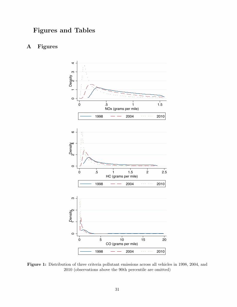
Figures and Tables

A Figures

01

23

4De

nsity

0 .5 1 1.5NOx (grams per mile)

1998 2004 2010

02

46

Dens

ity

0 .5 1 1.5 2 2.5HC (grams per mile)

1998 2004 2010

01

23

Dens

ity

0 5 10 15 20CO (grams per mile)

1998 2004 2010

Figure 1: Distribution of three criteria pollutant emissions across all vehicles in 1998, 2004, and2010 (observations above the 90th percentile are omitted)

31

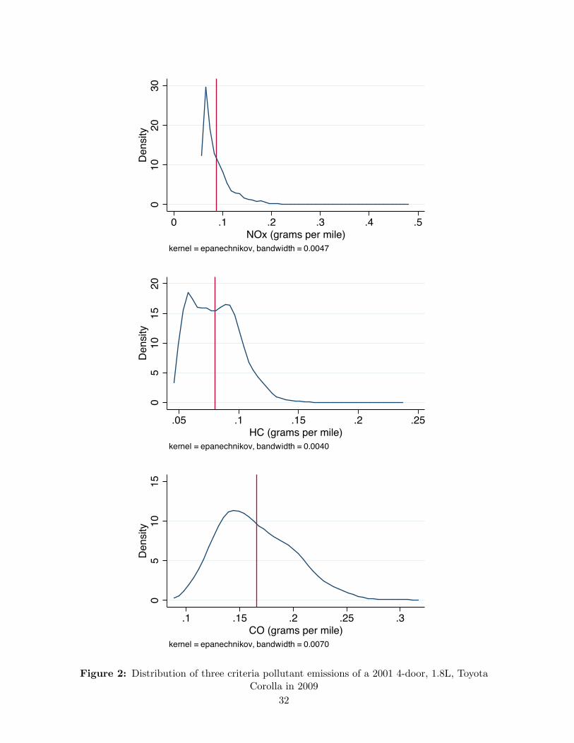
010

2030

Dens

ity

0 .1 .2 .3 .4 .5NOx (grams per mile)

kernel = epanechnikov, bandwidth = 0.0047

05

1015

20De

nsity

.05 .1 .15 .2 .25HC (grams per mile)

kernel = epanechnikov, bandwidth = 0.0040

05

1015

Dens

ity

.1 .15 .2 .25 .3CO (grams per mile)

kernel = epanechnikov, bandwidth = 0.0070

Figure 2: Distribution of three criteria pollutant emissions of a 2001 4-door, 1.8L, ToyotaCorolla in 2009

32

01

23

4De

nsity

0 .5 1 1.5NOx (grams per mile)

kernel = epanechnikov, bandwidth = 0.0323

05

1015

Dens

ity

.2 .4 .6 .8 1 1.2HC (grams per mile)

kernel = epanechnikov, bandwidth = 0.0099

01

23

4De

nsity

.5 1 1.5 2 2.5CO (grams per mile)

kernel = epanechnikov, bandwidth = 0.0295

Figure 3: Distribution of three criteria pollutant emissions of a 1995 3.8L, FWD, Ford Windstarin 1999, 2001, 2005, and 2009 (observations above the 95th percentile are omitted)

33

15202530Median Miles per Day by NOx Quartile

1998

2000

2002

2004

2006

2008

2010

Year

1st q

uarti

le2n

d qu

artil

e3r

d qu

artil

e4t

h qu

artil

e

15202530Median Miles per Day by HCs Quartile

1998

2000

2002

2004

2006

2008

2010

Year

1st q

uarti

le2n

d qu

artil

e3r

d qu

artil

e4t

h qu

artil

e

1520253035Median Miles per Day by CO Quartile

1998

2000

2002

2004

2006

2008

2010

Year

1st q

uarti

le2n

d qu

artil

e3r

d qu

artil

e4t

h qu

artil

e

182022242628Median Miles per Day by MPG Quartile

1998

2000

2002

2004

2006

2008

2010

Year

1st q

uarti

le2n

d qu

artil

e3r

d qu

artil

e4t

h qu

artil

e

Fig

ure

4:C

hang

ein

VM

Tov

ersa

mpl

eby

pollu

tant

quar

tile

34

.8.85.9.951Change in the log VMT by NOx Quartile

1998

2000

2002

2004

2006

2008

2010

Year

1st q

uarti

le2n

d qu

artil

e3r

d qu

artil

e4t

h qu

artil

e

.8.85.9.951Change in the log VMT by HCs Quartile

1998

2000

2002

2004

2006

2008

2010

Year

1st q

uarti

le2n

d qu

artil

e3r

d qu

artil

e4t

h qu

artil

e

.8.911.1Change in the log VMT by CO Quartile

1998

2000

2002

2004

2006

2008

2010

Year

1st q

uarti

le2n

d qu

artil

e3r

d qu

artil

e4t

h qu

artil

e

.9.92.94.96.981Change in the log VMT by MPG Quartile

1998

2000

2002

2004

2006

2008

2010

Year

1st q

uarti

le2n

d qu

artil

e3r

d qu

artil

e4t

h qu

artil

e

Fig

ure

5:C

hang

ein

the

log

ofV

MT

over

sam

ple

bypo

lluta

ntqu

arti

le

35

−1

−.8

−.6

−.4

−.2

0E

last

icity

0 5 10 15 20 25Age of Vehicle

Cars Trucks

Elasticity of VMT With Respect to the Price of Gasoline

Figure 6: Elasticity by vehicles’ vintage

−1

−.8

−.6

−.4

−.2

0.2

Ela

stic

ity

0 20 40 60 80 100Percentile

HC NO CO MPG Weight

Elasticity of VMT With Respect to the Price of Gasoline

Figure 7: Non-parametric relationships between elasticity and externality

36

−1

−.8

−.6

−.4

−.2

0.2

Ela

stic

ity

0 20 40 60 80 100Percentile

Unsmoothed

−1

−.8

−.6

−.4

−.2

0.2

Ela

stic

ity

0 20 40 60 80 100Percentile

LOWESS With Subsets of N*.05

−1

−.8

−.6

−.4

−.2

0.2

Ela

stic

ity

0 20 40 60 80 100Percentile

LOWESS With Subsets of N*.16

−1

−.8

−.6

−.4

−.2

0.2

Ela

stic

ity

0 20 40 60 80 100Percentile

LOWESS With Subsets of N*.27

−1

−.8

−.6

−.4

−.2

0.2

Ela

stic

ity

0 20 40 60 80 100Percentile

LOWESS With Subsets of N*.38

−1

−.8

−.6

−.4

−.2

0.2

Ela

stic

ity

0 20 40 60 80 100Percentile

LOWESS With Subsets of N*.49

Elasticity of VMT over Centiles of g/mile HC

Figure 8: The effect of bandwidth on the non-parameteric function

37

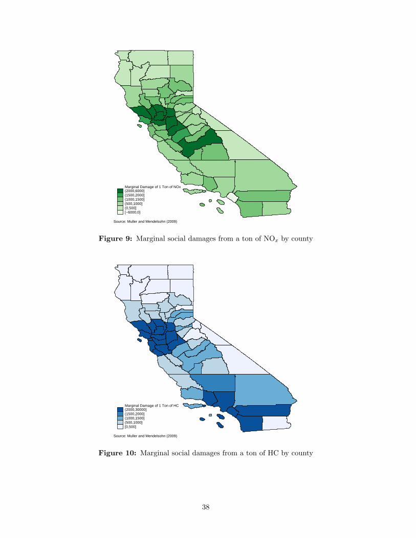
Marginal Damage of 1 Ton of NOx(2000,6000](1500,2000](1000,1500](500,1000](0,500][−6000,0]

Source: Muller and Mendelsohn (2009)

Figure 9: Marginal social damages from a ton of NOx by county

Marginal Damage of 1 Ton of HC(2000,30000](1500,2000](1000,1500](500,1000][0,500]

Source: Muller and Mendelsohn (2009)

Figure 10: Marginal social damages from a ton of HC by county

38

Negative Elasticity of VMT to Gasoline Prices(.32,.4](.24,.32](.16,.24](.08,.16][0,.08]Change of Ownership County

Source: Authors’ Calculations

Figure 11: Estimated VMT elasticty by county

Cobenefits per Ton Carbon(60,150](40,60](30,40](20,30](10,20][0,10]Change of Ownership County

Source: Authors’ Calculations

Figure 12: Estimated co-benefits by county

39

Butte

Contra Costa

El Dorado

FresnoKern

Kings

Los Angeles

MaderaMercedNapa

Orange

Placer

San Benito

San DiegoSan Joaquin

San Mateo

Shasta

Solano

Sonoma

Stanislaus

Tehama

050

100

150

Co-B

enefi

ts fr

om G

as T

ax (p

er to

n of

CO

2)

10 12 14 16Log of Population

Figure 13: Estimated county-level co-benefits verse the log of county population

Ozone formation in urban smogOzone formation in urban smog! Daytime ozone forms via different paths, examples are from

Carbon Monoxide

Methane

Formaldehyde

Ethane

or Acetaldehyde

! (Lower) limiting factors

are the amounts of NOx

and VOC in the air.

! One (nighttime) reaction removing ozone from the atmosphere is:

NO2. + O3 ! NO3

. + O2

The NO3 radical further reacts to N2O5 and HNO3

Figure 14: Level-sets of smog formation. Taken fromhttp://voh.chem.ucla.edu/vohtar/spring06/classes/103/pdf/Lect501.pdf.

40

0.0

00

1.0

00

2.0

00

3D

en

sity

0 10000 20000 30000 40000 50000Damage from HCs ($/ton)

California Rest of the US

0.0

00

2.0

00

4.0

00

6.0

00

8D

en

sity

-5000 0 5000 10000 15000Damage from NOx ($/ton)

California Rest of the US

0.0

00

05.

00

01.0

00

15.0

00

2D

en

sity

0 20000 40000 60000Sum of Damages from NOx and HCs ($/ton)

California Rest of the US

Figure 15: Distributions of marginal damages from Muller and Mendelsohn (2009) for Californiaand the rest of the US

41

01

02

03

0D

en

sity

.2 .4 .6 .8HCs/mile

California Rest of the US

02

46

81

0D

en

sity

1 1.2 1.4 1.6 1.8 2 2.2NOx/mile

California Rest of the US

0.5

11

.5D

en

sity

5 7 9 11 13 15CO/mile

California Rest of the US

Figure 16: Distributions of per-mile emissions for California and the rest of the US

42

0200400600Density

0.0

05

.01

Da

ma

ge

fro

m H

Cs (

$/m

ile

)

Ca

lifo

rnia

Re

st o

f th

e U

S

0200400600800Density

0.0

05

.01

.01

5D

am

ag

e fro

m N

Ox (

$/m

ile

)

Ca

lifo

rnia

Re

st o

f th

e U

S

050010001500Density

.00

5.0

07

5.0

1.0

12

5D

am

ag

e fro

m C

O (

$/m

ile

)

Ca

lifo

rnia

Re

st o

f th

e U

S

0100200300Density

.00

2.0

04

.00

6.0

08

.01

.01

2D

am

ag

e fro

m H

Cs, N

Ox, a

nd

CO

($

/mile

)

Ca

lifo

rnia

Re

st o

f th

e U

S

Fig

ure

17:

Dis

trib

utio

nsof

per-

mile

dam

ages

for

Cal

iforn

iaan

dth

ere

stof

the

US

43

B Tables

Table 1: Summary Statistics

Vehicle Age Year

All 4-9 10-15 16-28 1998 2008

Weighted Fuel Economy 23.49 23.29 23.67 23.67 24.09 23.04(5.300) (5.224) (5.319) (5.477) (5.402) (5.157)

Average $/mile 0.0893 0.0843 0.0902 0.103 0.0581 0.128(0.0394) (0.0369) (0.0400) (0.0420) (0.0133) (0.0306)

Odometer (00000s) 1.188 0.923 1.362 1.607 1.022 1.292(0.594) (0.448) (0.564) (0.684) (0.521) (0.606)

Grams/mile HC 0.749 0.226 0.762 2.049 1.412 0.510(1.180) (0.281) (1.064) (1.712) (1.524) (0.973)

Grams/mile CO 5.269 0.521 4.915 18.47 12.27 3.136(12.84) (1.664) (11.07) (21.25) (18.95) (10.26)

Grams/mile NOx 0.664 0.328 0.751 1.321 1.060 0.498(0.638) (0.309) (0.608) (0.740) (0.921) (0.537)

Failed Smog Check 0.0947 0.0455 0.117 0.202 0.0557 0.107(0.293) (0.208) (0.321) (0.401) (0.229) (0.309)

Average HH Income 48277.8 49998.8 47279.1 45188.5 50228.4 48044.1(17108.2) (17702.9) (16633.2) (15628.0) (18067.0) (16887.5)

Truck 0.386 0.403 0.367 0.375 0.331 0.426(0.487) (0.491) (0.482) (0.484) (0.471) (0.494)

Vehicle Age 10.39 6.644 12.08 18.45 8.975 11.49(4.477) (1.615) (1.682) (2.424) (3.448) (4.741)

N 7015260 3333774 2699413 981234 386753 541246Statistics are means with standard deviations presented below in parentheses. Weighted fuel economy is from

EPA. Dollars per mile is the average gasoline price from EIA in between Smog Checks divided by fuel economy.

Average household income is taken from the 2000 Census ZCTA where the Smog Check occurred. Dataset

contains one observation per vehicle per year in which a Smog Check occurred.

44

Tab

le2:

Ave

rage

Pol

luta

ntR

ates

Per

Mile

Tra

vele

dby

Yea

r

Nit

roge

nO

xide

sH

ydro

carb

ons

Car

bon

Mon

oxid

eG

asol

ine

Yea

rM

ean

SDM

ean

CV

Mea

nSD

Mea

nC

VM

ean

SDM

ean

CV

Mea

nSD

1998

1.16

11.

051

0.53

61.

662

1.86

60.

504

15.4

0024

.739

0.51

60.

043

0.01

019

991.

187

0.98

30.

455

1.66

51.

864

0.46

415

.227

24.9

520.

485

0.04

30.

010

2000

1.09

40.

915

0.44

11.

535

1.82

60.

460

13.5

3923

.849

0.47

60.

044

0.01

020

010.

982

0.85

70.

427

1.35

41.

769

0.46

411

.689

23.1

230.

461

0.04

40.

010

2002

0.87

60.

816

0.41

81.

145

1.67

90.

446

9.69

421

.381

0.43

00.

044

0.01

020

030.

791

0.78

00.

401

0.99

71.

563

0.43

27.

940

19.5

030.

395

0.04

50.

010

2004

0.71

50.

742

0.38

00.

855

1.46

90.

421

6.56

117

.581

0.36

30.

045

0.01

020

050.

735

0.71

30.

393

0.85

21.

444

0.45

56.

375

17.5

190.

379

0.04

50.

010

2006

0.63

80.

667

0.38

20.

718

1.35

10.

430

5.15

715

.887

0.35

00.

045

0.01

020

070.

572

0.63

40.

377

0.62

81.

261

0.43

14.

308

14.5

090.

334

0.04

50.

010

2008

0.51

20.

602

0.37

30.

545

1.18

50.

400

3.55

613

.064

0.31

70.

046

0.01

020

090.

478

0.59

00.

379

0.49

61.

148

0.41

23.

120

12.1

470.

316

0.04

60.

011

2010

0.46

20.

566

0.40

20.

460

1.00

20.

427

2.74

110

.901

0.32

30.

046

0.01

0

N10

4323

7410

4323

7410

6663

4813

3977

95N

ote

:M

ean

CV

isth

eav

erage

VIN

Pre

fix-l

evel

coeffi

cien

tof

vari

ati

on

(SD

/M

ean).

Gaso

line

ism

easu

red

ingallons

per

mile,

while

the

rem

ain

ing

polluta

nt

rate

sare

mea

sure

din

gra

ms

per

mile.

45

Table 3: Vehicle Miles Traveled, Dollars Per Mile, and Nitrogen Oxides (Quartiles by year)

(1) (2) (3) (4) (5) (6) (7)Model 1 Model 2 Model 3 Model 4 Model 5 Model 6 Model7

ln(DPM) -0.399** -0.140** -0.224** -0.257** -0.078(0.068) (0.040) (0.052) (0.055) (0.068)

ln(DPM) * NO Q1 -0.102** -0.094(0.015) (0.073)

ln(DPM) * NO Q2 -0.144** -0.183**(0.014) (0.067)

ln(DPM) * NO Q3 -0.175** -0.246**(0.014) (0.066)

ln(DPM) * NO Q4 -0.204** -0.323**(0.014) (0.069)

ln(DPM)*NO Centile -0.003**(0.000)

NO Q2 0.212** 0.226**(0.014) (0.023)

NO Q3 0.409** 0.408**(0.019) (0.038)

NO Q4 0.630** 0.636**(0.022) (0.043)

NO Centile 0.008**(0.001)

Truck 0.125** 0.097* 0.073** 0.038(0.042) (0.048) (0.010) (0.075)

Year Fixed Effects Yes Yes Yes Yes Yes Yes YesWithin-Year Time Trends Yes Yes Yes Yes Yes Yes YesVintage Fixed Effects Yes Yes Yes Yes Yes Yes YesDemographics Yes Yes Yes Yes Yes Yes YesMake Fixed Effects No Yes Yes No No No NoVin Prefix Fixed Effects No No No Yes No No NoVehicle Fixed Effects No No No No Yes Yes Yes

Observations 3640436 3640436 2904026 3640436 3640436 2904026 2904026R-squared 0.141 0.159 0.172 0.083 0.110 0.105 0.106

46

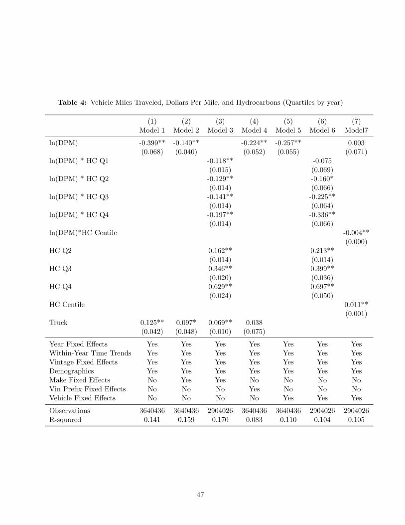
Table 4: Vehicle Miles Traveled, Dollars Per Mile, and Hydrocarbons (Quartiles by year)

(1) (2) (3) (4) (5) (6) (7)Model 1 Model 2 Model 3 Model 4 Model 5 Model 6 Model7

ln(DPM) -0.399** -0.140** -0.224** -0.257** 0.003(0.068) (0.040) (0.052) (0.055) (0.071)

ln(DPM) * HC Q1 -0.118** -0.075(0.015) (0.069)

ln(DPM) * HC Q2 -0.129** -0.160*(0.014) (0.066)

ln(DPM) * HC Q3 -0.141** -0.225**(0.014) (0.064)

ln(DPM) * HC Q4 -0.197** -0.336**(0.014) (0.066)

ln(DPM)*HC Centile -0.004**(0.000)

HC Q2 0.162** 0.213**(0.014) (0.014)

HC Q3 0.346** 0.399**(0.020) (0.036)

HC Q4 0.629** 0.697**(0.024) (0.050)

HC Centile 0.011**(0.001)

Truck 0.125** 0.097* 0.069** 0.038(0.042) (0.048) (0.010) (0.075)

Year Fixed Effects Yes Yes Yes Yes Yes Yes YesWithin-Year Time Trends Yes Yes Yes Yes Yes Yes YesVintage Fixed Effects Yes Yes Yes Yes Yes Yes YesDemographics Yes Yes Yes Yes Yes Yes YesMake Fixed Effects No Yes Yes No No No NoVin Prefix Fixed Effects No No No Yes No No NoVehicle Fixed Effects No No No No Yes Yes Yes

Observations 3640436 3640436 2904026 3640436 3640436 2904026 2904026R-squared 0.141 0.159 0.170 0.083 0.110 0.104 0.105

47

Table 5: Vehicle Miles Traveled, Dollars Per Mile, and Carbon Monoxide (Quartiles by year)

(1) (2) (3) (4) (5) (6) (7)Model 1 Model 2 Model 3 Model 4 Model 5 Model 6 Model7

ln(DPM) -0.399** -0.140** -0.224** -0.257** -0.008(0.068) (0.040) (0.052) (0.055) (0.069)

ln(DPM) * CO Q1 -0.046** -0.071(0.015) (0.067)

ln(DPM) * CO Q2 -0.072** -0.168*(0.014) (0.064)

ln(DPM) * CO Q3 -0.097** -0.237**(0.014) (0.061)

ln(DPM) * CO Q4 -0.129** -0.333**(0.015) (0.066)

ln(DPM)*CO Centile -0.004**(0.000)

CO Q2 0.196** 0.239**(0.015) (0.015)

CO Q3 0.420** 0.440**(0.021) (0.035)

CO Q4 0.664** 0.723**(0.025) (0.060)

CO Centile 0.012**(0.001)

Truck 0.125** 0.097* 0.045** 0.038(0.042) (0.048) (0.010) (0.075)

Year Fixed Effects Yes Yes Yes Yes Yes Yes YesWithin-Year Time Trends Yes Yes Yes Yes Yes Yes YesVintage Fixed Effects Yes Yes Yes Yes Yes Yes YesDemographics Yes Yes Yes Yes Yes Yes YesMake Fixed Effects No Yes Yes No No No NoVin Prefix Fixed Effects No No No Yes No No NoVehicle Fixed Effects No No No No Yes Yes Yes

Observations 3640436 3640436 2965945 3640436 3640436 2965945 2965945R-squared 0.141 0.159 0.169 0.083 0.110 0.104 0.105

48

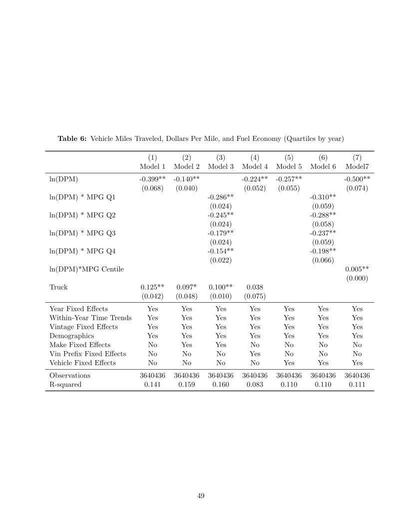
Table 6: Vehicle Miles Traveled, Dollars Per Mile, and Fuel Economy (Quartiles by year)

(1) (2) (3) (4) (5) (6) (7)Model 1 Model 2 Model 3 Model 4 Model 5 Model 6 Model7

ln(DPM) -0.399** -0.140** -0.224** -0.257** -0.500**(0.068) (0.040) (0.052) (0.055) (0.074)

ln(DPM) * MPG Q1 -0.286** -0.310**(0.024) (0.059)

ln(DPM) * MPG Q2 -0.245** -0.288**(0.024) (0.058)

ln(DPM) * MPG Q3 -0.179** -0.237**(0.024) (0.059)

ln(DPM) * MPG Q4 -0.154** -0.198**(0.022) (0.066)

ln(DPM)*MPG Centile 0.005**(0.000)

Truck 0.125** 0.097* 0.100** 0.038(0.042) (0.048) (0.010) (0.075)

Year Fixed Effects Yes Yes Yes Yes Yes Yes YesWithin-Year Time Trends Yes Yes Yes Yes Yes Yes YesVintage Fixed Effects Yes Yes Yes Yes Yes Yes YesDemographics Yes Yes Yes Yes Yes Yes YesMake Fixed Effects No Yes Yes No No No NoVin Prefix Fixed Effects No No No Yes No No NoVehicle Fixed Effects No No No No Yes Yes Yes

Observations 3640436 3640436 3640436 3640436 3640436 3640436 3640436R-squared 0.141 0.159 0.160 0.083 0.110 0.110 0.111

49

Table 7: Vehicle Miles Traveled, Dollars Per Mile, and Weight (Quartiles by year)

(1) (2) (3) (4) (5) (6) (7)Model 1 Model 2 Model 3 Model 4 Model 5 Model 6 Model7

ln(DPM) -0.399** -0.140** -0.224** -0.257** -0.157**(0.068) (0.040) (0.052) (0.055) (0.058)

ln(DPM) * Weight Q1 -0.188** -0.226**(0.018) (0.056)

ln(DPM) * Weight Q2 -0.159** -0.252**(0.017) (0.056)

ln(DPM) * Weight Q3 -0.191** -0.271**(0.019) (0.056)

ln(DPM) * Weight Q4 -0.222** -0.282**(0.017) (0.059)

ln(DPM)*Weight Centile -0.002**(0.000)

Truck 0.125** 0.097* 0.097** 0.038(0.042) (0.048) (0.010) (0.075)

Year Fixed Effects Yes Yes Yes Yes Yes Yes YesWithin-Year Time Trends Yes Yes Yes Yes Yes Yes YesVintage Fixed Effects Yes Yes Yes Yes Yes Yes YesDemographics Yes Yes Yes Yes Yes Yes YesMake Fixed Effects No Yes Yes No No No NoVin Prefix Fixed Effects No No No Yes No No NoVehicle Fixed Effects No No No No Yes Yes Yes

Observations 3640436 3640436 3619192 3640436 3640436 3619192 3619192R-squared 0.141 0.159 0.160 0.083 0.110 0.110 0.110

50

Table 8: Vehicle Miles Traveled, Dollars Per Mile, and Nitrogen Oxides (Quartiles by age range)

(1) (2) (3) (4) (5) (6)4-9 10-15 16-27 4-9 10-15 16-27

ln(DPM) -0.201** -0.227** -0.634**(0.073) (0.086) (0.224)

ln(DPM) * NO Q1 -0.166* -0.109 -0.531*(0.073) (0.075) (0.239)

ln(DPM) * NO Q2 -0.197* -0.181* -0.594*(0.076) (0.080) (0.240)

ln(DPM) * NO Q3 -0.215** -0.224** -0.691**(0.075) (0.080) (0.236)

ln(DPM) * NO Q4 -0.226** -0.250** -0.722**(0.075) (0.083) (0.249)

NO Q2 0.081** 0.191** 0.175**(0.022) (0.027) (0.031)

NO Q3 0.130** 0.310** 0.428**(0.023) (0.034) (0.054)

NO Q4 0.174** 0.395** 0.539**(0.032) (0.046) (0.055)

Year Fixed Effects Yes Yes Yes Yes Yes YesWithin-Year Time Trends Yes Yes Yes Yes Yes YesVintage Fixed Effects Yes Yes Yes Yes Yes YesDemographics Yes Yes Yes Yes Yes YesVin Prefix Fixed Effects No No No No No NoVehicle Fixed Effects Yes Yes Yes Yes Yes Yes

Observations 1548635 1535834 555967 1182350 1239393 482283R-squared 0.040 0.064 0.083 0.038 0.066 0.081

51

Table 9: Vehicle Miles Traveled, Dollars Per Mile, and Hydrocarbons (Quartiles by age range)

(1) (2) (3) (4) (5) (6)4-9 10-15 16-27 4-9 10-15 16-27

ln(DPM) -0.201** -0.227** -0.634**(0.073) (0.086) (0.224)

ln(DPM) * HC Q1 -0.162* -0.118 -0.467+(0.072) (0.071) (0.236)

ln(DPM) * HC Q2 -0.191* -0.183* -0.542*(0.075) (0.076) (0.236)

ln(DPM) * HC Q3 -0.192* -0.216** -0.650**(0.075) (0.078) (0.229)

ln(DPM) * HC Q4 -0.218** -0.247** -0.740**(0.073) (0.082) (0.240)

HC Q2 0.075** 0.171** 0.204**(0.019) (0.023) (0.045)

HC Q3 0.089** 0.262** 0.466**(0.020) (0.032) (0.064)

HC Q4 0.162** 0.344** 0.705**(0.023) (0.050) (0.086)

Year Fixed Effects Yes Yes Yes Yes Yes YesWithin-Year Time Trends Yes Yes Yes Yes Yes YesVintage Fixed Effects Yes Yes Yes Yes Yes YesDemographics Yes Yes Yes Yes Yes YesVin Prefix Fixed Effects No No No No No NoVehicle Fixed Effects Yes Yes Yes Yes Yes Yes

Observations 1548635 1535834 555967 1182350 1239393 482283R-squared 0.040 0.064 0.083 0.038 0.065 0.081

52

Table 10: Vehicle Miles Traveled, Dollars Per Mile, and Carbon Monoxide (Quartiles by agerange)

(1) (2) (3) (4) (5) (6)4-9 10-15 16-27 4-9 10-15 16-27

ln(DPM) -0.201** -0.227** -0.634**(0.073) (0.086) (0.224)

ln(DPM) * CO Q1 -0.162* -0.090 -0.483*(0.074) (0.071) (0.226)

ln(DPM) * CO Q2 -0.204** -0.170* -0.571*(0.073) (0.075) (0.225)

ln(DPM) * CO Q3 -0.218** -0.203* -0.662**(0.074) (0.082) (0.231)

ln(DPM) * CO Q4 -0.241** -0.237** -0.721**(0.073) (0.084) (0.236)

CO Q2 0.095** 0.209** 0.234**(0.015) (0.021) (0.045)

CO Q3 0.139** 0.302** 0.467**(0.018) (0.038) (0.078)

CO Q4 0.205** 0.410** 0.632**(0.034) (0.053) (0.104)

Year Fixed Effects Yes Yes Yes Yes Yes YesWithin-Year Time Trends Yes Yes Yes Yes Yes YesVintage Fixed Effects Yes Yes Yes Yes Yes YesDemographics Yes Yes Yes Yes Yes YesVin Prefix Fixed Effects No No No No No NoVehicle Fixed Effects Yes Yes Yes Yes Yes Yes

Observations 1548635 1535834 555967 1215664 1263957 486324R-squared 0.040 0.064 0.083 0.038 0.066 0.081

53

Table 11: Vehicle Miles Traveled, Dollars Per Mile, and Fuel Economy (Quartiles by age range)

(1) (2) (3) (4) (5) (6)4-9 10-15 16-27 4-9 10-15 16-27

ln(DPM) -0.201** -0.227** -0.634**(0.073) (0.086) (0.224)

ln(DPM) * MPG Q1 -0.217** -0.248** -0.678**(0.073) (0.088) (0.224)

ln(DPM) * MPG Q2 -0.206** -0.236** -0.667**(0.073) (0.088) (0.229)

ln(DPM) * MPG Q3 -0.195** -0.218* -0.627**(0.073) (0.084) (0.225)

ln(DPM) * MPG Q4 -0.186* -0.204* -0.570*(0.075) (0.081) (0.225)

Year Fixed Effects Yes Yes Yes Yes Yes YesWithin-Year Time Trends Yes Yes Yes Yes Yes YesVintage Fixed Effects Yes Yes Yes Yes Yes YesDemographics Yes Yes Yes Yes Yes YesVin Prefix Fixed Effects No No No No No NoVehicle Fixed Effects Yes Yes Yes Yes Yes Yes

Observations 1548635 1535834 555967 1548635 1535834 555967R-squared 0.040 0.064 0.083 0.040 0.064 0.084

54

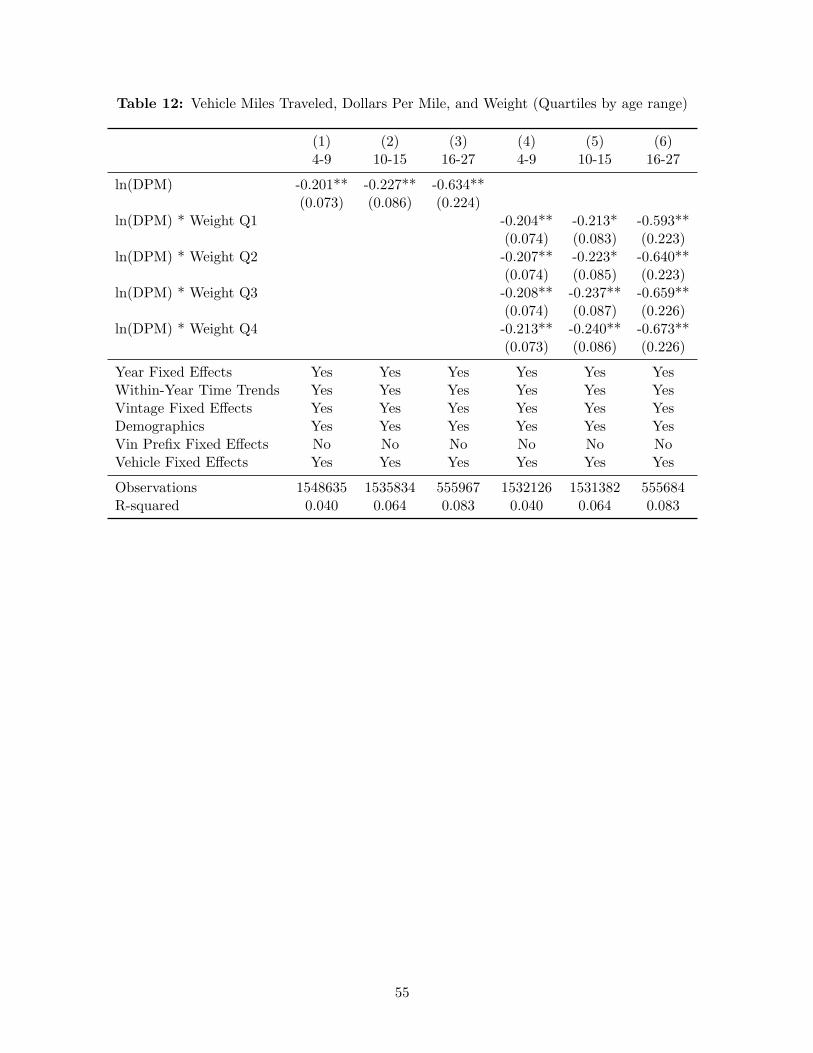
Table 12: Vehicle Miles Traveled, Dollars Per Mile, and Weight (Quartiles by age range)

(1) (2) (3) (4) (5) (6)4-9 10-15 16-27 4-9 10-15 16-27

ln(DPM) -0.201** -0.227** -0.634**(0.073) (0.086) (0.224)

ln(DPM) * Weight Q1 -0.204** -0.213* -0.593**(0.074) (0.083) (0.223)

ln(DPM) * Weight Q2 -0.207** -0.223* -0.640**(0.074) (0.085) (0.223)

ln(DPM) * Weight Q3 -0.208** -0.237** -0.659**(0.074) (0.087) (0.226)

ln(DPM) * Weight Q4 -0.213** -0.240** -0.673**(0.073) (0.086) (0.226)

Year Fixed Effects Yes Yes Yes Yes Yes YesWithin-Year Time Trends Yes Yes Yes Yes Yes YesVintage Fixed Effects Yes Yes Yes Yes Yes YesDemographics Yes Yes Yes Yes Yes YesVin Prefix Fixed Effects No No No No No NoVehicle Fixed Effects Yes Yes Yes Yes Yes Yes

Observations 1548635 1535834 555967 1532126 1531382 555684R-squared 0.040 0.064 0.083 0.040 0.064 0.083

55

Table 13: VMT Elasticity for a Sample of Households, 2000-2008

(1) (2) (3)

ln(DPM) * MPG Q1 -0.131∗∗∗ -0.132∗∗∗ -0.148∗∗∗

(0.0397) (0.0396) (0.0399)ln(DPM) * MPG Q2 -0.114∗∗ -0.116∗∗ -0.132∗∗∗

(0.0396) (0.0396) (0.0399)ln(DPM) * MPG Q3 -0.0749 -0.0796∗ -0.0952∗

(0.0396) (0.0396) (0.0399)ln(DPM) * MPG Q4 -0.0339 -0.0405 -0.0559

(0.0398) (0.0398) (0.0400)ln(DPM) * Higher MPG in HH -0.0274∗∗∗ -0.0284∗∗∗

(0.00423) (0.00423)Dollars per Mile * Lower MPG in HH 0.0503∗∗∗ 0.0499∗∗∗

(0.00433) (0.00433)Higher MPG in HH 0.0552∗∗∗ 0.0573∗∗∗

(0.00945) (0.00945)Lower MPG in HH -0.112∗∗∗ -0.111∗∗∗

(0.00867) (0.00866)ln(DPM) * HH Income Q2 -0.00183

(0.00473)ln(DPM) * HH Income Q3 0.0211∗∗∗

(0.00492)ln(DPM) * HH Income Q4 0.0322∗∗∗

(0.00533)

Year Fixed Effects Yes Yes YesWithin-Year Time Trends Yes Yes YesVintage Fixed Effects Yes Yes YesDemographics Yes Yes YesVehicle Fixed Effects Yes Yes Yes

Observations 7549359 7549359 7549359R-squared 0.106 0.106 0.106Standard errors in parentheses∗ p < 0.05, ∗∗ p < 0.01, ∗∗∗ p < 0.001

56

Table 14: VMT Elasticity by Income Quartile, 2000-2008

40% Sample of HHs 10% Sample of VINs

ln(DPM) * HH Income Q1 -0.104∗∗ -0.303∗∗∗

(0.0398) (0.0696)ln(DPM) * HH Income Q2 -0.106∗∗ -0.300∗∗∗

(0.0396) (0.0695)ln(DPM) * HH Income Q3 -0.0841∗ -0.297∗∗∗

(0.0396) (0.0697)ln(DPM) * HH Income Q4 -0.0753 -0.274∗∗∗

(0.0396) (0.0695)

Year Fixed Effects Yes YesWithin-Year Time Trends Yes YesVintage Fixed Effects Yes YesDemographics Yes YesVehicle Fixed Effects Yes Yes

Observations 7549359 2489375R-squared 0.105 0.088Standard errors in parentheses∗ p < 0.05, ∗∗ p < 0.01, ∗∗∗ p < 0.001

57

Table 15: Hazard of Scrappage: Cox Proportional Hazard Model

Model 1 Model 2 Model 3 Model 4 Model 5

Dollars per Mile 0.918+ 0.957(0.045) (0.036)

DPM * Failed Smog Check 1.099** 1.069* 1.058* 1.038+(0.033) (0.028) (0.026) (0.023)

Failed Last Smog Check 7.551** 7.993** 8.735** 9.379**(0.264) (0.271) (0.231) (0.234)

DPM * NO Quartile 1 0.800** 0.922(0.050) (0.049)

DPM * NO Quartile 2 0.841** 0.925(0.046) (0.045)

DPM * NO Quartile 3 0.863** 0.956(0.038) (0.030)

DPM * NO Quartile 4 0.924* 0.980(0.037) (0.022)

Vehicle Ages 10-15

DPM * NO Quartile 1 0.815+(0.087)

DPM * NO Quartile 2 0.790*(0.086)

DPM * NO Quartile 3 0.800*(0.081)

DPM * NO Quartile 4 0.765**(0.073)

Failed Smog Check 7.460**(0.677)

DPM * Failed Smog Check 1.124*(0.061)

Vehicle Ages 16+

DPM * NO Quartile 1 1.087**(0.028)

DPM * NO Quartile 2 1.063*(0.028)

DPM * NO Quartile 3 1.073*(0.035)

DPM * NO Quartile 4 1.062+(0.038)

Failed Smog Check 10.862**(0.548)

DPM * Failed Smog Check 0.992(0.022)

Station ZIP Code Characteristics Yes Yes Yes Yes YesQuadratic Time Trend in Days Yes Yes Yes Yes YesVehicle Characteristics Yes Yes Yes Yes YesQuartiles of NO No Yes No Yes YesStratified on Vin Prefix No No Yes Yes YesObservations 3176325 2623649 3176325 2623649 2623649

Note: Coefficients on dollars per mile scaled for a 5-cent change

58

Table 16: Hazard of Scrappage: Cox Proportional Hazard Model

Model 1 Model 2 Model 3 Model 4 Model 5

Dollars per Mile 0.918+ 0.957(0.045) (0.036)

DPM * Failed Smog Check 1.099** 1.072+ 1.058* 1.096**(0.033) (0.038) (0.026) (0.028)

Failed Last Smog Check 7.551** 7.778** 8.735** 8.210**(0.264) (0.293) (0.231) (0.229)

DPM * MPG Quartile 1 0.985 0.828**(0.058) (0.050)

DPM * MPG Quartile 2 1.002 0.924(0.063) (0.048)

DPM * MPG Quartile 3 0.997 1.014(0.072) (0.074)

DPM * MPG Quartile 4 1.067 1.173*(0.090) (0.082)

Vehicle Ages 10-15

DPM * MPG Quartile 1 0.740**(0.071)

DPM * MPG Quartile 2 0.746**(0.081)

DPM * MPG Quartile 3 0.862(0.111)

DPM * MPG Quartile 4 0.944(0.181)

Failed Smog Check 6.780**(0.504)

DPM * Failed Smog Check 1.161**(0.057)

Vehicle Ages 16+

DPM * MPG Quartile 1 0.989(0.034)

DPM * MPG Quartile 2 1.086*(0.036)

DPM * MPG Quartile 3 1.132*(0.061)

DPM * MPG Quartile 4 1.063(0.040)

Failed Smog Check 10.075**(0.469)

DPM * Failed Smog Check 1.019(0.022)

Station ZIP Code Characteristics Yes Yes Yes Yes YesQuadratic Time Trend in Days Yes Yes Yes Yes YesVehicle Characteristics Yes Yes Yes Yes YesStratified on Vin Prefix No No Yes Yes YesObservations 3176325 3176325 3176325 3176325 3176325

Note: Coefficients on dollars per mile scaled for a 5-cent change

59

Tab

le17

:C

oben

efits

ofa

Gas

olin

eT

ax,

No

Het

erog

enei

ty

∆C

onsu

mpt

ion

∆C

O2

DW

LC

rite

ria

Ben

efit

Net

Cos

t

(Gal

lons

)(T

ons)

($)

(NO

x$)

(HC

$)(C

O$)

(Tot

al$)

(%D

WL

)(P

erC

O2)

(Per

CO

2)

1998

798.

27.

662

548.

03.

262

227.

492

.86

322.

513

4.9

96.4

6-2

4.94

1999

807.

87.

755

538.

95.

291

254.

299

.82

358.

612

4.5

86.5

4-1

7.05

2000

835.

88.

023

537.

45.

791

250.

993

.12

349.

411

4.9

76.9

7-9

.982

2001

773.

27.

422

478.

35.

449

189.

868

.68

263.

698

.67

63.5

80.

859

2002

735.

87.

064

444.

48.

176

229.

080

.83

317.

680

.92

50.9

112

.00

2003

780.

37.

491

460.

68.

733

195.

767

.37

271.

568

.28

41.9

919

.50

2004

821.

17.

883

472.

410

.18

159.

855

.34

225.

053

.77

32.2

227

.70

2005

767.

67.

369

425.

98.

478

113.

838

.01

160.

043

.21

24.9

732

.82

2006

637.

26.

117

340.

36.

740

85.0

427

.30

118.

940

.48

22.5

233

.11

2007

677.

46.

503

350.

25.

957

63.0

219

.08

87.9

029

.19

15.7

238

.13

2008

604.

15.

799

302.

04.

419

48.8

213

.75

66.8

526

.55

13.8

338

.26

Ave

rage

748.

97.

190

445.

36.

589

165.

259

.65

231.

174

.13

47.7

913

.67

Note

:A

llunit

sare

inm

illions.

Dollar

figure

sare

inflati

on

adju

sted

to2008

term

s.N

Ox

and

HC

are

valu

edas

inM

uller

and

Men

del

sohn’s

(2009)

USE

PA

scen

ari

oby

the

county

wher

eea

chveh

icle

rece

ived

its

Sm

og

Chec

k.

The

valu

esva

rysu

bst

anti

ally

acr

oss

counti

es,

but

ap

opula

tion-w

eighte

d

aver

age

for

the

state

valu

esH

Cat

$10109.8

1p

erto

np

eryea

r,and

NO

xat

$826.3

4p

erto

np

eryea

r.C

Ois

valu

edat

$802.8

8,

as

per

the

med

ian

valu

eof

Matt

hew

sand

Lav

e(2

000).

60

Tab

le18

:C

oben

efits

ofa

Gas

olin

eT

ax,

Tak

ing

Het

erog

enei

tyin

toA

ccou

nt(N

oE

xten

sive

Mar

gin

Effe

ct)

∆C

onsu

mpt

ion

∆C

O2

DW

LC

rite

ria

Ben

efit

Net

Cos

t

(Gal

lons

)(T

ons)

($)

(NO

x$)

(HC

$)(C

O$)

(Tot

al$)

(%D

WL

)(P

erC

O2)

(Per

CO

2)

1998

520.

74.

999

357.

57.

214

506.

522

2.5

733.

820

7.6

148.

5-7

6.94

1999

505.

44.

852

337.

18.

575

444.

919

0.5

642.

819

1.5

133.

1-6

3.59

2000

522.

95.

020

336.

38.

343

431.

617

8.0

617.

218

8.7

126.

4-5

9.44

2001

485.

74.

662

300.

48.

574

344.

414

2.2

494.

716

5.4

106.

6-4

2.12

2002

381.

33.

661

230.

37.

055

235.

094

.66

336.

414

6.5

92.1

7-2

9.26

2003

373.

33.

584

220.

47.

398

199.

878

.60

285.

513

0.0

79.9

3-1

8.43

2004

371.

43.

565

213.

68.

732

158.

863

.44

230.

710

8.4

64.9

5-5

.032

2005

294.

42.

826

163.

36.

970

110.

843

.22

160.

898

.90

57.1

60.

634

2006

259.

82.

494

138.

75.

697

85.7

932

.54

123.

989

.80

49.9

55.

675

2007

221.

32.

124

114.

44.

529

64.6

524

.21

93.2

782

.06

44.1

99.

661

2008

208.

52.

001

104.

23.

870

52.7

019

.17

75.6

372

.94

37.9

914

.09

Ave

rage

376.

83.

617

228.

86.

996

239.

599

.00

345.

013

4.7

85.5

3-2

4.07

Note

:A

llunit

sare

inm

illions.

Dollar

figure

sare

inflati

on

adju

sted

to2008

term

s.N

Ox

and

HC

are

valu

edas

inM

uller

and

Men

del

sohn’s

(2009)

USE

PA

scen

ari

oby

the

county

wher

eea

chveh

icle

rece

ived

its

Sm

og

Chec

k.

The

valu

esva

rysu

bst

anti

ally

acr

oss

counti

es,

but

ap

opula

tion-w

eighte

d

aver

age

for

the

state

valu

esH

Cat

$10109.8

1p

erto

np

eryea

r,and

NO

xat

$826.3

4p

erto

np

eryea

r.C

Ois

valu

edat

$802.8

8,

as

per

the

med

ian

valu

eof

Matt

hew

sand

Lav

e(2

000).

61

Tab

le19

:C

oben

efits

ofa

Gas

olin

eT

ax,

Tak

ing

Het

erog

enei

tyin

toA

ccou

nt

∆C

onsu

mpt

ion

∆C

O2

DW

LC

rite

ria

Ben

efit

Net

Cos

t

(Gal

lons

)(T

ons)

($)

(NO

x$)

(HC

$)(C

O$)

(Tot

al$)

(%D

WL

)(P

erC

O2)

(Per

CO

2)

1998

520.

74.

999

357.

57.

214

506.

522

2.5

733.

820

7.6

148.

5-7

6.94

1999

524.

75.

037

350.

09.

202

444.

619

0.3

643.

018

4.5

128.

2-5

8.70

2000

546.

85.

250

351.

68.

330

432.

217

8.1

617.

818

9.8

127.

1-6

0.15

2001

563.

75.

412

348.

79.

014

351.

314

3.8

503.

814

5.0

93.4

5-2

9.01

2002

472.

74.

538

285.

57.

613

252.

310

0.6

360.

212

6.5

79.6

2-1

6.70

2003

511.

74.

912

302.

18.

339

224.

387

.17

319.

510

6.1

65.2

8-3

.781

2004

563.

45.

409

324.

19.

835

187.

274

.06

270.

883

.87

50.2

69.

664

2005

489.

64.

701

271.

78.

430

139.

755

.22

203.

175

.10

43.4

014

.39

2006

434.

34.

170

231.

97.

402

116.

545

.90

169.

673

.58

40.9

314

.70

2007

463.

34.

448

239.

56.

681

97.7

838

.21

142.

559

.86

32.2

421

.61

2008

457.

84.

395

228.

95.

893

86.7

733

.46

125.

955

.33

28.8

223

.27

Ave

rage

504.

44.

843

299.

27.

996

258.

110

6.3

371.

811

8.8

76.1

6-1

4.70

Note

:A

llunit

sare

inm

illions.

Dollar

figure

sare

inflati

on

adju

sted

to2008

term

s.N

Ox

and

HC

are

valu

edas

inM

uller

and

Men

del

sohn’s

(2009)

USE

PA

scen

ari

oby

the

county

wher

eea

chveh

icle

rece

ived

its

Sm

og

Chec

k.

The

valu

esva

rysu

bst

anti

ally

acr

oss

counti

es,

but

ap

opula

tion-w

eighte

d

aver

age

for

the

state

valu

esH

Cat

$10109.8

1p

erto

np

eryea

r,and

NO

xat

$826.3

4p

erto

np

eryea

r.C

Ois

valu

edat

$802.8

8,

as

per

the

med

ian

valu

eof

Matt

hew

sand

Lav

e(2

000).

62

Table 20: Percentage Difference Between California and the rest of the US

25th Percentile Median 75th Percentile Mean

NOx g/mi -0.230 -0.291 -0.338 -0.282

NOx Damage/ton (MM) -0.439 -0.525 -0.558 -0.685

NOx Damage/mi -0.595 -0.657 -0.712 -0.761

HC g/mi -0.262 -0.321 -0.410 -0.354

HC Damage/ton 1.475 2.558 5.318 1.821

HC Damage/mi 0.602 1.134 3.358 1.035

CO g/mi -0.226 -0.321 -0.366 -0.320

CO Damage/mi -0.226 -0.321 -0.366 -0.320

NOx + HC Damage/ton (MM) 0.0191 0.994 2.337 0.787

NOx + HC + CO Damage/mi -0.353 -0.299 -0.0883 -0.295

Notes: The table reports the coefficient on the California dummy divided by the constant.

All differences are statistically significant at the 0.001 level, except for NOx g/mi and

HC Damage/mi at the 25th percentile (significant at the 0.05 level), and NOx Damage/mi.

63