the hawai`i-pacific islands cooperative ecosystems studies ...€¦ · pacific cooperative studies...
TRANSCRIPT

The Hawai`i-Pacific Islands Cooperative Ecosystems Studies Unit &
Pacific Cooperative Studies Unit UNIVERSITY OF HAWAI`I AT MĀNOA
Dr. David C. Duffy, Unit Leader Department of Botany
3190 Maile Way, St. John #408 Honolulu, Hawai’i 96822
Technical Report 188
Predicting impacts of sea level rise for cultural and natural resources in five National Park units on the Island of Hawai‘i
June 2014
Lisa Marrack1 and Patrick O’Grady1
1 University of California, Berkeley Department of Environmental Science, Policy & Management

PCSU is a cooperative program between the University of Hawai`i and U.S. National Park Service, Cooperative Ecological Studies Unit. Organization Contact Information: Lisa Marrack [email protected] Recommended Citation: Marrack, L. and P. O’Grady. 2014. Predicting impacts of sea level rise for cultural and natural resources in five National Park units on the Island of Hawai‘i.Technical Report No. 188. Pacific Cooperative Studies Unit, University of Hawai‘i, Honolulu, Hawai‘i. 40 pp. Key words: Climate change, sea level rise, Geographic Information Systems, anchialine pool, LiDAR
Place key words: Hawai‘i, Kaloko Honokohau National Historical Park, Pu‘ukohola Heiau National Historical Site, Pu‘uhonua O Honaunau National Historical Park, and Hawai‘i Volcanoes National Park, Ala Kahakai National Historic Trail Editor: David C. Duffy, PCSU Unit Leader (Email: [email protected]) Series Editor: Clifford W. Morden, PCSU Deputy Director (Email: [email protected]) About this technical report series: This technical report series began in 1973 with the formation of the Cooperative National Park Resources Studies Unit at the University of Hawai'i at Mānoa. In 2000, it continued under the Pacific Cooperative Studies Unit (PCSU). The series currently is supported by the PCSU and the Hawai'i-Pacific Islands Cooperative Ecosystem Studies Unit (HPI CESU). The Pacific Cooperative Studies Unit at the University of Hawai'i at Mānoa works to protect cultural and natural biodiversity in the Pacific while encouraging a sustainable economy. PCSU works cooperatively with private, state and federal land management organizations, allowing them to pool and coordinate their efforts to address problems across the landscape. The Hawaii-Pacific Islands Cooperative Ecosystem Studies Unit is a coalition of governmental agencies, non-governmental organizations and universities that promotes research, education and technical assistance to support better stewardship of imperiled natural and cultural resources within the Pacific.
The HPI CESU is one of 17 cooperative ecosystem studies units across the U.S.

2
Table of Contents
LIST of FIGURES .......................................................................................................................... 3
LIST of TABLES ............................................................................................................................ 3
PROJECT ABSTRACT .................................................................................................................. 4
INTRODUCTION .......................................................................................................................... 4
STUDY SITE .................................................................................................................................. 6
OBJECTIVES ................................................................................................................................. 9
METHODS ..................................................................................................................................... 9
Elevation Data ........................................................................................................................... 10
Horizontal Datum .................................................................................................................. 10
Vertical Datum ...................................................................................................................... 10
Vertical Error ........................................................................................................................ 11
Sea Level Rise Scenarios .......................................................................................................... 12
Tides .......................................................................................................................................... 13
Inundation Surfaces ................................................................................................................... 13
Modeling Coastal Inundation .................................................................................................... 13
Mapping Uncertainty................................................................................................................. 15
Accuracy Assessment of LiDAR with National Geodetic Survey Benchmarks ....................... 16
Case Studies .............................................................................................................................. 17
RESULTS/DISCUSSION............................................................................................................. 18
Validation of LiDAR with National Geodetic Survey Benchmarks ......................................... 21
Fine Scale Data Gaps and Uncertainty ...................................................................................... 25
CASE STUDIES ........................................................................................................................... 26
Case Study 1: Inundation and Future Habitat Extent of Anchialine pools ............................... 26
Case Study 2: Kaloko Fishpond Expansion .............................................................................. 28
Case Study 3: Predicted Effects of Sea Level Rise on Puako and Kailua Pier ......................... 30
CONCLUSION ............................................................................................................................. 33
REFERENCES ............................................................................................................................. 34
Appendix 1: ................................................................................................................................... 38
Appendix 2: ................................................................................................................................... 40
3
LIST of FIGURES
Figure 1: Projection of sea level rise from 1990 to 2100 ............................................................ 5
Figure 2: The National Park units on the island of Hawai‘i. .................................................... 7
Figure 3: Topex/Poseidon satellite altimetry data showing average sea level rise trends. ..... 8
Figure 4: Coverage of 2006 FEMA-LiDAR data on the Island of Hawai‘i ........................... 11
Figure 5: Multiple inundation scenarios at National Parks and Kiholo State Park ............. 19
Figure 6: Comparison of Mean Higher High Water and Extreme tide models .................... 20
Figure 7: Example of map showing error polygons at Kaloko Honokohau National Historical Park ............................................................................................................ 21
Figure 8: Comparison of sea level rise models created with uncorrected and corrected LiDAR elevation data ................................................................................................. 24
Figure 9: Present and future anchialine pool locations at various sea level rise scenarios. 27
Figure 10: Predicted changes in the surface area of Kaloko Fishpond ................................. 29
Figure 11: Sea level rise scenarios at Puako ............................................................................. 31
Figure 12: Inundation at Kailua-Kona Pier and surrounding areas ..................................... 32
LIST of TABLES
Table 1: Statistics on error and accuracy for FEMA-LiDAR data . ...................................... 12
Table 2: The tidal datum from the Kawaihae Tidal Benchmark. .......................................... 13
Table 3: Inundation scenarios mapped for specific park units. ............................................. 15
Table 4: Sea level rise scenario elevations with 95th percentile confidence intervals.. ......... 16
Table 5: Elevation differences in meters between NGS benchmarks .................................... 22
Table 6: The percentage of pools inundated at various sea level rise scenarios within three
national parks. .............................................................................................................. 27
Table 7: Number of potential pools by size category created under different sea level rise
and tidal scenarios........................................................................................................ 28

4
PROJECT ABSTRACT Various climate change models predict that global sea levels will rise up to 1.9 m by 2100. Sea level rise and changes in storm run up during large surf events will affect nearshore habitats, cultural resources, water resources and infra-structure worldwide. Tide gauges on the island of Hawaii have shown an average sea level rise of 3.5 mm/yr over recent decades and future accelerated rates are expected. The Ala Kahakai National Historic Trail includes an approximately 280 km portion of prehistoric trail on or parallel to the Hawai‘i Island shoreline and passes through numerous significant cultural and biological resources including resources within four national parks (Kaloko-Honokohau National Historical Park, Pu‘ukohola Heiau National Historical Site, Pu‘uhonua O Honaunau National Historical Park, and Hawai‘i Volcanoes National Park), all of which will be impacted by sea level rise. Incorporating detailed elevation data and sea level rise predictions in the early stages of planning could lessen impacts and aid in long term management of the trail. In this project, investigators at University of California, Berkeley collaborated with National Park Service staff to model the effects of future sea level rise on present cultural and natural resources within the Ala Kahakai National Historic Trail corridor. Specifically, LiDAR and other existing spatial data were used to create high resolution Digital Elevation Models. Then a Geographic Information System (GIS) was used to create visualizations of resource inundation likely to occur by the year 2100 using a range of more conservative to more extreme sea-level rise predictions. Spatial analysis was also used to determine areas where particular habitats such as anchialine pools, fishponds, and wetlands will most likely occur in 2100 so that these future habitats can be protected. The inundation models are conservative because they do not include projections of wave run-up during storms, erosion, or groundwater elevations above sea level. Additionally, comparisons of LiDAR points to National Geodetic Survey Benchmarks indicates LiDAR elevations are offset by an average of + 0.25 m. Correction of this error in DEMs resulted in greater inundation at each sea level rise scenario compared to the models without the correction. Final sea level rise scenarios incorporate corrections for the offset. Detailed elevation data and model results for the NPS units are provided in a GIS geodatabase format for trail planning, park management and resource protection within the ALKA corridor.
INTRODUCTION Global mean sea level will rise between 0.2 m and 2.0 m by 2100 (Parris et al. 2012, IPCC
2013). Sea level rise and changes in storm surge during large surf events will affect coastal
habitats and resources worldwide (Nicholls and Cazenave 2010, IPCC 2013, Williams 2013).
Sea level rise is caused by a combination of processes including the melting of polar ice caps and
glaciers, thermal expansion of ocean water, mining of groundwater aquifers, and, in some
regions, subsidence of land masses (IPCC 2013). Global estimates of sea level rise vary
depending on the future trajectory of global greenhouse gas emissions and are based on different

5
scenarios established by the IPCC (2013) (Figure 1). Recent studies support the estimates of the
more extreme projection of 1.5 to 1.9 m by 2100 (Vermeer and Rahmstorf 2009). For example,
Rignot et al. (2011) projects that sea levels will rise 32 cm by 2050 based solely on the melting
of Greenland and Western Antarctic ice sheets. Tidal gauge and satellite altimetry measurements
indicate sea level rise has changed measurably over the last century averaging 3.2 ± 0.4 mm/yr
since 1993 (Church and White 2011). Rates of sea level rise are accelerating and will continue to
accelerate in the future (Vermeer and Rahmstorf 2009, Church and White 2011, Rignot et al.
2011).
Figure 1: Projection of sea level rise from 1990 to 2100, based on IPCC temperature projections for three different emission scenarios (A1FI, A2, B1). This is an update for projections made by Rahmstorf (2007) used in the IPCC AR4 report (2007). The 2007 projections are shown for comparison in the bars on the bottom right. Also shown in red is the observation-based annual global sea-level data (Church and White 2006). Figure used with permission from Dr. Martin Vermeer and Dr. Stefan Rahmstorf (2009).
Dates at which these heights are projected to occur vary depending on future carbon
emissions (Figure 1). For example, based on the Vermeer and Rahmstorf model (2009) global
mean sea levels could rise between 0.3 m to 0.53 m by 2050, and may reach 0.75 m to 1.9 m by
2100. The more extreme values are those predicted for the future emission scenario (A1FI) in
which global population growth is coupled with continued intensive fossil fuel use. In all
scenarios, the rate of sea level rise increases over time. Because studies are continuing to update

6
the expected time frames within which we expect these sea level rise scenarios to occur, it is
probably most useful to look at inundation levels while keeping in mind that dates may shift.
Geospatial predictions of coastal change under sea level rise typically include coastal
elevation data and sea level scenarios (Dasgupta et al. 2009, Gesch 2009, NOAA 2012). These
models are conservative because they typically do not incorporate future tectonic uplift or
subsidence, high wave events, or shoreline erosion which will exacerbate coastal inundation and
change, especially during large episodic events (eg. Vitousek et al. 2010, Reynolds et al. 2012).
In some coastal areas, groundwater floating on top of denser, more saline water, may exacerbate
flooding as sea levels rise (Bjerklie et al. 2012; Rotzoll and Fletcher 2013). Components such as
erosion, wave run up, and groundwater heights can be included in models but require local high-
resolution data on these components. In all sea level rise models, local predictions should be
viewed with the understanding that there is considerable regional and local uncertainty in the
future propagation of storms and waves, vertical land movement, and variation in basin wide
processes such as the El Niño Southern Oscillation and the Pacific Decadal Oscillation (Marra et
al. 2012).
STUDY SITE Ala Kahakai National Historic Trail (ALKA) includes an approximately 280 km portion of
prehistoric trail on or parallel to the shoreline on the island of Hawai‘i. The trail passes through
Kaloko-Honokohau National Historical Park (KAHO), Pu‘ukohola Heiau National Historical
Site (PUHE), Pu‘uhonua O Honaunau NHP (PUHO), and Hawai‘i Volcanoes National Park
(HAVO), as well as numerous state and county parks and private lands (Figure 2). The ALKA
corridor encompasses numerous significant cultural sites as well as biologically important
nearshore habitats including fishponds, anchialine pools, turtle nesting areas and wetlands.
Numerous threatened and endangered species rely on these habitats. ALKA works in partnership
with federal, state, and county agencies as well as private land owners, native Hawaiian groups
and other community members to manage these important and threatened resources. Many, but
not all, of these resources fall within PUHE, KAHO, PUHO, and HAVO boundaries.

7
Figure 2: The National Park units on the island of Hawai‘i.
Tide gauges on the island of Hawai‘i have undergone an average sea level rise of 3.19
mm/yr since the 1950s on the east side of the island (Hilo) and 3.8 mm/yr since the 1990s on the
west side of the island (Kawaihae) (Vitousek et al. 2010). These data fit the measured global
averages of sea level rise (Church and White 2011). However Topex/Poseiden and Jason-1
satellite altimetry data indicate that the global acceleration of sea level rise due to thermal
expansion and melting ice has not reached Hawai‘i and that the local long-term trend has been
approximately 1.5 mm/yr (Figure 3; Meyssignac and Cazenave 2012). Based on this information,
the difference between local tide gauge measurements and the satellite altimetry measurements is
most likely due to the island of Hawaii’s subsidence rates. Subsidence for the island of Hawaii is
estimated to be an average of 2.6 mm/yr due to loading of the lithosphere by Kilauea volcano
(Moore and Clague 1992, Zhong and Watts 2002). Although it is unclear if local subsidence
rates and regional oceanographic processes will remain constant, sea level in Hawaii will

8
continue to rise and rates are expected to increase by the middle of the decade (Marra et al.
2012).
Figure 3: Topex/Poseidon satellite altimetry data showing average sea level rise trends between October 1992 to December 2010 (Aviso 2012).
Detailed coastal hazard analysis by Vitousek et al. (2010) show that coastal erosion,
tsunamis, and coastal inundation due to waves and sea level rise will have serious impacts on the
future shorelines of KAHO and PUHE. These coastal impacts will also occur at PUHO, HAVO,
and ALKA. Coastal cultural and natural resources will be altered by sea level rise however little
is known about the extent of inundation and detailed coastal elevation data is lacking for most of
the trail corridor. Incorporating detailed elevation data and sea level rise predictions in the early
stages of trail and resource protection planning will aid in long term management of park trails
and infrastructure and could lessen resource impacts. Furthermore, scenario planning for habitat
migration due to rising ocean levels and retreating groundwater is essential so that the predicted
future locations of important habitats will be protected from current and proposed coastal urban
development.

9
OBJECTIVES Incorporating sea level rise scenarios into planning is becoming widely practiced by local and
federal government, business, and agencies in many coastal states including California (Cayan
et al. 2009, Knowles 2010), Washington, Oregon, Florida (Geselbracht et al. 2011), and US
Atlantic states (Titus et al. 2009, Grannis 2011, State of Massachusetts 2011). The various
models used to examine future scenarios vary in complexity, spatial resolution, and focus, but all
recognize that sea level rise is expected to accelerate in future years and that coastal areas will be
impacted. This study maps inundation with a commonly used single-value surface model or
“bathtub model” (Marcy et al. 2009, NOAA 2012). These models incorporate the inundation
level (relative sea level rise + tidal surfaces) and ground elevation as the two primary variables.
Relative sea level rise incorporates eustatic sea level rise as well as island subsidence. These
models are conservative estimates, because they do not incorporate estimates of erosion, wave
run up during storm events, or groundwater heights elevated above sea level.
In this project, future sea level rise was modeled in relation to present cultural and natural
resources within the ALKA corridor. Specifically, maps and vector files were created to
visualize inundation of resources likely to occur by 2100 using a range of more conservative to
more extreme sea-level rise predictions. The model can be used to determine areas where
particular habitats such as anchialine pools, fishponds, and wetlands will most likely be in 2100.
Areas that may not appear to be a priority now may be the new anchialine pool or wetland
habitats of the future. Digital Elevation Models (DEMs) at a 1m scale were also produced for
PUHO, KAHO, PUHE, HAVO, and ALKA using LiDAR data (Federal Emergency
Management Agency Task Order 26, 2006). These will be made available for trail planning and
management.
This report summarizes the methods used to create the Geographic Information System
(GIS) shapefiles that represent sea level rise scenarios along the entire ALKA trail corridor.
Sources of uncertainty in the models are examined. Case studies showing the application of the
scenarios to cultural and natural resources are also included. Ideally, resource managers and
planners will incorporate the scenarios in long range coastal planning.
METHODS
Sea level rise was mapped using a single-value surface model approach (Marcy et al. 2009). The
two variables used were the ground elevation and the inundation level. Ground elevation data
10
was created using Federal Emergency Management Agency (FEMA) - LiDAR data (2006) that
is referenced to a Local Tidal Datum. Inundation levels were selected based on current global
models and measured local tidal data. Various sea level inundation scenarios were then modeled
over the landscape using ESRI’s ArcGIS 10.0 geoprocessing tools. Polygons were also created to
illustrate uncertainty due to LiDAR using 95th percentile confidence interval bands. Preliminary
assessments of LiDAR elevation data were conducted by comparing LiDAR data to National
Geodetic Survey (NGS) Benchmark elevations. Three case studies were included to illustrate the
types of analysis that can be done with the inundation layers: 1) Anchialine Pool Inundation and
Future Habitat Locations; 2) Kaloko Fishpond Expansion; 3) Predicted Effect of Sea Level Rise
on Puako Community and Kailua Pier.
Elevation Data
The elevation data used were derived from the FEMA LiDAR (2006) data set. The data extend
from the water line to the 15 m elevation contour at the time of collection. Coverage of the west
coast of Hawai‘i Island was made available through the National Park Service. It includes 1074,
1000m x 1000m tiles that wrap from Upolu Point in the north to the eastern HAVO boundary
(Figure 4). There are approximately 500,000 elevation points per tile, and the average point
distance is 0.9 m. The vertical datum is referenced to a Local Tidal Datum with 0 m = Mean Sea
Level (MSL).
Horizontal Datum
The survey report associated with the FEMA LiDAR data states that the data are referenced to
the North American Datum of 1983 for epoch date 1993.62 (Aug. 14, 1993). The survey utilized
the National Geodetic Surveys CORS network published on the 2002.00 Epoch which was
shown to be consistent with the 1993.62 Epoch.
Vertical Datum
NAVD88 is specific to the continental US and does not exist for Hawai‘i. The survey report
associated with the FEMA LiDAR states that the LiDAR data is referenced to a Local Tidal
Datum. This vertical datum is derived from the last National Geodetic Survey leveling network
established circa 1975. Using the FEMA survey results from November 2006, the datum was
updated to the present 1983-2001 tidal epoch based on three Kawaihae tidal benchmarks (MSL+

11
0.16 m). An additional adjustment of -0.031 m was applied to account for the rise in sea level
between the 1960-1978 Tidal Epoch and the 1983-2001 Tidal Epoch (McGee 2007). Therefore
the 2006 survey places the FEMA LiDAR data in a modernized Local Tidal Datum
approximately 0.13 m above the Kawaihae Harbor MSL elevation.
Figure 4: Coverage of 2006 FEMA-LiDAR data on the Big Island of Hawai‘i.
Vertical Error
Errors in measurement of the elevation surface due to LiDAR and other processing are typically
reported as Root Mean Square Error (RMSE) values. In the case of LiDAR data, the RMSE
values represent the difference between elevation at points on a surface created with interpolated
LiDAR points and independent “on the ground” survey elevation samples.
RMSE = sqrt[ ∑ ( zdata I - zcheck I )
2/ n ] Where:
zdata I = vertical coordinate of the Ith check point of the elevation dataset (LiDAR) zcheck I = vertical coordinate for the Ith check point of the independent reference dataset I = integer from 1 to n n = number of points being checked
Vertical accuracy values can then be calculated as RMSE x 1.96 when the data are normally
distributed (ASPRS 2004, Gesch 2009, NOAA 2011). When error (RMSE) is not normally

12
distributed and skewness values are greater than ± 0.5, vertical accuracy should be determined by
95th percentile testing (ASPRS 2004). Furthermore accuracy for all land cover types except open
terrain shall also be determined with the 95th percentile testing (ASPRS 2004).
Prior to this study, Dewberry and Davis (2007) tested the spatial accuracy of the LiDAR-
derived elevation data with independent ground-based measurements. Elevation data from the
FEMA data set are reported as horizontally accurate to 0.3 m with 68.2% of laser returns. In
open terrain the tested vertical accuracy of the LiDAR data was ± 0.16 m (at the 95% confidence
interval, corresponding to a RMSE of 0.08 m). In all terrain types including open, vegetated and
urban landcover types the consolidated vertical accuracy at the 95th percentile was ± 0.25 m
(Table 1). More information on vertical and horizontal accuracy of LiDAR data can be found in
“ASPRS Guidelines Vertical Accuracy Reporting for LiDAR Data V1.0.”
http://www.asprs.org/Standards and the NOAA Digital Coast website
(http://www.csc.noaa.gov/digitalcoast/data/coastalLiDAR/index.html).
Table 1: Statistics on error and accuracy for FEMA-LiDAR data within four terrain classifications.
RMSE
(m) Mean (m)
Median (m)
Skew
# of points
Accuracy (RMSE*1.96)
Accuracy (95th percentile)
Open Terrain 0.08 0.03 0.04 0.98 24 0.16 0.13Vegetation 0.14 0.09 0.08 0.36 23 0.28 0.29Urban 0.09 0.04 0.06 -0.89 21 0.17 0.14
Consolidated 0.11 0.05 0.05 0.50 68 0.21 0.25
Sea Level Rise Scenarios
For this study, sea level rise was mapped in 0.5 meter increments (0 m, 0.5 m, 1 m, 1.5 m, 1.9
m). Dates at which these heights are projected to occur vary depending on future carbon
emission (Figure 1; Vermeer and Rahmstorf 2009). For example, based on the Vermeer and
Rahmstorf model (2009) global sea levels could rise between 0.3 m to 0.53 m by 2050, and may
reach 0.75 m to 1.9 m by 2100. Managers may want to focus on the 0.5 m sea level rise scenario
for 2050.

13
Tides
In Hawai‘i, tides are semi-diurnal with the highest tide at 0.74 m above Mean Sea Level (MSL)
recorded in 1993 (Kawaihae Tidal Bench Mark- 2008, NOAA). Each sea level rise scenario was
mapped under the Mean Higher High Water (MHHW) and an extreme high tide value. The
MHHW datum is 0.374 m above MSL as measured at the Kawaihae Tidal Bench Mark (Table
2). The MHHW value is the average daily high tide measured during the Epoch 1983 to 2001.
The value used for the extreme tide level in this study is 0.7 m above MSL. This elevation is the
mean of the six most extreme annual tides observed at Kawaihae from 2001 to 2011 (NOAA
2011).
Table 2: The tidal datum from the Kawaihae Tidal Benchmark (NOAA 2011).
Station: 1617433 Kawaihae Epoch: 1983-2001 Updated Nov 8, 2011
Datum meters feet
Mean Higher High Water MHHW 0.374 1.23Mean High Water MHW 0.216 0.71Daily Tide Level DTL 0.047 0.15Mean Sea Level MSL 0 0Mean Low Water MLW -0.232 -0.76Mean Lower Low Water MLLW -0.282 -0.92
Inundation Surfaces
Inundation surface scenarios used in this study included 0 m, 0.5 m, 1 m, 1.5 m, and 1.9 m sea
level rise at MHHW and an annual extreme tide (Table 3). All elevations represent height above
MSL as defined by the Local Tidal Datum. A polygon representing each sea level rise scenario
was created using ESRI’s ArcGIS 10.0.
Modeling Coastal Inundation
FEMA- LiDAR data were provided in LAS, TIN, and Digital Elevation Model (DEM). The
DEMs were 5 m resolution and considered to be too coarse in resolution for the purpose of this
study because many features of interest such as anchialine pools fall within a 1 to 5 m2 size class
(Marrack 2014). The average point density of the LiDAR data is 0.9 m, therefore 1 m DEMs

14
were considered reasonably representative of the data. Using ArcGIS geoprocessing tools, the
TIN files created from bare earth returns were converted to 1 m raster elevation surfaces using
the linear interpolation method. These elevation surfaces were then projected to the NAD 83,
UTM 5 North datum to match the data projections commonly used by the National Parks on the
island of Hawai‘i.
Because of the extremely porous nature of the basalt bedrock in the study area, this model
assumed excellent subsurface hydrologic connectivity between coastal areas and the ocean (Oki
1999, Bauer 2003). Therefore, areas that became flooded in the inundation model but were not
connected overland to the ocean were kept in maps as potential new anchialine pool or wetland
habitats. These flooded areas may have important management implications for impacted
cultural sites as well.
Once 1 m DEMs were created, ArcGIS tools were used to create polygons that would
visualize each inundation scenario. Polygons represent the land surface covered by water at a sea
level scenario. A set of polygons for each sea level scenario at MHHW and extreme tide were
created for sections of the ALKA corridor. The location of these trail sections and the naming
convention used for each file are explained in Appendix 1.
Each inundation polygon for a trail section was created using the following steps.
For each elevation raster tile within the trail section:
1. Extract inundation raster from the elevation raster: all cells < = sea level rise + tide value
2. Reclassify extracted raster
3. Convert raster to polygon
4. Merge polygons within a trail section
5. Dissolve multiple polygons into one
6. Clip polygon deleting marine edges that are > 200 m from shore
7. Edit polygon to fix margins, gaps, and edges over the ocean surface that may be visually
confusing.
Each polygon was visually inspected for errors and to see if predicted 0 m sea level shorelines
conformed with actual shoreline features. Edits did not change inundation results over the land
and were only used over known marine surfaces.

15
Table 3: Inundation scenarios mapped for specific park units. For this study sea level scenarios are a combination of relative sea level rise (SLR) predictions and tidal state. Mean Higher High Water and an extreme tide of 0.7 m were used in this model.
SLR
scenario (m) SLR + tide
(m) HAVO KAHO PUHO PUHE ALKA
MHHW 0.0 m 0.37 x x x x x 0.5 m 0.87 x x x x x 1.0 m 1.37 x x x x x 1.5 m 1.87 x x x x x
Extreme tide 0.0 m 0.70 x x x x x 0.5 m 1.20 x x x x x 1.0 m 1.70 x x x x x 1.5 m 2.20 x x x x x
1.9 m 2.60 x x x x x
Mapping Uncertainty
The inundation polygons are not as certain as they appear because they are created from
elevation surfaces that contain some error. RMSE is a measure of the error associated with
collection and processing of the LiDAR data. Using the LiDAR accuracy assessment data
collected by Dewberry and Davis (2007), maps and vector files were created to illustrate
uncertainty using 95th percentile confidence interval bands. Uncertainty was mapped for the
upper 95th percentile confidence interval (above inundation) but not the lower interval (below
inundation) because of the high probability of inundation at the lower elevations (Gesch 2009,
NOAA 2012; Table 4). Because inundation maps incorporate all types of terrain (open,
vegetated, urban) the consolidated accuracy value (0.25 m) was used. Consolidated RMSE
values have a skewed value of 0.5 which is within range to satisfy the assumption of normal
distribution (ASPRS, 2004). However, to be conservative, confidence maps were created using
the 95th percentile method instead of the RMSE* 1.96 method because RMSE values were not
normally distributed for all terrain types (skew > ± 0.5) (Table 1). Any area within the error
bands represent locations that could be expected to have the target inundation level (elevation) in
95 out of 100 sampling efforts given constant sampling variability.

16
Table 4: Sea level rise (SLR) scenario elevations with 95th percentile confidence intervals. The confidence interval is + 0.25 m which is the 95th percentile of error measurements from consolidated terrain types (open, vegetated and urban). Data used to create the confidence interval was collected by Dewberry and Davis (2007).
SLR + 95th Percentile CI
(m)
SLR @MHHW (m) 0 0.62
0.5 1.12 1 1.62
1.5 2.12 SLR @Extreme
0 0.95 0.5 1.45
1 1.95 1.5 2.45 1.9 2.85
Accuracy Assessment of LiDAR with National Geodetic Survey Benchmarks
Analysis of FEMA- LiDAR data over ocean surfaces indicated that either LiDAR were collected
at high tides or that some vertical correction may be necessary. In the 1 km area around the
Kawaihae tidal benchmark, the mean elevation of LiDAR points over the ocean surface was 0.3
m above MSL. For most of the ALKA corridor including the KAHO study area, ocean surfaces
were elevated by 0.5 m or more over MSL. These elevations could be explained by high tides.
MHHW at the Kawaihae tidal benchmark is 0.374 m and the highest tide measured in August
2006 when the LiDAR was collected was 0.61 m above MSL. However, the LiDAR metadata
does not indicate tidal stage or date and time of collection, therefore the tide height during
LiDAR collection could not be confirmed. Because of uncertainty in accuracy, the LiDAR data
were examined for vertical offset using independent survey data.
To assess LiDAR elevation accuracy, LiDAR elevations were compared to National
Geodetic Survey (NGS) benchmark elevations using the methods described by Cooper et al.
(2013). Benchmarks used in the accuracy assessment included the Kawaihae tidal benchmark -
1617433B (http://www.ngs.noaa.gov/CORS-Proxy/NGSDataExplorer/) along with five NGS
benchmarks surveyed in the KAHO area in 2009 (Edward Carlson – National Geodetic Survey).

17
Other NGS benchmark location data available in the study region were not of high enough
resolution to include in the accuracy assessment. The orthometric elevation for the Kawaihae
tidal benchmark was derived using the NGS GEOID12A model, and for the 2009 benchmarks
the GEOID03 was used. All benchmark orthometric elevations are relative to the Local Tidal
Datum of Mean Sea Level (MSL) defined by the 1983-2001 Tidal Epoch. The LiDAR elevation
data were derived using the NGS GEOID03 model and were referenced to the same NGS Local
Tidal Datum, but were adjusted by + 0.16 m to account for offset detected during the survey
accuracy assessments and -0.031 m to account for sea level rise (McGee Surveying Consulting,
2007). Therefore both NGS benchmark and LiDAR elevations are relative to MSL but may have
differences due to the methods of derivation.
As described in Cooper et al. (2013) and Marrack (2014), the elevations of all LiDAR
points within 2 m of each benchmark were visualized in ESRI’s ArcScene 10.0 and recorded.
Elevation values from points were compared with the associated NGS benchmark elevation to
calculate mean elevation difference and RMSE. LiDAR DEM elevations were also compared to
benchmark elevations to assess DEM accuracy. Results were used to determine if a correction
factor should be applied to LiDAR DEMs prior to the next stages of analysis. Examples of sea
level rise scenarios with the correction factor were created for comparison with uncorrected
models.
The NGS benchmarks measurements available for the initial accuracy assessment were
collected in 2009 to 2010 and were limited in number (n=6) and spatial extent. Therefore the
NGS and NPS staff conducted a more extensive survey during September, 2013 to revisit the
Kawaihae tidal benchmark, some of the 2009 benchmarks, and additional sites along the ALKA
corridor (Appendix 2). These benchmarks provided data for an additional accuracy assessment of
the FEMA-LiDAR data to determine if a correction factor should be applied to LiDAR elevation
data. The results of the accuracy assessment using both survey data sets are provided.
Case Studies
To illustrate the types of analysis that can be done with the inundation layers, three case studies
were included in the report. Case studies include: (1) Inundation and Future Habitat Extent of
Anchialine pools; (2) Future Extent of Kaloko Fishpond; (3) Predicted Effects of Sea Level Rise
on Puako and Kailua Pier.

18
RESULTS/DISCUSSION
Inundation polygons were created for 0 m, 0.5 m, 1 m, 1.5 m, and 1.9 m sea levels at Mean
Higher High Water (MHHW) and extreme tides for the entire ALKA corridor (examples in
Figure 6). Error polygons were created for all scenarios at MHHW and extreme tides. Metadata
was created for all shapefiles and 1m elevation rasters. Appendix 1 lists the shapefile coverages
with sea level and tidal scenarios.
Inundation polygons are best viewed by overlaying them onto Quickbird or similar true
color satellite imagery. Polygons showing vertical error associated with collection of LiDAR
data can also be overlain on inundation polygons to give a sense of the uncertainty of the
location of the leading edge of inundation. In steep areas, there is almost no uncertainty. In
gradually sloped areas the band of uncertainty widens (Figure 7).
The 0 m sea level rise scenarios at MHHW (0.374 m) do a poor job of reflecting the
current shoreline. This is due to the fact that the LiDAR data shows sea levels to be at or above
0.5 m elevation in most areas during the time of collection (Figure 6). Airforce One, the
company that collected the LiDAR data, has not been able to confirm the tide state or times and
dates of data collection. LiDAR was collected in August 2006 during which tides did reach a
maximum height of 0.61 m above MSL at the Kawaihae benchmark (NOAA 2011). Because it is
unclear if the LiDAR was collected during a high tide or there is an offset in the vertical datum
used for the LiDAR, an accuracy assessment was conducted to check the LiDAR point
elevations.

19
Figure 5: Multiple inundation scenarios at: A) Pu‘uhonua O Honaunau National Historical Park; B) Kaloko Fishpond at Kaloko-Honokohau NHP; C) Pu‘ukohola NHP; D) Kiholo State Park. Green lines represent National Park boundaries.
A. B.
C. D.
Kaloko Wall

20
Figure 6: Comparison of Mean Higher High Water (MHHW) and Extreme tide models at current sea levels for : a) Pu‘uhonua o Honaunau National Historical Park and b) Kaloko Honokohau National Historical Park.. The current sea level surface at MHHW (A1 & B1) is not sufficient to incorporate most of the known water surface up to the shoreline, but the more extreme 0.7 m tide level (A2 & B2) does. LiDAR was either collected at a higher tide level or there is some vertical offset across the study area.

21
Figure 7: Example of map showing inundation and error polygons north of Honokohau Harbor at Kaloko Honokohau National Historical Park. There is little uncertainty in steep areas such as walled areas within the Harbor and cliffs south of the Harbor. There is greater uncertainty illustrated by wider 95th percentile confidence interval bands in areas with gradually sloping land surfaces such as the area behind Aiopio Fishtrap.
Validation of LiDAR with National Geodetic Survey Benchmarks
Because the FEMA-LiDAR data is the basis for the topographic surfaces used in the sea level
rise models, uncertainty in LiDAR accuracy translates to uncertainty in sea level rise predictions.
Comparison between LiDAR point elevations and six National Geodetic Survey (NGS)
benchmark elevations collected in 2009 showed a mean difference of 0.27 m. The mean
difference between the LiDAR DEMs and NGS benchmark elevations was 0.25 m (Table 5a).
The same analysis was conducted using 20 benchmark elevations collected by the National
Geodetic Survey in 2013 and results were very similar showing an offset of 0.25 m between
NGS benchmarks and LIDAR points as well as the DEMs (Table 5b). Even at the Kawaihae tidal
benchmark, which was used to calculate the Local Tidal Datum on the island of Hawai‘i, LiDAR

22
points were 0.28 m higher compared to 2009 surveys and 0.39 m compared to 2013 surveys of
the benchmark height. At the time of collection the FEMA LiDAR was assessed for accuracy
using independent checkpoints by Dewberry and Davis (2007) who reported that for bare earth
surfaces the mean vertical error of LiDAR points was 0.03 m (RMSE = 0.08 m). The mean
error for all terrain types was reported as 0.05 m (RMSE = 0.11 m). Because the mean difference
between the LiDAR point data and NGS benchmark orthometric heights were an order of
magnitude higher than the reported sampling error, the LiDAR data was corrected by -0.25 m for
subsequent analysis.
Without an elevation correction, the sea level rise models created for this study are
conservative. Revised models that utilize corrected LiDAR data show greater inundation over
coastal resources. Examples of sea level rise scenarios with corrected LiDAR (-0.25 m) were
created for visual comparison with scenarios created with uncorrected LiDAR (Figure 8).
Table 5: Elevation differences in meters between National Geodetic Survey (NGS) benchmarks, FEMA LiDAR point data and 1m resolution DEMs created from FEMA LiDAR: (a) 2009 survey data including Kawaihae tidal benchmark (1617433B) and 5 NGS benchmarks recorded proximal to the KAHO study site (Ed Carlson, NGS); (b) 2013 survey data from areas on the west coast of Hawaii with revisited benchmarks highlighted. All LiDAR points within a 2 m radius of each benchmark were examined (n = 6 to 15 points). Zmin and Zmax represent the minimum and maximum LiDAR point elevation. Zmean
represents the mean elevation of LiDAR points. ZDEM is the DEM elevation. ZBM is the benchmark orthogonal elevation. Zpts- ZBM is the elevation difference between the mean elevation of LiDAR points and the benchmark. ZDEM- ZBM is the elevation difference between the DEM and the benchmark in meters. RMSE is the root mean square error.
a).
Benchmarks Date LiDAR Points ZDEM ZBM Zpts- ZBM
ZDEM- ZBM
Zmean Zmin Zmax Zstdev 1617433B 2010 2.33 2.24 2.40 0.04 2.28 2.05 0.28 0.23
KAHO Bound 2009 5.35 5.24 5.54 0.12 5.45 5.23 0.12 0.22
McKaskill 2009 11.67 11.50 11.72 0.06 11.57 11.32 0.35 0.25
Visitor Center 2009 12.90 12.83 12.94 0.04 12.90 12.57 0.33 0.33
Honokohau HB 2009 2.40 2.34 2.49 0.04 2.45 2.11 0.29 0.34
Well-MW 2009 21.99 21.90 22.12 0.07 21.90 21.75 0.24 0.15
Mean 0.27 0.25RMSE 0.21 0.19

23
TABLE 5b).
Benchmarks Date LiDAR Points ZDEM ZBM Zpts - ZBM
ZDEM - ZBM
Zmean Zmin Zmax Zstdev 1617433B 2013 2.35 2.30 2.40 0.04 2.28 1.96 0.39 0.33Lower Kaloko 2013 6.92 6.86 6.99 0.05 6.91 6.38 0.54 0.53Gateway 2013 30.07 29.82 0.25BehindFishpond 2013 2.31 2.21 2.43 0.09 2.41 2.09 0.22 0.32
Honokohau HB 2013 2.40 2.32 2.48 0.05 2.45 2.12 0.28 0.33KAHO_13X 2013 0.80 0.77 0.82 0.02 0.80 0.65 0.15 0.15Kaloko1995 2013 5.62 5.58 5.67 0.03 5.64 5.40 0.22 0.24KalokoWallNthX 2013 0.77 0.71 0.90 0.08 0.75 0.61 0.16 0.14Kona Airport 2013 18.24 18.23 18.25 0.01 18.23 17.90 0.34 0.33PoolA1 2013 2.17 1.86 2.40 0.21 2.05 1.89 0.28 0.16PoolA2 2013 2.11 1.99 2.17 0.07 2.06 1.85 0.26 0.21PumpSth 2013 2.83 2.82 2.84 0.01 2.83 2.51 0.32 0.32PumpNth4028 2013 2.67 2.63 2.72 0.04 2.71 2.47 0.20 0.24RebarKaloko12 2013 1.15 1.12 1.18 0.03 1.11 0.98 0.17 0.13RbrKalokoWall 2013 2.45 2.43 2.47 0.01 2.47 2.22 0.23 0.25TNCpond 2013 2.64 2.37 2.99 0.24 2.58 2.63 0.01 -0.05
Visitor Center 2013 12.92 12.89 12.96 0.02 12.93 12.57 0.35 0.36WellSet09 2013 9.67 9.59 9.73 0.06 9.68 9.48 0.19 0.20WellSet10 2013 2.83 2.80 2.85 0.02 2.83 2.54 0.29 0.29WellSet11 2013 3.59 3.58 3.60 0.01 3.58 3.38 0.21 0.20
Mean 0.25 0.25RMSE 0.11 0.12

24
Figure 8: Comparison of sea level rise models created with uncorrected and corrected LiDAR elevation data for the coastal area between Anaehoomalu Beach and Kapalaua. Corrected LiDAR elevations are 0.25 m lower than uncorrected LiDAR based on accuracy assessment using National Geodetic Survey Benchmarks. Models include 0.5 m at MHHW, 1m at MHHW, and 1 m at Extreme tides.

25
Fine Scale Data Gaps and Uncertainty
In some cases, rock features such as Kaloko Fishpond Wall are not completely included in the
bare earth portion of the LiDAR data that were used to create the DEMs (Figure 5b). LiDAR
data for the Kaloko Fishpond Wall feature is partially in the extracted features portion of the
LiDAR data set which is meant to include trees and buildings. The data can be removed and
added to maps, but park resource staff may decide that they would rather include more recent
survey data. The wall has been fully restored since 2006 and the elevation over the northern
section will have changed since the 2006 LiDAR data was collected. It is likely other cultural
features such as heiau (temples) may be in the extracted features dataset as well. Analysts will
need to work with park staff to decide the best method for including Kaloko Fishpond Wall and
other missing features in maps.
Because the laser spectrum used for the LiDAR collection was not intended to be water
penetrating, elevations only exist at or above water surfaces. As a result, features and topography
that would be exposed near the shoreline at lower tides and Mean Sea Level (MSL) are not
visible and cannot be mapped. Anchialine pools, fishponds, and other water features are also
mapped at the height of the water surface above MSL at the time of LiDAR collection.
Elevation maps created from LiDAR data inherently have lower resolution than the actual
earth surface. For example, the average point cover for the LiDAR data is 1 m therefore features
smaller than 1 m may be missed. In addition to error introduced during LiDAR measurements,
geoprocessing may also introduce small amounts of uncertainty during data point interpolation
and conversion from raster to polygon formats. Initial analysis indicates most of the uncertainty
comes from simplification of the topography. Within several small study areas, we hope to
compare the FEMA LiDAR data to maps created with a Leica C10 Scanstation which is capable
of sub-centimeter vertical and horizontal resolution. Comparison of these high resolution maps to
the FEMA data set will give us another measure of data accuracy and precision. Although
resolution for the FEMA dataset may be limited by point spacing and processing, it is still clearly
useful for high resolution inundation modeling and features larger than 1 m.

26
CASE STUDIES
Case Study 1: Inundation and Future Habitat Extent of Anchialine pools
Anchialine pools are brackish coastal ecosystems without surface connection to the
ocean, where groundwater and saltwater derived from the ocean mix (Holthius 1973). In
Hawai‘i, groundwater flows through pools and out to wetlands and coral reefs making pools
valuable indicators of broad-scale groundwater recharge and contamination (Knee et al. 2008).
Hawaiian anchialine pools are tidally influenced, range in size from less than 1 to over 3000 m2
and support diverse endemic biota (Maciolek and Brock 1974), including seven species listed as
Candidate Threatened or Endangered Species (USFWS 2011). A total of 193 anchialine pools
have been mapped at KAHO, 14 at PUHO, and 16 at HAVO.
When the pool locations are overlain on inundation scenarios, the extent of inundation
can be calculated. At the 0.5 m sea level rise scenario at MHHW within all three parks, current
pools become larger but none of them are inundated or connected overland to the ocean. In
KAHO at a 1 m scenario at MHHW, 53% of pools are inundated and become connected to the
ocean. For the 1.5 m scenario at MHHW, 95% become connected to the ocean. For the 1.9 m
scenario at the extreme tide only 6 pools continue to be isolated while 97% become inundated
(Figure 9). Inundation of current pools is expected at all three parks (Table 6).

27
Figure 9: Present and future anchialine pool locations at various sea level rise scenarios. Maps represent varying sea level rise scenarios at Kaloko-Honokohau National Historical Park in relation to current anchialine pools. Blue polygons independent of current pool locations (yellow) represent areas where sea level rise will create new pools.
Table 6: The percentage of pools inundated at various sea level rise scenarios within three national parks.
% Pools Inundated at Sea Level Rise Scenarios
Park #Pools 0.5m +
MHHW 1.0m +
MHHW 1.5m +
MHHW 1.9m +
Extreme KAHO 193 0 53 95 97 PUHO 15 0 50 57 71 HAVO 16 0 0 31 31

28
Although pools will become inundated, new pools will emerge in the porous basalt substrate.
Future anchialine pool habitat locations within KAHO and PUHO were identified at different sea
level rise scenarios using the inundation vector files. Any inundation surface that was not
connected to the ocean surface was counted as a pool. These were placed in size categories (<10
m2, 10-100 m2, 101-1000 m2, >1000 m2 ) and enumerated. Pool detection underestimates pools
in fissures or those smaller than 1m2 due to fact that the mean LiDAR point spacing is 1 m
(Marrack 2014). However, potential pool numbers may be elevated because some predicted
future pools might be in areas that will become marsh habitat at the edge of fishponds. It is also
important to consider that some areas that may appear disconnected to the ocean at a MHHW
may become connected during high wave events or extreme annual tides.
Table 7: Number of potential pools by size category created under different sea level rise and tidal scenarios at Kaloko-Honokohau National Historical Park and Pu’uhonua O Honaunau National Historical Park. New pool formation was examined for 1m sea level rise at Mean Higher High Water (MHHW), 1.5m sea level rise at MHHW, and 1.9m sea level rise at the measured extreme tide.
Pool size ( m2)
<10 10-100 100-1000 >1000 Total
KAHO 1m+MHHW 420 81 15 1 517 1.5+MHHW 416 90 23 2 531 1.9+Extreme 238 47 10 0 295
PUHO 1m+MHHW 161 30 4 0 195 1.5+MHHW 92 13 8 2 115
1.9+Extreme 62 16 2 3 83 Anchialine pools will be inundated as sea levels rise. However, if future open space is
undisturbed, new anchialine pool habitats will emerge (Table 7). Along the Ala Kahakai
National Historic Trail, ongoing studies are mapping current anchialine pool habitats and
modeling where new habitat are expected to occur under future sea level rise scenarios.
Case Study 2: Kaloko Fishpond Expansion
Fishponds and wetlands will expand inland as sea levels rise. Predicted changes in the surface
area of Kaloko Fishpond within Kaloko-Honokohau National Historical Park were calculated

29
between current sea level and various sea level rise scenarios using ArcGIS (10.0) Spatial
Analyst tools. Kaloko Fishpond currently covers approximately 5.03 hectares at an extreme tide
(0.7 m). The pond will expand by an additional 2.25 hectares with a 1.0 m sea level rise at Mean
Higher High Water (MHHW), 4.25 hectares with 1.5 m sea level rise at MHHW, and 6.48
hectares at 1.9 m sea level rise at a more extreme tide (Figure 10). The fishpond edges will move
over the park boundary at 1m sea level rise at higher tides. This habitat was chosen as an
example, but similar land surface change can be calculated for other areas of interest.
Figure 10: Predicted changes in the surface area of Kaloko Fishpond within Kaloko-Honokohau National Historical Park with various sea level rise scenarios. Note that the northern section of the pond crosses the park boundary at 1m high tides.
30
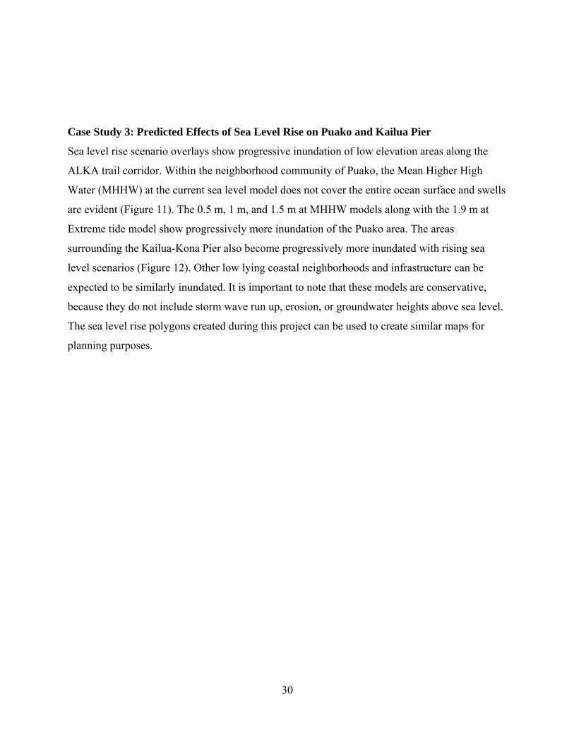
Case Study 3: Predicted Effects of Sea Level Rise on Puako and Kailua Pier
Sea level rise scenario overlays show progressive inundation of low elevation areas along the
ALKA trail corridor. Within the neighborhood community of Puako, the Mean Higher High
Water (MHHW) at the current sea level model does not cover the entire ocean surface and swells
are evident (Figure 11). The 0.5 m, 1 m, and 1.5 m at MHHW models along with the 1.9 m at
Extreme tide model show progressively more inundation of the Puako area. The areas
surrounding the Kailua-Kona Pier also become progressively more inundated with rising sea
level scenarios (Figure 12). Other low lying coastal neighborhoods and infrastructure can be
expected to be similarly inundated. It is important to note that these models are conservative,
because they do not include storm wave run up, erosion, or groundwater heights above sea level.
The sea level rise polygons created during this project can be used to create similar maps for
planning purposes.

31
Figure 11: Sea level rise scenarios at Puako where blue represents water surfaces. Note that the Mean Higher High Water (MHHW) model at current sea levels does not cover all of the ocean surface and swells are evident. The 0.5 m, 1 m, and 1.5 m at MHHW models along with the 1.9 m at Extreme tide model show progressively more inundation of the Puako area.

32
Figure 12: Inundation at Kailua-Kona Pier and surrounding areas under various sea level rise scenarios. All scenarios are at Extreme high tide.

33
CONCLUSION
Incorporating detailed elevation data and sea level rise predictions in coastal planning
should aid in long-term management of both developed and natural areas. In particular this
project aims to identify key areas to preserve for maintaining environmental and cultural
integrity in the future. For example, while some features such as individual anchialine pools will
be inundated, anchialine pool, fishpond and wetland habitats will emerge or shift in the
landscape. Protecting future inundation areas from development will conserve valuable habitat
and will eliminate the need to repair or relocate infrastructure placed in these areas.
The models used here are a conservative method for estimating inundation and do not
include storm run up, erosion, changes in sediment deposition, and geologic activities which will
have additional effects on Hawaii’s future shorelines. Recently Marrack (2014) has developed
methods to incorporate observed groundwater levels into geospatial models. Models that
incorporate groundwater into sea level rise scenarios are available for the Kawaihae to South
Kona section of the ALKA corridor.
The goal of this project is to share sea level rise inundation and error polygons with NPS
staff as well as various public and private partners so that they can plan for future conditions.
This visualization tool will also be helpful in educating the public about the effects of global
warming and resulting sea level rise. GIS data are available through the National Park Service at
ALKA.
ACKNOWLEDGEMENTS
We are grateful to Rick Gmirkin, Aric Arakaki, Sallie Beavers, Nancy Erger, Darcy Hu, and
others for their support. We are also grateful to Maggi Kelly, Chip Fletcher’s Lab group, Kirk
Waters, and Maria Caffrey for their comments on the project and manuscript. Finally, Ed
Carlson, John Marra, and Doug Harper generously conducted and shared data from surveys of
National Geodetic Survey benchmarks. This project is a Californian Cooperative Ecosystem
Studies Unit Project of the National Park Service and the University of California Regents at
Berkeley (Task Agreement #J8C07100018). The funding sources had no role in the study design,
collection, analysis and interpretation of data.

34
REFERENCES (ASPRS) American Society of Photogrammetry and Remote Sensing, 2004. ASPRS Guidelines
Vertical Accuracy Reporting for LiDAR Data V1.0.” http://www.asprs.org/Standards. Bauer, G., 2003. A Study of the Ground-water conditions in North and South Kona and South
Kohala Districts Island of Hawaii, 1991-2002. Honolulu, Hawaii: Department of Land and Natural Resources, Commission on Water Resource Management, PR-2003-01. 95p.
Bjerklie, D.M., Mullaney, J.R., Stone, J.R., Skinner, B.J., and Ramlow, M.A., 2012. Preliminary
investigation of the effects of sea-level rise on groundwater levels in New Haven, Connecticut. Reston, Virginia: U.S. Geological Survey Open-File Report 2012–1025, 46p.
Cayan, D., Tyree, M., Dettinger, M., Hidalgo, H., Das, T., Maurer, E., Bromirski, P., Graham, N.
and Flick, R., 2009. Climate Change Scenarios and Sea Level Rise Estimates for California, 2008 Climate Change Scenarios Assessment. California Climate Change Center. CEC‐500‐2009‐014‐F.
Church, J. A. and White, N.J., 2011. Sea-level rise from the late 19th to the early 21st Century. Surveys in Geophysics. doi:10.1007/s10712-011-9119-1.
Cooper, H.M., Chen, Q., Fletcher, C.H., and Barbee, M.M., 2013. Assessing vulnerability due to sea-level rise in Maui, Hawaii using LiDAR remote sensing and GIS. Climatic Change, 116(3), 547-563.
Dasgupta, S., LaPlante, B.,Meisner, C., Wheeler, D., and Yan, J., 2009. The impact of sea level
rise on developing countries: a comparative analysis. Climatic Change. 93, 379-388. Dewberry and Davis., 2007. Lidar QaQc Report Hawaii TO26: Big Island, Oahu, and Kauai
August 2007. FEMA-Lidar 2006 data report. 43 pgs.
Gesch, D.B., 2009. Analysis of LiDAR elevation data for improved identification and delineation of lands vulnerable to sea-level rise. Journal of Coastal Research, SI(53), 49-58. http://topotools.cr.usgs.gov/pdfs/jcr_gesch_SI53.pdf
Geselbracht, L., Freeman, K., Kelly, E., Gordon, D.R., and Putz, F.E. 2011. Retrospective and prospective model simulations of sea level rise impacts on Gulf of Mexico coastal marshes and forests in Waccasassa Bay, Florida. Climatic Change. 107:35–57. DOI 10.1007/s10584-011-0084-y
Grannis, J., 2011. Adaptation Tool Kit:Sea-Level Rise and Coastal Land Use How Governments Can Use Land-Use Practices to Adapt to Sea-Level Rise. Georgetown Climate Center. 90 pgs. http://www.georgetownclimate.org/resources/adaptation-tool-kit-sea-level-rise-and-coastal-land-use

35
Heberger, M., Cooley, H., Herrera, P., Gleick, P. H. and Moore,E.. 2009. The impacts of sea level rise on the California Coast. California Climate Change Center. 100p. CEC-500-2009-024-F. http://www.energy.ca.gov/2009publications.
Holthuis, L.B., 1973. Caridean shrimps found in land-locked saltwater pools at four Indo-west
Pacific localities (Sinai Peninsula, Funafuti Atoll, Maui and Hawaii Islands), with the description of one new genus and four new species. Zool. Verhadenlingen 128: 3-55.
(IPCC) Intergovernmental Panel on Climate Change, 2013. Climate Change 2013: The Physical
Science Basis. Contribution of Working Group I to the Fifth Assessment Report of the Intergovernmental Panel on Climate Change [Stocker, T.F., D. Qin, G.-K. Plattner, M. Tignor, S. K. Allen, J. Boschung, A. Nauels, Y. Xia, V. Bex and P.M. Midgley (eds.)]. Cambridge University Press, Cambridge, United Kingdom and New York, NY, USA
Knee, K., Street, J., Grossman, E., and Paytan, A., 2008. Submarine ground-water discharge and
fate along the coast of Kaloko-Honokohau National Historical Park, Island of Hawaii-Part 2, Spatial and temporal variations in salinity, radium-isotope activity, and nutrient concentrations in coastal waters, December 2003-April 2006. U.S. Geological Survey Scientific Investigations Report 2008-5128, 31p.
Knowles, N., 2010. Potential Inundation Due to Rising Sea Levels in the San Francisco Bay
Region. San Francisco Estuary and Watershed Science, 8:1. Available at http://escholarship.org/uc/search?entity=jmie_sfews;volume=8;issue=1
Maciolek, J.A., and Brock, R.E., 1974. Aquatic survey of the Kona coast ponds, Hawaii Island. Honolulu, Hawaii: University of Hawaii Sea Grant, Report AR74-04, Grant No. 04-3-158-29. 76p.
Marcy, D., Brooks, W., Draganov, K., Hadley, B., Haynes, C., Herold, N., McCombs, J., Pendleton, M., Ryan, S., Schmid, K., Sutherland, M., and Waters, K., 2011. “New Mapping Tool and Techniques for Visualizing Sea Level Rise and Coastal Flooding Impacts.” In Proceedings of the 2011 Solutions to Coastal Disasters Conference, Anchorage, Alaska, June 26 to June 29, 2011, edited by Louise A. Wallendorf, Chris Jones, Lesley Ewing, and Bob Battalio, 474–90. Reston, VA: American Society of Civil Engineers
Marra, J. J., Merrifield, M.A., and Sweet, W.V., 2012. Sea Level and Coastal Inundation on Pacific Islands. In V. W. Keener, J. J. Marra, M. L. Finucane, D. Spooner, & M. H. Smith (Eds.), Climate Change and Pacific Islands: Indicators and Impacts. Report for the 2012 Pacific Islands Regional Climate Assessment (PIRCA). Washington, DC: Island Press.
Marrack, L. and Beavers. S., 2011 (In press). Inventory and Assessment of Anchialine Pool
Habitats in Kaloko-Honokōhau National Historical Park. CESU Technical Report –U.of Hawaii & NPS: 58p
36
Marrack, L., 2014. Incorporating groundwater levels into sea level detection models for Hawaiian anchialine pool ecosystems. Journal of Coastal Research, preprint available at: http://www.jcronline.org/doi/abs/10.2112/JCOASTRES-D-13-00043.1
McGee Surveying Consulting, 2007. Survey Report for the Quality Control - Quality Assurance
Data Collection for Dewberry and Davis on the Island of Hawaii Along the Westerly and Southerly Coastlines. Santa Barbara, California: Project: EMF-2003-CO-0047. 5p.
Meyssignac, B. and Cazenave, A., 2012. Sea level: A review of present-day and recent-past
changes and variability.- Journal of Geodynamics. 58:96-109. Moore, J.G. and Clague, D.A., 1992. Volcano growth and evolution of the island of Hawaii. -
Geol. Soc. Am. Bull.. 104: 1471–1484. Nicholls, R.J., and Cazenave, A., 2010. Sea-level rise and its impact on coastal zones. Science,
328, 1517–1520. (NOAA) National Oceanic and Atmospheric Administration, 2012.
http://www.csc.noaa.gov/digitalcoast/data/coastalLiDAR/index.html NOAA, 2011. Kawaihae Tidal Benchmark Datum Page. http://tidesandcurrents.noaa.gov
Oki, D., 1999. Geohydrology and numerical simulation of the ground-water flow system of Kona, Island of Hawaii. Reston, Virginia: U.S. Geological Survey, Water-Resources Investigation Report 99-4073,70p.
Parris, A., Bromirski, P., Burkett, V., Cayan, D., Culver, M., Hall, J., Horton, R., Knuuti, K.,
Moss, R., Obeysekera, J., Sallenger, A., and Weiss, J. 2012. Global Sea Level Rise Scenarios for the US National Climate Assessment. NOAA Tech Memo OAR CPO-1. 37 pp. http://www.cpo.noaa.gov/sites/cpo/Reports/2012/NOAA_SLR_r3.pdf
Rignot, E. , Velicogna, I., Van den Broeke, M.R., Monaghan, A., and Lenaerts, J., 2011.
Acceleration of the contribution of the Greenland and Antarctic ice sheets to sea level rise. Geophysical Research Letters, Vol 38, L05503, (doi:10.1029/2011GL046583).
Reynolds, M.H., Berkowitz, P., Courtot, K.N., and Krause, C.M., (eds.), 2012. Predicting sea-
level rise vulnerability of terrestrial habitat and wildlife of the Northwestern Hawaiian Islands. Reston, Virginia: U.S. Geological Survey Open-File Report 2012–1182, 139p.
Rotzoll, K. and Fletcher, C.H., 2013. Assessment of groundwater inundation as a consequence of
sea-level rise. Nature Climate Change. Online publication, DOI: 10.1038/NCLIMATE1725
State of Massachusetts Executive Committee of Energy and Environmental Affairs. 2011. Massachusetts Climate Change Adaptation Report. 121 pgs. http://www.mass.gov/eea/docs/eea/energy/cca/eea-climate-adaptation-report.pdf

37
Titus, J.G., Hudgens, D.E., Trescott, D.L., Craghan, M., Nuckols, W.H.,. Hershner, C.H.,. Kassakian, J. M., Linn, C.J., Merritt, P.G., McCue, T.M., O'Connell, J.F., Tanski, J. and Wang, J., 2009. State and Local Governments Plan for Development of Most Land Vulnerable to Rising Sea Level along the U.S. Atlantic Coast, Environmental Research Letters. 4 044008. (doi: 10.1088/1748-9326/4/4/044008).
(USFWS) United States Fish and Wildlife Service, 2011. Endangered and Candidate Species Reports. Accessed at http://www.fws.gov/endangered/index.html.
Vermeer, M. and Rahmstorf S., 2009. Global sea level linked to climate change. PNAS 106. pp.
21527-21532.
Vitousek, S., Barbee, M.M., Fletcher, C.H., and Genz, A.S., 2010. Pu'ukohola Heiau National Historic Site and Kaloko-Honokohau Historical Park, Big Island of Hawai‘i Coastal: Hazard Analysis. Natural Resource Technical Report NPS/NRPC/NRTR/GRD-2010/387. National Park Service, Fort Collins, Colorado.
Williams, S.J., 2013. Sea-level rise implications for coastal regions. In: Brock, J.C.; Barras, J.A., and Williams, S.J. (eds.), Understanding and Predicting Change in the Coastal Ecosystems of the Northern Gulf of Mexico. Journal of Coastal Research, Special Issue No. 63, pp. 184–196.
Zhong, S., and Watts, A.B., 2002. Constraints on the dynamics of mantle plumes from uplift of
the Hawaiian Islands. - Earth and Planetary Science Letters. 203:105-116.

38
Appendix 1: Key for GIS shapefiles produced to visualize various sea level rise scenarios under various high tides. Table indicates shapefile name, spatial coverage, sea level rise scenario and tide state. Error polygons can be used in conjunction with the associated scenario files and represent the 95th percentile confidence due to LiDAR measurement error. Sea level rise scenarios with groundwater incorporate groundwater into flooding models (Marrack 2014). Hawaii Volcanoes National Park is identified as HAVO in the table.
Type File Name Location SLR Scenario Tide
Sea Level Rise Scenarios Nth_Koh_0.5mMHHW North Kohala 0.5 meters MHHW Nth_Koh_0.5mExt North Kohala 0.5 meters Extreme annual tide Nth_Koh_1mMHHW North Kohala 1 meters MHHW Nth_Koh_1mExt North Kohala 1 meters Extreme annual tide Nth_Koh_1.5mMHHW North Kohala 1.5 meters MHHW Nth_Koh_1.5mExt North Kohala 1.5 meters Extreme annual tide Nth_Koh_1.9mMHHW North Kohala 1.5 meters MHHW Nth_Koh_1.9mExt North Kohala 1.9 meters Extreme annual tide Kona_0.5m_MHHW Kawaihae to Kahauloa 0.5 meters MHHW Kona_0.5m_Ext Kawaihae to Kahauloa 0.5 meters Extreme annual tide Kona_1m_MHHW Kawaihae to Kahauloa 1 meters MHHW Kona_1m_Ext Kawaihae to Kahauloa 1 meters Extreme annual tide Kona_1.5m_MHHW Kawaihae to Kahauloa 1.5 meters MHHW Kona_1.5m_Ext Kawaihae to Kahauloa 1.5 meters Extreme annual tide Kona_1.9m_MHHW Kawaihae to Kahauloa 1.9 meters MHHW Kona_1.9m_Ext Kawaihae to Kahauloa 1.9 meters Extreme annual tide Sth_0.5m_MHHW Kahauloa to HAVO 0.5 meters MHHW Sth_0.5m_Ext Kahauloa to HAVO 0.5 meters Extreme annual tide Sth_1m_MHHW Kahauloa to HAVO 1 meters MHHW Sth_1m_Ext Kahauloa to HAVO 1 meters Extreme annual tide Sth_1.5m_MHHW Kahauloa to HAVO 1.5 meters MHHW Sth_1.5m_Ext Kahauloa to HAVO 1.5 meters Extreme annual tide Sth_1.9m_MHHW Kahauloa to HAVO 1.9 meters MHHW Sth_1.9m_Ext Kahauloa to HAVO 1.9 meters Extreme annual tide

39
Appendix 1 : continued Error Polygons (95th percentile confidence : + 0.25m)
er_Koh_0.5mMHHW North Kohala 0.5 meters MHHW er_Koh_0.5mEXT North Kohala 0.5 meters Extreme annual tide er_Koh_1mMHHW North Kohala 1 meters MHHW er_Koh_1mEXT North Kohala 1 meters Extreme annual tide er_Koh_1.5mMHHW North Kohala 1.5 meters MHHW er_Koh_1.5mEXT North Kohala 1.5 meters Extreme annual tide er_Koh_1.9mMHHW North Kohala 1.5 meters MHHW er_Koh_1.9mEXT North Kohala 1.9 meters Extreme annual tide er_Kona_0.5mMHHW Kawaihae to Kahauloa 0.5 meters MHHW er_Kona_0.5mEXT Kawaihae to Kahauloa 0.5 meters Extreme annual tide er_Kona_1mMHHW Kawaihae to Kahauloa 1 meters MHHW er_Kona_1mEXT Kawaihae to Kahauloa 1 meters Extreme annual tide er_Kona_1.5mMHHW Kawaihae to Kahauloa 1.5 meters MHHW er_Kona_1.5mEXT Kawaihae to Kahauloa 1.5 meters Extreme annual tide er_Kona_1.9mMHHW Kawaihae to Kahauloa 1.9 meters MHHW er_Kona_1.9mEXT Kawaihae to Kahauloa 1.9 meters Extreme annual tide er_Sth_0.5mMHHW Kahauloa to HAVO 0.5 meters MHHW er_Sth_0.5mEXT Kahauloa to HAVO 0.5 meters Extreme annual tide er_Sth_1mMHHW Kahauloa to HAVO 1 meters MHHW er_Sth_1mEXT Kahauloa to HAVO 1 meters Extreme annual tide er_Sth_1.5mMHHW Kahauloa to HAVO 1.5 meters MHHW er_Sth_1.5mEXT Kahauloa to HAVO 1.5 meters Extreme annual tide er_Sth_1.9mMHHW Kahauloa to HAVO 1.9 meters MHHW er_Sth_1.9mEXT Kahauloa to HAVO 1.9 meters Extreme annual tide
Sea Level Rise Scenarios with Groundwater
GWKona_0.5mMHHW Kawaihae to Kailua Bay 0.5 meters MHHW
GWKona_0.5mEXT Kawaihae to Kailua Bay 0.5 meters Extreme annual tide
GWKona_1mMHHW Kawaihae to Kailua Bay 1 meters MHHW
GWKona_1mEXT Kawaihae to Kailua Bay 1 meters Extreme annual tide
GWKona_1.5mMHHW Kawaihae to Kailua Bay 1.5 meters MHHW
GWKona_1.5mEXT Kawaihae to Kailua Bay 1.5 meters Extreme annual tide
40
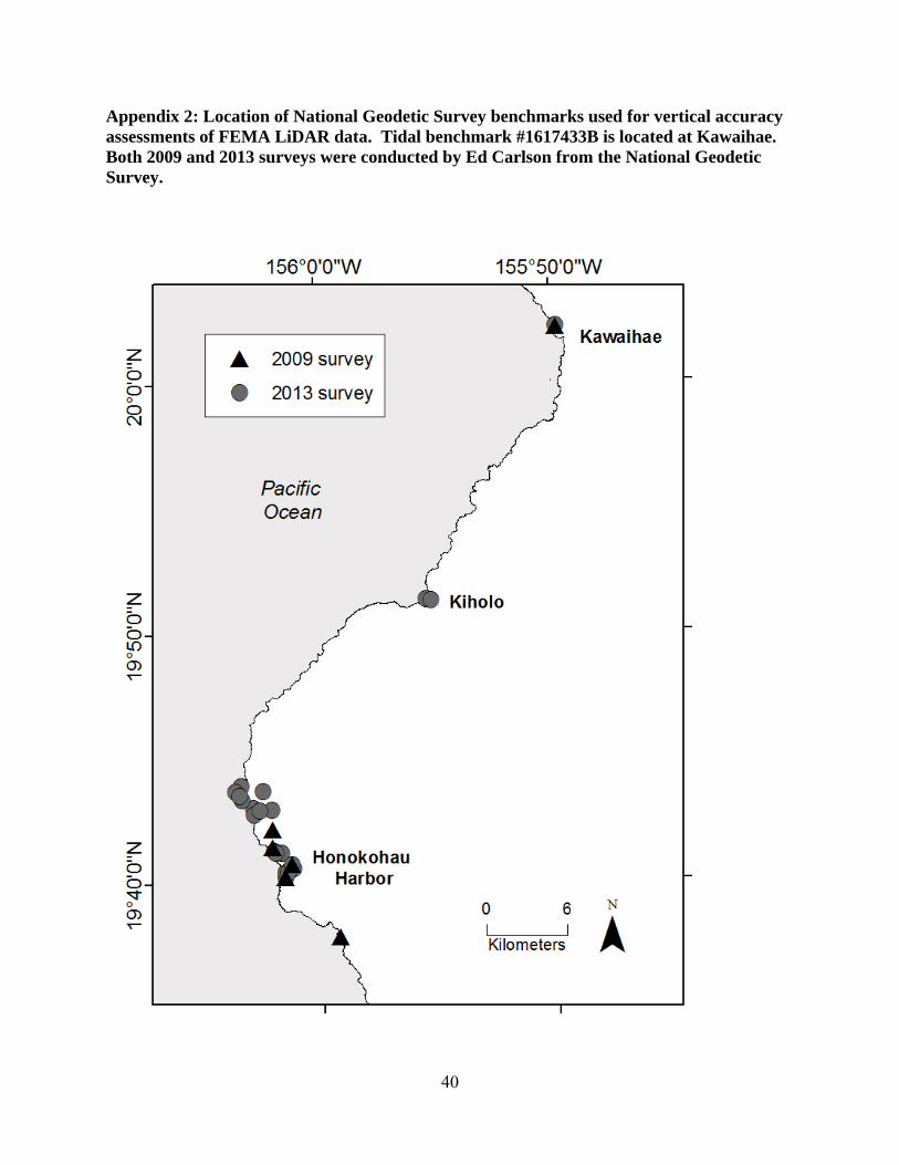
Appendix 2: Location of National Geodetic Survey benchmarks used for vertical accuracy assessments of FEMA LiDAR data. Tidal benchmark #1617433B is located at Kawaihae. Both 2009 and 2013 surveys were conducted by Ed Carlson from the National Geodetic Survey.