The Growth Contribution of Colonial Indian Railwaysin Comparative Perspective∗

Dan Bogart† Latika Chaudhary‡ Alfonso Herranz-Loncán§

February 2015

Abstract

It is widely recognized that railways were one of the most important drivers ofeconomic growth in the 19th and 20th century, but it is less recognized that railwayshad a different impact across countries. In this paper, we first estimate the growthimpact of Indian railways, one of the largest networks in the world circa 1900. Then,we show railways made a smaller contribution to income per-capita growth in Indiacompared to the most dynamic Latin American economies between 1860 and 1912. Thesmaller contribution in India is related to four factors: (1) the smaller size of railwayfreight revenues in the Indian economy, (2) the higher elasticity of demand for freightservices, (3) lower wages, and (4) higher fares. Our results suggest large disruptivetechnologies such as railways and other communication technologies can generate hugeresources savings, but may not have large growth impacts.

Keywords: Railways, Social Savings, ICT, India, Growth Accounting

JEL Codes: N7, O47, P52, R4

∗We thank seminar participants at UC Irvine and Yale’s conference on New Research in South AsianEconomic History. All errors are our own.†Associate Professor, Department of Economics, UC Irvine, Email:dbogart@uci.edu‡Associate Professor, Graduate School of Business and Public Policy, Naval Postgraduate School,

Email:lhartman@nps.edu§Associate Professor, Department of Economic History and Institutions, University of Barcelona,

Email:alfonso.herranz@ub.edu

1 Introduction

Advances in information and communications technology (ICT) have transformed economiesaround the world. Similar to cell phones and the internet of today, railways were themost important ICT of the 19th century. Soon after the early construction of railwaysin Britain, steam powered railways spread from North-West Europe to Asia and LatinAmerica beginning in the 1830s. In many countries railways were the engine of growthlowering transport costs, reducing price dispersion, integrating markets, extending frontiersand increasing incomes. But, the transformative and often disruptive impact of railwayswas not uniform across time and space. Some countries experienced a large economic bang,while in others the effects were more understated.

In this paper, we estimate the growth contribution of colonial Indian railways and com-pare it to the performance of railways in four large Latin American economies between thelate 19th and early 20th century. The time frame captures the development of the rail net-work in these countries and ends just before World War 1. India offers a unique perspectivebecause the existing evidence paints a mixed picture. On the one hand India fell behindother economies during the height of the ‘railway era’ from 1860 to 1912. India’s per-capitaincome increased just 31% between 1870 and 1910 (from $533 to $697), whereas the LatinAmerican average increased by 110% (from $742 to $1562).1 Many scholars argue Britishcolonial policies were the root cause of the decline (for example, Bagchi 1982). Such ar-guments specific to railways point to high fares, high freight rates and the construction ofseveral unprofitable railways (Hurd 1983, 2007, Sweeney 2011). On the other hand Indianrailways are thought to be a rare success story for the British Raj. Railways transformedIndia from many segmented markets separated by high transportation costs to an economywith local centers linked by rail to each other and the world. According to Donaldson (2012),railways raised agricultural incomes by 16% in districts with access to the network. And,Bogart and Chaudhary (2013) find that the growth and level of Indian railways’ total fac-tor productivity was large compared to both developed and developing economies by 1913.Comparing India to similar economies in Latin America can help shed light on this puzzle,and more generally the different effects of ICTs.

We choose Mexico, Argentina, Brazil and Uruguay (LA4) as the comparison set becauselike India these were large economies with extensive rail networks by 1912. LA4 accountedfor 65 percent of Latin American GDP, 59 percent of the population and 79 percent of LatinAmerican railway mileage. With the exception of Brazil, LA4 were among the few Latin

1The income per-capita data are from Maddison (2001), reported in 1990 purchasing power parity (PPP)adjusted dollars.

1

American countries to build integrated national railway networks. Similar to India, the LA4economies heavily relied on primary exports in the 19th century. But unlike India, theirrailways were mostly private, they were not colonies and had lower population density (andconsequently higher wages) than India.

Our estimation is based on the growth accounting framework, which incorporates the so-cial savings methodology. Social savings are the classic metric for evaluating the contributionof railways following seminal work by Fogel (1964) and Fishlow (1966). The social savingscapture the value of lost resources had the quantity of railway traffic been transported atthe prices of pre-railway transport in a benchmark year, say 1912. In a series of influentialarticles Crafts (2004a,b) extended social savings to a growth accounting framework. Accord-ing to the basic growth accounting identity, income per-capita growth can be divided intoincreases in physical capital stock per-capita and “crude” total factor productivity growth(the so-called “Solow residual”). Crafts measured the contribution of railways to each one ofthe components by estimating a railway capital term representing the embodiment of rail-way technology in the capital stock, and a railway TFP term capturing the resource savingsfrom lower transport costs. As Crafts shows, under competitive assumptions the TFP termis equivalent to the additional consumer surplus generated by railways, which in turn is thesame as the social savings corrected by the elasticity of demand.

We extend the social savings methodology in several important ways. First, we decom-pose the savings for freight into two terms: (1) the share of railway freight revenues in GDPand (2) the ratio of pre-existing freight rates to railway rates. The share term can be calledthe “railway penetration effect” as it captures the degree to which individuals and firms usedrailway services. The ratio term can be called the “relative productivity effect” as it measuresto what degree railways reduced freight rates relative to the alternative technology. Second,we decompose the savings from passengers into similar terms, and go further by decompos-ing the time cost of traveling, which depends on the hourly wage and the average speed oftrains and alternatives. Third, we incorporate the profits of railways, which represent thepart of TFP growth retained by railway companies and not transferred to users via lowerfares. Quantifying the importance of the various components of the social savings providesan important step in explaining why a communication technology like railways had a largeimpact in one economy, and a smaller impact in another.

The main finding is that railways accounted for a large share of Indian GDP per capitagrowth, but they made a smaller growth contribution than railways in the most successfulLatin American economies. Our preferred estimates show that Indian railways contributed0.29 percentage points to annual income per-capita growth from the mid 19th to the early

2

20th century, larger than Uruguay (0.11%), similar to Brazil (0.31%), but less than Argentina(0.65%) and Mexico (0.53%). We perform several robustness checks and the same rankingof India’s growth contribution carries through. One reaches a different conclusion regardingthe contribution of railways as a share of total income per-capita growth. Railways accountfor 73% of all income per-capita growth in India, similar to Brazil at 62%. In contrast,railways account for a smaller share in Argentina (22%), Mexico (24%) and Uruguay (8%).In Argentina and Mexico the large savings provided by railways appear relatively smallbecause income per-capita growth rates averaged 2.6% between the late 19th and early 20th

century. India and Brazil were stagnant in the same period with income per-capita growthrates averaging only 0.5%.

What explains the differences across countries? The decomposition exercise for freightsuggests Indian freight revenues were smaller as a share of GDP than most LA4, which lowersthe social savings. But, pre-existing freight rates were much higher in India compared torailway rates, which increases the socials savings. We also find that India had a relativelyelastic demand for freight services, and a higher elasticity lowers social savings becausethe latter must be adjusted down to estimate the additional consumer surplus. On netthe relatively elastic demand for freight services in India combined with the smaller freightrevenues contributed to lower consumer surplus from railways because these two factorsmore than compensate for the difference in freight rates between pre-existing and railwaytransport.

For passenger travel, the decomposition shows India had a relatively high penetrationrate. Lower class passenger travel was huge in India by 1913. However, lower wages in Indiareduced the time cost of traveling and hence the social savings. Indian railway fares werealso high compared to wages, which further lowered the social savings. Finally, we find thatIndian railways were profitable in 1912 compared to Argentina and Mexico where railwaysearned zero or negative profits. Given the ownership structure of Indian railways, the profitslargely went to the colonial Government and to some degree offset tax revenues on Indians.

Our paper contributes to the large literature on the economic impact of railways.2 Weoffer a detailed analysis of the social savings from Indian railways before World War I. Indiais an important case because it had the largest railway system in the developing world inthis period. Our results also speak to the literature on the Indian economy. In recentpapers, scholars have studied the historical roots of the service sector (Broadberry andGupta 2010), and the long-run adverse impact of direct colonial rule (Iyer 2010). We add to

2This literature began with the classic works by Fogel (1964) and Fishlow (1965). It has continued withstudies by Coatsworth (1981), Summerhill (2000, 2003), Crafts (2004a), Leunig (2006), Herranz-Loncán(2006, 2011b, 2014), and Donaldson and Hornbeck (2013) among others.

3

this growing literature by studying one of the leading sectors of the economy. Our bottomline is that railways were the most important driver of economic growth in India before 1913.This is perhaps unsurprising because productivity growth in agriculture, the largest sectorof the Indian economy was stagnant in this period (Broadberry and Gupta 2010). But,railways also contributed far less to Indian economic growth compared to other countries.Our decomposition exercises suggest India’s economic structure is one reason. The moremodest penetration of railways suggests that Indian workers and communities did not fullyassimilate into the global economy when railways arrived. India’s low wages were one keyreason because they lowered the time savings of railways. There were also potential policymistakes. Consistent with the extraordinary profits earned by Indian railways compared toLA4, fares and freight rates were high. Given the colonial Government’s regulatory poweron Indian railways, this would be a failure of colonial policy.

Finally, our results contribute to the literature on ICT. Researchers have found a largegrowth contribution from ICT in developed and developing countries (Roller and Waverman2001, Aker and Mbiti 2010). The estimates presented here on railways are consistent withcommunications technologies playing a large and important role. That said, our findingssuggest that where railways were not accompanied by other structural changes, they endedup accounting for an exceedingly large share of a small total per-capita growth rate.

The rest of the paper is organized as follows. Section 2 provides a brief background onIndian railways. We describe the social savings methodology in Section 3. Section 4 detailsthe assumptions and calculations of the different components of the growth contribution.Section 5 puts Indian railways in a comparative perspective and Section 6 concludes.

2 Background on Indian Railways

By most accounts India’s transportation sector was costly and unproductive at the beginningof the railway era. India had many rives, but they were often not navigable or seasonal asin the case of the Ganges and the Indus. India had a long coast line, but shipping washampered by seasonality and changing winds. In terms of investments in roads and canals,India was clearly behind Western countries.

Railways changed India’s transport sector dramatically. British mercantile firms wereamong the early advocates for railway construction in India (Thorner 1955). They arguedrailways would lower transport costs, allow access to raw Indian cotton and open Indianmarkets to British manufactured goods. The first passenger line measuring 32 km openedin 1853. The size of the network grew rapidly in the 1880s and 1890s with track km

4

increasing from 15,000 in 1880 to 54,000 in 1913 (Bogart and Chaudhary 2015). Networkexpansion continued after 1913 when we end our analysis, but the pace of developmentslowed. Although economic motives spurred the initial wave of construction, political anddevelopment concerns became important beginning in the 1870s. Railways were built inpart to mitigate the effects of famines, put down rebellions, and defend the frontier.

By the early 20th century railways spread to most parts of India as seen in Figure 1showing the network in 1909 (color coded for each railway system). The first passenger lineconnected the port of Bombay to the interior. Similar connections were soon made betweenthe ports of Calcutta, Madras, and Karachi and their hinterlands. A dense interior networkwas constructed between Delhi and Calcutta along the Ganges River, where railways servedlong-standing population centers. However, outside of the links with Delhi there were fewinterior-to-interior connections. Much of central and southern India was distant from arailway.

The construction and management of colonial railways involved private British compa-nies, the colonial Government of India (GOI), and Indian Princely States. In the first phaseup to 1869, private British companies constructed and managed trunk lines under a pub-lic guarantee. Such guarantees for railway construction were common in the 19th century.For example, railway companies in Brazil received guarantees of around 7%, large than the5% in India. In the second phase, the GOI began constructing and managing railways inthe 1870s. The third phase, beginning in the early 1880s, involved hybrid public-privatepartnerships between the GOI as majority owner of the line and private companies. In thefourth phase, starting in 1924, the GOI began taking over railway operations completingnationalization.3

The structure of the economy matched the flow of goods on the railways. The largesttraffic category was agriculture (see Figure 2).4 It included commodities like grain, oilseeds,pulses, cotton, tea, and jute. Agriculture, the largest source of Indian exports, was the coreof traffic between the hinterlands and the ports. The second largest traffic category wasminerals, with coal being by far the largest. Coal was shipped internally and was used byrailways distant from mines, and to a lesser extent in manufacturing. Salt, another importantcommodity in internal trade, was also part of the mineral category. In comparison, traffic inmanufactured goods was small averaging 5% between 1883 and 1912. Some of these goodswere Indian made, but many were imports.

Several studies have looked at the economic impact of Indian railways. Early work by3See Sanyal (1930) for a detailed overview of the regulatory history of Indian railways.4The commodity data are from Morris and Dudley (1975, p. 39).

5

Hurd (1975) and McAlpin (1974) found less price dispersion and more price convergencein railway districts compared to non-railway districts and as railways expanded over time.These studies and those by Studer (2008) suggest a large impact of railways on marketintegration. By contrast, Andrabi and Kuehlwein (2010) argue against a large impact.They regress the price gap for wheat and rice between major Indian cities on an indicatorvariable for whether a railway connected the two cities in each year. Unlike the earlierstudies, they focus on changes in price gaps before and after railways link a market pair.Their estimates imply that railways explain only 20 percent of the overall 60 percent decreasein price dispersion between the 1860s and 1900s. In a similar vein, Collins (1999) examineswages and finds limited evidence of convergence during the key decades of railway expansion.

Recently, Donaldson (2012) taking a theoretically grounded and rigorous empirical ap-proach finds large effects of railways on trade costs and agricultural incomes. He exploitsvariation in salt prices, a better proxy for trade costs compared to wheat or rice prices usedin other studies, because salt was produced in one district and transported to others. Usingpanel and IV regressions, he finds the arrival of railways increased agricultural incomes by16% in a district-level analysis. Significantly for our paper, Donaldson estimates the degreeto which railways reduced trade costs relative to carts and boats using differences in saltprices across districts.

Unlike these studies, we take a macro approach and estimate the impact of Indian rail-ways by measuring their contribution to the increase in capital stock per-capita and TFP ofthe economy. The latter is based on an estimation of the social savings of railways. As is wellknown, the social savings compare the freight rates of railways with some alternative, likebullock carts, and use these figures to measure the income loss from shipping railway trafficwith pre-railway transport technology. The main precedent of our work is Hurd (1983), whoestimated the social savings on Indian freight traffic to be 1.2 billion rupees or 9 percent ofnational income in 1900. But, Hurd’s calculation is not detailed. He does not specify theassumptions, sources or sample. We combine a social savings calculation with the recentmethodology developed by Crafts (2004a) to estimate a precise impact of Indian railwaysby 1912 when most of the network was complete. We then compare the Indian experienceto LA4 for which such estimates have already been compiled using the same methodology(Herranz-Loncán 2014). This exercise puts the Indian experience in a global perspectiveand offers a much needed macro view.

6

3 Methodology

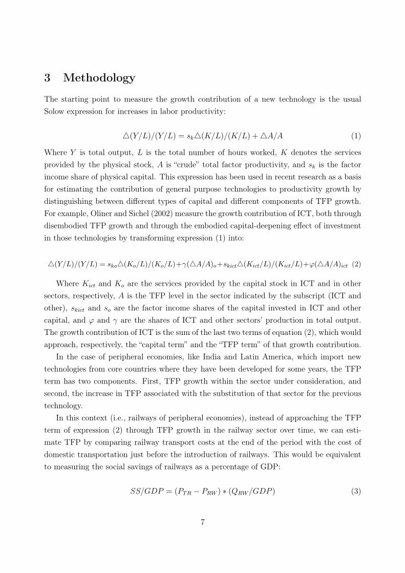
The starting point to measure the growth contribution of a new technology is the usualSolow expression for increases in labor productivity:

4(Y/L)/(Y/L) = sk4(K/L)/(K/L) +4A/A (1)

Where Y is total output, L is the total number of hours worked, K denotes the servicesprovided by the physical stock, A is “crude” total factor productivity, and sk is the factorincome share of physical capital. This expression has been used in recent research as a basisfor estimating the contribution of general purpose technologies to productivity growth bydistinguishing between different types of capital and different components of TFP growth.For example, Oliner and Sichel (2002) measure the growth contribution of ICT, both throughdisembodied TFP growth and through the embodied capital-deepening effect of investmentin those technologies by transforming expression (1) into:

4(Y/L)/(Y/L) = sko4(Ko/L)/(Ko/L)+γ(4A/A)o+skict4(Kict/L)/(Kict/L)+ϕ(4A/A)ict (2)

Where Kict and Ko are the services provided by the capital stock in ICT and in othersectors, respectively, A is the TFP level in the sector indicated by the subscript (ICT andother), skict and so are the factor income shares of the capital invested in ICT and othercapital, and ϕ and γ are the shares of ICT and other sectors’ production in total output.The growth contribution of ICT is the sum of the last two terms of equation (2), which wouldapproach, respectively, the “capital term” and the “TFP term” of that growth contribution.

In the case of peripheral economies, like India and Latin America, which import newtechnologies from core countries where they have been developed for some years, the TFPterm has two components. First, TFP growth within the sector under consideration, andsecond, the increase in TFP associated with the substitution of that sector for the previoustechnology.

In this context (i.e., railways of peripheral economies), instead of approaching the TFPterm of expression (2) through TFP growth in the railway sector over time, we can esti-mate TFP by comparing railway transport costs at the end of the period with the cost ofdomestic transportation just before the introduction of railways. This would be equivalentto measuring the social savings of railways as a percentage of GDP:

SS/GDP = (PTR − PRW ) ∗ (QRW/GDP ) (3)

7

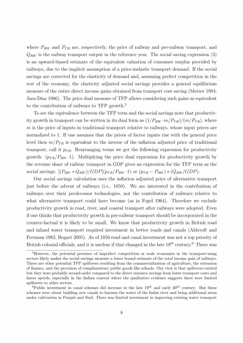
where PRW and PTR are, respectively, the price of railway and pre-railway transport, andQRW is the railway transport output in the reference year. The social saving expression (3)is an upward-biased estimate of the equivalent valuation of consumer surplus provided byrailways, due to the implicit assumption of a price-inelastic transport demand. If the socialsavings are corrected for the elasticity of demand and, assuming perfect competition in therest of the economy, the elasticity adjusted social savings provides a general equilibriummeasure of the entire direct income gains obtained from transport cost saving (Metzer 1984;Jara-Díaz 1986). The price dual measure of TFP allows considering such gains as equivalentto the contribution of railways to TFP growth.5

To see the equivalence between the TFP term and the social savings note that productiv-ity growth in transport can be written in its dual form as (1/PRW–m/PTR)/(m/PTR), wherem is the price of inputs in traditional transport relative to railways, whose input prices arenormalized to 1. If one assumes that the prices of factor inputs rise with the general pricelevel then m/PTR is equivalent to the inverse of the inflation adjusted price of traditionaltransport, call it pTR. Rearranging terms we get the following expression for productivitygrowth: (pTR/PRW–1). Multiplying the price dual expression for productivity growth bythe revenue share of railway transport in GDP gives an expression for the TFP term as thesocial savings: [(PRW ∗QRW )/GDP ](pTR/PRW–1) or (pTR − PRW ) ∗ (QRW/GDP ).

Our social savings calculation uses the inflation adjusted price of alternative transportjust before the advent of railways (i.e., 1850). We are interested in the contribution ofrailways over their predecessor technologies, not the contribution of railways relative towhat alternative transport could have become (as in Fogel 1964). Therefore we excludeproductivity growth in road, river, and coastal transport after railways were adopted. Evenif one thinks that productivity growth in pre-railway transport should be incorporated in thecounter-factual it is likely to be small. We know that productivity growth in British roadand inland water transport required investment in better roads and canals (Aldcroft andFreeman 1983, Bogart 2005). As of 1850 road and canal investment was not a top priority ofBritish colonial officials, and it is unclear if that changed in the late 19th century.6 There was

5However, the potential presence of imperfect competition or scale economies in the transport-usingsectors likely makes the social savings measure a lower bound estimate of the total income gain of railways.There are other potential TFP spillovers resulting from the commercialization of agriculture, the extensionof finance, and the provision of complimentary public goods like schools. Our view is that spillovers existedbut they were probably second-order compared to the direct resource savings from lower transport costs andfaster speeds, especially in the Indian context where the qualitative evidence suggests there were limitedspillovers to other sectors.

6Public investment in canal schemes did increase in the late 19th and early 20th century. But theseschemes were about building new canals to harness the water of the Indus river and bring additional areasunder cultivation in Punjab and Sind. There was limited investment in improving existing water transport

8

potential for productivity growth in sailing ships, but India had been exposed to Europeanbest practices for more than two centuries. By 1850 they had relatively good sailing ships.

The capital term is usually omitted in the literature on the growth effects of railways.Most studies make the assumption that the capital invested in railways would have beenallocated to a different sector in the same country with a similar return (Crafts 2004a, p. 7).It is plausible that, in the absence of the railways, part of the resources invested in railwayconstruction would have been devoted to improving irrigation. However, due to the foreignorigin of most railway capital in both India and LA4, it is likely that at least part of theseresources would not have been transferred to the Indian and Latin American economies.Therefore, in a complete counterfactual analysis of the economic impact of railways it isreasonable to include the growth in the capital stock per-capita associated with the railwaysas part of the sector’s growth contribution.

As is shown in expression (2), we estimate the capital term as: skict∆(Kict/L)/(Kict/L).This is based on the assumption of constant returns to scale in the production of railwayservices and perfect competition both in the railway industry and in the rest of the economy.This allows us to consider the ratio between net railway revenues and GDP (skict) as a goodproxy for the output elasticity of capital in the railway industry. These assumptions mayseem strict for a highly-regulated sector such as railways, but the magnitude of the associatedbiases is unclear. In the last section we estimate the size of profits in the railway sector andconsider the implications in a comparative context.

4 Estimation for Indian Railways

In this section, we describe the estimation of the TFP term and the capital term in Indiabetween 1860 and 1912. We refer the reader to Herranz-Loncán (2014) for comparablecalculations on Argentina, Mexico, Brazil, and Uruguay (LA4).

4.1 The TFP term: Freight

The TFP term consists of productivity growth in freight and passenger transport, both ofwhich are measured through the consumer surplus added by railways. The first step inestimating the surplus from freight is to measure the cost of railway transport in 1912 andthe cost of different transport modes around 1850 before railways were built in India. Thesecond step is to allocate railway freight traffic in 1912 to the transport modes that wouldhave been used in the absence of railways. The third step is to calculate the social savings

infrastructure.

9

using the cost of freight traffic in 1912 and the cost in the absence of railways. The fourthstep transforms the social savings into additional consumer surplus by correcting for theelasticity of demand.

As is standard in the literature, we first estimate the cost of railway transport as theratio of total freight revenues to total ton miles (the standard measure of freight output inrailways i.e., the number of tons carried one mile). In our case, the ratio is the weightedaverage of freight revenues and ton miles of the 17 major railway systems operating inIndia.7 The average freight rate was 0.014 rupees per ton km in 1912.8 Next, we estimatepre-railway freight rates in the regions served by each of the 17 major railway systems. Inthese calculations we need to consider the availability of road, river and coastal transportand their freight rates c.1850 relative to railways in 1912. We begin by estimating therelative freight rates of each alternative mode.

One strategy would be to use Donaldson’s (2012) calculations. He uses variation insalt prices across districts and over time to infer relative costs across different modes. Hisestimates imply that road transport was 7.88 times more expensive per unit of distancethan railways, and river and coastal were 3.82 and 3.94 times more expensive than railwaysrespectively. Although his estimates provide a benchmark, they are not well suited for asocial savings calculation for two reasons. First, salt is less bulky to transport as comparedto rice, wheat or other grains. This suggests railways probably charged different freightrates for salt than other commodities. Hence, salt is unlikely to be representative of theaverage charge.9 Second, freight rates for the same commodity differed across railways. Abefore-after comparison of salt freight rates within the same railway à la Donaldson doesnot account for differences and changes in those differences in freight rates across railwaysystems.10

7These 17 railways jointly accounted for over 90% of the total mileage. Figure 1 shows the rail networkby railway system. Apart from the larger railways, the map also shows the smaller 2 inch gauge railwaysthat account for less than 10% of mileage and even less of the traffic. We exclude Burma railways in ourcalculations because the income data for India excludes Burma as well.

8Appendix table 1 shows the average rate for the 17 major railway systems and documents the calculationof the overall weighted average.

9For individual commodities we can only estimate the freight rates per ton as opposed to per ton km. TheRailway Reports provide data on quantities and revenues by commodity, but they do not give the averagedistance hauled. For the most important freight classes in 1901 and 1903, we find salt paid a slightly lowerrailway freight rate than grain, oil seeds, and sugar but its freight rate was much less than coal and muchmore than cotton. The key question then is whether salt freight rates differed to the same degree on pre-railway transport. It is difficult to answer this question, but the data on pre-railway freight rates detailedbelow suggest that coal paid a similar freight rate to other commodities around 1850.

10For example, in 1899 the coefficient of variation for grain freight rates per ton mile was 0.22 and thecoefficient of variation for coal freight rates per ton mile was 0.28. On general classes of good the coefficientof variation was around 0.11.

10

On account of these potential problems with using Donaldson’s estimates, we use directobservations of road, river, and coastal freight rates before railways to estimate social savings.Derbyshire (1987) is an excellent reference and reports road freight rates in the 1840s and1850s for north India for pack bullocks, 2-bullock carts, and 4-bullock carts. In rupees perton km Derbyshire’s estimates are 0.24, 0.097, and 0.078 for pack bullocks, 2-bullock carts,and 4-bullock carts respectively. Derbyshire’s figures on road freight rates are consistent withother sources, especially for carts. Mukherjee (1980) estimates that in Bengal the freightrate for 2-bullock carts averaged 0.107 rupees per ton km in 1866. Mukherjee also citestwo sources from the mid-19th century which put road freight rates between 3.05 and 4.5British pence per ton mile. When converted into rupees per ton km, these figures represent0.079 and 0.116 rupees per ton km. In another source, Ramarao (1998) published the lettersand documents of traders in Bengal, who reported on road freight rates in the mid-1840s.The average freight rate per ton km in eight reported observations is 0.118 rupees per tonkm. We therefore take Derbyshire’s estimates of road freight rates as being representativeof freight rates by pack bullock, 2-bullock carts, and 4-bullock carts throughout India in the1840s and 50s.

The next step is to convert Derbyshire’s rates to 1912 prices. Recall that our goal isto compare pre-railway costs with railway costs in 1912 prices. The most straightforwardinflation factor for this period is the growth in consumer prices. We use the inflation factorbetween 1840-59 and 1912 reported in recent work by Allen (2007) and Studer (2008) tocalculate nominal freight rates in 1912.11 These estimates imply larger unit cost differencesfrom railways compared to Donaldson’s estimates. Pack bullock rates were 35 times thefreight rate of railways and 4-bullock carts were 11 times the railway rate.

We draw on the same sources to estimate freight rates by river transport. Derbyshire(1987) reports 0.024 rupees per ton km for downstream traffic and 0.039 for upstream. Inother sources, river freight rates are similar. Mukherjee (1980) cites a source which reportsthat downstream and upstream rates on the Ganges are 0.03 for downstream and 0.041 forupstream. Notably the previous water freight rates in Mukherjee include insurance for goodslost in transit. It was common to take such insurance given the hazards of navigating Indianrivers. Ramarao (1998 p. 12) cites a source stating that about 20% of the coal shipped bythe Damodar river to Calcutta was typically lost, stolen, or washed away in transit. Wheninsurance is not included, reported river freight rates are lower. For example, Mukherjee

11McAlpin’s chapter in the Cambridge Economic History of India (1983) reports price series from 1860to 1912. These series suggest similar changes in prices as reported in Allen (2007) and Studer (2008) wherethe two series overlap in years. We use the more recent price series because they go back to 1840 unlike theseries reported in CEHI.

11

cites a source which states that freight rates by unimproved rivers were 0.5 pence per tonmile, which converts to 0.013 rupees per ton km. There are several downstream river freightrate observations in Ramarao that do not include insurance and average 0.017 rupees perton km.

For the purposes of our social savings calculation we use river rates with insurance.Indian rivers were hazardous for shipping and without including insurance the costs of watertransport are under-stated. For comparability with road rates we use Derbyshire’s rates forriver transport. One possibility is to average upstream and downstream rates, but it is morelikely that downstream traffic was greater. Moreover, the coal traffic was downstream whichis of special importance to the social savings. Therefore we chose the downstream rate of0.024 rupees per ton km as our benchmark for water freight rates in the 1840s and 50s.When adjusted for inflation, the river freight rate in 1912 prices is 0.05 rupees per ton km.Measured relative to the railway rate in 1912, river transport in India was 3.57 times asexpensive. This figure is quite similar to Donaldson’s relative rate between river and rail.

We have been unable to find direct observations on freight rates for coastal transport inthe source materials. However, there is data on the number of days it took to travel by riverand by sea between various towns. The number of travel days would presumably influencelabor costs and hence a comparison of travel days between river and coastal transport givesone estimate of the relative freight costs. Deloche (1994) gives figures on travel times indays at various times of year for coastal regions, and rivers. Using this source we have 16observations on travel times by river which yield an average of 30.1 km per day. Delochealso gives 10 observations on travel time for coastal transport, which yield an average of69.22 km per day. Drawing on this information we assume that the freight rate by coastalvessel was 42.8% (30.1/69.22) of the freight rate by river which amounts to 0.021 rupeesper ton km in 1912 prices. This is probably an upper bound of the actual rate, since otherdifferences, such as the larger scale of vessels in coastal than in river transport, may havereduced freight rates in the former. Table 1 summarizes the information on freight rates.

The next step in the freight social savings calculation is to identify how much rail trafficwould have gone by road, river, or coast in the absence of railways. Our approach assessesthe transport alternatives for each of the 17 major railways systems, and aggregates tototal railway traffic in 1912. The main navigable river systems in colonial India were theIndus, Ganges and Brahmaputra. The major population centers were generally near riversso many railways laid track nearby. For example, much of the East Indian railway followedthe Ganges river valley where population was most dense. The Northwestern railway wassimilar in that it followed the more populated Indus river valley. Among the 17 major

12

railways systems, seven were close to one of the navigable rivers.12

Proximity to a navigable river gave the possibility to river traffic but there were otherconstraints like seasonality and irregularity of water flow. The rivers were too dry for muchof the year and only usable during the monsoon season. According to the railway engineerGeorge Stephenson, “the great season for the transit of goods to and from northern India isfrom July to end of November, the navigation of the rivers during the other seven months ofthe year being so tedious and expensive” (Ramarao, p. 46). Observers also remarked thatthe water flow of rivers was inconsistent as they depended on the melting of snow in theHimalayas. In some cases, boats had to be hauled along mud and in other cases, the riverswere dangerous torrents.

The limitations of river transport meant that there was still a significant amount ofroad traffic in areas with navigable rivers. For Bengal there are some specific estimatesof how much traffic went by road and by river prior to railways. Stephenson stated thatfor the trade between Calcutta and Burdwan, a town on a tributary of the Ganges, three-fifths went by river and two-fifths went by road (Ramarao, p. 46). John Bourne’s reporton Indian river navigation in 1849 stated that there were 1.06 million tons carried by theGanges river between Calcutta and Mirzapore and 0.106 million tons carried by road (p.50). Thus according to Bourne just under one-tenth of this trade went by road and justover nine-tenths went by river. Other records for Bengal support the contention that roadtraffic continued in areas with river transport.

Drawing on Stephenson and Bourne one assumption is that for railways near navigablerivers between 1/10th and 2/5th of the traffic would have gone by road in the absence ofrailways. We favor the higher 2/5th assumption because there is a higher risk of over-statingthe amount of counter-factual river traffic for railways near rivers. Many railways linesdiverted from navigable rivers and gained traffic that would have had to travel a significantdistance by road.13 We also present a robustness check using the lower 1/10th assumptionfor road traffic.

Coastal trade was widely available in India. Some railway systems in the Indian Peninsulafollowed the coast because population was most dense there. An example is the South Indian

12The railway systems near rivers were the East Indian, Northwestern, Eastern Bengal railway, Oudh andRohilkhand, Bengal and Northwestern, and Assam Bengal.

13The most important example is the coal traffic. For example, by 1870 the Central Indian coal depositswere served by the East Indian railway, which had some track near the Ganges river but that portion of thetrack was at a greater distance from the coal deposits. The coal deposits in Central India are described inthe 1840s as ‘situated beyond reach of the great lines of navigation’. Therefore, based on the geography ofIndia’s coal deposits it is likely that more than 1/10th of the East Indian’s coal traffic in 1912 would havehad to be shipped by road instead of river.

13

railway which had much of its track mileage along the southeastern coast near the city ofMadras. In total 4 of the 17 major railways systems were close to the coastline.14 Likeriver transport, coastal transport was also seasonal. The winds generally blew south in thewinter and north in the summer. Thus depending on the direction of trade and time ofyear, coastal shipping could be more expensive. Unfortunately it is very difficult to workout how much traffic would have been shipped by coast and by road in the areas wherethe South Indian and similar ‘coastal’ railways operated. For lack of better information weagain assume that three-fifths of railway traffic would have gone by coast and two-fifths byroad. That said, we present a robustness check assuming that only 10 percent of the trafficwent by road similar to Bourne’s assessments for river versus road traffic.

For the remaining railways road transport was the only alternative to railways.15 Inthese and all previous railway systems it is important to identify whether wheeled roadtraffic was available. Deloche’s (1993, p. 261) exhaustive study of roads and road vehiclesbefore railways suggests that wheeled traffic was widely available only in northern India,including Bengal and the Ganges river valley. For the rest of India pack animals were thetypical mode of road transport. Deloche’s argument is supported by John Bourne whostates that camels were the most notable mode of transport in the northwest (pp. 24 and67). Drawing on these sources, we assume that Derbyshire’s two bullock cart freight rateapplies to the 6 railway systems in northern India and the higher pack bullock freight rateapplies to the rest.16

We summarize our assumption on the share of traffic allocated to road, river, and coastaltransport by railway system in table 2. Pack bullocks account for 35% of traffic, river 36%,2-bullock carts 20%, and coastal transport 9% in the counter-factual. The allocation oftraffic is important as freight rates differ significantly across modes of freight traffic. Table3 shows the weighted average freight rate (rupees per ton km) in the counterfactual usingthe proportion of traffic allocated to each alternate traffic mode as the weights. We presentestimates using both Donaldson’s costing for pre-railway and railway transport and thealternative costing we developed using direct observations. Compared to Donaldson, thedirect observations suggest road traffic was more expensive and coastal traffic less. Giventhe distribution of traffic to these modes, the counter-factual average freight rate without

14The railways systems near the coast were Bengal Nagpur, Bhavnagar-Gondal, Madras and South Indianrailway. We did not include any coastal traffic for Bombay, Baroda and Central India because a majorityof their mileage was in-land and only a small proportion was coastal.

15Railways without rivers or coasts nearby are the Bombay, Baroda and Central India; Great IndianPeninsula; Rajputana Malwa; Nizam; Udaipur Chitoor; Rohilkhand and Kumaon, and Jodhpor-Bikaneer.

16The 2-bullock cart rate is assumed for East Indian; Eastern Bengal; Oudh and Rohilkhand; Bengal andNorthwestern; Bengal Nagpur; and Rohilkhand and Kumaon.

14

railways turns out to be significantly higher under direct observations. While it is difficult tosay which is more accurate, we prefer using the direct observation freight rate because tradecosts do not necessarily translate into freight costs. Donaldson’s rates are not estimated onthe basis of pre-railway information but from 1870-1930. Moreover, they could be sensitiveto differences in freight rates between salt and other commodities. Finally, the studies onLatin America also employ the same methods to estimate the freight rate for alternativetransport.

The final step for freight is to estimate the price elasticity of demand and adjust theconsumer surplus accordingly. Without this adjustment the calculation assumes traffic levelswould have been the same without railways even though freight rates, fares, and traveltimes are much higher. In other words, it assumes a perfectly inelastic demand. As thisis implausible a correction needs to be made using an estimate for the price elasticity ofdemand. The estimates for price elasticity of freight are -0.5 in Mexico (Coatsworth 1981), -0.6 in Brazil (Summerhill 2000), -0.49 in Argentina (Summerhill 2003), and -0.77 in Uruguay(Herranz-Loncán 2011b). Most of these estimates come from regressions of railway freighttraffic on freight rates and controls. We apply a similar method for India, but with theadded advantage of using railway-level data from 1880 to 1912 rather than aggregate datafor the whole system, as in other cases. The standard specification for railway demand isthe following where β1 is the estimate for price elasticity:

ln(freight− ton−miles)it = β1 ∗ ln(real−freightrate/ton−mile)it +β2 ∗ ln(railway−miles)it + β3Y eart + εit

Table 4 reports the estimates of the demand equation using the individual railway-leveldata. The data series are summarized in Bogart and Chaudhary (2013) and are drawn fromannual Railway Reports published by the Government of India. The first column is themost parsimonious and suggests a very large price elasticity of -0.95. This decreases to -0.73when we include railway fixed effects. In specification 3 we control for both railway and yearFE, which allow for more flexibility over a simple trend. The estimate increases to -0.84.In the final specification, we add railway density (train miles run divided by track miles) asan additional control resulting in an estimate of -0.66. Since other studies do not includedensity in their elasticity estimation, we use the estimate of -0.84 from specification 3 in ourmain analysis and present robustness checks using the lower -0.66 estimate.

Equipped with a price elasticity estimate, we use a standard formula for transforming thesocial savings into additional consumer surplus.17 Table 5 summarizes the calculations of

17The ratio between the additional consumer surplus and the social savings is given by [(φ(ε+1)−1)/((φ−1) ∗ (1 + ε))], where ε is the price elasticity of transport demand (with negative sign) and φ is the ratiobetween counterfactual and railway transport prices; see Fogel (1979, pp. 10-11).

15

social savings and the additional consumer surplus in freight. We find large social savings infreight on the order of 27% of GDP in 1912. After accounting for elasticity, the social savingstranslate into 1,216 million rupees of consumer surplus, which is 6% of GDP. Consumersurplus from freight is lower than the social savings because of the large difference betweenthe price of alternative transport and railways, and the large price elasticity. If we use theestimate for the lower elasticity of demand (-0.66), the additional consumer surplus increasesto 8% of GDP.

4.2 The TFP term: Passenger

Like freight, the additional consumer surplus from passenger transport is estimated fromsocial savings and then corrected for an elastic demand. The social savings in passengertransport includes money savings from lower fares and time savings from replacing slowertraditional transport. The time savings require data on travel speeds and passengers’ hourlywages. It also requires an assumption of the share of railway traveling time that would havebeen devoted to working. As before we begin with the cost of passenger transport usingrailways in 1912 and then proceed to alternatives that would have been used in the absenceof railways.

In India there were four passenger classes for railways. The first class accounted for 0.6%of passenger traffic in 1912, the second and third together accounted for 5.9% and the fourthfor 93.5%. Naturally fares were highest for the first class at 0.046 rupees per passenger km.The second and third were similar and averaged 0.016 rupees. The fare for the fourth wasless at 0.007 rupees. The first class was targeted to high ranking British officials. Thesecond and third classes were meant for upper class Indians and lower class Europeans andEurasians (Kerr 2007). The identity of the fourth class is more difficult to establish but itis likely to have been middle class Indians rather than laborers. As we shall see below thefare was quite large even relative to skilled wages.

In the literature there is often an assumption that upper class passengers would haveused stagecoach transport in the absence of railways, but all lower class passengers wouldhave walked. We follow a similar approach for India and assume the first, second, and thirdclasses would have used wheeled vehicles in the absence of railways. The descriptions ofcontemporaries in Bengal published by Ramarao (1998) indicate that wealthy Indians andBritish officials travelled in coaches known as daks. Some also travelled in a vehicle knownas a palkeen or palanquin, notable for relying on human instead of animal power. Lastly,some travelers used the bullock carts transporting goods. Our other assumption is that thefourth class would have walked in the absence of railways. This is supported by reports of

16

the large number of foot travelers in India. For example, on the Annabad bridge during theyear 1837-38 it was noted that there were 435,242 foot travelers compared to 19,869 horsesand 9,314 carts (Ramarao, p. 90).

The pre-railway fares for different travel types are documented for Bengal based onquestionnaires sent to British officials in the 1830s and 40s on passenger travel and arepublished in Ramarao (1998). One question asked “What is the expense of the journey byland from Calcutta to Benares to the natives of various classes; for instance, the wealthynative traveler of moderate means and lastly to the poor description of pilgrims. . . ?” Therespondent stated that it would be “from 150 to 200 rupees with twelve bearers. In a gharrywill cost 100 rupees and if in a palanquin 125 rupees besides 25 rupees for a banghey to carryeatables” (Ramarao, p. 91). These fares turn out to yield a passenger per km between 0.15and 0.29 rupees using a distance of 680km between Calcutta and Benares. They are lowerthan other observations for Bengal which quote passenger travel by dak at 0.31 rupees perpassenger km and by palanquin at 0.23 rupees and 0.21 rupees (Ramarao, p. 87, Bourne, p.51). Drawing on this information we assume that the first class passengers paid the mostexpensive fares at 0.31 rupees and that second and third class passengers paid the palanquinrate at 0.21 rupees. After converting these fares into 1912 prices using the same consumerprice index as for freight, the counterfactual fare is 0.64 rupees per passenger km for firstclass and 0.43 for second and third classes. It is noteworthy that dak rates were 14 timesthe first class railway fare and palanquin rates were 36 times larger than second and thirdclass railway fares.

The difference in fares does not apply to the fourth class because we assume they walk inthe absence of railways, which requires no fare. The zero fare assumption for the ‘lower class’passenger is common in the literature and so we retain it here for comparison with LatinAmerica. However, it is not entirely satisfactory as walking consumes calories which requireincome. Bourne (p. 51) estimates that the expense of traveling by foot in India includingtime and subsistence was 0.533 pence per passenger mile or 0.028 rupees per passenger kmin 1912 prices. In an extension we use this figure as the “walking cost” for the fourth class,even though it conflates time costs which are dealt with separately.

The savings from time require estimates of average travel speeds with and without rail-ways and the value of passenger’s travel time. The speed of passenger trains in India wasbetween 27 and 51 km per hour; the average across Indian railway systems weighted by pas-senger traffic was 36.48 km per hour (Great Britain 1913, p. 445). Prior to trains, speedswere obviously much slower, but by how much? Ramarao (p. 87) published the MilitaryBoard’s Report on the time occupied between Calcutta and Benares in travel. The Board

17

states that it took 18 to 20 days by foot, 15 to 18 days by palkee (palanquin), and 4.5 to 5days by dak. Assuming a 10 hour travel day and given that the distance between the twocities is around 680 km, this would imply a travel speed of 3.57 km per hour by foot and4.12 km per hour by palkee. Another source also implies that the hourly travel speed ofpalanquins was 3.86 km per hour (Ramarao p. 87). The Military Board’s reported traveltime for the dak was low compared to others and it is likely that it included night travel.Assuming a travel day of 20 hours for the dak yields a speed of 7.15 km per hour. Anothersource in Ramarao (p. 87) puts the travel speed of daks at 4 miles per hour or 6.44 km perhour. Drawing on these figures, we assume that prior to railways the travel speed for fourthclass passengers was 3.57 km per hour which is the estimate for walking. The speed forsecond and third class was 4.12 km per hour corresponding to the palanquin, and the speedfor first class was 6.44 km per hour corresponding to the dak. By comparison passengertrains were more than five and half times the speed of the fastest available form of transportbefore railways.

For the value of time we assume fourth-class travelers were paid the hourly wage of skilledworkers and that of second and third-class travelers at twice that amount. The hourly wageof skilled workers is estimated to be 0.059 rupees per hour. It is based on monthly wages inall regions of India reported in Allen (2007) and assuming 26 days in a month and 10 hoursper day worked on average. Doubling this wage would give second and third class passengersan hourly wage of 0.118 rupees. First class incomes or wages are known with less certainty,but assuming they were high ranking British officials they should have received at leastthe nominal wage of skilled workers in London. According to Allen’s data London buildingcraftsman earned 100 grams of silver a day, which translates into 9.27 rupees. Assuminga 10 hour day would imply that first class passengers earned an hourly wage of at least0.928 rupees. This figure is not unreasonable as it is around eight times the wage of thesecond and third class and 16 times that of the fourth class. Finally, as is customary in theliterature, we assume that only half of the time savings would have been spent working andearning a wage. Leisure is priced at zero and thus only half the value of the time savings isincluded in the social savings.

The final assumption is related to the price elasticity of demand for passenger travel.In the case of first or upper class transport, the standard assumption is that the demandelasticity is -1. The justification is that upper class travel contained a luxury element andthat elites would have turned to local activities for entertainment had railways not existed.By contrast, in the case of the second or lower class, the common assumption is a nullelasticity, which implies that their journeys were mainly made out of necessity (see Herranz-

18

Loncán 2014, Leunig 2006). We adopt these assumptions for India and assume a demandelasticity of -1 for first, second, and third class passenger travel and zero elasticity for fourthclass travel.

Table 6 summarizes the calculations for passenger social savings and the additionalconsumer surplus. We show the money and time savings separately and combined. India’spassenger social savings hinge on whether we include walking costs or not. Without walkingcosts the social savings is 3.39% of GDP, which rises to 6.43% of GDP if we include walkingcosts. We think it is reasonable to include walking costs because otherwise the social savingsfrom fourth class travel is essentially zero, which seems implausible. Similar to freight, weadjust the passenger social savings to consumer surplus using the price elasticity of demand.The consumer surplus from passenger travel is again lower than the social savings mainlybecause of the high price elasticity for second and third class passengers. In total theadditional consumer surplus is 3.51% of GDP. Compared to the freight estimate of 6%,railway passenger travel generated lower social savings and consumer surplus in India.

4.3 The TFP term: Railway Profits

Railway profits are a part of the resource savings absorbed by producers. Hence, profitsshould be included in the contribution of railways to total income growth. Profits equaltotal revenues minus total costs. In our context, total costs had two components: (1)operational costs which included fuel, labor, and materials for maintenance and (2) capitalcosts, which were the payments to investors in railway track, locomotives, and vehicles.We use the total revenues and operating costs for all Indian railways as reported in GreatBritain (1913, p. 3-4). For capital costs we use the book value of capital multiplied by thesum of the rate of return on capital in the economy and an amortization rate. The yieldon long-term government bonds provides a reasonable rate of return on capital, 3.66% in1912. We use a amortization rate of 1.5%, which is similar to that used for Brazil and Spainin Summerhill (2003) and Herranz-Loncán (2006). In 1912, railway officials estimated thebook value of capital to be 1,606 million rupees (Great Britain, p. 3). Multiplying this bookvalue by 0.0516 gives an estimate of the capital costs.

The calculations suggest Indian profits in railways equal 74.91 million rupees in 1912,which represented 0.37% of Indian GDP. Thus, profits were of reasonable size in India andmade another contribution to income growth. The main recipient of railway profits wasthe GOI. India’s revenue statistics indicate that its profits from GOI-owned and subsidizedrailways amounted to 6% of total Government of India tax revenues (Administrative ReportIndian Railways 1912, p. 2, Statistical Abstract Relating to British India 1914-16, p. 47).

19

Interestingly, railway profits were larger in India than in LA4 as shown in Appendix Table2.18 For example, railways in Argentina and Mexico had negative profits in 1913. In partic-ular, Argentina’s low profits were on account of the high opportunity cost of capital around5%. India’s colonial status in contrast lowered the cost of capital.

4.4 The Capital Term

Apart from TFP, the other item in the modified growth accounting equation is capital. Inthe literature, it is common to assume that the growth of railway capital is similar to thatof railway mileage because data on the value of the railway capital stock is unavailable formany countries including some in Latin America. To ensure comparability with LA4, weestimate the growth of railway capital in India using the growth of railway mileage. But,India had a multiplicity of gauges that adds a wrinkle to the calculation. Approximatelyhalf of the network in 1912 was on the ‘standard’ gauge (5ft. 6 in.) and just under half wasmeter gauge (3ft. 3in.). The remaining parts of the network were narrow gauge (2ft. 6in.and 2ft.). We include in the estimates an adjustment for differences in gauge by weightingmiles according to their width, with 5ft. 6in. being the base mile. The result is to convertthe number of railway kilometers to standard gauge units, with one km of meter gauge andnarrow gauge track representing 0.59 and 0.45 km of standard gauge track based on theirrelative width.

Similar to the literature, we arrive at the contribution of railway capital to per-capitaincome growth in three steps. First, we calculate the growth rate of railway km per-capitabetween 1860 and 1912. Weighing the miles by gauge width gives us a rate of 6.8% peryear. Second, we calculate the average ratio of railway profits (net operating revenues) andnominal GDP every ten years approximately in 1860, 1872, 1882, 1891, 1901, and 1912.Nominal GDP is available for a few years before 1900 so the early GDP figures must be readwith caution.19 This gives an average ratio of 1.08. Third, we multiple the annual growthrate of railway km per-capita with the ratio of profits to GDP to arrive at the contributionof railway capital.

5 Growth Contribution in Comparative Perspective

We are now ready to estimate the growth contribution of Indian railways to GDP per-capita between 1860 and 1912. In table 7, we report the estimates for India and LA4,

18We present comparative statistics for India, Argentina and Mexico for 1913 using the ComparativeRailway Statistics published by the Bureau of Railway Economics (1916).

19The GDP estimates come from Sivasubramonian (1997) after 1899 and Heston (1983) before.

20

our comparison set of countries. We report two estimates for India. The first estimateis what we regard as the best estimate of the growth contribution of railways because itincludes railway profits in the TFP term and accounts for walking costs in the estimates forpassenger savings and surplus. One could also view this as the most favorable estimate ofthe surplus generated by Indian railways because profits increase the TFP term and walkingcosts increase passenger social savings of railways. The second estimate excludes profits andwalking costs to make the Indian calculation comparable to LA4 that do not include profitsor walking costs (Herranz-Loncán, 2014).20

We first focus on the TFP term, which represents the annual increase in GDP per-capitadue to greater consumer surplus from railway freight and passenger transport, and due togreater railway profits. To calculate the contribution of the TFP term to per-capita incomegrowth between 1860 and 1912, we first estimate the ratio of absolute TFP per-capita to thedifference in income per-capita between 1860 (the beginning of the railway era) and 1912.Then we multiple this ratio with the annual growth rate of income per-capita, which yieldsthe annual contribution of TFP in percentages reported below the time period in table 7.The best-case estimates for TFP suggest Indian railways added 0.21% to GDP per-capita peryear. When compared to LA4 the Indian TFP term is larger than in Uruguay, comparableto Brazil, and smaller than in Mexico and Argentina.

Apart from Uruguay, the comparative TFP gains correspond closely to the growth dif-ferences between India and LA4.21 Argentine and Mexican GDP per-capita between 1860and 1910 was higher than India, while Brazilian GDP per-capita growth was comparable.Similarly, the TFP contribution in Argentina and Mexico was twice the contribution in In-dia. In Brazil the TFP contribution was similar to India. In terms of productivity gainsIndian railways look moderately successful when compared to railways in similar developingcountries. The estimates for India excluding profits and walking costs are smaller, but theydo not materially change the conclusions. In this case, India is closer to Uruguay than toBrazil, but still smaller than Argentina or Mexico.

Adding the TFP term to the capital term generates a total contribution of 0.29% peryear for Indian railways. This is a sizable effect compared to GDP per-capita growth.According to Maddison’s estimates Indian GDP per-capita increased at a relatively slowrate of 0.39% per year from 1860 to 1912. Strikingly railways accounted for 73% of thistotal growth. It is no wonder that railways have been credited with having a large impact

20There are two estimates for Brazil in the literature. We use the smaller estimate, which is based on amore plausible estimate of the cost of living increase in Brazil.

21Railways had a small bang in Uruguay because of the low output of railways and the limited advantagethey conferred over alternate means of transport.

21

on the Indian economy. Since capital only accounts for 20% of railway contribution, thepatterns on total growth contribution are similar to those for the TFP term. Indian railwaysincreased income per-capita at a similar annual rate as in Brazil, but made less than halfthe contribution of railways in Argentina. Compared to Mexico, Indian railways also lookless impressive contributing less than two-thirds as much to income per-capita growth. Onlywhen compared to Uruguay did Indian railways have a bigger impact on growth.

Scaling the contribution of railways by total GDP per-capita growth offers another per-spective. Here Indian railways account for a larger portion of the total GDP per-capitagrowth than in LA4. One reason is that Latin American economies grew more rapidly thanIndia, especially Argentina and Mexico with average growth rates of 2.6% per year. The oneexception is Brazil which shared a similar growth rate to India and where railways accountfor a comparable share of total GDP per-capita growth.

We dig deeper into the differences by decomposing freight and passenger social savingsin table 8. The top panel focuses on freight. The social savings in freight were relativelylarge in India at 27% of 1912 GDP. India was similar to Mexico, larger than Argentina andBrazil, and significantly larger than Uruguay. What accounts for the difference? In rows3 and 4, we decompose the social savings into two terms: (1) the ratio of the alternativefare and the railway fare minus 1 and (2) railway revenues as a percentage of 1912 GDP.These two terms multiplied together equal the social savings. Indian railways generatedlarge social savings in freight because of the high ratio between alternative and railwayfreight rates. The alternative freight rate was 16 times larger in India compared to railwayfreight rates. In Mexico it was only 10 times larger and much less in Argentina and Brazil.The high ratio in India was a function of both low productivity of pre-railway transport andthe relatively high productivity of its railways.22 The second component of social savingsis the share of railway revenues in GDP. In India, this figure was low, which lowered thesocial savings. Indian freight revenues were 1.7% of GDP compared to 3.6% in Argentinaand 2.9% in Brazil. This suggests Indian railways did not penetrate the economy as deeplyas elsewhere.

After we account for the price elasticity of demand, the additional consumer surplusfrom freight is 6% of GDP in India (row 2, table 8). The estimated surplus from railways ismuch larger in Argentina, Brazil and Mexico because they had less elastic demand. Demandelasticity in LA4 averaged just under -0.6. If we use the smaller estimate of elasticity (-0.66)found in table 4, consumer surplus from freight savings rises to 7.9%. One takeaway is that

22In Bogart and Chaudhary (2013) we provide evidence documenting the high productivity of Indianrailways compared to other sectors in India and other railways around the world.

22

economic structure as reflected in elasticity of demand was significant in determining theeffects of railways.

In the bottom panel we focus on passenger social savings. We do not report the additionalconsumer surplus here because we assumed India had the same elasticity as LA4. Thus,there is no variation coming from estimates of elasticity. If we exclude walking costs, themajority of India’s social surplus in passenger transport comes from upper-class passengers,again similar to Brazil.23 Focusing on the lower-class, India has the smallest social savingsof passenger railway transport at 0.002% of GDP. Here the penetration effect was not theproblem. Lower class passenger revenues were 0.81 percent of GDP in India and are higherthan in LA4. One factor that lowered the time savings was the relatively slow speed ofpassenger trains in India compared to the alternative. The other factor was the relativelyhigh passenger fares in India compared to lower class wages. The ratio is reported at thebottom of table 8. Notice that in Argentina the ratio of lower class fares to wages is muchlower and as a result the social savings from passenger travel was much larger in Argentinathan India.

We subject our calculations for India to a variety of robustness checks. We summarize afew key ones here. First, we replaced the 2-bullock freight rate with the 4-bullock cart rateto calculate the average freight rate for pre-railway transport. Switching to this marginallycheaper rate had no significant impact on the estimates. Additional consumer surplus infreight went down to 9.37% compared to 9.46%, and the TFP term contribution remainedthe same at 0.21% per year. Second, we assumed as suggested by Bourne (1849) that in theabsence of railways 90% of the traffic would have been transported over water (river or coast)as compared to the 60% used in our calculation. Applying this alternate counterfactualdistribution of freight transport between land and water reduces the total consumer surplusfrom 9.46% of GDP to 8.75%, and the TFP contribution goes to 0.20. Again this is not ahuge different and can perhaps be viewed as a lower bound of the TFP contribution. Thirdand finally, we used the lower end of the fare range noted in the historical sources for 1st,

and 2nd plus 3rd class travel. This had no significant impact on the total consumer surplusor TFP contribution.

23Upper-class in India includes 1st, 2nd and 3rd class, and 1st class in LA4. Lower-class includes 4thclassin India and 2nd class in LA4. LA4 had fewer classes of service compared to India.

23

6 Conclusion

Colonial Indian railways provide an interesting case to examine the growth contributionof ICTs. Several studies have documented large effects of railways on the colonial Indianeconomy. However, such conclusions sit uncomfortably with the fact that India fell behindother economies in the height of the ‘railway era’ from 1860 to 1912. This paper takes amacro approach and evaluates the growth contribution of Indian railways in a comparativecontext. It examines whether Indian railways made a larger or smaller contribution toincome per-capita growth than did railways in Argentina, Brazil, Mexico, and Uruguay. Wefind that Indian railways contributed 0.29% per year to income per-capita growth, which isless than the 0.527% to 0.648% annual contribution of railways in Argentina and Mexico.

Our decomposition calculations show that the smaller growth contribution in India isrelated to four factors: (1) the smaller size of railway freight revenues in the Indian economy,(2) the more highly elastic demand for freight services, (3) lower wages, and (4) and higherfares. Smaller freight revenues suggest that Indian railways did not penetrate the Indianeconomy as much as elsewhere. More research is needed to understand why. The highlyelastic demand for railway freight is also puzzling. It could be linked to the commoditiesIndia exported, like cotton. Or it might have to do with the expansion of cultivation followingthe spread of railways.

The other two factors are related to passenger transport. The role of lower wages ininfluencing social savings has been under-appreciated to date. Time savings were one of themain benefits of railways in developed countries like Britain (Leunig 2006). Of course, thevalue of time rises with wages and India’s economy around 1912 had the lowest wages ofany major economy outside of China. The last factor, India’s high passenger fares could beconsidered a policy failure. India might have increased passenger traffic by lowering fares.The result would have been a larger social savings. Whether such a policy would haveworked in India is worthy of future research. Railway commentators such as Ghose (1927,p. 82) were skeptical. Ghose remarked that cheap travel allowed the poor of Europe totravel more, but in India the causes of travel were different and its population was too rural.

Finally, Indian railways had low freight rates relative to pre-existing rates. There weretwo factors at work here. First, India’s pre-railway transport was unproductive. Perhaps thebest indicator is the wide-spread use of pack bullocks. In Britain, packhorses largely disap-peared in the 18th century, and were replaced by wagons and carts. In mid-19th century Indiabullock carts had displaced pack bullocks only in the regions near Bengal. Second, Indianrailways were relatively productive. A cross-country comparison of total factor productivity

24

in 1913 put Indian railways ahead of Argentina (Bogart and Chaudhary 2013). Railwayfreight transport appears to be one of the most productive sectors in India by internationalstandards. The high productivity is one reason why Indian railways were so profitable in1912. Our bottom line is that railways were the most important driver of economic growth inIndia before 1913, but they contributed less to Indian (and also Brazilian) economic growththan railways in more dynamic economies like Argentina. The results parallel the findingsin the ICT literature that communications technologies contribute less to per capita incomegrowth in less developed economies, but they account for a larger share of total per capitagrowth.

References

1. ALLEN, R. (2007). “India in the Great Divergence,” in Timothy J. Hatton, Kevin H.O’Rourke, and Alan M. Taylor, eds., The New Comparative Economic History: Essaysin Honor of Jeffery G. Williamson, Cambridge, MA, MIT Press, pp. 9-32.

2. ALDCROFT, D. ANDM. FREEMAN. (1983). Transport in the Industrial Revolution.Manchester: Manchester University Press.

3. AKER, J. C. AND I. M. MBITI. (2010). “Mobile phones and economic developmentin Africa.” The Journal of Economic Perspectives, 24(3), pp. 207-232.

4. ANDRABI, T. AND M. KUEHLWEIN. (2010). “Railways and Market Integration inBritish India.” Journal of Economic History, 70 (2), pp. 351-377.

5. BAGCHI, A. K. (1983). The Political Economy of Underdevelopment. Cambridge:Cambridge University Press.

6. BOGART, DAN. (2005). “Turnpike Trusts and the Transportation Revolution inEighteenth Century England.” Explorations in Economic History 42, pp. 479-508.

7. BOGART, D. and L. CHAUDHARY. (2011) “Regulation, Ownership and Costs: AHistorical Perspective from Indian Railways.” American Economic Journal: EconomicPolicy 4(1), pp. 28-57.

8. BOGART, D. and L. CHAUDHARY. (2013). “Engines of Growth: The ProductivityAdvance of Indian Railways, 1874-1912” Journal of Economic History 73 (2), pp. 339-370.

25

9. BOGART, D. and L. CHAUDHARY. (2015): “Railways in Colonial India: An Eco-nomic Achievement?” Forthcoming, A New Economic History of India, ed. Chaudhary,Gupta, Roy and Swamy, Routledge: London.

10. BOURNE, J. (1849). Indian River Navigation, London: William H. Allen and Co.

11. BOYD, J. H. and WALTON, G. M. (1972): “The Social Savings from Nineteenth-Century Rail Passenger Services”. Explorations in Economic History 9 (3), pp. 233-254.

12. BROADBERRY, S., and B. GUPTA. (2010) “The Historical Roots of India’s Service-Led Development: A Sectoral Analysis of Anglo-Indian Productivity Differences, 1870-2000.” Explorations in Economic History, 47 (3), pp. 264-278.

13. BUREAU OF RAILWAY ECONOMICS (1916): Comparative Railway Statistics:United States of America and Foreign Countries. Washington D.C.

14. COATSWORTH, J. H. (1979): “Indispensable Railroads in a Backward Economy: TheCase of Mexico”. Journal of Economic History 39 (4), pp. 939-960.

15. COATSWORTH, J. H. (1981): Growth against Development: The Economic Impactof Railroads in Porfirian Mexico. DeKalb: Northern Illinois University Press.

16. COLLINS, W. (1999): “Labor Mobility, Market Integration, and Wage Convergencein Late 19th Century India.” Explorations in Economic History 36 (3), pp. 246-277.

17. CRAFTS, N. F. R. (2004a): “Social Savings as a Measure of the Contribution of a NewTechnology to Economic Growth”. LSE, Department of Economic History WorkingPaper 06/04.

18. CRAFTS, N. F. R. (2004b): “Steam as a General Purpose Technology: A GrowthAccounting Perspective”. Economic Journal 114 (495), pp. 338-351.

19. DELLA PAOLERA, G., TAYLOR, A. M. and BÓZZOLI, C. G. (2003): “HistoricalStatistics”, in G. Della Paolera and A. M. Taylor (eds.) A New Economic History ofArgentina. Cambridge: Cambridge University Press, pp. 376-385.

20. DERBYSHIRE, I. (1987). Economic Change and the Railways in North India, 1860-1914. Modern Asian Studies 21 (3).

26

21. DELOCHE, J. (1994). Transport and Communications in India Prior to Steam Loco-motion. Volume I: Land Transport. Oxford University Press.

22. DELOCHE, J. (1994). Transport and Communications in India Prior to Steam Loco-motion. Volume II: water transport. Oxford University Press.

23. DOBADO, R. and G. A. MARRERO. (2005). “Corn Market Integration in PorfirianMexico”. Journal of Economic History 65 (1), pp. 103-128.

24. DONALDSON, D. (2012) “Railways of the Raj: Estimating the Impact of Transporta-tion Infrastructure,” Forthcoming American Economic Review.

25. DONALDSON, D. AND R. HORNBECK. (2013). “Railroads and American EconomicGrowth. A "Market Access" Approach”. NBER Working paper #19213.

26. FISHLOW, A. (1965). American Railroads and the Transformation of the Ante-bellumEconomy. Cambridge (MA): Harvard University Press.

27. FISHLOW, A. (1966). “Productivity and Technological Change in the Railroad Sector,1840-1910”, in Brady, Dorothy S. (eds) in Output, Employment, and Productivity inthe United States after 1800. New York: National Bureau of Economic Research.

28. FOGEL, R. W. (1964). Railroads and American Economic Growth: Essays in Econo-metric History. Baltimore: John Hopkins Press.

29. FOGEL, R. W. (1979). “Notes on the Social Saving Controversy”. Journal of EconomicHistory 39 (1), pp. 1-54.

30. GRANT. J. W. (1845). Report of a Committee for the Investigation of the Coal andMineral Resources of India. Bengal.

31. Great Britain. (1913). East India (Railways). Administration Report on the Railwaysin India for the Calendar Year 1912. London: His Majesty’s Stationary Office.

32. GHOSE, S.C. (1927): Lectures on Indian Railway Economics Part I. Calcutta: Cal-cutta University Press.

33. HAUSMAN, J. A. (1994). “Valuation of New Goods under Perfect and ImperfectCompetition”. NBER Working Paper 4970.

34. HERRANZ-LONCÁN, A. (2006). “Railroad Impact in Backward Economies: Spain,1850-1913”. Journal of Economic History 66 (4), pp. 853-881.

27

35. HERRANZ-LONCÁN, A. (2011a). “El impacto directo del ferrocarril sobre el crec-imiento económico argentino durante la Primera Globalización”. Revista de la Aso-ciación Uruguaya de Historia Económica 1 (1), pp. 34-52.

36. HERRANZ-LONCÁN, A. (2011b). “The Role of Railways in Export-Led Growth: theCase of Uruguay, 1870-1913”. Economic History of Developing Regions 26 (2), pp.1-32.

37. HERRANZ-LONCÁN, A. (2014). “Transport Technology and Economic Expansion:the Growth Contribution of Railways in Latin America before 1914.” Revista deHistoria Económica / Journal of Iberian and Latin American Economic History, forth-coming.

38. HESTON, ALAN. (1983): “National income.” in The Cambridge Economic Historyof India, vol. 2, pp. 463-532. London: Cambridge University Press.

39. HOUSE OF COMMONS. Great Britain. (1914-16). Statistical Abstract Relating toBritish India. London: His Majesty’s Printing Office.

40. HURD, J. II. (1975). “Railways and the Expansion of Markets in India 1861-1921.”Explorations in Economic History 12, pp. 263-288.

41. HURD, J. II. (1983). “Railways” in The Cambridge Economic History of India, vol.2. London: Cambridge University Press.

42. HURD, J. II. (2007). “A Huge Railway System But no Sustained Economic Devel-opment: the Company Perspective, 1884-1939: Some Hypotheses” in 27 Down: NewDepartures in Indian Railway Studies. Ed. D. Kerr, Ian. Hyderabad: Orient Long-man.

43. IYER, L. (2010). “Direct versus Indirect Colonial Rule in India: Long-term Conse-quences.” Review of Economics and Statistics, 92 (4), pp. 693-713.

44. JARA-DÍAZ, S. R. (1986). “On the Relation Between Users’ Benefits and the Eco-nomic Effects of Transportation Activities”. Journal of Regional Science 26 (2), pp.379-391.

45. KERR, I. (2007): Engines of Change: The Railroads that Made India. Westport:Praeger.

28

46. KUMAR, D. AND M. DESAI. (1983). The Cambridge Economic History of India,vol. 2:1757 1970. London: Cambridge University Press, 1983.

47. KUNTZ FICKER, S. (1995). “Mercado interno y vinculación con el exterior: el papelde los ferrocarriles en la economía del porfiriato”. Historia Mexicana XLV (1), pp.39-66.

48. KUNTZ FICKER, S. (1999): “Los ferrocarriles y la formación del espacio económicoen México, 1880-1910”, in S. Kuntz Ficker and P. Connolly (coord.) Ferrocarriles yObras Públicas. México: Instituto Mora, pp. 105-137.

49. LEUNIG, T. (2010). “Social Savings”. Journal of Economic Surveys 24 (5), pp. 775-800.

50. LEUNIG, T. (2006). “Time is Money: A Re-Assessment of the Passenger SocialSavings from Victorian British Railways” The Journal of Economic History 66 (3), pp635-673.

51. LEWIS, C. (1983). British Railways in Argentina, 1857-1914. London: Institute ofLatin American Studies.

52. MCALPIN, M. B. (1974). “Railroads, Prices and Peasant Rationality: India, 1860-1900.” Journal of Economic History 34 (3), pp. 662-84.

53. MADDISON, A. (2001). The World Economy: A Millennial Perspective. Paris:OECD.

54. METZER, J. (1977). Some Economic Aspects of Railroad Development in TsaristRussia. New York: Arno Press.

55. METZER, J. (1984). “Railroads and the Efficiency of Internal Markets: Some Con-ceptual and Practical Considerations”. Economic Development and Cultural Change33 (1), pp. 61-70.

56. MITCHELL, B.R. (2003). International Historical Statistics: The Americas, 1750-2000. Houndmills: Palgrave.

57. MUKHERJEE, M. (1980). “Railways and their Impact on Bengal’s Economy, 18701920.” Indian Economic and Social History 17 (2).

29

58. MORRIS, D. M. and C. DUDLEY. (1975). “Selected Railway Statistics for the IndianSubcontinent.” ARTHA VIJÑANA, 15 (3): 1-128.

59. OLINER, S. D. and SICHEL, D. E. (2002): “Information Technology and Productivity:Where Are We Now and Where Are We Going”. Federal Reserve Bank of AtlantaEconomic Review 87 (3), pp. 15-44.

60. PRADOS DE LA ESCOSURA, L. (2009): “Lost Decades? Economic Performancein Post-Independence Latin America”. Journal of Latin American Studies 41 (2), pp.279-307.

61. PUFFERT, D. (2009). Tracks Across Continents, Paths through History: The Eco-nomic Dynamics of Standardization in Railway Gauge. Chicago: Chicago UniversityPress.

62. RAMARAO, A. (1998): Line Clear to India. New Delhi: Delhi Press.

63. ROLLER, LARS-HENDRIK AND LEONARD WAVERMAN. 2001. “Telecommuni-cations Infrastructure and Economic Development: A Simultaneous Approach.” Amer-ican Economic Review. 91: 4, 909-923.

64. SANYAL, NALINAKSHA. (1930). Development of Indian Railways. Calcutta: Uni-versity of Calcutta.

65. SIVASUBRAMONIAN, S. (1997). “Revised Estimates of the National Income of India,1900-1901 to 1946-47.” Indian Economic and Social History Review, 34(2), pp. 113-170.

66. SIVASUBRAMONIAN, S. (2000): The national Income of India in the TwentiethCentury. New Delhi: Oxford University Press, 2000.

67. STUDER, R. (2008): “India and the Great Divergence: Assessing the Efficiency ofGrain Markets in Eighteenth and Nineteenth Century India.” Journal of EconomicHistory, 68, pp. 393-437.

68. SUMMERHILL, W. R. (2000). “Profit and Productivity on Argentine Railroads, 1857-1913”. Unpublished research paper.

69. SUMMERHILL, W. R. (2003). Order Against Progress. Government, Foreign Invest-ment, and Railroads in Brazil, 1854-1913. Stanford: Stanford University Press.

30

70. SUMMERHILL, W. R. (2005). “Big Social Savings in a Small Laggard Economy:Railroad-Led Growth in Brazil”. Journal of Economic History 65 (1), pp. 72-102.

71. SWEENEY, S. (2011). Financing India’s Imperial Railway, 1875-1914. London: Pick-ering & Chatto.

72. THORNER, D. (1955): “The Pattern of Railway Development in India.” Far EasternQuarterly, XIV, pp. 201-6.

73. VÁZQUEZ-PRESEDO, V. (1971): Estadísticas históricas argentinas (comparadas).Primera parte 1875-1914. Buenos Aires: Ediciones Macchi.

31

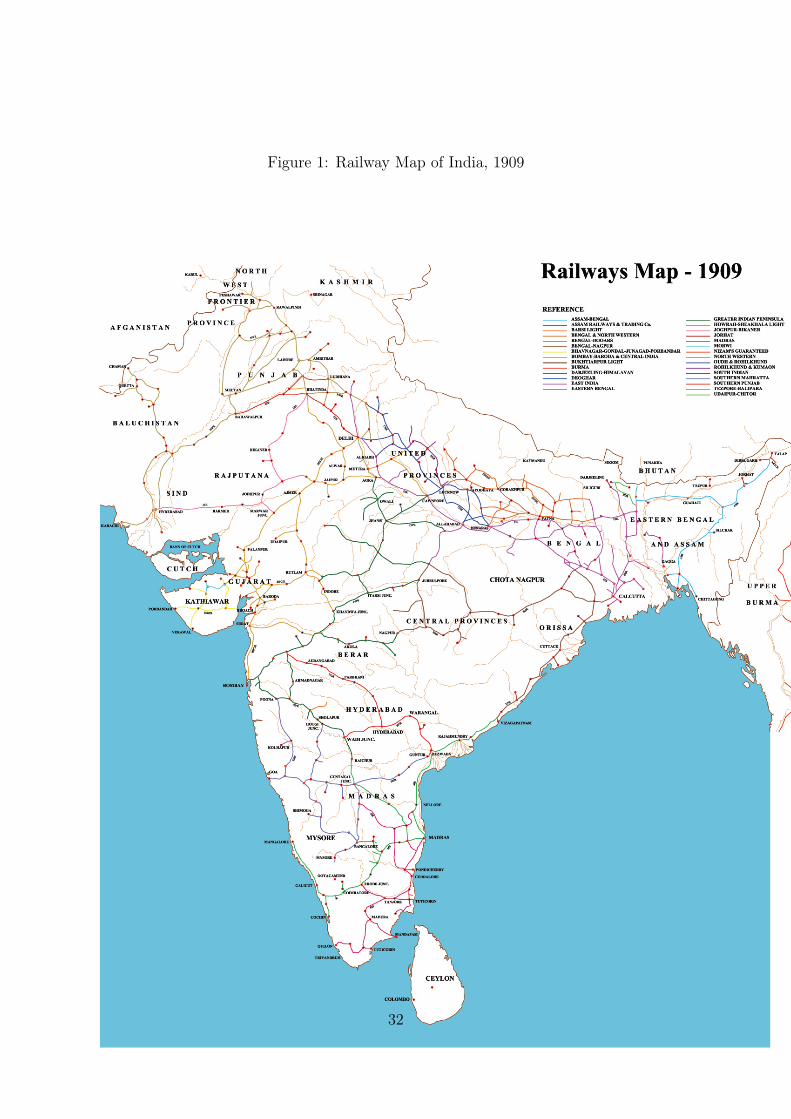
Figure 1: Railway Map of India, 1909

32

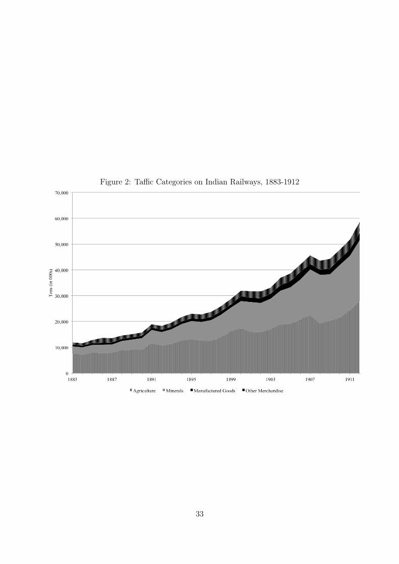
Figure 2: Taffic Categories on Indian Railways, 1883-1912

33

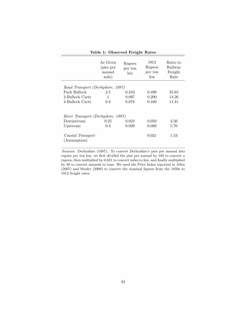
Table 1: Observed Freight Rates

As Given(pies permaundmile)

Rupeesper tonkm

1912Rupeesper tonkm

Ratio toRailwayFreightRate

Road Transport (Derbyshire, 1987)Pack Bullock 2.5 0.243 0.499 35.652-Bullock Carts 1 0.097 0.200 14.264-Bullock Carts 0.8 0.078 0.160 11.41

River Transport (Derbyshire, 1987)Downstream 0.25 0.024 0.050 3.56Upstream 0.4 0.039 0.080 5.70

Coastal Transport 0.021 1.53(Assumption)

Sources: Derbyshire (1987). To convert Derbyshire’s pies per maund intorupees per ton km, we first divided the pies per maund by 192 to convert orupees, then multiplied by 0.621 to convert miles to km, and finally multipliedby 30 to convert maunds to tons. We used the Price Index reported in Allen(2007) and Studer (2008) to convert the nominal figures from the 1850s to1912 freight rates.

34

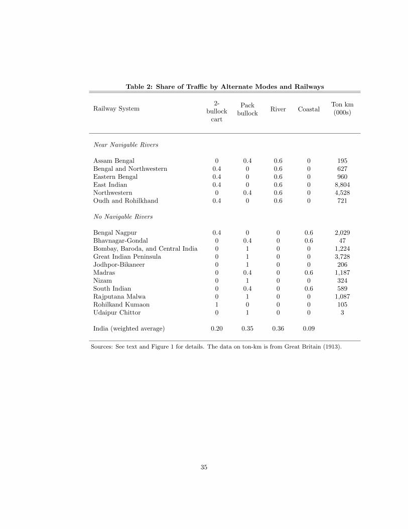
Table 2: Share of Traffic by Alternate Modes and Railways

Railway System2-

bullockcart

Packbullock

River CoastalTon km(000s)

Near Navigable Rivers

Assam Bengal 0 0.4 0.6 0 195Bengal and Northwestern 0.4 0 0.6 0 627Eastern Bengal 0.4 0 0.6 0 960East Indian 0.4 0 0.6 0 8,804Northwestern 0 0.4 0.6 0 4,528Oudh and Rohilkhand 0.4 0 0.6 0 721

No Navigable Rivers

Bengal Nagpur 0.4 0 0 0.6 2,029Bhavnagar-Gondal 0 0.4 0 0.6 47Bombay, Baroda, and Central India 0 1 0 0 1,224Great Indian Peninsula 0 1 0 0 3,728Jodhpor-Bikaneer 0 1 0 0 206Madras 0 0.4 0 0.6 1,187Nizam 0 1 0 0 324South Indian 0 0.4 0 0.6 589Rajputana Malwa 0 1 0 0 1,087Rohilkand Kumaon 1 0 0 0 105Udaipur Chittor 0 1 0 0 3

India (weighted average) 0.20 0.35 0.36 0.09

Sources: See text and Figure 1 for details. The data on ton-km is from Great Britain (1913).

35

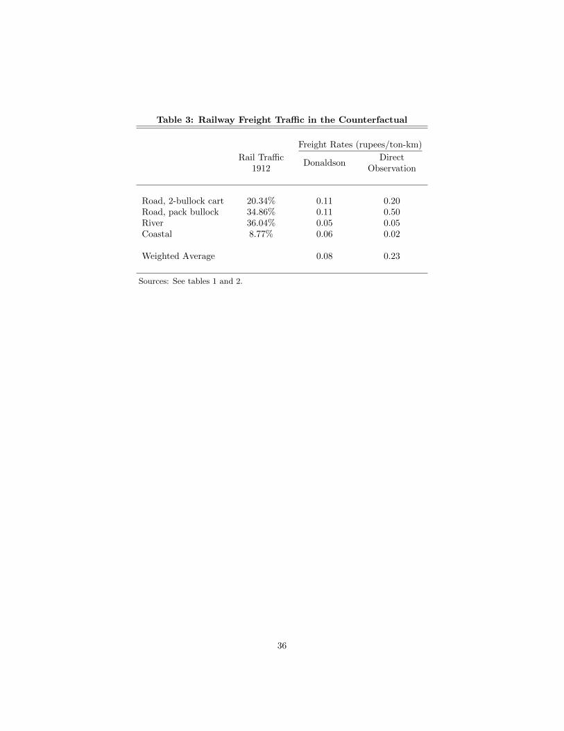
Table 3: Railway Freight Traffic in the Counterfactual

Freight Rates (rupees/ton-km)

Rail Traffic1912

DonaldsonDirect

Observation

Road, 2-bullock cart 20.34% 0.11 0.20Road, pack bullock 34.86% 0.11 0.50River 36.04% 0.05 0.05Coastal 8.77% 0.06 0.02

Weighted Average 0.08 0.23

Sources: See tables 1 and 2.

36

Table 4: Price Elasticity Estimates for Freight on Indian Railways

Dependent Variable: Ln (Freight Ton Miles)(1) (2) (3) (4)

Ln(Freight Rate) -0.9489** -0.7298*** -0.8384*** -0.6578***[0.3890] [0.1828] [0.1960] [0.1580]

Ln(Miles) 1.5246*** 0.9655*** 0.9690*** 1.1128***[0.1109] [0.0855] [0.0874] [0.0678]

Density (Train miles/Total Miles) 0.0003***[0.0001]

Year -0.0153** 0.0175***[0.0059] [0.0055]

Railway FE No Yes Yes YesYear FE No No Yes Yes

Observations 569 569 569 568

*** p<0.01, ** p<0.05, * p<0.1 Robust standard errors clustered at the railway-levelin brackets. The unit of analysis is railway-system*year from 1880 to 1912. SeeBogart and Chaudhary (2013) for details on the construction of the railway-level panel.

37

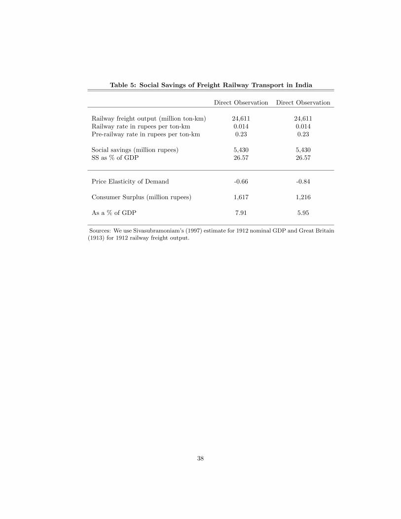
Table 5: Social Savings of Freight Railway Transport in India

Direct Observation Direct Observation

Railway freight output (million ton-km) 24,611 24,611Railway rate in rupees per ton-km 0.014 0.014Pre-railway rate in rupees per ton-km 0.23 0.23

Social savings (million rupees) 5,430 5,430SS as % of GDP 26.57 26.57

Price Elasticity of Demand -0.66 -0.84

Consumer Surplus (million rupees) 1,617 1,216

As a % of GDP 7.91 5.95

Sources: We use Sivasubramoniam’s (1997) estimate for 1912 nominal GDP and Great Britain(1913) for 1912 railway freight output.

38

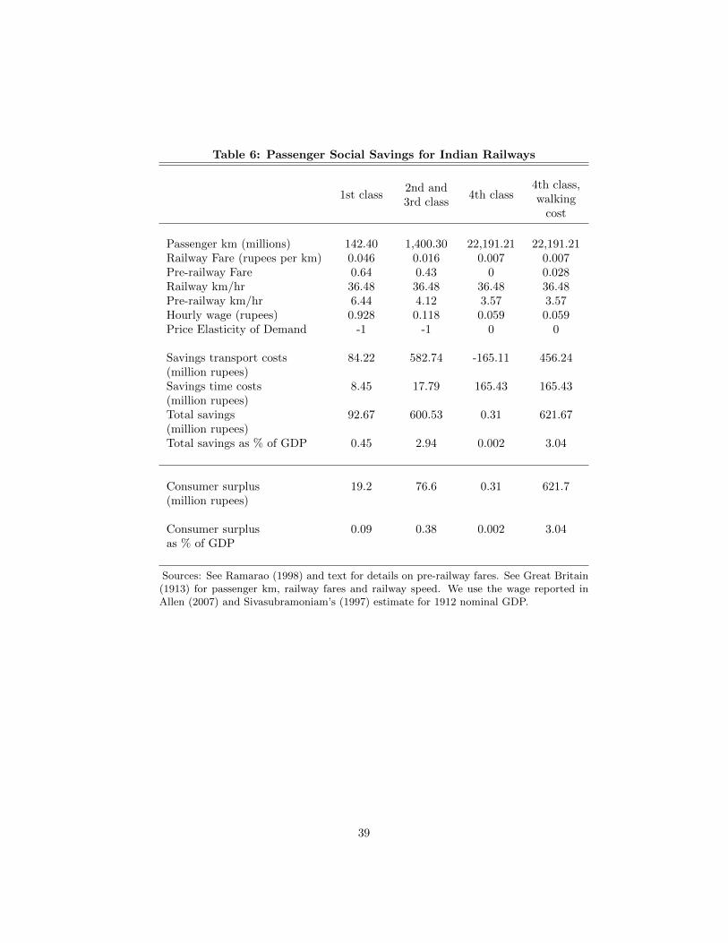
Table 6: Passenger Social Savings for Indian Railways

1st class2nd and3rd class

4th class4th class,walkingcost

Passenger km (millions) 142.40 1,400.30 22,191.21 22,191.21Railway Fare (rupees per km) 0.046 0.016 0.007 0.007Pre-railway Fare 0.64 0.43 0 0.028Railway km/hr 36.48 36.48 36.48 36.48Pre-railway km/hr 6.44 4.12 3.57 3.57Hourly wage (rupees) 0.928 0.118 0.059 0.059Price Elasticity of Demand -1 -1 0 0

Savings transport costs 84.22 582.74 -165.11 456.24(million rupees)Savings time costs 8.45 17.79 165.43 165.43(million rupees)Total savings 92.67 600.53 0.31 621.67(million rupees)Total savings as % of GDP 0.45 2.94 0.002 3.04

Consumer surplus 19.2 76.6 0.31 621.7(million rupees)

Consumer surplus 0.09 0.38 0.002 3.04as % of GDP

Sources: See Ramarao (1998) and text for details on pre-railway fares. See Great Britain(1913) for passenger km, railway fares and railway speed. We use the wage reported inAllen (2007) and Sivasubramoniam’s (1997) estimate for 1912 nominal GDP.

39

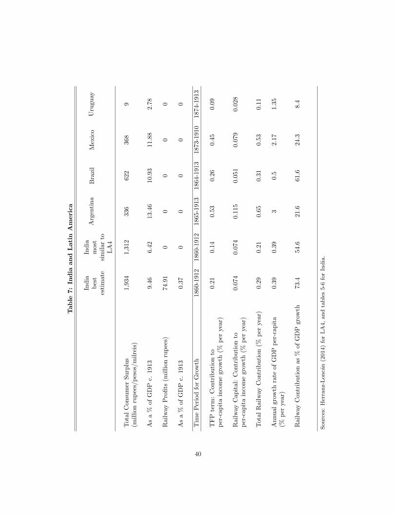
Table

7:In

dia

and

Latin

America

Ind

iab

est

esti

mate

Ind

iam

ost

sim

ilar

toL

A4

Arg

enti

na

Bra

zil

Mex

ico

Uru

gu

ay

Tot

alC

onsu

mer

Su

rplu

s1,9

34

1,3

12

336

622

368

9(m

illi

onru

pee

s/p

esos

/mil

reis

)

As

a%

ofG

DP

c.19

139.4

66.4

213.4

610

.93

11.8

82.7

8

Rai

lway

Pro

fits

(mil

lion

rup

ees)

74.9

10

00

00

As

a%

ofG

DP

c.19

130.3

70

00

00

Tim

eP

erio

dfo

rG

row

th1860-1

912

1860-1

912

1865-1

913

1864

-1913

1873-1

910

1874-1

913

TF

Pte

rm:

Con

trib

uti

onto

0.2

10.1

40.5

30.2

60.4

50.0

9p

er-c

apit

ain

com

egr

owth

(%p

erye

ar)

Rai

lway

Cap

ital

:C

ontr

ibu

tion

to0.0

74

0.0

74

0.1

15

0.051

0.0

79

0.0

28

per

-cap

ita

inco

me

grow

th(%

per

year

)

Tot

alR

ailw

ayC

ontr

ibu

tion

(%p

erye

ar)

0.2

90.2

10.6

50.3

10.5

30.1

1

An

nu

algr

owth

rate

ofG

DP

per

-cap

ita

0.3

90.3

93

0.5

2.1

71.3

5(%

per

yea

r)

Rai

lway

Con

trib

uti

onas

%of

GD

Pgr

owth

73.4

54.6

21.6

61.6

24.3

8.4

Sourc

es:

Her

ranz-

Lonca

n(2

014)

for

LA

4,

and

table

s5-6

for

India

.

40

Table

8:Decomposition

ofFre

ightand

PassengerSocialSavings

India

Argentina

Brazil

Mexico

Uruguay

Freight

Social

Savings

asa%

ofGDP

26.6

20.6

18.8

24.3

3.8

Additional

CSas

%of

GDP

5.95

11.61

8.97

11.48

2.19

(Pre-railway

freigh

trate/railway

rate)-1

16.01

5.66

6.47

9.48

2.66

FreightRailway

Revenues

as%

ofGDP

1.7

3.6

2.9

2.6

1.4

Passen

ger

Upper-class

SSas

%of

GDP

3.39

0.70

3.58

0.65

2.27

Low

er-class

SSas

%of

GDP

0.00

1.31

0.77

0.06

0.18

(nowalkingcosts)

Passen

ger,

Lower-class

PassengerRailway

Revenues

as%

ofGDP

0.81

0.61

0.47

0.40

0.53

Railway

Tim

eSavings

as%

ofGDP

0.81

1.92

1.25

0.46

0.70

(Railway

KMPH/P

reRailway

KMPH)-1

9.28

12.13

12.00

12.33

10.46

Fare/Hou

rlywage

0.13

0.05

0.06

0.13

0.12

Sourc

es:

Her

ranz-

Lonca

n(2

014)

for

LA

4,

and

table

s5-6

for

India

.

41

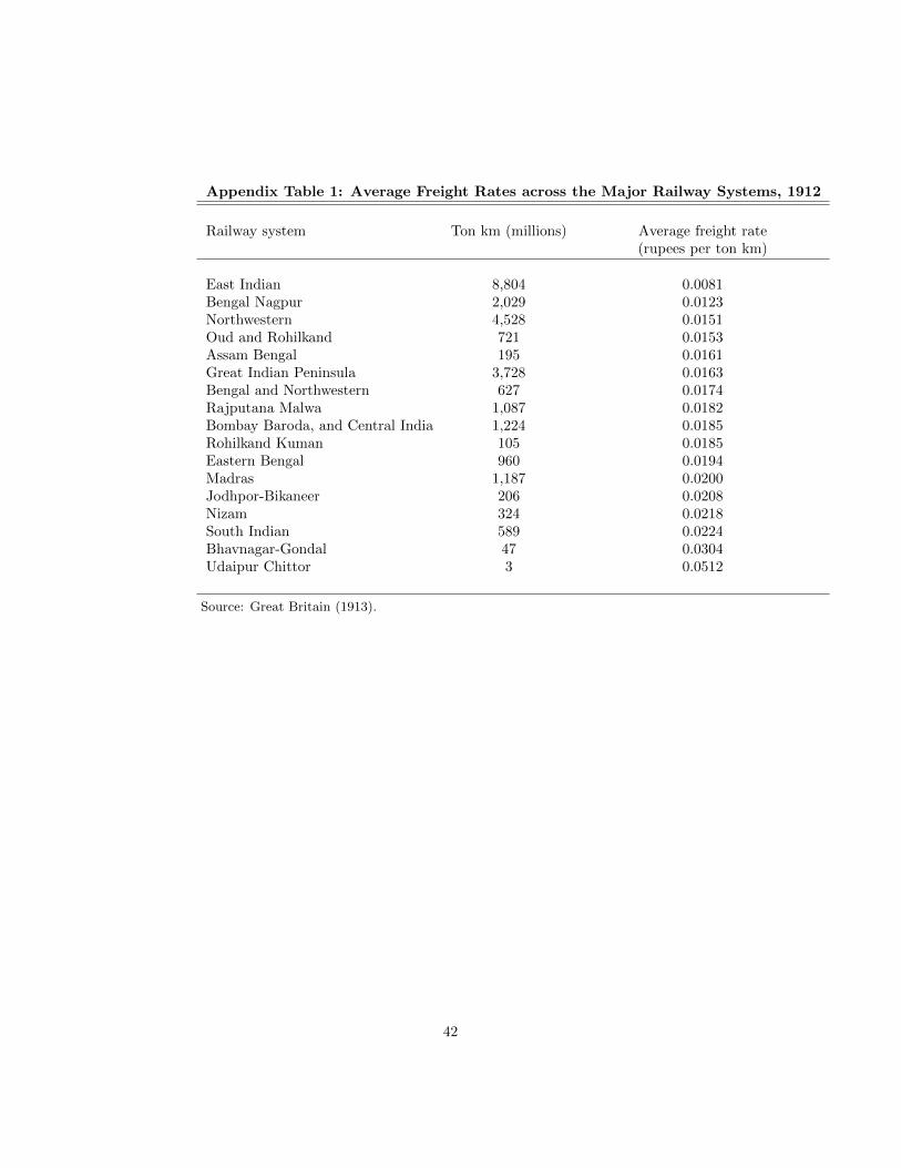
Appendix Table 1: Average Freight Rates across the Major Railway Systems, 1912

Railway system Ton km (millions) Average freight rate(rupees per ton km)

East Indian 8,804 0.0081Bengal Nagpur 2,029 0.0123Northwestern 4,528 0.0151Oud and Rohilkand 721 0.0153Assam Bengal 195 0.0161Great Indian Peninsula 3,728 0.0163Bengal and Northwestern 627 0.0174Rajputana Malwa 1,087 0.0182Bombay Baroda, and Central India 1,224 0.0185Rohilkand Kuman 105 0.0185Eastern Bengal 960 0.0194Madras 1,187 0.0200Jodhpor-Bikaneer 206 0.0208Nizam 324 0.0218South Indian 589 0.0224Bhavnagar-Gondal 47 0.0304Udaipur Chittor 3 0.0512

Source: Great Britain (1913).

42

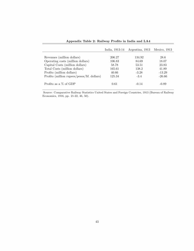
Appendix Table 2: Railway Profits in India and LA4

India, 1913-14 Argentina, 1913 Mexico, 1913

Revenues (million dollars) 206.27 134.92 28.6Operating costs (million dollars) 106.83 84.69 18.07Capital Costs (million dollars) 58.78 53.51 23.83Total Costs (million dollars) 165.61 138.2 41.89Profits (million dollars) 40.66 -3.28 -13.29Profits (million rupees/pesos/M. dollars) 125.34 -3.4 -26.66

Profits as a % of GDP 0.61 -0.14 -0.89

Source: Comparative Railway Statistics United States and Foreign Countries, 1913 (Bureau of RailwayEconomics, 1916, pp. 21-22, 46, 50).

43