The Gravity Approach for Trade Diversification in

Central AsiaMAENO Takaaki, Nihon University

Workshop on Economic development of New Silk Road26 – 27 August, 2011

Motivations• Two main motivations

– It is to reveal an important characteristics of trade structure for Central Asian countries that locate at the geographically middle of the new silk road.

– It is to clarify the impact of trade costs on trade flows for landlocked countries through measuring trade costs and estimating the determinants of them. And also, we will give some implications of economic development for countries on new silk road.

• We focus on the trade structure of Central Asian countries.

Outline

１． Introduction

２． Being Landlocked and Trade Cost

３． An Analysis of Trade Structure of Central Asia

４． Panel Data Analysis

５． Conclusion

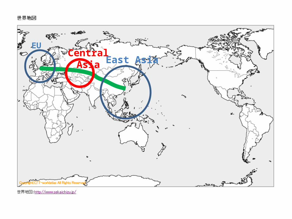
East AsiaEU

Central Asia

Central Asia (five countries)

the Caucasus region

１． Introduction• Since the late 1980s, MNEs in the developed

countries, including Japanese firms, expands their business overseas, and East Asian countries have achieved high economic growth through production process sharing.

• Decreasing Trade Costs– One of the main reasons for trade expansion in East Asia

is due to decreasing in trade costs

• What about the trade structure of Central Asian countries?

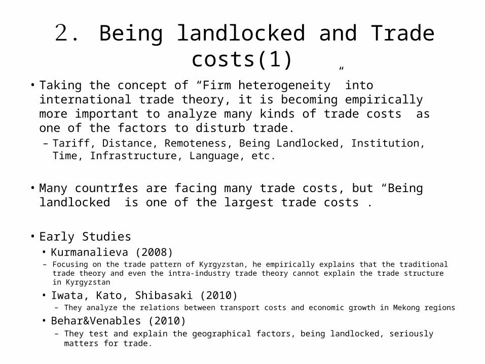
２． Being landlocked and Trade costs(1)

• Taking the concept of “Firm heterogeneity” into international trade theory, it is becoming empirically more important to analyze many kinds of trade costs as one of the factors to disturb trade.– Tariff, Distance, Remoteness, Being Landlocked, Institution, Time,

Infrastructure, Language, etc.

• Many countries are facing many trade costs, but “Being landlocked” is one of the largest trade costs .

• Early Studies• Kurmanalieva (2008)– Focusing on the trade pattern of Kyrgyzstan, he empirically explains that the traditional trade

theory and even the intra-industry trade theory cannot explain the trade structure in Kyrgyzstan

• Iwata, Kato, Shibasaki (2010)– They analyze the relations between transport costs and economic growth in Mekong regions

• Behar&Venables (2010)– They test and explain the geographical factors, being landlocked, seriously matters

for trade.

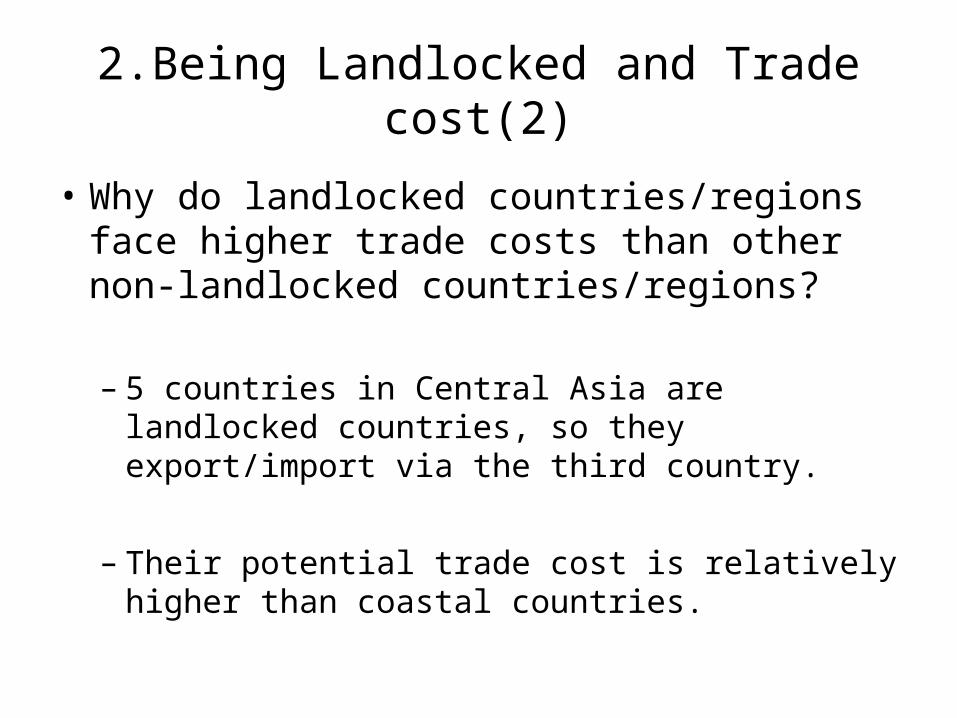
2.Being Landlocked and Trade cost(2)

• Why do landlocked countries/regions face higher trade costs than other non-landlocked countries/regions?

– 5 countries in Central Asia are landlocked countries, so they export/import via the third country.

– Their potential trade cost is relatively higher than coastal countries.

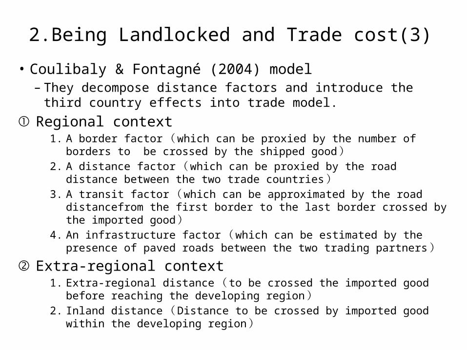
2.Being Landlocked and Trade cost(3)

• Coulibaly & Fontagné (2004) model– They decompose distance factors and introduce the third

country effects into trade model.

① Regional context1. A border factor （ which can be proxied by the number of borders

to be crossed by the shipped good ）2. A distance factor （ which can be proxied by the road distance

between the two trade countries ）3. A transit factor （ which can be approximated by the road

distancefrom the first border to the last border crossed by the imported good ）

4. An infrastructure factor （ which can be estimated by the presence of paved roads between the two trading partners ）

② Extra-regional context1. Extra-regional distance （ to be crossed the imported good

before reaching the developing region ）2. Inland distance （ Distance to be crossed by imported good

within the developing region ）

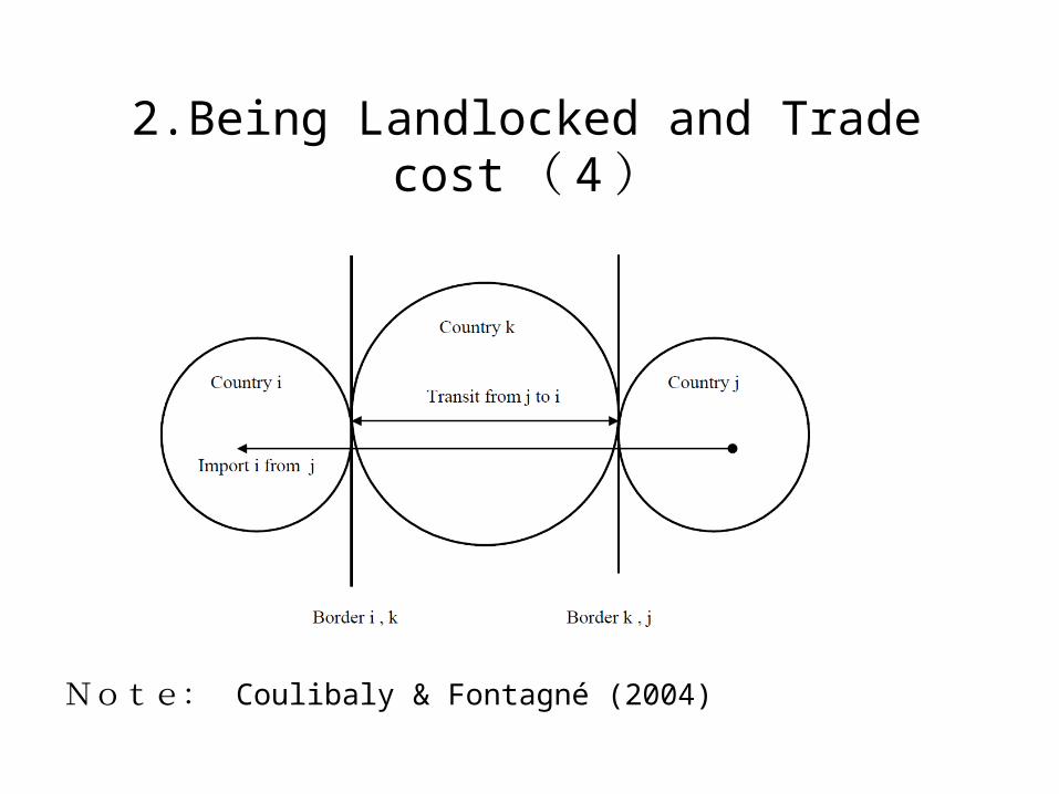
2.Being Landlocked and Trade cost （ 4 ）

Ｎｏｔｅ： Coulibaly & Fontagné (2004)

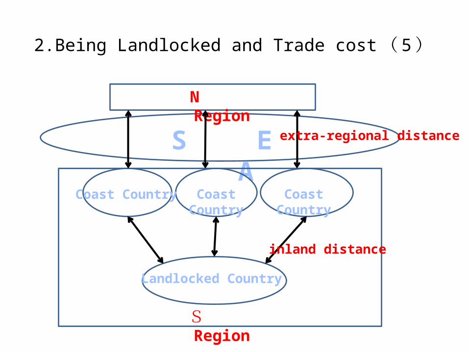
2.Being Landlocked and Trade cost （ 5 ）

S 　 E 　 A

N 　　　 Region

Ｓ　　　 Region

Coast Country Coast Country Coast Country

Landlocked Country

extra-regional distance

inland distance

３． An Analysis of Trade Structure of Central Asia （１）

• ＲＣＡ

• Export Similarity Index

• Trade Decomposition

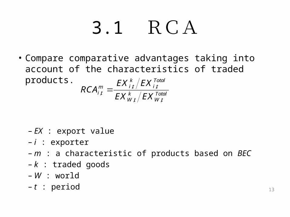
3.1 　ＲＣＡ• Compare comparative advantages taking into

account of the characteristics of traded products.

– EX : export value– i : exporter– m : a characteristic of products based on BEC– k : traded goods– W : world– t : period

TotaltW

ktW

Totalti

ktim

ti EXEX

EXEXRCA

,,

,,,

13

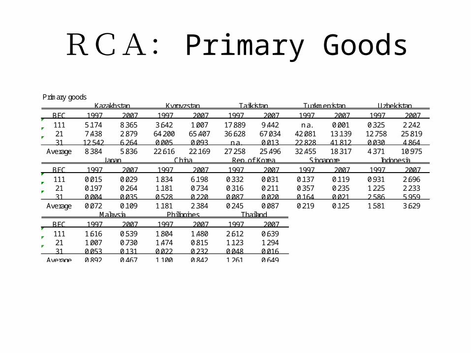
ＲＣＡ： Primary Goods

Primary goods

BEC 1997 2007 1997 2007 1997 2007 1997 2007 1997 2007111 5.174 8.365 3.642 1.007 17.889 9.442 n.a. 0.001 0.325 2.24221 7.438 2.879 64.200 65.407 36.628 67.034 42.081 13.139 12.758 25.81931 12.542 6.264 0.005 0.093 n.a. 0.013 22.828 41.812 0.030 4.864

Average 8.384 5.836 22.616 22.169 27.258 25.496 32.455 18.317 4.371 10.975

BEC 1997 2007 1997 2007 1997 2007 1997 2007 1997 2007111 0.015 0.029 1.834 6.198 0.332 0.031 0.137 0.119 0.931 2.69621 0.197 0.264 1.181 0.734 0.316 0.211 0.357 0.235 1.225 2.23331 0.004 0.035 0.528 0.220 0.087 0.020 0.164 0.021 2.586 5.959

Average 0.072 0.109 1.181 2.384 0.245 0.087 0.219 0.125 1.581 3.629

BEC 1997 2007 1997 2007 1997 2007111 1.616 0.539 1.804 1.480 2.612 0.63921 1.007 0.730 1.474 0.815 1.123 1.29431 0.053 0.131 0.022 0.232 0.048 0.016

Average 0.892 0.467 1.100 0.842 1.261 0.649

Kazakhstan Kyrgyzstan Tajikistan Turkmenistan Uzbekistan

J apan China Rep. of Korea Singapore Indonesia

Malaysia Philippines Thailand

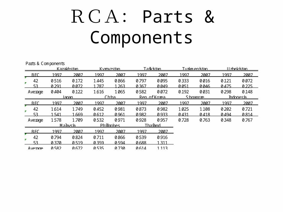
ＲＣＡ： Parts & Components

Parts & Components

BEC 1997 2007 1997 2007 1997 2007 1997 2007 1997 200742 0.516 0.172 1.445 0.866 0.797 0.095 0.333 0.016 0.121 0.07253 0.291 0.072 1.787 1.263 0.367 0.049 0.051 0.046 0.475 0.225

Average 0.404 0.122 1.616 1.065 0.582 0.072 0.192 0.031 0.298 0.148

BEC 1997 2007 1997 2007 1997 2007 1997 2007 1997 200742 1.614 1.749 0.452 0.981 0.873 0.982 1.025 1.108 0.202 0.72153 1.541 1.669 0.612 0.961 0.982 0.933 0.431 0.418 0.494 0.814

Average 1.578 1.709 0.532 0.971 0.928 0.957 0.728 0.763 0.348 0.767

BEC 1997 2007 1997 2007 1997 200742 0.794 0.824 0.711 0.866 0.539 0.91653 0.370 0.519 0.359 0.594 0.688 1.311

Average 0.582 0.672 0.535 0.730 0.614 1.113

Malaysia Philippines Thailand

Kazakhstan Kyrgyzstan Tajikistan Turkmenistan Uzbekistan

J apan China Rep. of Korea Singapore Indonesia

3.1 　ＲＣＡ（２）• East Asian countries have

comparative advantages in P&C that is relatively higher-value added.

• Central Asian countries have comparative advantage in primary good that is relatively low-value added.

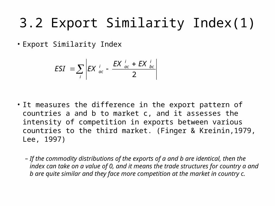
3.2 Export Similarity Index(1)

• Export Similarity Index

• It measures the difference in the export pattern of countries a and b to market c, and it assesses the intensity of competition in exports between various countries to the third market. (Finger & Kreinin,1979, Lee, 1997)

– If the commodity distributions of the exports of a and b are identical, then the index can take on a value of 0, and it means the trade structures for country a and b are quite similar and they face more competition at the market in country c.

i

ibc

iaci

ac

EXEXEXESI

2

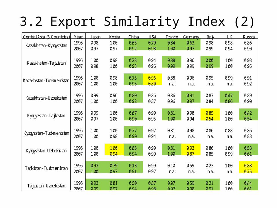
3.2 Export Similarity Index (2)Central Asia (5 Countries) Year J apan Korea China USA France Germany Italy UK Russia

1996 0.98 1.00 0.65 0.79 0.84 0.63 0.98 0.98 0.862007 0.97 0.97 0.92 0.98 1.00 0.97 0.99 0.94 0.90

1996 1.00 0.98 0.78 0.94 0.88 0.96 0.00 1.00 0.932007 0.98 1.00 0.98 0.96 0.99 0.99 0.99 1.00 0.95

1996 1.00 0.98 0.75 0.96 0.88 0.96 0.95 0.99 0.912007 1.00 1.00 0.95 0.80 n.a. n.a. n.a. n.a. 0.92

1996 0.99 0.96 0.80 0.86 0.86 0.91 0.87 0.47 0.892007 1.00 1.00 0.92 0.87 0.96 0.97 0.84 0.86 0.90

1996 0.99 1.00 0.67 0.99 0.81 0.98 0.85 1.00 0.422007 0.97 1.00 0.90 0.95 1.00 0.94 0.54 1.00 0.54

1996 1.00 1.00 0.77 0.97 0.81 0.98 0.86 0.88 0.862007 1.00 0.98 0.90 0.94 n.a. n.a. n.a. n.a. 0.83

1996 1.00 1.00 0.85 0.99 0.81 0.93 0.86 1.00 0.532007 1.00 0.94 0.94 0.99 1.00 0.87 0.85 0.99 0.61

1996 0.93 0.79 0.13 0.99 0.10 0.59 0.23 1.00 0.882007 1.00 0.97 0.91 0.97 n.a. n.a. n.a. n.a. 0.75

1996 0.93 0.81 0.50 0.87 0.07 0.59 0.21 1.00 0.442007 0.99 0.97 0.94 0.98 0.97 0.90 0.91 1.00 0.61

Kyrgyzstan- Uzbekistan

Tajikistan- Turkmenistan

Tajikistan- Uzbekistan

Kazakhstan- Kyrgyzstan

Kazakhstan- Tajikistan

Kazakhstan- Turkmenistan

Kazakhstan- Uzbekistan

Kyrgyzstan- Tajikistan

Kyrgyzstan- Turkmenistan

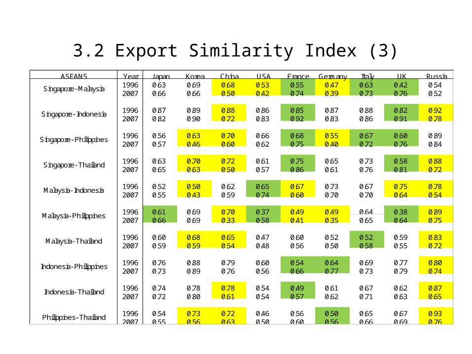
3.2 Export Similarity Index (3)ASEAN5 Year J apan Korea China USA France Germany Italy UK Russia

1996 0.63 0.69 0.68 0.53 0.55 0.47 0.63 0.42 0.542007 0.66 0.66 0.50 0.42 0.74 0.39 0.73 0.76 0.52

1996 0.87 0.89 0.88 0.86 0.85 0.87 0.88 0.82 0.922007 0.82 0.90 0.72 0.83 0.92 0.83 0.86 0.91 0.78

1996 0.56 0.63 0.70 0.66 0.68 0.55 0.67 0.60 0.892007 0.57 0.46 0.60 0.62 0.75 0.40 0.72 0.76 0.84

1996 0.63 0.70 0.72 0.61 0.75 0.65 0.73 0.58 0.882007 0.65 0.63 0.50 0.57 0.86 0.61 0.76 0.81 0.72

1996 0.52 0.50 0.62 0.65 0.67 0.73 0.67 0.75 0.782007 0.55 0.43 0.59 0.74 0.60 0.70 0.70 0.64 0.54

1996 0.61 0.69 0.70 0.37 0.49 0.49 0.64 0.38 0.892007 0.66 0.69 0.33 0.58 0.41 0.35 0.65 0.64 0.75

1996 0.60 0.68 0.65 0.47 0.60 0.52 0.52 0.59 0.832007 0.59 0.59 0.54 0.48 0.56 0.50 0.58 0.55 0.72

1996 0.76 0.88 0.79 0.60 0.54 0.64 0.69 0.77 0.802007 0.73 0.89 0.76 0.56 0.66 0.77 0.73 0.79 0.74

1996 0.74 0.78 0.78 0.54 0.49 0.61 0.67 0.62 0.872007 0.72 0.80 0.61 0.54 0.57 0.62 0.71 0.63 0.65

1996 0.54 0.73 0.72 0.46 0.56 0.50 0.65 0.67 0.932007 0.55 0.56 0.63 0.50 0.60 0.56 0.66 0.69 0.76

Singapore- Malaysia

Singapore- Indonesia

Singapore- Philippines

Singapore- Thailand

Malaysia- Indonesia

Malaysia- Philippines

Malaysia- Thailand

Indonesia- Philippines

Indonesia- Thailand

Philippines- Thailand

3.2 Export Similarity Index (4)• For ASEAN5, they face quite higher competition in

the U.S. and EU market in 1996, but they shift the market to East Asia.

• It is strongly associated with the development of production fragmentation in East Asia.

• Compared to ASEAN5, there is almost no international competition in the global market for Central Asian countries.

• Their industrial structures are different• They are relatively less advanced in industrial advances• They trade the different characteristics of products• They are facing higher trade costs

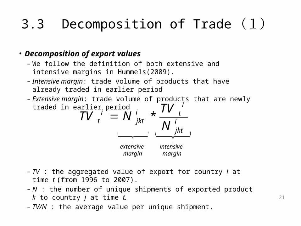
3.3 　 Decomposition of Trade （１）

• Decomposition of export values– We follow the definition of both extensive and intensive

margins in Hummels(2009).– Intensive margin: trade volume of products that have

already traded in earlier period– Extensive margin: trade volume of products that are newly

traded in earlier period

– TV : the aggregated value of export for country i at time t (from 1996 to 2007).

– N : the number of unique shipments of exported product k to country j at time t.

– TV/N : the average value per unique shipment.

ijkt

iti

jktit N

TVNTV *

intensive margin

extensive margin

21

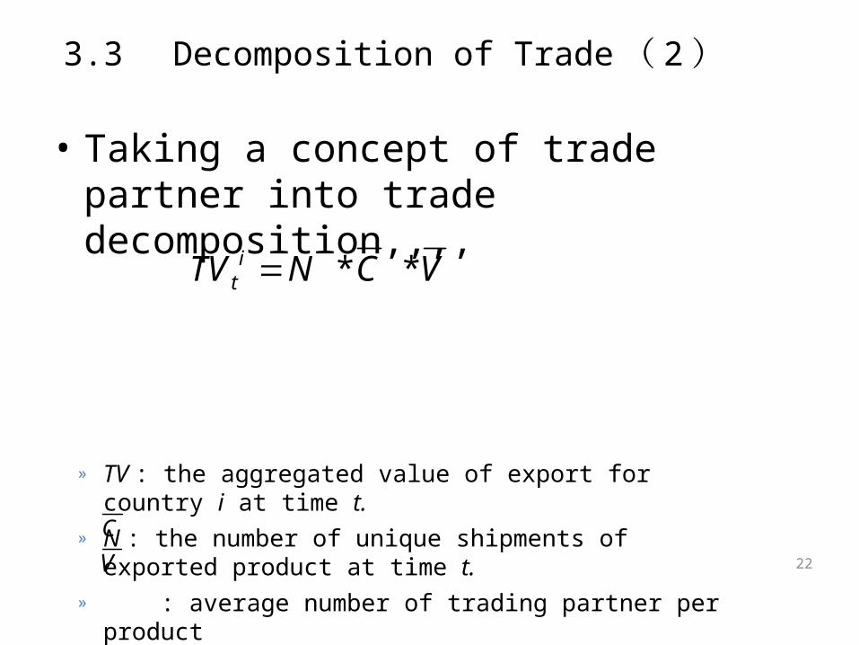
3.3 　 Decomposition of Trade （ 2 ）

• Taking a concept of trade partner into trade decomposition,,,,

» TV : the aggregated value of export for country i at time t.

» N : the number of unique shipments of exported product at time t.

» : average number of trading partner per product» : average export value per product-partner

C

V

VCNTV it **

22

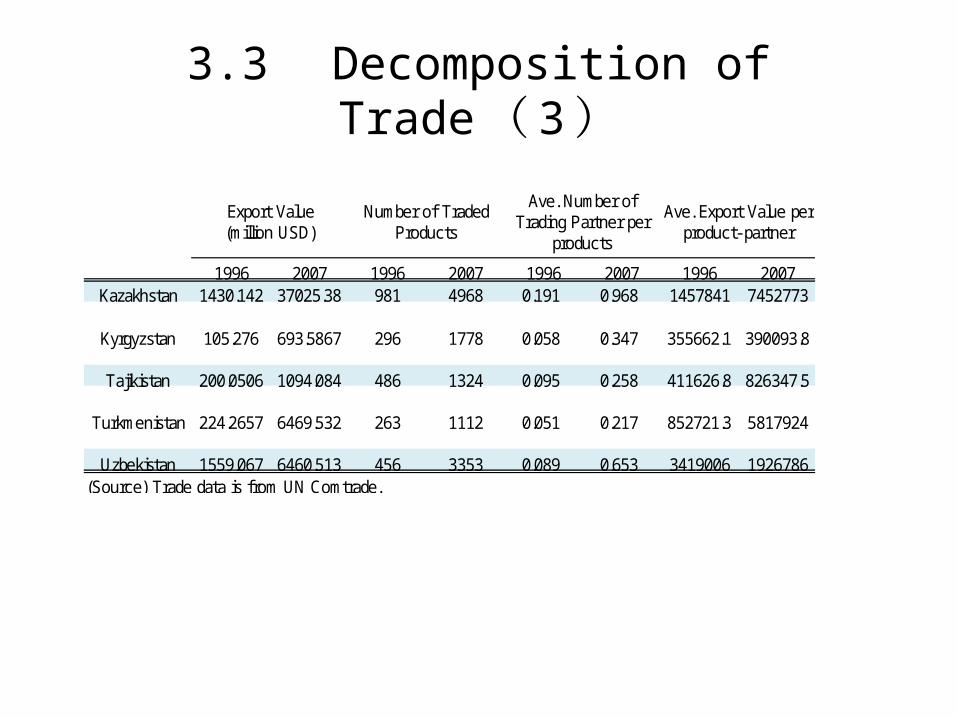
3.3 　 Decomposition of Trade （ 3 ）

1996 2007 1996 2007 1996 2007 1996 2007Kazakhstan 1430.142 37025.38 981 4968 0.191 0.968 1457841 7452773

Kyrgyzstan 105.276 693.5867 296 1778 0.058 0.347 355662.1 390093.8

Tajikistan 200.0506 1094.084 486 1324 0.095 0.258 411626.8 826347.5

Turkmenistan 224.2657 6469.532 263 1112 0.051 0.217 852721.3 5817924

Uzbekistan 1559.067 6460.513 456 3353 0.089 0.653 3419006 1926786(Source) Trade data is from UN Comtrade.

Ave. Number ofTrading Partner per

products

Ave. Export Value perproduct- partner

Export Value(million USD)

Number of TradedProducts

3.3 　 Decomposition of Trade （ 4 ）

• Their trade structure have been diversified at the aggregated level.

• The number of traded products and partners increases and also the export values per product and per partner increases.

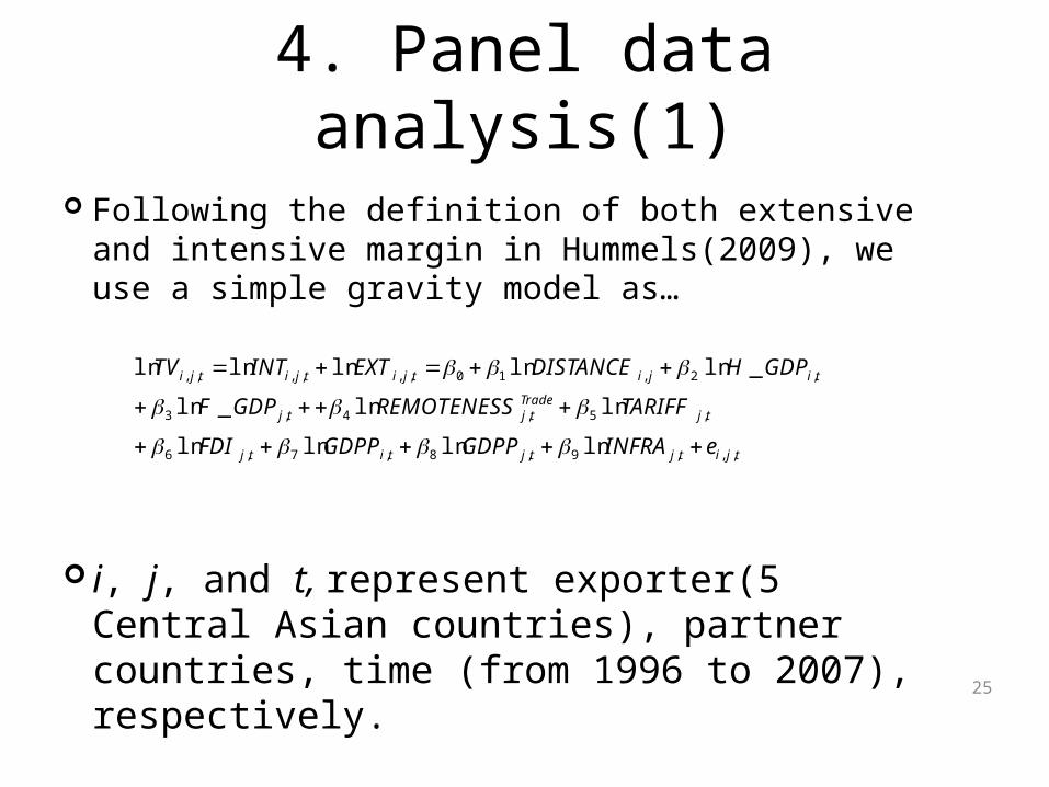
4. Panel data analysis(1)

Following the definition of both extensive and intensive margin in Hummels(2009), we use a simple gravity model as…

i, j, and t, represent exporter(5 Central Asian countries), partner countries, time (from 1996 to 2007), respectively.

tjitjtjtitj

tjTradetjtj

tijitjitjitji

eINFRAGDPPGDPPFDI

TARIFFREMOTENESSGDPF

GDPHDISTANCEEXTINTTV

,,,9,8,7,6

,5,4,3

,2,10,,,,,,

lnlnlnln

lnln_ln

_lnlnlnlnln

25

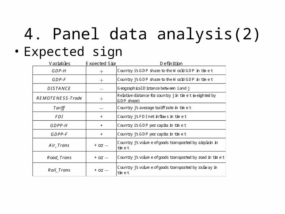
4. Panel data analysis(2)• Expected sign

Variables Expected Sign Definition

GDP-H ＋ Country i’s GDP share to the World GDP in time t

GDP-F ＋ Country j’s GDP share to the World GDP in time t

DISTANCE － Geographical Distance between i and j

REMOTENESS-Trade ＋Relative distance for country j in time t (weighted byGDP shere)

Tariff － Country j's average tariff rate in time t

FDI + Country j's FDI net inflows in time t

GDPP-H + Country i’s GDP per capita in time t

GDPP-F + Country j’s GDP per capita in time t

Air_Trans + or －Country j’s volume of goods transported by airplain intime t

Road_Trans + or － Country j’s volume of goods transported by road in time t

Rail_Trans + or －Country j’s volume of goods transported by railway intime t

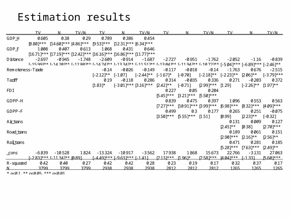
Estimation resultsTV N TV/ N TV N TV/ N TV N TV/ N TV N TV/ N

GDP_H 0.605 0.38 0.29 0.789 0.386 0.454[8.80]*** [14.60]*** [4.86]*** [9.53]*** [12.31]*** [6.34]***

GDP_F 1.008 0.407 0.613 1.068 0.431 0.646[16.71]*** [17.19]*** [12.42]*** [16.16]*** [16.86]*** [11.77]***

Distance - 2.697 - 0.945 - 1.748 - 2.609 - 0.914 - 1.687 - 2.727 - 0.951 - 1.762 - 2.052 - 1.16 - 0.839[- 15.99]***[- 14.20]***[- 12.80]***[- 14.74]***[- 13.34]***[- 11.51]***[- 13.04]***[- 11.94]***[- 10.72]***[- 5.04]*** [- 6.89]*** [- 2.46]**

Remoteness- Trade - 0.14 - 0.026 - 0.149 - 0.117 - 0.018 - 0.14 - 1.763 0.676 - 2.515[- 2.12]** [- 1.07] [- 2.44]** [- 1.67]* [- 0.70] [- 2.18]** [- 2.23]** [2.06]** [- 3.79]***

Tariff 0.19 - 0.118 0.286 0.314 - 0.035 0.336 0.271 - 0.203 0.372[1.83]* [- 3.01]*** [3.16]*** [2.42]** [- 0.71] [2.99]*** [1.29] [- 2.26]** [1.97]**

FDI 0.227 0.05 0.204[5.45]*** [3.21]*** [5.50]***

GDPP- H 0.839 0.475 0.397 1.096 0.553 0.563[7.27]*** [10.91]*** [3.99]*** [6.98]*** [8.32]*** [4.09]***

GDPP- F 0.499 0.3 0.177 0.265 0.251 - 0.075[3.50]*** [5.55]*** [1.51] [0.99] [2.23]** [- 0.32]

Air_trans 0.131 0.009 0.127[2.45]** [0.38] [2.70]***

Road_trans 0.189 0.061 0.151[2.90]*** [2.16]** [2.56]**

Rail_trans 0.471 0.281 0.185[5.28]*** [7.63]*** [2.49]**

_cons - 6.839 - 10.528 1.824 - 13.324 - 10.917 - 3.562 17.938 1.868 15.673 22.766 - 3.131 27.063[- 2.83]*** [- 11.34]***[0.89] [- 4.49]*** [- 9.63]*** [- 1.41] [7.13]*** [1.96]* [7.58]*** [4.04]*** [- 1.33] [5.60]***

R- squared 0.42 0.40 0.27 0.42 0.42 0.28 0.23 0.19 0.17 0.32 0.37 0.17N 3799 3799 3799 2938 2938 2938 2812 2812 2812 1265 1265 1265* p<0.1, ** p<0.05, *** p<0.01

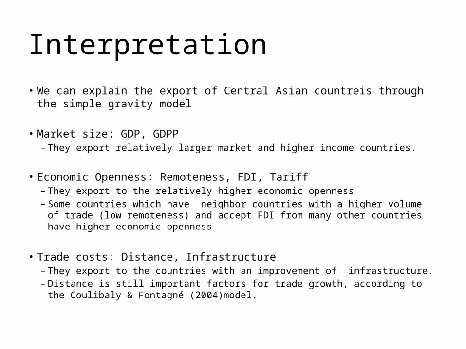
Interpretation• We can explain the export of Central Asian countreis through the simple gravity

model

• Market size: GDP, GDPP– They export relatively larger market and higher income countries.

• Economic Openness ： Remoteness, FDI, Tariff– They export to the relatively higher economic openness– Some countries which have neighbor countries with a higher volume of trade (low

remoteness) and accept FDI from many other countries have higher economic openness

• Trade costs ： Distance, Infrastructure– They export to the countries with an improvement of infrastructure.– Distance is still important factors for trade growth, according to the Coulibaly &

Fontagné (2004)model.

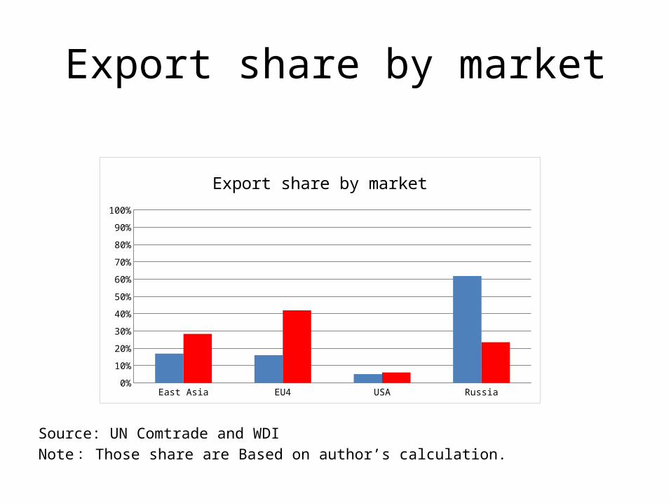
Export share by market

Source: UN Comtrade and WDINote ： Those share are Based on author’s calculation.

East Asia EU4 USA Russia

1996 0.169906234018865 0.160614774160664 0.0509279887238795 0.618551003096598

2007 0.283905454032114 0.419919069317739 0.0605789268179163 0.235596549832235

5%

15%

25%

35%

45%

55%

65%

75%

85%

95%

Export share by market

5. Ｃｏｎｃｌｕｓｉｏｎ s and future work

• Our studies show that the Central Asian countries have stronger comparative advantages for primary goods, but comparing to East Asian countries, they still face lower international competition.

• The gravity model can simply explain the trade diversification for the Central Asian countries.

• We clarify the negative relations between export and trade costs, especially infrastructure. So, it is important to decrease trade costs (ex. improve infrastructure) in order to trade growth and economic development.

• For the future work, we will measure and estimate some determinants of trade costs in order to lead the some implications to decrease trade costs and to achieve economic development for the related countries.

(source) World Bank

Cost to export (US$ per container)

Cost(US$) Rank Cost(US$) RankTajikistan 3000 191 Tajikistan 3150 192Kazakhstan 2730 189 Uzbekistan 3100 191Uzbekistan 2550 187 Kazakhstan 3005 190Kyrgyz Republic 2500 185 Kyrgyz Republic 3000 189

Cost to import (US$ per container)

Cost(US$) Rank Cost(US$) RankTajikistan 4500 193 Uzbekistan 4600 196Uzbekistan 4050 191 Tajikistan 4550 195Kazakhstan 2780 182 Kyrgyz Republic 3250 186Kyrgyz Republic 2450 176 Kazakhstan 3055 184

2006 2009

20092006

Reference• Tsuji, T., N.Ijiri, Y.Wu, M.Honda, and Y.Riku （2008），”Forming Beads-type Industrial Cities along New Silk Road”, CCAS

Working Paper Series No.009.• Anderson, J. and van, Wincoop,E. (2003), “Gravity with Gravitas: A solution to the Border Puzzle”, American Economic

Review, 93(1), pp. 170-192.• Behar, A. and A. Venables (2010), “Transport costs and International Trade”, University of Oxford, Department of

Economics Discussion Paper Series, Number 488.• Chaney, T. (2008), “Distorted Gravity: The Intensive and Extensive Margins of International Trade”, American Economic

Review, Vol. 98(4), pp. 1707-1721.• Coulibaly, S. and L. Fontagné (2004), “South-South Trade: Geography Matters”, CEPII Working Papers, No.2004-08.• Finger, J. M. & M. E. Kreinin (1979), “A measure of ‘export similarity’ and its possible use”, The Economic Journal, Vol. 89,

pp. 905-912.• Hummels, D. (2009), “Trends in Asian trade: implications for transport infrastructure and trade

costs”, in D. H. Brooks and D. Hummels(eds.), Infrastructure’s Role in Lowering Asia’s Trade Costs, ADB Institute and Edward Elgar Publishing.

• Iwata, Kato, Shibasaki (2010), “Impact of International Transportation Infrastructure Development on a Landlocked Country: Case Study in the Greater Mekong Subregion”, Proceedings of the 3 rd International Conference on Transportation and Logistics(T-LOG2010), CD-ROM, Fukuoka, Japan.

• Kurmanalieva, E. (2008), “Empirical Analysis of Kyrgyz Trade Patterns”, Eurasian Journal of Business and Economics, 1(1), pp. 83-97.

• Limao, N. and A. Venables (1999), “Infrastructure, Geographical Disadvantage, Transport Costs and Trade”, World Bank Policy Working Paper 2257.

• Shepherd & Wilson (2006), “Road Infrastructure in Europe and Central Asia: Does Network Quality Affect Trade?”, World Bank Policy Working Paper 4104.