Prepared for submission to JHEP

The Gravitational-Wave Physics

Rong-Gen Cai1,3 Zhoujian Cao2,4 Zong-Kuan Guo1,5 Shao-Jiang Wang1,3 Tao Yang1,3

1CAS Key Laboratory of Theoretical Physics, Institute of Theoretical Physics, Chinese Academyof Sciences, No.55 Zhong Guan Cun East Road, Beijing 100190, China

2Department of Astronomy, Beijing Normal University, No. 19, XinJieKouWai Street, Beijing100875, China

3School of Physical Sciences, University of Chinese Academy of Sciences, No.19A Yuquan Road,Beijing 100049, China

4Institute of Applied Mathematics, Academy of Mathematics and Systems Science, Chinese Academyof Sciences, No.55 Zhong Guan Cun East Road, Beijing 100190, China

5School of Astronomy and Space Science, University of Chinese Academy of Sciences, No.19AYuquan Road, Beijing 100049, China

E-mail: cairg@itp.ac.cn, zjcao@amt.ac.cn, guozk@itp.ac.cn,schwang@itp.ac.cn, yangtao@itp.ac.cn

Abstract: The direct detection of gravitational wave by Laser Interferometer Gravitational-Wave Observatory indicates the coming of the era of gravitational-wave astronomy andgravitational-wave cosmology. It is expected that more and more gravitational-wave eventswill be detected by currently existing and planned gravitational-wave detectors. The grav-itational waves open a new window to explore the Universe and various mysteries willbe disclosed through the gravitational-wave detection, combined with other cosmologicalprobes. The gravitational-wave physics is not only related to gravitation theory, but alsois closely tied to fundamental physics, cosmology and astrophysics. In this review article,three kinds of sources of gravitational waves and relevant physics will be discussed, namelygravitational waves produced during the inflation and preheating phases of the Universe,the gravitational waves produced during the first-order phase transition as the Universecools down and the gravitational waves from the three phases: inspiral, merger and ring-down of a compact binary system, respectively. We will also discuss the gravitational wavesas a standard siren to explore the evolution of the Universe.

Key words: gravitational waves, inflation, reheating, first order phase transition, binaryblack holes, standard siren

arX

iv:1

703.

0018

7v2

[gr

-qc]

27

May

201

7

Contents

1 Introduction 1

2 Gravitational Waves From Primordial Universe 32.1 During Inflation 42.2 During Preheating 62.3 Observational Implications 6

3 The Gravitational Waves From Phase Transitions 73.1 Bubble Nucleation 83.2 Bubble Expansion 93.3 Bubble Percolation 123.4 Gravitational Waves 14

4 The Gravitational Waves From Binary Systems 164.1 Post-Newtonian Approximation 184.2 Numerical Relativity 184.3 Black Hole Perturbation 214.4 Cosmological Probes 22

5 Conclusions 24

1 Introduction

On 11 February 2016, the LIGO Scientific Collaboration and the Virgo Collaboration [1]announced that on 14 September 2015 at 09:50:45 UTC the two detectors of the Laser In-terferometer Gravitational-Wave Observatory (LIGO) simultaneously observed a transientgravitational-wave (GW) signal. The GW event is named GW150914. The frequency ofthe signal increases from 35 to 250 Hz with a peak GW strain 1.0 × 10−21 at the 150 Hz.The GW signal is consistent with the one predicated by general relativity for the inspiraland merger of a pair of black hole and the ringdown of the resulting single black hole.The source is located at a luminosity distance of 410+160

−180 Mpc corresponding to a redshiftz = 0.09+0.03

−0.04. The initial black hole masses are 36+5−4M and 29+4

−4M and the resultingblack hole mass is 62+4

−4M. The mass difference 3.0+0.5−0.5M is radiated in the form of GWs.

This is the first direct detection of GW and the first observation of a binary black holemerger. On 15 June 2016, the second GW event, GW151226, was announced by the sameteam [2]. This time, observed signal lasts approximate 1 s, the frequency increases from35 to 450 Hz within 55 cycles, and the peak gravitational strain reaches 3.4+0.7

−0.9 × 10−22

at 450 Hz. The source is also the merger of two black holes with masses 14.2+8.3−3.7M· and

– 1 –

7.5+2.3−2.3M, respectively, the final black hole has mass 20.8+6.1

−1.7M. This event happenedwith a luminosity distance 440+180

−190 Mpc corresponding to a redshift 0.09+0.03−0.04.

The GW was predicted by Albert Einstein in 1916 [3, 4], 1 year later after he finallyformulated his theory on gravitation, genera relativity. But the physical reality of the GWsolution of the Einstein field equations was not showed until the Chapel Hill conference in1957 [5]. In [6, 7], it has been shown that GW carries energy and when passing throughthe spacetime in a form of a sandwich, it affects test particles. More than one century haspassed since the Einstein’s proposal of general relativity, although it passed various precisetests, some alternatives still survive, for example, scalar-tensor gravity theory, f(R) gravity,modified gravity with higher curvature terms, etc. On the other hand, based on generalrelativity, one has now a standard model (SM) of cosmology, ΛCDM model, which is quitewell consistent with various astronomical observations made so far. Now we understandwell that GW exists not only in general relativity, but also in other relativistic covariancegravity theories. Due to the limited space, this review is confined for the GWs in generalrelativity.

The sources of GWs could be classified into two categories roughly. One is called cos-mological origin, the other is relativistic astrophysical origin. In the cosmological case, GWscan be produced in the early stages of the Universe, for example, during the inflation andreheating epochs. Such GWs are called primordial GWs, and they will leave unique imprinton the cosmic microwave background (CMB), the so-called B-mode. On the other hand,during the evolution of the Universe, it is expected that various phase transitions (PTs)had happened as the temperature of the Universe decreases, for example, the symmetricbreaking of the grand unification theory, electroweak (EW) PT, quantum chromodynamics(QCD) PT, etc. During those PTs, GWs are also expected to be produced with differentfeatures. Also the interactions of topological defects such as cosmic string, domain wall,etc, produced during PTs, will create GWs. Therefore, the detection of GWs due to thosecosmological origins can reveal physics associated with the evolution of the Universe. In theastrophysics side, GWs can be produced in various processes, for example, rotation of non-symmetric neutron star, explosion of supernovae, inspiral, merger and ringdown of somecompact binaries including white dwarf, neutron star and/or black hole. In particular, thecompact binary systems are main sources for GW detection such as LIGO, Virgo, Kagra,Einstein Telescope, etc., ground-based GW experiments, and Laser Interferometer SpaceAntenna (LISA), Deci-Hertz Interferometer Gravitational wave Observatory (DECIGO),Big Bang Observer (BBO), Taiji, Tianqin, etc., space-based GW experiments.

Therefore, the GW physics is closely related to fundamental physics, cosmology andastrophysics. The direct detection of GWs in [1, 2] indicates the coming of the era of GWastronomy and GW cosmology. The detection of GWs opens a new window to explore theUniverse. Combining the electromagnetic (EM) radiation, neutrino, cosmic ray and GWs, itcould be expected that one is able to reveal various currently existing mysteries concerningthe early evolution of the Universe, property of dark matter, the nature of dark energy, etc.In this brief review, we are going to summarize some important aspects relevant to the GWphysics.

The outline of this review is as follows. Section 2 is going to introduce the GWs

– 2 –

produced in the primordial Universe and its detection through CMB. In particular, weemphasize the properties of GWs created during inflation and preheating processes andcurrent situation of detection of the primordial GWs. In section 3 we will discuss the GWsproduced during cosmic PT. There we will introduce the bubble nucleation, bubble expan-sion and bubble percolation. During the strong first-order PT, bubble collision, turbulentmagnetohydrodynamics (MHD) and sound wave are all the sources to produce GWs. Sec-tion 4 will mainly be devoted to discussions on the GWs from the dynamics of compactbinary systems. There we will introduce three main methods to solve the binary system:the post-Newtonian (PN) approximation, numerical relativity and the black hole perturba-tion, corresponding three phases: inspiral, merger and ringdown of two black holes system,respectively. In that section, we will also discuss the possibility of GWs produced by binarysystems as a cosmological probe. With this new probe, it is expected to have a strongconstraint on cosmological parameters, combining with other cosmological probes.

2 Gravitational Waves From Primordial Universe

In order to solve some problems in big-bang cosmology such as the horizon and flatnessproblems, inflationary scenario was introduced [8–10], in which a period of accelerated ex-pansion of the Universe happened at early times. Inflation not only predicts the primordialscalar perturbations, which provide a natural way to generating the anisotropies of theCMB radiation and the initial tiny seeds of the large-scale structure observed today in theUniverse, but also generates a stochastic background of the primordial GWs. Although sucha stochastic background of the primordial GWs has not been observed yet, its detectionwould open a new window to understanding the physics of the early Universe and thus theorigin and evolution of the Universe. In this section, we shall firstly review the properties ofthe primordial GWs produced during inflation and preheating (see Fig. 1), and then discussobservational implications.

GWs are described by a transverse-traceless gauge-invariant tensor perturbation, hij ,in a Friedman-Robertson-Walker (FRW) metric,

ds2 = a2(τ)[−dτ2 + (δij + hij)dx

idxj], (2.1)

where τ is the conformal time and a is the scale factor, and hij satisfies ∂ihij = 0 andδijhij = 0. To first order in hij , the perturbed Einstein equation reads

h′′ij + 2Hh′ij − O2hij =2

M2pl

ΠTTij , (2.2)

where the prime denotes the derivative with respect to τ , H ≡ a′/a is the Hubble parameterin τ , Mpl ≡ (8πG)−1/2 is the reduced Planck mass, and the source term; ΠTT

ij is thetransverse-traceless projection of the anisotropic stress tensor Tij . Since hij is symmetric,transverse and trace-free, tensor modes are left with two physical degrees of freedom, whichare expanded in the Fourier space as

hij(τ,x) =

∫d3k

(2π)3/2eik·x

[h+k (τ)e+ij(x) + h×k (τ)e×ij(x)

], (2.3)

– 3 –

inflation reheating

V(ϕ)

ϕ

Figure 1. The schematic illustration of the inflaton potential. In the slow-roll inflationary scenario,an accelerated expansion of the Universe occurs when the inflaton rolls slowly along its potential.After inflation ends, the inflaton oscillates around the minimum of its potential, whose energy isconverted into radiations.

where e+,×ij are the polarization tensors with two polarization states (+,×) of GWs. Wehave the power spectrum of GWs as

PT (τ, k) =k3

2π2(|h+k |

2 + |h×k |2), (2.4)

and the energy spectrum of GWs as Ωgw(τ, k) ≡ dρgw/d ln k/ρc, where

ρgw(τ, k) =1

4a2M2

pl〈h′ijh′ij〉 (2.5)

is the energy density and ρc = 3H2M2pl is the critical density of the Universe.

2.1 During Inflation

In the standard single-field slow-roll inflationary scenario, at first order in perturbationtheory Eq. (2.2) reduces to a free wave equation. In this case, the wave equation cananalytically be solved in the slow-roll approximation. The Bunch-Davies vacuum conditionin the asymptotic past is imposed because the modes lie well inside the Hubble radius. Ofcourse, if a general vacuum condition is imposed, there are additional features in the powerspectrum. During inflation, quantum fluctuations are amplified and stretched, and thennearly frozen on super-Hubble scales. The single-field slow-roll inflation predicts a slightlyred-tilted spectrum:

PT (k) =8

M2pl

(H

2π

)2

, (2.6)

– 4 –

and a consistency relation nT = −r/8 between the tensor spectral index nT and the tensor-to-scalar ratio r. Here, nT and r are evaluated at the epoch when a given perturbation modeleaves the Hubble horizon, i.e. k = aH. We usually introduce the tensor-to-scalar ratior ≡ AT /AS at a pivot scale k∗, i.e. the amplitude of tensor perturbations AT with respectto that of scalar perturbations AS . The red-tilted spectrum means that the amplitude oftensor perturbations becomes small on small scales due to the fact that large-scale modesare earlier stretched across the Hubble horizon than small-scale modes as the energy densityslowly decreases during inflation. From the wave equation we see that the evolution of hijdepends explicitly on a(τ) and implicitly on inflation potential through FRW equations.Hence the power spectrum of GWs encodes useful information on the evolution of the scalefactor. Moreover, the tensor-to-scalar ratio is related to the energy scale of inflation byV = 3π2M4

plAsr/2 = (1.88× 1016GeV)4r/0.10. Here we have adopted the estimated valueof the amplitude of scalar perturbations from the Planck 2015 data [11]. Different modelspredict different values of the tensor-to-scalar ratio. For example, the simplest chaoticinflation with a quartic potential [10] predicts a large value of r ≈ 0.26 while the R2

inflation [12] predicts a small value of r ≈ 0.0033 to lowest order in slow-roll parameters ifthe number of e-folds N∗ = 60 is assumed. With the help of the scalar spectral index, theestimated value of r is robust to discriminate slow-roll inflationary models. In summary,the measurement of the power spectrum of GWs helps us to

• test the vacuum initial condition,

• detect the evolution of the scale factor,

• determine the energy scale of inflation,

• discriminate inflationary models.

If the primordial GWs are detected, the next important question to answer is whatis the shape of the power spectrum of GWs and whether there are additional features inthe power spectrum. In the slow-roll inflationary scenario, the shape of the tensor powerspectrum is characterized by the tensor spectral index nT since the running of the spectralindex is negligible to the lowest order in slow-roll parameters. More general shapes beyondslow-roll may be reconstructed by using a binning method of a cubic spline interpolationin a logarithmic wavenumber space [13–15]. Checking the consistency relation betweennT and r provides a powerful test of the single-field slow-roll inflationary scenario. Theviolation of the consistency relation could in principle come from the following two aspects.The first is that the second and third terms on the left hand side of Eq. (2.2) are modifiedin general inflationary models, such as the k-inflation [16], Gauss-Bonnet inflation [17–19] and generalized G-inflation [20]. In the model of k-inflation, the consistency relationbecomes nT = −r/8cS , where cS is the sound speed of scalar perturbations. In the Gauss-Bonnet inflationary model, the consistency relation is broken due to nT = −r/8 − δ1,where δ1 is determined by the Gauss-Bonnet coupling term. In the model of generalizedG-inflation, the tensor spectral index not only depends on the evolution of the scale factorbut also the higher-order derivative terms, which admits a blue-tilted power spectrum of

– 5 –

GWs. The second is that there exists a non-negligible source term on the right hand side ofEq. (2.2) during inflation. In this case, the wave equation is solved by the Green’s functionmethod. Possible sources of generating GWs include first-order scalar perturbations [21],perturbations of the extra field such as the curvaton [22] and spectator field [23, 24], andparticle production during inflation [25].

2.2 During Preheating

In the inflationary scenario, at the end of inflation, the inflaton field begins to oscillatearound the minimum of its potential. Such coherent oscillations produce elementary parti-cles and eventually reheat the Universe. This process is called reheating [26]. The couplingbetween the inflaton field and other fields is necessarily tiny ensuring that reheating proceedsslowly. Preheating provides a more rapidly efficient mechanism for extracting energy fromthe inflation field by parametric resonance [27]. Such a process is so rapid that the producedparticles are not in thermal equilibrium. The preheating leads to large and time-dependentinhomogeneities of the stress tensor that source a stochastic background of GWs [28]. Un-like GWs produced during inflation, they are generated and remain in the Hubble horizonuntil now. Clearly, their wavelengths are smaller than the Hubble radius at the time ofGW production. Therefore, the peak frequency of this type of stochastic GWs is typicallyof order more than 103 Hz. Detecting such high-frequency GWs is particularly challenging.For example, for the φ4 and φ2 chaotic inflationary models, lattice simulations [29] showthat preheating can lead to GWs with frequencies of around 106 ∼ 108 Hz and peak powerof Ωgwh

2 ≈ 10−9 ∼ 10−11 at present [30]. For hybrid inflation, GWs cover a larger rangeof frequencies. The peak wavelength depends essentially on the coupling constant [31].See [32] for the most recent review on the GWs from the inflationary era and preheatingera.

2.3 Observational Implications

Observational constraints on GWs produced during inflation mainly come from the B-modepolarization of the CMB anisotropies. Such GWs generate a quadrupolar anisotropy ofmomentumm = 2 in the intensity field of photons at the epoch of recombination while scalarperturbations generate only a quadrupolar anisotropy of momentum m = 0. Importantly,only the quadrupolar anisotropy of momentum m = 2 causes the B-mode polarization.Therefore, the measurement of the B-mode polarization allows us to probe GWs producedduring inflation. The Planck 2015 data give the 95% confidence level upper bound forthe tensor-to-scalar ratio r0.002 < 0.10 at the pivot scale k∗ = 0.002 Mpc−1 [11], which isimproved to r0.002 < 0.08 by adding the BKP cross-correlation likelihood [33]. With the helpof the scalar spectral index nS , slow-roll inflationary models are discriminated in the r−nSplane, as shown in Fig. 2. For example, the inflationary model with a quartic potential [10]is strongly disfavored by recent CMB data. Future ground-based and space-based CMBexperiments will provide high precision measurements of the B-mode polarization. Actually,constraints on GWs produced during inflation from measurements of the CMB anisotropiesare limited to a narrow scale range of 10−4 ∼ 10−1 Mpc−1, which corresponds to the changeof e-folds number ∆N ≈ 8. This implies that it is impossible to detect the global shape

– 6 –

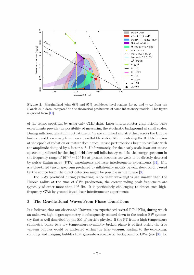
Figure 2. Marginalized joint 68% and 95% confidence level regions for ns and r0.002 from thePlanck 2015 data, compared to the theoretical predictions of some inflationary models. This figureis quoted from [11].

of the tensor spectrum by using only CMB data. Laser interferometer gravitational-waveexperiments provide the possibility of measuring the stochastic background at small scales.During inflation, quantum fluctuations of hij are amplified and stretched across the Hubblehorizon, and then nearly frozen on super-Hubble scales. After reentering the Hubble horizonat the epoch of radiation or matter dominance, tensor perturbations begin to oscillate withthe amplitude damped by a factor a−1. Unfortunately, for the nearly scale-invariant tensorspectrum predicted by the single-field slow-roll inflationary models, the energy spectrum inthe frequency range of 10−10 ∼ 103 Hz at present becomes too weak to be directly detectedby pulsar timing array (PTA) experiments and laser interferometer experiments [34]. If itis a blue-tilted tensor spectrum predicted by inflationary models beyond slow-roll or causedby the source term, the direct detection might be possible in the future [35].

For GWs produced during preheating, since their wavelengths are smaller than theHubble radius at the time of GWs production, the corresponding peak frequencies aretypically of order more than 103 Hz. It is particularly challenging to detect such high-frequency GWs by ground-based laser interferometer experiments.

3 The Gravitational Waves From Phase Transitions

It is believed that our observable Universe has experienced several PTs (PTs), during whichan unknown high-degree symmetry is subsequently relaxed down to the broken EW symme-try that is well described by the SM of particle physics. If the PT from a high-temperaturesymmetric phase to a low-temperature symmetry-broken phase is of first order, the truevacuum bubbles would be nucleated within the false vacuum, leading to the expanding,colliding and merging bubbles that generate a stochastic background of GWs (see [36] for

– 7 –

recent review and [37] for the discussions of GWs from cosmic strings and domain walls,which will not be discussed in this review). The primary motivations to study the GWsfrom PTs are two-folds: First, the EWPT of SM is cross-over according to the current mea-surements of Higgs mass. Therefore, any detections of GWs from PTs would necessarilyprovide us a unique probe beyond the SM, which cannot be directly probed by the particlecolliders in a foreseeable future; second, the stochastic backgrounds of GWs also consist ofthe GWs from the inflation era and the reheating era and the other cosmological defeatsfrom PTs like cosmic strings and domain walls. Therefore, it would help us to extract theGWs of astrophysical sources from the stochastic backgrounds of GWs. However, the topicsof detections are not discussed in this review, which should merit another paper to discusshow to detect the stochastic background of GWs and how to distinguish the signals of PTsfrom those signals of reheating or other cosmological defeats.

3.1 Bubble Nucleation

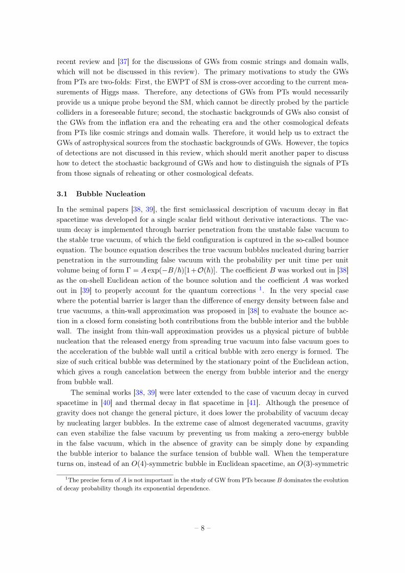
In the seminal papers [38, 39], the first semiclassical description of vacuum decay in flatspacetime was developed for a single scalar field without derivative interactions. The vac-uum decay is implemented through barrier penetration from the unstable false vacuum tothe stable true vacuum, of which the field configuration is captured in the so-called bounceequation. The bounce equation describes the true vacuum bubbles nucleated during barrierpenetration in the surrounding false vacuum with the probability per unit time per unitvolume being of form Γ = A exp(−B/~)[1+O(~)]. The coefficient B was worked out in [38]as the on-shell Euclidean action of the bounce solution and the coefficient A was workedout in [39] to properly account for the quantum corrections 1. In the very special casewhere the potential barrier is larger than the difference of energy density between false andtrue vacuums, a thin-wall approximation was proposed in [38] to evaluate the bounce ac-tion in a closed form consisting both contributions from the bubble interior and the bubblewall. The insight from thin-wall approximation provides us a physical picture of bubblenucleation that the released energy from spreading true vacuum into false vacuum goes tothe acceleration of the bubble wall until a critical bubble with zero energy is formed. Thesize of such critical bubble was determined by the stationary point of the Euclidean action,which gives a rough cancelation between the energy from bubble interior and the energyfrom bubble wall.

The seminal works [38, 39] were later extended to the case of vacuum decay in curvedspacetime in [40] and thermal decay in flat spacetime in [41]. Although the presence ofgravity does not change the general picture, it does lower the probability of vacuum decayby nucleating larger bubbles. In the extreme case of almost degenerated vacuums, gravitycan even stabilize the false vacuum by preventing us from making a zero-energy bubblein the false vacuum, which in the absence of gravity can be simply done by expandingthe bubble interior to balance the surface tension of bubble wall. When the temperatureturns on, instead of an O(4)-symmetric bubble in Euclidean spacetime, an O(3)-symmetric

1The precise form of A is not important in the study of GW from PTs because B dominates the evolutionof decay probability though its exponential dependence.

– 8 –

bubble solution that is periodic in time direction with period of inverse temperature T−1 isexpected, and the size of such critical bubble is determined by the maximum point of totalenergy. The tunneling rate was estimated in [41, 42] as

Γ(T ) ' T 4

(S3[φB(r), T ]

2πT

) 32

exp

(−S3[φB(r), T ]

T

), (3.1)

where the Euclidean action S3[φ(r), T ],

S3[φ(r)] = 4π

∫ ∞0

drr2

[1

2

(dφ

dr

)2

+ V (φ, T )

], (3.2)

is estimated at the bounce profile φB(r) of equation-of-motion,

d2φ

dr2+

2

r

dφ

dr=∂V

∂φ. (3.3)

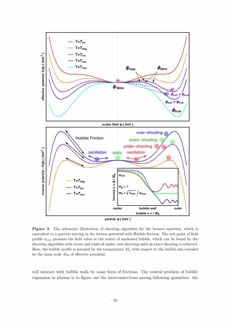
The effective potential usually consists of tree-level potential, zero-temperature correctionsand finite-temperature corrections including the daisy resummation. Recently, a new ther-mal resummation procedure was proposed in [43], which makes it possible to match theoriesto an EFT at finite temperature. Future works can be carried out along this direction. Thenaive strategy of solving above bounce equation is the shooting algorithm, which is illus-trated in Fig. 3. When multiple fields are involved at play, four approaches were introducedin the literatures, the early trial [44], the undamping/damping algorithm [45], the wildlyadopted path deformation algorithm [46], and the recently proposed semi-analytic pertur-bative approach [47].

The generalization of [38] in the case of non-zero cosmological constant allowed forboth false and true vacuums was carried out in [48]. The vacuum decay is enhanced inthe presence of gravity when the average of two vacuums is positive and suppressed whenboth vacuums are negative. The vacuum decay for a positive false vacuum but negativeaverage of two vacuums is enhanced or suppressed when the gravitational effect becomesimportant or not. There is currently no satisfactory description of thermal decay in curvedspacetime; however, we will clarify in the future work that the gravity correction only scalesas κ/(TR3), and it is not important because the characteristic size of bubble R is muchlarger than the Planck length

√κ ∼ 1/

√G for the characteristic scale of PT below the

Planck scale.

3.2 Bubble Expansion

After the bubble is nucleated within false vacuum, the bubble wall will rapidly expanduntil approaching the speed of light [38] or colliding with other bubble walls. However,the realistic background is actually a thermal plasma full of relativistic particles 2, which

2In this review, we are only interested in the GWs from PTs that happened in radiation dominatedera. For GWs from PTs that happened in inflation era and matter dominated era, please refer to [49–51]and [52], respectively. See also [53] for non-standard cosmology with an additional new component thatredshifts faster than radiation.

– 9 –

T=Tinf

T=Tdeg

T=Ttra

T=Tnuc

T=Tvan

ϕexit = ϕtrue

ϕzeroϕmax

ϕexit < ϕtrue

ϕ false

ϕtrue

scalar field ϕ [ GeV ]

effectivepotentialV(ϕ

)[GeV

4]

T=Tdeg

T=Ttra

T=Tnuc

over-shooting

exact-shooting

under-shooting

oscillation static

Hubble Friction

ϕexit

Mϕ = T

MR = Vmax ϕmax

center bubble wall outer

bubble x = r MR

bouncey=ϕ

/M

ϕ

oscillation

particle ϕ [ GeV ]

inversepotential

-V(ϕ

)[GeV

4]

Figure 3. The schematic illustration of shooting algorithm for the bounce equation, which isequivalent to a particle moving in the inverse potential with Hubble friction. The exit point of fieldprofile φexit presents the field value at the center of nucleated bubble, which can be found by theshooting algorithm with errors and trials of under/over shooting until an exact shooting is achieved.Here, the bubble profile is rescaled by the temperature Mφ with respect to the bubble size rescaledby the mass scale MR of effective potential.

will interact with bubble walls by some form of frictions. The central problem of bubbleexpansion in plasma is to figure out the interconnections among following quantities: the

– 10 –

bubble wall velocity vw, the friction η on the wall from plasma, the strength α of PT thatmeasure the released vacuum energy density with respect to the radiation energy density,and the efficiency factors κφ and κv that measure the capability of transferring the liberatedvacuum energy into the bubble wall expansion and the bulk fluid motion, respectively. Thesequantities serve as the interface between the theoretical models of particle physics and thesimulations of bubble collisions.

After the bubble is nucleated within thermal plasma, it starts stopping growing whenthe friction balances the net pressure from inside and outside of the bubble wall. If thepressure from outside of bubble wall is larger than the inside pressure while fluid velocityfrom outside of bubble wall is smaller than the inside velocity, the bubble wall behaves asdeflagration, and the opposite definitions for detonation. Both deflagration and detonationare further classified as weak, Jouguet and strong types according to the fluid velocityfrom inside of bubble wall being smaller, equal and larger than the speed of sound. In thepaper [54], it was proposed that with Jouguet condition, the velocity of bubble wall vwwould be given by a simple formula [54] expressed in terms of the strength of PT α alone,so does the efficiency factor κv. The formula of Jouguet detonation was extensively used inthe literatures at the early stage of studies of GWs from PTs despite the fact [55] that theJouguet detonation can be unrealistic in the cosmological setup of PTs. Since the work [55],several parallel explorations have been considered as follows.

• Beyond Chapman-Jouguet condition. Generalizing model-independent parametriza-tion equation [55] of friction, [56] was able to explore the full range of bubble wallvelocity for both deflagrations and detonations, where the analytic approximationswere found for both non-relativistic and ultra-relativistic wall velocities. In the state-of-art work of [57], it gives a unified picture and user-friendly fitting formulas for thedynamical regimes of bubble expansion. A different but more accurate approach wasadopted in [58] right after [56] with microscopic considerations on the particle con-tents of specific models, which was revisited and improved in the subsequent work [59].Future works can be carried out along this direction.

• Criteria for runaway bubble walls. Apart from those stationary solutions of bubblewall with terminal velocity, there exists a runaway solution when the friction is toosmall to prevent the wall from approaching the speed of light. A simple criterionwas found in [60] that the bubble walls will runaway if the effective potential in thetrue vacuum remains deeper than the false vacuum even after replacing the thermalpotential by its second-order Taylor expansion term in the false vacuum, but not viceversa. This was reformulated in [57] simply by comparing the strength α of PTs withrespect to a critical value α∞. Hence, combined considerations of hydrodynamics andmicrophysics of specific models were later extended in [61] and [62] to the runawayregime. Future works can be carried out along this direction.

• Reconciliations with baryogenesis. Large GWs signals from PTs require fast-movingbubble walls to collide with each other, while baryogenesis scenarios need slow-movingbubble wall to have an effective diffusion process. In [58], it also opens the possibility

– 11 –

that can reconcile the baryogenesis with GWs from PTs in the presence of fermionswith large Yukawa coupling and heavier stabilizing bosons. Later on, [63] pointedout that the relevant velocity responsible for the baryogenesis is the relative velocitybetween the wall and the plasma, which can be much smaller than the wall velocitywhen the strength of PTs becomes stronger. Therefore, it is possible to simultaneouslygenerate large GWs from PTs without jeopardizing the effectiveness of baryogenesis.

3.3 Bubble Percolation

After bubble nucleation and bubble expansion, bubble percolation starts with collidingbubbles until PT is completed. When the initial size of nucleated bubble can be neglected,the duration of PT can be roughly estimated by the mean radius of bubbles at collisions,which is characterized by a single parameter β. Both β and the previous mentioned α areevaluated at nucleation temperature T∗, which is defined as the temperature at which thenumber of generated bubble per unit time per Hubble volume is of order one. The oldpicture of bubble percolation consists of two sources, namely, the colliding bubble walls andthe turbulent motions of bulk fluids along with their associated magnetic field. However,the new picture of bubble percolation is added with an extra source from the sound waves ofbulk motion as the result of bubble collision, which exist long after the bubble percolation.

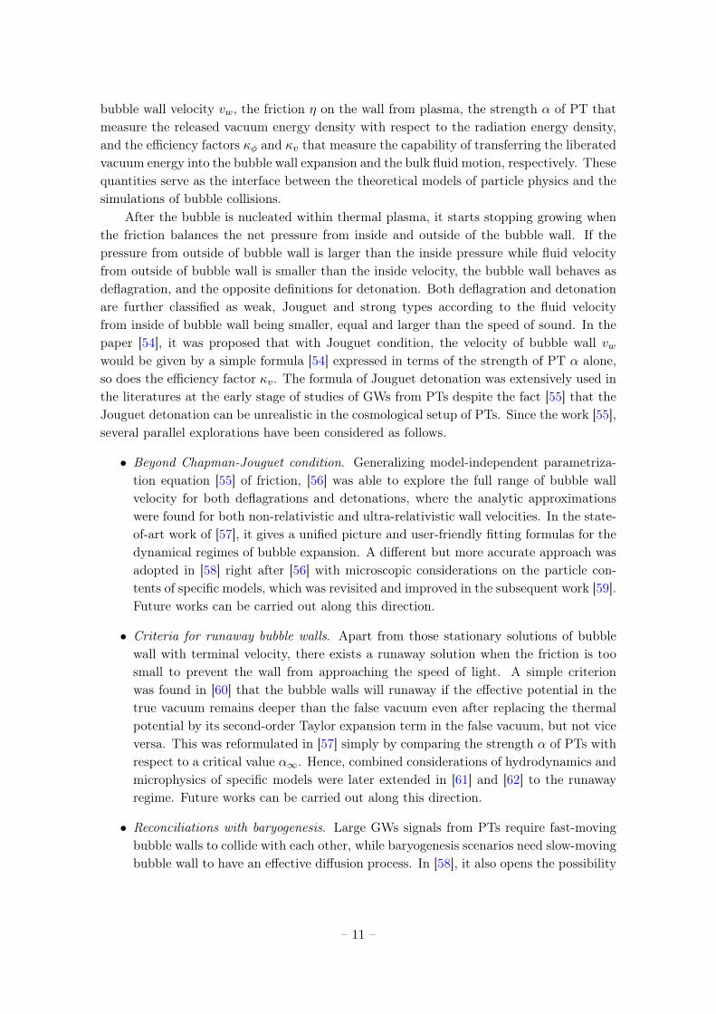
• Bubble collisions. It was first realized by Witten in [64] that the QCD PTs mightleave us with detectable GWs from violent bubble collisions with their peak frequencycharacterized by the size of bubbles when they collided and with their peak amplitudeestimated by the relative size of bubbles with respect to Hubble horizon at collision.Later on, this insight was generalized by Hogan in [65] to the case of EW PTs. In aseries of papers [66–69], the preliminary simulations were first implemented for bubblecollisions to capture the general features of GWs from PTs. It is found in [66, 67]that remarkably the spectrum of GWs from simulating the collision of two vacuumbubbles in Minkowski space only depends upon the grossest features of the bubblecollisions, namely, the strength α and duration β of PTs, which is similar to the resultof simulation for hundreds of vacuum bubbles [68]. As we have shown in Fig. 4, theenvelope approximation was proposed in [66–68] that the GWs are mainly generatedfrom the uncollided envelopes of colliding bubble walls and any GWs from the overlapregion can be neglected. The extension to the thermal bubble collisions was carriedout later in the simulation [69], where the Jouguet detonation mode was explicitlyused and the turbulent motion in fluid stirred by bubble collisions was appreciatedin this case. The state-of-the-art results of the GWs spectrum from PTs due tocolliding bubble walls were settled down in [70], which although disagreed with earlierstudy [71], they finally achieved consensus in [72]. Recently, under the thin-wall andenvelope approximations in flat background, it was claimed in [73] that the GWsspectrum can be estimated analytically without need of simulations. Future workscan be carried out along this direction from both theoretical and numerical points ofview.

– 12 –

R

true vacuumfalse vacuum

thin

shell

envelope

Figure 4. The schematic illustration of envelope approximation that the GWs are mainly generatedfrom the uncollided envelopes of colliding bubble walls and any GWs from the overlap region canbe neglected.

• Turbulent MHD. The possibility of generating GWs from turbulent motion of bulkfluid was mentioned long time ago in [64] as remnant of bubble collisions, whichwas first estimated in [69] as Kolmogorov spectrum under quadrupole approximation.Apart from above turbulent velocity field, the fully ionized plasma could also gener-ate the turbulent magnetic field under turbulent motion, which itself is also a sourceof GWs. The early analysis [74, 75] involving MHD exhibits three problems [37]:large-scale problem (addressed in [76, 77]), time-evolution problem (persisted in [77]and addressed in [76]) and dispersion-relation problem (corrected in [76, 77]). Thestate-of-art result of the GWs spectrum from PTs due to non-helical MHD turbu-lence was analytically established in [78], where it ignored the circularly polarizedGWs [79–85] from helical turbulence due to the macroscopic parity violation. Thenumerical simulations of relativistic MHD turbulence are certainly needed to makefurther confirmations for the above analytic results in the future.

• Sound waves. The possibility of generating GWs from sound waves was originallypointed out in [65], although, it left forgotten for a long time until recent revelationin [86], where envelope approximation for modeling the colliding bubble walls is aban-doned and the GWs should be dominated by the overlapping sound waves in the bulkfluid. The breakthrough findings of [86] were further quantitatively understood in

– 13 –

the updated simulations [87, 88] and theoretically modeled in [89], before which thepossibility of having an inverse acoustic cascade was investigated in [90], suggestingthe potentially very strong enhancement of the sound wave density at small wavenumber. Future works can be carried out along this direction for larger simulationswith more bubbles.

3.4 Gravitational Waves

The GWs from the strong first-order PTs are guaranteed through above three processes:bubble nucleation, bubble expansion and bubble percolation. The bubble nucleation re-quires a potential barrier in order to tunnel from the false vacuum to the true vacuum.The bubble expansion requires fast enough moving bubble walls in order to have strongsignals. The bubble percolation requires efficient collisions in order to dissipate releasedvacuum energy into bulk fluid motions. The fitting formulas of GWs spectrums from nu-merical simulations are well summarized in [36] and can be straightforwardly applied tothe particle physics models, where the strength α and duration β evaluated at nucleationtemperature T∗ along with the bubble wall velocity vw are obtained from the microscopicparticle physics models, whereas the efficiency factors κφ and κv are approximated from thefitting formulas in [57]. There leaves one last discussion of which particle physics modelscan exhibit first-order PT so that GWs can be generated.

The SM with phenomenological Higgs mechanism crosses over from the high-temperaturephase to low-temperature phase [91] if the Higgs boson mass is larger than the W bosonmass. To have GWs from first-order PTs, one has to go beyond SM (BSM) 3. Here, we givean incomplete list of these models with explicit discussions on GWs, which will be revisitedin the near future if we want to construct the reliable templates in order to extract the GWsignals from the stochastic background.

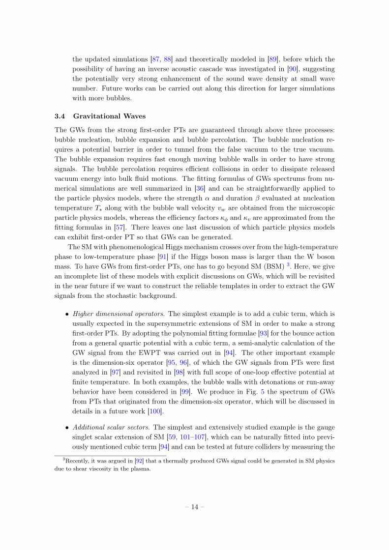
• Higher dimensional operators. The simplest example is to add a cubic term, which isusually expected in the supersymmetric extensions of SM in order to make a strongfirst-order PTs. By adopting the polynomial fitting formulae [93] for the bounce actionfrom a general quartic potential with a cubic term, a semi-analytic calculation of theGW signal from the EWPT was carried out in [94]. The other important exampleis the dimension-six operator [95, 96], of which the GW signals from PTs were firstanalyzed in [97] and revisited in [98] with full scope of one-loop effective potential atfinite temperature. In both examples, the bubble walls with detonations or run-awaybehavior have been considered in [99]. We produce in Fig. 5 the spectrum of GWsfrom PTs that originated from the dimension-six operator, which will be discussed indetails in a future work [100].

• Additional scalar sectors. The simplest and extensively studied example is the gaugesinglet scalar extension of SM [59, 101–107], which can be naturally fitted into previ-ously mentioned cubic term [94] and can be tested at future colliders by measuring the

3Recently, it was argued in [92] that a thermally produced GWs signal could be generated in SM physicsdue to shear viscosity in the plasma.

– 14 –

h2Ωbubble collision

h2Ωacoustic wave

h2ΩMHD turblence

h2Ωtot

eLISA-C1

eLISA-C2

eLISA-C3

10-5 10-4 10-3 10-2 0.1 1 10

10-17

10-13

10-9

10-5

f [Hz]

h2ΩGW(f)

Figure 5. The spectrum of GWs from PTs that originated from dimension-six operator with respectto the sensitivity curves of various configurations of eLISA project [37].

triple Higgs coupling precisely 4. The other important example is the charged scalarunder SM gauge group, of which the simplest realization is the two-Higgs-doubletmodel (2HDM). The GW from 2HDM was preliminarily analyzed in [109] and furtherstudied in [36] for the case of CP-conservation and recently revisited in [110] for thecase of CP-violation.

• Supersymmetric extensions. The capability of detecting GWs from PTs in Minimal Su-persymmetric Standard Model (MSSM) and Next-to-Minimal Supersymmetric Stan-dard Model (NMSSM) were first estimated in [111] and further explored in [112]. Boththe PTs from MSSM [59] and NMSSM [97] were thought to be not strong enough toproduce significant GW signals; however, the parameter space with strong first-orderPTs has been identified for a modified version of MSSM [113] and a general versionof NMSSM [62].

• Hidden dark sectors. The cosmological implications concerning with possible produc-tion of GWs from hidden dark sector were first explored in [114], and later discussedfor light GeV scalar [115], vector thermal dark matter [116], UV-conformal dark sec-tor [117], SU(N) dark sectors with nf flavors [118], dark U(1) gauge complex scalarsinglet [119], hidden sector with run-away bubble walls [120], and PTs involving suc-cessive hidden gauge symmetry breaking [121], dark matter asymmetry [122] and

4It has been exemplified in [108] with dimension-six operator that the future space-based interferometerscould probe the parameter spaces that are unreachable for the current particle colliders, but can have overlapwith the future particle colliders, therefore a cross-check is possible.

– 15 –

two-step transition [123]. The GWs from first-order PTs could be a unique probe forthese dark hidden sectors.

• Other BSM extensions. The GWs from first order PTs were also analyzed in the caseof extra dimensions [124–127], Peccei-Quinn PT [128], non-linear EWPT [129] andQCD PT [130–133].

4 The Gravitational Waves From Binary Systems

GW sources can be divided into two categories, one is deterministic and the other is stochas-tic. For example, the primordial GW produced by the quantum fluctuations and by PTsduring the early Universe belongs to the stochastic one. Due to the intrinsic random charac-ter, we cannot predict the waveform produced by the stochastic sources. The deterministicsources include two types. One type is predictable, while the other one is not. For example,the supernova is believed producing GWs. But the dynamics of supernova is too compli-cated to predict the related GW form. Another example is the foreground noise of LISAproduced by white dwarf-white dwarf binaries in our milky way galaxy [134–136]. Due tothe large number of such binaries, the combination of these GW signals makes the waveformunpredictable. In this section, we focus on the predictable GW sources. For such sources,we can construct theoretical model for gravitational waveform before GW detection exper-iment [137]. Then when the experiment data are ready, we can use matched filtering dataanalysis techniques to improve the GW detection sensitivity. And more, the theoreticalmodel can be used to realize the astronomy detection of the GW sources through matchedfiltering [138, 139].

Binary systems are among the most important and major sources for GW detectionprojects including PTA, space-based laser interferometer detectors such as eLISA, Taijiand Tianqin projects, ground-based laser interferometer detectors such as Advanced LIGO,Advanced Virgo, Kagra and others. The GW frequency of binary system around mergerstate can be characterized by the ISCO (most Inner Stable Circular Orbit) frequency:

fisco =1

63/22πM, (4.1)

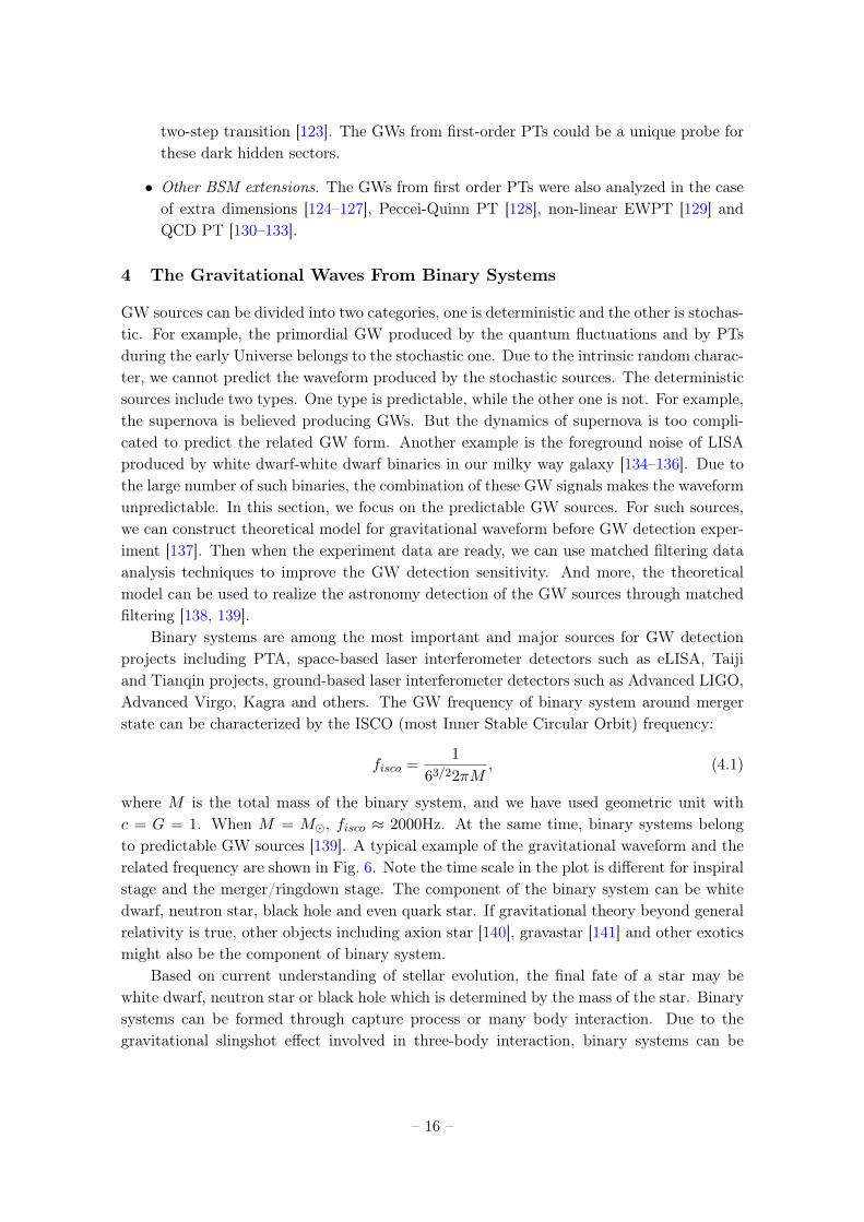
where M is the total mass of the binary system, and we have used geometric unit withc = G = 1. When M = M, fisco ≈ 2000Hz. At the same time, binary systems belongto predictable GW sources [139]. A typical example of the gravitational waveform and therelated frequency are shown in Fig. 6. Note the time scale in the plot is different for inspiralstage and the merger/ringdown stage. The component of the binary system can be whitedwarf, neutron star, black hole and even quark star. If gravitational theory beyond generalrelativity is true, other objects including axion star [140], gravastar [141] and other exoticsmight also be the component of binary system.

Based on current understanding of stellar evolution, the final fate of a star may bewhite dwarf, neutron star or black hole which is determined by the mass of the star. Binarysystems can be formed through capture process or many body interaction. Due to thegravitational slingshot effect involved in three-body interaction, binary systems can be

– 16 –

-0.4-0.3-0.2-0.1

0 0.1 0.2 0.3 0.4

h + R

/M

inspiral merger and ringdown

-0.4-0.3-0.2-0.1

00.10.20.3 0.4

h x R

/M

00.10.20.30.4 0.5

2000 4000 6000 8000

2πM

f

t/M 9000 9080 9160

Figure 6. Typical example of the gravitational waveform and the corresponding frequency. In thisexample, the binary system is a binary black hole with equal mass. And the two black holes arespinless. The whole evolution process of a binary black hole system includes inspiral, merger andringdown. But the boundary to distinguish these three stages is fuzzy. Compared to the inspiralstage, the merger and ringdown stages are much shorter. In this plot, we use different time scalefor inspiral and merger/ringdown stage in order to make the merger/ringdown stage clearer.

formed through many body interaction. Because a binary system is dynamically stable,binary systems are expected to be quite common in our Universe.

The direct detection of GWs opens the GW astronomy. Through this new window toour Universe, GWs will not only bring us many new observations on kinds of objects in theUniverse, but also give us many insights on fundamental physical theory. For example, blackhole is a mystery from quantum gravity theory view. Especially, black hole presents us aninformation loss puzzle. Is it possible the black hole horizon be replaced with other objectssuch as firewall or anything else? Or any experiments present evidence that black holehorizon really exists? Unfortunately, one cannot get observational proof of the existenceof a black hole event horizon based on EM waves [142]. In contrast, it is possible to useGW observation to give a direct proof of the existence of a black hole event horizon [143].Currently, these promising aims can be most possibly achieved by predictable GW sources,especially binary systems. In order to realize these aims, we have to construct accurateenough gravitational waveform model for binary systems. There are three kinds of methodsavailable to treat binary systems. They are PN approximation, numerical relativity andblack hole perturbation method which are widely used for early inspiral stage, plunge andmerger stage, and post merger stage, respectively.

– 17 –

4.1 Post-Newtonian Approximation

Based on quadrupole formula [144], we can estimate the GWs related to a binary system:

h+ = −Mr

2Ω2R2(1 + cos2 θ) cos[2Ω(t− r)], (4.2)

h× = −Mr

4Ω2R2 cos θ sin[2Ω(t− r)], (4.3)

where (r, θ, φ) is the position of the observer with respect to the binary, M , R and Ω arethe total mass, the separation and the mutual orbiting frequency of the two componentsof the binary. Here h+ and h× correspond to two polarization modes of GWs. These twomodes are related to the dynamical metric form as

ds2 = −dt2 + dr2 + r2(1 + h+)dθ2 + r2 sin2 θ(1− h+)dφ2 + 2r2 sin θh×dθdφ, (4.4)

with (t, r, θ, φ) corresponding to the transverse-traceless gauge [145]. Here we need pointout two points. First one is that the planer wave approximation has been taken in theabove equation which is reasonable because the field point is very far away from the source.The second is that above estimation about h+ and h× is only leading order of the PNapproximation which is reasonable because the weak GW source moves slowly. For mostrealistic GW sources, these approximations will break down. Even for cases in which theapproximation is reasonable, above approximation cannot satisfy the need of GW detec-tion [146, 147]. For example, when the two components of a binary system are some faraway, they move slowly. So, this kind of situation corresponds to weak and moving slowlyGW source. Although the above approximation is reasonable, the accuracy is not goodenough. Then, more PN order corrections are needed to improve the accuracy [148].

The theoretical framework of the PN approximation for the processing of binary systemsconsists of two parts: the dynamics of binary components and the GWform. In order toconstruct the GW model, we need to solve the binary dynamics, and then put the solutioninto the waveform theory part to get the explicit GW model. In general, the dynamicalequations of the PN approximation are a highly nonlinear system of ordinary differentialequations. In that case, the numerical method has to be employed to get the solution.GW models in which the GWform is expressed in time domain include TaylorT2, TaylorT4and others [149]. Through stationary phase approximation, the post-Newtonian equationscan be transformed into a frequency domain problem, and fortunately an approximateanalytical expression can be obtained. Such a model is typically represented by the TaylorF2model. Corrected by the binary black hole spin dynamics, especially the effect of the orbitalprecession, the TaylorF2 model is modified and improved by single and double precessionmodel [150, 151]. The TaylorT2 model is replaced by the X model when the elliptic orbitof the binary system is considered [152]. The theoretical model of the TaylorF2 model isextended to the elliptic orbit binary system including the post-circular model [153] and theenhanced post-circular model [154, 155].

4.2 Numerical Relativity

Applying numerical methods to solve the Einstein equation is the topic of numerical rela-tivity. Currently, the numerical relativity can only deal with the problem of GW modeling

– 18 –

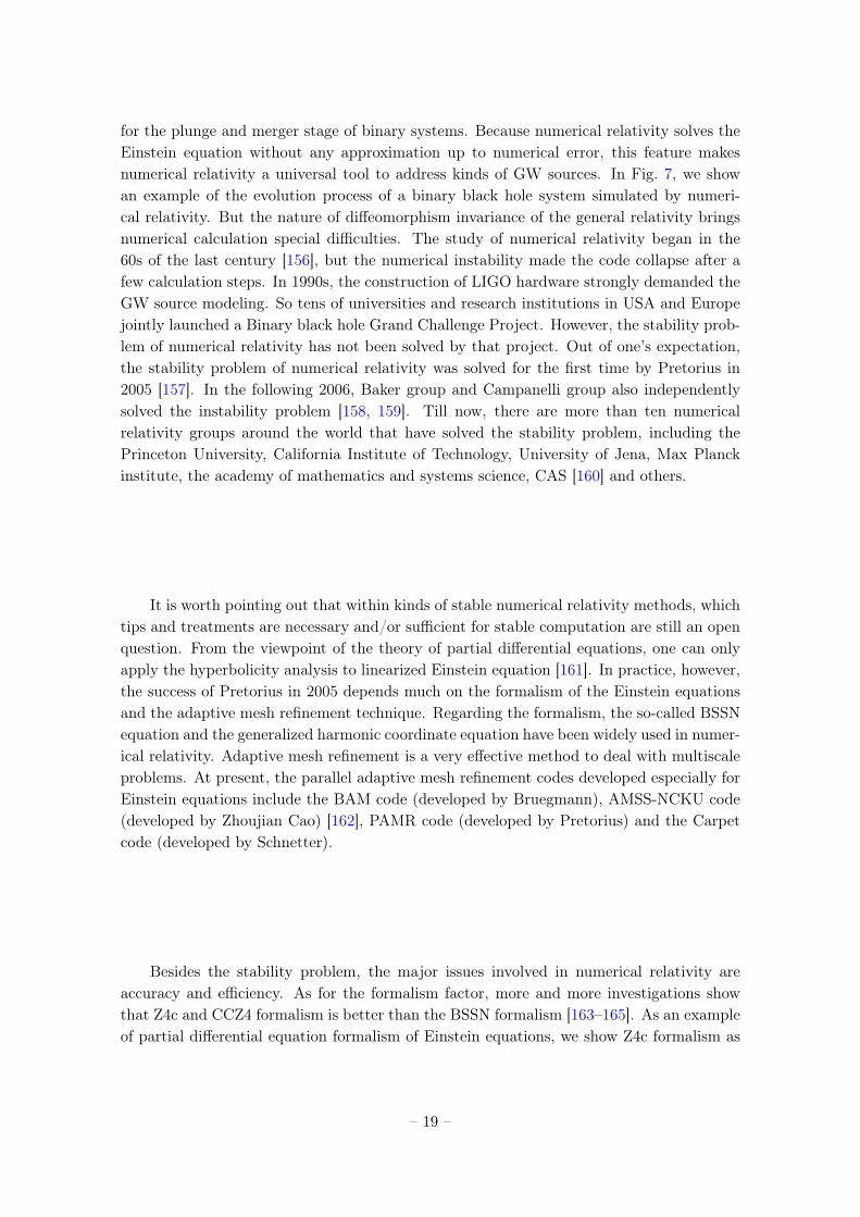
for the plunge and merger stage of binary systems. Because numerical relativity solves theEinstein equation without any approximation up to numerical error, this feature makesnumerical relativity a universal tool to address kinds of GW sources. In Fig. 7, we showan example of the evolution process of a binary black hole system simulated by numeri-cal relativity. But the nature of diffeomorphism invariance of the general relativity bringsnumerical calculation special difficulties. The study of numerical relativity began in the60s of the last century [156], but the numerical instability made the code collapse after afew calculation steps. In 1990s, the construction of LIGO hardware strongly demanded theGW source modeling. So tens of universities and research institutions in USA and Europejointly launched a Binary black hole Grand Challenge Project. However, the stability prob-lem of numerical relativity has not been solved by that project. Out of one’s expectation,the stability problem of numerical relativity was solved for the first time by Pretorius in2005 [157]. In the following 2006, Baker group and Campanelli group also independentlysolved the instability problem [158, 159]. Till now, there are more than ten numericalrelativity groups around the world that have solved the stability problem, including thePrinceton University, California Institute of Technology, University of Jena, Max Planckinstitute, the academy of mathematics and systems science, CAS [160] and others.

It is worth pointing out that within kinds of stable numerical relativity methods, whichtips and treatments are necessary and/or sufficient for stable computation are still an openquestion. From the viewpoint of the theory of partial differential equations, one can onlyapply the hyperbolicity analysis to linearized Einstein equation [161]. In practice, however,the success of Pretorius in 2005 depends much on the formalism of the Einstein equationsand the adaptive mesh refinement technique. Regarding the formalism, the so-called BSSNequation and the generalized harmonic coordinate equation have been widely used in numer-ical relativity. Adaptive mesh refinement is a very effective method to deal with multiscaleproblems. At present, the parallel adaptive mesh refinement codes developed especially forEinstein equations include the BAM code (developed by Bruegmann), AMSS-NCKU code(developed by Zhoujian Cao) [162], PAMR code (developed by Pretorius) and the Carpetcode (developed by Schnetter).

Besides the stability problem, the major issues involved in numerical relativity areaccuracy and efficiency. As for the formalism factor, more and more investigations showthat Z4c and CCZ4 formalism is better than the BSSN formalism [163–165]. As an exampleof partial differential equation formalism of Einstein equations, we show Z4c formalism as

– 19 –

Figure 7. Typical evolution of binary black hole simulated by numerical relativity. The yellowregion corresponds to the highly curved region which is roughly the position of black holes. Thefour snapshots correspond to inspiral, merger and ringdown stages. This result is simulated byAMSS-NCKU software.

following, which is proposed first time in 3D form in [164]:

∂tχ =2

3χ[α(K + 2Θ)−Diβ

i], (4.5)

∂tγij = −2αAij + 2γk(i∂j)βk − 2

3γij∂kβ

k + βk∂kγij , (4.6)

∂tK = −DiDiα+ α[AijA

ij +1

3(K + 2Θ)2

+ κ1(1− κ2)Θ] + 4πα[S + ρADM] + βi∂iK, (4.7)

∂tAij = χ[−DiDjα+ α(Rij − 8πSij)]tf + α[(K + 2Θ)Aij

− 2AikAkj ] + 2Ak(i∂j)β

k − 2

3Aij∂kβ

k + βk∂kAij , (4.8)

∂tΘ =1

2α[R− AijAij +

2

3(K + 2Θ)2 − 16πρADM

− 2κ1(2 + κ2)Θ]

+ βi∂iΘ, (4.9)

∂tΓi = γjk∂j∂kβ

i +1

3γij∂j∂kβ

k − 2Aij∂jα

+ 2α[ΓijkA

jk − 3

2Aij∂j lnχ− 1

3γij∂j(2K + Θ)

− κ1(Γi − Γdi)− 8πγijSj

]+

2

3Γd

i∂jβj − Γd

j∂jβi

+ βj∂jΓi. (4.10)

– 20 –

The unknown functions which need to be solved numerically are listed in the left-hand sideof the above equations. For the meaning of the notations used in the above equations,we refer our readers to [164]. Spectral method, finite difference method and finite elementmethod are three categories of numerical methods for partial differential equations. The vastmajority of numerical relativity groups take the finite differential method. The SpEC code ofCalifornia Institute of Technology uses spectral method. On the other hand, the applicationof finite element method into numerical relativity is still very few [166]. The spectralmethod has good computational efficiency due to its exponential convergence. However, thecharacteristics of its global data exchange limits its ability of parallel computing. The finitedifference method working with domain decomposition algorithm can achieve good parallelcomputing efficiency. In order to deal with the multiscale characteristics of astrophysics,the refinement of the multilayer data structure is essential in the finite difference method.However, this method limits the number of cores for parallel computation by a single datalayer, thus limits the strong parallel scalability. In contrast, the finite element methodcan combine the exponential convergence of the spectral method and the high parallelscalability of the difference method. Therefore, in principle, it is expected that the finiteelement calculation of the Einstein equations can achieve good strong parallel scalability.However, it is still an issue to construct the weak form of the Einstein equations, and torealize large-scale scientific computation [137, 139].

Now the major challenges to numerical relativity placed by GW source modeling arethe calculation of binary systems with mass ratio more than 100 to 1 and the well-convergedsimulation of binary systems including neutron stars [138].

4.3 Black Hole Perturbation

After the merger of the binary components, the system will ringdown and finally settledown to a Kerr black hole. If the two components are white dwarf and/or neutron star,the final remnant could be a stable neutron star. Here, we only concern with the casewith Kerr black hole as the final product. Then the ringdown stage can be describedby perturbation of a Kerr black hole. The black hole perturbation theory was pioneeredby Regge, Wheeler and Zerilli [167, 168] in which perturbation around a Schwarzschildblack hole was considered. Teukolsky investigated the perturbation of a Kerr black holeon spacetime curvature level [169, 170]. The former is called the Regge-Wheeler-Zerilliequation, and the latter is called the Teukolsky equation. The perturbation method usedby Teukolsky is also valid to Schwarzschild black hole. For Schwarzschild black hole, Regge-Wheeler-Zerilli method and Teukolsky method is equivalent [171]. In the early 70s of thelast century, some scholars have begun to use the Regge-Wheeler-Zerilli equation to studythe associated GW for a test particle falling into a black hole [172–174]. Because theTeukolsky equation admits spin of a black hole, it is valid more extensively than the Regge-Wheeler-Zerilli equation. In recent years, there have been many works using the Teukolskyequation to calculate the GWs.

The Teukolsky equation can be solved by the PN approximation method (note thatthe Teukolsky equation is the target in question here, instead of Einstein equation itselflike what described in the above subsection) or through numerical method. The PN ap-

– 21 –

proximation method was mainly developed by Mano, Suzuki, Takasugi and others. Theseauthors developed some hypergeometric functions and Coulomb wave functions to approx-imate the homogeneous solution of the Teukolsky equation [175, 176]. Later on, Fujita andhis coworkers applied PN approximation method to these analytical solutions to calculatethe GWform and the related energy flux for extreme mass ratio binary systems. Currently,22PN accuracy for Schwarzschild black hole and 11PN accuracy for Kerr black hole havebeen achieved [177, 178]. However, such accuracy still do not yet satisfy the requirementof GW detection experiment [179].

The numerical methods to solve the Teukolsky equation can be divided into two cate-gories: frequency domain method and time domain method. The frequency domain methoddivides the original Teukolsky equation into two ordinary differential equations through vari-able separating method and the Fourier expansion [169]. Regarding the radial equation,we can transform it to Sasaki-Nakamura equation before solving it numerically [180]. TheTeukolsky equation can only provide the energy flux and the GWs. In order to providethe orbit of the test particle, Hughes and his coworkers applied adiabatic approximationmethod to the geodesic equation to treat the inspiral [181]. Now this kind of approxima-tion has become an important method to treat binary systems with extreme mass ratio.Different from the usual finite difference numerical method, Fujita and Tagoshi used thehypergeometric function and the Coulomb wave function to expand the original equationswhich gives a quicker and more accurate numerical method [182]. The numerical methodin time domain needs to solve a set of 2+1 partial differential equations. At present, onemainly uses the finite difference method to solve the problem (but see [183] for the finiteelement method). Due to the extreme mass ratio of the involved binary system, the relatedGW signal may last several years. Although the computation required by Teukolsky equa-tion is much simpler than numerical relativity, how to improve the computational efficiencyof the Teukolsky equation is also a great challenge for GW source modeling.

4.4 Cosmological Probes

In 1986, Schutz showed that from the GWs one can infer the Hubble constant by using thefact that the GWs from the binary systems encode the absolute distance information [184].The inspiraling and merging compact binaries consisting of neutron stars and black holescan be considered as standard candles, or “standard sirens”. The name of “siren” is dueto the fact that the GW detectors are omni-directional and detect coherently the phaseof the wave, which makes them in many ways more like microphones for sound than likeconventional telescopes. For an expanding Universe, the chirp waveform of the GW can begeneralized to the cosmological case by multiplying all masses by the factor 1 + z and thephysical distance D can be replaced by the luminosity distance dL [185, 186]. In fact, thewaveform h produced by compact binary inspirals during the inspiral phase is theoreticallywell described by the analytical solution:

h× =4

dL(z)

(GMc(z)

c2

)5/3(πfc

)2/3

cos ι sin[Φ(f)] , (4.11)

– 22 –

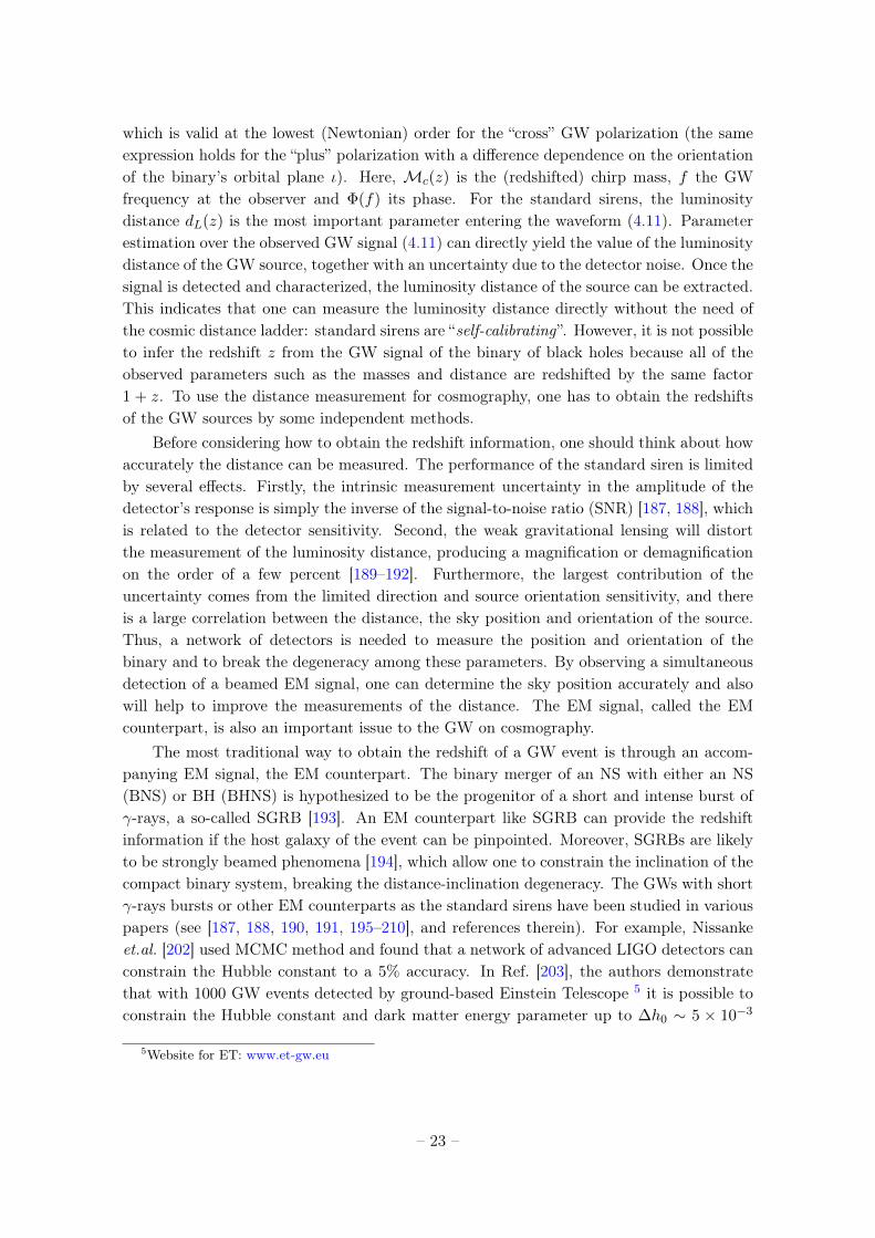
which is valid at the lowest (Newtonian) order for the “cross” GW polarization (the sameexpression holds for the “plus” polarization with a difference dependence on the orientationof the binary’s orbital plane ι). Here, Mc(z) is the (redshifted) chirp mass, f the GWfrequency at the observer and Φ(f) its phase. For the standard sirens, the luminositydistance dL(z) is the most important parameter entering the waveform (4.11). Parameterestimation over the observed GW signal (4.11) can directly yield the value of the luminositydistance of the GW source, together with an uncertainty due to the detector noise. Once thesignal is detected and characterized, the luminosity distance of the source can be extracted.This indicates that one can measure the luminosity distance directly without the need ofthe cosmic distance ladder: standard sirens are “self-calibrating”. However, it is not possibleto infer the redshift z from the GW signal of the binary of black holes because all of theobserved parameters such as the masses and distance are redshifted by the same factor1 + z. To use the distance measurement for cosmography, one has to obtain the redshiftsof the GW sources by some independent methods.

Before considering how to obtain the redshift information, one should think about howaccurately the distance can be measured. The performance of the standard siren is limitedby several effects. Firstly, the intrinsic measurement uncertainty in the amplitude of thedetector’s response is simply the inverse of the signal-to-noise ratio (SNR) [187, 188], whichis related to the detector sensitivity. Second, the weak gravitational lensing will distortthe measurement of the luminosity distance, producing a magnification or demagnificationon the order of a few percent [189–192]. Furthermore, the largest contribution of theuncertainty comes from the limited direction and source orientation sensitivity, and thereis a large correlation between the distance, the sky position and orientation of the source.Thus, a network of detectors is needed to measure the position and orientation of thebinary and to break the degeneracy among these parameters. By observing a simultaneousdetection of a beamed EM signal, one can determine the sky position accurately and alsowill help to improve the measurements of the distance. The EM signal, called the EMcounterpart, is also an important issue to the GW on cosmography.

The most traditional way to obtain the redshift of a GW event is through an accom-panying EM signal, the EM counterpart. The binary merger of an NS with either an NS(BNS) or BH (BHNS) is hypothesized to be the progenitor of a short and intense burst ofγ-rays, a so-called SGRB [193]. An EM counterpart like SGRB can provide the redshiftinformation if the host galaxy of the event can be pinpointed. Moreover, SGRBs are likelyto be strongly beamed phenomena [194], which allow one to constrain the inclination of thecompact binary system, breaking the distance-inclination degeneracy. The GWs with shortγ-rays bursts or other EM counterparts as the standard sirens have been studied in variouspapers (see [187, 188, 190, 191, 195–210], and references therein). For example, Nissankeet.al. [202] used MCMC method and found that a network of advanced LIGO detectors canconstrain the Hubble constant to a 5% accuracy. In Ref. [203], the authors demonstratethat with 1000 GW events detected by ground-based Einstein Telescope 5 it is possible toconstrain the Hubble constant and dark matter energy parameter up to ∆h0 ∼ 5 × 10−3

5Website for ET: www.et-gw.eu

– 23 –

and ∆Ωm ∼ 0.02 using Fisher matrix approach, which was also found by Cai et al. [188]using MCMC method. Furthermore, Cai et al. used the Gaussian Process method andfound that the equation of state of the dark energy can be constrained to ∆w(z) ∼ 0.03 inthe low redshift region, which gives a better constraint than Ref. [203]. For the space-baseddetector LISA 6, the expansion of the Universe and interacting dark energy have also beenstudied by Refs. [208, 210].

There also exist other methods to infer the redshift information of the GW events, suchas galaxy catalog proposed by Schutz [184], neutron star mass distribution [195, 211], andthe tidal deformation of neutron stars [212, 213]. Measuring the redshift associated witha GW event is one of the biggest challenges in the future, see [214]; however, for a newGW standard sirens probe without redshift information by utilizing those BH binaries tobe a tracer of the large-scale structure [215]. In addition, the spin of BH can also helpus estimate the GW’s parameters. GWs as the standard sirens to probe the cosmologicalparameters can provide an independent and complementary alternative to current experi-ments. It is expected that combining GW data with other astronomical observations suchas supernovae, and adopting a better data analysis approach, the cosmological parameterscould be constrained more precisely than the current situation.

5 Conclusions

The direct detection of GWs by LIGO initiates a new era of GW astronomy and GWcosmology. The GW physics is not only related to gravitational physics, but also closelyrelated to particle physics, cosmology and astrophysics. The GWs provide us a new powerfultool to reveal various secrets of the nature. Indeed, a lot of relevant papers have appearedsince the announcement of the direct detection of GWs. In this paper, we have brieflyintroduced three kinds of GW sources and relevant physics. They are GWs producedduring inflation and preheating in the early Universe, from cosmic PTs and dynamics ofcompact binary systems, respectively. We also have discussed in a simple way the GWs asstandard siren in the evolution of the Universe. Due to the limitation of space, we are notable to discuss all aspects of GW physics, but only focus on some main issues. Of course,it is also impossible to list a complete list of the references, quite probably some importantreferences are missed here, we should apologize for this.

Acknowledgments

This work is supported in part by the National Natural Science Foundation of China GrantsNo.11690021, No.11690022, No.11690023, No.11622546, No.11575272, No.11375260 andNo.11335012, in part by the Strategic Priority Research Program of CAS Grant No.XDB23030100and by the Key Research Program of Frontier Sciences of CAS Grant No.QYZDJ-SSWSYS006.

6Website for eLISA: www.elisascience.org

– 24 –

References

[1] Virgo, LIGO Scientific collaboration, B. P. Abbott et al., Observation of GravitationalWaves from a Binary Black Hole Merger, Phys. Rev. Lett. 116 (2016) 061102, [1602.03837].

[2] Virgo, LIGO Scientific collaboration, B. P. Abbott et al., GW151226: Observation ofGravitational Waves from a 22-Solar-Mass Binary Black Hole Coalescence, Phys. Rev. Lett.116 (2016) 241103, [1606.04855].

[3] A. Einstein, Approximative Integration of the Field Equations of Gravitation, Sitzungsber.Preuss. Akad. Wiss. Berlin (Math. Phys.) 1916 (1916) 688–696.

[4] A. Einstein, Über Gravitationswellen, Sitzungsber. Preuss. Akad. Wiss. Berlin (Math.Phys.) 1918 (1918) 154–167.

[5] P. R. Saulson, Josh Goldberg and the physical reality of gravitational waves, Gen. Rel. Grav.43 (2011) 3289–3299.

[6] H. Bondi, Plane gravitational waves in general relativity, Nature 179 (1957) 1072–1073.

[7] H. Bondi, F. A. E. Pirani and I. Robinson, Gravitational waves in general relativity. 3.Exact plane waves, Proc. Roy. Soc. Lond. A251 (1959) 519–533.

[8] A. H. Guth, The Inflationary Universe: A Possible Solution to the Horizon and FlatnessProblems, Phys. Rev. D23 (1981) 347–356.

[9] A. Albrecht and P. J. Steinhardt, Cosmology for Grand Unified Theories with RadiativelyInduced Symmetry Breaking, Phys. Rev. Lett. 48 (1982) 1220–1223.

[10] A. D. Linde, A New Inflationary Universe Scenario: A Possible Solution of the Horizon,Flatness, Homogeneity, Isotropy and Primordial Monopole Problems, Phys. Lett. B108(1982) 389–393.

[11] Planck collaboration, P. A. R. Ade et al., Planck 2015 results. XX. Constraints oninflation, Astron. Astrophys. 594 (2016) A20, [1502.02114].

[12] A. A. Starobinsky, A New Type of Isotropic Cosmological Models Without Singularity, Phys.Lett. B91 (1980) 99–102.

[13] Z.-K. Guo, D. J. Schwarz and Y.-Z. Zhang, Reconstruction of the primordial powerspectrum from CMB data, JCAP 1108 (2011) 031, [1105.5916].

[14] Z.-K. Guo and Y.-Z. Zhang, Uncorrelated estimates of the primordial power spectrum,JCAP 1111 (2011) 032, [1109.0067].

[15] B. Hu, J.-W. Hu, Z.-K. Guo and R.-G. Cai, Reconstruction of the primordial power spectrawith Planck and BICEP2 data, Phys. Rev. D90 (2014) 023544, [1404.3690].

[16] C. Armendariz-Picon, T. Damour and V. F. Mukhanov, k - inflation, Phys. Lett. B458(1999) 209–218, [hep-th/9904075].

[17] Z.-K. Guo and D. J. Schwarz, Power spectra from an inflaton coupled to the Gauss-Bonnetterm, Phys. Rev. D80 (2009) 063523, [0907.0427].

[18] Z.-K. Guo and D. J. Schwarz, Slow-roll inflation with a Gauss-Bonnet correction, Phys.Rev. D81 (2010) 123520, [1001.1897].

[19] P.-X. Jiang, J.-W. Hu and Z.-K. Guo, Inflation coupled to a Gauss-Bonnet term, Phys. Rev.D88 (2013) 123508, [1310.5579].

– 25 –

[20] T. Kobayashi, M. Yamaguchi and J. Yokoyama, Generalized G-inflation: Inflation with themost general second-order field equations, Prog. Theor. Phys. 126 (2011) 511–529,[1105.5723].

[21] S. Matarrese, S. Mollerach and M. Bruni, Second order perturbations of the Einstein-deSitter universe, Phys. Rev. D58 (1998) 043504, [astro-ph/9707278].

[22] N. Bartolo, S. Matarrese, A. Riotto and A. Vaihkonen, The Maximal Amount ofGravitational Waves in the Curvaton Scenario, Phys. Rev. D76 (2007) 061302, [0705.4240].

[23] M. Biagetti, M. Fasiello and A. Riotto, Enhancing Inflationary Tensor Modes throughSpectator Fields, Phys. Rev. D88 (2013) 103518, [1305.7241].

[24] M. Biagetti, E. Dimastrogiovanni, M. Fasiello and M. Peloso, Gravitational Waves andScalar Perturbations from Spectator Fields, JCAP 1504 (2015) 011, [1411.3029].

[25] J. L. Cook and L. Sorbo, Particle production during inflation and gravitational wavesdetectable by ground-based interferometers, Phys. Rev. D85 (2012) 023534, [1109.0022].

[26] A. Albrecht, P. J. Steinhardt, M. S. Turner and F. Wilczek, Reheating an InflationaryUniverse, Phys. Rev. Lett. 48 (1982) 1437.

[27] J. H. Traschen and R. H. Brandenberger, Particle Production During Out-of-equilibriumPhase Transitions, Phys. Rev. D42 (1990) 2491–2504.

[28] S. Y. Khlebnikov and I. I. Tkachev, Relic gravitational waves produced after preheating,Phys. Rev. D56 (1997) 653–660, [hep-ph/9701423].

[29] G. N. Felder and I. Tkachev, LATTICEEASY: A Program for lattice simulations of scalarfields in an expanding universe, Comput. Phys. Commun. 178 (2008) 929–932,[hep-ph/0011159].

[30] R. Easther and E. A. Lim, Stochastic gravitational wave production after inflation, JCAP0604 (2006) 010, [astro-ph/0601617].

[31] R. Easther, J. T. Giblin, Jr. and E. A. Lim, Gravitational Wave Production At The End OfInflation, Phys. Rev. Lett. 99 (2007) 221301, [astro-ph/0612294].

[32] C. Guzzetti, M., N. Bartolo, M. Liguori and S. Matarrese, Gravitational waves frominflation, Riv. Nuovo Cim. 39 (2016) 399–495, [1605.01615].

[33] BICEP2, Planck collaboration, P. A. R. Ade et al., Joint Analysis ofBICEP2/KeckArray and Planck Data, Phys. Rev. Lett. 114 (2015) 101301, [1502.00612].

[34] L. A. Boyle and P. J. Steinhardt, Probing the early universe with inflationary gravitationalwaves, Phys. Rev. D77 (2008) 063504, [astro-ph/0512014].

[35] N. Bartolo et al., Science with the space-based interferometer LISA. IV: Probing inflationwith gravitational waves, JCAP 1612 (2016) 026, [1610.06481].

[36] C. Caprini et al., Science with the space-based interferometer eLISA. II: Gravitationalwaves from cosmological phase transitions, JCAP 1604 (2016) 001, [1512.06239].

[37] P. Binetruy, A. Bohe, C. Caprini and J.-F. Dufaux, Cosmological Backgrounds ofGravitational Waves and eLISA/NGO: Phase Transitions, Cosmic Strings and OtherSources, JCAP 1206 (2012) 027, [1201.0983].

[38] S. R. Coleman, The Fate of the False Vacuum. 1. Semiclassical Theory, Phys. Rev. D15(1977) 2929–2936.

– 26 –

[39] C. G. Callan, Jr. and S. R. Coleman, The Fate of the False Vacuum. 2. First QuantumCorrections, Phys. Rev. D16 (1977) 1762–1768.

[40] S. R. Coleman and F. De Luccia, Gravitational Effects on and of Vacuum Decay, Phys.Rev. D21 (1980) 3305.

[41] A. D. Linde, Decay of the False Vacuum at Finite Temperature, Nucl. Phys. B216 (1983)421.

[42] A. D. Linde, Fate of the False Vacuum at Finite Temperature: Theory and Applications,Phys. Lett. B100 (1981) 37–40.

[43] D. Curtin, P. Meade and H. Ramani, Thermal Resummation and Phase Transitions,1612.00466.

[44] P. John, Bubble wall profiles with more than one scalar field: A Numerical approach, Phys.Lett. B452 (1999) 221–226, [hep-ph/9810499].

[45] T. Konstandin and S. J. Huber, Numerical approach to multi-dimensional phase transitions,Journal of Cosmology and Astroparticle Physics 2006 (2006) 021.

[46] C. L. Wainwright, CosmoTransitions: Computing Cosmological Phase TransitionTemperatures and Bubble Profiles with Multiple Fields, Comput. Phys. Commun. 183(2012) 2006–2013, [1109.4189].

[47] S. Akula, C. Balázs and G. A. White, Semi-analytic techniques for calculating bubble wallprofiles, Eur. Phys. J. C76 (2016) 681, [1608.00008].

[48] S. J. Parke, Gravity, the Decay of the False Vacuum and the New Inflationary UniverseScenario, Phys. Lett. B121 (1983) 313–315.

[49] C. Baccigalupi, L. Amendola, P. Fortini and F. Occhionero, The Stochastic gravitationalbackground from inflationary phase transitions, Phys. Rev. D56 (1997) 4610–4617,[gr-qc/9709044].

[50] D. Chialva, Gravitational waves from first order phase transitions during inflation, Phys.Rev. D83 (2011) 023512, [1004.2051].

[51] H. Jiang, T. Liu, S. Sun and Y. Wang, Echoes of Inflationary First-Order PhaseTransitions in the CMB, Phys. Lett. B765 (2017) 339–343, [1512.07538].

[52] G. Barenboim and W.-I. Park, Gravitational waves from first order phase transitions as aprobe of an early matter domination era and its inverse problem, Phys. Lett. B759 (2016)430–438, [1605.03781].

[53] M. Artymowski, M. Lewicki and J. D. Wells, Gravitational wave and collider implications ofelectroweak baryogenesis aided by non-standard cosmology, 1609.07143.

[54] P. J. Steinhardt, Relativistic Detonation Waves and Bubble Growth in False Vacuum Decay,Phys. Rev. D25 (1982) 2074.

[55] H. Kurki-Suonio and M. Laine, Supersonic deflagrations in cosmological phase transitions,Phys. Rev. D51 (1995) 5431–5437, [hep-ph/9501216].

[56] A. Megevand and A. D. Sanchez, Detonations and deflagrations in cosmological phasetransitions, Nucl. Phys. B820 (2009) 47–74, [0904.1753].

[57] J. R. Espinosa, T. Konstandin, J. M. No and G. Servant, Energy Budget of CosmologicalFirst-order Phase Transitions, JCAP 1006 (2010) 028, [1004.4187].

– 27 –

[58] A. Megevand and A. D. Sanchez, Velocity of electroweak bubble walls, Nucl. Phys. B825(2010) 151–176, [0908.3663].

[59] L. Leitao, A. Megevand and A. D. Sanchez, Gravitational waves from the electroweak phasetransition, JCAP 1210 (2012) 024, [1205.3070].

[60] D. Bodeker and G. D. Moore, Can electroweak bubble walls run away?, JCAP 0905 (2009)009, [0903.4099].

[61] L. Leitao and A. Megevand, Hydrodynamics of ultra-relativistic bubble walls, Nucl. Phys.B905 (2016) 45–72, [1510.07747].

[62] S. J. Huber, T. Konstandin, G. Nardini and I. Rues, Detectable Gravitational Waves fromVery Strong Phase Transitions in the General NMSSM, JCAP 1603 (2016) 036,[1512.06357].

[63] J. M. No, Large Gravitational Wave Background Signals in Electroweak BaryogenesisScenarios, Phys. Rev. D84 (2011) 124025, [1103.2159].

[64] E. Witten, Cosmic Separation of Phases, Phys. Rev. D30 (1984) 272–285.

[65] C. J. Hogan, Gravitational radiation from cosmological phase transitions, Mon. Not. Roy.Astron. Soc. 218 (1986) 629–636.

[66] A. Kosowsky, M. S. Turner and R. Watkins, Gravitational radiation from colliding vacuumbubbles, Phys. Rev. D45 (1992) 4514–4535.

[67] A. Kosowsky, M. S. Turner and R. Watkins, Gravitational waves from first ordercosmological phase transitions, Phys. Rev. Lett. 69 (1992) 2026–2029.

[68] A. Kosowsky and M. S. Turner, Gravitational radiation from colliding vacuum bubbles:envelope approximation to many bubble collisions, Phys. Rev. D47 (1993) 4372–4391,[astro-ph/9211004].

[69] M. Kamionkowski, A. Kosowsky and M. S. Turner, Gravitational radiation from first orderphase transitions, Phys. Rev. D49 (1994) 2837–2851, [astro-ph/9310044].

[70] S. J. Huber and T. Konstandin, Gravitational Wave Production by Collisions: MoreBubbles, JCAP 0809 (2008) 022, [0806.1828].

[71] C. Caprini, R. Durrer and G. Servant, Gravitational wave generation from bubble collisionsin first-order phase transitions: An analytic approach, Phys. Rev. D77 (2008) 124015,[0711.2593].

[72] C. Caprini, R. Durrer, T. Konstandin and G. Servant, General Properties of theGravitational Wave Spectrum from Phase Transitions, Phys. Rev. D79 (2009) 083519,[0901.1661].

[73] R. Jinno and M. Takimoto, Gravitational waves from bubble collisions: analytic derivation,Phys. Rev. D95 (2017) 024009, [1605.01403].

[74] A. Kosowsky, A. Mack and T. Kahniashvili, Gravitational radiation from cosmologicalturbulence, Phys. Rev. D66 (2002) 024030, [astro-ph/0111483].

[75] A. D. Dolgov, D. Grasso and A. Nicolis, Relic backgrounds of gravitational waves fromcosmic turbulence, Phys. Rev. D66 (2002) 103505, [astro-ph/0206461].

[76] C. Caprini and R. Durrer, Gravitational waves from stochastic relativistic sources:Primordial turbulence and magnetic fields, Phys. Rev. D74 (2006) 063521,[astro-ph/0603476].

– 28 –

[77] G. Gogoberidze, T. Kahniashvili and A. Kosowsky, The Spectrum of GravitationalRadiation from Primordial Turbulence, Phys. Rev. D76 (2007) 083002, [0705.1733].

[78] C. Caprini, R. Durrer and G. Servant, The stochastic gravitational wave background fromturbulence and magnetic fields generated by a first-order phase transition, JCAP 0912(2009) 024, [0909.0622].

[79] T. Kahniashvili, G. Gogoberidze and B. Ratra, Polarized cosmological gravitational wavesfrom primordial helical turbulence, Phys. Rev. Lett. 95 (2005) 151301, [astro-ph/0505628].

[80] T. Kahniashvili, G. Gogoberidze and B. Ratra, Gravitational Radiation from PrimordialHelical MHD Turbulence, Phys. Rev. Lett. 100 (2008) 231301, [0802.3524].

[81] T. Kahniashvili, A. Kosowsky, G. Gogoberidze and Y. Maravin, Detectability ofGravitational Waves from Phase Transitions, Phys. Rev. D78 (2008) 043003, [0806.0293].

[82] T. Kahniashvili, L. Campanelli, G. Gogoberidze, Y. Maravin and B. Ratra, GravitationalRadiation from Primordial Helical Inverse Cascade MHD Turbulence, Phys. Rev. D78(2008) 123006, [0809.1899].

[83] C. Caprini, R. Durrer and E. Fenu, Can the observed large scale magnetic fields be seeded byhelical primordial fields?, JCAP 0911 (2009) 001, [0906.4976].

[84] T. Kahniashvili, A. G. Tevzadze and B. Ratra, Phase Transition Generated CosmologicalMagnetic Field at Large Scales, Astrophys. J. 726 (2011) 78, [0907.0197].

[85] L. Kisslinger and T. Kahniashvili, Polarized Gravitational Waves from Cosmological PhaseTransitions, Phys. Rev. D92 (2015) 043006, [1505.03680].

[86] M. Hindmarsh, S. J. Huber, K. Rummukainen and D. J. Weir, Gravitational waves from thesound of a first order phase transition, Phys. Rev. Lett. 112 (2014) 041301, [1304.2433].

[87] J. T. Giblin and J. B. Mertens, Gravitional radiation from first-order phase transitions inthe presence of a fluid, Phys. Rev. D90 (2014) 023532, [1405.4005].

[88] M. Hindmarsh, S. J. Huber, K. Rummukainen and D. J. Weir, Numerical simulations ofacoustically generated gravitational waves at a first order phase transition, Phys. Rev. D92(2015) 123009, [1504.03291].

[89] M. Hindmarsh, Sound shell model for acoustic gravitational wave production at a first-orderphase transition in the early Universe, 1608.04735.

[90] T. Kalaydzhyan and E. Shuryak, Gravity waves generated by sounds from big bang phasetransitions, Phys. Rev. D91 (2015) 083502, [1412.5147].

[91] K. Kajantie, M. Laine, K. Rummukainen and M. E. Shaposhnikov, Is there a hotelectroweak phase transition at m(H) larger or equal to m(W)?, Phys. Rev. Lett. 77 (1996)2887–2890, [hep-ph/9605288].

[92] J. Ghiglieri and M. Laine, Gravitational wave background from Standard Model physics:Qualitative features, JCAP 1507 (2015) 022, [1504.02569].

[93] F. C. Adams, General solutions for tunneling of scalar fields with quartic potentials, Phys.Rev. D48 (1993) 2800–2805, [hep-ph/9302321].

[94] J. Kehayias and S. Profumo, Semi-Analytic Calculation of the Gravitational Wave SignalFrom the Electroweak Phase Transition for General Quartic Scalar Effective Potentials,JCAP 1003 (2010) 003, [0911.0687].

– 29 –

[95] C. Grojean, G. Servant and J. D. Wells, First-order electroweak phase transition in thestandard model with a low cutoff, Phys. Rev. D71 (2005) 036001, [hep-ph/0407019].

[96] D. Bodeker, L. Fromme, S. J. Huber and M. Seniuch, The Baryon asymmetry in thestandard model with a low cut-off, JHEP 02 (2005) 026, [hep-ph/0412366].

[97] S. J. Huber and T. Konstandin, Production of gravitational waves in the nMSSM, JCAP0805 (2008) 017, [0709.2091].

[98] C. Delaunay, C. Grojean and J. D. Wells, Dynamics of Non-renormalizable ElectroweakSymmetry Breaking, JHEP 04 (2008) 029, [0711.2511].

[99] L. Leitao and A. Megevand, Gravitational waves from a very strong electroweak phasetransition, JCAP 1605 (2016) 037, [1512.08962].

[100] R.-G. Cai and S.-J. Wang, in preparation, .

[101] R. Jinno, K. Nakayama and M. Takimoto, Gravitational waves from the first order phasetransition of the Higgs field at high energy scales, Phys. Rev. D93 (2016) 045024,[1510.02697].

[102] K. Hashino, M. Kakizaki, S. Kanemura and T. Matsui, Synergy between measurements ofgravitational waves and the triple-Higgs coupling in probing the first-order electroweak phasetransition, Phys. Rev. D94 (2016) 015005, [1604.02069].

[103] P. Huang, A. J. Long and L.-T. Wang, Probing the Electroweak Phase Transition with HiggsFactories and Gravitational Waves, Phys. Rev. D94 (2016) 075008, [1608.06619].

[104] K. Hashino, M. Kakizaki, S. Kanemura, P. Ko and T. Matsui, Gravitational waves andHiggs boson couplings for exploring first order phase transition in the model with a singletscalar field, Phys. Lett. B766 (2017) 49–54, [1609.00297].

[105] C. Balazs, A. Fowlie, A. Mazumdar and G. White, Gravitational waves at aLIGO andvacuum stability with a scalar singlet extension of the Standard Model, Phys. Rev. D95(2017) 043505, [1611.01617].

[106] V. Vaskonen, Electroweak baryogenesis and gravitational waves from a real scalar singlet,1611.02073.

[107] A. Beniwal, M. Lewicki, J. D. Wells, M. White and A. G. Williams, Gravitational wave,collider and dark matter signals from a scalar singlet electroweak baryogenesis, 1702.06124.

[108] F. P. Huang, Y. Wan, D.-G. Wang, Y.-F. Cai and X. Zhang, Hearing the echoes ofelectroweak baryogenesis with gravitational wave detectors, Phys. Rev. D94 (2016) 041702,[1601.01640].

[109] M. Kakizaki, S. Kanemura and T. Matsui, Gravitational waves as a probe of extended scalarsectors with the first order electroweak phase transition, Phys. Rev. D92 (2015) 115007,[1509.08394].

[110] G. C. Dorsch, S. J. Huber, T. Konstandin and J. M. No, A Second Higgs Doublet in theEarly Universe: Baryogenesis and Gravitational Waves, 1611.05874.

[111] R. Apreda, M. Maggiore, A. Nicolis and A. Riotto, Supersymmetric phase transitions andgravitational waves at LISA, Class. Quant. Grav. 18 (2001) L155–L162, [hep-ph/0102140].

[112] R. Apreda, M. Maggiore, A. Nicolis and A. Riotto, Gravitational waves from electroweakphase transitions, Nucl. Phys. B631 (2002) 342–368, [gr-qc/0107033].

– 30 –

[113] M. Garcia-Pepin and M. Quiros, Strong electroweak phase transition from SupersymmetricCustodial Triplets, JHEP 05 (2016) 177, [1602.01351].

[114] J. R. Espinosa, T. Konstandin, J. M. No and M. Quiros, Some Cosmological Implications ofHidden Sectors, Phys. Rev. D78 (2008) 123528, [0809.3215].

[115] S. Das, P. J. Fox, A. Kumar and N. Weiner, The Dark Side of the Electroweak PhaseTransition, JHEP 11 (2010) 108, [0910.1262].

[116] T. Hambye and A. Strumia, Dynamical generation of the weak and Dark Matter scale,Phys. Rev. D88 (2013) 055022, [1306.2329].

[117] G. C. Dorsch, S. J. Huber and J. M. No, Cosmological Signatures of a UV-ConformalStandard Model, Phys. Rev. Lett. 113 (2014) 121801, [1403.5583].

[118] P. Schwaller, Gravitational Waves from a Dark Phase Transition, Phys. Rev. Lett. 115(2015) 181101, [1504.07263].

[119] J. Jaeckel, V. V. Khoze and M. Spannowsky, Hearing the signals of dark sectors withgravitational wave detectors, Phys. Rev. D94 (2016) 103519, [1602.03901].

[120] A. Katz and A. Riotto, Baryogenesis and Gravitational Waves from Runaway BubbleCollisions, JCAP 1611 (2016) 011, [1608.00583].

[121] F. P. Huang and X. Zhang, Probing the hidden gauge symmetry breaking through the phasetransition gravitational waves, 1701.04338.

[122] I. Baldes, Gravitational waves from the asymmetric-dark-matter generating phasetransition, 1702.02117.

[123] W. Chao, H.-K. Guo and J. Shu, Gravitational Wave Signals of Electroweak PhaseTransition Triggered by Dark Matter, 1702.02698.

[124] L. Randall and G. Servant, Gravitational waves from warped spacetime, JHEP 05 (2007)054, [hep-ph/0607158].

[125] G. Nardini, M. Quiros and A. Wulzer, A Confining Strong First-Order Electroweak PhaseTransition, JHEP 09 (2007) 077, [0706.3388].

[126] T. Konstandin, G. Nardini and M. Quiros, Gravitational Backreaction Effects on theHolographic Phase Transition, Phys. Rev. D82 (2010) 083513, [1007.1468].

[127] T. Konstandin and G. Servant, Cosmological Consequences of Nearly Conformal Dynamicsat the TeV scale, JCAP 1112 (2011) 009, [1104.4791].

[128] P. S. B. Dev and A. Mazumdar, Probing the Scale of New Physics by AdvancedLIGO/VIRGO, Phys. Rev. D93 (2016) 104001, [1602.04203].

[129] A. Kobakhidze, A. Manning and J. Yue, Gravitational Waves from the Phase Transition ofa Non-linearly Realised Electroweak Gauge Symmetry, 1607.00883.

[130] T. Boeckel and J. Schaffner-Bielich, A little inflation in the early universe at the QCDphase transition, Phys. Rev. Lett. 105 (2010) 041301, [0906.4520].

[131] S. Schettler, T. Boeckel and J. Schaffner-Bielich, Imprints of the QCD Phase Transition onthe Spectrum of Gravitational Waves, Phys. Rev. D83 (2011) 064030, [1010.4857].

[132] T. Boeckel and J. Schaffner-Bielich, A little inflation at the cosmological QCD phasetransition, Phys. Rev. D85 (2012) 103506, [1105.0832].

– 31 –

[133] S. Anand, U. K. Dey and S. Mohanty, Effects of QCD Equation of State on the StochasticGravitational Wave Background, 1701.02300.

[134] A. Stroeer and A. Vecchio, The LISA verification binaries, Class. Quant. Grav. 23 (2006)S809–S818, [astro-ph/0605227].

[135] A. J. Ruiter, K. Belczynski, M. Benacquista, S. L. Larson and G. Williams, The LISAGravitational Wave Foreground: A Study of Double White Dwarfs, Astrophys. J. 717 (2010)1006–1021, [0705.3272].

[136] J. Crowder and N. Cornish, A Solution to the Galactic Foreground Problem for LISA, Phys.Rev. D75 (2007) 043008, [astro-ph/0611546].

[137] Z. CAO and Z. DU, Numerical relativity and gravitational wave astronomy, SCIENTIASINICA Physica, Mechanica & Astronomica 47 (2016) 010405.

[138] Z. Cao, Gravitational wave astronomy: chance and challenge to fundamental physics andastrophysics, Science China Physics, Mechanics & Astronomy 59 (2016) 110431.

[139] R. Cai, Z. Cao and W. Han, The gravitational wave models for binary compact objects,Chinese Science Bulletin (In Chinese) 61 (2016) 1525–1535.

[140] S. Raby, Axion star collisions with Neutron stars and Fast Radio Bursts, Phys. Rev. D94(2016) 103004, [1609.01694].

[141] M. Visser and D. L. Wiltshire, Stable gravastars: An Alternative to black holes?, Class.Quant. Grav. 21 (2004) 1135–1152, [gr-qc/0310107].

[142] M. A. Abramowicz, W. Kluzniak and J.-P. Lasota, No observational proof of the black holeevent-horizon, Astron. Astrophys. 396 (2002) L31–L34, [astro-ph/0207270].

[143] J. Abedi, H. Dykaar and N. Afshordi, Echoes from the Abyss: Evidence for Planck-scalestructure at black hole horizons, 1612.00266.

[144] T. W. Baumgarte and S. L. Shapiro, Numerical relativity: solving Einstein’s equations onthe computer. Cambridge University Press, 2010.

[145] C. Liang, Introductory differential geometry and general relativity i, ii, 2000.

[146] L. Lindblom, B. J. Owen and D. A. Brown, Model Waveform Accuracy Standards forGravitational Wave Data Analysis, Phys. Rev. D78 (2008) 124020, [0809.3844].

[147] L. Lindblom and C. Cutler, Model waveform accuracy requirements for the Allen χ2

discriminator, Phys. Rev. D94 (2016) 124030, [1602.02828].

[148] L. Blanchet, Gravitational Radiation from Post-Newtonian Sources and InspirallingCompact Binaries, Living Rev. Rel. 17 (2014) 2, [1310.1528].

[149] A. Buonanno, B. Iyer, E. Ochsner, Y. Pan and B. S. Sathyaprakash, Comparison ofpost-Newtonian templates for compact binary inspiral signals in gravitational-wavedetectors, Phys. Rev. D80 (2009) 084043, [0907.0700].

[150] A. Lundgren and R. O’Shaughnessy, Single-spin precessing gravitational waveform in closedform, Phys. Rev. D89 (2014) 044021, [1304.3332].

[151] K. Chatziioannou, N. Cornish, A. Klein and N. Yunes, Detection and Parameter Estimationof Gravitational Waves from Compact Binary Inspirals with Analytical Double-PrecessingTemplates, Phys. Rev. D89 (2014) 104023, [1404.3180].

– 32 –

[152] I. Hinder, F. Herrmann, P. Laguna and D. Shoemaker, Comparisons of eccentric binaryblack hole simulations with post-Newtonian models, Phys. Rev. D82 (2010) 024033,[0806.1037].

[153] N. Yunes, K. G. Arun, E. Berti and C. M. Will, Post-Circular Expansion of EccentricBinary Inspirals: Fourier-Domain Waveforms in the Stationary Phase Approximation,Phys. Rev. D80 (2009) 084001, [0906.0313].

[154] E. A. Huerta, P. Kumar, S. T. McWilliams, R. O’Shaughnessy and N. Yunes, Accurate andefficient waveforms for compact binaries on eccentric orbits, Phys. Rev. D90 (2014) 084016,[1408.3406].

[155] B. Sun, Z. Cao, Y. Wang and H.-C. Yeh, Parameter estimation of eccentric inspiralingcompact binaries using an enhanced post circular model for ground-based detectors, Phys.Rev. D92 (2015) 044034.

[156] S. G. Hahn and R. W. Lindquist, The two-body problem in geometrodynamics, Annals ofPhysics 29 (1964) 304 – 331.

[157] F. Pretorius, Evolution of binary black hole spacetimes, Phys. Rev. Lett. 95 (2005) 121101,[gr-qc/0507014].

[158] M. Campanelli, C. O. Lousto, P. Marronetti and Y. Zlochower, Accurate evolutions oforbiting black-hole binaries without excision, Phys. Rev. Lett. 96 (2006) 111101,[gr-qc/0511048].

[159] J. G. Baker, J. Centrella, D.-I. Choi, M. Koppitz and J. van Meter, Gravitational waveextraction from an inspiraling configuration of merging black holes, Phys. Rev. Lett. 96(2006) 111102, [gr-qc/0511103].

[160] Z.-j. Cao, H.-J. Yo and J.-P. Yu, A Reinvestigation of Moving Punctured Black Holes with aNew Code, Phys. Rev. D78 (2008) 124011, [0812.0641].

[161] D. Hilditch, An Introduction to Well-posedness and Free-evolution, Int. J. Mod. Phys. A28(2013) 1340015, [1309.2012].

[162] Z. Cao, The relativistic celestial simulation software based on einstein equations, ChinaPatent No 2015SR047789 (2015) .

[163] S. Bernuzzi and D. Hilditch, Constraint violation in free evolution schemes: ComparingBSSNOK with a conformal decomposition of Z4, Phys. Rev. D81 (2010) 084003,[0912.2920].

[164] Z. Cao and D. Hilditch, Numerical stability of the Z4c formulation of general relativity,Phys. Rev. D85 (2012) 124032, [1111.2177].

[165] D. Alic, W. Kastaun and L. Rezzolla, Constraint damping of the conformal and covariantformulation of the Z4 system in simulations of binary neutron stars, Phys. Rev. D88 (2013)064049, [1307.7391].

[166] Z. Cao, Binary black hole simulation with an adaptive finite element method: Solving theEinstein constraint equations, Phys. Rev. D91 (2015) 044033.

[167] T. Regge and J. A. Wheeler, Stability of a Schwarzschild singularity, Phys. Rev. 108 (1957)1063–1069.

[168] F. J. Zerilli, Gravitational field of a particle falling in a schwarzschild geometry analyzed intensor harmonics, Phys. Rev. D2 (1970) 2141–2160.

– 33 –

[169] S. A. Teukolsky, Perturbations of a rotating black hole. 1. Fundamental equations forgravitational electromagnetic and neutrino field perturbations, Astrophys. J. 185 (1973)635–647.

[170] S. A. Teukolsky and W. H. Press, Perturbations of a rotating black hole. III - Interaction ofthe hole with gravitational and electromagnet ic radiation, Astrophys. J. 193 (1974) 443–461.

[171] S. Chandrasekhar, The mathematical theory of black holes, vol. 69. Oxford University Press,1998.

[172] M. Davis, R. Ruffini and J. Tiomno, Pulses of gravitational radiation of a particle fallingradially into a schwarzschild black hole, Phys. Rev. D5 (1972) 2932–2935.

[173] R. Ruffini, Gravitational radiation from a mass projected into a schwarzschild black hole,Phys. Rev. D7 (1973) 972–976.

[174] R. Fujita and H. Tagoshi, New numerical methods to evaluate homogeneous solutions of theTeukolsky equation, Prog. Theor. Phys. 112 (2004) 415–450, [gr-qc/0410018].

[175] H. Tagoshi, M. Shibata, T. Tanaka and M. Sasaki, PostNewtonian expansion ofgravitational waves from a particle in circular orbits around a rotating black hole: Up to O(v**8) beyond the quadrupole formula, Phys. Rev. D54 (1996) 1439–1459, [gr-qc/9603028].

[176] M. Sasaki and H. Tagoshi, Analytic black hole perturbation approach to gravitationalradiation, Living Rev. Rel. 6 (2003) 6, [gr-qc/0306120].

[177] R. Fujita, Gravitational Waves from a Particle in Circular Orbits around a SchwarzschildBlack Hole to the 22nd Post-Newtonian Order, Prog. Theor. Phys. 128 (2012) 971–992,[1211.5535].

[178] R. Fujita, Gravitational Waves from a Particle in Circular Orbits around a Rotating BlackHole to the 11th Post-Newtonian Order, PTEP 2015 (2015) 033E01, [1412.5689].

[179] N. Sago, R. Fujita and H. Nakano, Accuracy of the Post-Newtonian Approximation forExtreme-Mass Ratio Inspirals from Black-hole Perturbation Approach, Phys. Rev. D93(2016) 104023, [1601.02174].

[180] M. Sasaki and T. Nakamura, Gravitational Radiation From a Kerr Black Hole. 1.Formulation and a Method for Numerical Analysis, Prog. Theor. Phys. 67 (1982) 1788.

[181] S. A. Hughes, The Evolution of circular, nonequatorial orbits of Kerr black holes due togravitational wave emission, Phys. Rev. D61 (2000) 084004, [gr-qc/9910091].

[182] W.-B. Han, Fast evolution and waveform generator for extreme-mass-ratio inspirals inequatorial-circular orbits, Class. Quant. Grav. 33 (2016) 065009, [1609.06817].

[183] C. F. Sopuerta and P. Laguna, A Finite element computation of the gravitational radiationemitted by a point-like object orbiting a non-rotating black hole, Phys. Rev. D73 (2006)044028, [gr-qc/0512028].

[184] B. F. Schutz, Determining the Hubble Constant from Gravitational Wave Observations,Nature 323 (1986) 310–311.

[185] A. Krolak and B. F. Schutz, Coalescing binaries ął Probe of the universe, Gen. Rel. Grav.19 (1987) 1163–1171.

[186] B. S. Sathyaprakash and B. F. Schutz, Physics, Astrophysics and Cosmology withGravitational Waves, Living Rev. Rel. 12 (2009) 2, [0903.0338].

– 34 –

[187] B. S. Sathyaprakash, B. F. Schutz and C. Van Den Broeck, Cosmography with the EinsteinTelescope, Class. Quant. Grav. 27 (2010) 215006, [0906.4151].

[188] R.-G. Cai and T. Yang, Estimating cosmological parameters by the simulated data ofgravitational waves from the Einstein Telescope, Phys. Rev. D95 (2017) 044024,[1608.08008].

[189] M. Bartelmann and P. Schneider, Weak gravitational lensing, Phys. Rept. 340 (2001)291–472, [astro-ph/9912508].

[190] D. E. Holz and S. A. Hughes, Using gravitational-wave standard sirens, Astrophys. J. 629(2005) 15–22, [astro-ph/0504616].

[191] N. Dalal, D. E. Holz, S. A. Hughes and B. Jain, Short grb and binary black hole standardsirens as a probe of dark energy, Phys. Rev. D74 (2006) 063006, [astro-ph/0601275].

[192] J. Jonsson, A. Goobar and E. Mortsell, Tuning Gravitationally Lensed Standard Sirens,Astrophys. J. 658 (2007) 52–59, [astro-ph/0611334].

[193] E. Nakar, Short-Hard Gamma-Ray Bursts, Phys. Rept. 442 (2007) 166–236,[astro-ph/0701748].

[194] E. Nakar, A. Gal-Yam and D. B. Fox, The Local Rate and the Progenitor Lifetimes ofShort-Hard Gamma-Ray Bursts: Synthesis and Predictions for LIGO, Astrophys. J. 650(2006) 281–290, [astro-ph/0511254].

[195] D. Markovic, On the possibility of determining cosmological parameters from measurementsof gravitational waves emitted by coalescing, compact binaries, Phys. Rev. D48 (1993)4738–4756.

[196] B. Kocsis, Z. Frei, Z. Haiman and K. Menou, Finding the electromagnetic counterparts ofcosmological standard sirens, Astrophys. J. 637 (2006) 27–37, [astro-ph/0505394].

[197] C. L. MacLeod and C. J. Hogan, Precision of Hubble constant derived using black holebinary absolute distances and statistical redshift information, Phys. Rev. D77 (2008)043512, [0712.0618].

[198] E. V. Linder, Gravitational Wave Sirens as a Triple Probe of Dark Energy, JCAP 0803(2008) 019, [0711.0743].

[199] A. Stavridis, K. G. Arun and C. M. Will, Precessing supermassive black hole binaries anddark energy measurements with LISA, Phys. Rev. D80 (2009) 067501, [0907.4686].

[200] C. Cutler and D. E. Holz, Ultra-high precision cosmology from gravitational waves, Phys.Rev. D80 (2009) 104009, [0906.3752].

[201] K. G. Arun, C. Mishra, C. Van Den Broeck, B. R. Iyer, B. S. Sathyaprakash and S. Sinha,LISA as a dark energy probe, Class. Quant. Grav. 26 (2009) 094021, [0810.5727].

[202] S. Nissanke, D. E. Holz, S. A. Hughes, N. Dalal and J. L. Sievers, Exploring shortgamma-ray bursts as gravitational-wave standard sirens, Astrophys. J. 725 (2010) 496–514,[0904.1017].

[203] W. Zhao, C. Van Den Broeck, D. Baskaran and T. G. F. Li, Determination of Dark Energyby the Einstein Telescope: Comparing with CMB, BAO and SNIa Observations, Phys. Rev.D83 (2011) 023005, [1009.0206].

[204] W. Del Pozzo, Inference of the cosmological parameters from gravitational waves:

– 35 –

application to second generation interferometers, Phys. Rev. D86 (2012) 043011,[1108.1317].

[205] A. Petiteau, S. Babak and A. Sesana, Constraining the dark energy equation of state usingLISA observations of spinning Massive Black Hole binaries, Astrophys. J. 732 (2011) 82,[1102.0769].

[206] S. R. Taylor and J. R. Gair, Cosmology with the lights off: standard sirens in the EinsteinTelescope era, Phys. Rev. D86 (2012) 023502, [1204.6739].

[207] M. Arabsalmani, V. Sahni and T. D. Saini, Reconstructing the properties of dark energyusing standard sirens, Phys. Rev. D87 (2013) 083001, [1301.5779].

[208] N. Tamanini, C. Caprini, E. Barausse, A. Sesana, A. Klein and A. Petiteau, Science withthe space-based interferometer eLISA. III: Probing the expansion of the Universe usinggravitational wave standard sirens, JCAP 1604 (2016) 002, [1601.07112].

[209] H. Yu, B.-M. Gu, F. P. Huang, Y.-Q. Wang, X.-H. Meng and Y.-X. Liu, Probing extradimension through gravitational wave observations of compact binaries and theirelectromagnetic counterparts, JCAP 1702 (2017) 039, [1607.03388].

[210] C. Caprini and N. Tamanini, Constraining early and interacting dark energy withgravitational wave standard sirens: the potential of the eLISA mission, JCAP 1610 (2016)006, [1607.08755].

[211] S. R. Taylor, J. R. Gair and I. Mandel, Hubble without the Hubble: Cosmology usingadvanced gravitational-wave detectors alone, Phys. Rev. D85 (2012) 023535, [1108.5161].

[212] C. Messenger and J. Read, Measuring a cosmological distance-redshift relationship usingonly gravitational wave observations of binary neutron star coalescences, Phys. Rev. Lett.108 (2012) 091101, [1107.5725].

[213] W. Del Pozzo, T. G. F. Li and C. Messenger, Cosmological inference using only gravitationalwave observations of binary neutron stars, Phys. Rev. D95 (2017) 043502, [1506.06590].

[214] T. Namikawa, A. Nishizawa and A. Taruya, Anisotropies of gravitational-wave standardsirens as a new cosmological probe without redshift information, Phys. Rev. Lett. 116 (2016)121302, [1511.04638].

[215] T. Namikawa, A. Nishizawa and A. Taruya, Detecting Black-Hole Binary Clustering via theSecond-Generation Gravitational-Wave Detectors, Phys. Rev. D94 (2016) 024013,[1603.08072].

– 36 –