the grand unified-mobilecrackers
TRANSCRIPT

7/30/2019 The Grand Unified-mobilecrackers
http://slidepdf.com/reader/full/the-grand-unified-mobilecrackers 1/143
The Grand Unified
Theory of Physics
By
Joseph M. Brown
Basic Research Press
7/30/2019 The Grand Unified-mobilecrackers
http://slidepdf.com/reader/full/the-grand-unified-mobilecrackers 2/143
The Grand Unified Theory of Physics
©2004
ByJoseph M. Brown
First Edition
First Impression
ISBN: 0-9712944-6-1Published By
Basic Research Press120 East Main StreetStarkville, MS 39759
United States of America

7/30/2019 The Grand Unified-mobilecrackers
http://slidepdf.com/reader/full/the-grand-unified-mobilecrackers 3/143
The Grand Unified Theory of Physics
Contents
Title PagePreface .................................................................................................................. i
1. The Postulates................................................................................................. 1
2. The Fine Structure Constant ............................................................................ 2
3. Relativity and the Wave Property of Matter ................................................ 13
4. Electrostatics and Magnetism ...................................................................... 23
5. Neutrino, Proton, Electron, and Neutron Structures ..................................... 29
6. Gravitation and the Non-Expanding Universe.............................................. 39
7. Quantum Mechanics..................................................................................... 44
8. Quantum Electrodynamics............................................................................. 53
9. Closure.......................................................................................................... 59
Appendix A. Determination of the Basic Constants of Physics........................ 61
Appendix B. Further Discussion of the Neutrino Structure.............................. 65
Appendix C. Inverse Square Forces in a Hydrodynamic Medium .................... 80
Appendix D: Entropy, Heat Engines, and Neutrinos...................................... 101
Appendix E: A Personal History of the Kinetic Particle Unified Physics ...... 118
References ....................................................................................................... 132
Index................................................................................................................ 135
7/30/2019 The Grand Unified-mobilecrackers
http://slidepdf.com/reader/full/the-grand-unified-mobilecrackers 4/143
i
The Grand Unified Theory of Physics
Preface
This book presents a whole new paradigm for physics. It presents a
unified mechanism for deriving all the primary observables in physics. It
presents a mechanical model of the neutrino, it shows a mechanism for the
fine structure constant and shows why it pervades all of physics, it shows
how fundamental particles have a constant value of angular momentum, and
it shows the structure of a proton, how its mass, angular momentum, strong
nuclear, weak nuclear, and charge fields are produced. A structure of the
electron is developed which shows how its mass is held together, how it
produces the charge field, and how it produces angular momentum. The
book presents the structure of the neutron which gives evidence of how the
weak nuclear force functions, and shows the special relativity mechanisms
for mass-energy equivalence, mass growth with velocity, matter shortening
with velocity, and time dilation. It shows why the mechanism of massgrowth of matter with velocity gives matter waves and shows that the waves
produce magnetism by the same mechanism that the proton and other
charged particles produce their electrostatic field. The book shows that
atoms and neutrons produce gravitational fields by a mechanism similar to
the breathing sphere model which produces electrostatic fields. The
amplitude of the breathing sphere is controlled by, and is equal to, the basic
ether particle radius. Further, the same mechanism controlling the breathing
sphere amplitude is believed to remove one basic ether particle from a
photon for each wave of travel that it executes, which gives the illusion of
an expanding universe.
The fine structure constant, 1/137.036, is the ratio of the
electromagnetic force to the nuclear force. It also is the velocity of the
lowest energy electron orbit in a hydrogen atom in velocity of light units. It
pervades all of quantum electrodynamics. However, the number has been a
mystery since it was discovered more than seventy years ago. In this model

7/30/2019 The Grand Unified-mobilecrackers
http://slidepdf.com/reader/full/the-grand-unified-mobilecrackers 5/143
ii
for a grand unified theory of the universe, everything is made up of kinetic
particles. The gas of these particles has a root mean square speed that is
eight percent larger than the mean speed. We show a model in which theelectromagnetic speed (the speed of light) is the difference of these speeds.
Also, the same model gives the strong nuclear speed as the background
mean speed. Forces generated in a kinetic particle universe, of course, are a
function of the square of the speed. The square of the ratio of these two
speeds, the root mean square speed less the mean speed to the mean speed is
1/137.109 and thus clearly must be the ratio of the electromagnetic force to
the strong nuclear force.
Einstein’s special theory of relativity uses a space-time continuum
and predicts that as velocity increases, the mass of matter will increase, the
length of matter will shorten, and time for processes will increase. Further,
the energy content of matter is its mass times the square of the speed of
light. The Einstein system is almost universally accepted in science. Many
physicists believe it is impossible to derive the theory of relativity
observations from classical Newtonian mechanics. In this paper we present
a system of absolute space with a separate absolute time, a purely classical
(Newtonian) system, from which the above four phenomena are derived.
The system used is a kinetic particle system. The model immediately gives
the equivalent energy of mass. The model also gives the wave properties of
matter in motion.
Magnetism is known to be due to charges in motion. We present a
kinetic particle mechanism which produces the electrostatic force, produces
the deBroglie wave property of matter, and shows that the deBroglie wave
generates the same mechanism which produces the electrostatic force to
produce the magnetic force.
The model of the proton structure and its formation, which we present, leads into a hypothesized structure for the electron. With this
7/30/2019 The Grand Unified-mobilecrackers
http://slidepdf.com/reader/full/the-grand-unified-mobilecrackers 6/143
iii
structure of the electron the structure of the neutron is indicated. We thus
present structures for the most basic assemblage of particles, which is the
neutrino, and we derive structures for the proton, electron, and neutron.The mechanism producing gravity is similar to that producing
electromagnetism. When the electron is formed the portion of its structure
producing the electrostatic field matches the proton electrostatic field except
always in the opposite directions. The result is that the flows are matched
except for the diameter of a basic ether particle. So, the two fields move
with a half amplitude equal the ether particle radius with respect to each
other. This then produces the gravitational field. Quantum electrodynamic
effects are the result of each elementary matter charge particle consisting of
a discrete mass which orbits at the speed of light and produces waves in the
background. Matter in motion has a wave path as a result of being
accelerated by an eccentric mass. A photon is a narrow “string” of mass
which extends completely over one wave length. The particles in the waves
have velocities with magnitude and direction. A wave function ψ is a
complex number and can be used to describe the expected velocity
(magnitude and direction) of a matter or radiation particle. The function ψ
is called the probability amplitude. When an event occurs with two possible
paths, 1 and 2 then2
1 2ψ ψ + gives the probability of the combined event.
This is the basis of the derivation of the Schroedinger equation. Weillustrate the use of probability amplitudes in the analysis of the partial
reflection of light and in diffraction gratings.
All of these results taken together can only lead to the conclusion
that the universe is made up of Newtonian kinetic particles.
Joseph M. Brown
120 East Main Street
Starkville, MS 39759
United States of America
August, 2004
7/30/2019 The Grand Unified-mobilecrackers
http://slidepdf.com/reader/full/the-grand-unified-mobilecrackers 7/143
1
The Grand Unified Theory of Physics
1. The Postulates
Are there fundamental postulates from which all of physics can be
derived? If so, what are these postulates? We have discovered that
everything in the universe can be constructed of one type small elastic
particle. Yes, just one type particle makes all other particles of matter,
makes light and all other radiation, and even makes the elusive neutrinos.
We call the basic particle the brutino. The name brutino means tiny brute,
since it is very small and is the brute that makes everything. The postulates
are:
1. Space is three dimensional.
2. One type of particle makes everything
3. The particle is smooth, elastic, moves, and collides with other
particles.
Our first significant discovery toward developing this theory was the
discovery of the mechanism of the mysterious fine structure constant.
7/30/2019 The Grand Unified-mobilecrackers
http://slidepdf.com/reader/full/the-grand-unified-mobilecrackers 8/143
Grand Unified Theory of Physics
2
2. The Fine Structure Constant
Over 30 years ago Brown, Harmon, and Wood [1]1
published a
paper entitled “A Note on the Fine Structure Constant.” At that time we
were employed by the McDonnell Douglas Aircraft Company (now the
Boeing Company) and were doing research to develop an advanced
propulsion system. The effort centered on developing a theory of gravity
based upon a postulated system consisting of an inert hard particle gas ether.
The particles are very small with a diameter ( )3510 m− many billions
times smaller than a proton, with a mass ( )6610 kg − many billions times
less than an electron, a quantity of particles on the order of 1085 per cubic
meter, and a mean free path of the ether gas2 on the order of 1610 .m− Stable
assemblages of these particles were presumed to be neutrinos and these, in
turn, formed the observed particles and radiation in the universe. Chapter 5
and Appendix B discuss the structure of the neutrino.
The results of this research (over the years 1967-9) were published
by Brown and Harmon [3] in 1972. One of the most interesting results of
this research was the observation that the ether Maxwell-Boltzmann
distributed gas mean speed vm
and root mean square speed vr
arranged in
the form ( )2
v v / vr m m−⎡ ⎤⎣ ⎦ , gives the numerical result ( )2
v / v 1r m − =
( )2
3 / 8 1π − = 0.0072934814 = 1/137.108733, see page 21 of [3]. We
noticed the closeness of this to the fine structure constant
0.007297352533(27)α = 1/137.03599976(50)= , [4]. We thus suspected that
the square root of this number might be the velocity coupling ratio for the
1 The references are listed at the end of the book.2 The values of the ether parameters were developed in Brown [2], but arerevised and presented in Appendix A.
7/30/2019 The Grand Unified-mobilecrackers
http://slidepdf.com/reader/full/the-grand-unified-mobilecrackers 9/143
The Fine Structure Constant
3
electromagnetic field. This number times the speed of light thus should be
the orbital velocity predicted for the electron in the lowest energy orbit of
the hydrogen atom.
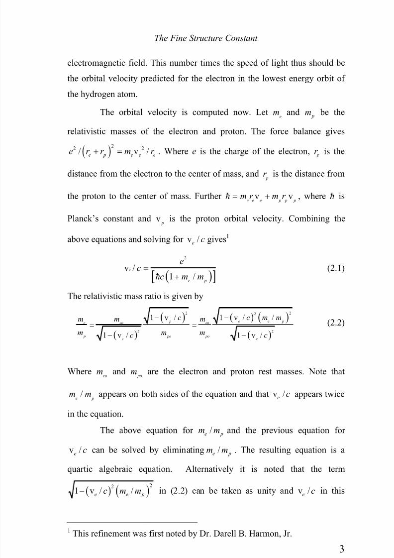
The orbital velocity is computed now. Lete
m and p
m be the
relativistic masses of the electron and proton. The force balance gives
( )22 2/ v /
e p e e ee r r m r + = . Where e is the charge of the electron,
er is the
distance from the electron to the center of mass, and pr is the distance from
the proton to the center of mass. Further v ve e e p p pm r m r = + , where is
Planck’s constant and v p
is the proton orbital velocity. Combining the
above equations and solving for v /e
c gives1
( )[ ]
2
v /1 /
e
e p
ec
c m m=
+
(2.1)
The relativistic mass ratio is given by
( )
( ) ( ) ( )
( )
2 22
2 2
1 v / 1 v / /
1 v / 1 v /
p e e pe eo eo
p po poe e
c c m mm m m
m m mc c
− −= =
− −
(2.2)
Whereeo
m and po
m are the electron and proton rest masses. Note that
/e pm m appears on both sides of the equation and that v /e c appears twice
in the equation.
The above equation for /e p
m m and the previous equation for
v /e
c can be solved by eliminating /e pm m . The resulting equation is a
quartic algebraic equation. Alternatively it is noted that the term
( ) ( )2
21 v / /e e pc m m− in (2.2) can be taken as unity and v /e c in this
1 This refinement was first noted by Dr. Darell B. Harmon, Jr.
7/30/2019 The Grand Unified-mobilecrackers
http://slidepdf.com/reader/full/the-grand-unified-mobilecrackers 10/143
Grand Unified Theory of Physics
4
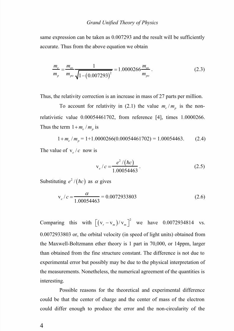
same expression can be taken as 0.007293 and the result will be sufficiently
accurate. Thus from the above equation we obtain
( )2
11.0000266
1 0.007293
e eo eo
p po po
m m m
m m m= =
−. (2.3)
Thus, the relativity correction is an increase in mass of 27 parts per million.
To account for relativity in (2.1) the value /e pm m is the non-
relativistic value 0.00054461702, from reference [4], times 1.0000266.
Thus the term 1 /e pm m+ is
1 /e pm m+ = 1+1.0000266(0.00054461702) = 1.00054463. (2.4)
The value of v /ec now is
( )2 /v /
1.00054463e
e cc =
. (2.5)
Substituting ( )2 /e c as α gives
v /1.00054463
ec
α = = 0.0072933803 (2.6)
Comparing this with ( )2
v v / vr m m−⎡ ⎤⎣ ⎦ we have 0.0072934814 vs.
0.0072933803 or, the orbital velocity (in speed of light units) obtained from
the Maxwell-Boltzmann ether theory is 1 part in 70,000, or 14ppm, larger
than obtained from the fine structure constant. The difference is not due to
experimental error but possibly may be due to the physical interpretation of
the measurements. Nonetheless, the numerical agreement of the quantities is
interesting.
Possible reasons for the theoretical and experimental difference
could be that the center of charge and the center of mass of the electron
could differ enough to produce the error and the non-circularity of the
7/30/2019 The Grand Unified-mobilecrackers
http://slidepdf.com/reader/full/the-grand-unified-mobilecrackers 11/143
The Fine Structure Constant
5
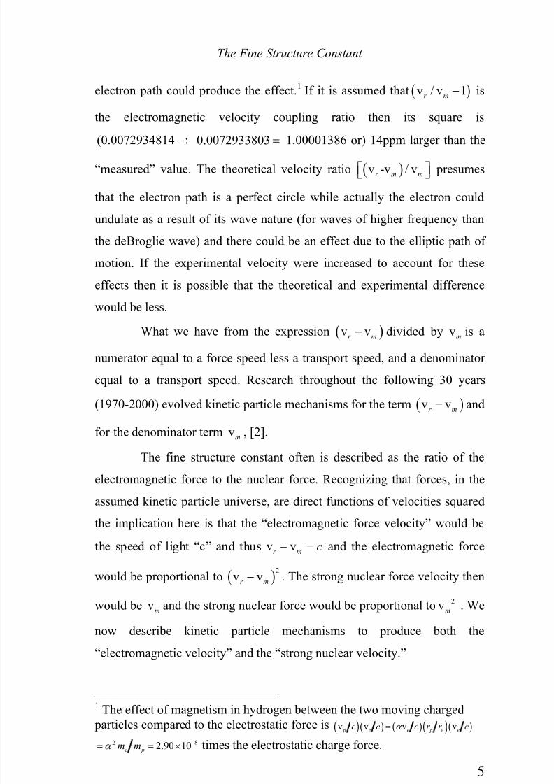
electron path could produce the effect.1 If it is assumed that ( )v / v 1r m − is
the electromagnetic velocity coupling ratio then its square is
(0.0072934814 0.0072933803÷ = 1.00001386 or) 14ppm larger than the
“measured” value. The theoretical velocity ratio ( )v -v / vr m m⎡ ⎤⎣ ⎦ presumes
that the electron path is a perfect circle while actually the electron could
undulate as a result of its wave nature (for waves of higher frequency than
the deBroglie wave) and there could be an effect due to the elliptic path of
motion. If the experimental velocity were increased to account for these
effects then it is possible that the theoretical and experimental difference
would be less.
What we have from the expression ( )v vr m
− divided by vm
is a
numerator equal to a force speed less a transport speed, and a denominator
equal to a transport speed. Research throughout the following 30 years
(1970-2000) evolved kinetic particle mechanisms for the term
( )v v
r m
− and
for the denominator term vm
, [2].
The fine structure constant often is described as the ratio of the
electromagnetic force to the nuclear force. Recognizing that forces, in the
assumed kinetic particle universe, are direct functions of velocities squared
the implication here is that the “electromagnetic force velocity” would be
the speed of light “c” and thus v vr m c− = and the electromagnetic force
would be proportional to ( )2
v vr m− . The strong nuclear force velocity then
would be vmand the strong nuclear force would be proportional to 2v
m. We
now describe kinetic particle mechanisms to produce both the
“electromagnetic velocity” and the “strong nuclear velocity.”
1 The effect of magnetism in hydrogen between the two moving charged particles compared to the electrostatic force is ( ) ( ) ( )( )( )v v v v p e e p e ec c c r r cα =
2 82.90 10e pm mα −= = × times the electrostatic charge force.
7/30/2019 The Grand Unified-mobilecrackers
http://slidepdf.com/reader/full/the-grand-unified-mobilecrackers 12/143
Grand Unified Theory of Physics
6
In order to have observable phenomena in a hard particle ether
universe it is necessary to have a basic organizing mechanism. As a prelude
to describing an organizing mechanism let us first describe a relateddisorganizing phenomenon.
Consider a perfectly elastic cubic box containing a gas of N
identical elastic spheres of mass “m” uniformly distributed throughout the
box. All have exactly the same speed “v”. Further, initially N 1 6 of these
particles move to the right, N 1 6 move to the left, N 1 6 move upward,
N 1 6 move downward, N 1 6 move inward, and N 1 6 move outward. The
initial mean speed, of course, is “v”. The initial root mean square speed also
is “v”, since all speeds are the same. Without any interference the particles
will collide and take a Maxwell-Boltzmann speed distribution. The initial
energy is ( ) 21/ 2 N vm and the final energy is ( ) 21/ 2 N vm . Thus
v v ' vr r
= = , where the prime indicates the final condition. The initial
linear momentum is zero. However, in a Maxwell-Boltzmann distribution
the mean speed is given in terms of the root mean square speed by
( )v 8 / 3 v 0.92vm r r
π = = . The mean speed dropped by 8 percent in this
process.
We will now describe a possible organizing mechanism, again see
Chapter 5 and Appendix B. Consider a tornado-like flow of the gaseous
particles which has rotation coupled with a sink-source flow. The rotation
of some assemblages would be right-handed and the rest would be left-
handed. Assume that the inflow to the sink is a gas that becomes completely
“condensed” so that the particles are touching each other to produce a solid
moving core translating and rotating like a rifle bullet and the particle
speeds, just before the final condensation, are an unchanged (speed) random
sample of the Maxwell-Botlzmann distributed background, and that the
7/30/2019 The Grand Unified-mobilecrackers
http://slidepdf.com/reader/full/the-grand-unified-mobilecrackers 13/143
The Fine Structure Constant
7
inflow to this condensed “core” is axial along the doublet axis.1 The particle
inflow velocity will then be vm , the background mean speed. The particle
inflow energy will be proportional to 2vr , the square of the background
root mean square velocity. Consider an imaginary cylindrical tube defining
the condensed core. If energy is conserved during this final condensation
process the flow velocity must increase from vm to v r , the opposite of the
disorganizing process described above. Thus, an axial thrusting force must
be occurring on the side of the condensed core which is proportional
to ( )2
v vr m− .
This thrust propels the assemblage. The assemblage has inflow into
the core at velocity vm , an outflow at velocity vr , and the outflow
circulates via the doublet flow back to the inlet. The whole assemblage
moves at the velocity vr - vm . All observables in the universe are assumed
to be made up of these assemblages so all observed phenomena are due toassemblages moving at the speed of light. The assemblages presumably are
formed with a range of masses, which mass is all in the core. The core is all
contained within a sphere with a diameter of one mean free path. The
angular momentum and thrust presumably are dependent only upon the
1 The size of the condensed core is estimated by assuming essentially a radial constant density
inflow to a sphere with a radius equal to the mean free path , l , at which radius the gas reachesthe background mean speed vm . Independent of the shape of stream tubes inside this mean
free path radius if the flow is assumed spherically symmetric, there is a spherical space where
the gas is completely condensed (i.e. all particles are touching others). The mass inflow rate m
at the mean free path sphere is ( ) 2
v v 4 .b m
a m l ρ η π = The mass inflow at the condensed sphere
radius is 2 2
mv 4 3 v 4 .b b va m r r ρ π π ⎡ ⎤= ⎣ ⎦ In these expressionsbm is the basic particle mass
( )66
10 kg −
,b
r is the particle radius ( )35
10 m− ,η is the background particle number density
( )85 3
10 m , and vr is the core sphere radius. Solving this gives 262 10vr m−× . This is a rough
estimate of the minimum size core, its mass is
( ) ( ) ( )3
3 3 26 35 66 384/3 4/3 2 10 10 10 10 .v v b bm r r m kg π π
− − − −= = × ×⎡ ⎤
⎣ ⎦
7/30/2019 The Grand Unified-mobilecrackers
http://slidepdf.com/reader/full/the-grand-unified-mobilecrackers 14/143
Grand Unified Theory of Physics
8
free-field properties and therefore do not vary with the core mass. As the
condensation begins to take place by background particles flowing into a
sink the particles can almost reach sonic speed by flowing inward alongstraight stream tubes. After reaching this speed it is necessary for the stream
tubes to curve. Curved stream tubes produce thermal velocity separation of
the particles because of the centrifugal force on the particles. Such thermal
separation occurs in Ranque-Hilsch vortex tubes, see Lay [5]. This thermal
separation due to inertia may be a part of the mechanism which permits
complete condensation of a gas. In any case, going down a curved path
causes rotation and thus produces angular momentum. Such an assemblage
as envisioned here produces an angular momentum depending only upon
the mean free path and other background ether properties, thus causing all
observable elements to have the one constant value of angular momentum.
In order for such an assemblage as envisioned to occur it almost
certainly must be contained principally within a region extending a distance
in the order of the mean free path “l ”. If the structure were much larger than
one mean free path the assemblage would be disrupted by the outflow.
Consistent with this requirement we assume that the inflow is radial down
to the surface of a sphere with a radius equal the mean free path and, at that
location, the flow velocity is vm . Actually, the stream tubes will be curving
by then, but for our analysis we will assume all the rotatory component has
been achieved by an average radius of 0.8l . Further, we assume the time the
mass is inside the mean free path radius sphere is for a length of l π divided
by vm. Now, the angular momentum of the assemblage is the flowing mass
inside the sphere, which is ( )( )2
0 4 v vm ml l ρ π π times its effective radius
0.8l times its velocity vm . Thus
( )( )( )24 v v 0.8 v02
l l l m m m ρ π π = (2.7)
or
7/30/2019 The Grand Unified-mobilecrackers
http://slidepdf.com/reader/full/the-grand-unified-mobilecrackers 15/143
The Fine Structure Constant
9
2 4
06.4 vml π ρ = (2.8)
The values of all these parameters are developed in Appendix A.
Substituting the values in (2.8) gives
( )( )( )4
2 19 9 176.4 1.0495 10 3.5103 10 8.2045 10π −= × × × (2.9)
34 21.0544 10 kg m s−= ×
This agrees closely with the measured value, of course, since we used this
equation to determine l , see Appendix A.
One specific value of core mass for an assemblage moving at the
speed of light in a circular path can produce an angular momentum of
/ 2 and have the centrifugal force balance the thrust. This particle would
model a proton. The value of this thrust is quite large – and can easily be
computed. The balance of centrifugal force with the thrust F is
2
p p F m c r = and the proton angular momentum is 2 p pm cr = .
Substituting pr from the angular momentum equation into the force
equation gives
2 3 27 2 3 342 2(1.67262158 10 ) (299792458) 1.054571596 10 p F m c − −= = × ÷ ×
(2.10)
61.42959 10 N = ×
This is a very large force!!
The orbiting assemblage, with a tangential speed vr - vm ( ,c= of
course,) produces two fields. One field is due to the continuous inflow at
velocity vm into the core sink (which is moving in a circular path at velocity
vr - vm
). Another field is the similar outflow translating at velocity vr from
the core source (moving at vr - vm ). The orbiting flow of the basic
assemblage produces the magnetic moment.
A flow meter, in principle, could move around fixed to the orbiting
assemblage at such a location that it always experienced an inflow at the
7/30/2019 The Grand Unified-mobilecrackers
http://slidepdf.com/reader/full/the-grand-unified-mobilecrackers 16/143
Grand Unified Theory of Physics
10
maximum speed vm . This field associated with this inflow is the strong
nuclear force field. At a distance “r” of many assemblage circular path
diameters a flow meter fixed with respect to the matter particle would
experience principally a spherically symmetric flow field which is
oscillating inward at velocity vmand outward at velocity amplitude vr
, the
source output velocity. Thus the field is an alternating flow of velocity
amplitude vr - vm . This field is the electromagnetic field.
In order to understand the particle interactions resulting from the
above described flow fields, let us review some experimental and
theoretical work on particles immersed in a medium. The following results
are taken from Whittaker [6].
In 1876, C.A. Bjerknes immersed two identical spheres in water,
had them oscillate in a breathing mode, and measured the mutual force of
interaction between the spheres. The force was found to be an inverse
square force, as expected, and it was attraction when the oscillation was in- phase and repulsion when out-of-phase. A theoretical analysis was
developed which explained the results. This analysis is presented in the
book by Bassett [10] and is repeated in Appendix C. Further, the theoretical
results were extended to gaseous media and to a large variety of oscillation
producing devices – all with the inverse square force result.
Now, consider the long-range force between two charged nucleons
(say a proton and proton, or proton and anti-proton). The basic assemblage
(i.e., the neutrino) producing the proton has rotation of one handedness and
the anti-proton has rotation with the opposite handedness. It is assumed that
like rotations would result in out-of-phase waves and unlike rotations would
result in in-phase waves, to give repulsion of like charges and attraction of
unlike charges respectively. The field strength would be measured by an
oscillating flow field of velocity vr - vm
. This spherically symmetric
oscillating flow field is the mechanism producing the electromagnetic force.
7/30/2019 The Grand Unified-mobilecrackers
http://slidepdf.com/reader/full/the-grand-unified-mobilecrackers 17/143
The Fine Structure Constant
11
Two nucleons at short range could have their assemblage circular
paths oriented and phased in such a way that they would experience only
the inflow at velocity varying from 0 to vm (and avoid the outflow velocity
vr ). The nuclear force strength then is proportional to 2v
m. This is the
strong nuclear force mechanism.
In the above envisioned universe the strongest possible attractive
force is produced by a flow velocity vm . The coupling velocity is vm , the
coupling force constant is unity for nuclear forces. For the electromagnetic
force the coupling velocity is vr - vm , the coupling velocity constant is
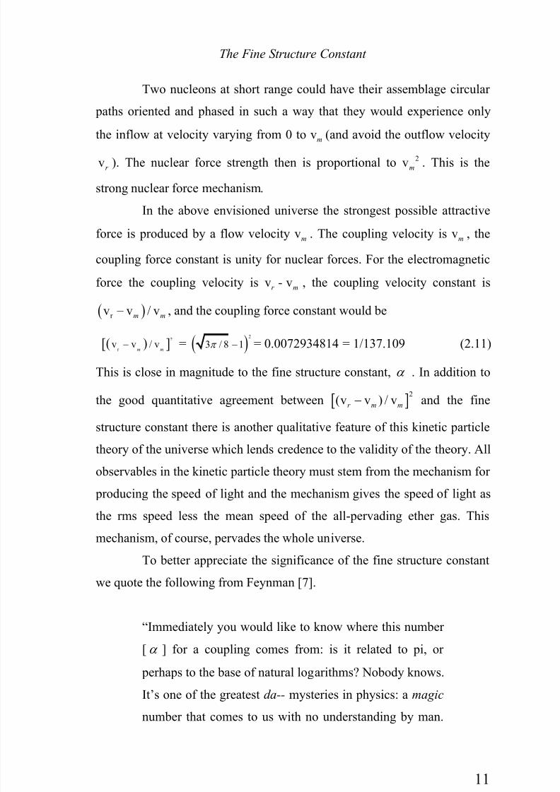
( )r v v / vm m− , and the coupling force constant would be
( )[ ]2
r v v / v
m m− = ( )
2
3 / 8 1π − = 0.0072934814 = 1/137.109 (2.11)
This is close in magnitude to the fine structure constant, α . In addition to
the good quantitative agreement between [ ]2
(v v ) / vr m m− and the fine
structure constant there is another qualitative feature of this kinetic particle
theory of the universe which lends credence to the validity of the theory. All
observables in the kinetic particle theory must stem from the mechanism for
producing the speed of light and the mechanism gives the speed of light as
the rms speed less the mean speed of the all-pervading ether gas. This
mechanism, of course, pervades the whole universe.
To better appreciate the significance of the fine structure constant
we quote the following from Feynman [7].
“Immediately you would like to know where this number
[ α ] for a coupling comes from: is it related to pi, or
perhaps to the base of natural logarithms? Nobody knows.
It’s one of the greatest da-- mysteries in physics: a magic
number that comes to us with no understanding by man.

7/30/2019 The Grand Unified-mobilecrackers
http://slidepdf.com/reader/full/the-grand-unified-mobilecrackers 18/143
Grand Unified Theory of Physics
12
You might say the “hand of God” wrote the number, and
‘we don’t know how He pushed His pencil’.”
The significance of the fine structure constant also is discussed by Lévy-
Leblond [8]. We believe the agreement of the Maxwell-Boltzmann derived
number and the fine structure number can not be dismissed as chance. The
kinetic particle theory of the universe must mirror reality.
7/30/2019 The Grand Unified-mobilecrackers
http://slidepdf.com/reader/full/the-grand-unified-mobilecrackers 19/143
Grand Unified Theory of Physics
13
3. Relativity and the Wave Property of Matter
In this book we have assumed a universe of identical elastic
spherical particles which particles make up a gaseous ether and make up all
matter and radiation. Further, we assume the gaseous ether is in a three
dimensional space with a separate absolute time. The particles are very
small with a diameter in the order of the Planck length ( )3510 m
− and with
a mass billions and billions times smaller than the electron. The particle
number density is very large ( )85 310 m
− and the mean free path is on the
order of nuclear particle diameters.
A photon is assumed to be a stable assemblage of a large number
of these ether particles translating at the speed of light, of course. Each
fundamental matter particle at rest such as a proton, is assumed to be a
neutrino which is a very small stable assemblage (again made up of very
many basic particles) moving at the speed of light in a circular path with a
very small diameter.
From these above assumptions we immediately have the result that
the energy of a matter particle at rest is the matter particle mass 0M (which
is the background particle mass times the number of particles making up the
matter particle) times the square of the speed of light. Defining energy as
mass times the square of the mass’s velocity then
0 0c² E M = (3.1)
which is the famous Einstein formula for the “equivalence” of mass and
energy.
In order to accelerate matter a series of photons bombard the
matter and each photon is partly scattered and partly captured. 1 The
captured parts of the photons are the mass that is added to the matter to
1 This process involves absorbing the impacting photon and then emitting alower energy photon.

7/30/2019 The Grand Unified-mobilecrackers
http://slidepdf.com/reader/full/the-grand-unified-mobilecrackers 20/143
Grand Unified Theory of Physics
14
accelerate it. When a force does work on a particle of mass m and
accelerates m from zero velocity to v, the work done is ½ m v² so that
½ m v² is the particle’s kinetic energy change. If a mass moving at velocity
v (having energy 2vm ) is absorbed by another mass moving at the same
magnitude and direction of velocity v then the energy change of the
increased mass particle is m v². Consider now a photon of energy c²e mγ γ
= .
This can be written in terms of its linear momentum pγ
as 2( / )e p c cγ γ = .
Consider the acceleration of a matter particle due to the result of scattering
photons. Leto be the mass of the matter particle at rest and let v be the
mass when moving at velocity v . The matter particle energy when moving
is 2
vc and the linear momentum is v vm P M = . The linear momentum
P γ
of the photons (assuming many photons were used) is P M cγ γ = , where
γ is the sum of the photon “masses”. Let the scattered photon total
“mass” be s kM γ = so that the captured “mass” is (1 )c k M γ = − . The
momentum transferred by the captured mass of each photon is (1 )m k cγ − ,
where mγ
is the “mass” of one photon. The momentum transferred by the
scattered portion of each photon is m kcγ
, since the scattering is spherically
symmetric with the maximum back scatter momentum being 2m kcγ
and
the minimum forward scatter is zero for an average of m kcγ
. Thus, the
momentum transferred to the matter particle is all of each photon’s
momentum. The total momentum imparted then is the sum of the initial
momentum of each photon. Let us denote the total momentum as P . The
differential energy change for the matter particle is the force times the
distance so
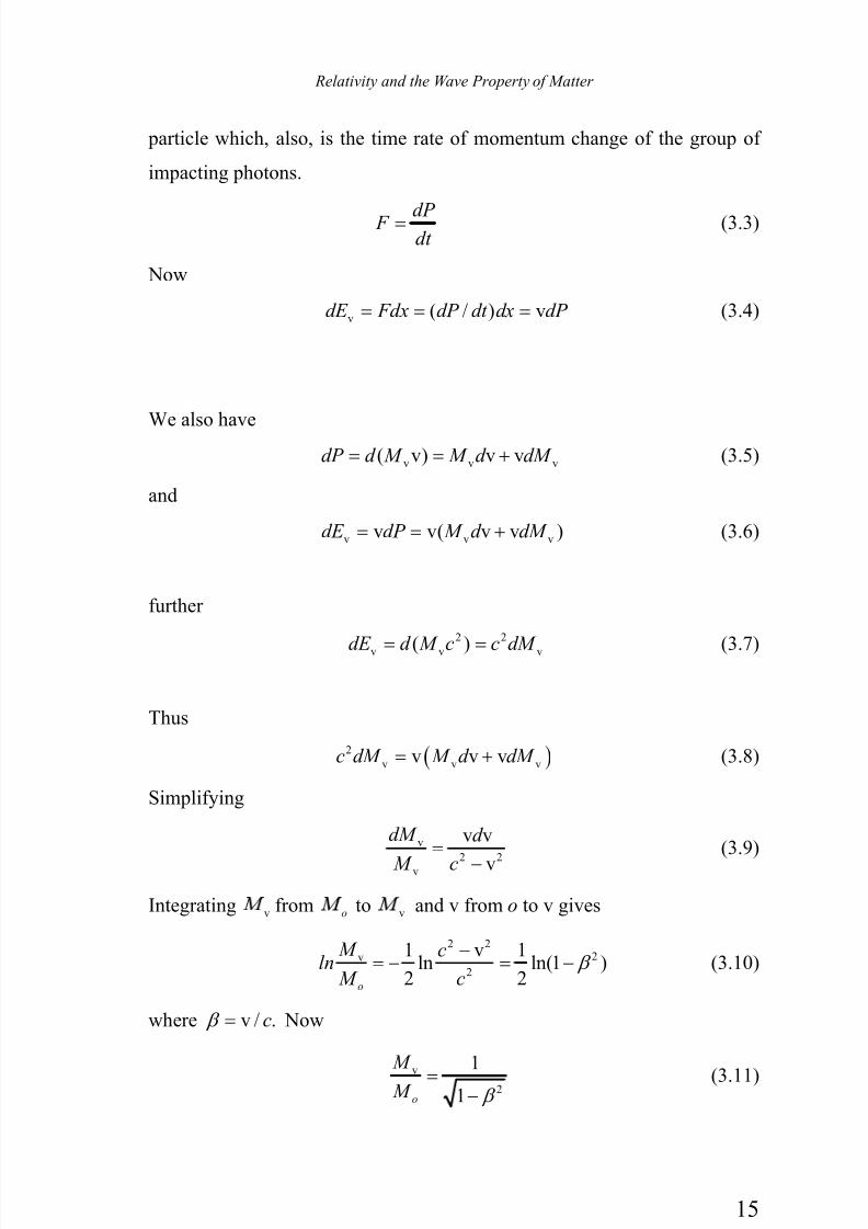
vdE Fdx= (3.2)
where E v is the energy of the moving matter particle and F is the force
applied. The force is the time rate of momentum change of the matter
7/30/2019 The Grand Unified-mobilecrackers
http://slidepdf.com/reader/full/the-grand-unified-mobilecrackers 21/143
Relativity and the Wave Property of Matter
15
particle which, also, is the time rate of momentum change of the group of
impacting photons.
dP F dt
= (3.3)
Now
v ( / ) vdE Fdx dP dt dx dP = = = (3.4)
We also have
v v v( v) v vdP d M M d dM = = + (3.5)
and
v v vv v( v v )dE dP M d dM = = + (3.6)
further
2 2
v v v( )dE d M c c dM = = (3.7)
Thus
( )2
v v vv v vc dM M d dM = + (3.8)
Simplifying
v
2 2v
v v
v
dM d
M c=
−
(3.9)
Integrating v from o to v and v from o to v gives
2 22v
2
1 v 1ln ln(1 )
2 2o
M cln
M c β
−= − = − (3.10)
where v / .c β = Now
v
2
1
1o
M
M β = −(3.11)

7/30/2019 The Grand Unified-mobilecrackers
http://slidepdf.com/reader/full/the-grand-unified-mobilecrackers 22/143
Grand Unified Theory of Physics
16
We see that this is the well known mass growth equation and note it has
been derived from classical Newtonian mechanics which uses an absolute
space with a separate absolute time system.
1
Let us determine the portion of the photon mass that is captured and that
which is scattered. The captured mass is
( )2 2
v 0 0 1 1 1c M M M M β β = − = − − − (3.12)
The momentum balance relates the scattered and captured mass by the
equation2
0( ) ( )v s c c M M c M M + = + (3.13)
Thus
( ) 2 2
0 0 1 1 1 s c c M M M M M β β β β ⎡ ⎤= + − = − + − ÷ −⎣ ⎦
(3.14)
Now
( )21 1 1 s c M M β β = − − − ( )21 1 1 s c M M β β = − − − (3.15)
Some values of / s c M versus β are now obtained.
β 0.01 0.02 0.1 0.5 0.8 0.9 0.99
/ s cm m 199 99.0 18.9 2.73 1.0 0.595 0.153
From this table we note that at small velocities practically all the mass is
scattered, while at large velocities practically all the mass is captured.
The fact that the velocity of matter can never exceed the speed of
light results simply from the fact that the accelerating agent (i.e. the photon)
is moving at the speed of light.
When a photon interacts with matter at rest the circular path becomes a
spiral path as seen from a rest frame. However, in a frame moving at the
translational velocity v of the particle the spiral is seen as a closed path and
1 This analysis was developed for this theory by Dr. Darell B. Harmon, Jr.2 This results since the average scattered mass has its velocity at 90° to theimpacting velocity.
7/30/2019 The Grand Unified-mobilecrackers
http://slidepdf.com/reader/full/the-grand-unified-mobilecrackers 23/143
Relativity and the Wave Property of Matter
17
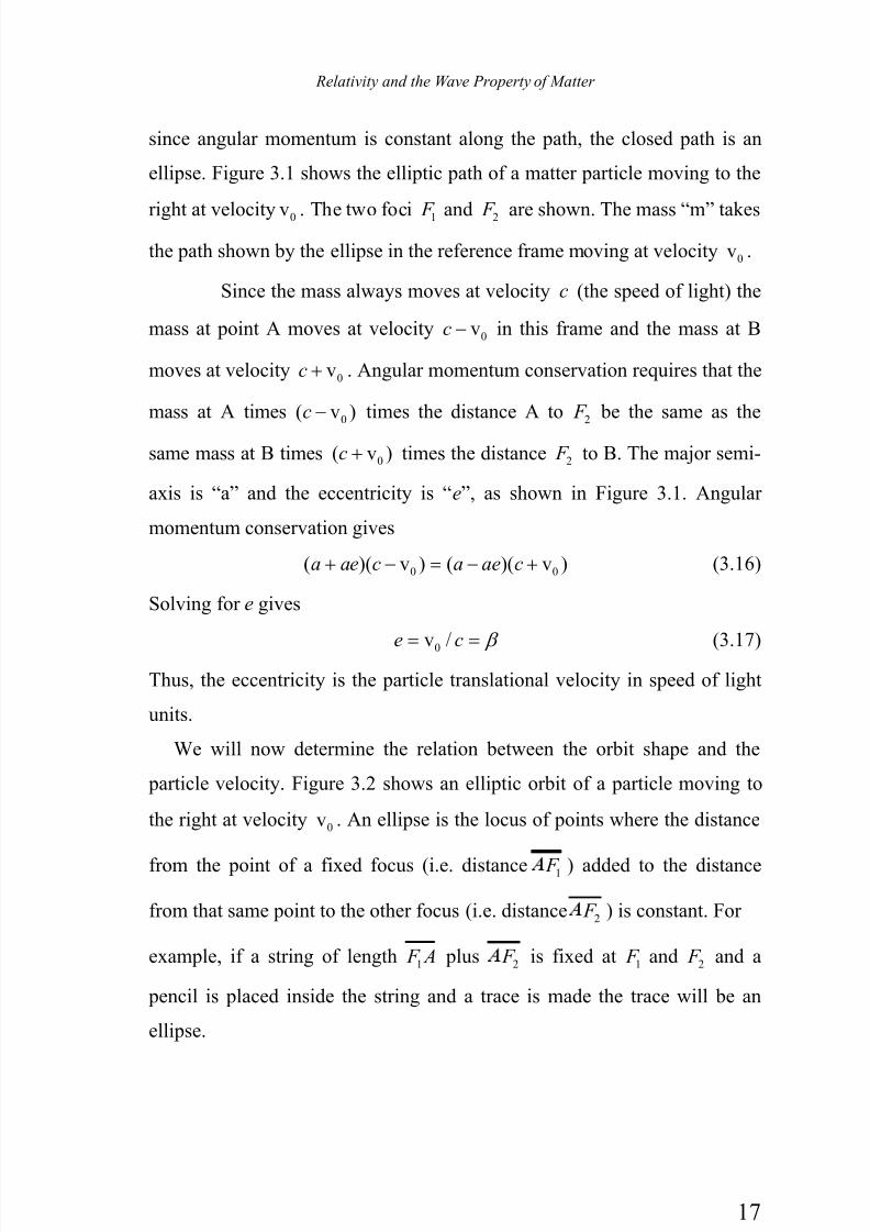
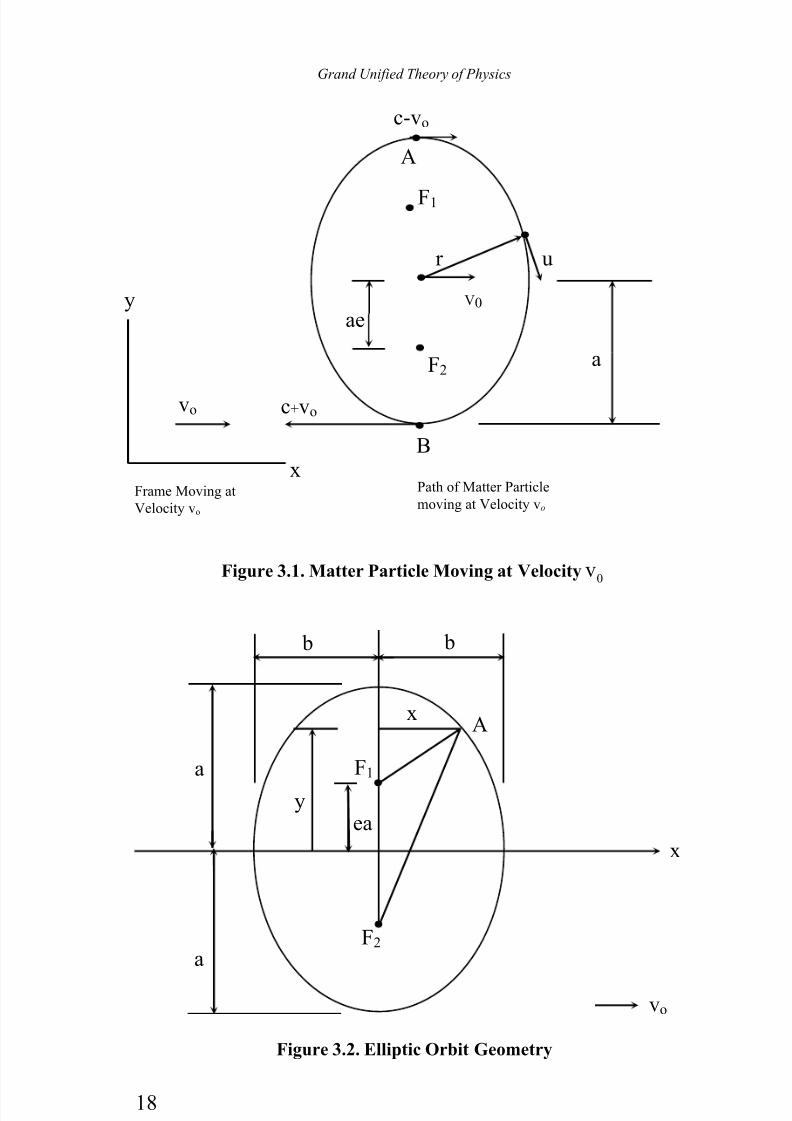
since angular momentum is constant along the path, the closed path is an
ellipse. Figure 3.1 shows the elliptic path of a matter particle moving to the
right at velocity 0v . The two foci 1 F and 2 F are shown. The mass “m” takes
the path shown by the ellipse in the reference frame moving at velocity 0v .
Since the mass always moves at velocity c (the speed of light) the
mass at point A moves at velocity 0vc − in this frame and the mass at B
moves at velocity 0vc + . Angular momentum conservation requires that the
mass at A times 0( v )c − times the distance A to 2 F be the same as the
same mass at B times 0( v )c + times the distance 2 F to B. The major semi-
axis is “a” and the eccentricity is “e”, as shown in Figure 3.1. Angular
momentum conservation gives
0 0( )( v ) ( )( v )a ae c a ae c+ − = − + (3.16)
Solving for e gives
0v /e c β = = (3.17)
Thus, the eccentricity is the particle translational velocity in speed of light
units.
We will now determine the relation between the orbit shape and the
particle velocity. Figure 3.2 shows an elliptic orbit of a particle moving to
the right at velocity 0v . An ellipse is the locus of points where the distance
from the point of a fixed focus (i.e. distance 1 F ) added to the distance
from that same point to the other focus (i.e. distance 2 F ) is constant. For
example, if a string of length 1 F A plus 2 F is fixed at 1 F and 2 F and a
pencil is placed inside the string and a trace is made the trace will be an
ellipse.
7/30/2019 The Grand Unified-mobilecrackers
http://slidepdf.com/reader/full/the-grand-unified-mobilecrackers 24/143
Grand Unified Theory of Physics
18
Figure 3.1. Matter Particle Moving at Velocity 0v
Figure 3.2. Elliptic Orbit Geometry
b b
xA
F1
F2 a
a
yea
x
vo
F1
c-vo
A
ae
a
r
vo c+vo
F2
V0
u
B
y
xFrame Moving at
Velocity vo
Path of Matter Particle
moving at Velocity vo
7/30/2019 The Grand Unified-mobilecrackers
http://slidepdf.com/reader/full/the-grand-unified-mobilecrackers 25/143
Relativity and the Wave Property of Matter
19
The length of the string is given by
2 2 2 212 ( ) ( ) 2 F A AF ea y x y ea x a+ = + + + − + = (3.18)
which simplifies to
2 2 2 2 2 2 2( )( )a a e a y a x− − = (3.19)
or
2 2 2 2(1 )( )e a y x− − = (3.20)
when
y = 0 x = ± b (3.21)
then
2 2 2(1 )a e b− = (3.22)
Thus
2/ 1b a e= − (3.23)
Since e = 0v / c β =
, from (3.23), we have2/ 1b a β = − (3.24)
This is the ratio of the minor axis to the major axis and clearly shows the
orbit size reduction. Every matter particle in a piece of matter, such as a bar
of steel, experiences this shortening with velocity. Thus, the complete bar
will be shortened in the direction of motion by the factor 21 β − . We
therefore have
2
v 1ol l β = − (3.25)
The velocity “u” of mass “m” on this elliptic path at radius r from 2 F , as
shown in Figure 3.1, is given in [9] by the equation
[ ]2 2 / 1/u g r a= − (3.26)
where “g” is a constant (=GM by McClusky in [9]). The maximum velocity
is when (1 )r a ea e a= − = − and has the value 0vc + . From this
7/30/2019 The Grand Unified-mobilecrackers
http://slidepdf.com/reader/full/the-grand-unified-mobilecrackers 26/143
Grand Unified Theory of Physics
20
2
0
2 1 1( v )
(1 ) 1
ec g
e a a a e
⎡ ⎤ ++ = − =⎢ ⎥− −⎣ ⎦
(3.27)
and2( v ) (1 ) /(1 )o
c a e e= + − + (3.28)
Let the time for an orbit, i.e. the period, be vτ (from [9]), substituting the
value of GM as g from the above, and using e as β gives
( )3/ 2 2
v 2 2 1a g a cτ π π β = = − (3.29)
When vo = 0 (i.e. when β = 0) the period = 2 /r cπ -- obviously
the circumference of the circle divided by the speed of light. The period
increases with motion and grows without bound as ( )0v / c β = approaches
unity, or as the velocity approaches the speed of light. Nuclear particles,
which disintegrate and emit radiation and produce other matter particles, are
observed to decay slower when moving – and governed by the law,
2
v 0/ 1/ 1τ τ β = − where vτ is the decay time while moving at velocity v
and 0τ is the decay time while at rest. If it is presumed that decay takes an
average number of orbits at rest and that the decay process depends upon
the number of orbits (i.e. the number of trials at breaking loose) then it
follows that
v 0/τ τ = 2
1/ 1 β − . (3.30)
This gives the time dilation effect produced by the special theory of
relativity but here derived from a classical Newtonian basis.
When any matter particle translates from one place to another
along a nominal straight path, it always undulates from one side to the other
as it moves. All matter at rest consists of elementary matter particles which
consist of mass moving at the speed of light in circular paths. Ordinarymatter, such as a bar of steel, is accelerated from rest by photons being
transferred, usually from other matter (such as during impact by another
bar). In the previous paragraphs we discussed how these photons interact
7/30/2019 The Grand Unified-mobilecrackers
http://slidepdf.com/reader/full/the-grand-unified-mobilecrackers 27/143
Relativity and the Wave Property of Matter
21
with the flow fields produced by matter to accelerate the matter particles.
When a small (low energy-long wavelength) photon interacts with a matter
particle the distance from the particle center of mass to the coupling position must be in the order of the wavelength of the photon. Angular
momentum considerations require that small impacts be at large distances
from the center of the matter particles. Thus, the smaller the interacting
photon energy (and the longer the wavelength) and the smaller the resulting
matter particle velocity the greater the eccentricity of the coupled mass.
Now consider a free wheel in space rotating with a small unbalanced mass
placed at a large radius. The axis of the wheel will undulate as it translates
to keep the center of mass following an exact straight line. As a result the
center of the wheel will take a sinusoidal path to the left and right of the
center-of-mass straight path. Let us now calculate the wavelength of the
moving matter geometric center path.
Let cr be the distance from the matter particle’s center to the place
where the momentum is captured, by both the captured mass and scattered
mass. The linear momentum “ P ” times the capture radius is c Pr - which is
assumed to be . For low velocities (i.e. non-relativistic conditions) the
momentum P is also 0v M , where 0 is the matter particle rest mass. Now,
we can write
vc o c Pr M r = =
, 2 v2 vo c oh M r M π π λ = = =
(3.31)where λ is the wavelength. Thus
( )/ voh M h P λ = = (3.32)
This is the relation postulated by deBroglie and is called the “deBroglie
wavelength”. For high speeds (i.e. for relativistic speeds) consideration
must be given to matter particle mass growth, the center of gravity
difference, and the matter particle contribution to the angular momentum.
The wavelength λ is measured in meters, the constant h is 346 10−×
kilogram-meter 2
per second (i.e. Planck’s constant), 0 is the matter
7/30/2019 The Grand Unified-mobilecrackers
http://slidepdf.com/reader/full/the-grand-unified-mobilecrackers 28/143
Grand Unified Theory of Physics
22
particle rest mass in kilograms, and “v” is the particle translational velocity
in meters per second. An electron with a mass of 3010 kg − and a velocity
1/ 3 the speed of light (i.e., 810 /m s ) has a wavelength of
3412
30 8
6 106 10
10 10
x x
xλ
−−
−= = meters (3.33)
– a very small wavelength. The amplitude of the oscillation is much smaller
than the wave length.
The observation of high speed mass growth with velocity is a
significant part of high speed (relativity) physics and the observation of
matter moving as a wave is a significant part of small item (quantum)
physics. Both of these mechanisms come about simply from the interaction
of a photon with matter – as shown by the mass growth formula and the
wavelength formula just derived.
Throughout the 20th century many authors have stated the
impossibility of deriving the special relativity results from classical
(Newtonian) theory. We have shown that the three primary relativity
observations (mass growth, matter shortening, and time dilation) are derived
in a straightforward manner from a classical kinetic particle theory. Further,
the mass-energy equivalence 2
0 E M c= is an obvious result of the theory.
Finally, we have derived the wave properties of matter rather than
postulating them – as done in contemporary physical theory. In summary,
these results indicate that the universe is a classical based system.
7/30/2019 The Grand Unified-mobilecrackers
http://slidepdf.com/reader/full/the-grand-unified-mobilecrackers 29/143
Electrostatics and Magnetism
23
4. Electrostatics and Magnetism
In this Newtonian universe of hard particles making up an ether,
the assemblages of these particles (i.e., neutrinos) orbiting at the speed of
light in circular orbits make up all matter at rest. The assemblages making
up matter all have angular momentum which is either right-handed or left-
handed. The different handedness makes the difference between positive
and negative electrostatic charge.
The orbiting assemblage making up a charged particle produces a pulsation in the ether like that of a breathing sphere. Two such assemblages
whose centers are at a distance “ R” apart can produce an inverse square
force of interaction between them. The maximum magnitude of the force
produced is given by Bassett1 [10] as
2 2 2
0 2 2
8e
e
a b F
T R
π αβ ρ = (4.1)
This analysis of Bassett is reproduced as Appendix C. In this equation “a”
is the nominal radius of one breathing sphere (the proton orbital radius), “b”
is the nominal radius of the other, “ α ”is the half amplitude of oscillation
on one sphere which is taken as the proton orbital radius, “ β ” is the half
amplitude of the other sphere, eT is the period of charge oscillation, 0 ρ is
the background mass density, and R is the separation distance. For more background see Whittaker [6]. With electrostatic charges all charges are
alike except for the sign which, in this kinetic particle theory here, is
controlled by the direction of rotation of the charge-producing assemblage
(i.e., the neutrino) about its orbital tangential velocity. Thus, we set b=a and
a β α = = so that
1 In Bassett the background density is taken as unity and does not appear inthe formula.
7/30/2019 The Grand Unified-mobilecrackers
http://slidepdf.com/reader/full/the-grand-unified-mobilecrackers 30/143
Grand Unified Theory of Physics
24
2 6
2 2
8e o
e
a F
T R
π ρ = (4.2)
The period of oscillation is
2 /eT a cπ = (4.3)
Now
4 2
2
2e o
a c F
R ρ = (4.4)
Since (4.4) gives the electrostatic force, the force also is2 2
e R so
that
2
02e a c ρ = (4.5)
and using “a” as pr we have (from Appendix A)
( ) ( ) ( )2
2 19 16 8
02 2 1.0495 10 1.0516 10 2.9979 10 pe r c ρ −= = × × × (4.6)
14 1 2 3 2 1
1.5189 10 kg m s− −
= ×
Which agrees with the measured value, as it must since the measured value
of “e” was used to determine the basic constants.
Let us now determine the effect of motion on the electromagnetic
force between two charged particles. An electron at rest, in the assumed
kinetic particle universe, has an assemblage of kinetic particles orbiting at
the speed of light in a circular path. In order to accelerate an electron a photon with angular momentum “ ” “impacts” the electron electrostatic
field. The angular momentum of the combined assemblage (consisting of
the electron and the captured portion of the photon) increases by and the
two entities combined translate at velocity “v”. The angular momentum
then of the combined entities is vcmr = , where m is the mass (of the two
entities) and “r c” is the half-amplitude of the center of the “charge”. The
center of mass, of course, continues on a straight path. The undulation of
the center of charge is the “electron wave”.

7/30/2019 The Grand Unified-mobilecrackers
http://slidepdf.com/reader/full/the-grand-unified-mobilecrackers 31/143
Electrostatics and Magnetism
25
Consider now two like electric charges moving at velocity v
parallel to each other and with a vector R starting at one charge and ending
at the other and which vector is perpendicular to the particle velocities. In areference frame moving at velocity “v” the two charges are seen to oscillate
along the vector v. Assuming phasing is controlled by the twist component
of the orbiting assemblage producing the charged particle, the maximum
force of interaction between the two particles is given by the same form as
the formulas for electrostatic charge, again see [2] and [6]. The difference is
that a will be the deBroglie wave amplitude of the charge (which
is ( )/ 2λ π ), and the period T m will be / vλ . The force then due to motion
will be
( )( )( )
22 42 4 2 4 2
0 0 02 2 2 22
8 / 28 2 v
/ vm
m
aa a F
T R R R
π λ π π α ρ ρ ρ
λ = = = (4.7)
Dividing the magnetic force by the electrostatic force gives2
2
vm
e
F
F c= (4.8)
for the special case of equal charges, equal and parallel velocities, and a
charge separation vector initiating on one charge and ending on the other
where the vector is perpendicular to both velocities. This ratio, of course, is
the ratio of the magnetic force to the electrostatic force for this special case.Thus this mechanism models the magnetic force.
If the charges have the same sign then the force is attractive, if
opposite, the force is repulsive. By the same mechanism, for which an
understanding has not been developed, if the charge velocities are opposite
the repulsion/attraction is reversed.
Let us now generalize the special case just developed. Consider a
velocity 1v , of charge 1 which produces 100 oscillations in a given period of
time. Starting with velocity 2v , of charge 2 with 100 oscillations, if the
7/30/2019 The Grand Unified-mobilecrackers
http://slidepdf.com/reader/full/the-grand-unified-mobilecrackers 32/143
Grand Unified Theory of Physics
26
velocity is reduced say to 1 oscillation in the same time period then the
force, clearly, would be reduced to 1/100th of the initial value. Thus, we can
generalize the magnetic force equation to2
1 2
2
v vm
e F
c c R
⎛ ⎞⎛ ⎞= ⎜ ⎟⎜ ⎟
⎝ ⎠⎝ ⎠(4.9)
where 1v and 2v can be any value, negative or positive.
The next generalization is for unlike charge magnitudes. We let
1 N be the number of elementary charges at one location and 2 N at the other
and take
1 1q N e= and 2 2q N e= (4.10)
then
1 2 1 2
2
v vm
q q F
c c R
⎛ ⎞⎛ ⎞= ⎜ ⎟⎜ ⎟
⎝ ⎠⎝ ⎠(4.11)
If 1v and 2v are perpendicular to each other then the force would
be zero because of the phasing and should vary sinusoidally from zero when
perpendicular to a maximum magnitude when parallel (or anti-parallel).
Finally, if the radius vector R for the general case starts at charge 1
and ends at charge 2 (no matter what the relative locations and directions
that the charges have) we have the magnetic force given by
1 2 1 22 1 2 12 2 2 2
v v v v Rm R
q q i q q F i
c R c R
= × × = × ×
(4.12)
In this expression 1q and 2q are the point charges with units of
1/ 2 3/ 2 1kg m s− , 1v and 2v are the charge velocities in m/s, Ri
is a unit vector
from charge 1 to charge 2, R is the magnitude in meters of the vector from
charge 1 to charge 2, c is the speed of light in m/s, and F m is the magnetic
force in newtons, which is attractive in the case where the velocities are
parallel and equal and the charges are of like sign.
7/30/2019 The Grand Unified-mobilecrackers
http://slidepdf.com/reader/full/the-grand-unified-mobilecrackers 33/143
7/30/2019 The Grand Unified-mobilecrackers
http://slidepdf.com/reader/full/the-grand-unified-mobilecrackers 34/143
Grand Unified Theory of Physics
28
since the particle velocities in this frame would be zero.
The particle response is experienced only by the acceleration and
in this moving frame it would by2 2
v/d y d τ , if the y-axis is taken to pass
through the two particles. The response then as measured by a clock at rest
would be
( )( ) ( )2 2 2
2 2
2 2 2
v 0 0
1 v / 1 v /d y d y d y
c cd d d τ τ τ
⎡ ⎤= − = −⎣ ⎦
(4.18)
Thus, the force would have to be reduced by the factor ( )2
1 v / c⎡ ⎤−⎣ ⎦
. If the
charges are of opposite sign then the electrostatic force is attractive but the
magnetic force is repulsive so that the same factor ( )2
1 v / c⎡ ⎤−⎣ ⎦
, results.

7/30/2019 The Grand Unified-mobilecrackers
http://slidepdf.com/reader/full/the-grand-unified-mobilecrackers 35/143
Neutrino, Proton, Electron, and Neutron Structures
29
5. Neutrino, Proton, Electron, and Neutron Structures
The basic assemblage of ether particles translates at the velocity
v vr m− , which is the speed of light, has a spin of 1 2 , and has a very small
cross section on the order of neutrino cross sections, and thus this
assemblage models the neutrinos. The single orbiting neutrino which has an
orbital angular momentum of 2 is the proton. The electron is formed
when the proton is formed and the electron’s formation implies a particular
triple-looped structure. Given this structure there is an implied structure for
the neutron, which we present. Let us now review the model of the proton
which the kinetic particle theory implies. The proton is a neutrino moving at
the speed of light in a circular orbit. The proton angular momentum is
2 p pm r c= -- from which the proton path radius pr is given by
( ) ( )34 272 1.0545716 10 2 1.672621 10 299792458 p pr m c− −= = × × × × (5.1)
161.051545 10−= ×
The electrostatic field is produced by the (small) assemblage acting as a ball
moving in this circular path – and has been given here previously. The
magnetic moment is produced by the circular traveling pulse flow in the
first few waves (of the electrostatic field) surrounding the sphere defining
the disturbance of the path of radius pr . To agree with the measured
magnetic moment this radius must be 2.79 pr -- which seems reasonable but
we have not been able to precisely calculate its value. The anti-proton is
formed from a translating assemblage with spin opposite that of the one
forming the proton.
Let us now discuss the strong nuclear force between two protons
(or nucleons). For the time being we will assume that the electrostaticfields of the two protons are non-existent. Of course, we are implying that
one of the protons is a neutron, but we will develop the neutron later. We
want to discuss the strong nuclear force at this time.

7/30/2019 The Grand Unified-mobilecrackers
http://slidepdf.com/reader/full/the-grand-unified-mobilecrackers 36/143
Grand Unified Theory of Physics
30
Let us talk about the region between two parallel orbit planes
separated by a distance "R" with a proton center at "R/2" from each orbit
plane, see Figure 5.1. Let "R" be one-half the mean free path. There will be a general
inflow toward the center of the proton at a small area. The basic ether
particles, of course, are expelled in a very small area. Now, consider
another proton (without an electrostatic field). If it came in the vicinity of
this proton, the two would be "pulled" together (actually pushed together by
the background pressure being higher than the pressure between the two
because of their two "sinks"). They would take parallel orbits with their
sinks as close together as possible. The limit on their closeness isestablished by the density increase as the background particles flow into the
sinks. This distance is believed to be in the order of one-third of the mean
free path.
r
θ
b
B
D
kg/s
sink
m
kg/s
sink
m
R/2 R/2
5.1 Hydrodynamic Flow Analysis of Two Sinks
A
A
C

7/30/2019 The Grand Unified-mobilecrackers
http://slidepdf.com/reader/full/the-grand-unified-mobilecrackers 37/143
Neutrino, Proton, Electron, and Neutron Structures
31
Basically for the strong nuclear force we have two flat planes
attracting each other and the sinks stay in synchronization as close to each
other as possible—which stabilizes the orbits and makes them parallel. Thespike's exit flows are like two water hoses spewing out water as they rotate
in parallel planes. These "rocket planes" are very thin and parallel, and are
many spike cross-section diameters apart—possibly a billion diameters
apart.
We can estimate the force between these two such particles using
an inviscid fluid. The analysis is further simplified and less accurate, if we
ignore density increase—which we will do here. Actually, by considering
the density increase, the actual separation distance can be computed and is
not significantly different from that resulting from the assumed distance.
We compute the attractive force between two hydrodynamic sinks
by determining the flow velocity at the perpendicular plane through the
bisection point between the two sinks, i.e., the plane A-A in Figure 5.1.
The static pressure on this plane is the ambient pressure less the dynamic
pressure, i.e., ( ) 2
0 1 2 v p ρ − . In this expression 0 p is the ambient pressure
and v is the flow velocity. The reduction of pressure on this plane,
compared with planes far removed from the sink, thus is taken as ( ) 2
01 2 v ρ .
The attractive force is the integral of this pressure over the plane A-A.
The inflow of fluid is secm kg , (i.e., the sink strength). The mass
inflow is 0 v ρ , where 0 ρ is the density, A is the area, and v is the flow
velocity. From mass continuity 0 v ρ is constant and, for incompressible
flow, Av is constant. Let vm be the mean background velocity. Let v s be
the value of radius at which the inflow speed is 0.8vm. Now
( )0.8v v s mr r 2 2= . Thus v 0.8v
m sr r 2 2= .
The component of this velocity at the plane A-A parallel to the
plane is directed from B to C in Figure 5.1, and its magnitude is vsinθ .
7/30/2019 The Grand Unified-mobilecrackers
http://slidepdf.com/reader/full/the-grand-unified-mobilecrackers 38/143
Grand Unified Theory of Physics
32
Due to the right sink, the component also is v sinθ so that the total flow is
2vsinθ . There is no flow normal to the plane due to symmetry of the sinks.
The pressure reduction now is
( ) 4 4
0
10.8 v
2m s
p r r ρ 2 2= (5.2)
and the force is
( )2
2 4
0 40
1 20.64 v sin
2n m s
bdb F pdA r
r
π π ρ θ
2= = =∫ ∫ (5.3)
Now, sinb r θ = , cos sindb r d dr θ θ θ = + , cos / 2r Rθ = ,
cos sin 0dr r d θ θ θ − = . Integrating this expression gives
2 4 2 4
0 0
2 2
0.64 v 2.01 vm s m s
n
r r F
R R
πρ ρ = = (5.4)
Let us compare the equation for the nuclear force with the
electrostatic force equation (4.4)
We have
4 24 2
0 02 2
2.01 v2, , s m
e n
r a c F F
R R ρ ρ = = (5.5)
There are three significant differences:
1. ( )= v v vs. vr m mc −
2. vs. sa r
3. e F is due to a sinusoidal flow vs. n F is due to a steady flow
Everything else being the same the assumed steady flow will produce a
greater force than the sinusoidal flow with the maximum amplitude equal to
the steady flow velocity. We expect that the flow would be sinusoidal.
Further, the values of sr and “a” are somewhat indefinite. These values
could be such that they would compensate for the assumed steady versus
7/30/2019 The Grand Unified-mobilecrackers
http://slidepdf.com/reader/full/the-grand-unified-mobilecrackers 39/143
Neutrino, Proton, Electron, and Neutron Structures
33
sinusoidal flow thene
F ton
F would be in the ratio 2c to 2vm.
Experimental results indicate that is what occurs.
Contemporary physics considers the strong nuclear being mediated
by resonances with a lifetime of 2310− and the proton being a composite
of other more fundamental particles. The kinetic particle model of the
proton, of course, is just the one orbiting neutrino. This particle will
produce organized disturbances in its immediate vicinity. These
disturbances will have organized structures and their lifetimes will be in the
order of the orbit time. The orbit time " "τ is the proton orbital
circumference ( )2 pr π divided by the orbit speed " "c . Thus
( )16 8 242 2 10 3 10 2 10 pr c sτ π π − −= × × × (5.6)
When the proton is formed it is necessary to form another structure
to balance the effect on the background of the proton. The most obvious
balancing structure is the one producing the negative electrostatic charge
field. The structure also must have angular momentum of 2 . Finally, it is
necessary that the structure be such that it can have an existence separate
from the proton. These properties, of course, are properties of the electron.
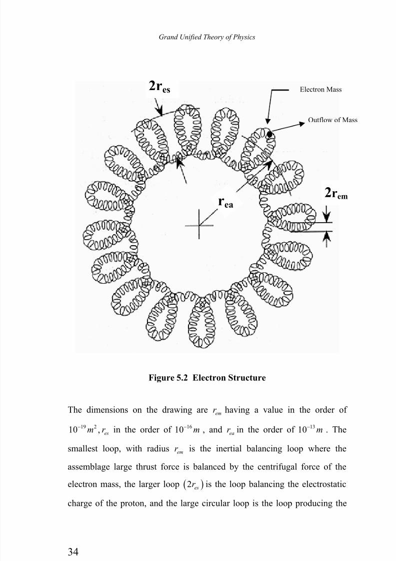
Our best model of a structure satisfying the above requirements for
the electron is presented now. 1 Figure 5.2 shows the electron structure
which is actually just the path taken by extremely small mass (having a
cross section in the order of 46 210 )m− 2, making the electron.
1 This model was first published on page 156 of Brown [11] and is shown
on the front cover of this reference.
2 The cross sectional area of the electron (core) is estimated by equating thevolume of the electron divided by the volume of the basic particle times the
particle mass to the electron mass, which is ( ) ( )3 3
4 3 4 3v b b e
r r m mπ π =⎡ ⎤⎣ ⎦ .
The area thus is ( )2 46 22 310 .
e v e b A r m m mπ
−
= This is in fair agreement with the
collision cross sectional area given by (5.15) and the core size given on page 7.
7/30/2019 The Grand Unified-mobilecrackers
http://slidepdf.com/reader/full/the-grand-unified-mobilecrackers 40/143
Grand Unified Theory of Physics
34
Figure 5.2 Electron Structure
The dimensions on the drawing are emr having a value in the order of
19 210 , esm r − in the order of 1610 m− , and
ear in the order of 1310 m− . The
smallest loop, with radius emr is the inertial balancing loop where the
assemblage large thrust force is balanced by the centrifugal force of the
electron mass, the larger loop ( )2 esr is the loop balancing the electrostatic
charge of the proton, and the large circular loop is the loop producing the
Electron Mass
Outflow of Mass
2res
2rem rea
7/30/2019 The Grand Unified-mobilecrackers
http://slidepdf.com/reader/full/the-grand-unified-mobilecrackers 41/143
Neutrino, Proton, Electron, and Neutron Structures
35
angular momentum of the electron (i.e., the spin of magnitude 2) . We
present those analyses of the loops which we have been able to develop.
Estimates have been made that the flows involved producing the
protons require less mass than the background mass so that upon formation
the proton envelope expels a mass equal to the electron mass. This expelled
excess mass is formed as one of these organized assemblages and takes a
circular path which makes it into matter (just as the translating assemblage
above produced a proton). This orbiting assemblage could be thought of as
the electron – but there are two other structural components involved togive the electron its properties.
The electron orbital (or “mass”) radius emr is controlled by
balancing the assemblage thrust (having the same value as the proton
assemblage thrust) with the centrifugal force produced by the electron mass
em . Thus
16 20
1.051545 10 1836.152668 5.7268951 10em p e pr r m m m− −
= = × = × (5.7)
Simultaneous with the formation of the small orbital inertial balancing
structure a structure must be formed to balance the positive electrostatic
field of the proton. The electrostatic field component is produced by a loop
of the inertia balancing paths. This field component must travel at the speed
of light and this disturbance is produced by the electron making all the
inertial loops. The average velocity of the electron as it advances around theelectrostatic loop is much less than the speed of light. Thus, esr is
considerably less than the proton radius, pr .
The strength of the field produced by the electron at the radius pr
is the same as that produced by the proton since both fields are caused by an
orbiting assemblage whose mass flow rate from input at velocity v m and
flow output rate at velocity vr are the same for both assemblages.
Since the velocity of propagation of the electrostatic loop around
the final circle, the angular momentum circle, is slower than the speed of
7/30/2019 The Grand Unified-mobilecrackers
http://slidepdf.com/reader/full/the-grand-unified-mobilecrackers 42/143
Grand Unified Theory of Physics
36
light. This slower speed would necessitate that the angular momentum
radius be greater than the radius required if the electron were moving at the
speed of light. This results since the angular momentum is produced by theelectron mass traveling in its nominal circular path of radius ea
r .
Some additional insight into the electron mechanism can be
obtained from the muon. The muon has a mass over 400 times the electron,
has the same charge, has angular momentum of 2 (spin 1/2) and has a
lifetime of 610− seconds. Based on the electron model the muon would have
3 structural paths: the inertial loops with radius 400 times the electron
inertial radius, the electrostatic loops (same as the electron’s), and an
angular momentum circle with a radius of 13 1510 400 10 .m− −
The
unknowns of the muon, the number of inertial and electrostatic loops and
the mass, possibly could be determined from the time-phased action of the
muon mass outflow (at the rms velocity) and the inflow (at the mean
velocity). The lifetime determination would also have to be determined
from these time-phased impulses. In summary, using the basic mechanism
of the weak nuclear force, as exemplified by the analysis of the neutron
decay, it may be possible to completely determine the masses and structures
of the electron and muon.
This model of the electron consisting of a small point mass
traversing the inertial loop, these loops traversing the electrostatic loops,and these loops traversing the angular momentum circle has implication for
the structure of the neutron.
The neutron, according to the theory here, results when pressure is
applied to the hydrogen atom (i.e., photon “mass” is added to accelerate the
orbiting electron) so that the angular momentum path is collapsed. The
remaining paths then of the electron, the inertial loops and the single
electrostatic loop, as an entity would speed up and orbit the proton at close
range. The electrostatic force would hold the (modified) electron to the
proton. The velocity of the electron is determined by its mass increase
7/30/2019 The Grand Unified-mobilecrackers
http://slidepdf.com/reader/full/the-grand-unified-mobilecrackers 43/143
Neutrino, Proton, Electron, and Neutron Structures
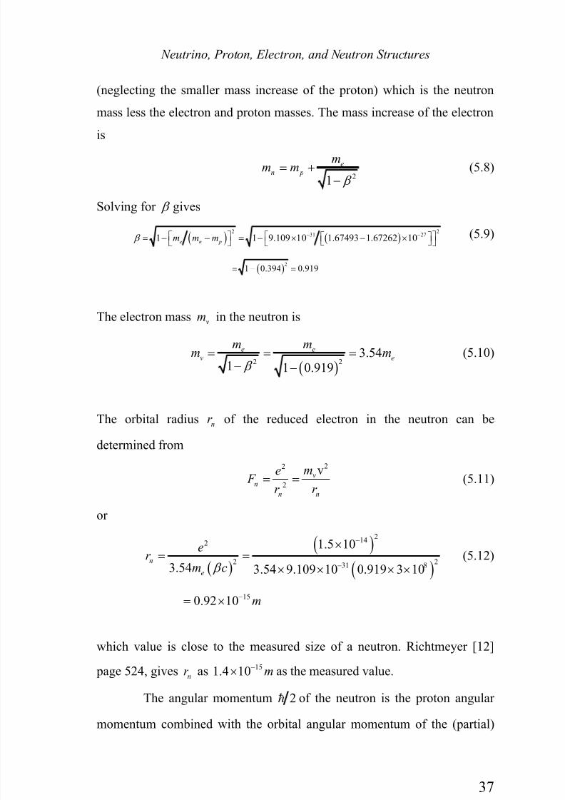
37
(neglecting the smaller mass increase of the proton) which is the neutron
mass less the electron and proton masses. The mass increase of the electron
is
21
e
n p
mm m
β = +
−(5.8)
Solving for β gives
( ) ( )22
31 271 1 9.109 10 1.67493 1.67262 10e n pm m m β − −⎡ ⎤⎡ ⎤ ⎡ ⎤= − − = − × − ×⎣ ⎦⎣ ⎦ ⎣ ⎦(5.9)
( )2
1 0.394 0.919= − =
The electron mass vm in the neutron is
( )2 2
3.541 1 0.919
e e
v e
m mm m
β = = =
− −(5.10)
The orbital radius nr of the reduced electron in the neutron can be
determined from
22
2
vv
n
nn
me F
r r = = (5.11)
or
( )
( )
( )
2142
2 231 8
1.5 10
3.54 3.54 9.109 10 0.919 3 10n
e
e
r m c β
−
−
×
= = × × × × (5.12)
150.92 10 m−= ×
which value is close to the measured size of a neutron. Richtmeyer [12]
page 524, givesn
r as 151.4 10 m−× as the measured value.
The angular momentum 2 of the neutron is the proton angular
momentum combined with the orbital angular momentum of the (partial)
7/30/2019 The Grand Unified-mobilecrackers
http://slidepdf.com/reader/full/the-grand-unified-mobilecrackers 44/143
Grand Unified Theory of Physics
38
electron (which is small) and the spinning angular momentum of the
(reduced) electron (which is small).
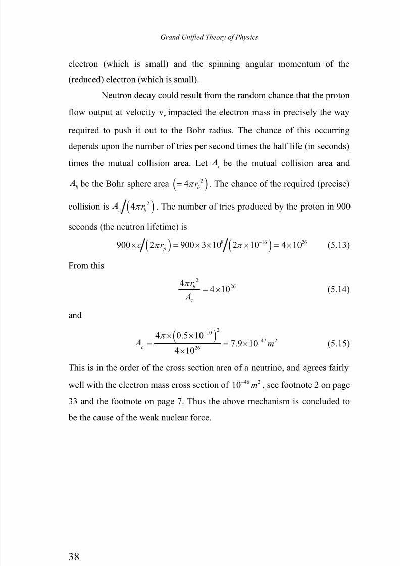
Neutron decay could result from the random chance that the protonflow output at velocity vr impacted the electron mass in precisely the way
required to push it out to the Bohr radius. The chance of this occurring
depends upon the number of tries per second times the half life (in seconds)
times the mutual collision area. Let c be the mutual collision area and
b be the Bohr sphere area ( )24b
r π = . The chance of the required (precise)
collision is ( )24c br π . The number of tries produced by the proton in 900
seconds (the neutron lifetime) is
( ) ( )8 16 26900 2 900 3 10 2 10 4 10 pc r π π −× = × × × = × (5.13)
From this
2264
4 10b
c
r
A
π = × (5.14)
and
( )2
10
47 2
26
4 0.5 107.9 10
4 10c
mπ
−
−× ×
= = ××
(5.15)
This is in the order of the cross section area of a neutrino, and agrees fairly
well with the electron mass cross section of 46 210 m− , see footnote 2 on page
33 and the footnote on page 7. Thus the above mechanism is concluded to
be the cause of the weak nuclear force.
7/30/2019 The Grand Unified-mobilecrackers
http://slidepdf.com/reader/full/the-grand-unified-mobilecrackers 45/143
Gravitation and the Non-Expanding Universe
39
6. Gravitation and the Non-Expanding Universe
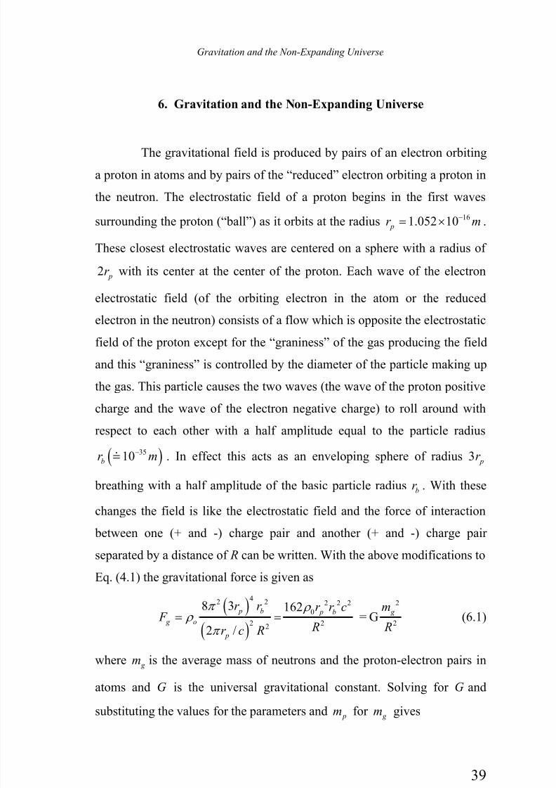
The gravitational field is produced by pairs of an electron orbiting
a proton in atoms and by pairs of the “reduced” electron orbiting a proton in
the neutron. The electrostatic field of a proton begins in the first waves
surrounding the proton (“ball”) as it orbits at the radius 161.052 10 pr m−= × .
These closest electrostatic waves are centered on a sphere with a radius of
2 pr with its center at the center of the proton. Each wave of the electron
electrostatic field (of the orbiting electron in the atom or the reduced
electron in the neutron) consists of a flow which is opposite the electrostatic
field of the proton except for the “graniness” of the gas producing the field
and this “graniness” is controlled by the diameter of the particle making up
the gas. This particle causes the two waves (the wave of the proton positive
charge and the wave of the electron negative charge) to roll around withrespect to each other with a half amplitude equal to the particle radius
( )3510b
r m− . In effect this acts as an enveloping sphere of radius 3
pr
breathing with a half amplitude of the basic particle radiusb
r . With these
changes the field is like the electrostatic field and the force of interaction
between one (+ and -) charge pair and another (+ and -) charge pair
separated by a distance of R can be written. With the above modifications to
Eq. (4.1) the gravitational force is given as
( )
( )
42 2 2 2 2 2
0
2 2 22
8 3 162= G
2 /
p b p b g
g o
p
r r r r c m F
R Rr c R
π ρ ρ
π = = (6.1)
where g m is the average mass of neutrons and the proton-electron pairs in
atoms and G is the universal gravitational constant. Solving for G and
substituting the values for the parameters and pm for g m gives

7/30/2019 The Grand Unified-mobilecrackers
http://slidepdf.com/reader/full/the-grand-unified-mobilecrackers 46/143
Grand Unified Theory of Physics
40
2 2 2 2
0162 / p b g G r r c m ρ = (6.2)
( )( ) ( ) ( ) ( )2 2 2 219 16 35 8 27162 1.0495 10 1.0516 10 1.0516 10 2.9979 10 / 1.6726 10− − −= × × × × ×
11 3 26.672 10 /m kg s−= × −
Which agrees closely with the measured value
11 3 26.673 (10) 10 /measG m kg s−= × − (6.3)
as expected since this value of G was used to determine the basic constants.
The “graniness” of the electrostatic field is also believed to be the
cause of photon decay. 1 As the photon goes through each cycle of its
translational path it apparently loses exactly one basic ether particle by a
mechanism which has not yet been identified. Assuming that this is the case
then photon dissipation would produce the same observable as an
expanding universe. The following analysis shows how this occurs.
According to the expanding universe theory the velocity "v" of
each distant star measured relative to the earth is directed from the earth to
the star and its magnitude is
v r = (6.4)
where H is the Hubble constant ( )181.80 10 /−= × , and “r” is the distance
form the earth to the star. The velocity is related to (the observed) wave
length obsλ by
v obs o
o
Hr cλ λ
λ
−= = (6.5)
where oλ is the emitted wave length. The analysis giving this equation is
limited to obsλ being less than 2 oλ , since a value greater than that would
1 This analysis grew out of a dimensional analysis interrelating microscopic,macroscopic, and cosmological parameters initiated by Dr. Robert M.Wood.

7/30/2019 The Grand Unified-mobilecrackers
http://slidepdf.com/reader/full/the-grand-unified-mobilecrackers 47/143
Gravitation and the Non-Expanding Universe
41
correspond to a star receding at a velocity greater than the speed of light. In
that case no waves would reach the earth, according to the Hubble theory.
Let us now examine the consequences resulting from the indicatedloss of one ether particle of mass b
m from a photon for each wave length of
its travel. The amount of “mass” loss per meter of the travel is
bmm
r λ
∆= −
∆(6.6)
where the negative sign indicates the reduction in mass and λ is the photon
wavelength at the time the particle is removed. Initially bm is very small
(30 orders of magnitude less than m) so that we can set /m r ∆ ∆ equal to
/dm dr . Now since 2/ E hc mcλ = = we have
b bm m mcdm
dr hλ = − = − (6.7)
Integrating gives
0 0lnm r b b
mo
m c m cdm mdr r m h m h
= − = = −∫ ∫ (6.8)
Solving for r gives
lnb o
h mr
m c m= − (6.9)
Letting om be the “mass” of the highest energy photon emitted from a
hydrogen atom we have
( )2 2 16
0 2 1 1 2 1 4 1 2.243 10o em c E E E c m J α −= = − = − = − × (6.10)
Thus
( )216 8 332.243 10 3 10 2.492 10o
m kg − −= × × = × (6.11)
Using 661.691 10b
m kg −= × gives
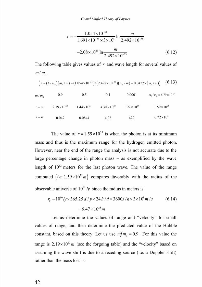
7/30/2019 The Grand Unified-mobilecrackers
http://slidepdf.com/reader/full/the-grand-unified-mobilecrackers 48/143
Grand Unified Theory of Physics
42
34
66 8 33
1.054 10ln
1.691 10 3 10 2.492 10
mr
−
− −
×= −
× × × ×
2333
2.08 10 ln2.492 10
m−= − ×
×(6.12)
The following table gives values of r and wave length for several values of
/ om m .
( ) ( ) ( ) ( )( ) ( )( )34 33/ / 1.054 10 / 2.492 10 / 0.0422 /o o o o
h m m m m m m mλ − −= = × × = × (6.13)
0/m m 0.9 0.5 0.1 0.0001 34
0/ 6.79 10
bm m −= ×
r m− 222.19 10× 231.44 10× 234.78 10× 241.92 10× 251.59 10×
mλ − 0.047 0.0844 4.22 422316.22 10×
The value of 251.59 10r = × is when the photon is at its minimum
mass and thus is the maximum range for the hydrogen emitted photon.
However, near the end of the range the analysis is not accurate due to the
large percentage change in photon mass – as exemplified by the wave
length of 3210 meters for the last photon wave. The value of the range
computed ( )25. . 1.59 10i e m× compares favorably with the radius of the
observable universe of 10
10 ly since the radius in meters is
10 8
10 365.25 / 24 / 3600 / 3 10 /ur ly d y h d s h m s= × × × × ×
(6.14)259.47 10 m= ×
Let us determine the values of range and “velocity” for small
values of range, and then determine the predicted value of the Hubble
constant, based on this theory. Let us use 0 0.9m m = . For this value the
range is 222.19 10 m× (see the forgoing table) and the “velocity” based on
assuming the wave shift is due to a receding source (i.e. a Doppler shift)
rather than the mass loss is
7/30/2019 The Grand Unified-mobilecrackers
http://slidepdf.com/reader/full/the-grand-unified-mobilecrackers 49/143
Gravitation and the Non-Expanding Universe
43
0 0
0
0
1v 1 0.111
0.9
obs obs
h h
m c m cc c c c
h
m c
λ λ
λ
−− ⎛ ⎞
= = = − =⎜ ⎟⎝ ⎠
(6.15)
Thus
815 1
22
v 0.111 3 101.52 10
2.19 10 H s
r
− −× ×= = = ×
×(6.16)
This is a thousand times larger than the measured value based on the
Doppler shift theory, ( )18 11.80 10 Doppler s− −= × .
In this kinetic particle theory of the photon the wave length shift
can be tens of orders of magnitude larger than the emitted wave length and
the wave length shift equation for the expanding universe assumption is
valid only for a shift of twice the emitted wave length (i.e., for a star at a
distance having a velocity of the speed of light). Nonetheless the predictions
of the radius of the observable universe for both theories are in fair
agreement.
7/30/2019 The Grand Unified-mobilecrackers
http://slidepdf.com/reader/full/the-grand-unified-mobilecrackers 50/143
Grand Unified Theory of Physics
44
7. Quantum Mechanics
The fundamental nature of this kinetic particle theory of physics
clearly provides the foundation of quantum mechanics. The mechanism of
the neutrino produces a single value of angular momentum for the neutrino
and provides the mechanism for making all fundamental processes move at
the speed of light. This latter mechanism, of course, is the fundamental
factor in relativity observables. The former mechanism, quantization of
angular momentum, is fundamental to all quantum effects.
The neutrino angular momentum is produced by mass rotating
about an axis. However, it is not the same as matter rotating about an axis
since it is, in effect, a "gaseous" rotating phenomenon. Also, independent
of how much mass is in the neutrino core, all neutrinos have the same
angular momentum (and particle in-flow rate).
As the neutrino whose mass is that value of mass in a proton getsinto circular orbit, it clearly will "stir" the background to produce waves.
The primary component of the wave pattern produced is the electrostatic
field. This is a field that is almost spherically symmetric. It begins
approximately at the proton radius ( )1610 m−≈ and extends until it fades
into the background ether.
Basically, the proton field is a spherical wave in a gaseous ether
which has an electrostatic potential. The mass of the proton is all
concentrated in a very small region of the proton. It is not possible to
measure (or determine) its position within the accuracy of the diameter of
the basic ether particles—at least with the techniques available from the
mainstream theory of physical science.
What we would like to do here is to show the basis for the "waveequation" representing the hydrogen atom. We will concentrate on
understanding the Schroedinger equation for the hydrogen atom without
considering the effect of electron spin or relativistic effects.
7/30/2019 The Grand Unified-mobilecrackers
http://slidepdf.com/reader/full/the-grand-unified-mobilecrackers 51/143
Quantum Mechanics
45
First, we derive the deBroglie wave equation for a moving electron.
We then derive the Schroedinger equation for a hydrogen atom.
Louis deBroglie apparently reasoned that since Albert Einstein andMax Planck had shown that light with its wave behavior had particle
behavior, matter, likewise, with its particle properties should have wave
properties. Basically he postulated that matter should translate in an
undulatory manner with a wave length given by
v
h
mλ = (7.1)
where "m" is the mass of the particle, "v" is its velocity, and h is Planck's
constant ( )2h π = .1 In this present theory we derive, instead of postulate
Eq.(7.1).
Recall that the structure of an electron consists of a very small
neutrino orbiting in a very small path (10-20 m in diameter). This path is a
perturbation to the larger path (103 times the diameter of the neutrino orbital
path) which produces the electrostatic field. This larger path is a
perturbation to the even larger path (103 times the diameter of the
electrostatic field path) which is the path producing the electron angular
momentum. It turns out that the wave property of an electron, as
represented by the deBroglie relation and as used in the Schroedinger
equation, is a very simple part of the complex structure of the electron field.
In order to understand the origin of the deBroglie relation, we need
to recall how an electron has its velocity changed. Imagine an electron at
rest (knowing full well that an electron can never be at rest), which means
that the center of the angular momentum field is at rest. Now, impact the
electron by a low energy photon. The electron captures the photon and the
1Apparently, deBroglie thought of the electron being embedded in a "pilot"
wave, which is similar to the theory presented here.
7/30/2019 The Grand Unified-mobilecrackers
http://slidepdf.com/reader/full/the-grand-unified-mobilecrackers 52/143
Grand Unified Theory of Physics
46
two entities become one entity which is translating at velocity v. 1 The
angular momentum of the photon before capture was . The angular
momentum increase resulting to the electron, i.e., for the two combinedentities is vmr = , where r is the half-amplitude of the electron wave.
Since the photon always moves at velocity c, it must be captured at a great
distance from the angular momentum center. Linear momentum
conservation also shows that the radius must be very large since the
captured photon still continues moving at velocity c and the electron photon
assembly moves only at velocity v, where v << c. The frequency of the
wave, then, is v 2c r cπ λ = = . Using 2r λ π = gives
( )2 vh m λ π = (7.2)
or
2 vh mπ λ = = (7.3)
and
( )vh m h pλ = = (7.4)
where p is the matter particle momentum. This, of course, is the deBroglie
relation.
The extension of this equation to the relativistic case, of course,
requires accounting for the mass actually added to the electron.
Before going on to the Schroedinger equation, we should mention
the so-called double slit experiment. When electrons pass through a screen
with a single slit, they produce a Gaussian type dispersal pattern on a
"screen." This pattern results since the relative position of the wave phase
and the slit vary from one electron to the next. When the electron goes
through the slit, all of its field is squeezed down and goes through that
single hole. When a second slit is opened and if the electrons still pass
through the initial slit, there is a diffraction pattern on the screen. The
1 The portion of the electron field which captures the photon is theelectrostatic field component, and not the larger radius angular momentumfield nor the smaller force balance field.
7/30/2019 The Grand Unified-mobilecrackers
http://slidepdf.com/reader/full/the-grand-unified-mobilecrackers 53/143
Quantum Mechanics
47
diffraction pattern results because of the wave phase and slit position
varying and because of part of the electron field passing through the second
slit.The key to this phenomenon is that the electron itself is a very
small item, and the field is a very extensive item. It is anticipated that the
pattern which results on the screen for electrons actually passing through
one slit would differ from, but be symmetric with the pattern for electrons
passing through the other slit. Incidentally, photons from lasers, for
example, should be directable to pass through a pre-selected slit and thus
show the different, but symmetric, patterns for the two slits. The electron is
a very small particle, but it has a large energy since its energy is
( )30 8 1310 3 10 10e
m c22 − −= × = joules. (7.5)
This energy of the moving mass also is the same as the energy of motion of
its field, i.e., the energy stirred up in the background. These dynamic
effects produced by the motion in the background are what we observe.When we observe its effects, we say we observe the electron. In this sense
we can talk about the electron at a given time being distributed over a
region of space. The energy per unit volume varies with time and location
since the energy is a wave. This wave has the general equation
( ) ( ),i kx t
o x t e
ω ψ ψ
−= (7.6)
which is the wave generated by an electron translating along an advancing,
but sinusoidal, path. Even though we have used the familiar wave function
symbol ψ , do not assume it is necessarily the function ψ used by quantum
electrodynamicists. We hope here to define this ψ strictly from a classical
Newtonian basis. We will return to this shortly.
The conservation of energy for the electron is
( )2 p m P E 2 + = (7.7)
7/30/2019 The Grand Unified-mobilecrackers
http://slidepdf.com/reader/full/the-grand-unified-mobilecrackers 54/143
Grand Unified Theory of Physics
48
where E is the electron's total energy, " P " is the electron's potential energy,
and " p" is its momentum (p = mv). Thus, ( )2 v 2 p m m2 2= is the
electron's kinetic energy.
If we want to predict anything about the detailed structure of the
electron, i.e., of the electron field produced by the elusive neutrinos, then
we can multiply each of the above three terms by a distribution function of
space and time which, when evaluated, will give the characteristics of this
field for any location and time. We thus have
( )2 p m P E ψ ψ ψ 2 + = (7.8)
Using the deBroglie relation for all matter particles, we have
h pλ = (7.9)
or
( )( )2 2 p h h x k λ π π = = = (7.10)
where k is the space variation frequency in the wave equation. Using the
Einstein relation (which we have derived classically from this theory), we
have
( )( )2 2 E h hλ π πλ ω = = = (7.11)
The energy equation can be written as
( )2k m P ψ ψ ωψ 2 2⎡ ⎤ + =⎣ ⎦ (7.12)
Noting that
x ik t iψ ψ ψ ωψ ∂ ∂ = ∂ ∂ = (7.13)
we can write this energy equation as
( ) ( )2h m x P i t ψ ψ ψ 2 2 2− ∂ ∂ = = ∂ ∂ (7.14)
This, of course, is the Schroedinger time dependent wave equation for one
dimension.
7/30/2019 The Grand Unified-mobilecrackers
http://slidepdf.com/reader/full/the-grand-unified-mobilecrackers 55/143
Quantum Mechanics
49
The function ψ can be a velocity (as well as a square root of
energy) function. The functionψ can be defined in such a way that ψ 2
gives the energy density function. The function ψ is called the probability
amplitude. The energy E contained in a volume ∆ V at a given point is
E ψ ψ * ∆ V. The electron energy is
( ) ( ) E V dV E V dV mcψψ ψψ 2= ∗ =∫ ∫ . (7.15)
Further, note that
( )1 1.0V dV ψψ ∗ =∫ , (7.16)
which is the usual definition of a normalized distribution function.
We note here that ψ itself is similar to a planar velocity since
ψ ψ * is like the square of two velocity components1 so that ψ ψ * is
similar to an energy. Thus ψ is a space and time distribution function of
the electron field energy. The occurrence of an "i" on the right side of the
Schroedinger equation indicates a 90-degree shift of phase for the velocity.
The occurrence of the second partial of ψ with respect to distance and the
first partial derivative with respect to time, as well as the phase shift, are the
direct result of a classical wave function satisfying the energy equation.
In the early years of development of quantum mechanics, there
were two interpretations of the wave function ψ . One was that the electron
somehow was spread out over space and ψ was its mass distribution
function which, of course, is the interpretation here. It is emphasized that
this is a classical Newtonian interpretation when the electron field is being
considered instead of the electron itself. However, physicists in the 1920s
were not considering the electron as being a flow of classic kinetic particles.
1 Recall that for two complex number A and B, where A = r + is and B = r –
is, that AB* is r s2 2+
7/30/2019 The Grand Unified-mobilecrackers
http://slidepdf.com/reader/full/the-grand-unified-mobilecrackers 56/143
Grand Unified Theory of Physics
50
The second interpretation of ψ ψ *, due to Max Born in the 1920s,
is that it is the probability density function such that ψ ψ * ∆ V/V gives the
probability of finding the electron in the particular differential volume ∆ V1
(more precisely, in the volume 1 x to 1 1, x y+ ∆ to 1 1, y y z + ∆ to 1 z z + ∆
where ψ ψ * is evaluated at x1 y1 z 1). It appears that quantum physicists
took a wrong turn there by accepting the Born interpretation. However,
without the field description developed in this present theory, the first
interpretation seemed very bizarre.
Let us continue with our interpretation of ψ . The space and time
variables are easy to separate. We write
( ) ( ) ( ) ( ),i kx t iky i t t Ae Ae e x f t
ω ω ψ ϕ
− −= = ⋅ = ⋅ (7.17)
Substituting into the one dimensional wave equation gives
( ) ( ) ( ) ( ) ( )2h m x f t P x x f t ψ ψ 2 2 2− ∂ ∂ ⋅ + ⋅ (7.18)
( )i x f t ψ = ⋅ ∂ ∂
Dividing each term by ( ) ( ) x f t ψ ⋅
gives
( ) ( ) ( )( ) ( )2 1h m x x P xψ ψ 2 2 2− ∂ ∂ + (7.19)
( ) ( )i f t f t = ∂ ∂
The left side is a function of x only, and thus equals a constant, or
zero. The right side is equal to the negative of the constant. We let the
constant be unity for the previous interpretation of ψ . However, without
loss of generality and to be in line with current practice, we redefine ψ so
that dV ψψ ∗∫ is equal to the total energy of the particle E . Thus we will
take the separation constant to be E . Now, the two equations are total
differential equations, and are
7/30/2019 The Grand Unified-mobilecrackers
http://slidepdf.com/reader/full/the-grand-unified-mobilecrackers 57/143
Quantum Mechanics
51
( ) ( )df dt iE f t = − (7.20)
for the right side and for the left side
( ) ( ) ( ) ( )2m d dx P x x E xψ ψ ψ 2 2 2− + = i (7.21)
The solution for the first equation is
( ) i t f t Ce ω −= (7.22)
For solving the second equation, we write it as
( )( )2m d dx P E ψ ψ 2 2 2− + = (7.23)
or
Q E ψ ψ = (7.24)
where we define the operator
( )( )2Q m d dx P 2 2 2= − + (7.25)
We define ψ then over the complete region of the electron and
then V E
ψψ ∗
gives the distribution function of the electron field energy asa function of the space coordinates (x, y, z) and time. The integral over the
volume is the total energy E . This energy divided by c2 then is the electron
mass.
The undulatory path of the electron gives the quantitization of
orbits for the atoms as postulated by Bohr and as shown by deBroglie with
his postulated waves.
Here we have shown the classical basis of the electron wave.
Knowing that, we have a wave distribution of the electron and we have used
a wave energy distribution function with the electron conservation of
energy equation and have shown that gives the Schroedinger equation. We
are now in a position, based strictly on a classical theory, to write the
Schroedinger equation for the hydrogen atom.
The three-dimensional time-dependent Schroedinger equation is
( ) ( ) ( ) ( ), , , , , , , , , , ,2
y z t P x y z x y x t i x y z t t m
ψ ψ ψ 2− ∇ + = ∂ ∂
(7.26)
7/30/2019 The Grand Unified-mobilecrackers
http://slidepdf.com/reader/full/the-grand-unified-mobilecrackers 58/143
Grand Unified Theory of Physics
52
where
x y z
2 2 22
2 2 2
∂ ∂ ∂∇ = + +
∂ ∂ ∂(7.27)
We write
( ) ( ), , , , , i t x y z t x y z e ω ψ ϕ = (7.28)
and substituting into the right side of the general Schroedinger equation
gives
( ) ( ) ( ) ( ) ( )2 , , , , , , , , , ,
2
i t x y z t x y z x y z t i i x y z e
m
ω ψ ρ ψ ω ϕ −− ∇ + = −
(7.29)
( ) ( ), , , ,i t i t x y z e E x y z eω ω ωϕ ϕ − −= =
where E ω = . Thus we have
( ) ( ) ( ) ( ), , , , , , , ,2
i t i t i t y z e P x y z x y z e E x y z em
ω ω ω ϕ ϕ ϕ 2 − − −− ∇ + =
(7.30)
Canceling out the i t e ω − gives the time-independent Schroedinger equation
( ) ( ) ( ) ( ), , , , , , , ,2
x y z P x y z x y z E x y z m
ϕ ϕ ϕ 2− ∇ + =
(7.31)

7/30/2019 The Grand Unified-mobilecrackers
http://slidepdf.com/reader/full/the-grand-unified-mobilecrackers 59/143
Quantum Electrodynamics
53
8. Quantum Electrodynamics
a. The Electron Two Slit Experiment
The kinetic particle theory of physics clearly provides the structure
underlying all of quantum theory. Thus, any observation explained by
quantum electrodynamics must be explained by the kinetic particle theory
of physics. One of the most interesting (and, mysterious) phenomenon is the
“double-slit” experiment. We show here how the kinetic particle theory
explains the “double-slit” experiment for electrons.
Figure 8.1 shows an electron emitter, a “target” with two slits, and
a detector screen. Figure 8.2 shoes the two slits and electron hit densities for
the three cases of right slit open, left slit open, and both slits open.
Electron GunElectron
TargetScreen
Figure 8.1. Double-Slit Experiment
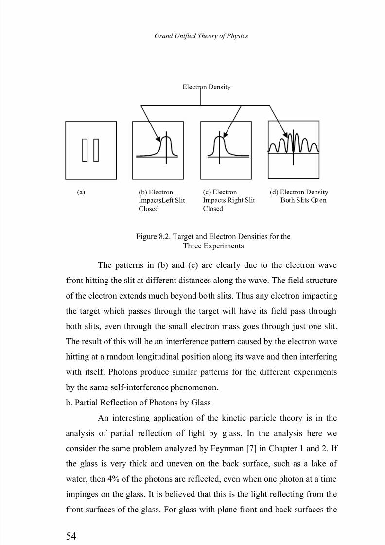
7/30/2019 The Grand Unified-mobilecrackers
http://slidepdf.com/reader/full/the-grand-unified-mobilecrackers 60/143
Grand Unified Theory of Physics
54
The patterns in (b) and (c) are clearly due to the electron wave
front hitting the slit at different distances along the wave. The field structure
of the electron extends much beyond both slits. Thus any electron impacting
the target which passes through the target will have its field pass through
both slits, even through the small electron mass goes through just one slit.
The result of this will be an interference pattern caused by the electron wave
hitting at a random longitudinal position along its wave and then interfering
with itself. Photons produce similar patterns for the different experiments
by the same self-interference phenomenon.
b. Partial Reflection of Photons by Glass
An interesting application of the kinetic particle theory is in the
analysis of partial reflection of light by glass. In the analysis here we
consider the same problem analyzed by Feynman [7] in Chapter 1 and 2. If
the glass is very thick and uneven on the back surface, such as a lake of
water, then 4% of the photons are reflected, even when one photon at a time
impinges on the glass. It is believed that this is the light reflecting from the
front surfaces of the glass. For glass with plane front and back surfaces the
Electron Density
(a) (b) ElectronImpactsLeft SlitClosed
(c) ElectronImpacts Right SlitClosed
(d) Electron DensityBoth Slits O en
Figure 8.2. Target and Electron Densities for theThree Experiments
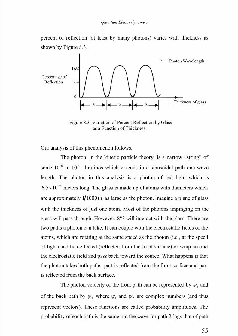
7/30/2019 The Grand Unified-mobilecrackers
http://slidepdf.com/reader/full/the-grand-unified-mobilecrackers 61/143
Quantum Electrodynamics
55
percent of reflection (at least by many photons) varies with thickness as
shown by Figure 8.3.
Our analysis of this phenomenon follows.
The photon, in the kinetic particle theory, is a narrow “string” of
some 2010 to 3010 brutinos which extends in a sinusoidal path one wave
length. The photon in this analysis is a photon of red light which is
76.5 10−× meters long. The glass is made up of atoms with diameters which
are approximately 1 1000th as large as the photon. Imagine a plane of glass
with the thickness of just one atom. Most of the photons impinging on the
glass will pass through. However, 8% will interact with the glass. There are
two paths a photon can take. It can couple with the electrostatic fields of the
atoms, which are rotating at the same speed as the photon (i.e., at the speed
of light) and be deflected (reflected from the front surface) or wrap around
the electrostatic field and pass back toward the source. What happens is that
the photon takes both paths, part is reflected from the front surface and part
is reflected from the back surface.
The photon velocity of the front path can be represented by 1ψ and
of the back path by 2ψ where 1ψ and 2ψ are complex numbers (and thus
represent vectors). These functions are called probability amplitudes. The
probability of each path is the same but the wave for path 2 lags that of path
λ λ λ
0
8%
16%
Percentage of Reflection
λ — Photon Wavelength
Thickness of glass
Figure 8.3. Variation of Percent Reflection by Glass
as a Function of Thickness

7/30/2019 The Grand Unified-mobilecrackers
http://slidepdf.com/reader/full/the-grand-unified-mobilecrackers 62/143
Grand Unified Theory of Physics
56
1 by the slight time required to go around the atom. Thus, the direction of
the two vectors are slightly different and the “senses” are almost opposite,
see Figure 8.4. What happens is that the photon splits and actually takes both paths.
For path 2 after the photon portion turns 180º (which the photon travels the
distance ( )2 1000π λ inside the glass) and its flow velocity is opposite that
of the incoming part. “Self Interference” thus cancel the photon, most of the
time. The photon energy is proportional to the square of the velocity. Thus
2
1 2ψ ψ + is the probability of the photon being reflected by the front and
back surface. Clearly2
1 2ψ ψ + is very small compared to2
1ψ and2
2ψ
since the glass thickness is so small compared to the photon “length”.
As the glass becomes thicker the angle α , in Figure 8.4, becomes
larger and larger reaching π radians when the glass thickness is 2λ . At
that thickness the percentage of reflection is 16%, 12% from the back
surface and 4% from the front surface. At one atom thickness we say the
front surface reflects 4% and the back surface reflects 4% of the photons,
but the two are almost exactly out of phase so that practically no photons
are reflected.
Figure 8.4 shows the physical significance of the arrows used in
quantum electrodynamics. The arrows are used to determine the phasings of
the portions of a photon.
c. Diffraction of Light
1ψ
2ψ 1ψ + 2ψ
α
Figure 8.4 Velocities of Reflecting Photon For the Two Paths
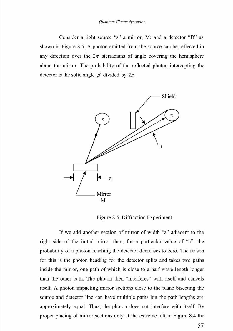
7/30/2019 The Grand Unified-mobilecrackers
http://slidepdf.com/reader/full/the-grand-unified-mobilecrackers 63/143
Quantum Electrodynamics
57
Consider a light source “s” a mirror, M; and a detector “D” as
shown in Figure 8.5. A photon emitted from the source can be reflected in
any direction over the 2π sterradians of angle covering the hemisphereabout the mirror. The probability of the reflected photon intercepting the
detector is the solid angle β divided by 2π .
If we add another section of mirror of width “a” adjacent to the
right side of the initial mirror then, for a particular value of “a”, the
probability of a photon reaching the detector decreases to zero. The reason
for this is the photon heading for the detector splits and takes two paths
inside the mirror, one path of which is close to a half wave length longer
than the other path. The photon then “interferes” with itself and cancels
itself. A photon impacting mirror sections close to the plane bisecting thesource and detector line can have multiple paths but the path lengths are
approximately equal. Thus, the photon does not interfere with itself. By
proper placing of mirror sections only at the extreme left in Figure 8.4 the
SD
β
Shield
a
Mirror M
Figure 8.5 Diffraction Experiment
7/30/2019 The Grand Unified-mobilecrackers
http://slidepdf.com/reader/full/the-grand-unified-mobilecrackers 64/143
Grand Unified Theory of Physics
58
detector can “see” the source. Such placement of mirror sections produces a
diffraction grating.
7/30/2019 The Grand Unified-mobilecrackers
http://slidepdf.com/reader/full/the-grand-unified-mobilecrackers 65/143
Closure
59
9. Closure
The kinetic particle theory of physics provides the following:
1. The fine structure constant is the ratio of force due to the root
mean square velocity less the mean velocity, the difference divided
by the force due to the mean velocity of the background ether.
2. All matter at rest is made up of kinetic particles moving in a
circular path at the speed of light so that the energy of all matter is
its mass times the square of the speed of light.
3. A proton is made of a single small orbiting assemblage of
background particles.
4. Mass is added to matter to accelerate it so that the mass at velocity
is the rest mass divided by 21 β − , where β is the matter velocity
in speed of light units.
5. When mass is added to accelerate matter the mass is added
eccentrically so that the mass is still moving at the speed of light
but taking a spiral path. The spiral path takes longer to cycle than
when at rest (giving time dilation) and shortens the matter when
viewed from a frame translating with the matter.
6. The eccentric mass causes mass to undulate as it moves then this
gives matter its wave property.
7. The mass making up a proton or an electron moving in a circular
path sets up the electromagnetic field which produces electrostatic
forces.
8. The translating wave produces magnetism by the same mechanism
that the rotating mass causes electrostatic forces.
9. The electron structure consists of a single concentrated mass taking
a path in a loop which balances the inertial forces, a larger loop
which produces the electrostatic field, and a third even larger
complete circle loop that produces the electron angular momentum.

7/30/2019 The Grand Unified-mobilecrackers
http://slidepdf.com/reader/full/the-grand-unified-mobilecrackers 66/143
Grand Unified Theory of Physics
60
10. The neutron results when a sufficiently large pressure is applied to
a hydrogen atom so that the angular momentum loop of the
electron is collapsed and centrifugal force is balanced by the strongnuclear force when the collapsed electron orbits the proton.
11. The weak nuclear force is due to the strong nuclear force less the
result of the chance encounter with the output from a basic matter
particle assembly where the output mass is moving at the rms
velocity of the background ether.
12. Gravitation is caused by two orbiting balanced opposite charges
except for that prohibited by the actual basic ether particle size
making up all the contents of the universe.
13. The Hubble red shift of star light is caused by photons losing one
basic ether particle for each wave length of travel, and giving the
illusion of an expanding universe.
14. The kinetic particle flows producing the fields of particles are
modeled using the equations of quantum mechanics.
15. Kinetic particle theory explains the double-slit experiments for
electrons and photons as well as partial reflection and diffraction
grating experiment.
7/30/2019 The Grand Unified-mobilecrackers
http://slidepdf.com/reader/full/the-grand-unified-mobilecrackers 67/143
Appendix A. Determination of the Basic Constants of Physics
61
Appendix A. Determination of the Basic Constants of Physics
A universe containing only a gas of inert hard elastic spherical
particles of one size requires four, and only four, parameters to completely
define it. The four we have selected here are the mean speed of the particle
( )vm(measured relative to a frame for which there is no net flow of gas, i.e.,
a rest frame), the mass of the individual particle ( )bm , the radius of the
particle ( )br , and the mean free path for the gas ( )l . It is obvious that the
first three parameters are required, they give the properties of mass, length,
and time to the theory. However, if two universes were imagined with the
same particle mass, diameter, and speed but a different mean free path then
the two universes would be different. For example if the first universe had a
mean free path of 4 particles radii and the other a mean free path of 4,000,000 radii, they certainly would be different universes.
If the universe actually were a kinetic particle universe and if we
understood the mechanisms by which everything functioned then we should
be able to find four independent measured constants for which the four
basic constants of this theory could be determined. As it so happens we
have an approximate understanding of four different (independent)
mechanisms which provide an exact value (within measurement error) for
one constant and approximate values for the other three.
The measured constants we use are the speed of light, the value of
the basic electron charge, the mass of the proton, and the universal
gravitational constant. The mechanisms we use are the one controlling the
speed of light for the neutrino, the mechanism producing the electrostatic
charge, the mechanism producing gravity, and the mechanism of the
neutrino. The measured constants we use are c (the speed of light), e (the
charge of the electron), pm (the mass of the proton), and G (the universal
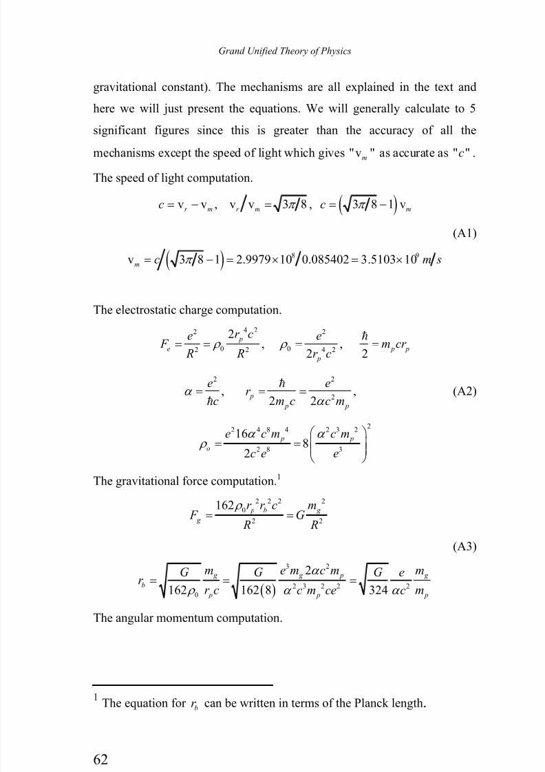
7/30/2019 The Grand Unified-mobilecrackers
http://slidepdf.com/reader/full/the-grand-unified-mobilecrackers 68/143
Grand Unified Theory of Physics
62
gravitational constant). The mechanisms are all explained in the text and
here we will just present the equations. We will generally calculate to 5
significant figures since this is greater than the accuracy of all themechanisms except the speed of light which gives "v "m as accurate as " "c .
The speed of light computation.
( )v v , v v 3 8 , 3 8 1 vr m r m mc cπ π = − = = −
(A1)
( )
8 9v 3 8 1 2.9979 10 0.085402 3.5103 10mc m sπ = − = × = ×
The electrostatic charge computation.
4 22 2
0 02 2 4 2
2, ,
22
p
e p p
p
r ce e F m cr
R R r c ρ ρ = = = =
2 2
2, ,
2 2
p
p p
e er
c m c c m
α
α
= = =
(A2)
22 4 8 4 2 3 2
2 8 3
168
2
p p
o
e c m c m
c e e
α α ρ
⎛ ⎞= = ⎜ ⎟⎜ ⎟
⎝ ⎠
The gravitational force computation.1
2 2 2 2
0
2 2
162
p b g
g
r r c m F G
R R
ρ = =
(A3)
( )
3 2
2 3 2 2 2
0
2
162 162 8 324
g g p g
b
p p p
m e m c m mG G G er
r c mc m ce c
α
ρ α α = = =
The angular momentum computation.
1 The equation for br can be written in terms of the Planck length.
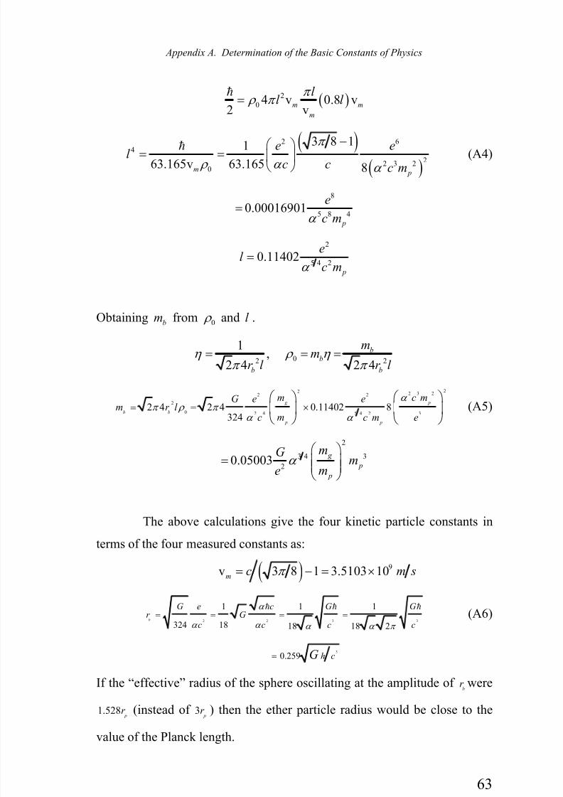
7/30/2019 The Grand Unified-mobilecrackers
http://slidepdf.com/reader/full/the-grand-unified-mobilecrackers 69/143
Appendix A. Determination of the Basic Constants of Physics
63
( )2
0 4 v 0.8 v2 v
m m
m
l l l
π ρ π =
( )( )
2 64
22 3 20
3 8 11
63.165v 63.165 8m p
e el
c c c m
π
ρ α α
−⎛ ⎞= = ⎜ ⎟⎝ ⎠
(A4)
8
5 8 40.00016901
p
e
c mα =
2
5 4 20.11402
p
el
c mα =
Obtainingb
m from 0 ρ and l .
02 2
1,
2 4 2 4
b
b
b b
mm
r l r l η ρ η
π π = = =
22 2 3 22 2
2
0 2 4 5 4 2 32 4 2 4 0.11402 8
324
g p
b b
p p
m c mG e em r l
mc c m e
α π ρ π
α α
= = ×⎛ ⎞⎛ ⎞⎜ ⎟⎜ ⎟
⎝ ⎠ ⎝ ⎠
(A5)
2
3 4 3
20.05003
g
p
p
mGm
meα
⎛ ⎞= ⎜ ⎟⎜ ⎟
⎝ ⎠
The above calculations give the four kinetic particle constants in
terms of the four measured constants as:
( ) 9v 3 8 1 3.5103 10m
c m sπ = − = ×
2 2 3 3
1 1 1
324 18 18 18 2b
G e c G Gr G
c c c c
α
α α α α π
= = = =
(A6)
3
0.259 h cG=
If the “effective” radius of the sphere oscillating at the amplitude of b
r were
1.528 pr (instead of 3
pr ) then the ether particle radius would be close to the
value of the Planck length.

7/30/2019 The Grand Unified-mobilecrackers
http://slidepdf.com/reader/full/the-grand-unified-mobilecrackers 70/143
Grand Unified Theory of Physics
64
( )
10 14
35
2 28
.6673 10 1.5189 10 11.0510 10
324 324 0.0072974 2.9979 10
g
b
p
mG er m
mcα
− −
−× ×= = = ×
×
( ) ( )
( )
32 3 411 27
3 4 3
2 214
0.05003 6.673 10 0.0072974 1.6726 100.05003
1.5189 10
g
b p
p
mGm m
meα
− −
−
× × × ×= =
×
⎛ ⎞⎜ ⎟⎝ ⎠
661.6906 10 kg −= × (A7)
( )
( ) ( ) ( )
2142
5 4 2 25 48 27
0.11402 1.5189 100.11402
.0072974 2.9979 10 1.6726 10 p
el
c mα
−
−
×= =
× ×
178.2045 10 m−= ×
The four derived constants are
9v 3.5103 10 /m
m s= ×
351.0510 10b
r m−= × (A8)
661.6906 10b
m kg −= ×
178.2045 10l m−= ×
Other parameters often needed are
0.0072974α =
( )34
16
27 8
1.0546 10 1.0516 102 2 1.6726 10 2.9979 10
p
p
r mm c
− −
−×= = = ×
× × ×
( )
( ) ( )
2142
19 3
0 4 2 4 216 8
1.5189 101.0495 10 /
2 2 1.0516 10 2.9979 10 p
ekg m
r c ρ
−
−
×= = = ×
× ×
(A9)
19
84 3066
1.0495 10 6.2079 101.6906 10
b
mm ρ η −
−×= = = ××

7/30/2019 The Grand Unified-mobilecrackers
http://slidepdf.com/reader/full/the-grand-unified-mobilecrackers 71/143
Appendix B. Further Discussion of the Neutrino Structure
65
Appendix B. Further Discussion of the Neutrino Structure
All the analysis in this paper is based on the premise that stable
inhomogeneous states can exist in a gas consisting of hard elastic particles
which interact only by repulsion when they collide. We are familiar with
hurricanes, cyclones, and tornados. These flow patterns are stable
inhomogeneous assemblages of air molecules. Comprehensive analyses
showing the mechanisms of their stability have not been developed.
However, the observed stability of tornados, etc, which are made up of gases with electromagnetic properties and which involve heat flow does not
prove that a gas of inert particles could form a stable inhomogeneous state.
These flows open the question but do not lead us to a conclusion for or
against a stable inhomogeneous state of inert particles.
We also know that all macroscopic inhomogeneous states of inert
particles which we observe always dissipate and move toward homogeneity.
In contrast, the stable inhomogeneous states we are considering in this
paper are contained within a sphere with a diameter of one mean free path
of the ether gas, which value is 1610 m− . Further, the observed particles of
this theory, i.e., the condensed regions of all the inhomogeneous
assemblages are in the order of 2310− meters. If the same inhomogeneous
phenomenon existed with air molecules as with the basic ether gas particles
then the air assemblages would exist inside a sphere with a radius equal the
mean free path of 610 m− and the solid core diameter would be smaller than
this. Such assemblages could occur without being recognized as having the
structure of the inhomogeneous assemblages of this theory. Possibly such
assemblages in the atmosphere could be the origin of hail and raindrops.
Scientists have tried for more than a century to find a stable
inhomogeneous state and have tried to prove that a stable inhomogeneous
state for kinetic particles can not exist. So far, science has failed in both
7/30/2019 The Grand Unified-mobilecrackers
http://slidepdf.com/reader/full/the-grand-unified-mobilecrackers 72/143
Grand Unified Theory of Physics
66
endeavors. Clearly in any theory of physics there must be some mechanism
for producing inhomogeneous states, since the universe is inhomogeneous.
The results of this paper argue strongly for the existence of stableinhomogeneous assemblages of the hypothesized ether gas. Verification of
the stable assemblage possibly could be obtained experimentally using gas
molecules with a very long mean free path or by a dynamic analysis.
The stable inhomogeneous states which is envisioned for this
theory consists of a particle flow configuration which is essentially
contained within a sphere with a radius in the order of one mean free path of
the background gas. The concept of this theory is to begin with a uniform
(homogeneous) gas and construct one basic type of inhomogeneous
assembly. This inhomogeneous assembly then forms hydrogen atoms which
produce a flow of particles which is the gravitational field. Hydrogen atoms
are gravitationally attracted to each other to produce large assemblages
(stars) and then other atoms. The basic assemblage of this theory thus not
only is inhomogeneous but it also provides a mechanism for producing
other inhomogeneties for further organizing the universe.
We have spent an appreciable amount of effort attempting to
develop a dynamic analysis of the hypothesized state. We consider the
analysis in three different regions:
1. A radial inflow into a spherical sink where the inflow reaches
sonic speed at a spherical surface with a diameter in the order of
the mean free path of the gas. Initially the sphere is considered to
be at rest but later we planned to determine the inflow to the sphere
when it translates at the speed of v vr m− (the rms speed less the
mean speed of the background gas).
2. An inflow from the sonic speed spherical surface using curved
stream tubes down to the solid cylindrically shaped core of the
assemblage.
7/30/2019 The Grand Unified-mobilecrackers
http://slidepdf.com/reader/full/the-grand-unified-mobilecrackers 73/143
Appendix B. Further Discussion of the Neutrino Structure
67
3. An axial inflow into the aft end of the solid cylindrical core at
velocity vm
, impacts on the sides of the cylindrical surface to
completely condense the core and to accelerate it from velocity vm
to velocity vr
, and an output from the front of the core at
velocity vr .
The basic conservation equations governing the particle flows for
the envisioned inhomogeneous assemblage are the conservation of mass,
linear momentum in three directions, angular momentum in three directions,
and energy; eight conservation equations total. In addition there are the
equations of state. One usually used is the ideal gas equation 21v
3r
p ρ = ;
where p is the pressure, ρ is the mass density, and vr
is the rms velocity,
which velocities are measured relative to the flowing gas. Another state
equation is for the solid in the region where the particles are touching each
other. The flow analysis is conventional except for handling the gas
equation of state when the gas takes a curved path.
When gas flowing in a straight path becomes perturbed into a
curved path half of the particles have thermal velocity components opposite
the velocity and half in the same direction as the flow velocity. The half
with opposite components have radial centrifugal forces that are smaller
than the half with components in the same sense as the flow velocity. As a
result there is a transient radial adjustment which accentuates the curvature
since the slower particles will move inward and the faster particles will
move outward. This transient radial adjustment further accentuates the
curvature since removal of the particles with aft thermal components
increase the flow velocity at the outer stream tubes. Similarly, adding aft
thermal component particles opposite the flow decreases the flow speed atthe inner stream tubes. When the steady state is reached and the curvature
becomes constant the equation of state may be homogeneous (i.e.,

7/30/2019 The Grand Unified-mobilecrackers
http://slidepdf.com/reader/full/the-grand-unified-mobilecrackers 74/143
Grand Unified Theory of Physics
68
21v
3r
p ρ = ) or it may be skewed as a result of the inertial field acting upon
the particles. In any case the separation of particles due to their thermalvelocities (i.e., thermal separation) as a result of curved flow may be the
mechanism causing hurricane winds to take their circular paths. Further,
tornados, “dust devils”, and turbulent vortices may also be due to this
mechanism.
The phenomenon of thermal separation because of a gas taking a
curved path is well documented in the case of vortex tubes. A vortex tube is
a hollow cylinder into which a gas is injected at the periphery perpendicular
to the cylinder longitudinal axis. The air enters and is immediately forced
into a spiral path as it rotates and advances along the cylindrical
longitudinal axis. At the exit from the cylinder (which is open at least on
one end) the gas at the periphery can be tens to a hundred degrees greater
than the inlet gas temperature and at the cylinder axis it can be tens to a
hundred degrees cooler than the inlet gas.
Let us present some more discussion of tornados and hurricanes to
provide additional insight into the mechanism of the stable state envisioned
for this theory. Consider first the question of what produces the curved
flows in hurricanes and tornados – and, further, for vortices in general.
Consider a mass of air moving in a straight path. Assume a low pressure
region occurs on one side of the moving mass or that it intercepts another
moving mass in such a way that it will produce curvature of the straight
path. In order to understand the response of air when deflected into a curved
path we need to consider the individual molecule.
Air moving in a straight path has a flow velocity and a thermal
velocity. The flow velocity is the average of the components of the
individual molecules along the direction for which the average is amaximum. The thermal velocity of a molecule is the molecule velocity less
the flow velocity. The thermal speeds at a point have the same distribution
7/30/2019 The Grand Unified-mobilecrackers
http://slidepdf.com/reader/full/the-grand-unified-mobilecrackers 75/143
Appendix B. Further Discussion of the Neutrino Structure
69
along every direction over 4π sterradians. They have the Maxwell-
Boltzmann distribution.
When the gas begins to take a curved flow path it is not generallyknown how the gas behaves. One thing is clear, however, if we divide the
molecules into two equal number categories. Half of the molecules have
thermal velocities which have components along the flow velocity with the
same sense as the flow velocity and half will have components in the
opposite sense. The response of the molecules to the “inertial field” of the
curved path will depend only upon the magnitude of the individual
molecule velocity component parallel to the flow velocity. The average
response of that half of the molecules with thermal components adding to
the flow velocity, i.e., with an average component of v v 2 f r + where v
f
is the flow velocity and vr
is the group thermal velocity, will be a radial
inward acceleration of ( )v v 2 f r
r + where r is the radius of curvature.
The average response of the half of the molecules with thermal components
subtracting from the flow velocity will be ( )v v 2 f r
r − . The forward
thermal component molecules will migrate away from the center of
curvature and the aft thermal component molecules will migrate toward the
center of the curvature. This phenomenon is a thermal separation
mechanism.
When the forward thermal component molecules migrate outward
the tangential flow velocity at the increased radius will increase because of
the different mix of particles. Similarly, when the aft thermal component
molecules migrate inward the tangential flow velocity at the decreased
radius will decrease as a result of the different mix of particles. We then
have the external forces, either a high pressure at the outer radius or a low
pressure at inner radius, along with the thermal separation mechanism
causing the flow to have curvature. The net result of the thermal separation
will be an instability toward increasing curvature of the flow. In a tornado

7/30/2019 The Grand Unified-mobilecrackers
http://slidepdf.com/reader/full/the-grand-unified-mobilecrackers 76/143
Grand Unified Theory of Physics
70
or a hurricane there could be a continual inflow and continual thermal
separation so that the “final” state of the air is difficult to predict. However,
with a gas in a steady state condition, such as achieved in a drum rotating atconstant speed the equilibrium state can be predicted, subject to the
assumption that the thermal velocity distribution is homogeneous. We
present this analysis now.
F i g u r e B 1 R o t a t i n g D r u m
F i l l e d W i t h G a s
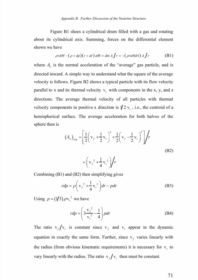
7/30/2019 The Grand Unified-mobilecrackers
http://slidepdf.com/reader/full/the-grand-unified-mobilecrackers 77/143
Appendix B. Further Discussion of the Neutrino Structure
71
Figure B1 shoes a cylindrical drum filled with a gas and rotating
about its cylindrical axis. Summing, forces on the differential element
shown we have( )( ) ( )
n nrd l dp r dr d l dm A r rd drl A r ρ θ ρ θ ρ θ − + + = = − (B1)
wheren
is the normal acceleration of the “average” gas particle, and is
directed inward. A simple way to understand what the square of the average
velocity is follows. Figure B2 shows a typical particle with its flow velocity
parallel to x and its thermal velocity vr with components in the x, y, and z
directions. The average thermal velocity of all particles with thermal
velocity components in positive x direction is 1 2 vr
, i.e., the centroid of a
hemispherical surface. The average acceleration for both halves of the
sphere then is
( )2 2
1 1 1 1v v v v
2 2 2 2n f r f r avg
r ⎡ ⎤⎛ ⎞ ⎛ ⎞
= + + −⎢ ⎥⎜ ⎟ ⎜ ⎟⎝ ⎠ ⎝ ⎠⎢ ⎥⎣ ⎦
(B2)
2 21v v
4 f r
r ⎛ ⎞
= +⎜ ⎟⎝ ⎠
Combining (B1) and (B2) then simplifying gives
2 21v v
4 f r
rdp dr pdr ρ ⎛ ⎞
= + −⎜ ⎟⎝ ⎠
(B3)
Using ( ) 21 3 vr p ρ = we have
2
2
v 13
4v
f
r
rdp pdr ⎛ ⎞
= −⎜ ⎟⎜ ⎟⎝ ⎠
(B4)
The ratio v v f r
is constant since v f
and vr
appear in the dynamic
equation in exactly the same form. Further, since v f
varies linearly with
the radius (from obvious kinematic requirements) it is necessary for vr to
vary linearly with the radius. The ratio v v f r then must be constant.
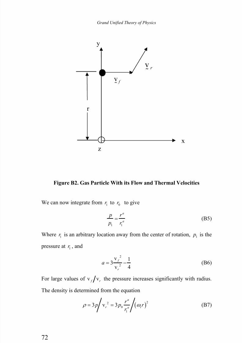
7/30/2019 The Grand Unified-mobilecrackers
http://slidepdf.com/reader/full/the-grand-unified-mobilecrackers 78/143
Grand Unified Theory of Physics
72
Figure B2. Gas Particle With its Flow and Thermal Velocities
We can now integrate from 1r to 0r to give
1 1
a
a
p r
p r = (B5)
Where 1r is an arbitrary location away from the center of rotation, 1 p is the
pressure at 1r , and
2
2
v 13
4v
f
r
a = − (B6)
For large values of v v f r
the pressure increases significantly with radius.
The density is determined from the equation
( )22
0
1
3 v 3a
r t a
r p p r r
ρ ω = = (B7)
y
v r
r
z
x
v f
7/30/2019 The Grand Unified-mobilecrackers
http://slidepdf.com/reader/full/the-grand-unified-mobilecrackers 79/143
Appendix B. Further Discussion of the Neutrino Structure
73
where 1r ω is the thermal velocity (t
ω is the thermal velocity constant of
proportionality). To have a constant density we set 2 0a − = or
3v v 1 4 0 f r − = (B8)
or
v v 3 4 0.866 f r = = (B9)
If v 0.866v f r > and the path is curved then the density will increase with
radius for the steady state rotating drum.
We have shown a possible mechanism for producing curved flow
in a gas. Such a flow could be initiated by a random fluctuation of the
background producing a small curvature then the curvature gets accentuated
by the thermal separation process described here. If such a flow can be
made to exceed the nozzle critical speed which is ( )5 12 v 0.645vr r = 1
then the curved flow could cause a density increase and thus a condensation
of the particles. The thermal separation and the condensation phenomena
are required in the stable state envisioned for this theory. Let us now
investigate flows into a sink then out of the sink. Consider a sphere with
two symmetric holes in it through which air can enter the sphere. Let a
vacuum pump be placed at the bottom of the sphere, see Figure B3. Now
when air is pumped from the sphere air beings flowing in through the two
inlet holes. “Flow smoke” can be introduced separately into each of theholes to visualize the flow for each hole.
It is expected that air will begin swirling about the y-axis
clockwise when viewed looking inward toward the +y axis, because of the
flow curvature required for holes not on the y-axis, and the resulting angular
momentum produced. Figure B3 shows the flow for two holes. It is seen
1 The speed of sound “a” is ( )( ) r 3 v p vc c , where c
pis the specific heat at
constant pressure andvc at constant volume. For air 1.4
vc c p
= so 1.4 3var
= .
For an ideal gas 5 3v
c c p
= and ( )5 3 3 v 0.745va r r = × = .
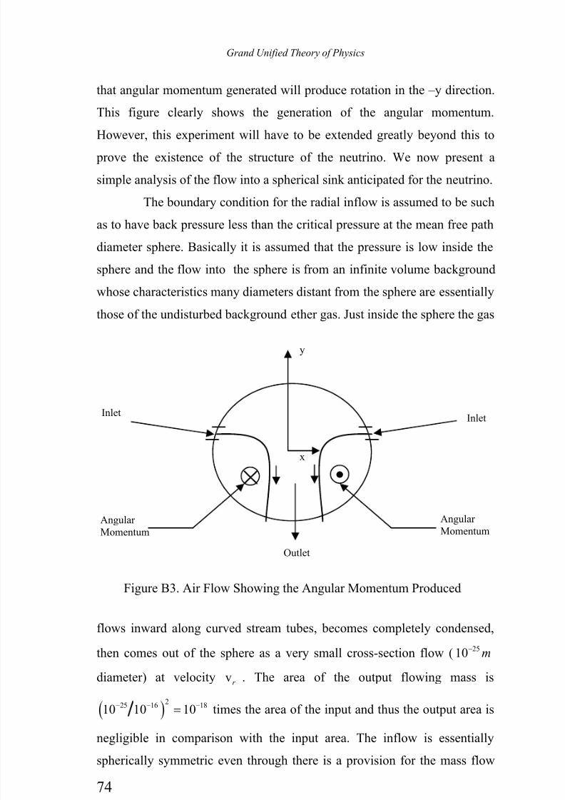
7/30/2019 The Grand Unified-mobilecrackers
http://slidepdf.com/reader/full/the-grand-unified-mobilecrackers 80/143
Grand Unified Theory of Physics
74
that angular momentum generated will produce rotation in the –y direction.
This figure clearly shows the generation of the angular momentum.
However, this experiment will have to be extended greatly beyond this to prove the existence of the structure of the neutrino. We now present a
simple analysis of the flow into a spherical sink anticipated for the neutrino.
The boundary condition for the radial inflow is assumed to be such
as to have back pressure less than the critical pressure at the mean free path
diameter sphere. Basically it is assumed that the pressure is low inside the
sphere and the flow into the sphere is from an infinite volume background
whose characteristics many diameters distant from the sphere are essentially
those of the undisturbed background ether gas. Just inside the sphere the gas
flows inward along curved stream tubes, becomes completely condensed,
then comes out of the sphere as a very small cross-section flow ( 2510 m−
diameter) at velocity vr . The area of the output flowing mass is
( )225 16 1810 10 10− − −= times the area of the input and thus the output area is
negligible in comparison with the input area. The inflow is essentially
spherically symmetric even through there is a provision for the mass flow
Angular Momentum
Angular Momentum
InletInlet
Outlet
x
y
Figure B3. Air Flow Showing the Angular Momentum Produced

7/30/2019 The Grand Unified-mobilecrackers
http://slidepdf.com/reader/full/the-grand-unified-mobilecrackers 81/143
Appendix B. Further Discussion of the Neutrino Structure
75
out to be equal the inflow. This portion of the flow making up the
hypothesized inhomogeneous assemblage is straightforward and its analysis
is simple.A fairly accurate approximation to the inflow is to assume that the
density remains constant down to the mean-free path sphere. Further, we
take the flow velocity to be the sonic velocity which is approximately
( )90.8v 3 10 /m
m s× . Now the input flow m is
( ) 2v 4 0.8vb mm A m l ρ η π = ×
( )66 85 32 910 10 4 4 10 3 10π − −× × × × (B10)
210 /kg s−
A more accurate calculation (accounting for compressibility) can be
performed using a lumped-parameter analysis which consists of writing the
radial (linear) momentum equation, the energy balance, and the mass
balance with the equation of state
2
0 1 3 vr p ρ =
. In the following paragraphs we present the compressible analysis.
The flow of gas into a three dimensional “sink” is the same as the
flow down a conical converging nozzle where the cone half angle is
increased to 180º. The flow of a compressible gas along a converging
nozzle is straightforward. Let us now present the analysis for the flow along
a straight converging nozzle.
The converging nozzle gas flow analysis is presented on pages 298
– 300 of Binder [16]. Considering the case of flow from an ambient source,
when the flow velocity is zero the velocity at the exit is
1
2 1 22
1 1
2v 1
1
k
k p pk
k p ρ
−⎡ ⎤⎛ ⎞⎢ ⎥= − ⎜ ⎟⎢ ⎥− ⎝ ⎠⎢ ⎥⎣ ⎦
(B11)
where k is the specific heat ratiov p
c c which for air is 1.4 and for the hard
particle gas of this theory is 5 3 , 1 p and 1 ρ are the ambient gas pressure
7/30/2019 The Grand Unified-mobilecrackers
http://slidepdf.com/reader/full/the-grand-unified-mobilecrackers 82/143
Grand Unified Theory of Physics
76
and mass density, and 2 p is the exit pressure. As 2 p decreases it reaches a
value which maximizes 2v . This magnitude of pressure is the “critical”
pressure and its value is
1
1
2
1
k
k
c p p
k
−⎛ ⎞= ⎜ ⎟
+⎝ ⎠(B12)
Substituting this as 2 p in (B11) gives the maximum outflow velocity vcas
2 1 1
1 1
22 2v 1
1 1 1c
p k pk
k k k ρ ρ
⎡ ⎤= − =⎢ ⎥− + +⎣ ⎦
(B13)
For the ideal gas with 5 3k = and using11 1 v 3r p ρ = , where
1vr is the
ambient thermal velocity. The velocity becomes
1 1v 5 12v 0.645v
c r r = = (B14)
we note that this maximum velocity is smaller than the speed of sound
( )0.745vr a = since
1
1
5 12vv0.866
5 9v
c r
r a
= = (B15)
The density at the nozzle outlet is computed now.
11
1 1
2
1
k
k c c
k k k
c
p p p
k ρ ρ ρ
−⎛ ⎞= = ⎜ ⎟
+⎝ ⎠(B16)
Thus
1
1
2
1
k
k k k
ck
ρ ρ −⎛ ⎞
= ⎜ ⎟+⎝ ⎠(B17)
or
1
1
1
2
1
k
c
k
ρ ρ −⎛ ⎞
= ⎜ ⎟+⎝ ⎠
(B18)
For the ideal gas
10.650c ρ ρ = (B19)

7/30/2019 The Grand Unified-mobilecrackers
http://slidepdf.com/reader/full/the-grand-unified-mobilecrackers 83/143
Appendix B. Further Discussion of the Neutrino Structure
77
The critical density for air (with k = 1.4) is
10.634c
ρ ρ = (B20)
The requirement that the angular momentum ( )2 for these
assemblages to be always the same implies that the mass inflow rate always
to be one precise value independent of what occurs inside the radius at
which sonic speed occurs. It is clear that this radius must be in the order of
the mean free path. Once such a flow were initiated the mass flow probably
would increase until it is impeded. The impediment would be produced by
background particles from the opposite end of each diameter interfering
with inflow at the other end of the diameter.
It is commonly believed that further inflow beyond the critical
sphere is impossible, since such flow is still converging. We have presented
arguments which might provide a mechanism for further converging flow.
These arguments are based on the flow taking a curved path which results in
higher (total) speed particles moving toward a larger radius path. Thecurved paths may provide thermal separation and thus may permit further
converging flow. For the time being we will assume that further flow is
possible and that it results in complete condensation.
First we assume a spherically symmetric inflow and then
determine the diameter of the sphere at which complete condensation occurs.
The mass inflow at the sonic radius is
( ) 2v 4 0.8vb mm A m l ρ η π = = × (B21)
and at the completely condensed radiusv
r is
( )24 v solid v mm r ρ π = × (B22)
where we assume that the particles are flowing in at the background mean
speed vm
. Now
( )34 3
b
solid
b
m
r ρ
π = (B23)
Using ρ from above and equating m from (B21) to (B22) gives
7/30/2019 The Grand Unified-mobilecrackers
http://slidepdf.com/reader/full/the-grand-unified-mobilecrackers 84/143
Grand Unified Theory of Physics
78
( )1 23 264 3 0.8 3 10 .
v br r l mπ η
−⎡ ⎤ ×⎣ ⎦ (B24)
The next step in the analysis, which we have not taken, is let the
assemblage move at the velocity v vr m− and then try to fit stream-like into
the spherical volume subject to the following conditions:
1. The tubes fill the volume down to a pre-selected cylindrical core.
2. The tubes and radius are selected so that no friction results
between the tubes.
3. The flow produces an angular momentum of 2 about the core
cylindrical axis.
4. The flow is all turned so that it is directed axially along the
cylindrical axis in the direction of the cylindrical core translation
(and at velocity v vr m
− ).
5. The flow also must apply a thrust to the side of the cylindrical core
equal to the proton thrust ( 610 Newtons).
The last step in the analysis is to determine the size of the
cylindrical solid core. Hopefully some additional insight into the core
geometry will come from the above analysis. (We have made
approximations of its size if it were spherical.) The flow into the aft end of
the core would be at velocity vm
. The axial thrust on the side would
increase this velocity to vr as the final condensation takes place. The mass
and energy conservation equations for the core are straight forward. Assume
that all the particles entering the core are a sample of the background gas
and that they are all aligned parallel to each other, but not touching each
other. Let the particles be accelerated from velocity vm
to vr
by the side
thrusting force while the final condensation takes place. The mass flow rate
in is m
, at velocity vm , the mass flow rate out is m
at v ,r and the mass
continuity equation is ( )in
ρ ( )v vm r out A ρ = . The energy balance is
( )( )1 2in
ρ ( )( )2 2v v 1 2 v vm r r r out A ρ = (B25)
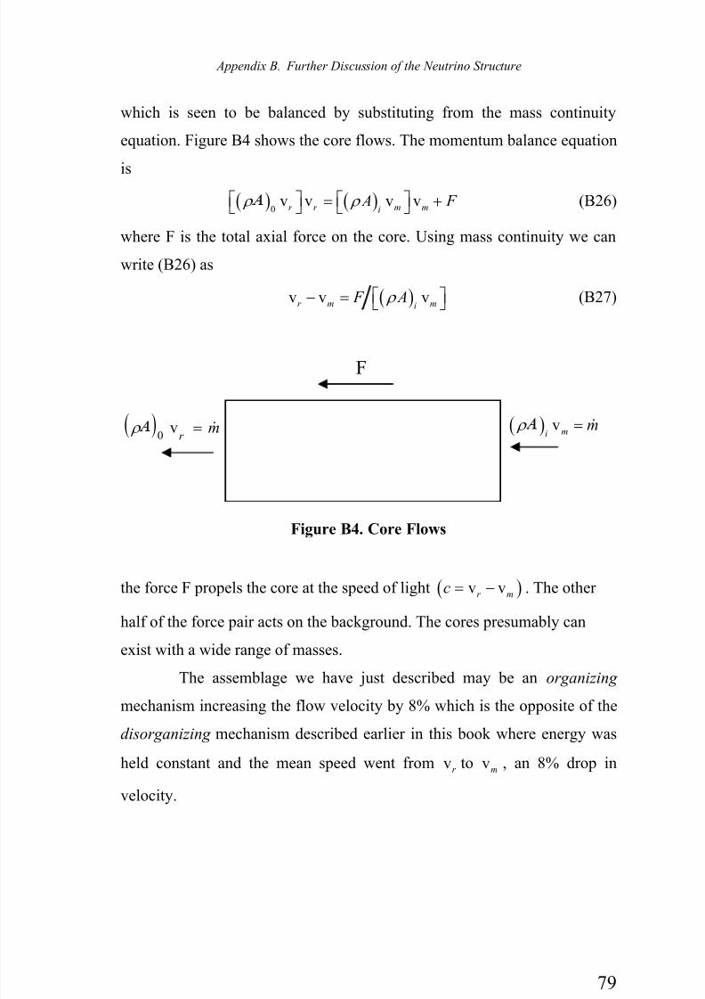
7/30/2019 The Grand Unified-mobilecrackers
http://slidepdf.com/reader/full/the-grand-unified-mobilecrackers 85/143
Appendix B. Further Discussion of the Neutrino Structure
79
which is seen to be balanced by substituting from the mass continuity
equation. Figure B4 shows the core flows. The momentum balance equation
is
( ) ( )0
v v v vr r m mi
A F ρ ρ ⎡ ⎤ ⎡ ⎤= +⎣ ⎦ ⎣ ⎦ (B26)
where F is the total axial force on the core. Using mass continuity we can
write (B26) as
( )v v vr m mi
F A ρ ⎡ ⎤− = ⎣ ⎦ (B27)
Figure B4. Core Flows
the force F propels the core at the speed of light ( )v vr m
c = − . The other
half of the force pair acts on the background. The cores presumably can
exist with a wide range of masses.
The assemblage we have just described may be an organizing
mechanism increasing the flow velocity by 8% which is the opposite of the
disorganizing mechanism described earlier in this book where energy was
held constant and the mean speed went from vr to vm
, an 8% drop in
velocity.
F
( )0
vr
m ρ = ( ) vmi
m ρ =
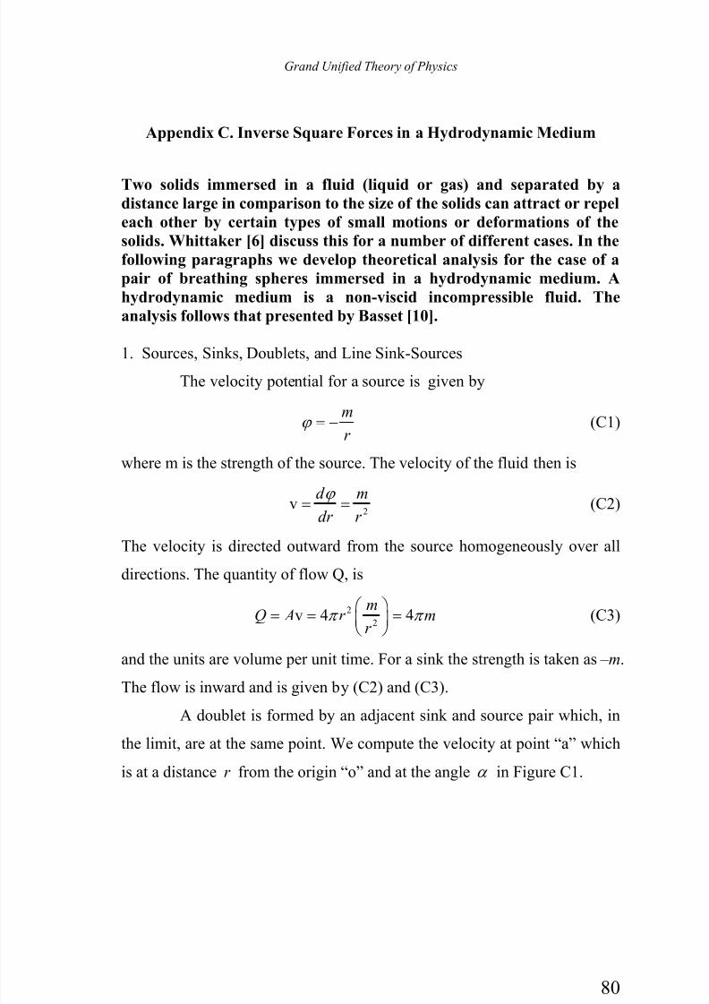
7/30/2019 The Grand Unified-mobilecrackers
http://slidepdf.com/reader/full/the-grand-unified-mobilecrackers 86/143
Grand Unified Theory of Physics
80
Appendix C. Inverse Square Forces in a Hydrodynamic Medium
Two solids immersed in a fluid (liquid or gas) and separated by a
distance large in comparison to the size of the solids can attract or repel
each other by certain types of small motions or deformations of the
solids. Whittaker [6] discuss this for a number of different cases. In the
following paragraphs we develop theoretical analysis for the case of a
pair of breathing spheres immersed in a hydrodynamic medium. A
hydrodynamic medium is a non-viscid incompressible fluid. The
analysis follows that presented by Basset [10].
1. Sources, Sinks, Doublets, and Line Sink-Sources
The velocity potential for a source is given by
m
r ϕ = − (C1)
where m is the strength of the source. The velocity of the fluid then is
2v
d m
dr r
ϕ = = (C2)
The velocity is directed outward from the source homogeneously over all
directions. The quantity of flow Q, is
2
2v 4 4
mQ A r m
r π π
⎛ ⎞= = =⎜ ⎟
⎝ ⎠(C3)
and the units are volume per unit time. For a sink the strength is taken as –m.
The flow is inward and is given by (C2) and (C3).
A doublet is formed by an adjacent sink and source pair which, in
the limit, are at the same point. We compute the velocity at point “a” which
is at a distance r from the origin “o” and at the angle α in Figure C1.
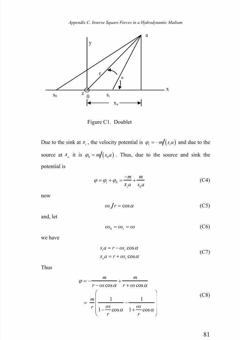
7/30/2019 The Grand Unified-mobilecrackers
http://slidepdf.com/reader/full/the-grand-unified-mobilecrackers 87/143
Appendix C. Inverse Square Forces in a Hydrodynamic Medium
81
Due to the sink ati, the velocity potential is ( )i i
m s aϕ = − and due to the
source ato
it is ( )0 0m s aϕ = . Thus, due to the source and sink the
potential is
0
0
i
i
m ma s a
ϕ ϕ ϕ −= + = + (C4)
now
cosi
os r α = (C5)
and, let
0 ios os os= = (C6)
we have
cos
cos
i i
o i
s a r os
s a r os
α
α
= −
= +(C7)
Thus
cos cos
1 1
1 cos 1 cos
m m
r os r os
mos osr
r r
ϕ α α
α α
= − +− +
⎛ ⎞
⎜ ⎟= −⎜ ⎟⎜ ⎟− +⎜ ⎟⎝ ⎠
(C8)
α
x
y
r
a
z0 si s0
Figure C1. Doublet
xa

7/30/2019 The Grand Unified-mobilecrackers
http://slidepdf.com/reader/full/the-grand-unified-mobilecrackers 88/143
Grand Unified Theory of Physics
82
For small values of os r we have
2
1 cos 1 cos
cos
m os os
r r r
os
r
ϕ α α
α
⎛ ⎞= + − −⎜ ⎟⎝ ⎠
=
(C9)
Let m increase indefinitely and os decrease indefinitely but with the
product remaining constant at the magnitude then
3cos a
r r
µ ϕ α 2= = (C10)
wherea
x is the x coordinate of the point “a”.
The velocity potential due to a sheet of doublets with strength
“m” per unit of surface area where the doublet axis is in the direction
of the normal to the sheet is given by
cosm
dsr
εµ
ϕ 2= −∫∫ (C11)
where ε is the angle from the normal. Integrating (C11) gives
md ϕ = − Ω∫∫ (C12)
where Ω is the solid angle (in sterradians). For a constant value of m
mϕ = − Ω (C13)
When the area is a narrow long rectangle along the z-axis Laplace’sequation (of continuity) becomes
10
d d
r dr dr
ϕ ϕ 2
2+ = (C14)
The solution of (C14) is
lnm r ϕ = (C15)
and
vd m
dr r
ϕ = = (C16)
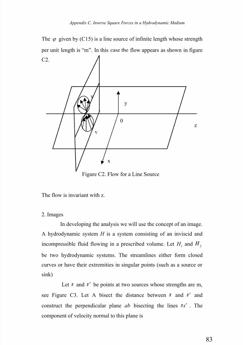
7/30/2019 The Grand Unified-mobilecrackers
http://slidepdf.com/reader/full/the-grand-unified-mobilecrackers 89/143
Appendix C. Inverse Square Forces in a Hydrodynamic Medium
83
The ϕ given by (C15) is a line source of infinite length whose strength
per unit length is “m”. In this case the flow appears as shown in figure
C2.
The flow is invariant with z.
2. Images
In developing the analysis we will use the concept of an image.
A hydrodynamic system H is a system consisting of an inviscid and
incompressible fluid flowing in a prescribed volume. Let 1 H and 2
be two hydrodynamic systems. The streamlines either form closed
curves or have their extremities in singular points (such as a source or
sink)
Let and ′ be points at two sources whose strengths are m,
see Figure C3. Let A bisect the distance between and ′ and
construct the perpendicular plane ab bisecting the lines s′ . The
component of velocity normal to this plane is
v
v
0 z
y
x
Figure C2. Flow for a Line Source
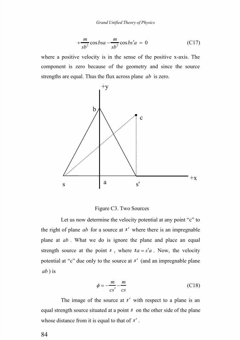
7/30/2019 The Grand Unified-mobilecrackers
http://slidepdf.com/reader/full/the-grand-unified-mobilecrackers 90/143
Grand Unified Theory of Physics
84
cos cosm m
bsa bs a sb sb2 2
′+ − = 0 (C17)
where a positive velocity is in the sense of the positive x-axis. Thecomponent is zero because of the geometry and since the source
strengths are equal. Thus the flux across plane ab is zero.
Let us now determine the velocity potential at any point “c” to
the right of plane ab for a source at ′ where there is an impregnable
plane at ab . What we do is ignore the plane and place an equal
strength source at the point , where a s a′= . Now, the velocity
potential at “c” due only to the source at ′ (and an impregnable plane
ab ) is
m m
cs csφ = − −
′(C18)
The image of the source at ′ with respect to a plane is an
equal strength source situated at a point on the other side of the plane
whose distance from it is equal to that of ′ .
+y
b
c
as s' +x
Figure C3. Two Sources
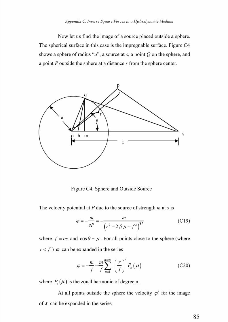
7/30/2019 The Grand Unified-mobilecrackers
http://slidepdf.com/reader/full/the-grand-unified-mobilecrackers 91/143
Appendix C. Inverse Square Forces in a Hydrodynamic Medium
85
Now let us find the image of a source placed outside a sphere.
The spherical surface in this case is the impregnable surface. Figure C4
shows a sphere of radius “a”, a source at s, a point Q on the sphere, anda point P outside the sphere at a distance r from the sphere center.
The velocity potential at P due to the source of strength m at s is
( )1 2
2
m m
sP r fr f
ϕ
µ 2 2
= − = −
− +
(C19)
where f os= and cosθ µ = . For all points close to the sphere (where
r f < ) ϕ can be expanded in the series
( )1
nn
n
n
m m r
f f f P ϕ µ
=∞
=
⎛ ⎞= − − ⎜ ⎟
⎝ ⎠∑ (C20)
where ( )n P is the zonal harmonic of degree n.
At all points outside the sphere the velocity ϕ ′ for the image
of can be expanded in the series
r
q
p
s
f
a
o h m
Figure C4. Sphere and Outside Source
θ

7/30/2019 The Grand Unified-mobilecrackers
http://slidepdf.com/reader/full/the-grand-unified-mobilecrackers 92/143
Grand Unified Theory of Physics
86
1
1nn
n n
n
a P
r r ϕ
=∞
=
⎛ ⎞′ = ⎜ ⎟⎝ ⎠
∑ (C21)
With the sphere at rest for a r =
0d d
dt dt
ϕ ϕ ′+ = (C22)
since no flux goes through the sphere. From (C20), (C21), and (C22)
1
1
1 1
10
n nn
n n nn
n n
na nm P A P
f R
=∞ =∞−
+ 2= =
++ =∑ ∑ (C23)
From (C23) 0 0 A = and1
1
n
n
mn a A
n f
+⎛ ⎞
= − ⎜ ⎟+ ⎝ ⎠
(C24)
and
( )
2 1
11
1 11 1
1
1
nn
nnn
n nn n nnn n
n n
n am P
n fr
P ma c ma c P f f nr r
ϕ +=∞
+=
=∞ =∞
+ += =
′ = −+
= − ++
∑
∑ ∑
(C25)
where
c a f 2= (C26)
For c r < (or a fr 2 < ) and using the dummy variable x c< we have
( )
1
00 12
n
n
n
nc P d c
r nr r
λ
λ µ λ
+
2 2=
=∞ ⎛ ⎞
= ⎜ ⎟ +− + ⎝ ⎠∑∫(C27)
by adding and subtracting ( )ma fr from (C25) ϕ ′ is
( ) ( )1 2 1 2
1 1
2 2
ma ma
f f r rc c r r ϕ
µ λµ λ 2 2 2 2′ = − +
− + − +(C28)
The first term is a point source of strength ma f located at where
OH c a f 2= = and the second term is a line sink with strength m a
per unit of length. The sink extends from H to O .
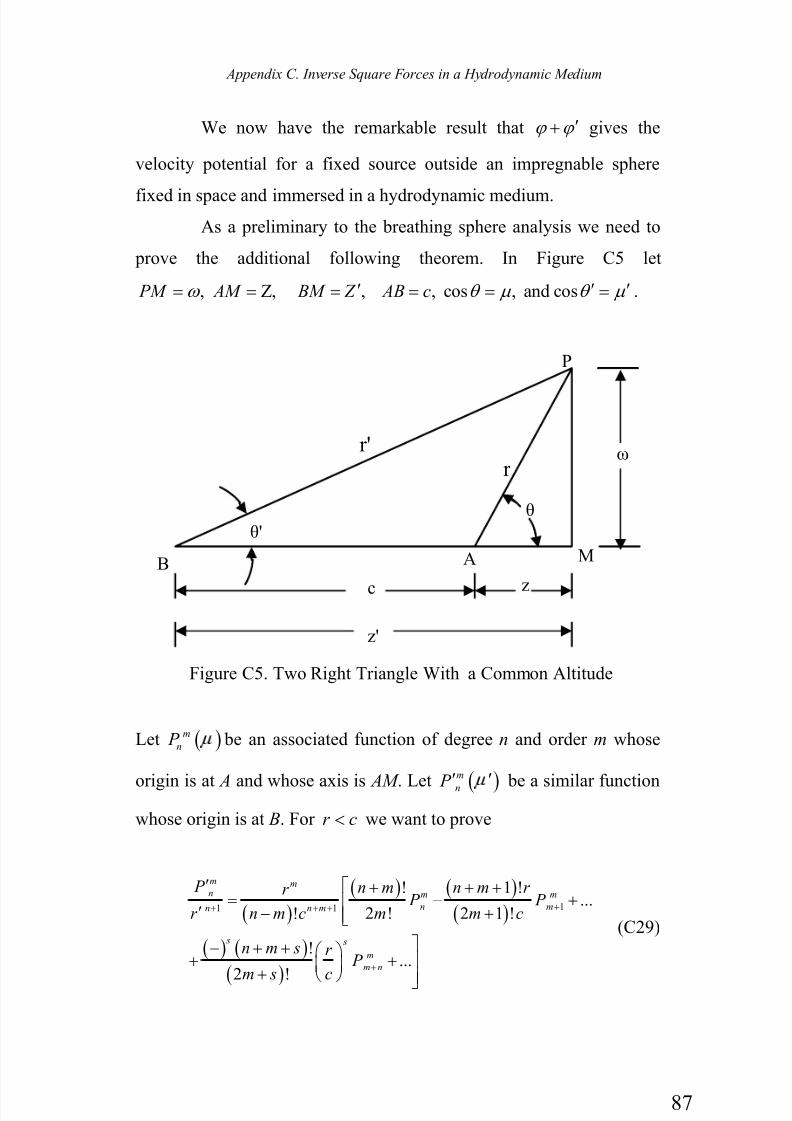
7/30/2019 The Grand Unified-mobilecrackers
http://slidepdf.com/reader/full/the-grand-unified-mobilecrackers 93/143
Appendix C. Inverse Square Forces in a Hydrodynamic Medium
87
We now have the remarkable result that ϕ ϕ ′+ gives the
velocity potential for a fixed source outside an impregnable sphere
fixed in space and immersed in a hydrodynamic medium.
As a preliminary to the breathing sphere analysis we need to
prove the additional following theorem. In Figure C5 let
, , PM AM ω = = Ζ , BM Z ′= , cos , and cos AB c θ µ θ µ ′ ′= = = .
Let ( )m
n P be an associated function of degree n and order m whose
origin is at A and whose axis is AM . Let ( )m
n P ′ ′ be a similar function
whose origin is at B. For r c< we want to prove
( )
( ) ( )
( )
( ) ( )
( )
11 1
! 1 !...
2 ! 2 1 !!
!...
2 !
m mn m m
n mn n m
s s
m
m n
P n m n m r r P P
m m cr n m c
n m s r P
m s c
++ + +
+
′ ⎡ + + += − +⎢
′ +− ⎢⎣
⎤− + + ⎛ ⎞+ + ⎥⎜ ⎟+
⎝ ⎠ ⎥⎦
(C29)
r'
P
ω
B
θ'
r
A M
c z
z'
Figure C5. Two Right Triangle With a Common Altitude
θ
7/30/2019 The Grand Unified-mobilecrackers
http://slidepdf.com/reader/full/the-grand-unified-mobilecrackers 94/143
Grand Unified Theory of Physics
88
and for r c′ <
( )
( )
( ) ( )
( )( )
( )
11 1
! 1 !
2 ! 2 1 !!
!...
2 !
n m m mn m m
n mn n m
s
m
m n
P n m n mr r P P
m m cr n m c
n m s r P
m s c
−
++ + +
+
⎡− + + +′ ′′ ′= + +⎢
+− ⎢⎣⎤+ + ′⎛ ⎞ ′+ + ⎥⎜ ⎟+ ⎝ ⎠ ⎥⎦
(C30)
To begin this proof we start with the equations (taken from
Jahnke [25])
( ) ( )( )2
1 1
m
nm
n m
d P P
d
µ µ µ µ µ
µ
2= − < (C31)
and
( ) ( )2
1 1m
mn n
m m
d P P v v v
dv
2= − > (C32)
wheren
P is a zonal harmonic or Legendre’s coefficient (for the
solution of the Legendre differential equation). The valuen
P can be
written in the form of the definite integral (following Basset [27])
0
11cos
m
n P d
π µ θ θ
π
2= + −∫ (C33)
or, as
1
0
11cos
n
n P d
π µ θ θ
π
− −2= + −∫ (C34)
An expression for m
n P will be obtained now. Let
2
1
sin
0 1cos
m
m n m
d V
π θ θ
µ µ θ + +
2
=⎡ ⎤+ −⎣ ⎦
∫ (C35)
Differentiating with respect to
7/30/2019 The Grand Unified-mobilecrackers
http://slidepdf.com/reader/full/the-grand-unified-mobilecrackers 95/143
Appendix C. Inverse Square Forces in a Hydrodynamic Medium
89
( )
2
2
2
11
1 cos sin1
1 0 1cos
1 cos sin1
1 0 1cos
m
m
n m
m
mn m
d dV n m
d
n m d n m V
π µ µ θ θ θ
µ µ µ µ θ
π θ θ θ
µ µ µ θ
2
+ +2 2
++ +2 2
− + ++ += −
− + −
+ += − − + +
− + −
∫
∫(C36)
Integrating by parts
( )( )1
1
2 1
m
m
n m n mdV V
d mµ +
+ + −= −
+(C37)
Since0 m
V P π = we have
( )( ) ( )
( )
1 2
1 3 5 2 1
m
nmm
n m n m n md P V
d mπ µ
− + − + −= −
−i i
(C38)
From this
( ) ( )
( ) ( )
2 2
1
! 1 sin
! 3 5 2 1 0 1cos
m mm
n n m
n m d P
n m m
π µ θ θ
π µ µ θ
2
+ +
2
+ −=
− 1 − + −
∫i i
(C39)
Using the transformation
cos 1cos
1cos
µ ϕ µ θ
µ ϕ
2
2
+ −=
+ −(C40)
We get
( ) ( )( ) ( ) 2
2
! 11cos sin
! 3 5 2 1 0
mn m
m mn
n m P d
n m m
π µ
µ ϕ ϕ ϕ π
2−
2
+ −= − −− 1 − ∫i i
(C41)
We have just proved that m
n P can be expressed in either of the two forms,
(C41)
( )2
2
01 1cos sin
n mmm m
n P m d π
µ µ ϕ ϕ ϕ −
2 2⎡ ⎤= − − −⎣ ⎦∫ (C42)
or, (C39)

7/30/2019 The Grand Unified-mobilecrackers
http://slidepdf.com/reader/full/the-grand-unified-mobilecrackers 96/143
Grand Unified Theory of Physics
90
( )
22
10
sin1
1cos
mm
m
n n m
d P m
π ϕ ϕ µ
µ µ ϕ
2
+ +2
= −+ −
∫ (C43)
where
( )
( ) ( )
!
! 3 2 1
n m M
n m m π
+=
− 1 −i
(C44)
Using this we can write (C42) as
( )
( )
( )
2
1 2
2
2
sin
cos0
sin
0 1cos
m mn m
n n m
mm
n m
P d m
r z i
d m
c r
π µ ϕ ϕ
ω ϖ ϕ
π ϕ ϕ ω
µ µ ϕ
+ + +
+ +2
′ ′=
′ ′ +
=
+ + −
∫
∫(C45)
We let
1cosλ µ µ ϕ 2= + − (C46)
then, for r < c
( ) ( ) ( )( )
( ) ( ) ( )
1 1
2
1 21 1
2!0
1sin
!
m mn
n n m
s
m
P n m n mm r r n m
c cr c
n m n m s r d
s c
π µ ω λ λ
λ ϕ ϕ
2
+ + +⎧′ ′ + + + +⎪ ⎛ ⎞= − + + + +⎨ ⎜ ⎟′ ⎝ ⎠⎪⎩
⎫− + + + + ⎪⎛ ⎞+ + ⎬⎜ ⎟
⎝ ⎠ ⎪⎭
∫
(C47)
Using the first form of m
n P , (C42) we find
( )
( )
( ) ( )
( )
( ) ( )
( )
11 1
! 1 !
2 ! 2 1 !!
!
2 !
m mn m m
m mn n m
s s
m
m s
P n m n mr r P P
m m cr n m c
n m s r P
m s c
µ
++ + +
+
′ ′ ⎡ + + += − +⎢
′ +− ⎢⎣
⎫− + + ⎪⎛ ⎞+ ⎬⎜ ⎟+ ⎝ ⎠ ⎪⎭
(C48)
Further, for r c′ < we change θ and θ ′ to their supplements and since
( ) ( )cos cosn mm m
n n P P π θ θ −
− = − (C49)
7/30/2019 The Grand Unified-mobilecrackers
http://slidepdf.com/reader/full/the-grand-unified-mobilecrackers 97/143
Appendix C. Inverse Square Forces in a Hydrodynamic Medium
91
we obtain
( ) ( )
( )
( )
( )
( )
( )
( )
1 1
1
1 !
2 !!1 !
2 1 !
!
2 !
n m m mn m
mn n m
m
m
s
m
m s
P n mr P
mr n m cn m r
P m c
n m s r P
m s c
µ −
+ + +
+
+
− +⎡′′= ⎢
− ⎣+ + ′
′+ ++
+ + ′⎛ ⎞ ′+ ⎜ ⎟+ ⎝ ⎠
(C50)
3. The Force of Interaction of Two Breathing Spheres
Let us now consider two spheres A and B immersed in a
hydrodynamic medium. The spheres are configured so that they can
expand and contract sinuosidally, but always remains spherical. Such
spheres are called breathing spheres. Our object is to determine the force
of interaction between two such spheres.
Let 1ϕ be the velocity potential of the medium where sphere A
pulsates and where sphere B doesn’t. Similarly let 2ϕ be the velocity
potential when B pulsates and A doesn’t. The velocity potential when
both pulsate is
1 2ϕ ϕ ϕ = + (C51)
The radius of A is a and B is b. If B were not present the value of 1ϕ
would be
1 a a r ϕ 2= − (C52)
which can be seen from differentiating 1ϕ . Thus
1va a
r
2
2=
(C53)
Where r a= , 1v a= , as required, and the velocity is an inverse square
value as required. This is the velocity due to a source of strength a a2
located at the center of A.
7/30/2019 The Grand Unified-mobilecrackers
http://slidepdf.com/reader/full/the-grand-unified-mobilecrackers 98/143
Grand Unified Theory of Physics
92
The image of this flow in B will be a source of strength
a b a c2 at the inverse point P coupled with a line sink extending from
the inverse point P to the center B. Its strength is a a b2 per unit length.
Using
m a b a c
f b c
2
2
=
=
(C54)
the strength of the source at P is m and of the line sink from B to P is
m f − per unit length. The image of these in A is given similarly, see
(C50). Thus 1ϕ and 2ϕ will be the potentials of two infinite systems of
sources and line sinks which lie within each sphere, respectively.
Let 2 F be the resultant force of the pressure of the liquid on B
toward A. Now
2
0
cos
1 sin22
F p ds
b V d π
θ
πρ ϕ θ θ 2 2
= −
⎛ ⎞′= +⎜ ⎟⎝ ⎠
∫∫
∫(C55)
where ρ is the density of the medium, b is the radius of sphere B, and V
is the velocity of the fluid at the surface of B (1 2 V ρ 2 is the dynamic
pressure). Let
0
0
sin2
sin2
P d
Q d
π
π
ϕ θ θ
ϕ θ θ 2
=
=
∫
∫(C56)
then
0sin2 d P
π
ϕ θ θ =∫ (C57)
In order to find the portion of 2 F which depends upon V 2 let
v b b
2=
then
( ) ( )4v 1V b b d d ϕ θ 22 2 2= + (C58)
7/30/2019 The Grand Unified-mobilecrackers
http://slidepdf.com/reader/full/the-grand-unified-mobilecrackers 99/143
Appendix C. Inverse Square Forces in a Hydrodynamic Medium
93
Since v is constant over the surface of B (due to our assumed breathing
sphere configuration) the portion of 2 F depending upon it is zero.
Letting the portion of the pressure depending upon V 2 be I we have
0
0
0
0
0
1 1v sin 2 sin 2
2 2
1sin 2 cos 2
2
1 12 sin 2
2 2
d I b d d
d
d d d
d d
d d
d
π
π
π
π
π
ϕ πρ θ θ πρ θ θ
θ
ϕ ϕ πρ ϕ θ θ θ
θ θ
ϕ πρ ϕ ϕ θ θ πρ ϕ
θ
2
2 2
2 2
2
22
2
⎛ ⎞= = ⎜ ⎟
⎝ ⎠
⎛ ⎞= − +⎜ ⎟
⎝ ⎠
⎛ ⎞⎡ ⎤= − + −⎜ ⎟ ⎣ ⎦
⎝ ⎠
∫ ∫
∫
∫
(C59)
From the Laplace continuity equation
2 cotd d d d
b bdr d d dr
ϕ ϕ ϕ ϕ
θ θ
2 22
2 2− = + + (C60)
In this equation we set r b= after differentiating. Thus
vd
dr b
ϕ 2
= (C61)
and
2
00
1 2v 12 sin 2 2cos
2 2
d d I b
b d dr
π π ϕ ϕ πρ ϕ ϕ θ θ πρ ϕ
θ
22 2
2
⎧ ⎫⎛ ⎞⎪ ⎪⎡ ⎤= + − + −⎨ ⎬⎜ ⎟ ⎣ ⎦
⎪ ⎪⎝ ⎠⎩ ⎭
∫
(C62)
Also
00 0 02 cos sin 2
d d Q
d
π π π π ϕ θϕ θ ϕ θ ϕ ϕ
θ
2 2 2 2⎡ ⎤ ⎡ ⎤= + = +⎣ ⎦ ⎣ ⎦
∫ ∫ (C63)
And
0 0
1 v 1sin 2 sin 2
2 2
d d d Qd d
dr dr b dr
π π ϕ ϕ ϕ θ θ θ θ
2 2 2 2 2
2 2 2 2
⎛ ⎞= − =⎜ ⎟
⎝ ⎠
∫ ∫ (C64)
From this
1 2v 1
2 2
d Q I Q b
b dr πρ ρ
22
2
⎛ ⎞= − +⎜ ⎟
⎝ ⎠(C65)
7/30/2019 The Grand Unified-mobilecrackers
http://slidepdf.com/reader/full/the-grand-unified-mobilecrackers 100/143
Grand Unified Theory of Physics
94
And, when r b=
2
v 1 1
2 4
d Q F b P P Q b
b dr
πρ 2
2 2
2
⎛ ⎞= + − +⎜ ⎟
⎝ ⎠
(C66)
Let 1 P be the part of P due to 1ϕ then if n
is the strength of
any image whose distance from B is r , the portion of 1 P due to this is
( ) ( )1 2
02 sin cos 2 cosd b r br
π
µ θ θ θ θ 2 2− + −∫ and this integral is
( )4 3nb r µ 2− if r b> and ( )4 3
nr bµ 2− if r b< .
If m
is the strength of the nth source image in A from A, and
n ρ ′ that of the other extremity of the line sink image, the part of 1 P due
ton
is
( ) ( )( )
( )( ) ( )
4 4
33
43
n n
n
n n n
n n n
n n
nb bdx X
c c x
bc c
ρ
ρ
µ µ
ρ ρ ρ
µ ρ ρ ρ ρ
2 2
2
′= − +
′− − −
′−= −′− −
∫(C67)
Letn
v be the strength of the nth image in B,nσ ,
nσ ′ the distances of its
extremities from B, then the part of 1 P due to nv is
( )
( )24 4
33 3
n
n
n n nn n n
n
n n
vv v xdx X
b b b
σ
σ
σ σ σ
σ σ 2 2 2′
′−′ = − + = −
′−∫ (C68)
Now
n
n n n
n n n
b b bv
c c c
µ σ σ
ρ ρ ρ
2 2
′= = =′− − −
(C69)
Thus
( )
( ) ( )
2
3
n n n
n
n n
b X
c c
µ ρ ρ
ρ ρ 2
′−′ = −
′− −(C70)
Adding (C47) and (C48) and summing for all integral values of n from
∞ to 0 gives

7/30/2019 The Grand Unified-mobilecrackers
http://slidepdf.com/reader/full/the-grand-unified-mobilecrackers 101/143
Appendix C. Inverse Square Forces in a Hydrodynamic Medium
95
( )
( ) ( )1
0
2n n n
n n
n
n
b P
c c
µ ρ ρ
ρ ρ 2
=∞
=
′−= −
′− −∑ (C71)
In order to find the portion 2 P of P due to 2ϕ it must be
recognized that the original source now is in B. Letnσ ,
nσ ′ be the
distances of the extremities of the nth image in B from B, due to 2ϕ ,
then expressing nµ , nσ , and nσ ′ in terms of nv , nσ , and nσ ′ gives
( )2
0
2n n n
n
n
v P
b
σ σ 2
=∞
=
′−= − ∑ (C72)
and
( )
( ) ( )
( )
0 0
2 2n n n n n n
n n
n n
n n
b v P
bc c
ρ ρ σ σ
ρ ρ 2 2
=∞ =∞
= =
′ ′− −= − −
′− −∑ ∑ (C73)
where n , n ρ , and n ρ ′ refer to the images of A’s motion, and nγ , nσ ,
and nσ ′ to those of B’s motion. We now calculate the following values
( )
( )
( )( )
0 0
1 1
2 2
0 0
a c a
cc b
a c c a b a c a
c c a bc b a c
ρ ρ
ρ ρ
ρ ρ
2 2
2 2
2 2 2 2 2 2 2
2 2 2 22 2 2 2
′= =
′= =−
− − −′= =
− −− −
(C74)
also, if 1m is the mass of the liquid displaced by A we obtain
( )
( )
1 10 1
12
4 4
4
m abma a
c b
a b m
c b a c
µ µ π π
µ
π
2
2 2
2 2
22 2 2 2
= = =−
=− −
(C75)
The 'v s and 'σ can be obtained by symmetrically
interchanging “a” and “b” and putting 2m for m . If we write 2 , 2 N
for the two series in the right-hand side of (C53) we find

7/30/2019 The Grand Unified-mobilecrackers
http://slidepdf.com/reader/full/the-grand-unified-mobilecrackers 102/143
Grand Unified Theory of Physics
96
( ) ( )
( ) ( ) ( )
3 3
6 6
12 1
2
4
a b
c a c a b
a b
c a b c c b a c a a b
m b M
cπ 22 2 2 2 2
22 22 2 2 2 2 2 2 2 2 2 2
2+
− − −
+
− − − − + +
⎡⎢=⎢⎣
⎤⎥
+ ⎥⎡ ⎤ ⎥⎣ ⎦ ⎦
(C76)
( ) ( ) ( )
3 33
22
1
4
a b
c a c a b c a b c
m a b N
cπ 2 22 2 22 2 2 2 2 2 2
+ +− − − − −
⎡ ⎤⎢ ⎥= ⎢ ⎥⎢ ⎥⎣ ⎦
(C77)
and
( )2 22 P M N = − + (C78)
We see that 2 is of the order 2c− and 2 N of the order 5c− .
The value of the portion of 2 F which depends on the square of
the velocity is more difficult to obtain. We will obtain an approximate
value for terms with c to exponents to -5. Let , v ,u a a b b2 2= = and let
n P be zonal harmonics when the origin is at A and the axis is BA.
Similarly, n P ′ are the zonal harmonics when the origin is at B.
Near the surface of B
( )
2 1
1 1
1
Constant
1
nn
n nn
n
n
b A R P
n R
ϕ +
+
=∞
=
⎧ ⎫⎪ ⎪′= + +⎨ ⎬
+⎪ ⎪⎩ ⎭
∑ (C79)
and
( )
2 1
2 1
1
vConstant
1
nn
n nn
n
n
b B R P
R n Rϕ
+
+
=∞
=
⎧ ⎫⎪ ⎪′= − + + +⎨ ⎬
+⎪ ⎪⎩ ⎭∑ (C80)
Omitting the primes for the present and writing nC for the
coefficient of 2
n P in the expression for ϕ we obtain
( )1
12 n nQ C P d µ
2
−= ∑∫ (C81)

7/30/2019 The Grand Unified-mobilecrackers
http://slidepdf.com/reader/full/the-grand-unified-mobilecrackers 103/143
Appendix C. Inverse Square Forces in a Hydrodynamic Medium
97
Since 2
n P is unchanged when − is written for we have
1
10
n P d µ µ 2
−=∫ (C82)
So that
1
14
m n m nQ C C P P d µ
−= ∑ ∫ (C83)
where the summation extends to all positive integral values of m , n
except for m n= . Let
1
m n P P d
µ Φ = ∫ (C84)
Then
1 1 1 1
1 1 1 1m n m n P P d P P d d d µ µ µ µ
− − − −= + Φ = Φ∫ ∫ ∫ ∫ (C85)
From Ferrers [26] we have
( ) ( )
( )( )
( ) ( )
1 1
1 1
11
1 2 1
1
2 1
m n n
n m m
n n P P P
m n m n n
m m P P P
m
+ −
+ −
+⎧⎪Φ = −⎨
− + + +⎪⎩
+ ⎫⎪− − ⎬+ ⎪⎭
(C86)
Thus1
1d µ
−Φ∫ is zero unless 1m n= + or 1n − and in these cases the
integral is (for 1m n= + )
( )
( )( )
1
1
2 1
2 1 2 3
md
m m
µ −
+Φ =
+ +∫ (C87)
(for 1n − )
( ) ( )
1
1
2
2 1 2 1
md
m mµ
−Φ =
− +∫ (C88)
Putting 0,m r R′= = into (8) and (10) we have
( ) ( )( )1 20
1 1 2 2
1 1 2
2!
n
n n n n
n Pr n n P r P P
R c c c
2
+ + + +
+ + +′= − + − (C89)
and
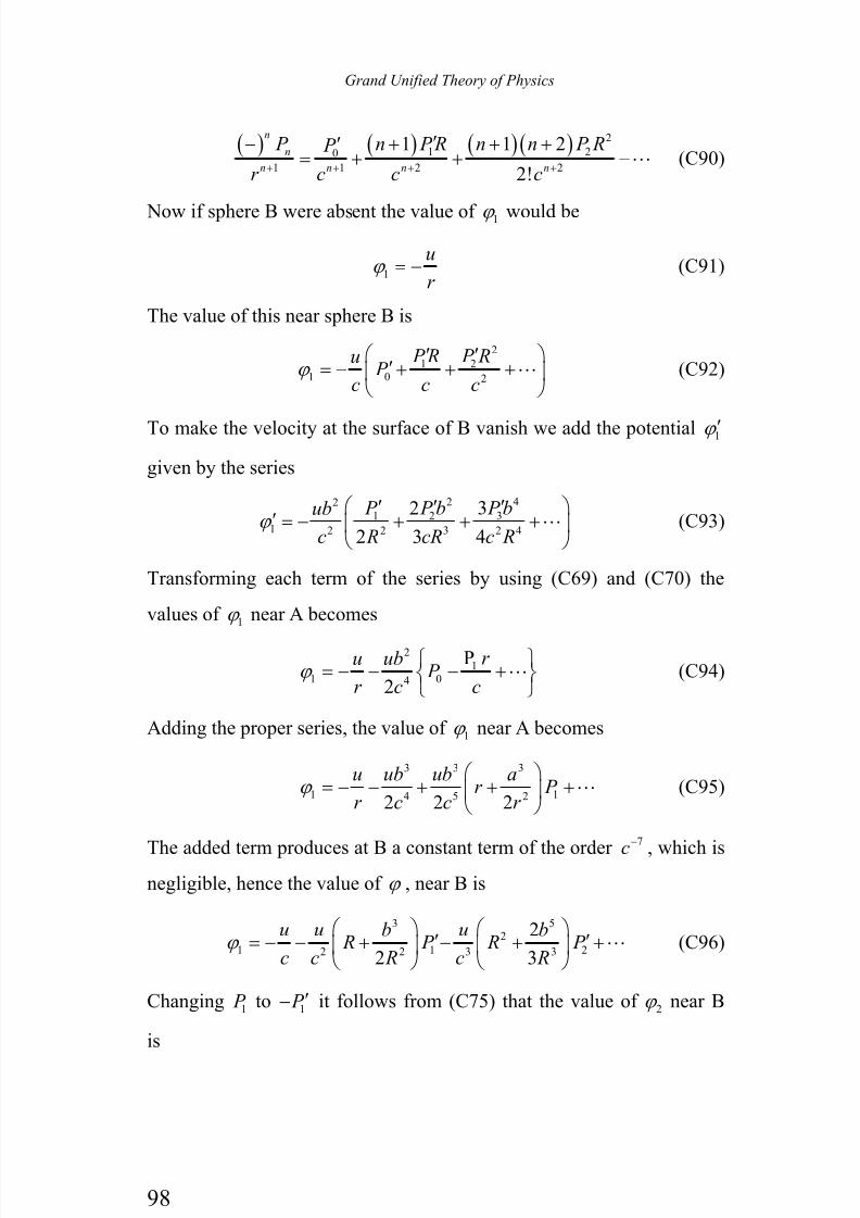
7/30/2019 The Grand Unified-mobilecrackers
http://slidepdf.com/reader/full/the-grand-unified-mobilecrackers 104/143
Grand Unified Theory of Physics
98
( ) ( ) ( ) ( )1 20
1 1 2 2
1 1 2
2!
n
n
n n n n
P n PR n n P R P
r c c c
2
+ + + +
′− + + +′= + + − (C90)
Now if sphere B were absent the value of 1ϕ would be
1
u
r ϕ = − (C91)
The value of this near sphere B is
1 21 0
PR P Ru P
c c cϕ
2
2
′ ′⎛ ⎞′= − + + +⎜ ⎟
⎝ ⎠ (C92)
To make the velocity at the surface of B vanish we add the potential 1ϕ ′
given by the series
31 21 3 4
32
2 3 4
P b P P bub
c R cR c Rϕ
422
2 2 2
′′ ′⎛ ⎞′ = − + + +⎜ ⎟
⎝ ⎠ (C93)
Transforming each term of the series by using (C69) and (C70) the
values of 1ϕ near A becomes
11 0
P
2
r u ub P
r ccϕ
2
4
⎧ ⎫= − − − +⎨ ⎬
⎩ ⎭ (C94)
Adding the proper series, the value of 1ϕ near A becomes
3
1 12 2 2
u ub ub ar P
r c c r ϕ
3 3
4 5 2
⎛ ⎞= − − + + +⎜ ⎟
⎝ ⎠ (C95)
The added term produces at B a constant term of the order 7
c−
, which isnegligible, hence the value of ϕ , near B is
3 5
1 1 2
2
2 3
u u b u b R P R P
c c R c Rϕ 2
2 2 3 3
⎛ ⎞ ⎛ ⎞′ ′= − − + − + +⎜ ⎟ ⎜ ⎟
⎝ ⎠ ⎝ ⎠ (C96)
Changing 1 P to 1 P ′− it follows from (C75) that the value of 2ϕ near B
is
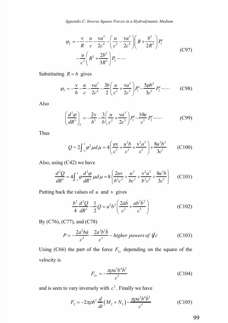
7/30/2019 The Grand Unified-mobilecrackers
http://slidepdf.com/reader/full/the-grand-unified-mobilecrackers 105/143
Appendix C. Inverse Square Forces in a Hydrodynamic Medium
99
3 3 3
2 14 5
5
2
v v v
2 2 2
23
u a u a b R P
R c c c c R
u b R P c R
ϕ 2 2
23 3
⎛ ⎞⎛ ⎞′= − − − − − +⎜ ⎟⎜ ⎟
⎝ ⎠⎝ ⎠
⎛ ⎞− + −⎜ ⎟⎝ ⎠
(C97)
Substituting R b= gives
3 3
2 1 24 5 3
v v 3 v 5
22 2 3
u a b u a b P P
b c c c c c
ϕ ϕ
2
2
⎛ ⎞′ ′= − − − − + − −⎜ ⎟
⎝ ⎠ (C98)
Also
3 3
1 23 3 5 3
2v 3 v 10
2b
d u a u P P
bdR b c c c
ϕ 2
⎛ ⎞ ⎛ ⎞ ′ ′= − − + − −⎜ ⎟ ⎜ ⎟⎝ ⎠ ⎝ ⎠
(C99)
Thus
31
3 5 51
v v 82 4
3
u u b a u bQ d
c c c cϕ µ µ
2 2 2 22
2−
⎛ ⎞= = + + +⎜ ⎟
⎝ ⎠∫ (C100)
Also, using (C42) we have
31
3 5 51
2 v v 84 8
3
d Q d u u a u bd
dR dR b c bc b c c
ϕ ϕ µ µ
2 2 2 2 2
2 2 2 2 2−
⎧ ⎫= = + + +⎨ ⎬
⎩ ⎭∫ (C101)
Putting back the values of u and v gives
5
1 2
4 2
b d Q ab ab bQ a b
dR c c
2 2 2 22 2
2 2
⎛ ⎞− = +⎜ ⎟
⎝ ⎠
(C102)
By (C76), (C77), and (C78)
32 21
a ba a b b P higher powers of c
c c
2 3
2 5= − − −
(C103)
Using (C66) the part of the force 2v F depending on the square of the
velocity is
4
2v
a b b F
c
πρ 3 2
5= −
(C104)
and is seen to vary inversely with 5c . Finally we have
( )3 4 2
2 2 2 52
d a b b F b M N
dt c
πρ πρ 2= − + −
(C105)

7/30/2019 The Grand Unified-mobilecrackers
http://slidepdf.com/reader/full/the-grand-unified-mobilecrackers 106/143
Grand Unified Theory of Physics
100
The value of 1 F , the force on A towards B, is obtained by symmetrically
interchanging “a” and “b”.
Neglecting all powers of 1 c above the second we have
( )2
2 2
2 b d F a ba
dt c
πρ 2= − (C106)
Letting
( )
2sin
2
sin
t a a
T
b b t T
π α
π
β ε
= +
= + −
(C107)
where a and b are the mean radii of the spheres α and β are the
(half) amplitudes of the oscillations, T is the period the oscillation and
ε is the angle the oscillation of B lags A, then the average values of 2 F ,
i.e.,2 F is
( )
( ) ( )
20 0
3
0
3
2 4
16 2 2cos cos
8 2cos
T T
T
d F b a ab dt a b abdt dt Tc Tc
t ab t dt
T T Tc
a b F
T Tc
πρ πρ
π ρ π π αβ ε
π ρ αβ πε
2 2 2 22 2
2
2
2 2
2
= − =
= −
= =
∫ ∫
∫
(C108)
If the spheres are breathing out then in at the same time, that is
if they are in phase ( )0ε = then the force is a maximum value and it is
a force of attraction. When 180° out-of-phase the force is a maximum
and it is a force of repulsion. If the phase differs less than a quarter of a
period they attract each other. If the phase differs more than a quarter
and less than three quarters of a period they will repel each other.
The maximum force between two identical spheres of radius
" "a and vibratory half amplitude " "α is4
max
8 a F
Tc
πρ α 2
2= (C109)
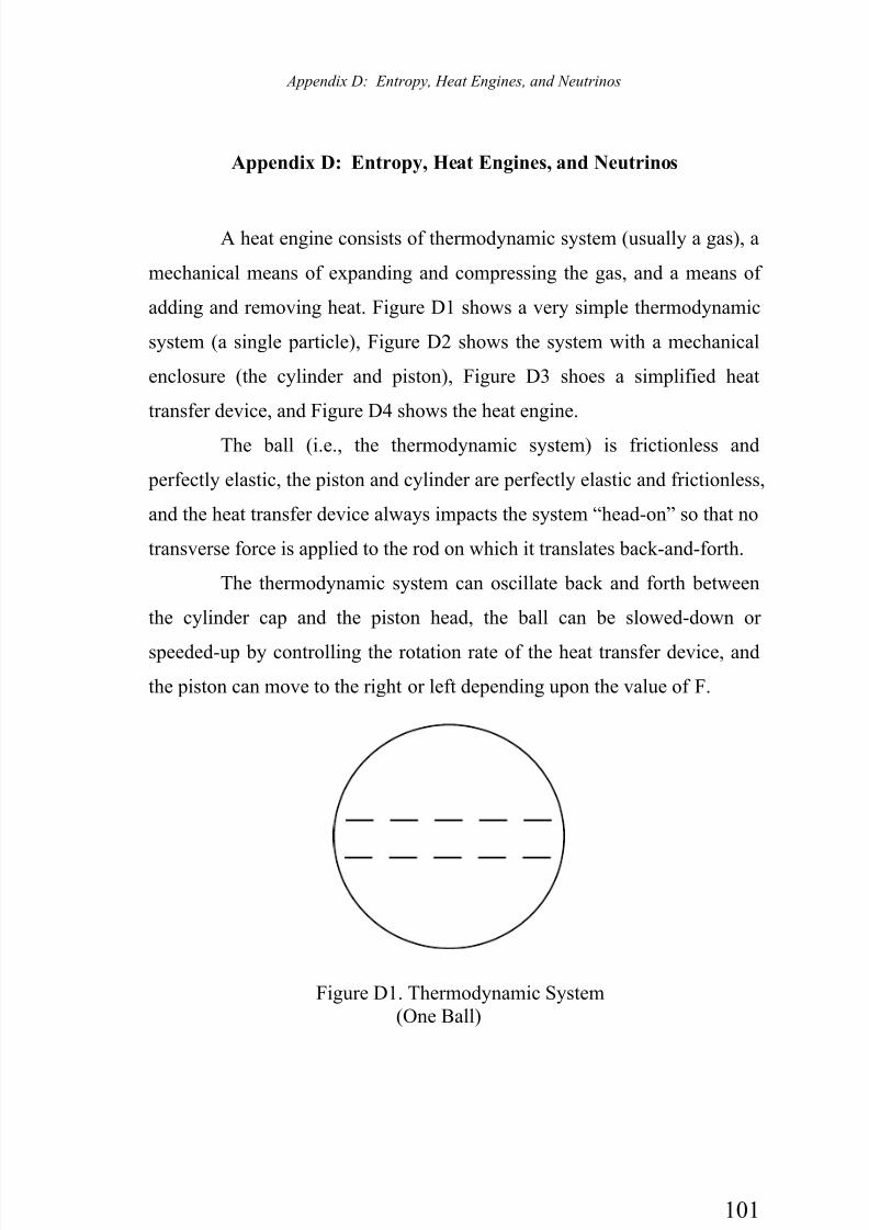
7/30/2019 The Grand Unified-mobilecrackers
http://slidepdf.com/reader/full/the-grand-unified-mobilecrackers 107/143
Appendix D: Entropy, Heat Engines, and Neutrinos
101
Appendix D: Entropy, Heat Engines, and Neutrinos
A heat engine consists of thermodynamic system (usually a gas), a
mechanical means of expanding and compressing the gas, and a means of
adding and removing heat. Figure D1 shows a very simple thermodynamic
system (a single particle), Figure D2 shows the system with a mechanical
enclosure (the cylinder and piston), Figure D3 shoes a simplified heat
transfer device, and Figure D4 shows the heat engine.
The ball (i.e., the thermodynamic system) is frictionless and
perfectly elastic, the piston and cylinder are perfectly elastic and frictionless,
and the heat transfer device always impacts the system “head-on” so that no
transverse force is applied to the rod on which it translates back-and-forth.
The thermodynamic system can oscillate back and forth between
the cylinder cap and the piston head, the ball can be slowed-down or
speeded-up by controlling the rotation rate of the heat transfer device, and
the piston can move to the right or left depending upon the value of F.
Figure D1. Thermodynamic System(One Ball)
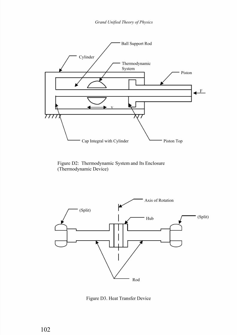
7/30/2019 The Grand Unified-mobilecrackers
http://slidepdf.com/reader/full/the-grand-unified-mobilecrackers 108/143
Grand Unified Theory of Physics
102
Cylinder
Ball Support Rod
Thermodynamic
SystemPiston
F
Cap Integral with Cylinder Piston Top
v
Figure D2: Thermodynamic System and Its Enclosure
(Thermodynamic Device)
Rod
(Split)
Axis of Rotation
Hub (Split)
Figure D3. Heat Transfer Device
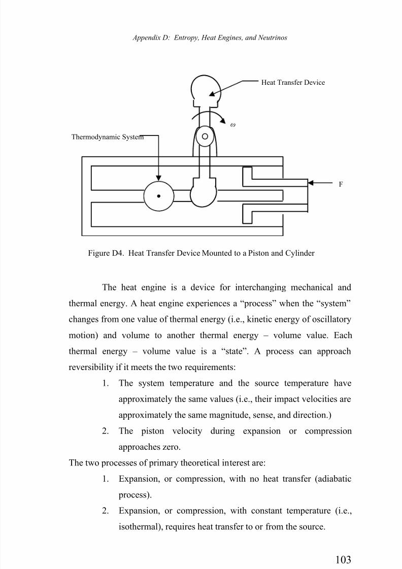
7/30/2019 The Grand Unified-mobilecrackers
http://slidepdf.com/reader/full/the-grand-unified-mobilecrackers 109/143
Appendix D: Entropy, Heat Engines, and Neutrinos
103
The heat engine is a device for interchanging mechanical and
thermal energy. A heat engine experiences a “process” when the “system”
changes from one value of thermal energy (i.e., kinetic energy of oscillatory
motion) and volume to another thermal energy – volume value. Each
thermal energy – volume value is a “state”. A process can approach
reversibility if it meets the two requirements:
1. The system temperature and the source temperature have
approximately the same values (i.e., their impact velocities are
approximately the same magnitude, sense, and direction.)
2. The piston velocity during expansion or compression
approaches zero.
The two processes of primary theoretical interest are:
1. Expansion, or compression, with no heat transfer (adiabatic
process).2. Expansion, or compression, with constant temperature (i.e.,
isothermal), requires heat transfer to or from the source.
Heat Transfer Device
Thermodynamic System
F
ω
Figure D4. Heat Transfer Device Mounted to a Piston and Cylinder
7/30/2019 The Grand Unified-mobilecrackers
http://slidepdf.com/reader/full/the-grand-unified-mobilecrackers 110/143
Grand Unified Theory of Physics
104
Instead of the “one-ball” thermodynamic system let us consider a
gas of many hard, elastic, smooth particles, the “perfect” gas.
In an expansion process in order to approach reversibility thesource temperature (which we always take as a constant value) is slightly
larger than the system temperature and the piston moves very slowly. The
two causes of irreversibility for a thermodynamic system, considered by
thermodynamicists, are:
1. Finite temperature difference between the source and the
thermodynamic system (the gas) and
2. Finite expansion (or compression) speed of the piston.
To understand reversibility and irreversibility we can consider an expansion
followed by a compression. We will consider the expansion as being made
up of two processes. The main reason for using two processes in the
analysis of heat engines is that we have a heat source which remains at
constant temperature and it supplies heat to the engine as the piston expands
and the most work can be done if the heat source and the system are
approximately at the same temperature. This process is followed by an
adiabatic process in order to decrease the system temperature. On the return
compression a constant temperature process permits heat to be dumped
from the gas (which is colder than it was during the isothermal expansion)
to the heat sink. This is followed by an adiabatic compression to return to
the initial condition, if all the processes were reversible. Returning to the
original condition completes one “cycle” of the heat engine.
First we expand using a constant temperature process and we
follow this with a no-heat transfer to or from the system, which is an
adiabatic expansion. (Again, we emphasize that the system is the gas.) In
designing a heat engine the piston stroke is quite constrained and often
specified. Now, by having the two processes any end-point conditions can be obtained between the complete isothermal expansion and the complete
adiabatic expansion by combining the processes differently. Figure D5
shows the pressure, p, versus the specific volume, v, for the two different

7/30/2019 The Grand Unified-mobilecrackers
http://slidepdf.com/reader/full/the-grand-unified-mobilecrackers 111/143
Appendix D: Entropy, Heat Engines, and Neutrinos
105
processes. Now by using a long isothermal expansion followed by a short
adiabatic expansion an end-point pressure just below 2i p will be reached.
Alternatively, if a short isothermal stroke is followed by a long adiabatic
stroke an end-point just above 2a p will be reached.
Let us now obtain the equations for describing the isothermal
expansion and the adiabatic (no-heat-transfer) expansion process. First, we
need an “equation of state”. The equation of state for the ideal gas is simply
the pressure, p, density, ρ , thermal velocity, vr , relation
21v
3r
p ρ = (D1)
This can be written in terms of temperature as follows
2 2 21 1 2 1
v v v3 3 3 2r r r
Nm N
p mV V ρ
⎛ ⎞
= = = ⎜ ⎟⎝ ⎠ (D2)
where N is the total number of particles (all assumed to be alike with mass,
m, and contained in volume V ). Define the temperature T and a constant K
isothermal
adiabatic
p1
p
v1 v v2
p2i
p2a
Figure D5. Isothermal and Adiabatic Expansions
7/30/2019 The Grand Unified-mobilecrackers
http://slidepdf.com/reader/full/the-grand-unified-mobilecrackers 112/143
Grand Unified Theory of Physics
106
such that T is the temperature in degrees Kelvin and K such that KT is the
kinetic energy of one molecule in joules. ( K is the energy in joules of a
particle per degree Kelvin.) Now, define k as( )2 3k K = (D3)
where k is the Boltzmann gas constant, 231.3803 10−× . We now can write
(D2) as
( )2 1 22
3 2 3vr pV N m NKT = =
The number of particles N is the number of moles n of the gas (in the
volume V ) times Avagadros number ( )266.0251 10o N = × particles per
kilogram mole. Now we have
( ) ( ) ( )0 0 02 3 2 3 pV nN KT n N K T nN k T = = =⎡ ⎤⎣ ⎦ (D4)
Most physicists and chemists define the gas constant pc R as
pc o R kN = (D5)
so that the gas equation of state is
v pc p nR T = (D6)
Engineers generally define the gas constant e R as
e pc R nR= (D7)
so that the gas equation is
e PV MR T = (D8)
We will use (D8) except that we generally divide both sides of the equation
by M and use the specific volume v which is
V v = (D9)
then
e pv R T = (D10)
7/30/2019 The Grand Unified-mobilecrackers
http://slidepdf.com/reader/full/the-grand-unified-mobilecrackers 113/143
Appendix D: Entropy, Heat Engines, and Neutrinos
107
For the isothermal reversible process going from state 1 to state 2
with so g T T = where soT is the source absolute temperature and g T is the
gas temperature, the energy balance is
1 2wq →= (D11)
since the internal energy is constant. In this expression 1,2q is the heat
transferred per unit mass of the gas and 1 2w → is the work done by the gas
going from state 1 to state 2. The work is given by
22
1 2 11
2
1w v lne
e
R T v
pdv d R T v v→ = = =∫ ∫(D12)
Consider now the adiabatic reversible process from state 2 to state 3. The
energy balance is
( )2 3 wq q du d δ → = = +∫ ∫ (D13)
Now 0qδ = and
wd pdv= (D14)
so
du pdv= − (D15)
Further, the specific heat at constant volume " "v
c is given by
v
duc
dT = (D16)
Where u is the internal energy of the gas. Thus
vdu c dT pdv= = − (D17)
The energy balance can be written in terms of the enthalpy h where
h u pv= + (D18)
and
dh du pdv vdp= + + (D19)
or
du pdv dh vdp+ = − (D20)

7/30/2019 The Grand Unified-mobilecrackers
http://slidepdf.com/reader/full/the-grand-unified-mobilecrackers 114/143
Grand Unified Theory of Physics
108
Thus
q du pdv dh vdpδ = + = − (D21)
The specific heat at constant pressure " " pc is given by
p
dhc
dT = (D22)
or
pdh c dT = (D23)
Now, using (D21) and (D23) with 0qδ = we obtain
pc dT vdp= (D24)
Dividing (D24) by (D16)
p
v
c dT vdp
c dT pdv= − (D25)
Using
p
v
c
k c= (D26)
gives
v dpk
p dv= − (D27)
Integrating from state 2 to state 3 gives
3 33 3 2
2 22 2 3
ln ln ln
k
v v pdv dpk k
v p v v p
⎛ ⎞= − = = =⎜ ⎟
⎝ ⎠∫ ∫ (D28)
Now, we have
2 2 3 3
k k k p v p v pv c= = = (D29)
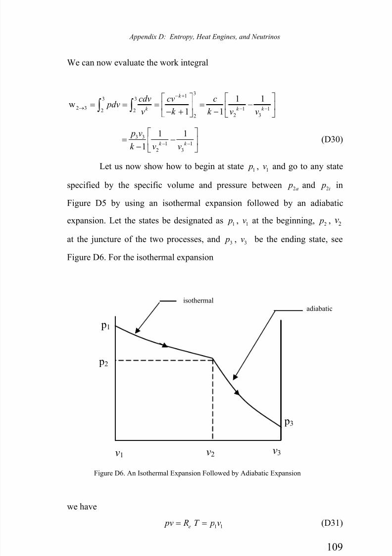
7/30/2019 The Grand Unified-mobilecrackers
http://slidepdf.com/reader/full/the-grand-unified-mobilecrackers 115/143
Appendix D: Entropy, Heat Engines, and Neutrinos
109
We can now evaluate the work integral
313 3
2 3 1 12 22 32
1 1w1 1
k
k k k
cdv cv c pdvk k v v v
− +
→ − −⎡ ⎤⎡ ⎤= = = = −⎢ ⎥⎢ ⎥
− + −⎣ ⎦ ⎣ ⎦∫ ∫
3 3
1 1
2 3
1 1
1 k k
p v
k v v− −
⎡ ⎤= −⎢ ⎥
− ⎣ ⎦(D30)
Let us now show how to begin at state 1 p , 1v and go to any state
specified by the specific volume and pressure between 2a p and 2i
p in
Figure D5 by using an isothermal expansion followed by an adiabatic
expansion. Let the states be designated as 1 p , 1v at the beginning, 2 p , 2v
at the juncture of the two processes, and 3 p , 3v be the ending state, see
Figure D6. For the isothermal expansion
we have
1 1e pv R T p v= = (D31)
isothermaladiabatic
p1
p2
v1 v2 v3
p3
Figure D6. An Isothermal Expansion Followed by Adiabatic Expansion

7/30/2019 The Grand Unified-mobilecrackers
http://slidepdf.com/reader/full/the-grand-unified-mobilecrackers 116/143
Grand Unified Theory of Physics
110
and for the adiabatic expansion we have
3 3
k k pv p v= (D32)
At the juncture we equate the pressures and the specific volumes. From
(D31)
2 1 1 2 p p v v= (D33)
Substituting into (D32) we have
1 12 3 3
2
k k p vv p v
v
= (D34)
or
1
113 3
2 1
1 11
k
k k
k
p vv
pv
−−
−
⎛ ⎞= ⎜ ⎟
⎝ ⎠(D35)
and
1 1 1
1 1 1 1 1 11 1 1 1 1 1 1 1
2 11 1
3 31 1 1 13 1 3 3
k k k
k k k k k k
k k
k k k k
p v p v p v p v p p
p v p v p v
− − − − − −
− − − −
⎛ ⎞ ⎛ ⎞= = = ⎜ ⎟ ⎜ ⎟
⎝ ⎠ ⎝ ⎠(D36)
Now
2 22
1,2 1,2 1 21 1
1
w 0 lne e
vdvq pdv R T R T
v vµ →∆= + = + = =∫ ∫ (D37)
In terms of 1 p , 1v , 3 p , 3v we have
1
1 13 3 3 3
1,2
1 1 1 1
1ln ln ln
1 1
k
k k
e e
p v p vk q R T R T
p v k p k v
− −⎡ ⎤⎛ ⎞ ⎛ ⎞ ⎡ ⎤⎢ ⎥= = +⎜ ⎟ ⎜ ⎟ ⎢ ⎥⎢ ⎥ − −⎝ ⎠ ⎝ ⎠ ⎣ ⎦⎢ ⎥⎣ ⎦
(D38)
Using
p v ec c R− = (D39)
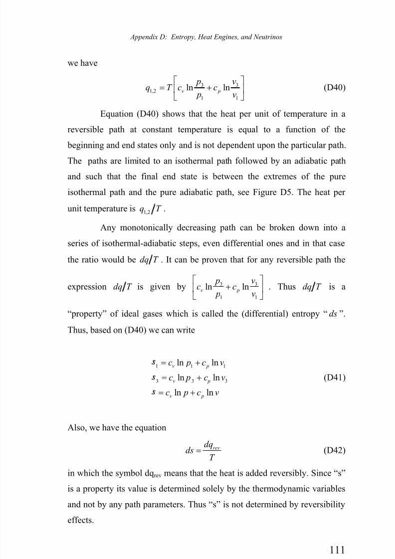
7/30/2019 The Grand Unified-mobilecrackers
http://slidepdf.com/reader/full/the-grand-unified-mobilecrackers 117/143
Appendix D: Entropy, Heat Engines, and Neutrinos
111
we have
3 31,2
1 1
ln lnv p
p vq T c c
p v
⎡ ⎤= +⎢ ⎥
⎣ ⎦
(D40)
Equation (D40) shows that the heat per unit of temperature in a
reversible path at constant temperature is equal to a function of the
beginning and end states only and is not dependent upon the particular path.
The paths are limited to an isothermal path followed by an adiabatic path
and such that the final end state is between the extremes of the pure
isothermal path and the pure adiabatic path, see Figure D5. The heat per unit temperature is 1,2
q T .
Any monotonically decreasing path can be broken down into a
series of isothermal-adiabatic steps, even differential ones and in that case
the ratio would be dq T . It can be proven that for any reversible path the
expression dq T is given by 3 3
1 1
ln lnv p
p vc c
p v
⎡ ⎤+⎢ ⎥
⎣ ⎦
. Thus dq T is a
“property” of ideal gases which is called the (differential) entropy “ ds ”.
Thus, based on (D40) we can write
1 1 1
3 3 3
ln ln
ln ln
ln ln
v p
v p
v p
c p c v
c p c v
c p c v
= +
= +
= +
(D41)
Also, we have the equation
revdq
dsT
= (D42)
in which the symbol dqrev means that the heat is added reversibly. Since “s”
is a property its value is determined solely by the thermodynamic variables
and not by any path parameters. Thus “s” is not determined by reversibility
effects.
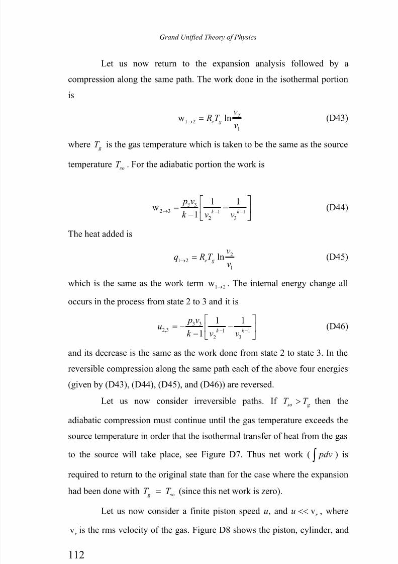
7/30/2019 The Grand Unified-mobilecrackers
http://slidepdf.com/reader/full/the-grand-unified-mobilecrackers 118/143
Grand Unified Theory of Physics
112
Let us now return to the expansion analysis followed by a
compression along the same path. The work done in the isothermal portion
is
21 2
1
w lne g
v R T
v→ = (D43)
where g T is the gas temperature which is taken to be the same as the source
temperature so
T . For the adiabatic portion the work is
3 32 3 1 1
2 3
1 1w
1 k k
p v
k v v→ − −
⎡ ⎤= −⎢ ⎥− ⎣ ⎦
(D44)
The heat added is
21 2
1
lne g
vq R T
v→ = (D45)
which is the same as the work term 1 2w → . The internal energy change all
occurs in the process from state 2 to 3 and it is
3 32,3 1 1
2 3
1 1
1 k k
p vu
k v v− −
⎡ ⎤= − −⎢ ⎥
− ⎣ ⎦(D46)
and its decrease is the same as the work done from state 2 to state 3. In the
reversible compression along the same path each of the above four energies
(given by (D43), (D44), (D45), and (D46)) are reversed.
Let us now consider irreversible paths. If so g
T T > then the
adiabatic compression must continue until the gas temperature exceeds the
source temperature in order that the isothermal transfer of heat from the gas
to the source will take place, see Figure D7. Thus net work ( pdv∫ ) is
required to return to the original state than for the case where the expansion
had been done with g soT T = (since this net work is zero).
Let us now consider a finite piston speed u, and vr u << , where
vr is the rms velocity of the gas. Figure D8 shows the piston, cylinder, and
7/30/2019 The Grand Unified-mobilecrackers
http://slidepdf.com/reader/full/the-grand-unified-mobilecrackers 119/143
Appendix D: Entropy, Heat Engines, and Neutrinos
113
gas. The internal energy of the gas per unit mass is ( ) 21 2 vrso ρ , where vrso
is the rms velocity of the gas when initially at the source temperature. When
the piston moves at velocity u the average flow velocity of the gas is
2u and its flow energy is ( ) 21 8 u ρ .
Gasvr =
rms velocity
Cylinder
Piston
u
Figure D8. Piston Moving at Velocity u.
F
IsothermalCompression
at Tso
Adiabatic
Expansion
p1
v1 v2 v3
p3
Figure D7. Expansion followed by Compression when Tso > Tg
2
p1'
Isothermal Expansion
Tg < Tso
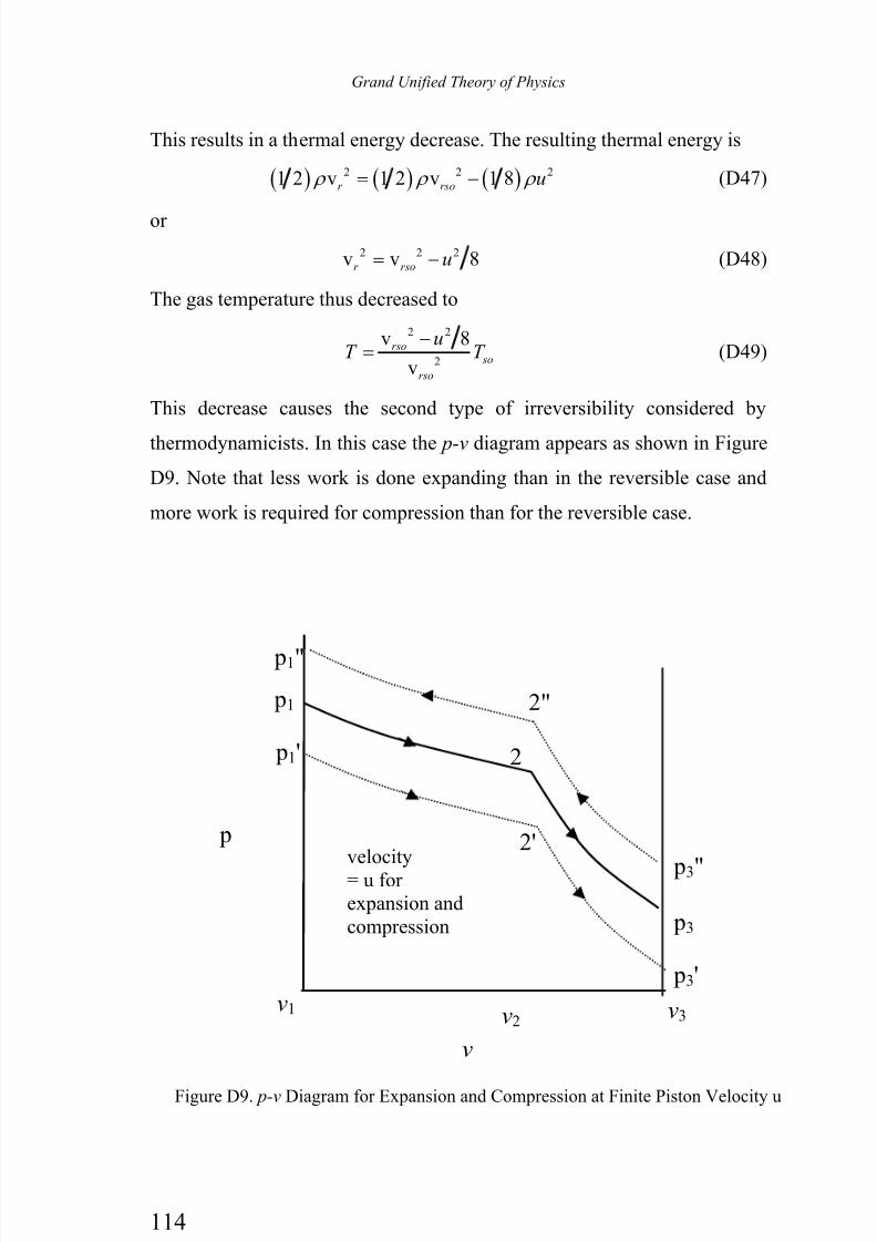
7/30/2019 The Grand Unified-mobilecrackers
http://slidepdf.com/reader/full/the-grand-unified-mobilecrackers 120/143
Grand Unified Theory of Physics
114
This results in a thermal energy decrease. The resulting thermal energy is
( ) ( ) ( )2 2 21 2 v 1 2 v 1 8r rso u ρ ρ ρ = − (D47)
or
2 2 2v v 8r rso u= − (D48)
The gas temperature thus decreased to
2 2
2
v 8
v
rso
so
rso
uT T
−= (D49)
This decrease causes the second type of irreversibility considered by
thermodynamicists. In this case the p-v diagram appears as shown in Figure
D9. Note that less work is done expanding than in the reversible case and
more work is required for compression than for the reversible case.
p1
v1 v2v3
p3
Figure D9. p-v Diagram for Expansion and Compression at Finite Piston Velocity u
2"
2'
p1"
p3'
p3"
p1'
p
v
2
velocity= u for expansion andcompression
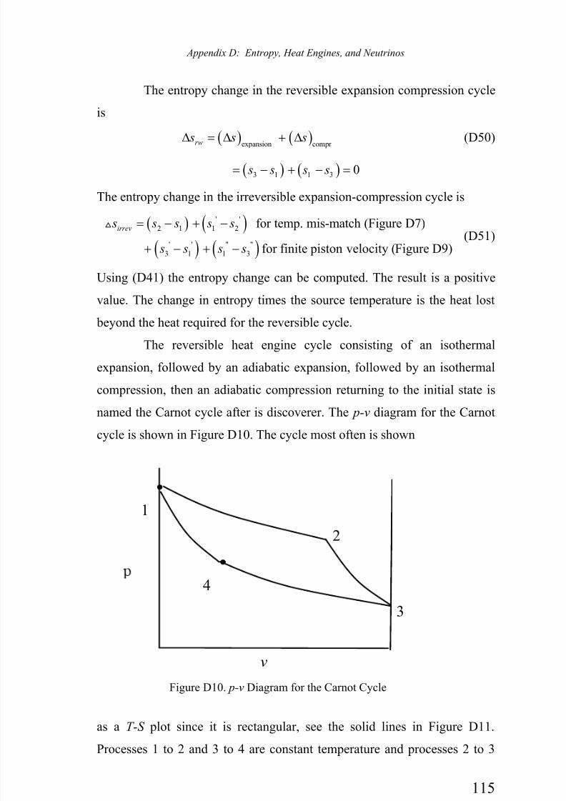
7/30/2019 The Grand Unified-mobilecrackers
http://slidepdf.com/reader/full/the-grand-unified-mobilecrackers 121/143
Appendix D: Entropy, Heat Engines, and Neutrinos
115
The entropy change in the reversible expansion compression cycle
is
( ) ( )expansion compr rw s s s∆ = ∆ + ∆ (D50)
( ) ( )3 1 1 3 0 s s s s= − + − =
The entropy change in the irreversible expansion-compression cycle is
( ) ( )
( ) ( )
' '
2 1 1 2
' ' " "
3 1 1 3
for temp. mis-match (Figure D7)
for finite piston velocity (Figure D9)
irrev s s s s s
s s s s
= − + −
+ − + −
(D51)
Using (D41) the entropy change can be computed. The result is a positivevalue. The change in entropy times the source temperature is the heat lost
beyond the heat required for the reversible cycle.
The reversible heat engine cycle consisting of an isothermal
expansion, followed by an adiabatic expansion, followed by an isothermal
compression, then an adiabatic compression returning to the initial state is
named the Carnot cycle after is discoverer. The p-v diagram for the Carnot
cycle is shown in Figure D10. The cycle most often is shown
as a T-S plot since it is rectangular, see the solid lines in Figure D11.
Processes 1 to 2 and 3 to 4 are constant temperature and processes 2 to 3
v
Figure D10. p-v Diagram for the Carnot Cycle
4
1
3
2

7/30/2019 The Grand Unified-mobilecrackers
http://slidepdf.com/reader/full/the-grand-unified-mobilecrackers 122/143
Grand Unified Theory of Physics
116
and 4 to 1 are constant entropy (since dq Tds= , and dq is zero). The
temperature T si is
the “cold” sink to which heat is dumped on the compression cycle. An
irreversible cycle is shown by the dotted lines in Figure D11.
In all macroscopic cycles the entropy is universally observed to
increase. Entropy forms the basis for design decisions in all thermal systems
and in the analysis of biological processes. Microscopic cycles, such as
molecular orbits, however have neither entropy increases nor decreases.
The theory of physics here rests upon the assumed stability of the
neutrino. The entropy for a cycle of its action is computed by determining
the entropy of the ambient “gas” which is ready to flow into the neutrino
then compute the entropy of that same “gas”, which by then has changed to
a solid, as it exits from the neutrino. The entering entropy is
1 2
4 3
0T
Si
Figure D11. T-S Diagram for the Carnot Cycle
Tsi
Tso
S0
2'
3'4'
S
1'
7/30/2019 The Grand Unified-mobilecrackers
http://slidepdf.com/reader/full/the-grand-unified-mobilecrackers 123/143
Appendix D: Entropy, Heat Engines, and Neutrinos
117
1 1 1ln lnv pc p c v= + (D52)
The exiting entropy is
2 2 2ln lnv pc p c v= + (D53)
At the exit the pressure is zero, since the particles are all aligned. Further,
the specific volume (volume per unit mass) is essentially zero. Thus, 2 0 s ≈
and 2 1 s− is negative. Thus the neutrino, as it is envisioned here, is an
entropy reducer.
Contemporary physics rejects the possibility that such a state as
envisioned for the neutrino is possible. However, the arguments presented
in this book make the neutrino state seem plausible, but certainly do not
prove it is possible. On the other hand contemporary physics assumes that
all the organization was placed in a minute ball which has been expanding
for ten billion years and provides the organization observed as it is
expanding. When the kinetic particle theory of physics is judged against the
expanding ball the kinetic particle theory sounds better!!

7/30/2019 The Grand Unified-mobilecrackers
http://slidepdf.com/reader/full/the-grand-unified-mobilecrackers 124/143
Grand Unified Theory of Physics
118
Appendix E: A Personal History of the Kinetic Particle Unified Physics
Many of my fellow members of the American Physical Society
will look at this book, possibly glance at the simple set of postulates, then
immediately dismiss the book. They would immediately think it impossible
to derive all the complexities of physics starting with just one “billiard ball”
type of particle. Recently I prepared a paper, which essentially was the
contents of this book, and submitted it to several physics journals for their
review. I feel safe in saying that none of the reviewers read the paper
carefully enough to understand its content.
Such a reception of a new structure of physical science, even when
it better explains the way the universe works, is normal. Thomas Kuhn in
his book The Structure of Scientific Revolution [21] calls a new
comprehensive theory a paradigm. In his book he explores several different
paradigms throughout the history of science. The general pattern is that theold scientists cling to their paradigm until they die and the following
generation adopts the new theory.
This may be my last writing in physics, I was 76 years old on
January 9, 2004, so I thought it worthwhile to document what I remember 1
about the development of this theory. I will first start by giving some of my
background before starting to work on the theory.
I was born in the rural community of Gatewood near Fayetteville,
West Virginia. My parents were Paul Alexander Brown and Mary Lou Fox
Brown. I have an older brother Paul Jerry Brown born July 28, 1925
1 I could write a book entitled What Little I Remember like Frisch [24]wrote. However, my book probably would be much shorter than his.
7/30/2019 The Grand Unified-mobilecrackers
http://slidepdf.com/reader/full/the-grand-unified-mobilecrackers 125/143
Grand Unified Theory of Physics
119
and a younger sister Mary Jane Brown Songer, born November 13, 1929.
We lived on a 10 acre plot and had a garden, chickens, and a milk cow. My
father worked in the coal mines during the evenings and repairedautomobiles and built houses during the days. We went to the Church of the
Brethren nearly every Sunday. We were very poor during the depression
years, 1930 to 1940.
We ran throughout the neighborhood and played most of these
depression years. We spent a lot of time running at full speed playing fox
and hounds. The West Virginia hills were beautiful in the summer, and in
the winter, as well as in the spring and fall. One of our best toys often was a
pot lid which we used as our automobile (actually just the steering wheel).
There was a story of a boy who lived in the town of Fayetteville 3 miles
away who “drove” his lid car to our school every morning for one whole
school year. Turned around by backing his car down the lane beside our
school, and of course looking over his right shoulder as he was shifting into
reverse steering his car and backing down, stopping, then shifting into first
gear and driving back to Fayetteville.
I attended Victory Grade School, a 3 room 3 classes per room
facility, until graduation in 1940. I read all the books I could find, which
were about 4 or 5 school books a year. I then attended Fayetteville High
School, graduating at 15 years of age in 1943. Throughout the first 13
grades of school I excelled in grammar, history, and mathematics –
anything where logic and memory were useful.
I studied engineering the next 9 years first at West Virginia Tech,
then West Virginia University (obtaining a BS in 1946 and a BSME in
1947) then at Purdue University (obtaining an MSME degree in 1950,1and a
PhD in 1952).
1 There was a semester interruption of my Purdue stay by a fall 1947semester at Cornell University.
7/30/2019 The Grand Unified-mobilecrackers
http://slidepdf.com/reader/full/the-grand-unified-mobilecrackers 126/143
Grand Unified Theory of Physics
120
I was at West Virginia Tech during wartime and Professor “Daddy
Boy” Smith was the only math teacher. There were 20 math students taking
approximately 10 different courses each semester. There was no way hecould lecture on so many subjects so the first day of class he made certain
we had the correct book. He then told us to work the odd problems and
submit them for credit in the course. He told us to come to his office if we
needed help. I soon found he could not help me and I had to “learn-on-my-
own”. I self-taught five courses including calculus. I was fascinated by the
infinite processes of calculus. To better learn the subject, I re-took calculus
when I transferred to West Virginia University. One highlight at West
Virginia University was the final lecture by Professor Ford in physics. He
explained the quantum levels of atoms – how one electron jumps from one
orbit to another emitting, or absorbing a photon. It was fascinating and
believable.
My graduate courses were equally divided among mathematics,
mechanics, and mechanical design. My background in mechanical design,
engineering mechanics, and the mathematics required for modeling
mechanical systems was the ideal background for developing a mechanical
model of the universe.
During my school years there were several phenomena which
struck me as extremely profound:
1. How does a lightning bug produce light?
• A pre-school/kindergarten question
2. Why do iron filings on a paper above a magnet make their
characteristic patterns?
• A sixth grade demonstration
3. The mathematical modeling the lever and trusses was a fascinating
joining of mathematics and physics.4. I heard something from a fellow student at Cornell University
about Einstein’s mass growth or matter shortening. I was
astounded and unbelieving, but I don’t remember any details.
7/30/2019 The Grand Unified-mobilecrackers
http://slidepdf.com/reader/full/the-grand-unified-mobilecrackers 127/143
Appendix E: A Personal History of the Kinetic Particle Unified Physics
121
5. During my school career (as well as before and even after) I have
often dreamed of personally overcoming gravity. I often stood
unsupported above the ground while people were around – but theynever noticed even when I told them. Also, I could run by taking
long and longer strides, often 100 meter strides.
Soon after leaving Purdue I moved to California and met an American
Airlines stewardess Miss Jimmie Marie Dikeman from Oolagah, Oklahoma.
We were soon married, January 18, 1952, and begat four children, Paul
Alexander Brown II was born January 18, 1953; Stephanie Ann Brown was
born June 27, 1956; Barbara Louise Brown was born October 1, 1959; and
Carolyn Jane Brown was born July 11, 1962.
I spent 19 years in aircraft structural analysis, aerospace design
management, and physics research at various aerospace companies from
1951 through 1970. I started teaching engineering mechanics part-time at
West Virginia University in 1947 and continued at the University of
Southern California, and UCLA. I began teaching design, thermodynamics,
and engineering mechanics full-time at Mississippi State University and
continued for 21 years from 1970 thru 1991. The last 13 years I have spent
approximately half time doing research.
In 1958 while I was a first level manager at Hughes Aircraft Company I
got the idea that gravitation was produced by ether particles in space
somehow pushing bodies together. In 1963 while I was a second level
manager at the Aerospace Corporation in El Segundo, California I stumbled
across the idea that gravitation was caused by a mutual shielding of one
body be another and that the ether particles pushed the bodies together.
(Later I discovered the idea was fallacious. Gravitation is caused by matter
producing a distant expansion-contraction wave in the ether and that lets the
ether push the bodies together.) I worked on the ether particle theory until1967 at the Aerospace Corporation and finally evolved the concept that
everything was made up the same particles that make up the ether. I
published 3 books in this period of time: (References [13], [14], and [15])
7/30/2019 The Grand Unified-mobilecrackers
http://slidepdf.com/reader/full/the-grand-unified-mobilecrackers 128/143
Grand Unified Theory of Physics
122
1. Unified Physics Part 1 JMB Co, Box 45004, Los Angeles, CA 90045,
1965.
2 Advanced Physics, JMB Co, Box 153, Los Angeles, CA 90045, 1966.3. Advanced Physics, 3rd Edition, JMB Co, Box 153, Los Angeles, CA
90045, 1967.
These books had many fundamental errors but I felt they would advance the
development of the kinetic particle theory of physics.
While at the Aerospace Corporation in 1966 I requested support
for my efforts from the president of the corporation, the late Dr. Ivan
Getting. He formed a panel, chaired by Dr. Jack Irving, to review my work.
(The Corporation had recently sent Dr. Irving to the California Institute of
Technology to obtain his PhD.) I made a presentation which I felt all
members of the panel would feel the world surely must be made up of
kinetic particles. They didn’t. As I left the presentation one of the panel
members Dr. Robert Huddelstone remarked that it was unbelievable that I
would sacrifice my career as an engineering manager (I was an associate
department head at the time) on a fantasy. I thought he would soon see I
was on the right track. In the presentation Dr. Irving asked me if I wanted
to study physics at Cal Tech (as I remember). I said, I wanted to continue
working physics part time. In later years I either heard, or deduced, that Dr.
Getting was willing to fund my education to obtain a PhD in physics. If so, I
still would not have accepted the offer primarily because I thought the
physics I would be taught would be incorrect-particularly the relativity
theory.
The third book I had published Advanced Physics – 3rd
Edition
addressed more than physics. It was my first step toward organizing all of
science. Even with its severe limitations it came into the hands of Dr.
Robert M. Wood the deputy director of Research at Douglas AircraftCompany, in Santa Monica, California. It lead me into a job wherein I could
develop my theory of physics, which I so ardently wanted.
7/30/2019 The Grand Unified-mobilecrackers
http://slidepdf.com/reader/full/the-grand-unified-mobilecrackers 129/143
Appendix E: A Personal History of the Kinetic Particle Unified Physics
123
Dr. Wood believed that unidentified flying objects (UFOs) were
spacecraft built and manned by extra-terrestrials. Because of the great
distances to other stars he believed that the vehicles could travel at speedsorders of magnitude greater than the speed of light. Furthermore, he had
great confidence in his ability. “If extraterrestrial’s can build a flying saucer,
so can I.”
Dr. Wood had an associate, Dr. Darell B. Harmon, Jr., Dr. Harmon
was the inventor and subsequent manager of a major project at the Douglas
Aircraft Company to develop “external burning” for greatly enhancing
maneuverability of anti-ballistic missile defense rockets. Dr. Harmon held
beliefs about UFO’s similar to Dr. Wood.
Dr. Wood interviewed me for employment and asked what I
believed regarding a list of some dozen subjects. One of the subjects was
UFOs. My answer was that I believed they were real but natural
atmospheric disturbances. Dr. Wood believed that UFO’s were powered by
anti-gravity propulsion and I was researching gravity so he hired me in spite
of my disbelief in extraterrestrials. Thus the Wood-Harmon-Brown team
was formed to invent a new propulsion system based on obtaining an
understanding of the mechanism of gravity.
Well here we were, our leader Bob Wood, and our consultant
Darell Harmon, both of whom worked full-time at other tasks, and I, who
was promised at least half of my time to work on my theory and the
remainder to work on Bob’s projects, whatever they may be. All three of us
had been very satisfied with our engineering endeavors. All of us had the
best backgrounds possible to develop a mechanical theory of physics. All
three of us rejected the tenets of relativity theory (I thought all the known
relativity experiments could be derived from classical theory and Bob and
Darell thought super-optic travel was possible), and we had the vastresources of Douglas Aircraft Company at our disposal. We were ready to
go. We hired an experienced and well trained mathematical physicist, Dr.
7/30/2019 The Grand Unified-mobilecrackers
http://slidepdf.com/reader/full/the-grand-unified-mobilecrackers 130/143
Grand Unified Theory of Physics
124
Leon A. Steinert just to make sure we had all the tools-of-the-trade at our
disposal.
We were housed in the main building at the Douglas AircraftCompany Santa Monica California plant. Our room was a five meter square
vault which previously had been used for storing secret documents. The
door was steel with a combination lock. In addition to the mathematical
physicist, Leon, we hired an experimentalist Harvey Bjornlie, a retired Los
Angeles, California police detective Paul Wilson, a UFO “buff” Stan
Friedman, and a psychic Chan P. Thomas.
Chan had been instrumental in promoting the project from its
outset. In fact, he is the person who discovered my book Advanced Physics
and had recommended Bob to hire me. Stan was hired because of his wealth
of background on flying saucer sightings. Paul was hired to investigate the
flying saucer reports in depth. Bob essentially ran the flying saucer
investigative effort, Darell was basically in charge of the experimental
efforts, and I was in charge of the theoretical effort. Our budget was less
than $100,000.00 per year. The total expenditure of our project in its three
year existence was probably less than the US Air Force spent on the project
headed by Dr. E.U. Condon [21] trying to prove there were no flying
saucers. Incidentally, in the Condon report the researchers found what they
believed were flying saucers, but Condon’s summary denied their results. In
the following paragraphs I will report only the results of the theoretical
efforts.
My three year tenure at Douglas was like “dying-and-going-to-
heaven”. I almost had all my time free to work on the kinetic particle theory
of physics. Darell and I searched libraries and all the book stores in the Los
Angeles area looking for information useful to the project. I bought and
read every book that could be of interest. (I read 1000 books in the threeyear period.) Leon was an accomplished teacher. He taught me how to use
tensors which are required in the analysis of the flow of kinetic particles.

7/30/2019 The Grand Unified-mobilecrackers
http://slidepdf.com/reader/full/the-grand-unified-mobilecrackers 131/143
Appendix E: A Personal History of the Kinetic Particle Unified Physics
125
I spent approximately a year developing what I called “the
Continuum Equation for Kinetic Particles”. In this equation I assumed for
each small volume of space considered there were enough particles so thatthe continuum assumption on space density and velocity density were valid,
but did not assume the velocities were Maxwell-Boltzmann distributed. I
dropped this effort later when it appeared that the Maxwell-Boltzmann
distribution might be valid.
Bob and I went to a seminar on cosmology at the Douglas
Research Division. There was some of Arthur Eddington’s work discussed
on relating cosmological parameters to macroscopic and even microscopic
parameters. Bob got the idea he could interrelate all these parameters just
using dimensional analysis. He also may have been influenced by the
incredible paper by diBertini [22] in which most of the constants of physics
were interrelated by a stochastic mathematical structure. The fine structure
constant was not mentioned in diBertini’s paper nor in the efforts of Bob’s.
Anyway, Bob and Harvey worked on the dimensional analysis for several
months.
I kept cognizant of Bob and Harvey’s dimensional analysis and by
relating cosmological magnitudes to microscopic magnitudes I related the
basic particle (brutino) mass to the mass of the universe and the brutino
diameter to the radius of the universe. Anyway, I guessed that the brutino
diameter was the Planck length ( )3510 m− and the mass was 6510 kg − ,
something of the order of the graviton energy divided by the square of the
speed of light. This then lead to the idea that the Hubble red shift was due to
the loss of one brutino for each wave length which the photon executes
during its travel through space.
The bulk of my time the next two years was spent on dreaming up
models of the electron, proton, and photon. None of these models withstood
the scrutiny of experiment. The only significant milestone reached was the
discovery that ( )2
v v vr m r −⎡ ⎤⎣ ⎦ was very close to the value of the fine

7/30/2019 The Grand Unified-mobilecrackers
http://slidepdf.com/reader/full/the-grand-unified-mobilecrackers 132/143
Grand Unified Theory of Physics
126
structure constant (one part in 310 ). Since this constant times the speed of
light gives the electron orbital velocity which is controlled by inertia, when
the speed is adjusted by using a center of mass system the agreement is one
part in 510 , as discovered by Darell. Bob, Darell, and I all realized this was
extremely significant and almost assured us that the kinetic particle theory
of physics was valid. We published this result in 1970 [1].
However, hard times came. Douglas Aircraft had been absorbed by
McDonnell Aircraft to form McDonnell Douglas Corp in 1967, shortly after
my employment. In 1970, the Air Force cancelled the McDonnell DouglasMOL (Manned Orbiting Laboratory) Project. Funds began to be scarce.
McDonnell Douglas had retained Dr. Richard P. Feynman as a
consultant and Dr. Feynman was requested to review our project (actually,
just the theoretical physics portion). Bob and Darell went to the review.
Even in spite of Darell’s vehement objections at the meeting, the project
was cancelled. Dr. Feynman saw no merit in the work. He ignored the
significance of the factor ( )2
v v vr m r −⎡ ⎤⎣ ⎦ being close to the fine structure
constant. Further, he said the center-of-mass correction was not valid.
Surely Dr. Feynman knew that this correction was valid. Even further, in his
book QED which he published some 15 years later, he discusses the fine
structure constant, see Feynman [7], on pages 129 and 130. He referenced
Arthur Eddington’s numerology giving the value 136 for 1 α but he never
mentioned our raw value of 137.1087 nor our corrected value of 137.0341
versus the measured value of 137.0360. It appeared that Dr. Feynman felt
that we should not be encouraged without first obtaining a proper physics
background. In fact, he once told me to “Come up through the ranks.”1 In
any case the project was cancelled.
Thus, as a result of three years research we had discovered thenumerical connection between the fine structure constant and the kinetic
1Many years later I thought that might have been an easier route than what I had taken.
7/30/2019 The Grand Unified-mobilecrackers
http://slidepdf.com/reader/full/the-grand-unified-mobilecrackers 133/143
Appendix E: A Personal History of the Kinetic Particle Unified Physics
127
particle ether. (We were not able to discover the mechanism connecting the
two until some 30 more years passed.) Also, we knew the mechanism of the
Hubble red shift and the mass of the basic particle i.e., the brutino). We hadguessed at the particle diameter but had no mechanism for computing its
diameter.
I decided to seek a university setting for the continuation of my
physics research. I wanted to locate a university in a rural setting where I
could teach engineering and work on the kinetic particle theory. I wanted to
teach engineering, since I had done that a lot over almost a quarter century
prior to the project cancellation. I felt engineering teaching would be
intellectually soothing since the kinetic particle research had become
stressful.
I located the ideal job as a professor of mechanical engineering at
Mississippi State University (MSU). Dr. C.T. Carley employed me to teach
mechanical engineering design and to develop research in the department.
MSU was a university with 8000 students and it was adjacent to Starkville
Mississippi, a town of 16,000 people.
Darell and I immediately published our results to date (1970) in the
Journal of the Mississippi Academy of Science [3]. The next break came
when I discovered that if particles are taken from a background, aligned
without changing their speeds, then squeezed together, if their energy is
conserved their linear flow velocity must be increased from the mean speed
vm to the rms speed vr . This is the mechanism of the neutrino and the
speed of the neutrino is vr - vm (which is c, the speed of light). However,
we still hadn’t discovered what the mechanism is that is represented by the
ratio ( )v v vr m m− squared.
Our next big break was that Darell became the Director of the
Missile Directorate in the US Army Anti-Ballistic Missile Defense Agency
in Huntsville, Alabama. I obtained a small research contract from the
agency. I employed Leon (Dr. Leon A Steinert) as a consultant. He
7/30/2019 The Grand Unified-mobilecrackers
http://slidepdf.com/reader/full/the-grand-unified-mobilecrackers 134/143
Grand Unified Theory of Physics
128
recognized that the experiments of Bjerknes [6] were applicable to my
model of nuclear particles. By then, I had assumed that neutrinos could
orbit. This came about as a result of the velocity jump from vm to vr
producing a large thrust. This thrust was later calculated and its value is
more than a million pounds. The orbiting neutrino produced a sinusoidal
varying pulse of velocity amplitude vr - vm which, at large distances from
the particle, acted like the result of a breathing sphere. Since a force in the
kinetic particle theory of physics depends upon the square of the velocity,
the term ( )2v vr m− is proportional to the electromagnetic force. The
complete computation of the electromagnetic force e F is
( )24 22 v ve o r m F a R ρ = − where 0 ρ is the background density, “a” the
particle orbital radius, vr - vm is c (the sinusoidal velocity amplitude) and
“R” is the separation distance of the two interacting charges.
It was early recognized that the nuclear force was produced by
inflows into two nuclear particles at the mean speed of the background gas.
However, even now we do not know exactly how the two particles interplay
in producing the nuclear force. However, the force is due to the interaction
of two orbiting neutrinos (one making up each nuclear particle) and the
inflow is sinusoidal with the maximum velocity amplitude vm (the
background mean speed). The nuclear force then is the same as the
electrostatic force except with the velocity amplitude being vminstead of
vr - vm as in the electrostatic force. This then completes the understanding
of the fine structure constant. It is the ratio of the electrostatic force
(proportional to ( )2
v vr m− ) to the nuclear force (proportional to 2vm ).
Thus the fine structure constant is ( )
2
v v v .r m m−
⎡ ⎤⎣ ⎦ The understanding of
the mechanism for the fine structure constant was completed only in the
spring of this year (2004).
7/30/2019 The Grand Unified-mobilecrackers
http://slidepdf.com/reader/full/the-grand-unified-mobilecrackers 135/143
Appendix E: A Personal History of the Kinetic Particle Unified Physics
129
Obtaining a complete understanding of the fine structure constant,
i.e., the significance of the term v r - vm , of ( )2
v vr m− , vm , and 2vm took
almost a quarter of a century. It only takes a few minutes to explain it now.
The first step in understanding it was the recognition that vr - vm was the
speed of light. When I discovered the mechanism determining the speed of
light (around 1980) I also recognized that the neutrino was an entropy
reducing device. Finally I had discovered the basic mechanism which puts
organization back into the universe, since all processes previously known to
man always result in entropy increases. I published an abstract announcing
these two discoveries in 1980, see Brown [23]. This paper was not well
received by my colleagues. I thought it would be a simple task to write and
solve the dynamic equations proving that the neutrino mechanism resulted
from these dynamic equations. However, in the past 25 years I have not
been able to solve the equations – nor have I completed an experiment
verifying the structure.The most fundamental place in physics were Planck’s constant
arises is with the neutrino. The neutrino spins about its axis of translation
and thus produces angular momentum. The value of the angular momentum
is given by 2 34 2v 10mr mr kg m sω −= = ≈ − , which is Planck’s constant.
The unusual thing about angular momentum is that it is the same for all
neutrinos even though neutrinos have energies which vary more than tenorders of magnitude. How this occurs is that the neutrino has a very small
solid core which volume is 2010− times the volume of the neutrino. The
angular momentum, within measurement error, is all due to the ether gas
flowing into the “neutrino sphere” and turning as it flows in to be able to
exit out the one outflow location. This fact was discovered early but the
value of the ether gas constants were not known well enough until recentlyto obtain an accurate calculation of the angular momentum.
Another major puzzle, which had an obvious solution, is what
causes the proton to have one precise value of mass. This was solved by
7/30/2019 The Grand Unified-mobilecrackers
http://slidepdf.com/reader/full/the-grand-unified-mobilecrackers 136/143
Grand Unified Theory of Physics
130
placing a single neutrino in orbit and let its large thrusting force balance its
centrifugal inertia. At the same time we required that the orbital angular
momentum be the same as the neutrino had in its linear path. One, and onlyone, mass would satisfy these two requirements. A proton thus would be
formed by its chance collision with another neutrino having enough mass to
knock it into a circular orbit. This was reported in 1985 by Brown [17]. The
importance of the proton mass mechanism can not be over emphasized. The
proton mass controls the electron mass and the neutron mass. Thus, all the
stable matter particle masses are controlled by this one mechanism.
We are not certain how the mass of the electron is determined.
Possibly the mass is the amount of excess mass produced when the proton
and electron are formed. The electron has a definite mass independent of its
field and the only way we have ever conceived of matter at rest is to have
the mass exist in an orbital state. The orbital radius is small so the electron
structure had to have that path, a path to produce charge, and a third path to
produce its angular momentum. Such a structure was conceived and
published by Brown [11] in 1991. In fact, the electron structure is displayed
on the front cover and dust jacket of this reference.
The structure of the neutron was not discovered until this year
(2004) and its first publication is in this book. The neutron is simply the
proton and the electron with its angular momentum path removed. The
weak nuclear force is simply the result of the chance impact of the proton
outflow with its velocity vr hitting the reduced electron in its neutron path.
Soon after we discovered that the expanding universe was not
expanding, that photons were just losing energy during transit, we began to
suspect that gravitation was controlled by the action of a single basic ether
particle. We eventually determined that the Hubble shift and gravity are
produced by the same mechanism. Fundamentally both are caused by the
electromagnetic fields of the electron and the proton and are caused by
flows that exactly balance each other – except for the size of the basic
7/30/2019 The Grand Unified-mobilecrackers
http://slidepdf.com/reader/full/the-grand-unified-mobilecrackers 137/143
Appendix E: A Personal History of the Kinetic Particle Unified Physics
131
particle making up the flows. The gravitational model was published on
Page 170 of Brown [11] in 1991.
Recently I started re-reading Dr. Feynman’s book QED [7] andrealized that kinetic particle theory explanations may be readily available
for the quantum electrodynamics phenomena described in QED. For
example, in the double-slit experiment individual electrons (or photons)
pass through a two-hole grating and produce an interference pattern. The
explanation is simple, the electron (or photon) field is much larger than the
holes and the electron and part of its field goes through one hole and the
remainder of the field goes through the other hole. We also found a classical
explanation for the reflection of photons from grated mirrors.
During the course of this research to discover the grand unified
theory of physics I published 8 books, see references 2, 11, 13-15, and 17-
19. The objective of these publications was to garner support for
development of the theory. They also helped me to solidify the different
concepts throughout the development. Further, I had hoped the publications
would reach scientists with interest similar to mine and I would receive
comments useful for developing the theory. This hope was hopeless. I
received practically no useful feed-back from the publications.
That’s the history of the Kinetic Particle Theory of Physics from
its inception in 1963 to the present (2004), a 41 year odyssey. Throughout
the many years the research effort was mostly part-time. I enjoyed it.
7/30/2019 The Grand Unified-mobilecrackers
http://slidepdf.com/reader/full/the-grand-unified-mobilecrackers 138/143
Grand Unified Theory of Physics
132
References
1 Brown, J.M., Harmon Jr., D.B., and Wood, R.M., “A Note on
the Fine Structure Constant,” Mc Donnell Douglas Astronautics
Company Paper MDAC WD 1372 Huntington Beach, CA, June
1970.
2 Brown, Joseph M., Fundamentals of Physics, ISBN 0-962768-1-
0. Basic Research Press, 120 East Main Street, Starkville, MS
39759, 1999.
3 Brown, J.M. and Harmon, Jr. D.B., “A Kinetic Particle Theory
of Physics,” J. Mississippi Academy of Science, Volume XVIII
Pages 1-26, 1972.
4 Mohr, Peter J. and Taylor, Barry N., “The Fundamental Physical
Constants” Pages BG6 – BG13, Physics Today Buyers’ Guide
2003. August, 2003.5 Lay, J.E., “An Experimental and Analytical Study of Vortex
Flow Temperature Separation by Superposition of Spiral and
Axial Flow”, Part 1, Pages 202-212, Transactions of the ASME,
August, 1959.
6 Whittaker, E.T., A History of the Theories of Aether and
Electricity I , Pages 284ff. Thomas Nelson and Sons Ltd.,
London 1951.
7 Feynman, Richard P., QED The Strange Theory of Light and
Matter , Page 129. ISBN 0-691-08388-6, Princeton University
Press, Princeton, NJ 1985.
8 Lévy-Leblond, Jean-Marc, Quantics Rudiments of Quantum
Physics, Page 20. North-Holland, NY, 1990.
9 McClusky, S.W., Introduction to Celestial Mechanics, Addison-
Wesley Publishing Company, Inc., Reading Massachusetts, 1963.
7/30/2019 The Grand Unified-mobilecrackers
http://slidepdf.com/reader/full/the-grand-unified-mobilecrackers 139/143
References
133
10 Bassett, A.B., A Treatise on Hydrodynamics, Vol. 1, pages 248-
56, Dover, NY, 1961.
11
Brown, Joseph M., Principles of Science, ISBN 0-9626768-0-2Basic Research Press, 120 East Main Street, Starkville, MS
39759, 1991.
12 Richtmyer, F.K., Kennard, E.H., and Lauritsen, T. Introduction
to Modern Physics, McGraw-Hill Book Company, Inc., NY,
1955.
13 Brown, Joseph Milroy, Unified Physics – Part 1, JMBCo –
Research Division, Box 45004, Los Angeles, CA, 90045, 22
November 1965.
14 Brown, Joseph Milroy, Advanced Physics, JMBCo – Research
Division, Box 45153, Los Angeles, CA, 90045, 18 April 1966.
15 Brown, Joseph Milroy, Advanced Physics 3rd Edition,, JMBCo –
Research Division, Box 45153, Los Angeles, CA, 90045, 18
April 1967.
16 Binder, R.C., Fluid Mechanics 3rd Edition, Prentice-Hall Inc.,
Englewood Cliffs, NJ, 1955.
17 Brown, Joe, Brutino Physics, Sherwood Press, 120 East Main
Street, Starkville, MS 39759 USA, 1985.
18 Brown, Joseph M., Brutino Physics, 2nd Edition, Sherwood Press,
120 East Main Street, Starkville, MS 39759 USA, 1986.
19 Brown, Joseph M., Lectures of Physics, ISBN 0-9626768-2-0,
Basic Research Press, 120 East Main Street, Starkville, MS
39759, USA, 1999.
20 Kuhn, Thomas S., The Structure of Scientific Revolutions, ISBN
0-226-45803, University of Chicago Press, Chicago, 1996.
21
Condon, E.U., et al., eds. Scientific Study of Unidentified Flying Objects, New York, Bantam 1968.
7/30/2019 The Grand Unified-mobilecrackers
http://slidepdf.com/reader/full/the-grand-unified-mobilecrackers 140/143
Grand Unified Theory of Physics
134
22 diBertini, Robert Oros, “Some Relations Between Physical
Constants”, P. 737-740, Soviet Physics – Doklady, Vol. 10, No.
8, Feb. 1966.23 Brown, Joseph M., “A Counterexample to the Second Law of
Thermodynamics”, abstract, Mississippi Academy of Science,
1980.
24 Frisch, Otto Robert, What Little I Remember , ISBN 0-521-
28010-9, Cambridge University Press, NY, 1980.
25 Jahnke, Eugene and Emdi, Fritz, Tables of Function with
Formula and Curves, Page 110, Dover Publications, New York,
1945.
26 Ferrers, N.M., Spherical Harmonics, Article 24, London, 1877.
27 Basset, A.B., A Treatise on Hydrodynamics, Vol. 2, Pages 2,3.
Dover Publications, Inc., New York, 1961.

7/30/2019 The Grand Unified-mobilecrackers
http://slidepdf.com/reader/full/the-grand-unified-mobilecrackers 141/143
Grand Unified Theory of Physics
135
Index
A adiabatic, 102, 103, 104, 106, 108,
109, 110, 111, 114Aerospace Corporation, 120, 121angular momentum, 8, 9, 17, 21, 23,
24, 29, 33, 35, 36, 37, 44, 45, 46,58, 59, 61, 66, 72, 73, 76, 77, 128,129
anti-gravity, 122anti-proton, 10
B
Background, 7, 8, 13, 23, 30, 31, 33,35, 44, 47, 58, 59, 65, 72, 73, 76,77, 78, 117, 119, 123, 125, 126,127
Basic Constants, 60Bassett, A.B., 10, 23, 132Binder, 74
Bjerknes, 10, 127Bjornlie, 123Boeing Company, 2Bohr, 38, 51Boltzmann, 2, 4, 6, 12, 68, 105, 124Born, 50Brown, J.M., 2, 33, 122, 128, 129,
130, 131, 132Brown, Mary Lou Fox, 117Brown, Paul Alexander, 117, 120
Brown, Paul Jerry, 117 brutino, 1, 124, 126 Brutino, 132
C
C.T. Carley, 126California Institute of Technology,
121Condon, 123, 132core, 6, 7, 9, 33, 44, 64, 65, 66, 77,
78, 128Cornell University, 118, 119critical pressure, 73cycle, 40, 58, 103, 114, 115cyclones, 64
D deBroglie, L., 5, 21, 25, 45, 46, 48,
51decay, 20, 36, 38, 40diBertini, 133diffraction, 46, 57, 59disorganizing, 6, 7, 78Doppler, 42, 43double slit, 46Douglas Aircraft Company, 2, 121,
122, 123dust devils, 67
E
eccentricity, 17, 21Eddingtons, 124, 125electromagnetic force velocity, 5electron, 2, 3, 5, 13, 22, 24, 29, 33,
35, 36, 37, 38, 39, 44, 45, 46, 47,
48, 49, 50, 51, 53, 54, 58, 59, 60,119, 124, 129, 130
electrostatic field, 24, 29, 30, 35, 39,40, 44, 45, 46, 55, 58
electrostatic force, 5, 24, 25, 28, 32,36, 127
Electrostatics, 23ellipse, 17Entropy, 100, 115ether, 2, 4, 6, 8, 11, 13, 23, 29, 30, 40,
41, 44, 58, 59, 62, 64, 65, 73, 120,126, 128, 129
F
Feynman, 11, 54, 125, 130, 131fine structure constant, 1, 2, 4, 5, 11,
12, 58, 124, 125, 127, 128flow meter, 9, 10foci, 17
G
Gaussian, 46Getting, Dr. Ivan, 121glass, 54, 55, 56
7/30/2019 The Grand Unified-mobilecrackers
http://slidepdf.com/reader/full/the-grand-unified-mobilecrackers 142/143
Grand Unified Theory of Physics
136
Glass, 54God, 12gravitation, 120, 129gravitational field, 39, 65
H
hail, 64Harmon, D.B., 2, 3, 16, 122, 131Heat Engines, 100Hubble, 40, 41, 42, 59, 124, 126, 129Hurricane, 67, 69hydrodynamics, 31
I
interference, 6, 54, 130Irving, Jack, 121isothermal, 102, 103, 104, 106, 108,
110, 111, 114
K
Kelvin, 105
Kennard, 132
L
Lauritsen, 132Lay, 8, 131loop, 34, 35, 36, 58, 59
M
magnetic moment, 9, 29magnetism, 5, 58mass growth, 16, 21, 22, 119Maxwell, 2, 4, 6, 7, 12, 68, 124McClusky, S.W., 131Mean Free Path, 73mirror, 12, 56, 57Mississippi State University, 120,
126Mohr, Peter J., 131muon, 36
N
neutrino, 2, 10, 13, 23, 29, 33, 38, 44,45, 60, 73, 115, 116, 126, 127,
128, 129neutron, 29, 36, 37, 38, 39, 59, 129nozzle, 74, 75nuclear, 5, 10, 11, 13, 29, 31, 32, 33,
36, 38, 59, 127, 129
O
orbit, 3, 17, 19, 20, 27, 29, 30, 36, 44,119, 127, 129
organizing, 6, 65, 78, 121
P
paradigm, i,117Planck, 3, 13, 21, 45, 61, 62, 124,
128Postulates, 1
probability amplitude, 49 proton, 2, 3, 9, 10, 13, 23, 29, 30, 33,
34, 35, 36, 37, 38, 39, 44, 58, 59,60, 77, 124, 129, 130
Q
quantum electrodynamics, 53, 56,130
quantum mechanics, 44, 49, 59
R
Ranque-Hilsch, 8reflection, 54, 56, 59, 130relativity, 4, 20, 22, 27, 44, 121, 122Richtmeyer, 37
S
sink, 6, 8, 9, 31, 32, 65, 72, 73, 74,103, 115
Smith, Professor “Daddy Boy”, 119Songer, Mary Jane Brown, 118space, 7, 13, 16, 21, 47, 48, 49, 50,
51, 120, 122, 124Space, 1special relativity, 22

7/30/2019 The Grand Unified-mobilecrackers
http://slidepdf.com/reader/full/the-grand-unified-mobilecrackers 143/143
Index
specific heat, 72, 74, 106, 107speed of sound, 72, 75spin, 29, 35, 36, 44Steinert, Dr. Leon A., 123
stream tubes, 7, 8, 65, 66, 73string, 17, 55strong nuclear force, 5, 10, 11, 29, 31,
59
T
Taylor, Barry N., 131thermodynamic system, 100, 103Thomas, Chan P., 123
time dilation, 20, 22, 58Tornado, 6, 68
U
UCLA, 120
Universe, 39University of Southern California,
120
V
Vortex, 8, 67
W
wave function, 47, 49weak nuclear force, 36, 38, 59, 129West Virginia Tech, 118, 119West Virginia University, 118, 119,
120Whittaker, 10, 23, 131Wilson, Paul, 123Wood, Robert M., 2, 40, 121, 122,
131