the gauge structure of exceptional field theories - arxiv · the gauge structure of exceptional...
TRANSCRIPT

arX
iv:1
312.
4549
v2 [
hep-
th]
10
Mar
201
4
IPhT-T13/227
The gauge structure of Exceptional Field Theories
and the tensor hierarchy
G. Aldazabala,b, M. Granac, D. Marquesd , J. A. Rosabala,b
aCentro Atomico Bariloche, bInstituto Balseiro (CNEA-UNC) and CONICET.
8400 S.C. de Bariloche, Argentina.
cInstitut de Physique Theorique, CEA/ Saclay
91191 Gif-sur-Yvette Cedex, France
dInstituto de Astronomıa y Fısica del Espacio (CONICET-UBA)
C.C. 67 - Suc. 28, 1428 Buenos Aires, Argentina.
[email protected] , [email protected]
[email protected] , [email protected]
Abstract
We address the construction of manifest U-duality invariant generalized diffeomor-
phisms. The closure of the algebra requires an extension of the tangent space to include a
tensor hierarchy indicating the existence of an underlying unifying structure, compatible
with E11 and Borcherds algebras constructions. We begin with four-dimensional gauged
maximal supergravity, and build a generalized Lie derivative that encodes all the gauge
transformations of the theory. A generalized frame is introduced, which accommodates
for all the degrees of freedom, including the tensor hierarchy. The generalized Lie deriva-
tive defines generalized field-dependent fluxes containing all the covariant quantities in
the theory, and the closure conditions give rise to their corresponding Bianchi Identities.
We then move towards the construction of a full generalized Lie derivative defined on
an extended space, analyze the closure conditions, and explore the connection with that
of maximal gauged supergravity via a generalized Scherk-Schwarz reduction, and with
11-dimensional supergravity.

Contents
1 Introduction 2
2 Setup and summary of main results 5
2.1 Summary of previous results . . . . . . . . . . . . . . . . . . . . . . . . . . . . . . . . . . . 6
2.2 Summary of new results . . . . . . . . . . . . . . . . . . . . . . . . . . . . . . . . . . . . . 8
2.2.1 Generalized diffeomorphisms in gauged maximal supergravity . . . . . . . . . . . . 9
2.2.2 Generalized diffeomorphisms in extended geometry . . . . . . . . . . . . . . . . . . 13
3 Generalized diffeomorphisms in gauged maximal supergravity 15
3.1 Generalized Lie derivative and closure . . . . . . . . . . . . . . . . . . . . . . . . . . . . . 15
3.2 The next step in the hierarchy (912) . . . . . . . . . . . . . . . . . . . . . . . . . . . . . . 17
3.3 The next step in the hierarchy (133 + 8645) and so on... . . . . . . . . . . . . . . . . . . 19
3.4 The full generalized Lie derivative . . . . . . . . . . . . . . . . . . . . . . . . . . . . . . . 21
3.5 Generalized bein . . . . . . . . . . . . . . . . . . . . . . . . . . . . . . . . . . . . . . . . . 23
3.6 Generalized fluxes . . . . . . . . . . . . . . . . . . . . . . . . . . . . . . . . . . . . . . . . 25
3.7 Generalized Bianchi Identities . . . . . . . . . . . . . . . . . . . . . . . . . . . . . . . . . . 26
4 Generalized diffeomorphisms in extended geometry 27
4.1 The canonical extension and the failure of closure . . . . . . . . . . . . . . . . . . . . . . . 27
4.2 Including the tensor hierarchy . . . . . . . . . . . . . . . . . . . . . . . . . . . . . . . . . . 29
4.2.1 The T-duality case: Double Field Theory . . . . . . . . . . . . . . . . . . . . . . . 31
4.2.2 The E7(7) case . . . . . . . . . . . . . . . . . . . . . . . . . . . . . . . . . . . . . . 33
4.2.3 The En+1(n+1) case for n < 6 . . . . . . . . . . . . . . . . . . . . . . . . . . . . . 34
4.3 The gauge structure of the full generalized Lie derivative . . . . . . . . . . . . . . . . . . . 40
5 Contact with 11-dimensional supergravity (and beyond) 42
6 Conclusions 46
1

1 Introduction
Incorporating stringy symmetries like T-duality into a field theory, or into a (generalized)
geometric description led to Double Field Theory (DFT) [1, 2] (see [3] for reviews and
further references) or Generalized Geometry (GG) [4, 5] (see [6] for a review). T-duality
invariance is realized in DFT by doubling the coordinates of the internal n-dimensional
compactification space. Namely, besides the usual coordinates conjugate to compact mo-
mentum in string toroidal compactifications, a new set of coordinates conjugate to string
windings is included. The so-called section condition (or strong constraint) restricts the
fields to depend only on half of the double coordinates. In GG the coordinates themselves
are not doubled, but one considers generalized vectors living on a generalized tangent
space with twice the dimension of the ordinary tangent space. Thus, for n compact di-
mensions, vector fields in DFT or GG span a vector representation of the full T-duality
group O(n, n). A positive definite metric on this space can be defined in terms of the
massless states in the NSNS sector of the superstring. Enlarging the diffeomorphism sym-
metry to include the gauge transformation of the two-form lead to consider a generalized
diffeomorphic transformation, encoded in a generalized Lie derivative [1, 7, 2].
More generally, promoting U-duality to a symmetry requires a further extension of the
double tangent space into an extended or exceptional generalized space [8, 9], or in the
spirit of DFT enlarging the compact space itself into a mega-space (a mega-torus [10, 11,
12] in the case of toroidal backgrounds) with derivatives spanning a representation of the
U-duality group. The U-duality symmetry groups in question are the exceptional groups
En+1(n+1) of toroidal compactifications, where n is the dimension of the compactification
space in String Theory (n + 1 in M-theory). An internal positive definite metric can be
defined and parameterized in terms of the degrees of freedom of Type II or M-theory.
In this case the diffeomorphisms and gauge transformations are encoded in an extended
generalized Lie derivative [13, 14].
Interestingly enough, in DFT or GG it is possible to include not only the symme-
tries corresponding to the n compact dimensions, but also those of the d space-time
dimensions. Namely, the full tangent space is doubled, and full O(D,D) (D = n + d)
2

covariant generalized diffeomorphisms can be constructed. This proves to be a useful
unified description, where afterwards, the d-dimensional space-time can be decompacti-
fied, amounting in DFT to disregard the dual space-time coordinates, leaving a theory
with GL(d) × O(n, n) symmetry. In particular, after a generalized Scherk-Schwarz re-
duction, such theories were shown to lead to the electric bosonic sector of d-dimensional
half-maximal gauged supergravities [15].
U-duality En+1(n+1) invariant constructions at the full D-dimensional level are tricky.
The simplest setups consider only the internal sector, and therefore correspond to trun-
cations of a full Exceptional Generalized Geometry or Exceptional Field Theory (EFT).
Restricted to this sector, constructions of generalized Lie derivatives for dimensions n ≤ 6
can be found in [13, 14], and invariant actions in [16]. The n = 7 case is discussed in
[17, 18], and requires the introduction of the 11-dimensional dual graviton. For dimen-
sions n ≥ 8, the groups in question are not even finite. A description of gauged maximal
supergravities in d = 2 with n = 8 covariance is available in [19]. The situation is far
less clear for n > 8, though there are indications pointing to an E11 underlying structure
[20, 21] or Borcherds algebras-based constructions [22]-[25]. Some of these constructions
for n ≤ 6 were explored in the context of generalized Scherk-Schwarz compactifications
in [26, 27, 28], related to generalized geometric notions in [13, 28, 29, 30], and related to
F-theory [31].
A key question is how to couple the internal sector discussed above with the external
d-dimensional space-time. Previous works in this direction are [32, 33] and more recently
an E6(6) invariant EFT was presented in [34]. In the present article we perform a step
forward towards a unified description of gauge transformations in terms of a generalized
Lie derivative.
We begin with the simpler setup of generalized Scherk-Schwarz reductions in d = 4
and n = 6 which lead to 4-dimensional gauged N = 8 supergravity [35], in which the
gaugings [36] are obtained from twists of an internal 56-dimensional parallelizable mega-
space [28]. The methodology can be easily adapted to other groups and dimensions. The
extended Lie derivative that encodes all the gauge transformations of the reduced theory
3

is one of the central results of the present article. It is constructed from a careful study
of closure of the extended diffeomorphism algebra, and it requires extending the 4 + 56
tangent space into a larger E-tangent space that accommodates all the p-form hierarchy
[37]-[41]. We pay special attention to the role played in the closure of the diffeomorphism
algebra by the so-called intertwining tensors, built out of the embedding tensor.
A generalized vector on the full E-tangent space contains 4 components that generate
diffeomorphisms in the “external” space, 56 components that generate diffeomorphisms
in the generalized “internal” space (which contain the gauge transformations of the vector
fields), and extra components that generate the gauge transformations of the p-form fields
in maximal gauged supergravity. A field-dependent generalized frame for a generalized
E-vector can then be parameterized by a 4-dimensional bein, 56 one-form gauge fields,
the scalar coset matrix, and extra space-time p-forms that carry internal indices in the
modules of the so-called tensor hierarchy. By evaluating the generalized Lie derivative on
generalized frames, a set of extended dynamical fluxes can be derived. We show that these
fluxes contain all form field strengths of 4-dimensional gauged maximal supergravity, and
agree with those found in the breaking of E11 into GL(4)×E7(7) [21]. Moreover, the closure
conditions for the generalized fluxes reproduce the Bianchi Identities for the curvatures.
Based on the lessons learned in the compactified case, we then move to the general
case with no compactification ansatz assumed. Here, we begin general and do not spec-
ify the U-duality group. For any U-duality group En+1(n+1), the generalized coordinates
contain d “external” components xµ, and the n+ 1 “internal” coordinates are embedded
in a given representation of En+1(n+1), to achieve duality covariance. The distinction be-
tween internal and external is only formal since no compactification is assumed. At any
stage a section condition can be imposed that selects an n + 1 section of the generalized
internal space, allowing to make contact with the d+ n+ 1 = 11-dimensional space-time
of 11-dimensional supergravity, or d + n = 10 of type II theories. We see that the inter-
twining (embedding) tensors uplift to differential intertwining operators and analyze the
role played by them in closure. We comment on the relation between the full generalized
Lie derivative, and the connection to the 4-dimensional one upon a generalized Scherk-
Schwarz reduction. Intriguingly, we identify seemingly obstructions in the construction of
4

fully covariant generalized diffeomorphisms, and suggest how to circumvent them for the
different U-duality groups.
The paper is organized as follows. In Section 2 we present the setup and the main
results of the paper. In Section 3 we show how to include the tensor hierarchy in the
generalized Lie derivative for the reduced theory, and analyze the role of the intertwiners
and p-forms in the closure of the gauge algebra. We also give the explicit form of the
generalized frame, parameterized in terms of the degrees of freedom of gauged maximal
supergravity, and show that we reproduce the corresponding gauge transformations by
acting with the generalized diffeomorphism. This section includes the computation of
generalized fluxes and Bianchi Identities. In Section 4, we give a first step towards the
construction of a universal (namely, valid for any exceptional duality group) covariant full
generalized Lie derivative in the extended space, and explore the closure of the algebra.
Concentrating on the case of E7(7), we make contact in Section 5 with 11-dimensional
supergravity by breaking E7(7) into SL(8) and then further GL(7), where the latter acts
on the ordinary “internal” tangent space. We first show how the fields assemble into E7(7)
representations. As we go up in the tensor hierarchy, we need to go further and further
beyond supergravity and include more and more non-geometric objects (“U” or “exotic”
branes [42]-[44]) to fill up E7(7) representations. We then restrict to conventional 11-
dimensional supergravity, construct the generalized frame and recover from its generalized
Lie derivative the gauge transformations of 11-dimensional supergravity. We conclude in
Section 6.
2 Setup and summary of main results
In this section we briefly review some of the main results of this paper. First we present
some developments that appeared recently in the literature, related to generalized diffeo-
morphisms in the internal space, which serve for a base to the extensions considered in
this article. Then we summarize our main results.
5

2.1 Summary of previous results
Recently, U-duality covariant generalized diffeomorphisms for the internal sector of max-
imal supergravity were considered in [13] and [14]. In order to realize manifest En+1(n+1)
invariance, the internal space can be extended to coincide with the dimension of a given
representation of the U-duality group.
Noting the internal derivatives as ∂M , the covariant exceptional or extended Dorfman
bracket takes the general structure
(LξV )M = ξP∂P VM − V P∂P ξ
M + Y MN
PQ∂P ξ
QV N (2.1)
where ξ and V are vectors in the same representation than the coordinates. We are using
the notation that hatted quantities depend on all the internal and external coordinates,
although at this stage the external dependence is not important. This generalized Lie
derivative is the internal one, and has to be distinguished from the full generalized Lie
derivative to be constructed later, which will be hatted. The tensor Y depends on the par-
ticular U-duality group invariants, and measures the deviation from standard Riemannian
geometry governed by the first two terms above, which correspond to the Lie derivative
in the internal sector. We give its components for En+1(n+1) with n ≤ 5 in (4.35), and for
E7(7) in (2.7).
Closure of the generalized Lie derivative is not automatic, and requires imposing clo-
sure constraints. These constraints can be solved by imposing a “section condition” that
restricts the theory further [13]1. This condition implies that the following two operators
vanish when acting on any product of fields and/or gauge parameters
Y MPN
Q ∂M ⊗ ∂N = 0 (2.2)
(Y MQN
PYPRTS − Y M
RN
SδTQ) ∂(N ⊗ ∂T ) = 0 (2.3)
In the paper we will not assume these constraints, but they can be implemented at any
stage.
1 The section condition states that PMNPQ∂M ⊗ ∂N = 0 (where P is the projector to the second
module of the duality group) must annihilate any field or gauge parameter, and also products of them.
6

Closure requires actually more relaxed constraints. In particular, in the context of gen-
eralized Scherk-Schwarz configurations [26],[27],[28], the section condition was proved to
be too strong [45], and only a subset of gauged supergravities can be obtained upon dimen-
sional reduction when the framework is restricted by it. In contrast, closure constraints
allow for solutions that violate the strong constraint, which permit to make contact with
all the admissible deformations of the theory (see for example [46, 26, 27, 28] for more de-
tails). Twisting the generalized Lie derivative (2.1) with a U-duality valued twist matrix
UAM leads to the gaugings FAB
C
FABC = 2Ω[AB]
C + Y CBDEΩDA
E , ΩABC = UA
M∂MUBN (U−1)N
C (2.4)
which automatically satisfy the linear constraints of gauged maximal supergravity, pro-
jecting out the representations not allowed by supersymmetry. In addition, the closure
constraints force the gaugings to satisfy the quadratic constraints of gauged maximal
supergravity
FADEFBE
F − FBDEFAE
F + FABEFED
F = 0 (2.5)
While the antisymmetric part takes the form of a Jacobi Identity, the symmetric part is
not automatically satisfied and depends on the symmetric part of the gaugings F(AB)E ,
called the intertwining tensor, which vanishes under the following contraction
F(AB)EFED
F = 0 (2.6)
due to the symmetrization of (2.5).
Let us now specialize to the E7(7) case, which will be the case we explore in Section
3. In a previous paper [28] we have addressed the construction of an extended geometry
for the internal sector of 4-dimensional maximal gauged supergravity. In order to realize
manifest E7(7) invariance, the internal tangent space was taken to be 56-dimensional, in
accordance with the dimensionality of the fundamental 56 representation of E7(7). In this
case, the group must be augmented with an R+ factor, necessary for closure of the algebra,
as explained in [13]. There are two E7(7) invariants, a symplectic metric ωMN (which raises
and lowers indices) and the projector to the adjoint 133 representation PMN
PQ. In terms
7

of them, the Y -tensor takes the form
Y MN
PQ = −12PMP
NQ +1
2ωMPωNQ (2.7)
Performing a twist in terms of an internal index-valued frame EAM , we found the expres-
sion for the internal generalized fluxes generated by the corresponding mega-twisted-torus
FABC = 2Ω[AB]
C + Y CBDE ΩDA
E , ΩABC = EA
M∂M EBN(E−1)N
C (2.8)
Although the above analysis was restricted purely to the internal sector, in the particular
case of a generalized Scherk-Schwarz compactification the frame decomposes as
EAM(x, Y ) = ΦA
B(x)UBM(Y ) (2.9)
with ΦAB(x) containing the scalar fields and UB
M(Y ) the twist matrix that generates the
gaugings in the reduced theory. Since the scalars depend on the 4-dimensional space-time
coordinates xµ, with µ = 1, . . . , 4, they were regarded as constants form the internal sector
point of view. Then, after a Scherk-Schwarz reduction, the above fluxes can be cast in
the form
FABC(x) = ΦA
AΦBB(Φ−1)C
C FABC (2.10)
where FABC are taken to be constant and identified with the gaugings of maximal super-
gravity. It can be checked that by construction they belong to the 56 + 912 represen-
tations, and then automatically satisfy the linear constraints of the theory. Finally we
note that we are distinguishing between three types of indices: M,N, . . . refer to curved
internal indices in the extended theory, A,B, . . . refer to curved internal indices in the
reduced theory, and A, B, . . . are the flat indices in both.
2.2 Summary of new results
In this paper we explore how to extend the above construction by coupling the missing
space-time dimensions. We will start with what we will call the “compactified” case, in
which we assume a Scherk-Schwarz-type ansatz, with Y -independent fluxes of the form
(2.10). This case leads to 4-dimensional maximal gauged supergravity. Later, we will
8

extend most of our results to the “decompactified” case, i.e. where we assume that the
generalized tangent space splits into 4 and 56 (or actually more, as we will see) directions,
but where everything depends in a generic way on external and internal coordinates.
We begin with the compactified case, specializing to the E7(7) U-duality group, and
explore the role of the intertwining tensors and the tensor hierarchy in the closure of the
algebra. We will extract lessons that will help in building a full generalized Lie derivative
in the extended space.
2.2.1 Generalized diffeomorphisms in gauged maximal supergravity
Let us begin with the 4-dimensional case of gauged maximal supergravity, with U-duality
group E7(7). All the expressions found here coincide with the results obtained in the
gauged maximal supergravity formulation of [35], the E11 approach in [20]-[21] or Borcherds
algebras constructions [22]-[25]. The generalized E-vector fields (in particular gauge pa-
rameters) are of the form
ξA = (ξµ, ξA, ξµ<AB>, ξµν
<ABC>, ξµνρ<ABCD>, . . . ) (2.11)
= (ξµ, ξA, ξµα, ξµν
A, ξµνρA, . . . )
where A,B,C are indices in the first module of the duality group (for E6(6) and E7(7), this
corresponds to the fundamental representation), and < · · · > means a projection from the
tensor product of various fundamental indices to a particular irreducible representation (or
sums of irreducible representations), labeled by α,A,A, . . . on the second line. In the case
of E7(7), A is a fundamental 56 index, α takes values in the adjoint 133 representation,
A belongs to the 912 representation, A to the 8645 + 133 representation, and so on.
We will comment on the end of this hierarchy in due time. If we think of these as gauge
parameters, they include the usual Riemannian geometry diffeomorphisms generated by
four-dimensional vectors ξµ, (extended generalized) diffeomorphisms of the internal space
ξM , plus new extra gauge parameters required for the gauge algebra to close. Note that
these gauge parameters do not carry a hat, because they only depend on the external
9

coordinates. The general structure of the generalized Lie derivative is given by
(
Lξ1ξ2
)A
= ξB1 ∂BξA2 − ξB2 ∂Bξ
A1 +WA
BCD∂Cξ
D1 ξ
B2 + FBC
AξB1 ξC2 (2.12)
where, since we are considering the compactified case here, we have ∂A = (∂µ, 0, . . . ).
Here, we put a hat on the generalized Lie derivative to emphasize that it corresponds
to the (compactified) full Lie derivative. In the core of the paper we will give more
explicit expression for all these quantities, here we are simply stating the general form of
our results. The WABCD tensor is formed by GL(4) and E7(7) invariants, and its purely
external components vanish in accordance with Riemannian geometry. While the first
three terms are un-gauged, the tensor FBCA depends linearly on the gaugings, and then
carries the information on the internal Y -tensor introduced in (2.1) through (2.4).
Out of the gaugings and generators of the group, one builds a hierarchy of intertwining
tensors2
FαA , FA
α , FAA , . . . (2.13)
which are such that when a given component of the generalized Lie derivative is projected
by its corresponding intertwining tensor, the sub-algebra formed by it, together with the
previous components, closes. The reason for this is that the contraction between successive
intertwining tensors vanishes
FAαFα
A = FAAFA
α = · · · = 0 (2.14)
and the failure of closure when the hierarchy is truncated to a given level, is proportional
to the intertwiner at that level.
A field-dependent generalized frame in the E-tangent space can be introduced
EAA =
eaµ −ea
ρAρA −ea
ρ(Bρµα −Aρ
BAµC(tα)BC) Eaνρ
A
0 ΦAM −2Aµ
BΦAC(tα)BC . . .
0 0 −(e−1)µa(tα)
ABΦAAΦB
B(tα)AB . . .
. . .
(2.15)
2 For example, FαA = (tα)
BCF(BC)A.
10

where, in particular
EaνρA = −ea
µ
[
CµνρA + SA
AαAµABνρ
α (2.16)
−1
3SA
Aα(tα)BC
(
AµAAν
BAρC + 2Aµ
BAνCAρ
A)
]
contains the 3-form fields (and SAAα is the projector from the 56 × 133 to the 912
representation, given for example in [21]), and the other components represented by the
dots contain the remaining p-forms. This allows to make contact with the fields in gauged
maximal supergravity, namely a 4-dimensional bein eaµ, scalars ΦA
A, gauge vector fields
AµA, and the (in)famous p-form fields that build the tensor hierarchy Bµν
α, CµνρA, . . . .
Inserting this in the generalized Lie derivative, we obtain the gauge transformations of
each field
δξeaµ = Lξea
µ (2.17)
δξAµA = LξAµ
A + ∂µξA + FBC
AξBAµC − ξµ
A
δξΦAA = LξΦA
A + FBCAξBΦA
C
δξBµνα = LξBµν
α + 2∂[µξν]α − ξµν
α + 2(tα)BC(A[µBξν]
C − A[µB∂ν]ξ
C)
−FAβαξABµν
β − 2(tα)BCξBFβ
CBµνβ
...
(where Lξ is the ordinary 4-dimensional Lie derivative along ξµ) which faithfully reproduce
those of gauged maximal supergravity.
When the generalized Lie derivative is evaluated on frames, it defines the generalized
fluxes
FABC = (LE
AEB)
C(E−1)CC (2.18)
whose components determine the covariant quantities of gauged maximal supergravity.
We can list some of them
Fabc = 2e[a
ρ∂ρeb]σeσ
c = ω[ab]c (2.19)
FabC = −ea
µebν(Φ−1)C
C FµνC
11

Fabcγ = ea
µebνec
ρ(tα)AB(Φ−1)A
A(Φ−1)BB(tγ)ABHµνρ
α
FABC = ΦA
AΦBB(Φ−1)C
C FABC
FaBC = −FBa
C = eaµ(Φ−1)C
C DµΦBC
where
DµΦBC = ∂µΦB
C − FABCAµ
AΦBB (2.20)
FµνC = 2∂[µAν]
C − F[AB]CAµ
AAνB +Bµν
αFαC
Hµνρα = 3
[
∂[µBνρ]α − Cµνρ
AFAα + 2(tα)BC
(
A[µB∂νAρ]
C + A[µBBνρ]
βFβC
+1
3FDE
BA[µDAν
EAρ]C
)]
Notice that the internal generalized fluxes that encode the gaugings (2.10) arise here as
particular components. Other components are the antisymmetric part of the 4-dimensional
spin connection, the curvatures of the 1 and 2-forms, the covariant derivatives of the
scalars, etc.
Since the generalized Lie derivative forms a closed algebra, and the generalized fluxes
are defined in terms of it, the closure conditions correspond to Bianchi Identities (BI)
∆ABCD =
(
[LEA, LE
B]EC − LLE
AEB
EC
)
D(E−1)DD = 0 (2.21)
These generalized BI include as particular components those of the four dimensional
Riemann tensor and that of the curvature for the two form (for simplicity we compute
only the projection of the latter via the corresponding intertwiner)
∆dabc = 3ea
µedνeb
ρ(e−1)σcR[µνρ]
σ = 3(∂[aωdb]c + ω[ad
eωb]ec) (2.22)
∆dabC = ed
µeaνeb
ρ(Φ−1)MC (3D[µFνρ]
M −HµνρM) (2.23)
We note that they contain the BIs of General Relativity and those of the gauge sector of
maximal supergravity in a unified way.
12

2.2.2 Generalized diffeomorphisms in extended geometry
Next we explore the decompactified case, towards the construction of a full generalized Lie
derivative containing derivatives with respect to the external and internal components.
The generalized Lie derivative in the four-dimensional case (2.12) takes the form of a
“gauged” generalized Lie derivative. Its structure coincides with that of Gauged DFT
[47], which can be obtained from a higher-dimensional generalized Lie derivative through
a generalized Scherk-Schwarz reduction [45]. Here we explore to what extent the gauged
generalized Lie derivative (2.12) admits an uplift to an extended space. However, we will
be general and not specify a particular U-duality group. Now, the generalized vector fields
also span an extended tangent space
ξM = (ξµ, ξM , ξµ<MN>, ξµν
<MNP>, . . . ) (2.24)
and moreover, we have put a hat on them to signal that they depend on both external and
internal coordinates, and recall the notation < · · · > means a projection to the relevant
representations in the tensor hierarchy for the different levels, where we name the level
p ≥ 1 as that of the p− 1-form gauge parameter.
Schematically, the generalized Lie derivative adopts the following form
(
Lξ1ξ2
)
M = ξP1∂PξM2 − ξP2∂Pξ
M1 + Y M
PNQ∂Nξ
Q1 ξ
P2 (2.25)
where derivatives now act with respect to internal directions also ∂M = (∂µ, ∂M , 0, . . . ).
One could also consider derivatives with respect to the extended tangent directions as-
sociated to the p-forms, and constrain them through a generalized section condition, but
this is not the approach we adopt here. The generalized Y -tensor contains GL(d) and
En+1(n+1) invariants, and when it is restricted to the internal sector it coincides with the
Y -tensors of the different U-duality groups, in particular with (2.7) for E7(7). The purely
external components of it vanish, and then one recovers the external diffeomorphisms of
Riemannian geometry. The details will be presented in Section 4. The generalized Y -
tensor is the one that projects the components of the generalized vectors to the relevant
representation according to the U-duality group and the level of the hierarchy.
13

Performing a generalized Scherk-Schwarz reduction ξM = UAM(Y )ξA(x), and plugging
it above, one can make contact with the gauged generalized Lie derivative (2.12). When
the internal derivatives ∂M hit the twist matrix U(Y ), it forms gaugings, that are contained
in the last term in (2.12). On the other hand, when the external derivatives ∂µ hit the
x-dependent part, this reproduces the first three terms in (2.12). Then, the W -tensor
there is the generalized Y -tensor here.
We have worked the hierarchy up to the 2-form level, and found a couple of intriguing
facts. To begin with, the first level component (Lξ1ξ2)
M contains terms that are projected
by the first “intertwining” operator3
1
2Y M
PN
Q ∂N (. . .)PQ (2.26)
and closes up to section condition-like terms (that compactify to quadratic constraints)
and terms proportional to Y M[P
NQ]. While this vanishes when the U-duality group is
En+1(n+1) with n < 6, we find a closure obstruction for E7(7) already at the first level of
the hierarchy4. Regarding the second level component (LξV )µ<MN>, it includes terms
that are projected by the second “intertwining” operator
Y MNTQRS ∂T , where Y MNT
QRS = Y MPN
QYPRTS − Y M
RN
SδTQ (2.27)
The closure of this component is proportional to terms that depend on Y MNT(QRS). While
this vanishes for n < 5, we now find an obstruction for E6(6). It then appears to be a
pattern affecting the En+1(n+1) duality groups at the level 7 − n of the tensor hierarchy.
A discussion on this point can be found in Section 4.
Finally, we have introduced a field-dependent generalized frame, and from it defined
the fluxes and extracted the gauge transformations of its components. And we have also
connected the tensor hierarchy with M-theory brane charges, and shown how our results
reproduce the gauge transformations of the fields in 11-dimensional supergravity.
3 Notice that when 12Y
MPN
Q ∂N (. . .)PQ acts on twist matrices it is proportional to the intertwining
tensor, i.e. 12Y
MPN
Q ∂N (UAPUB
Q) = F(AB)CUC
M . This happens only when the Y MPN
Q is symmetric
in the PQ indices.4 In E8(8) the failure of closure appears already in the purely internal sector, even before coupling it
to space-time [14].
14

3 Generalized diffeomorphisms in gauged maximal
supergravity
Our construction will begin with the canonical generalized Lie derivative in a Yang-Mills
theory coupled to gravity after a Kaluza-Klein decomposition. Since in our case of interest
the gaugings are not strictly speaking structure constants (in this section we focus on the
4-dimensional E7(7) case), i.e. are not antisymmetric, the original proposal will fail to close
and require an extension. We will go through this extension in a systematic way, ending
with a closed form of a generalized Lie derivative for gauged maximal supergravity. This
analysis will serve as a base for the next extension, pointing towards a full generalized Lie
derivative in the mega-space-time with manifest U-duality covariance.
3.1 Generalized Lie derivative and closure
We begin with a generalized Lie derivative, with the following components
(Lξ1ξ2)µ = (Lξ1ξ2)
µ (3.1)
(Lξ1ξ2)A = Lξ1ξ
A2 − ξ
ρ2∂ρξ
A1 + FBC
AξB1 ξC2
where Lξ1 generate 4-dimensional diffeomorphisms µ = 1, . . . 4, and the extra compo-
nents generate gauge transformations (with gauge parameters ξA) A = 1, . . . , 56. The
constant gaugings FABC belong to the 56 + 912 representations allowed by the linear
supersymmetric constraint in gauged maximal supergravity (see Section 2).
Let us briefly state what the closure condition is. We are using the convention that the
generalized Lie derivative L acts on objects assuming that they are generalized tensors.
We can also define a generalized gauge transformation δ that transforms objects with-
out assuming any covariancy properties. Let us consider an example to understand the
difference. While the generalized Lie derivative L treats ∂AVB as if it were a tensor (we
emphasize that this is mere notation, since the generalized Lie derivative is only defined to
act on tensors), the gauge transformation δ commutes with the derivative, transforming
15

this as δξ(∂AVB) = ∂A(δξV )B = ∂A(LξV )B. Then, we can define the operator
∆ξ = δξ − Lξ (3.2)
which measures the failure of the covariance of the object on which it acts. So, for
example, we have that on vectors ∆ξV = 0. In particular, we would want the generalized
Lie derivative to transform vectors into vectors, this is the requirement known as closure
constraint(
∆ξ1Lξ2V)
A =[([
Lξ1, Lξ2
]
− LLξ1ξ2
)
V]
A = 0 (3.3)
Then, for the generalized Lie derivative (3.1), the closure conditions become
(∆ξ1Lξ2V )µ = 0 (3.4)
(∆ξ1Lξ2V )A = −2V ρF(BC)A∂ρξ
B1 ξ
C2 +
(
[FB, FC ] + FBCEFE
)
DAξB1 ξ
C2 V
D
Since we are assuming that the gaugings satisfy the quadratic constraints, the last term
vanishes, and the failure of the closure is proportional to the symmetric components of
the gaugings F(BC)A. Symmetrized in this way, the indices (BC) belong to the adjoint
133 representation of E7(7), and F(BC)A is called the intertwining tensor.
We then see that in order to achieve closure, the original generalized Lie derivative
has to be extended. Since the failure of closure is proportional to V µ, we can add an
additional term
(Lξ1ξ2)µ = (Lξ1ξ2)
µ (3.5)
(Lξ1ξ2)A = Lξ1ξ
A2 − ξ
ρ2∂ρξ
A1 + FBC
AξB1 ξC2 + ξ
ρ2ξ1ρ
A
containing a new gauge parameter ξρA. Its transformation should be such that it cancels
the failure of the closure. A quick computation shows that now (we impose the quadratic
constraints on the gaugings)
(∆ξ1Lξ2V )µ = 0 (3.6)
(∆ξ1Lξ2V )A = V ρ[
(δξ1ξ2)ρA − (Lξ1ξ2)ρ
A − 2ξ2σ∂[σξ1ρ]
A − 2F(BC)A∂ρξ
B1 ξ
C2
−2FBCAξB[1ξ2]ρ
C]
+ FBCAξ
ρ2ξ1ρ
BV C
16

While the first block between brackets dictates how the new gauge parameters must
transform, notice that the last term cannot be absorbed in the brackets, and its vanishing
must be imposed as a constraint
ξρ2ξ1ρ
BFBCAV C = 0 (3.7)
Recalling the quadratic constraints we can rapidly find a solution to this equation
ξµA = F(BC)
AξµBC = F(BC)
A(tα)BCξµ
α = FαAξµ
α (3.8)
The last step is possible because the intertwining tensor FαA takes values in the adjoint
133 representation of E7(7). Of course, we could have guessed from the beginning that
the completion of the original generalized Lie derivative would include components of this
form, because the failure for its closure is proportional to the intertwining tensor.
Now, if we generalize the notion of a vector, extending it to include ξµα as new com-
ponents in an extended tangent space, we now find a closed algebra of the form
(Lξ1ξ2)µ = (Lξ1ξ2)
µ (3.9)
(Lξ1ξ2)A = Lξ1ξ
A2 − ξ
ρ2∂ρξ
A1 + FBC
AξB1 ξC2 + ξ
ρ2ξ1ρ
A
(Lξ1ξ2)µA = (Lξ1ξ2)µ
A + 2ξσ2 ∂[σξ1ρ]A + 2F(BC)
A(2ξB[1ξ2]µC + ξB2 ∂µξ
C1 )
Here the last component is projected by the intertwining tensor from the 133 representa-
tion to the 56 representation ξµA = Fα
Aξµα as in (3.8). Removing this projection is the
topic of the next subsection. By now we have found a closed (projected) generalized Lie
derivative, that is enough to reproduce the gauge transformation of the bosonic sector of
maximal gauged supergravity in the formulation of [35]. In fact, after some algebra one
finds(
∆ξ1Lξ2V)
µA = 0 (3.10)
and the full closure is guaranteed.
3.2 The next step in the hierarchy (912)
It follows from (3.8) that the last component of the generalized vectors are projected, and
thus so is the last component of the generalized Lie derivative. The projection is due to
17

the intertwining tensor
FαA = (tα)
BCF(BC)A (3.11)
We can then factorize it, and determine the un-projected components up to terms that
vanish due to the projection
FαA
[
(Lξ1ξ2)µα = (Lξ1ξ2)µ
α + 2ξσ2 ∂[σξ1µ]α
− 2(tα)BC
(
2ξB[1ξ2]µβFβ
C + ξB2 ∂µξC1
)
+ Γµα
]
(3.12)
Here Γµα is the collection of terms that vanish due to the projection, i.e. it satisfies
ΓµαFα
A = 0. Setting for the moment Γµα = 0, we can compute closure of this last
un-projected component, finding
(
∆ξ1Lξ2ξ3
)
µα = −FABC
α[
(2ξρ3ξ[1ργξ2]µ
β − ξ3µγξ
ρ2ξ1ρ
β)FγA(tβ)
BC
+2ξ3µγFγ
CξA1 ξB2 + 4ξB3 (ξ
A[2ξ1]µ
γFγC − ξA[2∂µξ
C1])
]
(3.13)
Here we have used the quadratic constraints and defined
FABCα = 2(FA(B
D(tα)C)D − F(BC)D(tα)DA) (3.14)
It is easy to see that this tensor satisfies the following properties
PABCD FEC
Dα = FEBAα , F(ABC)
α = 0 , FABBα = FBA
Bα = 0 (3.15)
and then its indices A(BC) belong to the 912 representation of E7(7) [35].
Clearly, since the projected components enjoy a closed algebra, the failure of the un-
projected components must cancel through a projection with the intertwining tensor. A
short computation shows that
FABCαFα
D = 0 (3.16)
due to the quadratic constraints. This makes clear that Γµα should be proportional to
this tensor. Also, it must be selected so as to cancel the un-projected contributions
(3.13). After some algebra we find that the correction to the un-projected generalized Lie
derivative is given by
Γµα = ξ
ρ2ξ1ρµ
α − FAβαξ2µ
βξA1 (3.17)
18

Here, we have denoted the indices in the 912 as Aβ, and introduced 133 new gauge two-
form gauge parameters ξρµα. However, these are now projected by the new intertwining
tensor FAβα, which projects the 912 into the 133, so this component of the generalized
Lie derivative only knows about the projection of the new gauge parameters
ξµνα = FAβ
αξµνAβ (3.18)
This is analog to the previous intertwining FαA, which projects the 133 into the 56. Intro-
ducing (3.17) in (3.12), we find that closure is achieved provided the gauge transformation
of the (projection of the) new gauge parameters is given by
(
Lξ1ξ2
)
µνα = (Lξ1ξ2)µν
α − 3ξρ2∂[ρξ1µν]α (3.19)
+2FAβα(
ξ2[µβ∂ν]ξ
A1 − ξA2 ∂[µξ1ν]
β − ξA[1ξ2]µνβ + ξ1[µ
βξ2ν]γFγ
A)
Then, the following algebra closes up to the quadratic constraints
(
Lξ1ξ2
)µ
= (Lξ1ξ2)µ (3.20)
(
Lξ1ξ2
)A
= Lξ1ξA2 − ξ
ρ2∂ρξ
A1 + FBC
AξB1 ξC2 + ξ
ρ2ξ1ρ
γFγA
(
Lξ1ξ2
)
µ
α = (Lξ1ξ2)µα − 2ξρ2∂[ρξ1µ]
α − 2(tα)BC
(
2ξB[1ξ2]µγFγ
C + ξB2 ∂µξC1
)
+ ξρ2ξ1ρµ
α − FAβαξ2µ
βξA1(
Lξ1ξ2
)
µνα = (Lξ1ξ2)
αµν − 3ξρ2∂[ρξ1µν]
α
+2FAβα(
ξ2[µβ∂ν]ξ
A1 − ξA2 ∂[µξ1ν]
β − ξA[1ξ2]µνβ + ξ1[µ
βξ2ν]A)
3.3 The next step in the hierarchy (133 + 8645) and so on...
Recalling (3.18) we see that the last component in (3.20) is actually the result of a new
projection due to the new intertwining tensor
FAα
[
(
Lξ1ξ2
)
µν
A = (Lξ1ξ2)µνA − 3ξρ2∂[ρξ1µν]
A (3.21)
+2SABδ
(
ξ2[µδ∂ν]ξ
B1 − ξB2 ∂[µξ1ν]
δ − ξB[1ξ2]µνBFB
δ − ξ2[µδξ1ν]
γFγB)
+ ΓµνA
]
19

where we have introduced potential new contributions that vanish due to the projection
ΓµνAFA
α = 0 (3.22)
and defined SABδ as a projector to the 912.
We can now proceed as in the previous subsection, and evaluate the failure of the
closure for the unprojected components, setting for the moment ΓµνA = 0. A long com-
putation shows that
(
∆ξ2Lξ1ξ2
)
µν
A = FBCαA
[
3ξρ2(
(tβ)BC
(
2ξ1[µα∂νξ3ρ]
β + (ξ3[ραξ1µν]
B − ξ1[ραξ3µν]
B)FBβ)
−SBCα
(
ξ1[µνB∂ρ]ξ
B3 + ξB1 ∂[ρξ3µν]
B))
+ (tβ)BCξ
ρ1ξ3ρ
αξ2µνBFB
β (3.23)
+ 2ξ2[µαξ3ν]
γFγCξB1 − 2ξ2[µ
αξ1ν]γFγ
CξB3 + (2ξB[1ξ3]µνBξC2 + ξB3 ξ
C1 ξ2µν
B)FBα
]
As before, we have been able to factorize the new intertwining tensor
FBCαA = −2SA
Cβ(tβ)BDFα
D + SADαFBC
D + 2SA[B|βF|C]α
β (3.24)
We will collectively denote its indices A = BCα. As expected, this intertwining tensor is
canceled through a projection with the previous one
FAAFA
α = 0 (3.25)
due to the quadratic constraints. It also satisfies the properties
FBCαA = P(912)C
α,D β FBDβA , F(BC)α
A = 2(tβ)BCSAD[βFα]
D (3.26)
The indices Cα actually belong to the 912 and A = BCα belongs to the 8645+ 133.
Now, following the route of the previous section, and inspired by (3.17), we propose
ΓµνA = ξ
ρ2ξ1ρµν
A + FABAξ2µν
BξA1 (3.27)
where we have introduced new gauge parameters ξρµνA = FA
AξρµνA. Another long com-
putation shows that now full closure is achieved if
(
Lξ1ξ2
)
ρµνA = (Lξ1ξ2)ρµν
A − 4ξσ2 ∂[σξ1ρµν]A (3.28)
20

+FABA
[
3(tβ)ACSB
Cα
(
2ξ2[µα∂νξ1ρ]
β + ξ1[ραξ2µν]
β − ξ2[ραξ1µν]
β)
+ 3ξ2[µνB∂ρ]ξ
A1 + 3ξA2 ∂[ρξ1µν]
B − 2ξA[2ξ1]ρµνB
]
Again, one could now extract the projection of the intertwining tensor from this ex-
pression, and add new terms to achieve closure, which will take the form
ΓρµνA = ξσ2 ξ1σρµν
A − FABAξ2ρµν
BξA1 (3.29)
with FABA the next intertwining tensor. In principle one can repeat these steps over and
over and build the so-called tensor hierarchy. Note however that a 4-form gauge parameter
is supposed to transform a 5-form, which cannot be present in 4-dimensions, and we will
then stop here.
3.4 The full generalized Lie derivative
We have been able to construct, step by step, a generalized Lie derivative that incorpo-
rates the diffeomorphisms and gauge transformations of gauged maximal supergravity.
Schematically, it takes the form
(
Lξ1ξ2
)A
= ξB1 ∂BξA2 − ξB2 ∂Bξ
A1 +WA
BCD∂Cξ
D1 ξ
B2 + FBC
AξB1 ξC2 (3.30)
where we have collectively denoted the indices ξA = (ξµ, ξA, ξµα, ξµν
A, ξµνρA, . . . ), and
since we are working in 4-dimensions we also have ∂A = (∂µ, 0, . . . ). The first three terms
are un-gauged, and the FBCA represents a collection of all the gaugings, mostly containing
intertwiners. The WABCD tensor is formed by invariants of the symmetry group. Notice
that the generalized Lie derivative is linear in derivatives. In particular, the gauged terms
are not derived, but the gaugings are linear in internal derivatives. Also notice that only
the gauge parameters that generate the transformation are derived. Its structure resem-
bles the general structure of the gauged generalized Lie derivative of gauged DFT [47],
[45], [48]. The difference here is that the hierarchy of vectors requires a large extended
(exceptional) tangent space, and this is due to the fact that the gaugings are not antisym-
metric, and then there is a tower of intertwiners. The remarkable equivalence between
21

the structure of both generalized Lie derivatives however suggests that this construction
can be uplifted to a duality covariant construction in an extended space, as it is case for
gauged DFT [45]. Such a construction should be equipped with an un-gauged general-
ized Lie derivative in an extended space, and should reduce to this one upon generalized
Scherk-Schwarz reduction. We will give later the first steps in this direction. Moreover,
gauged DFT encodes half-maximal gauged supergravities, and we will see later that this
construction encodes the maximal gauged supergravities in 4-dimensions.
In components, the generalized Lie derivative (3.30) reads
(
Lξ1ξ2
)µ
= (Lξ1ξ2)µ (3.31)
(
Lξ1ξ2
)A
= (Lξ1ξ2)A − ξ
ρ2∂ρξ
A1 + F[BC]
AξB1 ξC2
+ F(BC)AξB2 ξ
C1 + ξ
ρ2ξ1ρ
A
(
Lξ1ξ2
)
µ
α = (Lξ1ξ2)µα − 2ξρ2∂[ρξ1µ]
α − SαCB
(
2ξC2 ∂µξB1 + 4ξC[1ξ2]µ
βFβB)
− FAβαξ2µ
βξA1 + ξρ2ξ1ρµ
α
(
Lξ1ξ2
)
µνA = (Lξ1ξ2)µν
A − 3ξρ2∂[ρξ1µν]A
−SACβ
(
2ξC2 ∂[µξ1ν]β − 2ξ2[µ
β∂ν]ξC1 + 2ξC[1ξ2]µν
BFBβ + 2ξ2[µ
βξ1ν]γFγ
C)
+ FABAξ2µν
BξA1 + ξρ2ξ1ρµν
A
(
Lξ1ξ2
)
ρµνA = (Lξ1ξ2)ρµν
A − 4ξσ2 ∂[σξ1ρµν]A
−SACB
[
3(tβ)CDSB
Dα
(
2ξ2[µα∂νξ1ρ]
β + (ξ1[ραξ2µν]
D − ξ2[ραξ1µν]
D)FDβ)
+ 3ξC2 ∂[ρξ1µν]B + 3ξ2[µν
B∂ρ]ξC1 + 2ξC[1ξ2]ρµν
BFBB
]
− FABAξ2ρµν
BξA1 + ξσ2 ξ1σρµνA
...
Here, the S-tensors correspond to projectors to the different representations. One can
rapidly identify a common structure in all the components. There is a hierarchy of
22

intertwining tensors
FαA , FA
α , FAA , . . . (3.32)
which have been defined in (3.11), (3.14) and (3.24). They are such that when a given
component of the generalized Lie derivative is projected by its corresponding intertwining
tensor, the sub algebra formed by it, together with the previous components, closes. The
reason for this is that the contraction between successive intertwining tensors vanishes
FAαFα
A = FAAFA
α = · · · = 0 (3.33)
and the failure of closure when the hierarchy is truncated to a given level, is proportional
to the intertwiner of that level.
Formally, one can extend this into an infinite hierarchy [23], but beyond the dimension
of space-time the fields would vanish, and then the levels considered here are the physically
relevant ones.
3.5 Generalized bein
We now have a closed form of the generalized Lie derivative. Due to partial projections
by the intertwining tensors FαA, FA
α, FAA, . . . one can achieve closure step by step.
Here, we will propose a parameterization of the generalized frame or bein in terms of the
bosonic degrees of freedom of gauged maximal supergravity, namely
• A 4-dimensional vielbein eaµ, where the flat index a = 1, . . . , 4 is acted on by the
Lorentz group SO(1, 3).
• 56 gauge vector fields AµA.
• 70 scalars, parameterized by the coset matrix ΦAA, where the flat index A =
1, . . . , 56 is acted on by SU(8).
• 133 two-forms Bµνα, which at the level of the Lagrangian are projected to 56 com-
ponents due to the intertwining tensor FαA in the formulation of [35].
• 912 three-forms CµνρA, with no dynamical degrees of freedom.
23

Moreover, enlarging the generalized frame to the full E-tangent space, we could add more
and more fields in the tensor hierarchy, but we will stop here for simplicity.
Introducing indices A = (µ,A ,µα,µν
A,µνρA, . . . ) and A = (a,A ,a
α,abA,abc
A, . . . ), we
propose
EAA =
eaµ −ea
ρAρA −ea
ρ(Bρµα −Aρ
BAµC(tα)BC) Eaνρ
A
0 ΦAM −2Aµ
BΦAC(tα)BC . . .
0 0 −(e−1)µa(tα)
ABΦAAΦB
B(tα)AB . . .
. . .
(3.34)
where the flat indices are naturally acted on by H = SO(1, 3)×SU(8), EaνρA was defined
in (2.16), and the remaining components would contain the higher p-forms.
Inserting this in the generalized Lie derivative, we obtain the gauge transformations
of each component
δξeaµ = Lξea
µ (3.35)
δξAµA = LξAµ
A + ∂µξA + FBC
AξBAµC − ξµ
A
δξΦAA = LξΦA
A + FBCAξBΦA
C
δξBµνα = LξBµν
α + 2∂[µξν]α − ξµν
α + 2(tα)BC(A[µBξν]
C − A[µB∂ν]ξ
C)
−FAβαξABµν
β − 2(tα)BCξBFβ
CBµνβ
...
which faithfully reproduce those of gauged maximal supergravity in the formulation of
[35]. Considering the remaining components would allow to make contact with [21].
Following the usual geometric constructions in extended geometries, building gener-
alized connections and curvatures, one should be able to reproduce the bosonic sector of
gauged maximal supergravity in [35] and even construct a democratic formulation con-
taining the other p-forms. In fact, we will see in the next subsection that the so-called
generalized fluxes encode all the covariant structures of the theory.
24

3.6 Generalized fluxes
We now define the so-called generalized fluxes
FABC = (LE
AEB)
C(E−1)CC (3.36)
Since they are defined through the generalized Lie derivative, they can only define quan-
tities that are covariant with respect to the gauge transformations. Moreover, since the
vectors involved in their definition are given by generalized beins, we expect them to cor-
respond to covariant derivatives and curvatures. The simplest ones that depend on the
degrees of freedom in (3.34) are
Fabc = 2e[a
ρ∂ρeb]σeσ
c = ω[ab]c (3.37)
FabC = −ea
µebν(Φ−1)C
C FµνC
Fabcγ = ea
µebνec
ρ(tα)AB(Φ−1)A
A(Φ−1)BB(tγ)ABHµνρ
α
FABC = ΦA
AΦBB(Φ−1)C
C FABC
FaBC = −FBa
C = eaµ(Φ−1)C
C DµΦBC
where
DµΦBC = ∂µΦB
C − FABCAµ
AΦBB (3.38)
FµνC = 2∂[µAν]
C − F[AB]CAµ
BAνC +Bµν
αFαC
Hµνρα = 3
[
∂[µBνρ]α − Cµνρ
AFAα + 2(tα)BC
(
A[µB∂νAρ]
C + A[µBBνρ]
βFβC
+1
3FDE
BA[µDAν
EAρ]C
)]
Here we can rapidly identify the antisymmetric part of the 4-dimensional spin connection,
the curvatures of the 1-forms and 2-forms, the covariant derivatives of the scalars and
the gaugings. All these correspond to covariant quantities. Note that to compute the
curvature of the two-form, we need the bein component defied in (2.16). As before, one
can further extend this analysis so as to make contact with the higher-level curvatures in
[21].
25

In extended geometric constructions, the action (or generalized Ricci scalar) is quadratic
in generalized fluxes (see for example [45]). Then, the covariant generalized Ricci scalar
constructed from these generalized fluxes will include a 4-dimensional Ricci scalar origi-
nated from the spin connection above, kinetic terms for the scalars originated from the
covariant derivatives of scalars above, kinetic terms for the gauge fields originated from
the field strengths above, and so on. In other words, the generalized fluxes we have found
are precisely the covariant quantities that enter the action of gauged maximal supergrav-
ity. Furthermore, the other fluxes contained in this formulation would allow to build
in a generalized geometrical fashion a democratic formulation of 4-dimensional maximal
supergravity, like the one explored in [41].
3.7 Generalized Bianchi Identities
Given that the generalized Lie derivative transforms tensors into tensors, the closure
conditions correspond to Bianchi Identities. We can then define
∆ABCD =
(
[LEA, LE
B]EC − LLE
AEB
EC
)
D(E−1)DD = 0 (3.39)
More explicitly this is
∆DABC = ∆ED
FABC = [FD,FA]B
C + FDA
EFEBC − 2∂[DFA]B
C − ∂BFDAC +W C
BEF∂EFDA
F = 0
These generalized BI include those of the four dimensional Riemann tensor and that of the
curvature for the two form (for simplicity we compute only the projection of the latter)
∆dabc = 3ea
µedνeb
ρ(e−1)σcR[µνρ]
σ = 3(∂[aωdb]c + ω[ad
eωb]ec) (3.40)
∆dabC = ed
µeaνeb
ρ(Φ−1)MC (3D[µFνρ]
M −HµνρM) (3.41)
but more generally encode all other possible BI. For example, pursuing with these com-
putations one should obtain all the BIs of [24].
26

4 Generalized diffeomorphisms in extended geome-
try
In this section we address the construction of a full generalized Lie derivative in the
extended mega-space-time associated to the U-duality groups in M-theory. Using the
particular E7(7) case analyzed in the previous section as a guide line, here we will start
general and do not specify any particular duality group. Beginning with the canonical
extension of a Lie derivative under a Kaluza-Klein decomposition to the U-duality case,
we compute the closure and its failure. This allows to explore the extensions that form a
closed algebra, the appearance of the tensor hierarchy and the role of intertwiners.
4.1 The canonical extension and the failure of closure
We could start with a Lie derivative in higher-dimensions (60-in the E7(7) case) and split
indices in “external” and “internal” components, namely (V µ(x, Y ), V M(x, Y )). Now the
vectors depend on “external” x and “internal” Y coordinates, and to make a difference
with the vectors of the previous section, here we put a hat on them. Although we name
the indices as internal and external, let us emphasize that this just corresponds to an index
splitting, and here we are not assuming any compactification-type ansatz. In components
it takes the form
(LξV )µ = (LξV )µ + (LξV )µ − (LV ξ)µ
(LξV )M = LξVM − V ρ∂ρξ
M + (LξV )M (4.1)
While in a conventional Kaluza-Klein splitting LξV would correspond to the usual internal
Lie derivative, here we promote it to the internal extended generalized Lie derivative
(LξV )µ = ξP∂P Vµ + λ∂P ξ
P V µ
(LξV )M = ξP∂P VM − V P∂P ξ
M + Y MN
PQ∂P ξ
QV N (4.2)
This internal part was introduced in [13, 14], and here we are allowing the external part to
carry a weight λ. By now we will remain general and do not select a particular Y -tensor,
27

later we will specialize to different cases.
We know that when this extended generalized Lie derivative is restricted purely to
the internal sector, the closure is achieved up to the so-called closure constraints [28].
In particular, under a SS compactification, these reproduce the quadratic constraints for
the gaugings in gauged maximal supergravity. On the other hand, the purely external
sector closes automatically, since it is governed by the 4-dimensional Lie derivative of
Riemannian geometry. The combined case is however more tricky, and we can already
state that it will not close. In fact, under a generalized Scherk-Schwarz dimensional
reduction it reduces to (3.1), which as we saw required an extension.
Let us however proceed with the computation of closure, to see what the failure looks
like in this more general case. After some algebra, we find the following result for the
external components
(∆ξ1Lξ2
V )µ = Y PM
QN
[
∂QξN1 ξM2 ∂P V
µ + λ∂P (∂QξN1 ξM2 )V µ
+2(
∂P ξµ
[1∂QξN2] V
M + λ∂P (∂QξN[2 V
M)ξµ1]
)]
+ λ[
(∂P ξP1 )(Lξ2
V )µ + (∂P VP )(Lξ1
ξ2)µ + (∂P ξ
P2 )(LV ξ1)
µ
+ V µ(∂P ξρ1∂ρξ
P2 − ∂P ξ
ρ2∂ρξ
P1 ) + ξ
µ2 (∂P V
ρ∂ρξP1 − ∂P ξ
ρ1∂ρV
P )
+ ξµ1 (∂P ξ
ρ2∂ρV
P − ∂P Vρ∂ρξ
P2 )
]
(4.3)
and the corresponding result for the internal components
(∆ξ1Lξ2
V )M = 2Y MN
PQV
Q∂P ξρ
[1∂ρξN2] − V ρ
[
L∂ρξ1ξ2 + Lξ2
∂ρξ1
]
M
−[(
[Lξ1,Lξ2
]− LLξ1ξ2
)
V]
M
+ λ[
(∂P ξP1 )(ξ
ρ2∂ρV
M − V ρ∂ρξM2 ) + (∂P ξ
P2 )(V
ρ∂ρξM1 − ξ
ρ1∂ρV
M)
+ (∂P VP )(ξρ1∂ρξ
M2 − ξ
ρ2∂ρξ
M1 )
]
(4.4)
Let us now analyze these results. We have split the external components (4.3) in two
blocks. The first one vanishes by imposing the internal closure constraints, but the second
one does not. However, the latter is proportional to λ, and then we can guarantee closure
28

for the external components provided we take
λ = 0 (4.5)
We will assume this from now on. Then, in the internal components (4.4) the last block
vanishes. The second line in (4.4) corresponds to the closure of the internal sector. It
was shown in [28] that this vanishes either by imposing the section condition (2.2), or
the internal closure constraints implemented in Scherk-Schwarz reductions (see for exam-
ple (3.4)). The first line is however problematic, it does not vanish due to the section
condition, nor (as we saw) upon imposing the quadratic constraints in Scherk-Schwarz
reductions. In fact, under such a compactification ansatz while the first term compact-
ifies to zero (we assume that under a compactification the external components depend
on external coordinates only), the second term compactifies to an intertwining-dependent
term, like that of (3.4).
Then, for weight zero external components (4.5) and restricted vectors (either due
to the section condition or due to the more relaxed internal closure constraints) the
generalized Lie derivative (4.1) fails to close up to the following terms
(∆ξ1Lξ2
V )µ = 0 (4.6)
(∆ξ1Lξ2
V )M = 2 Y MPN
Q∂N ξµ
[1∂µξQ
2] VP − V µY M
PN
Q∂N (∂µξQ1 ξ
P2 )
+ 2 V µY M[P
NQ]∂µξ
Q1 ∂N ξ
P2
and then implies, as expected, that the extended generalized Lie derivative must be com-
pleted.
4.2 Including the tensor hierarchy
The structure of the failure (4.6) suggests the way in which the generalized Lie derivative
must be completed. In particular, the structure of the first two terms suggest introducing
the underlined terms
(Lξ1ξ2)
µ = (Lξ1ξ2)
µ + ξP1 ∂P ξµ2 − ξP2 ∂P ξ
µ1
29

(Lξ1ξ2)
M = Lξ1ξM2 − ξ
ρ2∂ρξ
M1 + (Lξ1
ξ2)M
+1
2Y M
PN
Q∂N ξ1ρPQξ
ρ2 +
1
2Y M
PN
Qξ2ρPQ∂N ξ
ρ1 (4.7)
We have included new parameters ξρPQ, but note that in both terms they are projected
by the Y -tensor. This tensor selects the relevant representations in the different duality
groups. Let us anticipate the result: this extension works for all En+1(n+1), n < 6 but it
fails for E7(7).
If one computes closure with this generalized Lie derivative, without assuming any
particular form for the invariant tensor Y , the result for the internal sector reads
(∆ξ1Lξ2
V )µ =1
2Y P
RTS
[(
2∂T ξS1 ξ
R2 + ξ
ρ2∂T ξ1ρ
RS + ξ2ρRS∂T ξ
ρ1
)
∂P Vµ (4.8)
−(
2∂T ξS1 V
R + V ρ∂T ξ1ρRS + Vρ
RS∂T ξρ1
)
∂P ξµ2
−(
2∂T ξS2 V
R + V ρ∂T ξ2ρRS + Vρ
RS∂T ξρ2
)
∂P ξµ1
]
Every single term here is of the form Y PRTS ∂P ⊗ ∂T , so this vanishes under the section
condition (2.2), but more generally these correspond to closure constraints that compactify
to zero.
Moving to the internal sector, after a long computation the closure of the algebra can
be taken to the form
(∆ξ1Lξ2
V )M =1
2V µY M
PN
Q∂N
[
(δξ1 ξ2)µPQ − Lξ1
ξ2µPQ + 2ξρ2∂[ρξ1µ]
PQ − 2∂µξQ1 ξ
P2
+2Y PRTS ξ
Q
[2∂T ξ1]µRS + ∂T
(
Y PRTS ξ
Q1 ξ2µ
RS − ξT1 ξ2µPQ
)]
−∂N ξµ
[1YM
PN
Q
[
(δξ2]V )µPQ − Lξ2]
VµPQ + 2V ρ∂[ρξ2]µ]
PQ − 2∂µξQ
2] VP
+Y PRTS(V
Q∂T ξ2]µRS − ξ
Q
2]∂T VµRS) + ∂T
(
Y PRTS ξ
Q
2] VµRS − ξT2]Vµ
PQ)]
+Y M[P
NQ]
[
V µY PRTS
(
2∂N∂T ξ[2µRS ξ
Q
1] − ∂N∂T (ξQ1 ξ2µ
RS))
+2Y PRTS
(
V Q∂T ξ[2ρRS∂N ξ
ρ
1] + 2VρRS∂(N ξ
Q
[2∂T )ξρ
1]
)
+ 2V µ∂µξQ1 ∂N ξ
P2
]
+∆M(SC) (4.9)
where we have collected all the terms that would vanish under the section condition in
30

the last term
∆M(SC) =
1
2
[
Y MQ(N |
PYPR|T )
S − Y MR(N
SδT )Q
]
(4.10)
(
2V Q∂T ξ2ρRS∂N ξ
ρ1 + V Q∂T∂N ξ
ρ1 ξ2ρ
RS + 4∂N ξQ
[2∂T ξρ
1]VρRS
+ξρ2 V
Q∂T∂N ξ1ρRS − V ρξ
Q
[2∂T∂N ξ1]ρRS − V ρ∂T∂N (ξ
Q1 ξ2ρ
RS))
+1
2Y P
RTS
(
(ξρ2∂T ξ1ρRS + ξ2ρ
RS∂T ξρ1)∂P V
M + 2VρRS∂T ξ
ρ
[2∂P ξM1]
)
+(
∆ξ1Lξ2
V)
M(i) (4.11)
The last term denoted by an (i) contains the closure conditions of the internal sector,
discussed in [28].
We will now discuss this in detail for specific duality groups.
4.2.1 The T-duality case: Double Field Theory
When the duality group is O(n, n), namely T-duality, the Y -tensor is given by
Y MPN
Q = ηMNηPQ (4.12)
where ηMN is the symmetric duality invariant metric. In this case, the generalized Lie
derivative (4.7) reduces to
(Lξ1ξ2)
µ = (Lξ1ξ2)
µ + ξP1 ∂P ξµ2 − ξP2 ∂P ξ
µ1 (4.13)
(Lξ1ξ2)
M = Lξ1ξM2 − ξ
ρ2∂ρξ
M1 + (Lξ1
ξ2)M + ξ
ρ2∂
M ξ1ρ + ξ2ρ∂M ξ
ρ1
Here we have defined5
ξµ =1
2ηPQ ξµ
PQ (4.14)
since the Y -tensor selects its pure trace, and then leaves a unique 1-form gauge parameter,
and
(Lξ1ξ2)
M = ξP1 ∂P ξM2 − ξP2 ∂P ξ
M1 + ∂M ξ1P ξ
P2 (4.15)
5This parameter should not be confused with the 4-dimensional vector ξµ, they correspond to com-
pletely different gauge parameters (the latter corresponds to 4-dimensional diffeomorphisms, while (4.14)
to gauge transformations of Bµν , as we will see shortly).
31
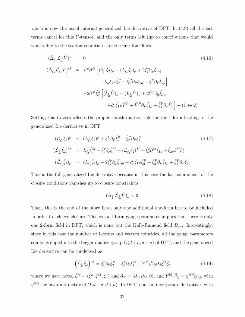
which is now the usual internal generalized Lie derivative of DFT. In (4.9) all the last
terms cancel for this Y -tensor, and the only terms left (up to contributions that would
vanish due to the section condition) are the first four lines
(∆ξ1Lξ2
V )µ = 0 (4.16)
(∆ξ1Lξ2
V )M = V µ∂M[
(δξ1 ξ2)µ − (Lξ1ξ2)µ + 2ξρ2∂[ρξ1µ]
−∂µξ1P ξP2 + ξP2 ∂P ξ1µ − ξP1 ∂P ξ2µ
]
−2∂M ξµ2
[
(δξ1 V )µ − (Lξ1V )µ + 2V ρ∂[ρξ1µ]
−∂µξ1P VP + V P∂P ξ1µ − ξP1 ∂P Vµ
]
+ (1 ↔ 2)
Setting this to zero selects the proper transformation rule for the 1-form leading to the
generalized Lie derivative in DFT
(Lξ1ξ2)
µ = (Lξ1ξ2)
µ + ξP1 ∂P ξµ2 − ξP2 ∂P ξ
µ1 (4.17)
(Lξ1ξ2)
M = Lξ1ξM2 − ξ
ρ2∂ρξ
M1 + (Lξ1
ξ2)M + ξ
ρ2∂
M ξ1ρ + ξ2ρ∂M ξ
ρ1
(Lξ1ξ2)µ = (Lξ1
ξ2)µ − 2ξρ2∂[ρξ1µ] + ∂µξ1P ξP2 − ξP2 ∂P ξ1µ + ξP1 ∂P ξ2µ
This is the full generalized Lie derivative because in this case the last component of the
closure conditions vanishes up to closure constraints
(∆ξ1Lξ2
V )µ = 0 (4.18)
Then, this is the end of the story here, only one additional one-form has to be included
in order to achieve closure. This extra 1-form gauge parameter implies that there is only
one 2-form field in DFT, which is none but the Kalb-Ramond field Bµν . Interestingly,
since in this case the number of 1-forms and vectors coincides, all the gauge parameters
can be grouped into the bigger duality group O(d+n, d+n) of DFT, and the generalized
Lie derivative can be condensed as
(
Lξ1ξ2
)
M = ξP1∂PξM2 − ξP2∂Pξ
M1 + Y M
PNQ∂Nξ
Q1 ξ
P2 (4.19)
where we have noted ξM = (ξµ, ξM , ξµ) and ∂M = (∂µ, ∂M , 0), and Y MPNQ = ηMNηPQ, with
ηMN the invariant metric of O(d+n, d+n). In DFT, one can incorporate derivatives with
32

respect to the form directions ∂µ, and constrain or completely eliminate their dependence
by imposing an external O(d, d) section condition. We expect that this is also the case in
the general case of U -duality groups, although in this paper we are setting them to zero
explicitly.
4.2.2 The E7(7) case
The above analysis fails to work for E7(7). The problem can already be tracked back to
equation (4.6). The reason is that the last term, while vanishing in the cases of O(n, n)
and En+1(n+1), n < 6, does not vanish when the Y -tensor is that of E7(7) because it
contains an antisymmetric piece
Y MPN
Q = −12PMN(PQ) +
1
2ωMNω[PQ] (4.20)
While the two extra terms in (4.7) cancel the failure of the first two terms in (4.6), there
is no obvious covariant completion to the generalized Lie derivative that would cancel the
last term in (4.6).
In close relation to this fact, although we have been able to close the algebra in the
compactified case, by adding the extra term in (3.5), there is no obvious covariant uplift
for this contribution, such that it compactifies to the form (3.8), namely, the new gauge
parameter contracted with the intertwining tensor. To be more specific, let us note that
the intertwining tensor F(AB)C can be cast as follows in terms of the twist matrix
F(AB)C = Y M
PN
Q∂NU(AQUB)
P (U−1)MC (4.21)
Then, starting from the last term in the third line of (3.31), it should uplift to
ξµABF(AB)
CUCM =
1
2Y M
PN
Q∂N ξµPQ + Y M
[PN
Q]∂NUAQUB
P ξµAB (4.22)
where we assume that the Scherk-Schwarz ansatz is of the form ξµPQ = UA
PUBQξµ
AB.
Clearly the uplift should not be U -dependent, and then we see again that the failure
to uplift the intertwining term in the reduced generalized Lie derivative is proportional
to Y M[P
NQ]. Then, the result is that without adding a new contribution to (4.7) or
33

supplementing it with some additional constraints, the closure fails to work up to terms
proportional to the antisymmetric part of the Y -tensor (4.9).
Already in [30] there were indications that the E7(7) case is special in this respect: while
the divergence of the 1-form gauge parameters is covariant (the connection contributions
vanish) for En+1(n+1) with n < 6, this is not the case of E7(7). More concretely, for n < 6
one has
Y MPN
Q∇NξµPQ = Y M
PN
Q∂NξµPQ (4.23)
and then this expression is connection free. Then, one possibility is that the extra-
contributions in (4.9) should be actually defined in terms of a covariant derivative. An-
other possibility is implementing a field section condition. As we will see in the next
section, when filling the fundamental 56 representation with the degrees of freedom of
11-dimensional maximal supergravity, only 28 components can be associated to gauge pa-
rameters of the theory. The rest correspond to gauge parameters that transform the fields
that couple to dual branes. Then, perhaps in this case the closure requires a duality co-
variant constraint of the form ωPQξP1 ξ
Q2 = 0, such that its solutions select a 28-dimensional
section of the parameter space, which would cancel the problematic last term in (4.6).
Also, it could be possible that even without a constraint of this form, one should sup-
plement the algebra with duality relations between gauge parameters. Analyzing these
possibilities lies beyond the scope of this paper, we leave this here as an open problem.
4.2.3 The En+1(n+1) case for n < 6
We now move to the other exceptional groups. In the case of En+1(n+1) with n < 6, the
internal Y -tensor is symmetric in the pairs of upper and lower indices Y M[P
NQ] = 0.
Then, in (4.9) the fifth and sixth lines vanish, and the first four determine the gauge
34

transformation of the new components6
Y MPN
Q∂N
(
Lξ1ξ2
)
µPQ = Y M
PN
Q∂N
[
Lξ1ξ2µ
PQ + 2ξρ2∂[µξ1ρ]PQ + 2∂µξ
Q1 ξ
P2 (4.24)
−2Y PRTS ξ
Q
[2∂T ξ1]µRS + (Lξ1
ξ2µPQ − Y P
RTS ξ
Q1 ∂T ξ2µ
RS)]
Notice that this expression is projected by the “intertwining” operator7
1
2Y M
PN
Q ∂N (. . . )PQ . (4.25)
We can then proceed as in the previous section, and remove the projection up to terms
that vanish under it
(
Lξ1ξ2
)
µ<MN> = Lξ1
ξ2µ<MN> + 2ξρ2∂[µξ1ρ]
<MN> + 2Y MPN
Q∂µξQ1 ξ
P2 + Γµ
<MN> (4.26)
−2Y MPN
QξQ
[2∂T ξ1]µ<PT> + Lξ1
ξ2µ<MN> − Y M
PN
QξQ1 ∂T ξ2µ
<PT>
We are using the notation that
ξµ<MN> = Y M
PN
QξµPQ (4.27)
and have then included Γµ<MN> which satisfies the relations
∂N Γµ<MN> = 0 , Γµ
<MN>∂N ϕ = 0 (4.28)
6 We used the identity
Y MPN
Q ∂T
(
Y PRTS ξ
Q1 ξ2µ
RS − ξT1 ξ2µPQ
)
∂N ϕµ
=
[
Y MPN
QξQ1 (Y P
RTS∂T ξ2µ
RS)− Lξ1(YM
PN
Qξ2µPQ)
−Y TRN
S ξ2µRS∂T ξ
M1 + Y N
PTQ∂T ξ
Q1 Y M
RPS ξ2µ
RS
+2∂T ξQ1 ξ2µ
RS(
Y MQ(N |
PYPR|T )
S − Y MR(N
SδT )Q
)
−4∂T ξQ1 ξ2µ
RSY M[Q
(N |P ]Y
PR|T )
S
]
∂N ϕµ
where the last three lines contain section condition-like terms that contribute to (4.10) to form clo-
sure constraints that compactify to the quadratic constraints in gauge maximal supergravity, and terms
antisymmetric in Y that are irrelevant in this subsection.7 We call it intertwining operator since it plays the same projection role as the intertwining tensors
(3.32) in the compactified case.
35

where ϕ represents any field or gauge parameter. As happens in the reduced case, Γµ<MN>
must be determined by demanding closure for this new component
(
∆ξ1Lξ2
V)
µ<MN> = 0 (4.29)
and this will require the new contributions to include the gauge parameters components
of the next step of the hierarchy, and so on.
Notice that the last two terms in (4.26) compactify to the (En+1(n+1), n < 6 analog
of the) first term in the fifth line of (3.31), which is proportional to the intertwining
tensor of the second level. Since the second term in that line is also proportional to this
intertwining tensor (contracted with the new 2-form component of the gauge parameters),
we can use the last two terms in (4.26) to determine what the next intertwining operator
will be. After some algebra one can show that for a symmetric Y -tensor, the following
identity holds
Y MPN
Q
(
Y PRTS ξ
Q1 ∂T ξ2µ
RS − Lξ1ξ2µ
PQ)
= ∂T (ξQ1 ξ2µ
RS)Y MNTQRS − 3ξ2µ
RS∂T ξQ1 Y
MNT(QRS) (4.30)
where we have defined
Y MNTQRS = Y M
PN
QYPRTS − Y M
RN
SδTQ (4.31)
The last term in (4.30) vanishes in the cases En+1(n+1) for n < 5 [14], but not for n = 5.
Then, at least for n < 5 and based on (4.7) one can conjecture that the Γµ<MN> will
contain contributions of the form
Γµ<MN> =
1
3
(
ξρ2∂T ξ1µρ
<MNT> + ξ2µρ<MNT>∂T ξ
ρ1
)
+ . . . (4.32)
where
ξµν<MNT> = Y MNT
QRS ξµνQRS (4.33)
and that the intertwining operator of the following level will read
1
3Y MNT
QRS ∂T (. . .)QRS (4.34)
36

Notice that in the O(n, n) case, the Y -tensor vanishes, and this explains why the tensor
hierarchy ends at the 1-form.
Let us note that the Y -tensor selects the correct representations for the 1-form vectors.
For the different U-duality groups En+1(n+1) it reads [14]
n = 2 : Y iαlδjβ
kγ = 4δijklδαβγδ
n = 3 : Y MPN
Q = ǫiMNǫiPQ
n = 4 : Y MPN
Q =1
2(γi)MN(γi)PQ
n = 5 : Y MPN
Q = 10dMNRdPQR (4.35)
where for n = 2, the SL(3) indices take values i, j = 1, 2, 3 and the SL(2) indices take
values α, β = 1, 2, for n = 3 the SL(5) indices take values i = 1, . . . , 5 and M = [ij],
for n = 4 the γ-matrices correspond to the 16 × 16 MW representation of SO(5, 5), so
i = 1, . . . , 10, and for n = 5 the d-tensor is the symmetric invariant of E6(6). Notice
that this tensor projects the 1-form components of the gauge parameters to the following
representations
Y MPN
QξµPQ =
n = 2 : 4ξµ[ij][αβ] (3, 1)
n = 3 : ǫiMNξµi 5
n = 4 : 12(γi)MNξµi 10
n = 5 : 10dMNRξµR 27
n = 6 : −12(tα)MNξµ
α + 12ωMNξµ 133 + 1
(4.36)
Accordingly, we expect the Y -tensor (4.31) to be related to the representations of the
2-form gauge parameters.
In the E6(6) case the obstruction is related to the fact that there is no clear uplift for
the (E6(6) analog of the) last component of the fifth line in (3.31). This obstruction in
the second level of E6(6) has the same origin of the obstruction at the first level of E7(7),
discussed around equation (4.22), and the way to circumvent them should proceed in the
same way as in the first level of E7(7). Notice however that since the first level of the
37

algebra closes in this case, one can write an action that includes the 2-form curvature of
the gauge fields, as in [34].
Let us now introduce the field degrees of freedom and compute the fluxes to see what
the implications of this will be in the construction of EFTs. Consider a generalized field-
dependent frame, in the spirit of (3.34)
EAM =
eaµ −ea
ρAρM ea
ρ(Bρµ<MN> − Aρ
<MAµN>)
0 ΦAM 2Aµ
<MΦAN>
0 0 (e−1)µaΦA
<MΦBN>
. . .
(4.37)
and define the generalized fluxes as
FABC = (LE
A
EB)M(E−1)M
C (4.38)
Just to put an example, they contain the 2-form curvature for the gauge fields
FabC = −ea
µebν(Φ−1)M
CFµνM (4.39)
with
FµνM = 2∂[µAν]
M − [[Aµ, Aν ]]M −
1
2Y M
PN
Q∂NBµνPQ (4.40)
where we have defined the internal exceptional C-bracket
[[Aµ, Aν ]] =1
2
(
LAµAν − LAν
Aµ
)
(4.41)
and assumed that the Y -tensor is symmetric. Since, at this level the algebra closes for
En+1(n+1), n < 6, it is possible to define a theory in terms of this curvature, as achieved
in [34] for E6(6).
The generalized frame above was written in a gauged fixed H = SO(1, d − 1) × Hi
triangular form (Hi is the local compact maximal subgroup of the U-duality group). Then,
in order to analyze the gauge transformations of its components, we must make sure that
the generalized diffeomorphic transformations preserve this gauge choice, by performing
38

a compensating H-transformation8. The combined transformations that preserve the
gauged-fixed form of the generalized frame read9
δ′EAM = LξEA
M − ΛABEB
M (4.42)
We will focus for simplicity in the transformation of the vielbein eaµ, gauge fields Aµ
M and
scalars ΦAM , but this analysis can be extended to the other components. In particular,
demanding that the ()21 component remains zero under a gauge transformation selects
ΛAb = −(e−1)µ
bΦAP∂P ξ
µ , ΛaB = ηabδ
AB(e−1)µbΦA
P∂P ξµ (4.43)
Notice that this compactifies to zero, which is the reason why no compensation of this
form was required in the previous section. Here we introduced the components of the
invariant SO(1, d− 1)×Hi metric, namely the flat Minkowski and Euclidean metrics ηab
and δAB. Then, we can readily find the gauge transformations of the components
δ′eaµ = Lξea
µ + ξP∂P eaµ + ea
ρAρP∂P ξ
µ (4.44)
δ′AµM = LξAµ
M + ∂µξM + LξAµ
M −1
2∂N ξµ
<MN>
−1
2(Bµρ
<MN> −Aµ<MAρ
N>)∂N ξρ − Aµ
P∂P ξρAρ
M + gµνMMP∂P ξ
ν
δ′ΦAM = LξΦA
M + LξΦAM + Aρ
<MΦAN>∂N ξ
ρ − AµMΦA
P∂P ξµ
where we have defined the internal “scalar” matrix MMN = ΦAMδABΦB
N and the “ex-
ternal” metric gµν = (e−1)µaηab(e
−1)νb.
For the sake of completeness, we now establish the redefinitions required to make
contact with the results in [34]. Regarding the fluxes, one can already see that the gauge
curvature (4.40) coincides. Focussing on the internal transformation of the gauge field
AµM , we find that redefining the 1-form gauge parameter as
1
2ξµ
<MN> = Ξµ<MN> + ξ<MAµ
N> (4.45)
8 Let us emphasize that actually this is not needed in our approach since by construction the frame
is indeed a collection of vectors, and therefore its transformation is well defined and independent of the
choice of frame.9 We note these transformation with δ′, to distinguish them from the transformations δ considered
before.
39

one obtains
δ′AµM = Dµξ
M − ∂N Ξµ<MN> , Dµ = ∂µ − LAµ
(4.46)
which is the internal gauge transformation of the gauge fields as exposed in [34]. There,
instead of considering purely external diffeomorphisms, the authors combined them with a
subsector of internal diffeos where the internal gauge parameters are restricted to the form
ξM = −ξνAνM , such that this particular combination results in gauge transformations
that look like external diffeomorphisms, but are manifestly covariantized with respect to
the gauge fields. To make contact with those transformations, one also has to make the
following redefinition
Ξµ<MN> → Ξµ
<MN> −1
2ξρ(Bµρ
<MN> − Aµ<MAN>
ρ ) (4.47)
and then the gauge transformations (4.44) reduce to
δ′eaµ = ξρDρea
µ − eaρDρξ
µ
δ′AµM = ξρHρµ + gµνM
MP∂P ξµ (4.48)
δ′ΦAM = ξρDρΦA
M
One could also extended this analysis for the 2-form field, were we expect the transfor-
mation to depend on its curvature, and then it seems that duality relations would be
required to make contact with [34]. It would be interesting to explore the role of dualities
of that type at the level of the algebra of generalized diffeomorphisms discussed here.
4.3 The gauge structure of the full generalized Lie derivative
Collecting the information from the previous subsections, we can now try to condense
the notation. As in the compactified case, the gauge parameters can be thought of as
components of a generalized gauge parameter in an extended mega-space
ξM = (ξµ, ξM , ξµ<MN>, ξµν
<MNP>, . . . ) (4.49)
One can then define a generalized Lie derivative that takes the form
(
Lξ1ξ2
)
M = ξP1∂PξM2 − ξP2∂Pξ
M1 + Y M
PNQ∂Nξ
Q1 ξ
P2 (4.50)
40
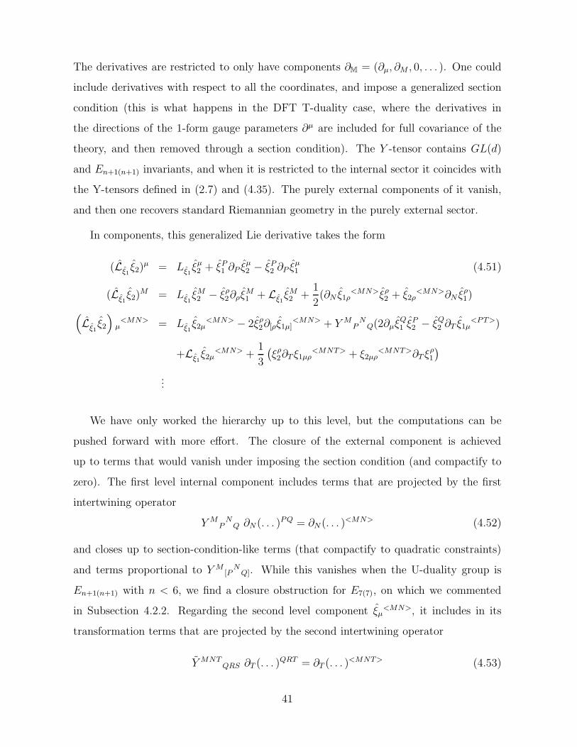
The derivatives are restricted to only have components ∂M = (∂µ, ∂M , 0, . . . ). One could
include derivatives with respect to all the coordinates, and impose a generalized section
condition (this is what happens in the DFT T-duality case, where the derivatives in
the directions of the 1-form gauge parameters ∂µ are included for full covariance of the
theory, and then removed through a section condition). The Y -tensor contains GL(d)
and En+1(n+1) invariants, and when it is restricted to the internal sector it coincides with
the Y-tensors defined in (2.7) and (4.35). The purely external components of it vanish,
and then one recovers standard Riemannian geometry in the purely external sector.
In components, this generalized Lie derivative takes the form
(Lξ1ξ2)
µ = Lξ1ξµ2 + ξP1 ∂P ξ
µ2 − ξP2 ∂P ξ
µ1 (4.51)
(Lξ1ξ2)
M = Lξ1ξM2 − ξ
ρ2∂ρξ
M1 + Lξ1
ξM2 +1
2(∂N ξ1ρ
<MN>ξρ2 + ξ2ρ
<MN>∂N ξρ1)
(
Lξ1ξ2
)
µ<MN> = Lξ1
ξ2µ<MN> − 2ξρ2∂[ρξ1µ]
<MN> + Y MPN
Q(2∂µξQ1 ξ
P2 − ξ
Q2 ∂T ξ1µ
<PT>)
+Lξ1ξ2µ
<MN> +1
3
(
ξρ2∂T ξ1µρ
<MNT> + ξ2µρ<MNT>∂T ξ
ρ1
)
...
We have only worked the hierarchy up to this level, but the computations can be
pushed forward with more effort. The closure of the external component is achieved
up to terms that would vanish under imposing the section condition (and compactify to
zero). The first level internal component includes terms that are projected by the first
intertwining operator
Y MPN
Q ∂N (. . . )PQ = ∂N (. . . )
<MN> (4.52)
and closes up to section-condition-like terms (that compactify to quadratic constraints)
and terms proportional to Y M[P
NQ]. While this vanishes when the U-duality group is
En+1(n+1) with n < 6, we find a closure obstruction for E7(7), on which we commented
in Subsection 4.2.2. Regarding the second level component ξµ<MN>, it includes in its
transformation terms that are projected by the second intertwining operator
Y MNTQRS ∂T (. . . )
QRT = ∂T (. . . )<MNT> (4.53)
41

The closure obstruction in this case is proportional to Y MNT(QRS). Now this vanishes for
n < 5, but not for E6(6), and this obstruction was commented in Subsection 4.2.3. We ex-
pect issues like this will appear at level 7−n for En+1(n+1), for the adjoint representations,
but this has to be explored further.
We have also shown how to introduce a field-dependent generalized frame and how
to extract the gauge transformations on its components, and how to build the covariant
quantities. These results will be useful when constructing full duality invariant Excep-
tional Field Theories.
5 Contact with 11-dimensional supergravity (and be-
yond)
In this section we concentrate on d = 4 and U-duality group E7(7). Using a GL(7) ⊂
SL(8) ⊂ E7 decomposition, were GL(7) acts on the “internal” tangent space in the
supergravity limit, i.e. on the coordinates dual to momentum, which can be either defined
by hand, or by a section condition. By this, we give the 11-dimensional origin of the gauge
parameters, external 1-forms and some of the 2-forms, etc. that we have seen. The same
can be done for type II theories, but we will skip it (all the information about the purely
internal objects can be found for example in [12]).
The exceptional generalized tangent space encodes all the gauge transformations of
11-dimensional supergravity, namely diffeomorphisms and gauge transformations of the
3-form field. In order to recover an electro-magnetic covariant formulation, we need
to include their duals, namely a 5-form corresponding to gauge transformations of the
6-form potential, and a gauge transformation for a “dual graviton”, transforming as a 7-
form times a 1-form [9]. The generalized tangent space can equivalently be constructed by
counting the charges of the theory, namely momentum, M2 and M5 brane charge, and KK
monopole charge (being the electric charge for the dual graviton). Furthermore, to build
the tensor hierarchy, or equivalently to go higher levels, more brane charges are needed,
corresponding to the so-called “U-branes” or “exotic branes” [42]-[44] (i.e. configurations
42

with non-trivial U-duality monodromies). For example, to reconstruct the 133 space-time
1-forms, we need to add the exotic branes termed 53 and 26 in [44] (see [42] for an earlier
discussion). These have no direct 11-dimensional interpretation, as they exist only in
spaces with 3 and 6 isometries respectively, and are obtained from the type IIA NS5
brane by a chain of dualities and uplift. They transform as an 8-form tensor, a 3-form
and 6-form respectively, and appear already when counting scalar degrees of freedom in
E8(8) [18]. The generalized tangent space is therefore locally
E =T ⊕ Λ2T ∗ ⊕ Λ5T ∗ ⊕ Λ7T ∗ ⊗ T ∗ ⊕ Λ8T ∗ ⊗ Λ3T ∗ ⊕ Λ8T ∗ ⊗ Λ6T ∗ ⊕ · · ·
p M2 M5 KK 53 26 · · ·
(5.1)
where T is 11-dimensional. The dots account for higher p-form representations. For
example, to obtain the 912 degrees of freedom that appear in space-time 2-forms, we need
extra forms transforming as 9-forms times some lower form. These show up in the l1
representation of E11 at fourth order [20].
Splitting T = T4 + T7 we get the GL(4) and GL(7) representations indicated in
Table1.10
The bosonic fields of 11-dimensional supergravity are the metric and the 3-form gauge
field. Again, in order to achieve 4-dimensional electro-magnetic invariance, we need to
include their duals, a 6-form field A6 and the dual graviton B, transforming as Λ8T ∗⊗T ∗
[18]. The “gauge field” whose electric charge are the exotic branes included so far, termed
A93 and A96 , should transform respectively as Λ9T ∗ ⊗ Λ3T ∗ and Λ9T ∗ ⊗ Λ6T ∗. Again, to
fill out the corresponding E7(7) representations at the level of space-time 3-forms and on,
we need to include higher p-forms. The GL(4) and GL(7) representations we obtain for
the bosonic fields are shown in table 2.
10There is a subtlety in counting degrees of freedom: the “dual branes” (KK, 53, 26, etc) exist only in
spaces with U(1) isometries. Their respective T ∗, Λ3T ∗ and Λ6T ∗ lie along these compact directions. We
have therefore excluded the possibility of placing 4-dimensional space-time indices along them. If on the
contrary we allow this possibility, the KK monopole would count as 50 1-form degrees of freedom, and
the total number of 1-forms would be 133 + 1, in accordance with the E11 results [20], while the total
number of 2-forms would be 912 + 56.
43

p M2 M5 KK 53 26 · · ·
GL(4) GL(7) total E7(7) repr
scalar 7 21 21 7 0 0 0 56 ξM ∈ 56
1-form 0 7 35 49 35 7 0 133 ξµα ∈ 133
2-form 0 1 35 147 245 49 · · · 477+· · · ξµνA ∈ 912
3-form 0 0 21 245 735 147 · · · 1148+· · · ξµνρA ∈ 133 + 8645
Table 1: GL(4) and GL(7) decomposition of the generalized tangent space. We give the number
of internal components.
g A3 A6 B A93 A96 · · ·
GL(4) GL(7) total E7(7) repr
scalar 28 35 7 0 0 0 0 70 ΦAM ∈ 133
1-form 7 21 21 7 0 0 0 56 AµM ∈ 56
2-form 0 7 35 49 35 7 0 133 Bµνα ∈ 133
3-form 0 1 35 147 245 49 · · · 477+· · · CµνρA ∈ 912
4-form 0 0 21 245 735 147 · · · 1148+· · · DµνλρA ∈ 133 + 8645
Table 2: GL(4) and GL(7) decomposition of the bosonic fields. B represents the dual graviton,
and A93 , A96 the gauge fields that couple electrically to the 53 and 26 branes.
It will be useful to find the embedding of the metric and 3-form field, as well as their
gauge transformations (diffeomorphisms and 2-forms) in terms of SL(8) representations.
For that, we use the following notation: a, b, ... = 1, .., 8 are indices in the fundamental
of SL(8), while m,n = 1, ..., 7 are in the fundamental of GL(7). Later on we will use
M = 1, ..., 11 to denote indices along eleven-dimensional space-time (i.e. M = (µ,m)).
The fundamental representation of E7(7) decomposes with respect to SL(8) into
56 = 28+ 28′ (5.2)
ξ = (ξab, ξab)
44

and the adjoint
133 = 63+ 70 (5.3)
Φ = (Φab,Φabcd)
where Φaa = 0 and Φabcd is fully antisymmetric. Finally, the 912 decomposes into
912 = 36+ 420+ 36′ + 420′ (5.4)
F = (F ab, F abcd, Fab, Fabc
d)
where F ba = F ab and F abcc = 0 and similarly for the objects with the indices down.
We can then embed the generators of diffeomorphisms v and two-form gauge trans-
formations λ2 of conventional 11-dimensional supergravity, whose different external com-
ponents are given in the first two columns in Table 1, in the following way
ξm8 = vm , ξmn = λmn ∈ 28+ 28′ ∈ 56
ξµ = vµ , ξµ8m = λµm ∈ 1+ 63 ∈ 1+ 133
ξ88µν = λµν ∈ 36 ∈ 912
(5.5)
The scalar, vector, 2-form and 3-form fields coming from the metric and A3 are em-
bedded as
Φmn = am
n , Φmnp8 = Amnp ∈ 70 ∈ 133
Aµm8 = aµ
m , Aµmn = Aµmn ∈ 28+ 28′ ∈ 56
Bµν8m = Aµνm ∈ 63 ∈ 133
Cµνρ88 = Aµνρ ∈ 36 ∈ 912
(5.6)
Given this, the first row of the generalized vielbein (3.34) for 11-dimensional supergravity
reads therefore
EaM = −ea
ρ(
− δµρ , [aρm]8 + Aρmn, [Aρµm + aρ
pApµm]8, [Aµνρ + aρ
pAµνp +13aρ
paqµAνpq]88,
[Aρ[mnAp]µν +13aρ
qAqµ[mAnp]ν +13Aρmna[µ
qAν]pq]8)
, (5.7)
where the superindex 8 completes the SL(8) representation (for example the second term
corresponds to M = m8).
45

One can now use the generalized Lie derivative (4.7) with parameters (5.5), applied
to this generalized vielbein and obtain the gauge transformations of the fields in 11-
dimensional supergravity. After some algebra, one can show that from (LξEa)µ and
(LξEa)M one recovers precisely the gauge transformations of 11-dimensional supergravity,
namely
δeaM = Lvea
M
δAµmn = LvAµmn + (dλ)µmn (5.8)
where Lv means the ordinary Lie derivative with parameter vM = (vµ, vm), and we have
used eam = ea
ρaρm.
Note that we have correctly reproduced the gauge transformations of 11-dimensional
supergravity using the generalized Lie derivative (4.51) which, as we have shown, does
not close at the first level for E7(7). This is so because the obstruction for closure goes
away when the gauge parameters and the fields are those of 11-dimensional supergravity.
Indeed, on the one hand they obviously satisfy the section condition. On the other, terms
involving Y M[P
NQ] = 1
2ωMNωPQ go away when contracted with gauge fields or gauge
parameters, as the only non-zero components of the latter are those with fundamental
indices P or Q = m8 or P = mn, and therefore vanish in the symplectic products.
Furthermore, it is not hard to show that restricting the generalized tangent space
to vectors and two-forms, i.e. for U = (u, λ), V = (v, ω), u, v ∈ T , λ, ω ∈ Λ2T ∗, the
generalized Lie derivative
LUV = (Luv, Luω − ιvdλ) (5.9)
closes without any need to introduce other forms.
6 Conclusions
We have addressed the construction of U-duality invariant generalized diffeomorphisms
for M-theory. Taking as a starting point the generalized Lie derivatives for the different
46

U-duality groups introduced in [13],[14], we explored the completion to the full external
plus internal space-time.
We began with the Scherk-Schwarz-type compactification ansatz leading to gauged
maximal supergravity, and specialized the analysis to the E7(7) case in 4-dimensions in
Section 3. Closure of the algebra is highly non-trivial and requires an extension of the
tangent space to include the so-called tensor hierarchy. The closure at each level of the
hierarchy dictates the transformation rules of the following level. There is also a hierarchy
of intertwining tensors, such that when a given level of the hierarchy is projected by the
corresponding intertwiner, the (projected) sub-algebra formed by it and the previous levels
closes. Interestingly, this procedure allowed us to build a full generalized Lie derivative
in the reduced case, that encodes all the gauge transformations of maximal supergravity
and the tensor hierarchy (3.30)-(3.31).
The field content is introduced through a generalized frame (3.34), in such a way that
the different components transform appropriately (3.35). This is a novel construction, in
which the different levels of the tensor hierarchy are embedded into different components
of a generalized frame, in analogy to what happens with the 2-form in DFT.We then define
generalized fluxes in terms of the generalized frame and Lie derivative (3.36), and show
that the different components correspond to covariant quantities in the theory (3.37):
curvatures, covariant derivatives, etc. Since the generalized Lie derivative closes, the
closure of the generalized fluxes define the BIs of the theory (3.39).
Encouraged by this construction, we then moved towards a full generalized Lie deriva-
tive on the extended space (4.50). Again, closure requires an extended tangent space to
accommodate the tensor hierarchy, and level by level the closure conditions dictate the
transformation rules of the next level. We identified the “intertwining operators” of the
first levels, which play a role analog to (and compactify to) the intertwining embedding
tensor in the reduced theory.
Intriguingly, we found closure obstructions at different levels of the hierarchy for dif-
ferent U-duality groups. Although we have commented on how they can be circumvented,
this issue deserves further study.
47

Let us finally comment on future lines of investigation. Regarding the reduced case of
Section 3, it would be interesting to construct a generalized geometry through covariant
derivatives, connections, torsion and curvatures. This is expected to give rise to an action
and equations of motion of a democratic formulation of maximal gauged supergravity.
This framework can also be used to explore non-geometry, and possible uplifts for the new
maximal gauged supergravities in [50]. Regarding the extended construction of Section 4,
it would be interesting to further explore mechanisms to achieve full closure, and apply the
generalized frame and flux techniques of section 3 to build covariant quantities and actions
of Exceptional Field Theories. A construction of an underlying generalized geometry with
generalized connections and curvatures would allow to systematically obtain the actions
and equations of motion.
Acknowledgments
We thank B. de Witt, J. Palmkvist, M. Shigemori, D. Waldram and specially A. Coimbra
for useful discussions and comments. G. A. thanks the ICTP and CERN for hospitality
during the completion of this work. D. M. and J. A. R. thank Institut de Physique
Theorique, CEA/Saclay, for hospitality. This work was partially supported by EPLANET,
CONICET, PICT-2012-513 and the ERC Starting Independent Researcher Grant 259133-
ObservableString.
References
[1] W. Siegel, “Superspace duality in low-energy superstrings,” Phys. Rev. D 48 (1993)
2826 [hep-th/9305073].
[2] C. Hull and B. Zwiebach, “Double Field Theory,” JHEP 0909 (2009) 099
[arXiv:0904.4664 [hep-th]].
C. Hull and B. Zwiebach, “The Gauge algebra of double field theory and Courant
brackets,” JHEP 0909, 090 (2009) [arXiv:0908.1792 [hep-th]].
48

O. Hohm, C. Hull and B. Zwiebach, “Background independent action for double field
theory,” JHEP 1007 (2010) 016 [arXiv:1003.5027 [hep-th]].
O. Hohm, C. Hull and B. Zwiebach, “Generalized metric formulation of double field
theory,” JHEP 1008, 008 (2010) [arXiv:1006.4823 [hep-th]].
O. Hohm and S. K. Kwak, “Frame-like Geometry of Double Field Theory,” J. Phys.
A 44 (2011) 085404 [arXiv:1011.4101 [hep-th]].
[3] G. Aldazabal, D. Marques and C. Nunez, “Double Field Theory: A Pedagogical
Review,” Class. Quant. Grav. 30, 163001 (2013) [arXiv:1305.1907 [hep-th]].
D. S. Berman and D. C. Thompson, “Duality Symmetric String and M-Theory,”
arXiv:1306.2643 [hep-th].
O. Hohm, D. Lust and B. Zwiebach, “The Spacetime of Double Field Theory: Review,
Remarks, and Outlook,” arXiv:1309.2977 [hep-th].
[4] N. Hitchin, “Generalized Calabi-Yau manifolds,” Quart. J. Math. Oxford Ser. 54
(2003) 281 [arXiv:math.dg/0209099].
M. Gualtieri, “Generalized Complex Geometry,” Oxford University DPhil thesis
(2004) [arXiv:math.DG/0401221].
[5] A. Coimbra, C. Strickland-Constable and D. Waldram, “Supergravity as Generalised
Geometry I: Type II Theories,” JHEP 1111 (2011) 091 [arXiv:1107.1733 [hep-th]].
[6] P. Koerber, “Lectures on Generalized Complex Geometry for Physicists,” Fortsch.
Phys. 59, 169 (2011) [arXiv:1006.1536 [hep-th]].
[7] M. Grana, R. Minasian, M. Petrini and D. Waldram, “T-duality, Generalized Ge-
ometry and Non-Geometric Backgrounds,” JHEP 0904 (2009) 075 [arXiv:0807.4527
[hep-th]].
[8] C. M. Hull, “Generalised Geometry for M-Theory,” JHEP 0707 (2007) 079
[hep-th/0701203].
[9] P. P. Pacheco and D. Waldram, “M-theory, exceptional generalised geometry and
superpotentials,” JHEP 0809 (2008) 123 [arXiv:0804.1362 [hep-th]].
49

[10] G. Dall’Agata, N. Prezas, H. Samtleben and M. Trigiante, “Gauged Supergravities
from Twisted Doubled Tori and Non-Geometric String Backgrounds,” Nucl. Phys. B
799 (2008) 80 [arXiv:0712.1026 [hep-th]].
[11] C. Hillmann, “Generalized E(7(7)) coset dynamics and D=11 supergravity,” JHEP
0903 (2009) 135 [arXiv:0901.1581 [hep-th]].
[12] G. Aldazabal, E. Andres, P. G. Camara and M. Grana, “U-dual fluxes and General-
ized Geometry,” JHEP 1011 (2010) 083 [arXiv:1007.5509 [hep-th]].
[13] A. Coimbra, C. Strickland-Constable and D. Waldram, “Ed(d) ×R+ Generalised Ge-
ometry, Connections and M theory,” arXiv:1112.3989 [hep-th].
A. Coimbra, C. Strickland-Constable and D. Waldram, “Supergravity as Generalised
Geometry II: Ed(d) × R+ and M theory,” arXiv:1212.1586 [hep-th].
[14] D. S. Berman, M. Cederwall, A. Kleinschmidt and D. C. Thompson, “The gauge
structure of generalised diffeomorphisms,” JHEP 1301 (2013) 064 [arXiv:1208.5884
[hep-th]].
[15] G. Aldazabal, W. Baron, D. Marques and C. Nunez, “The effective action of Double
Field Theory,” JHEP 1111 (2011) 052 [arXiv:1109.0290 [hep-th]].
D. Geissbuhler, “Double Field Theory and N=4 Gauged Supergravity,” JHEP 1111
(2011) 116 [arXiv:1109.4280 [hep-th]].
[16] D. S. Berman and M. J. Perry, “Generalized Geometry and M theory,” JHEP 1106
(2011) 074 [arXiv:1008.1763 [hep-th]].
D. S. Berman, H. Godazgar, M. J. Perry and P. West, “Duality Invariant Actions
and Generalised Geometry,” arXiv:1111.0459 [hep-th].
D. S. Berman, H. Godazgar, M. Godazgar and M. J. Perry, “The Local symmetries of
M-theory and their formulation in generalised geometry,” arXiv:1110.3930 [hep-th].
[17] H. Godazgar, M. Godazgar and M. J. Perry, “E8 duality and dual gravity,” JHEP
1306 (2013) 044 [arXiv:1303.2035 [hep-th]].
50

[18] C. Strickland-Constable, “Subsectors, Dynkin Diagrams and New Generalised Ge-
ometries,” arXiv:1310.4196 [hep-th].
[19] H. Samtleben and M. Weidner, “Gauging hidden symmetries in two dimensions,”
JHEP 0708, 076 (2007) [arXiv:0705.2606 [hep-th]].
[20] P. C. West, “E(11) and M theory,” Class. Quant. Grav. 18 (2001) 4443
[hep-th/0104081].
F. Riccioni and P. C. West, “The E(11) origin of all maximal supergravities,” JHEP
0707 (2007) 063 [arXiv:0705.0752 [hep-th]].
E. A. Bergshoeff, I. De Baetselier and T. A. Nutma, “E(11) and the embedding ten-
sor,” JHEP 0709, 047 (2007) [arXiv:0705.1304 [hep-th]].
F. Riccioni and P. C. West, “E(11)-extended spacetime and gauged supergravities,”
JHEP 0802 (2008) 039 [arXiv:0712.1795 [hep-th]].
P. West, “Generalised geometry, eleven dimensions and E11,” JHEP 1202, 018 (2012)
[arXiv:1111.1642 [hep-th]].
P. West, “E11, generalised space-time and equations of motion in four dimensions,”
JHEP 1212 (2012) 068 [arXiv:1206.7045 [hep-th]].
[21] F. Riccioni, D. Steele and P. West, “The E(11) origin of all maximal supergravities:
The Hierarchy of field-strengths,” JHEP 0909, 095 (2009) [arXiv:0906.1177 [hep-th]].
[22] J. Palmkvist, “Tensor hierarchies, Borcherds algebras and E11,” JHEP 1202 (2012)
066 [arXiv:1110.4892 [hep-th]].
[23] J. Palmkvist, “The tensor hierarchy algebra,” arXiv:1305.0018 [hep-th].
[24] J. Greitz, P. Howe and J. Palmkvist, “The tensor hierarchy simplified,”
arXiv:1308.4972 [hep-th].
[25] M. Henneaux, B. L. Julia and J. Levie, “E11, Borcherds algebras and maximal su-
pergravity,” JHEP 1204 (2012) 078 [arXiv:1007.5241 [hep-th]].
51

[26] D. S. Berman, E. T. Musaev, D. C. Thompson and D. C. Thompson, “Duality
Invariant M-theory: Gauged supergravities and Scherk-Schwarz reductions,” JHEP
1210 (2012) 174 [arXiv:1208.0020 [hep-th]].
[27] E. T. Musaev, “Gauged supergravities in 5 and 6 dimensions from generalised Scherk-
Schwarz reductions,” JHEP 1305 (2013) 161 [arXiv:1301.0467 [hep-th]].
[28] G. Aldazabal, M. Grana, D. Marques and J. A. Rosabal, “Extended geometry and
gauged maximal supergravity,” JHEP 1306, 046 (2013) [arXiv:1302.5419 [hep-th]].
[29] J. -H. Park and Y. Suh, “U-geometry : SL(5),” JHEP 04 (2013) 147 [arXiv:1302.1652
[hep-th]].
[30] M. Cederwall, J. Edlund and A. Karlsson, “Exceptional geometry and tensor fields,”
JHEP 1307 (2013) 028 [arXiv:1302.6736 [hep-th]].
[31] C. D. A. Blair, E. Malek and J. -H. Park, “M-theory and F-theory from a Duality
Manifest Action,” arXiv:1311.5109 [hep-th].
[32] O. Hohm and H. Samtleben, “Gauge theory of Kaluza-Klein and winding modes,”
Phys. Rev. D 88 (2013) 085005 [arXiv:1307.0039 [hep-th]].
[33] O. Hohm and H. Samtleben, “U-duality covariant gravity,” arXiv:1307.0509 [hep-th].
[34] O. Hohm and H. Samtleben, “Exceptional Form of D=11 Supergravity,”
arXiv:1308.1673 [hep-th].
O. Hohm and H. Samtleben, “Exceptional Field Theory I: E6(6) covariant Form of
M-Theory and Type IIB,” arXiv:1312.0614 [hep-th].
[35] B. de Wit, H. Samtleben and M. Trigiante, “The Maximal D=4 supergravities,”
JHEP 0706 (2007) 049 [arXiv:0705.2101 [hep-th]].
[36] B. de Wit, H. Samtleben and M. Trigiante, “On Lagrangians and gaugings of maximal
supergravities,” Nucl. Phys. B 655 (2003) 93 [hep-th/0212239].
[37] M. Weidner, “Gauged supergravities in various spacetime dimensions,” Fortsch. Phys.
55, 843 (2007) [hep-th/0702084].
52

[38] B. de Wit, H. Nicolai and H. Samtleben, “Gauged Supergravities, Tensor Hierarchies,
and M-Theory,” JHEP 0802, 044 (2008) [arXiv:0801.1294 [hep-th]].
[39] B. de Wit and H. Samtleben, “The End of the p-form hierarchy,” JHEP 0808 (2008)
015 [arXiv:0805.4767 [hep-th]].
[40] B. de Wit and M. van Zalk, “Supergravity and M-Theory,” Gen. Rel. Grav. 41 (2009)
757 [arXiv:0901.4519 [hep-th]].
[41] E. A. Bergshoeff, J. Hartong, O. Hohm, M. Huebscher and T. Ortin, “Gauge
Theories, Duality Relations and the Tensor Hierarchy,” JHEP 0904 (2009) 123
[arXiv:0901.2054 [hep-th]].
[42] C. M. Hull, “U duality and BPS spectrum of superYang-Mills theory and M theory,”
JHEP 9807, 018 (1998) [hep-th/9712075].
[43] E. A. Bergshoeff and F. Riccioni, “The D-brane U-scan,” arXiv:1109.1725 [hep-th].
[44] J. de Boer and M. Shigemori, “Exotic Branes in String Theory,” Phys. Rept. 532,
65 (2013) [arXiv:1209.6056 [hep-th]].
[45] M. Grana and D. Marques, “Gauged Double Field Theory,” JHEP 1204 (2012) 020
[arXiv:1201.2924 [hep-th]].
D. Geissbuhler, D. Marques, C. Nunez and V. Penas, “Exploring Double Field The-
ory,” JHEP 1306 (2013) 101 [arXiv:1304.1472 [hep-th]].
[46] G. Dibitetto, J. J. Fernandez-Melgarejo, D. Marques and D. Roest, “Duality orbits
of non-geometric fluxes,” Fortsch. Phys. 60 (2012) 1123 [arXiv:1203.6562 [hep-th]].
[47] O. Hohm and S. K. Kwak, “Double Field Theory Formulation of Heterotic Strings,”
JHEP 1106 (2011) 096 [arXiv:1103.2136 [hep-th]].
[48] D. S. Berman and K. Lee, “Supersymmetry for Gauged Double Field Theory and
Generalised Scherk-Schwarz Reductions,” arXiv:1305.2747 [hep-th].
[49] M. Grana and F. Orsi, “N=1 vacua in Exceptional Generalized Geometry,” JHEP
1108, 109 (2011) [arXiv:1105.4855 [hep-th]].
53

[50] G. Dall’Agata, G. Inverso and M. Trigiante, “Evidence for a family of SO(8) gauged
supergravity theories,” Phys. Rev. Lett. 109 (2012) 201301 [arXiv:1209.0760 [hep-
th]].
54