the fp420 r&d project: higgs and new physics with forward...
TRANSCRIPT

The FP420 R&D project: Higgs and New Physics with forward protons at the LHC
This article has been downloaded from IOPscience. Please scroll down to see the full text article.
2009 JINST 4 T10001
(http://iopscience.iop.org/1748-0221/4/10/T10001)
Download details:IP Address: 195.244.169.41The article was downloaded on 12/09/2011 at 14:19
Please note that terms and conditions apply.
View the table of contents for this issue, or go to the journal homepage for more
Home Search Collections Journals About Contact us My IOPscience
2009 JINST 4 T10001
PUBLISHED BY IOP PUBLISHING FOR SISSARECEIVED: December 31, 2008ACCEPTED: August 24, 2009PUBLISHED: October 1, 2009
TECHNICAL REPORT
The FP420 R&D project: Higgs and New Physics withforward protons at the LHC
FP420 R&D collaboration
M.G. Albrow,a R.B. Appleby,b M. Arneodo,c G. Atoian,d I.L. Azhgirey,e R. Barlow,bI.S. Bayshev,e W. Beaumont, f L. Bonnet,g A. Brandt,h P. Bussey,i C. Buttar,iJ.M. Butterworth, j M. Carter,k B.E. Cox,b,1 D. Dattola,l C. Da Via,m J. de Favereau,gD. d’Enterria,n P. De Remigis,l A. De Roeck,n, f ,1 E.A. De Wolf, f P. Duarte,h,2J.R. Ellis,n B. Florins,g J.R. Forshaw,m J. Freestone,m K. Goulianos,o J. Gronberg,pM. Grothe,q J.F. Gunion,r J. Hasi,m S. Heinemeyer,s J.J. Hollar,p S. Houston,iV. Issakov,d R.M. Jones,b M. Kelly,m C. Kenney,t V.A. Khoze,u S. Kolya,mN. Konstantinidis, j H. Kowalski,v H.E. Larsen,w V. Lemaitre,g S.-L. Liu,x A. Lyapine, jF.K. Loebinger,m R. Marshall,m A.D. Martin,u J. Monk, j I. Nasteva,m P. Nemegeer,gM.M. Obertino,c R. Orava,y V. O’Shea,i S. Ovyn,g A. Pal,h S. Parker,t J. Pater,mA.-L. Perrot,z T. Pierzchala,g A.D. Pilkington,m J. Pinfold,x K. Piotrzkowski,gW. Plano,m A. Poblaguev,d V. Popov,aa K.M. Potter,b F. Roncarolo,b A. Rostovtsev,aaX. Rouby,g M. Ruspa,c M.G. Ryskin,u A. Santoro,ac N. Schul,g G. Sellers,bA. Solano,w S. Spivey,h W.J. Stirling,u,3 D. Swoboda,z M. Tasevsky,ad R. Thompson,mT. Tsang,ab P. Van Mechelen, f A. Vilela Pereira,w S.J. Watts,m M.R.M. Warren, jG. Weiglein,u T. Wengler,m S.N. White,ab B. Winter,k Y. Yao,x D. Zaborov,aaA. Zampieri,l M. Zellerd and A. Zhokin f ,aa
aFermi National Accelerator Laboratory,Batavia, IL 60510, U.S.A.bUniversity of Manchester and Cockroft Institute,Manchester, M139PL, U.K.1Corresponding author.2Now at Rice University.3Now at Cambridge University, U.K. .
c! 2009 IOP Publishing Ltd and SISSA doi:10.1088/1748-0221/4/10/T10001

2009 JINST 4 T10001
cUniversita del Piemonte Orientale,Novara, Italy
dYale University,New Haven, CT 06520, U.S.A.eState Research Center of Russian Federation, IHEP,Protvino, Russiaf Universiteit Antwerpen,Antwerp, BelgiumgUniversite Catholique de Louvain,B-1348 Louvain-la-Neuve, BelgiumhUniversity of Texas at Arlington,Arlington TX 76019, U.S.A.iUniversity of Glasgow,Glasgow, G12 8QQ, U.K.jUniversity College London (UCL),London, WC1E 6BT, U.K.kMullard Space Science Laboratory (UCL),Holmbury St Mary, U.K.l INFN Torino,Torino, Italy
mUniversity of Manchester,Manchester, M139PL, U.K.nCERN, PH Department,CH-1211 Geneva 23, SwitzerlandoRockefeller University,New York NY 10021, U.S.A.pLawrence Livermore National Laboratory (LLNL),Livermore CA 94551, U.S.A.qUniversity of Wisconsin,Madison, WI 53706, U.S.A.rUniversity of California (Davis),Davis, CA 95616, U.S.A.sInstituto de Fisica de Cantabria,39005 Santander, SpaintMolecular Biology Consortium, Stanford University,Stanford CA 94305, U.S.A.uInstitute for Particle Physics Phenomenology,Durham, DH1 3LA, U.K.vDESY,D-22603 Hamburg, Germany
wUniversita di Torino and INFN,Torino, ItalyxUniversity of Alberta,Edmonton, T6G 2N5, Alberta, CanadayHelsinki Institute of Physics,FIN-00014, Helsinki, Finland

2009 JINST 4 T10001
zCERN, TS/LEA,CH-1211 Geneva 23, Switzerland
aaITEP,RU-117259, Moscow, Russia
abBrookhaven National Laboratory (BNL),Upton NY 11973, U.S.A.
acUniversidade do Estado do Rio de Janeiro (UERJ),BR-21945-970, Rio de Janeiro, Brasil
adInstitute of Physics,CZ-18221, Prague, Czech Republic
E-mail: [email protected], [email protected]
ABSTRACT: We present the FP420 R&D project, which has been studying the key aspects of thedevelopment and installation of a silicon tracker and fast-timing detectors in the LHC tunnel at420 m from the interaction points of the ATLAS and CMS experiments. These detectors wouldmeasure precisely very forward protons in conjunction with the corresponding central detectorsas a means to study Standard Model (SM) physics, and to search for and characterise new physicssignals. This report includes a detailed description of the physics case for the detector and, in partic-ular, for the measurement of Central Exclusive Production, pp" p+φ+ p, in which the outgoingprotons remain intact and the central system φ may be a single particle such as a SM or MSSMHiggs boson. Other physics topics discussed are γγ and γp interactions, and diffractive processes.The report includes a detailed study of the trigger strategy, acceptance, reconstruction efficiencies,and expected yields for a particular p p" pH p measurement with Higgs boson decay in the bbmode. The document also describes the detector acceptance as given by the LHC beam optics be-tween the interaction points and the FP420 location, the machine backgrounds, the new proposedconnection cryostat and the moving (“Hamburg”) beam-pipe at 420 m, and the radio-frequencyimpact of the design on the LHC. The last part of the document is devoted to a description of the3D silicon sensors and associated tracking performances, the design of two fast-timing detectorscapable of accurate vertex reconstruction for background rejection at high-luminosities, and thedetector alignment and calibration strategy.
KEYWORDS: Spectrometers; Particle tracking detectors; Cherenkov detectors; Timing detectors;Mass spectrometers
ARXIV EPRINT: 0806.0302
2009 JINST 4 T10001
Contents
1 Introduction 11.1 Executive summary 11.2 Outline 21.3 Integration of 420 m detectors into ATLAS and CMS forward physics programs 3
2 The physics case for Forward Proton Tagging at the LHC 32.1 Introduction 32.2 The theoretical predictions 52.3 Standard Model Higgs boson 62.4 h,H in the MSSM 8
2.4.1 h,H " bb decay modes 82.4.2 h,H " ττ decay modes 12
2.5 Observation of Higgs bosons in the NMSSM 122.6 Invisible Higgs boson decay modes 152.7 Conclusion of the studies of the CEP of h,H 152.8 Photon-photon and photon-proton physics 15
2.8.1 Introduction 152.8.2 Two-photon processes 172.8.3 Photon-proton processes 222.8.4 Photon-photon and photon-proton physics summary 25
2.9 Diffractive physics 262.9.1 Single diffractive production ofW , Z bosons or di-jets 282.9.2 Single diffractive and double pomeron exchange production of B mesons 282.9.3 Double pomeron exchange production ofW bosons 28
2.10 Physics potential of pT measurements in FP420 292.11 Other physics topics 31
2.11.1 Pomeron/graviton duality in AdS/CFT 312.11.2 Exotic new physics scenarios in CEP 31
3 Simulated measurement of h" bb in the MSSM 323.1 Trigger strategy for h" bb 343.2 Experimental cuts on the final state 353.3 Results and significances 373.4 Inclusion of forward detectors at 220 m 393.5 Comparison of the h,H " bb analyses 403.6 Recent improvements in background estimation 41
2009 JINST 4 T10001
4 LHC Optics, acceptance, and resolution 424.1 Introduction 424.2 Detector acceptance 444.3 Mass resolution 474.4 Optics summary 50
5 Machine induced backgrounds 505.1 Introduction 505.2 Near beam-gas background 515.3 Beam halo 52
5.3.1 Collimator settings and beam parameters 535.3.2 Beam halo induced by momentum cleaning collimators 545.3.3 Beam halo induced by betatron cleaning collimators 57
5.4 Halo from distant beam-gas interactions 575.5 Secondary interactions 58
5.5.1 Background particle fluxes and detector modeling 615.6 Machine background summary 62
6 A new connection cryostat at 420 m 636.1 Cryostat summary 66
7 Hamburg beam-pipe 677.1 Introduction 677.2 FP420 moving pipe design 687.3 Pocket design and tests 697.4 Test beam prototype 747.5 Motorization and detector system positioning 747.6 System operation and safeguards 757.7 Hamburg pipe summary and outlook 76
8 RF impact of Hamburg pipe on LHC 768.1 Motivation and introduction 768.2 Longitudinal impedance 77
8.2.1 Simulations 788.2.2 Laboratory measurements 78
8.3 Transverse impedance and beam instability 808.4 Coupling with detectors 818.5 RF summary 81
9 Silicon Tracking Detectors 829.1 Introduction 829.2 3D silicon detector development 839.3 Tracking detector mechanical support system 89
9.3.1 Superlayer and blade design 95

2009 JINST 4 T10001
9.3.2 Thermal tests of the blades 969.3.3 Assembly and alignment 969.3.4 Electrical details of the superplane 979.3.5 Station positioning 101
9.4 High-voltage and low-voltage power supplies 1019.4.1 Low-voltage power supplies specifications 1019.4.2 High-voltage power supplies specifications 1039.4.3 Power budget 1049.4.4 Low- and high-voltage channel count 1049.4.5 Temperature monitoring 1059.4.6 QUARTIC/GASTOF high- and low-voltage supplies 1059.4.7 Discussion of the solutions considered 1059.4.8 Summary of solutions 112
9.5 Readout and infrastructure at the host experiment 1129.5.1 CMS and ATLAS specific issues 1129.5.2 Tracker readout and downstream data acquisition 112
9.6 Thermal design 1139.6.1 Overview 1139.6.2 Thermal requirements 1159.6.3 Heat loads 1159.6.4 Heat flow 1169.6.5 Cold sink 118
9.7 Performance of the tracking system 119
10 Fast Timing Detectors 12510.1 Overlap background and kinematic constraints 12510.2 Timing 12510.3 Timing detectors 12710.4 Detector simulations 12910.5 Performance in test-beam measurements 13010.6 Electronics and data acquisition 13210.7 Reference time system 13310.8 Central detector timing 13510.9 Timing summary and future plans 136
11 Alignment and calibration 13811.1 Alignment requirements 138
11.1.1 Beam Position Monitors (BPMs) 13911.1.2 Wire Positioning Sensors (WPSs) 14011.1.3 The moving detectors 141
11.2 Beam and proton transfer calculations 14211.3 Machine alignment 14211.4 Mass scale and resolution measurement with physics processes 142
2009 JINST 4 T10001
11.5 Alignment summary 146
12 Near detector infrastructure and detector services 146
13 Conclusions 148
14 Costing 152
1 Introduction
1.1 Executive summary
Although forward proton detectors have been used to study Standard Model (SM) physics for a cou-ple of decades, the benefits of using proton detectors to search for New Physics at the LHC haveonly been fully appreciated within the last few years [1–6]. By detecting both outgoing protonsthat have lost less than 2% of their longitudinal momentum [7], in conjunction with a measure-ment of the associated centrally produced system using the current ATLAS and/or CMS detectors,a rich programme of studies in QCD, electroweak, Higgs and Beyond the Standard Model physicsbecomes accessible, with the potential to make unique measurements at the LHC. A prime processof interest is Central Exclusive Production (CEP), pp" p+φ+ p, in which the outgoing protonsremain intact and the central system φ may be a single particle such as a Higgs boson. In order todetect both outgoing protons in the range of momentum loss appropriate for central systems in the# 100 GeV/c2 mass range during nominal high-luminosity running, proton tagging detectors mustbe installed close to the outgoing beams in the high-dispersion region 420 m from the interactionpoints on each side of the ATLAS and CMS experiments. The FP420 R&D project is a collabora-tion including members from ATLAS, CMS, TOTEM and the accelerator physics community, withsupport from theorists, aimed at assessing the feasibility of installing such detectors.
The proposed FP420 detector system is a magnetic spectrometer. The LHC magnets betweenthe interaction points and the 420 m regions bend protons that have lost a small fraction of theirinitial momentum out of the beam envelope. The FP420 detector consists of a silicon trackingsystem that can be moved transversely and measures the spatial position of these protons relativeto the LHC beam line and their arrival times at several points in a 12 m region around 420 m. Theproposed instrumentation of the 420 m region includes the replacement of the existing 14 m longconnection cryostat with a warm beam-pipe section and a cryogenic bypass. To this purpose, anew connection cryostat has been designed, based on a modified arc termination module, so as tominimise the impact on the machine. The FP420 detector must be moveable because it should beparked at a large distance from the beams during injection and luminosity tuning, but must operateat distances between 4 mm and 7 mm from the beam centre during data taking, depending on thebeam conditions. A measurement of the displacement and angle of the outgoing protons relativeto the beam allows the momentum loss and transverse momentum of the scattered protons to bereconstructed. This in turn allows the mass of the centrally produced system φ to be reconstructed
– 1 –

2009 JINST 4 T10001
by the missing mass method [1] with a resolution (σ) between 2GeV/c2 and 3GeV/c2 per eventirrespective of the decay products of the central system.
The detector position relative to the beam can be measured both by employing beam positionmonitors and by using a high-rate physics process which produces protons of a known momentumloss (from a central detector measurement of the central system) in the FP420 acceptance range.The second method has the advantage that the magnetic field between the central detectors andFP420 does not have to be precisely known a priori.
The cross sections for CEP of the SM Higgs boson and other new physics scenarios are ex-pected to be small, on the femtobarn scale. FP420 must therefore be designed to operate up tothe highest LHC instantaneous luminosities of 1034cm$2s$1, where there will be on average 35overlap interactions per bunch crossing (assuming σtot = 110 mb). These overlap events can resultin a large fake background, consisting of a central system from one interaction and protons fromother interactions in the same bunch crossing. Fortunately, there are many kinematic and topolog-ical constraints which offer a large factor of background rejection. In addition, a measurement ofthe difference in the arrival times of the two protons at FP420 in the 10 picosecond range allowsfor matching of the detected protons with a central vertex within #2 mm, which will enable therejection of most of the residual overlap background, reducing it to a manageable level.
Studies presented in this document show that it is possible to install detectors in the 420 mregion with no impact on the operation or luminosity of the LHC (section 9). These detectors can becalibrated to the accuracy required to measure the mass of the centrally produced system to between2 and 3GeV/c2. This would allow an observation of new particles in the 60$ 180GeV/c2 massrange in certain physics scenarios during 3 years of LHC running at instantaneous luminosities of2% 1033 cm$2 s$1, and in many more scenarios at instantaneous luminosities of up to 1034 cm$2
s$1. Events can be triggered using the central detectors alone at Level 1, using information fromthe 420 m detectors at higher trigger levels to reduce the event rate. Observation of new particleproduction in the CEP channel would allow a direct measurement of the quantum numbers of theparticle and an accurate determination of the mass, irrespective of the decay channel of the particle.In some scenarios, these detectors may be the primary means of discovering new particles at theLHC, with unique ability to measure their quantum numbers. There is also an extensive, high-rateγγ and γp baseline physics program.
Similar detectors can also be installed at about 220 m, in a non-cryogenic region, and willincrease the acceptance to higher masses. In this paper we focus on the 420 m region.
We therefore conclude that the addition of such detectors will, for a relatively small cost,enhance the discovery and physics potential of the ATLAS and CMS experiments.
1.2 Outline
The outline of this document is as follows. In section 2 we provide a brief overview of the physicscase for FP420. In section 3 we describe in detail a physics and detector simulation of a particularscenario which may be observable if 420 m detectors are installed. The acceptance and massresolutions used in this analysis are presented in section 4. In section 5 we describe the machine-induced backgrounds at 420 m such as beam-halo and beam-gas backgrounds. We then turn tothe hardware design of FP420. Section 6 describes the new 420 m connection cryostat which willallow moving near-beam detectors with no effects on LHC operations. The design of the beam pipe
– 2 –

2009 JINST 4 T10001
in the FP420 region and the movement mechanism are described in section 7, and the studies of theradio-frequency impact of the design on the LHC are described in section 8. Section 9 describes thedesign of the FP420 3D silicon sensors, detectors and detector housings and off-detector servicessuch as cabling and power supplies. Section 10 describes two complementary fast timing detectordesigns, both of which are likely to be used at FP420. Section 11 describes the alignment andcalibration strategy, using both physics and beam position monitor techniques. We present ourconclusions and future plans in section 13.
1.3 Integration of 420 m detectors into ATLAS and CMS forward physics programs
This report focuses primarily on the design of 420 m proton tagging detectors. CMS will haveproton taggers installed at 220 m around its IP at startup, provided by the TOTEM experiment andfor which common data taking with CMS is planned [8]. ATLAS also has an approved forwardphysics experiment, ALFA, with proton taggers at 240m designed to measure elastic scattering inspecial optics runs [9].
There are ideas to upgrade the currently approved TOTEM detectors and a proposal to installFP420-like detectors at 220 m around ATLAS [10]. Adding detectors at 220 m capable of operatingat high luminosity increases the acceptance of FP420 for central masses of #120 GeV/c2 andupwards, depending on the interaction point1 and the distance of approach of both the 220 m and420 m detectors to the beam (see section 4). Throughout this document we present results for 420 mdetectors alone and where appropriate for a combined 220 m + 420 m system. It is envisaged thatFP420 collaboration members will become parts of the already existing ATLAS and CMS forwardphysics groups, and will join with them to propose forward physics upgrade programmes that willbe developed separately by ATLAS and CMS, incorporating the findings of this report.
2 The physics case for Forward Proton Tagging at the LHC
2.1 Introduction
A forward proton tagging capability can enhance the ability of the ATLAS and CMS detectors tocarry out the primary physics program of the LHC. This includes measurement of the mass andquantum numbers of the Higgs boson, should it be discovered via traditional searches, and aug-menting the discovery reach if nature favours certain plausible beyond the Standard Model scenar-ios, such as its minimal supersymmetric extension (MSSM). In this context, the central exclusiveproduction (CEP) of new particles offers unique possibilities, although the rich photon-photon andphoton-proton physics program also delivers promising search channels for new physics. Thesechannels are described in section 2.8.
By central exclusive production we refer to the process pp" p+ φ+ p, where the ‘+’ signsdenote the absence of hadronic activity (that is, the presence of a rapidity gap) between the outgoingprotons and the decay products of the central system φ. The final state therefore consists solely ofthe two outgoing protons, which we intend to detect in FP420, and the decay products of the centralsystem which will be detected in the ATLAS or CMS detectors. We note that gaps will not typicallybe part of the experimental signature due to the presence of minimum bias pile-up events, which
1For 220 m detectors, the acceptance is different around IP1 (ATLAS) and IP5 (CMS).
– 3 –

2009 JINST 4 T10001
Figure 1. Central Exclusive Production (CEP): pp" p+H+ p.
fill in the gap but do not affect our ability to detect the outgoing protons. Of particular interestis the production of Higgs bosons, but there is also a rich and more exotic physics menu thatincludes the production of many kinds of supersymmetric particles, other exotica, and indeed anynew object which has 0++ (or 2++) quantum numbers and couples strongly to gluons [2, 11] or tophotons [12]. The CEP process is illustrated for Higgs boson production in figure 1. The Higgsboson is produced as usual through gluon-gluon fusion, while another colour-cancelling gluon isexchanged, and no other particles are produced.
There are three important reasons why CEP is especially attractive for studies of new heavyobjects. Firstly, if the outgoing protons remain intact and scatter through small angles then, toa very good approximation, the primary active di-gluon system obeys a Jz = 0, C-even, P-even,selection rule [13]. Here Jz is the projection of the total angular momentum along the proton beamaxis. This selection rule readily permits a clean determination of the quantum numbers of any newresonance, which is predominantly 0++ in CEP. Secondly, because the process is exclusive, theenergy loss of the outgoing protons is directly related to the invariant mass of the central system,allowing an excellent mass measurement irrespective of the decay mode of the central system.Even final states containing jets and/or one or more neutrinos are measured with σM # 2GeV/c2.Thirdly, in many topical cases and in particular for Higgs boson production, a signal-to-backgroundratio of order 1 or better is achievable [14–18]. This ratio becomes significantly larger for Higgsbosons in certain regions of MSSM parameter space [15, 19, 20].
There is also a broad, high-rate QCD and electro-weak physics program; by tagging both ofthe outgoing protons, the LHC is effectively turned into a gluon-gluon, photon-proton and photon-photon collider [6, 21]. In the QCD sector, detailed studies of diffractive scattering, skewed, unin-tegrated gluon densities and the rapidity gap survival probability [2, 22–24] can be carried out. Inaddition, CEP would provide a source of practically pure gluon jets, turning the LHC into a ‘gluonfactory’ [13] and providing a unique laboratory in which to study the detailed properties of gluonjets, especially in comparison with quark jets. Forward proton tagging also provides unique ca-pabilities to study photon-photon and photon-proton interactions at centre-of-mass energies neverreached before. Anomalous top production, anomalous gauge boson couplings, exclusive dileptonproduction, or quarkonia photoproduction, to name a few, can be studied in the clean environmentof photon-induced collisions.
In what follows we will give a brief overview of the theoretical predictions including a surveyof the uncertainties in the expected cross sections. We will then review the possibilities of observingHiggs bosons in the Standard Model, MSSM and NMSSM for W , τ and b-quark decay channels.
– 4 –

2009 JINST 4 T10001
A major potential contribution of FP420 to the LHC program is the possibility to exploit the bbdecay channel of the Higgs particle, which is not available to standard Higgs analyses due tooverwhelming backgrounds. The combination of the suppression of the bb background, due tothe Jz = 0 selection rule, and the superior mass resolution of the FP420 detectors opens up thepossibility of exploiting this high branching ratio channel. Although the penalty for demanding twoforward protons makes the discovery of a Standard Model Higgs boson in the bb channel unlikelydespite a reasonable signal-to-background ratio, the cross section enhancements in other scenariosindicate that this could be a discovery channel. For example, it has recently been shown that theheavy CP-even MSSM Higgs boson, H , could be detected over a large region of the MA$ tanβplane; for MA # 140GeV/c2, discovery of H should be possible for all values of tan β. The 5σdiscovery reach extends beyond MA = 200GeV/c2 for tan β> 30 [19, 25]. We discuss the MSSMHiggs bosons measurements in the bb decay channel in detail in section 2.4.
In addition, for certain MSSM scenarios, FP420 provides an opportunity for a detailed line-shape analysis [15, 26]. In the NMSSM, the complex decay chain h" aa" 4τ becomes viable inCEP, and even offers the possibility to measure the mass of the pseudoscalar Higgs boson [27]. An-other attractive feature of the FP420 programme is the ability to probe the CP-structure of the Higgssector either by measuring directly the azimuthal asymmetry of the outgoing tagged protons [28]or by studying the correlations between the decay products [26].
2.2 The theoretical predictions
In this section we provide a very brief overview of the theoretical calculation involved in makingpredictions for CEP. We shall, for the sake of definiteness, focus upon Higgs boson production. Amore detailed review can be found in [5]. Referring to figure 1, the dominant contribution comesfrom the region Λ2QCD & Q2 &M2
h and hence the amplitude may be calculated using perturbativeQCD techniques [13, 29]. The result is
Ah ' NZ dQ2
Q6Vh fg(x1,x(1,Q2,µ2) fg(x2,x(2,Q2,µ2), (2.1)
where the gg" h vertex factor for the 0+ Higgs boson production is (after azimuthal-averaging)Vh ' Q2 and the normalization constant N can be written in terms of the h" gg decay width [2,29]. Equation (2.1) holds for small transverse momenta of the outgoing protons, although includingthe full transverse momentum dependence is straightforward [15, 30].
The fg’s are known as ‘skewed unintegrated gluon densities’ [31, 32]. They are evaluated atthe scale µ, taken to be #Mh/2. Since (x( # Q/
)s) & (x#Mh/
)s) & 1, it is possible to express
fg(x,x(,Q2,µ2), to single logarithmic accuracy, in terms of the gluon distribution function g(x,Q2).The fg’s each contain a Sudakov suppression factor, which is the probability that the gluons whichfuse to make the central system do not radiate in their evolution from Q up to the hard scale. Theapparent infrared divergence of Equation (2.1) is nullified by these Sudakov factors and, for theproduction of Jz = 0 central systems with invariant mass above 50GeV/c2, there is good control ofthe unknown infrared region of QCD.
Perturbative radiation associated with the gg" h subprocess, which is vetoed by the Sudakovfactors, is not the only way to populate and to destroy the rapidity gaps. There is also the possibility
– 5 –

2009 JINST 4 T10001
of soft rescattering in which particles from the underlying proton-proton event (i.e. from other par-ton interactions) populate the gaps. The production of soft secondaries caused by the rescattering isexpected to be almost independent of the short-distance subprocess and therefore can be effectivelyaccounted for by a multiplicative factor S2, usually termed the soft gap survival factor or survivalprobability [33]. The value of S2 is not universal and depends on the centre-of-mass energy of thecollision and the transverse momenta, pT , of the outgoing forward protons; the most sophisticatedof the models for gap survival use a two [23] and three-channel [22] eikonal model incorporatinghigh mass diffraction. To simplify the discussion it is common to use a fixed value correspondingto the average over the pT acceptance of the forward detectors (for a 120GeV/c2 Higgs boson, S2
is about 0.03 at the LHC). Taking this factor into account, the calculation of the production crosssection for a 120 GeV/c2 Standard Model Higgs boson via the CEP process at the LHC yields acentral value of 3 fb.
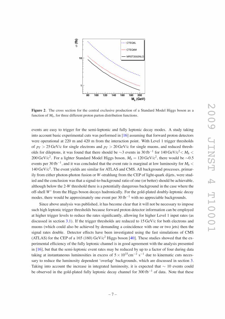
The primary uncertainties in the predicted cross section come from two sources. Firstly, sincethe gluon distribution functions g(x,Q2) enter to the fourth power, the predictions are sensitive tothe choice of parton distribution function (PDF) in the proton and in particular to the gluon den-sities at x = O(0.01). These are currently obtained from fits to data from HERA and the Tevatron.Figure 2 shows the prediction for the cross section for the CEP of a SM Higgs boson as a functionof Mh for three different choices of PDF at the LHC [20]. The cross section varies from 2.8 fb to11 fb for a 120 GeV/c2 SM Higgs boson, although the highest prediction comes from a leading or-der PDF choice and, since the calculation includes an NLO K-factor (K=1.5), one might concludethat this choice is the least favoured. Secondly, there is some uncertainty in the calculation of thesoft survival factor S2. Until recently, the consensus was that S2 has a value between 2.5% and4% at LHC energies [34], but a lower value has been discussed [24, 35] (although these have beenchallenged in [22]). Early LHC data on various diffractive processes — exclusive vector mesonphotoproduction, diffractive W production and central exclusive 2- and 3-jets production — willprovide respectively strong constraints on the gap survival factor, the unintegrated gluon distribu-tion and the Sudakov factor used in the theoretical calculations of the CEP Higgs cross section [36].
The reliability of the theoretical calculations can be checked to some extent at the Tevatron.The CDF collaboration has observed a 6σ excess of events in the exclusive dijet sample, pp"p+ j j+ p [37], which is well described by the theory. CDF has also observed several candidatesfor central exclusive di-photon production, pp" p+ γγ+ p [38] and measured scalar quarkoniumstates pp " p+ χc0 + p [39] at the predicted rates, although the invariant mass of the centralsystems are O(3-10 GeV/c2) and the infrared region may not be under good control. Both of thesepredictions include calculations for the soft survival factor at Tevatron energies.
The CDF measurements give some confidence in the predicted cross sections at the LHC.However, the theoretical uncertainties are approximately a factor of three, giving a predicted crosssection range for a 120 GeV/c2 SM Higgs boson of 1 to 9 fb.
2.3 Standard Model Higgs boson
The calculations of the previous section give a central cross section value of 3 fb for a 120 GeV/c2
SM Higgs boson, falling to 1 fb for a mass of 200 GeV/c2 (figure 2, where we take the more con-servative case obtained with the MRST PDFs). Out of the two dominant decay channels (h" bb,WW *), theWW * channel is the simplest way to observe the SM Higgs boson in CEP because the
– 6 –
2009 JINST 4 T10001
(GeV)hM80 100 120 140 160 180 200
(fb)
σ
1
10
CTEQ6L
CTEQ6M
MRST2002NLO
Figure 2. The cross section for the central exclusive production of a Standard Model Higgs boson as afunction ofMh, for three different proton parton distribution functions.
events are easy to trigger for the semi-leptonic and fully leptonic decay modes. A study takinginto account basic experimental cuts was performed in [16] assuming that forward proton detectorswere operational at 220 m and 420 m from the interaction point. With Level 1 trigger thresholdsof pT > 25GeV/c for single electrons and pT > 20GeV/c for single muons, and reduced thresh-olds for dileptons, it was found that there should be #3 events in 30 fb$1 for 140GeV/c2<Mh <
200GeV/c2. For a lighter Standard Model Higgs boson, Mh = 120GeV/c2, there would be #0.5events per 30 fb$1, and it was concluded that the event rate is marginal at low luminosity for Mh <
140GeV/c2. The event yields are similar for ATLAS and CMS. All background processes, primar-ily from either photon-photon fusion orW -strahlung from the CEP of light-quark dijets, were stud-ied and the conclusion was that a signal-to-background ratio of one (or better) should be achievable,although below the 2-W threshold there is a potentially dangerous background in the case where theoff-shellW * from the Higgs boson decays hadronically. For the gold-plated doubly-leptonic decaymodes, there would be approximately one event per 30 fb$1 with no appreciable backgrounds.
Since above analysis was published, it has become clear that it will not be necessary to imposesuch high leptonic trigger thresholds because forward proton detector information can be employedat higher trigger levels to reduce the rates significantly, allowing for higher Level 1 input rates (asdiscussed in section 3.1). If the trigger thresholds are reduced to 15GeV/c for both electrons andmuons (which could also be achieved by demanding a coincidence with one or two jets) then thesignal rates double. Detector effects have been investigated using the fast simulations of CMS(ATLAS) for the CEP of a 165 (160) GeV/c2 Higgs boson [40]. These studies showed that the ex-perimental efficiency of the fully leptonic channel is in good agreement with the analysis presentedin [16], but that the semi-leptonic event rates may be reduced by up to a factor of four during datataking at instantaneous luminosities in excess of 5% 1033cm$2 s$1 due to kinematic cuts neces-sary to reduce the luminosity dependent ‘overlap’ backgrounds, which are discussed in section 3.Taking into account the increase in integrated luminosity, it is expected that # 10 events couldbe observed in the gold-plated fully leptonic decay channel for 300 fb$1 of data. Note that these
– 7 –

2009 JINST 4 T10001
events have the striking characteristic of a dilepton vertex with no additional tracks, allowing forexcellent background suppression and affording a measurement of the Higgs mass to within #2GeV/c2 (the mass measurement by FP420 is not affected by the two undetected neutrinos). For a120 GeV/c2 Higgs boson, there will be a total of 5 events for 300 fb$1.
The conclusion is that the CEP of a SM Higgs boson should be observable in theWW * decaychannel for all masses in 300 fb$1 with a signal to background ratio of one or better. This willprovide confirmation that any observed resonance is indeed a scalar with quantum numbers 0++,and allow for a mass measurement2 on an event-by-event basis of better than 3GeV/c2 even in thedoubly-leptonic decay channels in which there are two final state neutrinos. This will be a vitallyimportant measurement at the LHC, where determining the Higgs quantum numbers is extremelydifficult without CEP. Furthermore, in certain regions of MSSM parameter space, in particularfor 140GeV/c2< MA < 170GeV/c2 and intermediate tanβ, the CEP rate for h"WW * may beenhanced by up to a factor of four [19]. We discuss the MSSM in more detail in the followingsection for the bb decay channel.
For the Standard Model Higgs boson, the bb decay channel is more challenging. It is theconclusion of [8, 20] that this channel will be very difficult to observe for Mh = 120GeV/c2 usingFP420 alone, but may be observable at the 3σ level if 220 m detectors are used in conjunctionwith FP420 and the cross sections are at the upper end of the theoretical expectations and/or theexperimental acceptance and trigger and b-tagging efficiencies are improved beyond the currentlyassumed values. This should not be dismissed, because such an observation would be extremelyvaluable, since there may be no other way of measuring the b-quark couplings of the SM Higgs atthe LHC.We discuss the experimental approach to observing Higgs bosons in the bb decay channelin detail in section 3.
2.4 h,H in the MSSM
In manyMSSM scenarios, the additional capabilities brought to the LHC detectors by FP420 wouldbe vitally important for the discovery of the Higgs bosons3 and the measurement of their proper-ties. The coupling of the lightest MSSM Higgs boson to b quarks and τ leptons may be stronglyenhanced at large tan β and small MA, opening up both modes to FP420. The cross sections maybecome so large in CEP that one could carry out a lineshape analysis to distinguish between differ-ent models [15, 26] and to make direct observations of CP violation in the Higgs sector [26, 28].If the widths are a few GeV/c2, a direct width measurement may be possible, a unique capabilityof FP420.
2.4.1 h,H " bb decay modes
In [19] (Heinemeyer et al.) a detailed study of the additional coverage in the MA$ tanβ planeafforded by FP420 and 220 m detectors was carried out for several benchmark MSSM scenarios.In particular, the observation of the CP-even Higgs bosons (h, H) in the b-quark decay channel wasinvestigated. Figure 3 shows the ratio of the MSSM to SM cross sections % the branching-ratio forthe h" bb channel within the Mmax
h scenario [41] as a function of MA and tanβ. For example, at2The mass resolution of FP420 is discussed in detail in section 4.3Here we are dealing with the lightest MSSM Higgs boson h and the heavier state H. Note that production of the
pseudo-scalar Higgs, A, is suppressed in CEP due to the Jz = 0 selection rule.
– 8 –

2009 JINST 4 T10001
[GeV]Am100 120 140 160 180 200 220 240
βta
n
5
10
15
20
25
30
35
40
45
50
= 115 GeV
hM
= 125 GeVhM
= 130 GeV hM
= 131 GeVhM
R = 1
R = 2
R = 5
R =
10 R =
15
Figure 3. The ratio, R, of cross section % branching ratio in the CEP h" bb channel in theMA - tanβ planeof theMSSMwithin theMmax
h benchmark scenario (with µ= +200GeV) to the SMHiggs cross section [19].The dark shaded (blue) region corresponds to the parameter region that is excluded by the LEP Higgs bosonsearches [42, 43].
tanβ= 33 andMA = 120GeV/c2, the cross section for h" bb in the MSSM is enhanced by a factorof five with respect to the Standard Model. The results shown are for µ= +200GeV, where theparameter µ determines the size and effect of higher order corrections; negative (positive) µ leadsto enhanced (suppressed) bottom Yukawa couplings.
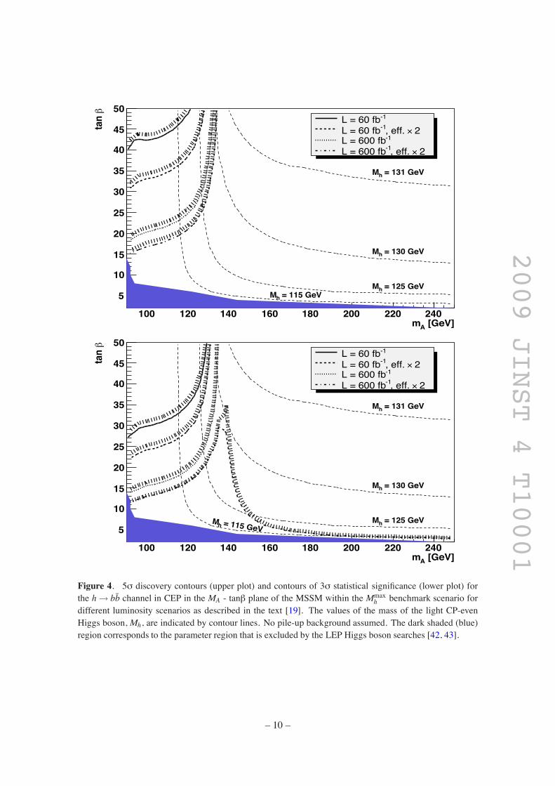
Figure 4 shows the 5σ discovery contours (upper plot) and the 3σ contours (lower plot) forthis scenario. The discovery contours were calculated using an experimental efficiency based on thesimulated analysis in the CMS-TOTEM studies [8], with a full simulation of the acceptance of bothFP420 and 220 m forward proton detectors. The Level 1 trigger strategy was based on informationonly from the central detectors and 220 m detectors. Full details can be found in [19]. Curvesare shown for several luminosity scenarios;
R
L = 60 fb$1 corresponds to 3 years of data takingby ATLAS and CMS at 1033 cm$2 s$1, and
R
L = 600 fb$1 corresponds to 3 years of data takingby both experiments at 1034 cm$2 s$1. For example, if tanβ = 40 and MA = 120GeV/c2, h" bbwould be observed with more than 3σ confidence with 60 fb$1 of data (lower plot), but wouldrequire twice the experimental efficiency or more integrated luminosity to be observed with 5σconfidence (upper plot). Figure 5 shows the 5σ discovery contours (upper plot) and the 3σ contours(lower plot) for the heavy scalar, H , in the same scenario. With sufficient integrated luminosity (fewhundreds fb$1), all values of tanβ are covered for MA # 140GeV/c2 and at high tanβ observationremains possible for Higgs bosons with masses in excess of 200GeV/c2.
– 9 –
2009 JINST 4 T10001
[GeV]Am100 120 140 160 180 200 220 240
βta
n
5
10
15
20
25
30
35
40
45
50
= 115 GeV hM = 125 GeVhM
= 130 GeVhM
= 131 GeVhM
-1L = 60 fb 2 ×, eff. -1L = 60 fb
-1L = 600 fb 2 ×, eff. -1L = 600 fb
[GeV]Am100 120 140 160 180 200 220 240
βta
n
5
10
15
20
25
30
35
40
45
50
= 115 GeV hM = 125 GeVhM
= 130 GeVhM
= 131 GeVhM
-1L = 60 fb 2 ×, eff. -1L = 60 fb
-1L = 600 fb 2 ×, eff. -1L = 600 fb
Figure 4. 5σ discovery contours (upper plot) and contours of 3σ statistical significance (lower plot) forthe h" bb channel in CEP in the MA - tanβ plane of the MSSM within the Mmax
h benchmark scenario fordifferent luminosity scenarios as described in the text [19]. The values of the mass of the light CP-evenHiggs boson, Mh, are indicated by contour lines. No pile-up background assumed. The dark shaded (blue)region corresponds to the parameter region that is excluded by the LEP Higgs boson searches [42, 43].
– 10 –

2009 JINST 4 T10001
[GeV]Am100 120 140 160 180 200 220 240
βta
n
5
10
15
20
25
30
35
40
45
50
= 13
2 GeV
HM
= 1
40 G
eVH
M
= 1
60 G
eVH
M
= 2
00 G
eVH
M
= 2
45 G
eVH
M
2 ×, eff. -1L = 60 fb -1L = 600 fb
2 ×, eff. -1L = 600 fb
[GeV]Am100 120 140 160 180 200 220 240
βta
n
5
10
15
20
25
30
35
40
45
50
= 13
2 GeV
HM
= 1
40 G
eVHM
= 1
60 G
eVH
M
= 2
00 G
eVH
M
= 2
45 G
eVH
M
-1L = 60 fb 2 ×, eff. -1L = 60 fb
-1L = 600 fb 2 ×, eff. -1L = 600 fb
Figure 5. 5σ discovery contours (upper plot) and contours of 3σ statistical significance (lower plot) forthe CEP H " bb channel in the MA - tanβ plane of the MSSM within the Mmax
h benchmark scenario (withµ= +200GeV) for different luminosity scenarios as described in the text [19]. The values of the mass ofthe heavier CP-even Higgs boson, MH , are indicated by contour lines. No pile-up background assumed.The dark shaded (blue) region corresponds to the parameter region that is excluded by the LEP Higgs bosonsearches [42, 43].
– 11 –

2009 JINST 4 T10001
An important challenge of the bb channel measurement at the LHC is the combinatorial “over-lap” background caused by multiple proton-proton interactions in the same bunch crossing. Theanalysis presented above uses the selection efficiencies discussed in [8] which are based on strin-gent cuts that are expected to reduce such pile-up contributions. This background is indeed neg-ligible at low luminosities (#1033 cm$2 s$1), but becomes more problematic at the highest lumi-nosities. For the latter cases, additional software as well as hardware improvements in rejecting thebackground have been assumed. Such improvements are presented in the analysis of [20] (Cox etal.) which examines the MSSM point given by tanβ = 40 and MA = 120 GeV/c2 in detail. Figure 4indicates that, for this choice of parameters, h" bb should be observable with a significance closeto 4σ for 60 fb$1 of data. Section 3 summarises the results obtained in [20] and demonstrates theexperimental procedure and hardware requirements needed to reduce the overlap backgrounds. Wecompare the results of the two independent h" bb analyses in section 3.5.
2.4.2 h,H " ττ decay modes
In the standard (non-CEP) search channels at the LHC, the primary means of detecting the heavyCP-even Higgs boson H (and the CP-odd A) in the MSSM is in the b-quark associated productionchannel, with subsequent decay of the Higgs boson in the ττ decay mode. This decay mode is alsoopen to CEP and was studied in [19]. The branching ratio of the Higgs bosons to ττ is approxi-mately 10% for MH/A > 150GeV/c2 and 90% to bb, if the decays to light SUSY particles are notallowed. Note that τ’s decay to 1-prong (85%) or 3-prong (15%); requiring no additional tracks onthe ττ vertex is very effective at reducing non-exclusive background.
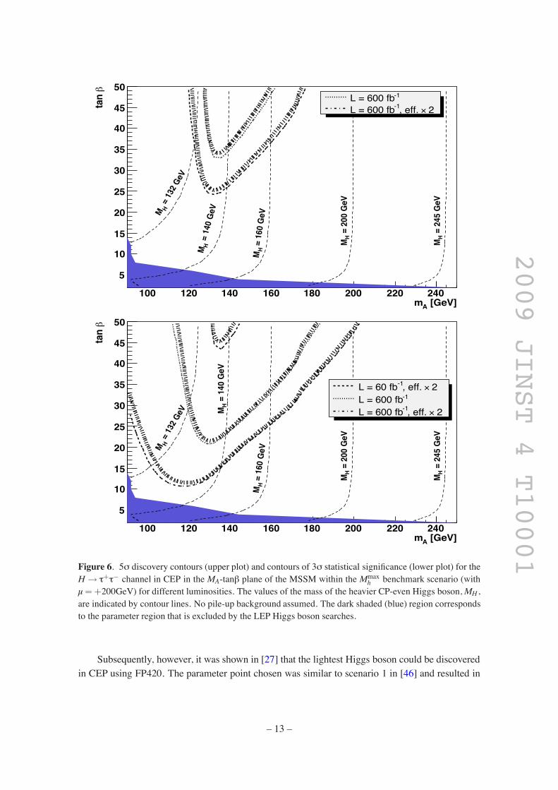
Figure 6 shows the 5σ discovery contours and the 3σ contours in the MA$ tanβ plane for theMmaxh benchmark scenario for different luminosity scenarios. The discovery region is significantly
smaller than for the bb case, although the decay channel can be observed at 3σ across a largearea of parameter space. This would be an important complementary measurement to the standardsearch channels, affording a direct measurement of the quantum numbers of the H . Furthermore,in this region of parameter space, the A is very close in mass to the H and, since the A is heavilysuppressed in CEP, a clean high-precision measurement of the H mass in the ττ channel will bepossible using forward proton tagging. Heinemeyer et al. [19] also investigated the coverage forthe di-tau decay channel of the light h, and found that a 3σ observation could be made in the regiontanβ + 15, Mh < 130GeV/c2 at high luminosity.
2.5 Observation of Higgs bosons in the NMSSM
The Next-to-Minimal Supersymmetric Standard Model (NMSSM) extends the MSSM by the in-clusion of a singlet superfield, S [44]. This provides a natural solution to the µ problem through theλSHuHd superpotential term when the scalar component of S acquires a vacuum expectation value.The Higgs sector of the NMSSM contains three CP-even and two CP-odd neutral Higgs bosons,and a charged Higgs boson. According to [45] the part of parameter space that has no fine-tuningproblems results in the lightest scalar Higgs boson decaying predominantly via h" aa, where a isthe lightest pseudo-scalar. The scalar Higgs boson has a mass of #100GeV/c2. If the a has a massof 2mτ !ma ! 2mb, which is in fact preferred, then the decay channel h" aa" 4τ would becomethe dominant decay chain. This is not excluded by LEP data. In such a scenario the LHC could failto discover any of the Higgs bosons [45].
– 12 –
2009 JINST 4 T10001
[GeV]Am100 120 140 160 180 200 220 240
βta
n
5
10
15
20
25
30
35
40
45
50
= 13
2 GeV
HM
= 1
60 G
eVH
M
= 1
40 G
eV
HM
= 2
00 G
eVH
M
= 2
45 G
eVH
M
-1L = 600 fb 2 ×, eff. -1L = 600 fb
[GeV]Am100 120 140 160 180 200 220 240
βta
n
5
10
15
20
25
30
35
40
45
50
= 13
2 GeV
HM
= 1
60 G
eVH
M
= 1
40 G
eVH
M
= 2
00 G
eVH
M
= 2
45 G
eVH
M
2 ×, eff. -1L = 60 fb -1L = 600 fb
2 ×, eff. -1L = 600 fb
Figure 6. 5σ discovery contours (upper plot) and contours of 3σ statistical significance (lower plot) for theH " τ+τ$ channel in CEP in the MA-tanβ plane of the MSSM within the Mmax
h benchmark scenario (withµ= +200GeV) for different luminosities. The values of the mass of the heavier CP-even Higgs boson,MH ,are indicated by contour lines. No pile-up background assumed. The dark shaded (blue) region correspondsto the parameter region that is excluded by the LEP Higgs boson searches.
Subsequently, however, it was shown in [27] that the lightest Higgs boson could be discoveredin CEP using FP420. The parameter point chosen was similar to scenario 1 in [46] and resulted in
– 13 –

2009 JINST 4 T10001
)-1 s-2 cm33L (x102 4 6 8 10
Sign
ifica
nce
(3 y
ears
)
3
4
5
6
7
8
9MU10MU15MU10 (2ps)
(a)
M (GeV)0 2 4 6 8 10 12 14 16 18 20N
umbe
r of p
seud
o-sc
alar
mea
sure
men
ts
0
1
2
3
4
5
6
7
8
(b)
Figure 7. (a) The significance of observation of h" aa" 4τ using a muon pT trigger threshold of 10GeV/c(or 15GeV/c) for three years of data taking at ATLAS and CMS. Also shown is the increase in the signif-icance due to a factor of five improvement in background rejection from a 2 ps proton time-of-flight mea-surement, see sections 3 and 10, or a comparable gain across all of the rejection variables [27]. (b) A typicala mass measurement for 150 fb$1 of data.
Mh = 92.9GeV/c2 and ma = 9.7GeV/c2, with BR(h" aa) = 92% and BR(a" ττ) = 81%. Theanalysis uses mainly tracking information to define the 4τ final state and triggers on a single muonwith a transverse momentum greater than 10GeV/c, although the analysis still works for an in-creased muon threshold of 15GeV/c. The final event rates are low, approximately 3-4 events afterall cuts at ATLAS or CMS over three years of data taking if the instantaneous luminosity is greaterthan 1033 cm$2 s$1. There is however no appreciable background. Figure 7(a) shows the combinedsignificance of observation at ATLAS and CMS after three years of data taking at a specific instan-taneous luminosity. The mass of the h is obtained using FP420 to an accuracy of 2$ 3GeV/c2
(per event). Furthermore, using FP420 and the tracking information from the central detector, itis possible to make measurements of the a mass on an event-by-event basis. This is shown in fig-ure 7(b) for an example pseudo-data set corresponding to 150 fb$1 of integrated luminosity. Fromexamining many such pseudo-data sets, the mass of the a in this scenario would be measured as9.3±2.3GeV/c2.
A complementary, independent trigger study has also been performed for this decay channelusing the CMS fast simulation. Using only the standard CMS single muon trigger of 14GeV/c, atrigger efficiency of 13% for the h" aa" 4τ was observed. This is in reasonably good agreementwith the study presented above, which observed a 12% efficiency for a 15GeV/c trigger (assumingATLAS efficiencies). Furthermore, the study also observed that the analysis presented above wouldbenefit from additional triggers, which were not considered in [27]. The total trigger efficiency in-creases to #28% if a combination of lepton triggers are used. It is likely that the majority of theseevents will pass the analysis cuts presented in [27] and so would boost the event rate by up to afactor of two. If the lepton trigger thresholds can be reduced, which could be possible at low lumi-nosities, the trigger efficiency increases to 45% resulting in a factor of 3.5 increase in the event rate.
– 14 –

2009 JINST 4 T10001
2.6 Invisible Higgs boson decay modes
In some extensions of the SM, the Higgs boson decays dominantly into particles which cannot bedirectly detected, the so called invisible Higgs. The prospects of observing such Higgs boson viathe forward proton mode are quite promising [47] assuming that the overlap backgrounds can bekept under control. Note that contrary to the conventional parton-parton inelastic production, themass of such invisible Higgs boson can be accurately measured by the missing mass method.
2.7 Conclusion of the studies of the CEP of h,H
It is a general feature of extended Higgs sectors that the heavy Higgs bosons decouple from thegauge bosons and therefore decay predominantly to heavy SM fermions. Adding the possibility todetect the bb decay channel and enhancing the capacity to detect the ττ channel would therefore beof enormous value. In the Mmax
h scenario of the MSSM, if forward proton detectors are installedat 420 m and 220 m and operated at all luminosities, then nearly the whole of the MA$ tanβ planecan be covered at the 3σ level. Even with only 60 fb$1 of luminosity the large tanβ / small MAregion can be probed. For the heavy CP-even MSSM Higgs boson with a mass of approximately140 GeV/c2, observation should be guaranteed for all values of tanβ with sufficient integrated lumi-nosity. At high tanβ, Higgs bosons of masses up to # 240GeV/c2 should be observed with 220 mproton taggers. The coverage and significance are further enhanced for negative values of the µparameter. For scenarios in which the light (heavy) Higgs boson and the A boson are nearly de-generate in mass, FP420 (together with the 220 proton tagger) will allow for a clean separation ofthe states since the A cannot be produced in central exclusive production. In the NMSSM, forwardproton tagging could become the discovery channel in the area of parameter space in which thereare no fine-tuning issues through the decay chain h" aa" 4τ. Using the information from FP420,the mass of both the h and a can be obtained on an event-by-event basis.
Observation of any Higgs state in CEP allows for direct observation of its quantum numbersand a high-precision mass measurement. As we shall see in section 3, it will be possible in manyscenarios to measure the mass with a precision of better than 1GeV/c2 and a width measurementmay also be possible. Installation of FP420 would therefore provide a significant enhancement inthe discovery potential of the current baseline LHC detectors.
2.8 Photon-photon and photon-proton physics
2.8.1 Introduction
Photon-induced interactions have been extensively studied in electron-proton and electron-positroncollisions at HERA and LEP, respectively.
A significant fraction of pp collisions at the LHC will also involve quasi-real (low-Q2) photoninteractions, occurring for the first time at centre-of-mass energies well beyond the electroweakscale. The LHC will thus offer a unique possibility for novel research — complementary to thestandard parton-parton interactions — via photon-photon and photon-proton processes in a com-pletely unexplored regime. The much larger effective luminosity available in parton-parton scat-terings will be compensated by the better known initial conditions and much simpler final statesin photon-induced interactions. The distinct experimental signatures of events involving photonexchanges are the presence of very forward scattered protons and of large rapidity gaps (LRGs)
– 15 –
2009 JINST 4 T10001
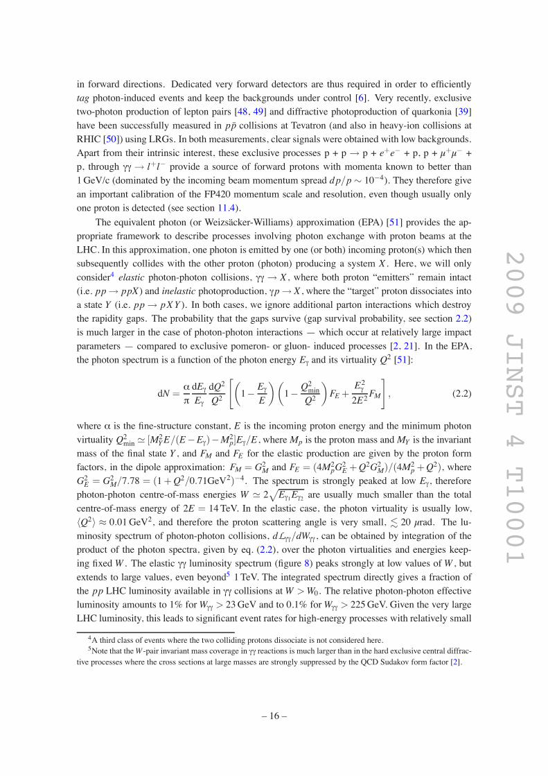
in forward directions. Dedicated very forward detectors are thus required in order to efficientlytag photon-induced events and keep the backgrounds under control [6]. Very recently, exclusivetwo-photon production of lepton pairs [48, 49] and diffractive photoproduction of quarkonia [39]have been successfully measured in pp collisions at Tevatron (and also in heavy-ion collisions atRHIC [50]) using LRGs. In both measurements, clear signals were obtained with low backgrounds.Apart from their intrinsic interest, these exclusive processes p + p " p + e+e$ + p, p + µ+µ$ +p, through γγ " l+l$ provide a source of forward protons with momenta known to better than1GeV/c (dominated by the incoming beam momentum spread dp/p # 10$4). They therefore givean important calibration of the FP420 momentum scale and resolution, even though usually onlyone proton is detected (see section 11.4).
The equivalent photon (or Weizsacker-Williams) approximation (EPA) [51] provides the ap-propriate framework to describe processes involving photon exchange with proton beams at theLHC. In this approximation, one photon is emitted by one (or both) incoming proton(s) which thensubsequently collides with the other proton (photon) producing a system X . Here, we will onlyconsider4 elastic photon-photon collisions, γγ " X , where both proton “emitters” remain intact(i.e. pp" ppX ) and inelastic photoproduction, γp" X , where the “target” proton dissociates intoa state Y (i.e. pp" pXY ). In both cases, we ignore additional parton interactions which destroythe rapidity gaps. The probability that the gaps survive (gap survival probability, see section 2.2)is much larger in the case of photon-photon interactions — which occur at relatively large impactparameters — compared to exclusive pomeron- or gluon- induced processes [2, 21]. In the EPA,the photon spectrum is a function of the photon energy Eγ and its virtuality Q2 [51]:
dN =απdEγEγdQ2
Q2
!
"
1$EγE
#"
1$Q2minQ2
#
FE +E2γ2E2
FM
$
, (2.2)
where α is the fine-structure constant, E is the incoming proton energy and the minimum photonvirtuality Q2min ' [M2
YE/(E$Eγ)$M2p]Eγ/E , whereMp is the proton mass andMY is the invariant
mass of the final state Y , and FM and FE for the elastic production are given by the proton formfactors, in the dipole approximation: FM = G2M and FE = (4M2
pG2E +Q2G2M)/(4M2p +Q2), where
G2E = G2M/7.78 = (1+Q2/0.71GeV2)$4. The spectrum is strongly peaked at low Eγ, thereforephoton-photon centre-of-mass energies W ' 2
%
Eγ1Eγ2 are usually much smaller than the totalcentre-of-mass energy of 2E = 14 TeV. In the elastic case, the photon virtuality is usually low,,Q2- . 0.01GeV2, and therefore the proton scattering angle is very small, ! 20 µrad. The lu-minosity spectrum of photon-photon collisions, dLγγ/dWγγ, can be obtained by integration of theproduct of the photon spectra, given by eq. (2.2), over the photon virtualities and energies keep-ing fixedW . The elastic γγ luminosity spectrum (figure 8) peaks strongly at low values ofW , butextends to large values, even beyond5 1TeV. The integrated spectrum directly gives a fraction ofthe pp LHC luminosity available in γγ collisions atW >W0. The relative photon-photon effectiveluminosity amounts to 1% forWγγ > 23GeV and to 0.1% forWγγ > 225GeV. Given the very largeLHC luminosity, this leads to significant event rates for high-energy processes with relatively small
4A third class of events where the two colliding protons dissociate is not considered here.5Note that theW -pair invariant mass coverage in γγ reactions is much larger than in the hard exclusive central diffrac-
tive processes where the cross sections at large masses are strongly suppressed by the QCD Sudakov form factor [2].
– 16 –

2009 JINST 4 T10001
[ GeV ]γγW0 200 400 600 800 1000
]-1
[ G
eVγγ
dWγγ
dL
-710
-610
-510
-410 total luminosity
with double tag VFDs
Figure 8. Relative elastic luminosity spectrum of photon-photon collisions at the LHC in the range Q2min <Q2 < 2GeV2 (solid blue line) compared to the corresponding luminosity if the energy of each photon isrestricted to the forward detector (VFD) tagging range 20GeV < Eγ < 900GeV (dashed green curve) [12].
photon-photon cross-sections. This is even more true for γp interactions, where both energy reachand effective luminosities are much higher than for the γγ case. Finally, photon physics can be stud-ied also in ion collisions at the LHC [52], where the lower ion luminosities are largely compensatedby the high photon fluxes due to the Z2 enhancement (for each nucleus), where Z is the ion charge.
In this section, we will consider the following exclusive photon-induced processes accessibleto measurement at the LHC with very forward proton tags:
1. two-photon production of lepton pairs (an excellent LHC “luminometer” process),
2. two-photon production of W and Z pairs (as a means to investigate anomalous triple andquartic gauge couplings),
3. two-photon production of supersymmetric pairs,
4. associatedWH photoproduction, and
5. anomalous single top photoproduction.
Realistic studies of all these processes — computed with dedicated packages (MADGRAPH / MADE-VENT [53], CALCHEP [54], LPAIR [55]) including typical ATLAS/CMS acceptance cuts and amodified version of the Pythia generator [56] for all processes involving final-state partons — arediscussed in detail in a recent review on photon-induced interactions at the LHC [12]. A summaryof this work is presented in the following subsections.
2.8.2 Two-photon processes
Elastic two photon interactions yield very clean event topologies at the LHC: two very forward pro-tons measured far away from the IP plus some centrally produced system. In addition, the photonmomenta can be precisely measured using the forward proton taggers, allowing the reconstruction
– 17 –

2009 JINST 4 T10001
Table 1. Production cross sections for pp" ppX (via γγ exchange) for various processes (F for fermion, Sfor scalar) computed with various generators [12].
Processes σ (fb) Generatorγγ" µ+µ$ (pµT > 2 GeV/c, |ηµ| <3.1) 72 500 LPAIR [55]
W+W$ 108.5 MG/ME [53]F+F$ (M = 100 GeV/c2) 4.06 //
F+F$ (M = 200 GeV/c2) 0.40 //
S+S$ (M = 100 GeV/c2) 0.68 //
S+S$ (M = 200 GeV/c2) 0.07 //
H " bb (M = 120 GeV/c2) 0.15 MG/ME [53]
[GeV]0w0 200 400 600 800 1000
[fb]
σ
-210
-110
1
10
210
310-µ+µ→γγ
-W+W→γγ
(m=100 GeV)-F+F→γγ (m=200 GeV)-F+F→γγ
(m=100 GeV)-S+S→γγ
(m=200 GeV)-S+S→γγ
Figure 9. Cross sections for various γγ processes at the LHC as a function of the minimal γγ centre-of-massenergyW0 [12].
of the event kinematics. To illustrate the photon physics potential of the LHC, various pair pro-duction cross sections in two-photon collisions have been computed using a modified version [12]of MADGRAPH/MADEVENT [53]. The corresponding production cross sections are summarised intable 1. Since the cross sections for pair production depend only on charge, spin and mass of theproduced particles, the results are shown for charged and colourless fermions and scalars of twodifferent masses. These cross sections are shown as a function of the minimal γγ centre-of-massenergyW0 in figure 9.
Clearly, interesting γγ exclusive cross sections at the LHC are accessible to measurement. In
– 18 –

2009 JINST 4 T10001
Table 2. Cross sections for pp(γγ" µµ)pp after application of typical ATLAS/CMS muon acceptance cuts,and coincident requirement of a forward proton [12].
cross section [fb] σacc σacc (with forward proton tag)pµT > 3 GeV/c, |ηµ| < 2.5 21 600 1 340pµT > 10 GeV/c, |ηµ| < 2.5 7 260 1 270
particular, the high expected statistics for exclusive W pair production should allow for precisemeasurements of the γγWW quartic couplings. The production of new massive charged particlessuch as supersymmetric pairs [57], is also an intriguing possibility. Similarly, the exclusive pro-duction of the Higgs boson — which has a low SM cross section [58] — could become interestingin the case of an enhanced Hγγ coupling. Last but not least, the two-photon exclusive productionof muon pairs will provide an excellent calibration of luminosity monitors [6, 59].
Lepton pairs. Two-photon exclusive production of muon pairs has a well known QED cross sec-tion, including very small hadronic corrections [60]. Small theoretical uncertainties and a largecross section at LHC energies (σ = 72.5 pb, table 1) makes this process a perfect candidate forthe measurement of the LHC absolute luminosity [6]. Thanks to its distinct signature the selectionprocedure is very simple: two muons within the central detector acceptance (|η|< 2.5), with trans-verse momenta above two possible thresholds (pµT > 3 or 10 GeV/c), and no other charged particleson the dimuon vertex. As the forward protons have very low pT , the muons have equal and op-posite (in φ) momenta. The effective cross sections after the application of these acceptance cuts(σacc), with or without the requirement of at least one FP420 tag, are presented in table 2. About800 muon pairs should be detected in 12 hour run at the average luminosity of 1033 cm$2s$1.
An important application of these exclusive events is the absolute calibration of the very for-ward proton detectors. As the energy of the produced muons is well measured in the central de-tector, the forward proton energy can be precisely predicted using the kinematics constraints. Thisallows for precise calibration of the proton taggers, both momentum scale and resolution, in case ofe.g. misalignment of the LHC beam-line elements, and leads to a good control of the reconstructedenergy of the exchanged photon [61]. The large cross sections could even allow for run-by-runcalibration, as the requirement of at least one forward proton tag results in more than 300 eventsper run. As the momenta of both forward protons are known from the central leptons, it is onlynecessary to measure one of them. This is fortunate as it allows low mass (#10 GeV/c2) forwardpairs to be used, with rates much higher than in the FP420 double-arm acceptance. Finally, it isworth noting that the two-photon exclusive production of e+e$ pairs can also be studied at theLHC, though triggering of such events is more difficult. Electron pair reconstruction, e.g. in theCMS CASTOR forward calorimeter, has been discussed in [8].
W and Z boson pairs. A large cross section of about 100 fb is expected for the exclusive two-photon production ofW boson pairs at the LHC. The very clean event signatures offer the possibil-ity to study the properties of theW gauge bosons and to make stringent tests of the Standard Modelat average centre-of-mass energies of
&
Wγγ"WW'
. 500GeV. The cross section for events where
– 19 –
2009 JINST 4 T10001
Table 3. Cross section σacc for γγ"W+W$ " µ+µ$νµνµ after application of typical ATLAS/CMS muonacceptance cuts, and coincident requirement of a forward proton [12].
cross section [fb] σacc σacc (with forward proton tag)pµT > 3 GeV/c, |ηµ| < 2.5 0.80 0.76pµT > 10 GeV/c, |ηµ| < 2.5 0.70 0.66
bothW bosons decay into a muon and a neutrino — resulting in events with only two muons withlarge transverse momentum within the typical |η| < 2.5 ATLAS/CMS muon acceptance range —are large and only slightly reduced after adding the requirement of at least one forward proton tag(table 3).
The unique signature ofWW pairs in the fully leptonic final state, no additional tracks on thel+l$ vertex, large lepton acoplanarity and large missing transverse momentum strongly reduces thebackgrounds. The two-photon production of tau-lepton pairs, having in addition a low cross-sectionat large invariant masses, can then be completely neglected. Moreover, the double diffractive pro-duction of theW boson pairs is also negligible, and the inclusive partonic production (about 1 pb,assuming fully leptonic decays, and both leptons passing the acceptance cuts) can be very effi-ciently suppressed too by applying either the double tagging in the forward proton detectors, orthe double LRG signature. Similar conclusions can be reached for the exclusive two-photon pro-duction of Z boson pairs, assuming fully leptonic, or semi-leptonic decays. In the SM, γγ" ZZ isnegligible; this would be a test of anomalous γZZ couplings. The dominant SM source of exclusiveZZ is H " ZZ if the Higgs boson exists, so the background in this channel is very small.
Two-photon production of W pairs provides a unique opportunity to investigate anomalousgauge boson couplings, in particular the quartic gauge couplings (QGCs), γγWW [62]. The sensi-tivity to the anomalous quartic vector boson couplings has been investigated [12] in the processesγγ"W+W$ " l+l$νν and γγ" ZZ" l+l$ j j using the signature of two leptons (e or µ) withinthe acceptance cuts |η| < 2.5 and pT > 10 GeV/c. The upper limits λup on the number of events atthe 95% confidence level have been calculated assuming that the number of observed events equalsthat of the SM prediction (corresponding to all anomalous couplings equal to zero). The calculatedcross section upper limits can then be converted to one-parameter limits (when the other anoma-lous coupling is set to zero) on the anomalous quartic couplings. The obtained limits (table 4) areabout 4000 times better than the best limits established at LEP2 [63] clearly showing the large andunique potential of such studies at the LHC. A corresponding study of the anomalous triple gaugecouplings can also be performed [64]. However, in this case the expected sensitivities are not asfavourable as for the anomalous QGCs.
Supersymmetric pairs. The interest in the two-photon exclusive production of pairs of newcharged particles is three-fold: (i) it provides a new and very simple production mechanism forphysics beyond the SM, complementary to the standard parton-parton processes; (ii) it can signifi-cantly constrain the masses of the new particles, using double forward-proton tagging information;(iii) in the case of SUSY pairs, simple final states are usually produced without cascade decays,characterised by a fully leptonic final state composed of two charged leptons with large missing en-
– 20 –

2009 JINST 4 T10001
Table 4. Expected one-parameter limits for anomalous quartic vector boson couplings at 95% CL [12].
Coupling limitsR
Ldt= 1fb$1R
Ldt= 10fb$1
[10$6 GeV$2 ]
|aZ0/Λ2| 0.49 0.16|aZC/Λ2| 1.84 0.58|aW0 /Λ2| 0.54 0.27|aWC /Λ2| 2.02 0.99
Figure 10. Relevant Feynman diagrams for SUSY pair production with leptons in the final state: charginodisintegration in a charged/neutral scalar and a neutral/charged fermion (left); slepton disintegration(right) [12].
ergy (and large lepton acoplanarity) with low backgrounds, and large high-level-trigger efficiencies.The two-photon production of supersymmetric leptons or other heavy non-Standard Model
leptons has been investigated in [57, 65–67]. The total cross-section at the LHC for the processγγ" l+ l$ can be as large as# 20 fb (O(1 f b) for the elastic case alone), while still being consistentwith the model-dependent direct search limits from LEP [68, 69]. While sleptons are also producedin other processes (Drell-Yan or squark/gluino decays), γγ production has the advantage of being adirect QED process with minimal theoretical uncertainties.
In [12], three benchmark points in mSUGRA/CMSSM parameter space constrained by thepost-WMAP research [70] have been chosen:
• LM1: very light LSP, light !, light χ and tanβ=10;
• LM2: medium LSP, heavy !, heavy χ and tanβ=35;
• LM6: heaviest LSP, light right !, heavy left !, heavy χ and tanβ=10.
The masses of the corresponding supersymmetric particles are listed in table 5.The study concentrates on the fully leptonic SUSY case only. The corresponding Feynman
diagrams are shown in figure 10. Signal and background samples coming from SUSY and SMpairs were produced using a modified version of CALCHEP [54]. The following acceptance cutshave been applied: two leptons with pT > 3 GeV/c or 10 GeV/c and |η|< 2.5. The only irreducible
– 21 –

2009 JINST 4 T10001
Table 5. Masses of SUSY particles, in GeV/c2, for different benchmarks (here ! = e,µ).
m [GeV/c2] LM1 LM2 LM6χ01 97 141 162!+R 118 229 175
!+L 184 301 283τ+1 109 156 168τ+2 189 313 286χ+1 180 265 303χ+2 369 474 541
H+ 386 431 589
background for this type of processes is the exclusive W pair production since direct lepton pairspp(γγ " !+!$)pp can be suppressed by applying large acoplanarity cuts. Standard high-level-trigger (HLT) efficiencies are high for all these types of events. In typical mSUGRA/CMSSMscenarios, a light right-handed slepton will have a branching fraction of B(l± " χ01l±) = 100%.This results in a final state with two same-flavor opposite-sign leptons, missing energy, and twooff-energy forward protons. Assuming a trigger threshold of 7 GeV/c for two isolated muons,the efficiency would be 71$ 74% for smuons in the range of typical light mSUGRA/CMSSMbenchmark points (LM1 or SPS1a). With an integrated luminosity of 100 fb$1, this would resultin a sample of 15$ 30 triggered elastic-elastic smuon pairs, plus a slightly smaller number ofselectron pairs. Including the less clean singly-elastic events would increase these yields by roughlya factor of 5. The irreducible γγ "WW background can be suppressed by a factor of two byselecting only same lepton-flavour (ee, µµ) final states. The measured energy of the two scatteredprotons in forward proton taggers could allow for the distinction between various contributions tothe signal by looking at the distribution of the photon-photon invariant massWγγ. HECTOR [61]simulations of forward protons from slepton events consistent with LM1 benchmark point indicatethat the TOTEM 220 m detectors will have both protons tagged for only 30% of events. Additionof detectors at 420 m increases that to 90% of events.
The expected cumulativeWγγ distributions for LM1 events with two centrally measured leptonsand two forward detected protons are illustrated in figure 11. With this technique and sufficientstatistics, masses of supersymmetric particles could be measured with precision of a few GeV/c2 bylooking at the minimal centre-of-mass energy required to produce a pair of SUSY particles. In thesame way, missing energy can be computed by subtracting the detected lepton energies from themeasured two-photon centre-of-mass energy. For backgrounds missing energy distributions startat zero missing energy, while in SUSY cases they start only at two times the mass of the LSP.
2.8.3 Photon-proton processes
The high luminosity and the high centre-of-mass energies of photo-production processes at theLHC offer very interesting possibilities for the study of electroweak interaction and for searchesBeyond the Standard Model (BSM) up to the TeV scale [12]. Differential cross sections for
– 22 –

2009 JINST 4 T10001
µµLM1: ee/
[GeV]γγW0 200 400 600 800 1000 1200
# ev
ents
/ 15
GeV
0
1
2
3
4
5
6µµLM1: ee/
) / 3-W+ W→ γγ(
-Rµ∼+
Rµ∼, -
Re~+R
e~ → γγ
-Lµ∼
+Lµ∼, -
Le~+L
e~ → γγ
-2χ∼
+2χ∼, -
1χ∼
+1χ∼ → γγ
-2τ∼+
2τ∼, -
1τ∼+
1τ∼ → γγ
-1L = 100 fb# events = 69.47
eµ/µLM1: e
[GeV]γγW0 200 400 600 800 1000 1200
# ev
ents
/ 50
GeV
0
0.2
0.4
0.6
0.8
1eµ/µLM1: e
) / 60-W+ W→ γγ(
-2χ∼
+2χ∼, -
1χ∼
+1χ∼ → γγ
-Lµ∼
+Lµ∼, -
Le~+L
e~ → γγ
-2τ∼+
2τ∼, -
1τ∼+
1τ∼ → γγ
-1 L = 100 fb# events = 5.262
Figure 11. Photon-photon invariant mass for benchmark point LM1 withR
Ldt = 100 fb$1. Cumulativedistributions for signal with two detected leptons (pT > 3 GeV/c, |η|< 2.5), two detected protons, with same(left) or different flavour (right). TheWW background has been down-scaled by the quoted factor [12].
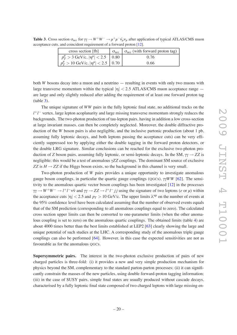
pp(γq/g " X)pY reactions, as a function of the photon-proton centre-of-mass energy, are pre-sented in figure 12 together with the acceptance region of forward proton taggers. A large varietyof processes have sizeable cross section up to the electroweak scale and could therefore be studiedduring the very low and low luminosity phases of the LHC. Interestingly, potential Standard Modelbackground processes with hard leptons, missing energy and jets coming from the production ofgauge bosons, have cross sections only one or two orders of magnitude higher than those involvingtop quarks. The large top quark photo-production cross sections, O(pb), are particularly interestingfor measuring top quark related SM parameters, such as the top quark mass and its electric charge.In addition, and in contrast to parton-parton top production, photo-production of top quark pairsand of single top in association with a W boson have similar cross sections. This will certainlybe advantageous in analyses aiming at measuring the Cabibbo-Kobayashi-Maskawa (CKM) matrixelement |Vtb| in associatedWt production.
In order to illustrate the discovery potential of photon-proton interactions at the LHC, wediscuss in the next two subsections the possibility to observe: (i) the SM Higgs boson produced inassociation with aW (σWH . 20 fb for MH = 115 GeV/c2, representing more than 2% of the totalinclusive WH production at the LHC), (ii) the anomalous production of single top, which couldreveal BSM phenomena via Flavour Changing Neutral Currents (FCNC).
Associated WH production. The search forWH associate production at the LHC will be chal-lenging due to the largeW+jets, tt andWZ cross sections. Indeed, although Standard Model crosssections for the partonic process pp" (qq) "WHX range from 1.5 pb to 425 fb for Higgs bosonmasses of 115 GeV/c2 and 170 GeV/c2 respectively, this reaction is generally not considered asa Higgs discovery channel. This production mechanism however, is sensitive to WWH couplingwhich might be enhanced when considering fermiophobic models, and might also give valuableinformation on the Hbb coupling, which is particularly difficult to determine at the LHC. The pos-sibility of using γp collisions to search for WH associate production was already considered atelectron-proton colliders [71]. At the LHC the cross section for pp" (γq) "WHq( pY reactionreaches 23 (17.5) fb for a Higgs boson mass of 115 GeV/c2 (170 GeV/c2). The dominant Feynmandiagrams are shown in figure 13. Although cross sections are smaller than the ones initiated by
– 23 –
2009 JINST 4 T10001
[GeV] pγw0 2000 4000 6000 8000 10000 12000
[fb/
GeV]
pγdwσd
-410
-310
-210
-110
1
10
210
VFD 220 - 2 mm
VFD 420 - 4 mm
Wj→qγjγ→qγ
Zj→qγtt→gγ
Wt→qγq’-W+W→qγ
WZq’→qγ=115 GeV)
HWHq’ (m→qγWWWq’→qγ
Figure 12. Differential cross-sections for pp(γq/g" X)pY processes as a function of the c.m.s. energy inphoton-proton collisions,Wγp. The acceptance of roman pots (220 m at 2 mm from the beam axis and 420 mat 4 mm from the beam axis) is also sketched [12].
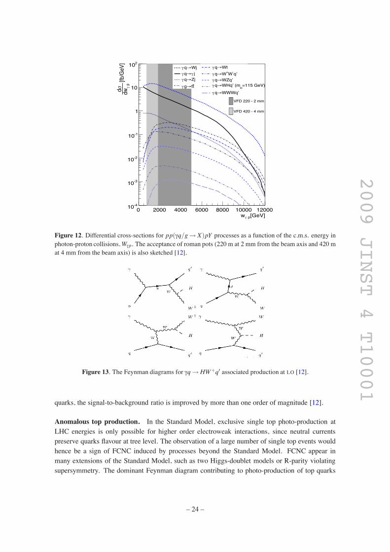
Figure 13. The Feynman diagrams for γq" HW+q( associated production at LO [12].
quarks, the signal-to-background ratio is improved by more than one order of magnitude [12].
Anomalous top production. In the Standard Model, exclusive single top photo-production atLHC energies is only possible for higher order electroweak interactions, since neutral currentspreserve quarks flavour at tree level. The observation of a large number of single top events wouldhence be a sign of FCNC induced by processes beyond the Standard Model. FCNC appear inmany extensions of the Standard Model, such as two Higgs-doublet models or R-parity violatingsupersymmetry. The dominant Feynman diagram contributing to photo-production of top quarks
– 24 –

2009 JINST 4 T10001
Figure 14. Photo-production of top quarks at LHC through FCNC [12].
Table 6. Expected limits for anomalous couplings at 95% CL [12].
Coupling limitsR
Ldt = 1 fb$1R
Ldt = 10 fb$1
ktuγ 0.043 0.024ktcγ 0.074 0.042
via FCNC, can be seen in figure 14. The effective Lagrangian for this anomalous coupling can bewritten as [72]:
L= ieet tσµνqν
ΛktuγuAµ+ ieet t
σµνqν
ΛktcγcAµ+h.c.,
where σµν is defined as (γµγν$ γνγµ)/2, qν being the photon 4-vector and Λ an arbitrary scale,conventionally taken as the top mass. The couplings ktuγ and ktcγ are real and positive such that thecross section takes the form:
σpp"t = αu k2tuγ +αc k2tcγ.
The computed α parameters using CALCHEP are αu = 368 pb,αc = 122 pb. The best limit on ktuγis around 0.14, depending on the top mass [73] while the anomalous coupling ktcγ has not beenprobed yet.
The single top final state is composed of a b-jet and aW boson. The main irreducible back-grounds for the considered topology, !EmissT b, come from γp interactions producing aW boson anda jet, especially c-jets which can be miss-tagged as a b-jets. Limits on the anomalous couplingsktuγ and ktcγ have been extracted after application of acceptance cuts in [12]. These results appearon table 6 for two integrated luminosities.
2.8.4 Photon-photon and photon-proton physics summary
A summary of various unique photon-photon and photon-proton interactions accessible to mea-surement at the LHC, and discussed in detail in [12], has been presented in this section. Interestingstudies and searches can be performed for initial integrated luminosities of about 1 fb$1, such asexclusive dimuon production in two-photon collisions tagged with forward large rapidity gaps. Athigher luminosities, the efficient selection of photon-induced processes is greatly enhanced withdedicated forward proton taggers such as FP420. Photon induced reactions can provide muchhigher sensitivity than partonic reactions for various BSM signals such as e.g. anomalous quar-tic γγWW gauge couplings. The associated photoproduction of a top quark or aW boson is also
– 25 –

2009 JINST 4 T10001
very large, offering a unique opportunity to measure the fundamental Standard Model parameters,such as the top quark charge or the Vtb element of the quark mixing matrix. Anomalous γqt cou-plings might also be uniquely revealed in single top photoproduction. Larger integrated luminosity,of about hundred inverse femtobarns, will open complementary ways to search for production ofsupersymmetric particles in photon-photon interactions. Even larger luminosities might help toaccess important information on the Higgs boson coupling to b quarks andW bosons. FP420 de-tectors are mandatory for the determination of the masses of the centrally produced particles, andto increase the sensitivity to new anomalous couplings contributions in two-photon interactions.
Last but not least, studying the photon-induced processes in the early LHC runs can pro-vide valuable checks of the various components of the general formalism used to predict the crosssections of central exclusive reactions [36]. Thus, the photon-exchange dominated W -boson pro-duction with rapidity gaps on either side provides information on the gap survival factor S2. Asdiscussed in [36], such studies can be performed even without tagging of the forward proton. An-other example is exclusive ϒ photoproduction induced by the process γp" ϒp [74]. The study ofsuch processes will not only reduce the theoretical uncertainties associated with the generalised,unintegrated gluon distributions fg, e.g., by testing models based on diffusion in transverse mo-mentum as incarnated in the Balitsky-Fadin-Kuraev-Lipatov (BFKL) equation [75], but will be ofhelp to calibrate and align the forward proton detectors.
2.9 Diffractive physics
Proton tagging with FP420 will allow a continuation of the study of hard diffraction, expandingand extending the investigations carried out at CERN by UA8 [76], and more recently at HERAby H1 and ZEUS and at Fermilab by CDF and D0 (see, e.g., [8, 77–79] and references therein).The coverage of FP420, 0.002 < ξ < 0.02, is centred on the diffractive peak region where thecontribution from mesonic exchanges (Reggeons) is negligible, and is thus complementary to thatof TOTEM (or of any near-beam detectors at 220 m from the interaction point), which is 0.02 <
ξ< 0.2 with high luminosity LHC optics (see figure 15).The following reactions can be studied:
1. at instantaneous luminosities where pile-up is negligible, single diffractive (SD) dissociationof the proton, pp" X p, where one proton is measured in FP420 and the other dissociatesinto a state X which contains high-ET jets, vector bosons or heavy flavours: the limitation tolow luminosities is due to the fact that the timing constraint cannot be applied when only oneproton is measured;
2. at all luminosities, double pomeron exchange (DPE), pp " pX p, where both protons aretagged by FP420, and again X includes high-ET jets, vector bosons or heavy flavours;
3. also at all luminosities, central exclusive production of di-jets, pp" p j jp.
Processes 1 and 2 are sensitive to the low-x structure of the proton and the diffractive partondistribution functions (dPDFs), which can be interpreted as conditional probabilities to find a partonin the proton when the final state of the process contains a fast proton of given four-momentum.Process 3 is sensitive to the generalised (skewed) parton distribution functions (GPD), which arecrucial for the estimate of the cross section for central exclusive Higgs production.
– 26 –
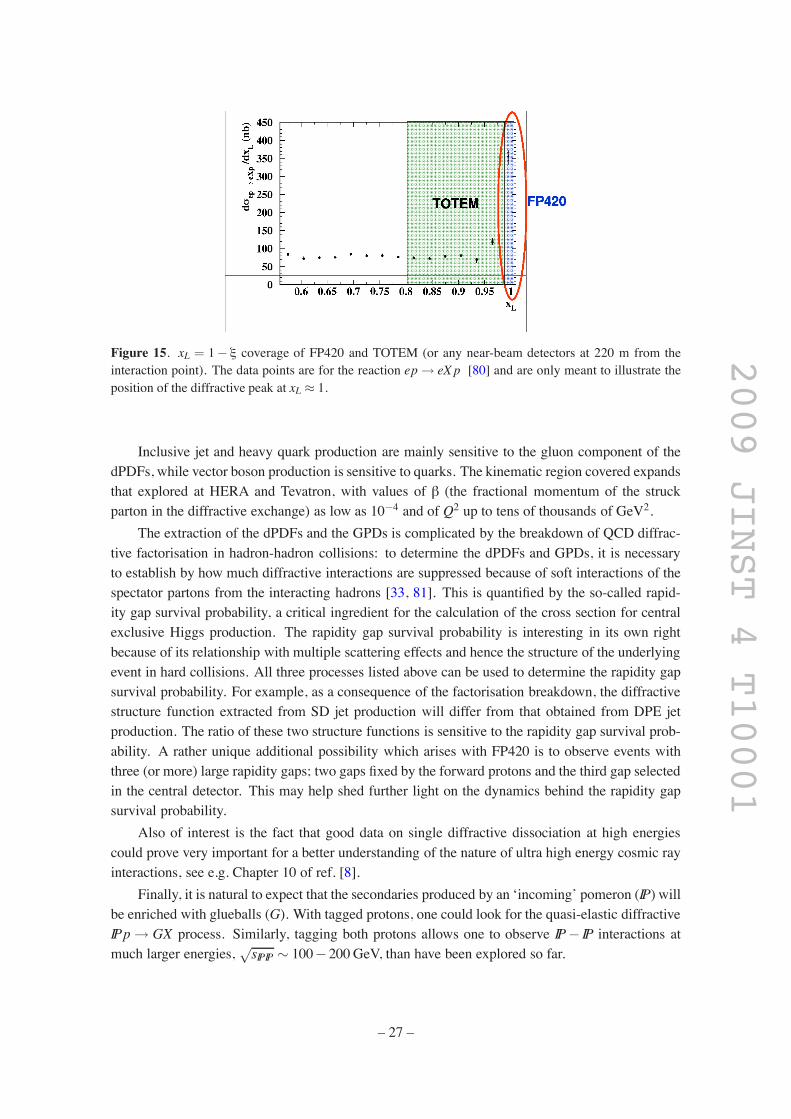
2009 JINST 4 T10001
Figure 15. xL = 1$ ξ coverage of FP420 and TOTEM (or any near-beam detectors at 220 m from theinteraction point). The data points are for the reaction ep" eX p [80] and are only meant to illustrate theposition of the diffractive peak at xL . 1.
Inclusive jet and heavy quark production are mainly sensitive to the gluon component of thedPDFs, while vector boson production is sensitive to quarks. The kinematic region covered expandsthat explored at HERA and Tevatron, with values of β (the fractional momentum of the struckparton in the diffractive exchange) as low as 10$4 and of Q2 up to tens of thousands of GeV2.
The extraction of the dPDFs and the GPDs is complicated by the breakdown of QCD diffrac-tive factorisation in hadron-hadron collisions: to determine the dPDFs and GPDs, it is necessaryto establish by how much diffractive interactions are suppressed because of soft interactions of thespectator partons from the interacting hadrons [33, 81]. This is quantified by the so-called rapid-ity gap survival probability, a critical ingredient for the calculation of the cross section for centralexclusive Higgs production. The rapidity gap survival probability is interesting in its own rightbecause of its relationship with multiple scattering effects and hence the structure of the underlyingevent in hard collisions. All three processes listed above can be used to determine the rapidity gapsurvival probability. For example, as a consequence of the factorisation breakdown, the diffractivestructure function extracted from SD jet production will differ from that obtained from DPE jetproduction. The ratio of these two structure functions is sensitive to the rapidity gap survival prob-ability. A rather unique additional possibility which arises with FP420 is to observe events withthree (or more) large rapidity gaps; two gaps fixed by the forward protons and the third gap selectedin the central detector. This may help shed further light on the dynamics behind the rapidity gapsurvival probability.
Also of interest is the fact that good data on single diffractive dissociation at high energiescould prove very important for a better understanding of the nature of ultra high energy cosmic rayinteractions, see e.g. Chapter 10 of ref. [8].
Finally, it is natural to expect that the secondaries produced by an ‘incoming’ pomeron (IP) willbe enriched with glueballs (G). With tagged protons, one could look for the quasi-elastic diffractiveIPp" GX process. Similarly, tagging both protons allows one to observe IP$ IP interactions atmuch larger energies, )sIPIP # 100$200GeV, than have been explored so far.
– 27 –

2009 JINST 4 T10001
Table 7. Cross sections for a few hard diffractive processes, as obtained with the POMWIG generator [82].
Process Cross sectionpp" X p, with X including aW boson 70 pbpp" X p, with X including a di-jet (ET > 50GeV) 30 nbpp" pX p, with X including a di-jet (ET > 50GeV) 1.5 nb
Cross sections for hard diffractive processes can be large, as shown in table 7. In the following,we summarise some of the studies that have been performed.
2.9.1 Single diffractive production ofW , Z bosons or di-jets
Selection efficiencies were studied in [8, 83] for pp" pX , with X containing a W or a Z bosonthat decays to jets or to muons, as well as with X containing a di-jet system. Samples of 100,000signal events each were generated with the POMWIG Monte Carlo generator [82] (version 1.3).For these studies, the CMS detector response was simulated using the OSCAR [84] package. Thedigitisation (simulation of the electronic response), the emulation of the Level-1 and High-LevelTriggers (HLT), and the offline reconstruction of physics objects were performed with the CMSfull-reconstruction ORCA package [85]. For four example processes, figure 16 shows the efficiencyas a function of the L1 threshold value, normalised to the number of events (in the muon rate caseto the number of events with a muon in the final state) with 0.001< ξ< 0.2. Three different triggerconditions are considered: (i) only central detector information, (ii) central detector information inconjunction with a single arm track at 220 m and (iii) central detector information in conjunctionwith a single arm track at 420 m. Also shown is the number of events expected to pass the L1selection per pb$1 of LHC running. In [8, 83], a gap survival probability of unity was assumed.However, at the LHC this factor is expected to be O(0.1) [86].
2.9.2 Single diffractive and double pomeron exchange production of Bmesons
Inclusive SD and DPE production of B mesons, with B" J/ψX and J/ψ" µ+µ$, was studiedin [8] using the generator DPEMC 2.4 [87] in conjunction with the fast CMS simulation codeFAMOS, version 1.3.1 [88]. As discussed earlier, this process is sensitive to the dPDFs of theproton. Events were selected which had at least one pair of oppositely charged muons. If two pairswere found, the one with invariant mass closer to that of the J/ψ meson was taken to be the oneoriginating from the J/ψ decay. Events were selected if 2.7 < Mµµ < 3.5 GeV/c2, with Mµµ theinvariant mass of the muon pair, pµT > 3 GeV/c (at L1) and pµT > 7 GeV/c (HLT). In addition, thedetection of a proton on either side of the interaction point was required for the SD events and onboth sides for the DPE events. The estimated event yield, after the cuts, for an integrated luminosityof 1 fb$1 is of hundreds of SD events and a few DPE events.
2.9.3 Double pomeron exchange production ofW bosons
Also studied in [8] is inclusive DPE production of W bosons, pp " pXW p, which probes thedPDFs of the proton. The reaction was simulated with the DPEMC generator v2.4 [87]. The
– 28 –
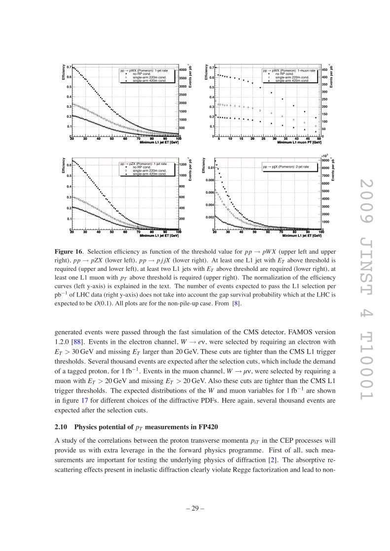
2009 JINST 4 T10001
Minimum L1 jet ET [GeV]20 30 40 50 60 70 80 90 100
Minimum L1 jet ET [GeV]20 30 40 50 60 70 80 90 100
Effic
ienc
y
0
0.1
0.2
0.3
0.4
0.5
0.6
0.7 -1Ev
ents
per
pb
0
500
1000
1500
2000
2500
3000
3500
4000 pWX (Pomeron): 1-jet rate→pp no RP cond.single-arm 220m cond.single-arm 420m cond.
Minimum L1 muon PT [GeV]5 10 15 20 25 30 35 40 45 50
Minimum L1 muon PT [GeV]5 10 15 20 25 30 35 40 45 50
Effic
ienc
y
0
0.1
0.2
0.3
0.4
0.5
0.6
0.7
-1Ev
ents
per
pb
0
50
100
150
200
250
300
350
400
450 pWX (Pomeron): 1-muon rate→pp no RP cond.single-arm 220m cond.single-arm 420m cond.
Minimum L1 jet ET [GeV]20 30 40 50 60 70 80 90 100
Minimum L1 jet ET [GeV]20 30 40 50 60 70 80 90 100
Effic
ienc
y
0
0.1
0.2
0.3
0.4
0.5
0.6
-1Ev
ents
per
pb
0
200
400
600
800
1000
1200 pZX (Pomeron): 1-jet rate→pp no RP cond.single-arm 220m cond.single-arm 420m cond.
Minimum L1 jet ET [GeV]20 30 40 50 60 70 80 90 100
Minimum L1 jet ET [GeV]20 30 40 50 60 70 80 90 100
Effic
ienc
y
0
0.002
0.004
0.006
0.008
0.01
-1Ev
ents
per
pb
0
1000
2000
3000
4000
5000
6000
7000
8000
9000
310×
pjjX (Pomeron): 2-jet rate→pp
Figure 16. Selection efficiency as function of the threshold value for pp " pWX (upper left and upperright), pp" pZX (lower left), pp" p j jX (lower right). At least one L1 jet with ET above threshold isrequired (upper and lower left), at least two L1 jets with ET above threshold are required (lower right), atleast one L1 muon with pT above threshold is required (upper right). The normalization of the efficiencycurves (left y-axis) is explained in the text. The number of events expected to pass the L1 selection perpb$1 of LHC data (right y-axis) does not take into account the gap survival probability which at the LHC isexpected to be O(0.1). All plots are for the non-pile-up case. From [8].
generated events were passed through the fast simulation of the CMS detector, FAMOS version1.2.0 [88]. Events in the electron channel, W " eν, were selected by requiring an electron withET > 30GeV and missing ET larger than 20GeV. These cuts are tighter than the CMS L1 triggerthresholds. Several thousand events are expected after the selection cuts, which include the demandof a tagged proton, for 1 fb$1. Events in the muon channel,W " µν, were selected by requiring amuon with ET > 20GeV and missing ET > 20GeV. Also these cuts are tighter than the CMS L1trigger thresholds. The expected distributions of the W and muon variables for 1 fb$1 are shownin figure 17 for different choices of the diffractive PDFs. Here again, several thousand events areexpected after the selection cuts.
2.10 Physics potential of pT measurements in FP420
A study of the correlations between the proton transverse momenta piT in the CEP processes willprovide us with extra leverage in the the forward physics programme. First of all, such mea-surements are important for testing the underlying physics of diffraction [2]. The absorptive re-scattering effects present in inelastic diffraction clearly violate Regge factorization and lead to non-
– 29 –

2009 JINST 4 T10001
(W) [GeV] TRANSVERSEM20 40 60 80 100 120 140
Even
ts
0
500
1000
1500
2000
2500
(W) [GeV]TP0 10 20 30 40 50 60 70 80 90 100
Even
ts
1
10
210
310
[GeV]TMuon E20 30 40 50 60 70
Even
ts
10
210
310
ηMuon -3 -2 -1 0 1 2 3
Even
ts
0
200
400
600
800
1000
Figure 17. Distributions, forR
Ldt = 1 fb$1, of (a) transverse mass of the W± boson, (b) transverse mo-mentum of the W±, (c) transverse momentum of the muon, (d) pseudorapidity of the muon for W " µν.Full points: approximately flat diffractive gluon density (H1 fit 2 [89]); histograms: more peaked diffractivegluon density (H1 fit 3 [89]). From [8].
trivial correlations between proton transverse momenta p1T and p2T in the process pp" p+M+ p.Measuring the transverse momenta and the azimuthal angle ϕ distribution for different values pit ,allows a detailed probe of the opacity of the incoming proton, and more generally, testing the dy-namics of soft survival. One of the best examples to study such effects is exclusive high ET dijetproduction [2, 37], where the cross section for the hard subprocess is large and well known.
Another important feature of the correlation study is that it offers a unique possibility for directobservation of a CP-violating signal in the Higgs sector by measuring the azimuthal asymmetry ofthe outgoing tagged protons [28, 90]. In some MSSM scenarios the azimuthal asymmetry
A=σ(ϕ< π)$σ(ϕ> π)σ(ϕ< π)+σ(ϕ> π)
(2.3)
is expected [28] to be quite sizable. For instance, A ' 0.07, in a benchmark scenario of maximalCP-violation ([91]) or in the tri-mixing scenario of ref. [26].
– 30 –

2009 JINST 4 T10001
2.11 Other physics topics
2.11.1 Pomeron/graviton duality in AdS/CFT
Another motivation for further study of central exclusive production is as a testing ground of pos-sible connections with string theory, through the so-called Anti-de-Sitter/Conformal-Field-Theory(AdS/CFT) or “gauge/string” correspondence [92]. The application of AdS/CFT correspondencebetween strongly coupled QCD and weakly coupled gravity has recently successfully appliedto the computation of various observables in high energy heavy-ion physics (see e.g. [93] andrefs. therein). Diffractive scattering and the pomeron represent another area where a connectionwith the string-theory-based techniques may well be ripe. Like heavy-ion physics, the physics ofdiffraction and the pomeron lies largely outside the regime where perturbative field theory com-putations can be performed with confidence. Indeed they are known not to fully describe HERAdata. Thus as in heavy-ion physics, there is much interest in approaching these phenomena with atool which replaces non-perturbative field theory with perturbative string theory. The connectionwith the stringy aspects of the five-dimensional description is indeed very direct in the case ofRegge phenomenology.
A number of papers by string theorists and recently even QCD/nuclear theorists have stud-ied aspects of the pomeron, which in the string theory description is related to the graviton andits higher spin partners on the leading (five-dimensional) Regge trajectory (see e.g. [94] and refs.therein). The physics of the pomeron has been described with considerable technical success, al-lowing insights into various aspects of Regge phenomenology in the corresponding four-dimensionalgauge theories. Few attempts have been made so far to connect these technical results with QCDdata, and the question of whether this connection will be as suggestive as in the nucleus-nucleuscase remains open at present. Also, important problems of relevance to the current proposal, suchas central hadron production, rapidity gap suppression, and Higgs boson production are just nowreceiving some (as yet unpublished) technical consideration from theorists. But there is a real op-portunity for growth of an interdisciplinary research area out of diffractive physics in general andcentral diffractive production in particular.
2.11.2 Exotic new physics scenarios in CEP
A.R. White has developed [95, 96] a theory of the pomeron which requires the existence of newparticles in the LHC domain, and would give rise to dramatic effects in diffraction. If correct,exclusive processes such as p+ p" p+W+W$ + p and p+ p" p+ZZ+ p could be orders ofmagnitude higher than in the Standard Model. In the Standard Model, exclusive W+W$ produc-tion occurs mainly through γγ"W+W$ and h"W+W$, if the Higgs boson exists with Mh #135GeV/c2. Exclusive ZZ production only proceeds, to a good approximation, through h decay. InWhite’s theory the pomeron is approximately a reggeised gluon together with a sea of ‘wee’ gluons,with the unitary Critical pomeron produced via reggeon field theory interactions. A special versionof QCD, QCDS, is required in which the asymptotic freedom constraint is saturated, a requirementnaturally satisfied by QCDS, which contains the known six colour triplet quarks plus a doublet,[U,D], of heavy (hundreds of GeV) colour sextet quarks. The Higgs mechanism is provided, notby a fundamental scalar Higgs boson, but by sextet pion composites, i.e. [UU $DD]. This resultsin a relatively strong coupling between the pomeron and vector bosons, with large cross sections
– 31 –

2009 JINST 4 T10001
for IPIP"W+W$ and IPIP" ZZ. The enhancement in diffractiveW+W$ and ZZ production (butnotWZ production) should be large enough to see without forward proton tagging, with or withoutrequiring large rapidity gaps. However, determining that the pomeron - vector boson coupling isresponsible and studying it in detail will require forward proton measurements. QCDS provides anatural dark matter candidate, the sextet neutron, N6 = [UDD], which should be stable and have amass in the TeV range. QCDS also embeds uniquely in an underlying SU(5) theory, called QUD,which potentially describes the full Standard Model.
3 Simulated measurement of h" bb in the MSSM
As a more detailed example of our proposed methodology, we describe in this section how weintend to study the production of the MSSM h" bb channel. Full details can be found in [20].Similar cuts to reduce the backgrounds are found in the analysis for the CMS-TOTEMdocument [8]and also in ref. [19]. There are two properties of FP420 that are critical to the detection of Higgsbosons in any decay channel. The first is the acceptance, described in detail in section 4, whichfor a fixed LHC optics depends primarily on the distance of approach of the active edge of thesilicon detectors to the beam. We will focus on those events in which both protons are taggedat 420 m, although we comment on the inclusion of forward detectors at 220 m in section 3.4.For 120GeV/c2 central systems, the acceptance is independent of the distance of approach out toapproximately 7 mm (10σ is 2.5 mm at 420 m). Here we assume that the active edge of the 420 mdetectors is 5 mm from the beam, which gives an acceptance of 28% for both protons to be detected.
The second important property of FP420 is its ability to measure the difference in arrival timeof the forward protons on opposite sides of the central detector. This allows a measurement, fromtiming information alone, of the vertex position of the Higgs candidate event in the central detector,under the assumption that the detected protons are from the same proton-proton collision as theHiggs candidate. This vertex-matching requirement — between the vertex determined with thecentral detectors and that obtained with the fast-timing forward detectors — is vitally important atthe high LHC luminosities, where the large number of proton-proton collisions per bunch crossing(often referred to as pile-up) leads to a high probability that forward protons from single diffractiveor double pomeron (DPE) collisions not associated with the Higgs candidate event will enter theforward detectors from the same bunch crossing. The design goal is to achieve a timing resolutionof 10 ps in the detectors with negligible jitter in the reference timing system. This corresponds to avertex measurement accurate to 2.1 mm from the tagged protons. The FP420 fast timing system isdescribed in detail in section 10.
The central exclusive signal events were generated using the ExHuMEMonte Carlo v1.3.4 [97],which contains a direct implementation of the calculation described in section 2.2. Using CTEQ6MPDFs and soft survival factor S2 = 0.03, the cross section % branching ratio to bb for the CEP ofa Higgs boson of mass Mh = 119.5GeV/c2 in the Mmax
h scenario of the MSSM is predicted to be20 fb. There are three primary sources of background;
1. Central exclusive dijet backgrounds. Central exclusive bb production is suppressed by theJz = 0 selection rule, but will still be present at a reduced rate and forms an irreduciblecontinuum beneath the Higgs boson mass peak. Central exclusive glue-glue production is
– 32 –

2009 JINST 4 T10001
not suppressed, and contributes to the background when the gluon jets are mis-identified asb-jets. The mis-tag rate at ATLAS for gluon jets is 1.3%, leading to a mis-tag rate for di-gluons of 1.69%10$4. These are the dominant central exclusive backgrounds; the other CEPbackground contributions, such as gHg and bbg discussed in [14, 98], are either small fromthe beginning or could be suppressed due to the experimental cuts outlined in section 3.2.
2. Double pomeron backgrounds. Double pomeron exchange (DPE) is defined as the processpp " p+X + p where X is a central system produced by pomeron-pomeron fusion. Inthis picture the pomeron has a partonic structure and the system X therefore always con-tains pomeron remnants in addition to the hard scatter. DPE events are simulated using thePOMWIG v2.0 Monte Carlo [82] with the H1 2006 fit B diffractive PDFs [99] and S2 = 0.03.With this choice of PDF, the DPE background is expected to be small [100]. The effect ofdifferent choices of diffractive PDFs is studied in [20] and found to make little difference tothe overall conclusions.
3. Overlap backgrounds. Overlap events (as discussed in [8, 20]) are defined as a coincidencebetween an event that produces a Higgs boson candidate in the central detector and one ormore single diffractive or DPE events which produce protons in the acceptance range of theforward detectors. Note that non-diffractive protons become important only for detectors at220 m [20] and that protons from photon-induced processes are negligible in comparison tosingle diffraction. At a luminosity of 1033 cm$2 s$1 (low luminosity) there will be on aver-age 3.5 interactions per bunch crossing including elastic scattering, and 35 interactions perbunch crossing at 1034 cm$2 s$1 (high luminosity). There are three possible types of overlapbackground, for which we use the following notation: [p][X][p] for events in which there is acoincidence of three overlapping events, the detected protons coming overwhelmingly fromsoft single diffractive events; [pp][X] where the detected protons come from a single doublepomeron exchange event; [pX][p] for events in which a single diffractive event produces ahard central system which fakes a Higgs candidate, and a second event produces a proton onthe opposite side.
These backgrounds are approximately 107 times larger than the signal. The majority ofthe rejection is achieved through kinematic and topological variables as demonstrated inthe following sections. However, the proton time-of-flight (TOF) information from FP420provides an additional reduction. As described above, a 10 ps resolution in the proton time-of-flight gives a vertex measurement accurate to 2.1 mm. For the overlap backgrounds,however, the protons tagged by FP420 do not come from the same interaction as the dijetsand therefore the event vertex implied from proton TOF will not, in general, match the dijetvertex measured by the inner tracking detectors. A TOF measurement accurate to 10 psgives a rejection factor of 18 at low luminosity and 14 at high luminosity6 for [p][X][p]events, if we require that the two vertex measurements differ by no more than 4.2 mm (2σ)and the spread in interaction points is#4.5 cm. This rejection factor is used as a default in thefollowing sections. Results are also presented in the scenario that the overlap background can
6The luminosity dependence arises due more than one proton occurring in an arm of FP420. In this case, the event isretained if any of the predicted vertices from ΔTOF matched the dijet vertex.
– 33 –

2009 JINST 4 T10001
be effectively removed, for example by improved efficiency of the kinematic and topologicalrejection variables (discussed in section 3.2) and/or an improvement in the fast-timing system- i.e. a TOFmeasurement accurate to 2 ps results in a factor 5 increase in the overlap rejectionfactor (see section 10).7
Background events are constructed using ExHuME for the exclusive events, POMWIG for thehard single diffractive and DPE events, and HERWIG+ JIMMY [101, 102] for the hard dijet system[X] in [p][X][p] and [pp][X] events. The soft single diffractive protons are generated according toa parameterisation of the single diffractive cross section at LHC energies given in [86], which hasbeen normalised to CDF data, and added into the event record. The forward proton momenta aresmeared by the expected resolution of FP420 and the central particles are smeared to simulate theresponse of the ATLAS detectors. Full details are given in [20].
3.1 Trigger strategy for h" bb
FP420 is too far away from the central detector to be included in the current level 1 (L1) trigger sys-tems of ATLAS and CMS, which have a latency of 2.5 µs and 3.5 µs respectively. However, for allCEP analyses, information from FP420 can be used at level 2 (L2) and/or high-level-trigger (HLT)to substantially reduce the rate. The requirement that there be two in-time protons detected at 420 mwould reduce the rate at L2 by a factor of#20000 (140) at a luminosity of 1033 (1034) cm$2 s$1. Inaddition, cuts on basic topological variables, such as those outlined in section 3.2, which comparethe kinematics of the central system measured by ATLAS/CMS to that measured by FP420, wouldreduce the rate further.
The challenge therefore is to design a trigger strategy, based on central detector information,that is capable of retaining CEP events at L1. The situation for a light Higgs boson decaying tob-jets is especially difficult because the un-prescaled threshold for dijets at ATLAS is foreseen tobe 180GeV at low luminosity and 290GeV at high luminosity due to the large rate for QCD 2" 2scatters at hadron colliders. In this analysis, we consider three possible L1 triggers. The first is alow pT muon trigger of 6GeV/c in addition to a 40GeV jet, which is labeled MU6 in the analysisthat follows. The jet requirement is required to reduce the rate for low pT muons at high luminosity.We also consider a higher muon threshold of 10GeV/c (MU10). The MU6 (MU10) trigger atATLAS has an efficiency of 10% (6%) for a bb system. A similar trigger was considered in theCMS-TOTEM studies [8], that is, a 40GeV jet with a 3GeV/c muon, which was found to have anefficiency of 9%. More recent work by ATLAS suggests that new strategies, which make use ofadditional topological information that will be available after the L1 calorimeter upgrade, result insimilar efficiencies to that assumed in [20], but for much less bandwidth. However, for the purposesof this report, we stick to the strategies/efficiencies discussed in the currently published literature.
The second trigger is to require a rapidity gap in addition to the 40GeV jet. Such a triggerrequires a central jets with ET > 40GeV and a lack of hadronic activity in the forward region. Thegap would be defined in the forward calorimeters of ATLAS/CMS, which approximately cover3 < |η| < 5. At ATLAS, an additional gap could be defined in the LUCID detectors, which cover5.4 < |η| < 6.1, and the Zero Degree Calorimeter (ZDC) [103], which covers 8.3 < |η| < 9.2. At
7While this is beyond present-day performance, it may be achievable on a few-years timescale and there is an activeR&D programme. Note that the detectors have very small area #1 cm2.
– 34 –

2009 JINST 4 T10001
CMS IP, the gap could be extended to cover 3.1 < |η| < 4.7 by the TOTEM T1 detector, 5.1 <
|η| < 6.5, by the CASTOR [104] and TOTEM T2 detectors, 5.2 ! |η| ! 6.6, and |η| > 8.1 forneutral particles in the ZDC [105]. It was found in [8] that the L1 rate for the QCD productionof jets was reduced by several orders of magnitude by requiring that the T1 and T2 detectors bedevoid of activity. The CEP process, however, would have 90% efficiency in the absence of pile-upevents in the same bunch crossing. This means that the rapidity gap trigger is self pre-scaling withluminosity; at 1033 cm$2 s$1 the probability for no pile-up events is 17%, which drops to 2% at2%1033 cm$2 s$1.
The final trigger is to allow a high, fixed L1 rate for 40GeV jets, which is then substantiallyreduced at L2 by utilizing information from FP420 as outlined above. In this analysis, we considera 25 kHz (FRT25) and a 10 kHz (FRT10) fixed L1 rate. The FRT25 trigger would not be pre-scaledat a luminosity of 1033 cm$2 s$1 and would be pre-scaled by a factor of 10 at 1034 cm$2 s$1. AtL2, requiring two in-time proton hits would reduce the FRT25 rate to less than 200 Hz at highluminosity and could be reduced further to a few Hz by using the basic topological requirementsoutlined in section 3.2.
A complementary L1 trigger has been considered in [8] for the CMS-TOTEM system, whichwas not considered in the analysis presented here. The trigger strategy utilises the scalar sum, HT ,of all jets. The requirement that essentially all of the transverse energy be concentrated in twocentral jets, i.e that (E1T +E2T )/HT > 0.9, reduces the QCD rate by a factor of two but barely affectsthe signal. Thus the FRT25 trigger, which is considered to be a fixed rate of 25 kHz, could in facthave a final L1 output rate of 12.5 kHz. Another way to tag events with protons in FP420 proposedin [8] makes use of a diffractive type of trigger sensitive to asymmetric events where one protonis detected in one FP420 detector and the other proton in the 220 m Roman Pot on the other side.This is briefly discussed in section 3.4
3.2 Experimental cuts on the final state
The Monte Carlo samples are initially standardised by requiring that there are two jets, one withET > 45GeV and one with ET > 30GeV; the jets are reconstructed using the cone algorithm withcone radius of 0.7. Furthermore, the outgoing protons are required to lie within the acceptance ofFP420 as defined in section 4. This corresponds approximately to the kinematic range 0.005/ ξ1/0.018, 0.004 / ξ2 / 0.014 and unrestricted in t, where ξ is the fractional longitudinal momentumloss of the outgoing proton and t is the squared 4-momentum transfer at the proton vertex. Fulldetails are given in [20]. The following variables are then useful to characterise CEP events:
• The difference in rapidity, Δy, of the central system measured by FP420 to that measuredfrom the average pseudo-rapidity of the dijets, i.e.
Δy=
(
(
(
(
y$"
η1+η22
#(
(
(
(
(3.1)
where y is the rapidity of the central system measured by FP420 and is given by
y=12ln
"
ξ1ξ2
#
. (3.2)
– 35 –

2009 JINST 4 T10001
• The dijet mass fraction, Rj, which is the fraction of the mass of the centrally produced systemcarried by the dijets. Rj is an improved definition [106] of the dijet mass fraction variableRj j, which has been used to identify exclusive events at CDF [37]. Rj is defined as
Rj =2E1TMcosh(η1$ y), (3.3)
where E1T and η1 are the transverse energy and pseudo-rapidity of the leading jet in the eventand M is the mass of the central system measured by FP420, given by
M2 . ξ1 ξ2 s (3.4)
where)s is the centre-of-mass energy of the proton-proton interaction. For a true CEP event
with no out-of-cone and detector smearing effects, Rj = 1.
• The multiplicities of charged tracks, NC and N0C , with pT + 0.5GeV/c and |η| / 1.75 that
are associated with (i.e. within ±2.6 mm of) the dijet vertex. NC is the number of chargedparticles in the event that are not associated with the hard scatter, i.e. not contained withinthe jet cones. It is of course dependent on the jet algorithm used to reconstruct the jets.N0C , defined as the number of charged tracks that are perpendicular in azimuth to the leadingjet, provides a measure of the particle multiplicity associated with the underlying event.Both NC and N0
C should vanish for CEP processes with negligible final-state radiation andunderlying event. We use the definition adopted in [107], which assigns charged particles tothe underlying event if they satisfy
π3/ |φk$φ1|/
2π3
and 4π3
/ |φk$φ1|/5π3
, (3.5)
where φk is the azimuthal angle of a given charged particle and φ1 is the azimuthal angle ofthe highest transverse energy jet. We also choose not to use the full inner detector track-ing coverage (|η| / 2.5) to count charged tracks so that a narrower vertex cut can be used;particles at large pseudo-rapidity have the poorest vertex reconstruction and would requirea larger vertex window, which would increase the probability of tracks from pile-up eventscontaminating the signal (and background).
These variables are extremely efficient at separating the overlap and DPE backgrounds from theCEP events. For overlap events, the central system kinematics predicted by FP420 do not, ingeneral, match the observed dijet kinematics. Figure 18(a) shows the Rj distribution for signal,DPE and overlap events and figure 18(b) shows the Δy distribution. To a good approximation, theoverlap background is flat over a very large region of Rj and Δy, whereas the signal forms a welldefined and narrow peak. Figures 19(a) and 19(b) show the NC and N0
C distributions respectively.As expected, the central exclusive events have few charged particles outside of the jet cones. Incontrast, the overlap events have many charged particles due to the break up of the protons andthe underlying event activity associated with standard QCD events at the LHC. The final exclusivecandidate sample is defined by the following cuts:
• The dijet mass fraction, 0.75 / Rj / 1.1.
– 36 –

2009 JINST 4 T10001
jR0.5 0.6 0.7 0.8 0.9 1 1.1 1.2 1.3 1.4 1.5
jdRdN
N1
-110
1
10Higgs(CEP)
(DPE)bb(OLAP)bb
(a)
yΔ0 0.1 0.2 0.3 0.4 0.5
yΔddN
N1
-110
1
10
Higgs(CEP)(DPE)bb(OLAP)bb
(b)
Figure 18. The Rj and Δy distributions are shown in (a) and (b) respectively for the signal, [p][bb][p] andDPE [p bb p] backgrounds . The distributions were reconstructed using a cone radius of 0.7 after smearingthe particles with detector resolution.
)CNumber of charged particles (N0 10 20 30 40 50 60 70
CdNdN
N1
-310
-210
-110
HiggsDPE[p][X][p]
(a)
)CNumber of transverse charged particles (N0 5 10 15 20 25 30 35 40
)C
d(NdN
N1
-310
-210
-110
1HiggsDPE[p][X][p]
(b)
Figure 19. (a) The charged track multiplicity outside of the dijet system, NC. (b) The number of charged par-ticles that are transverse to the leading jet as defined by equation (3.5). In both cases the particles must satisfypT > 0.5GeV/c and |η|/ 1.75. Only 80% of the particles are used, which replicates ATLAS reconstructionefficiency for low pT tracks.
• The difference in rapidity of the central system measured by FP420 to that measured fromthe dijets,8 Δy/ 0.06.
• The jets are back-to-back , i.e π$ |Δφ|/ 0.15.
• The charged track multiplicity associated with the dijet vertex, NC / 3 and N0C / 1.
3.3 Results and significances
The cross sections for the signal and the dominant backgrounds, excluding the trigger efficiency,are shown in table 8. The final cross sections are defined in a mass window around the Higgs boson
8The jet and ξ resolutions are smeared according to [160] and [11] respectively.
– 37 –

2009 JINST 4 T10001
Table 8. Cross section (fb) for the CEP Higgs boson signal and associated backgrounds after sequentiallyapplying each one of the cuts in the text. The first cut requires that both protons are tagged at 420 m, the massmeasured by the forward detectors is between 80 and 160GeV/c2 and the transverse energy of the leadingjet is greater than 40GeV. The second cut is the requirement that the di-jet vertex is within ±4.2 mm of thevertex predicted by proton TOF. The overlap backgrounds are defined at high luminosity (1034 cm$2 s$1).
Cross section (fb)Cut CEP DPE [p][X][p] [p][pX] [pp][X]
h" bb bb gg bb bb bb bbET , ξ1, ξ2,M 1.011 1.390 2.145 0.666 5.42%106 8.98%103 1.16%106
TOF (2σ,10 ps) 0.960 1.320 2.038 0.633 3.91%105 7.33%102 6.29%104
Rj 0.919 1.182 1.905 0.218 4.73%104 85.2 7.59%103
Δy 0.774 1.036 1.397 0.063 2.16%103 1.38 3.50%102
ΔΦ 0.724 0.996 1.229 0.058 6.66%102 0.77 1.07%102
NC, N0C 0.652 0.923 0.932 0.044 6.49 0.45 1.35
ΔM 0.539 0.152 0.191 0.009 1.28 0.06 0.28
mass of ΔM = ±5.2GeV/c2. This is significantly larger than the projected resolution of the for-ward detectors because the width of the Higgs boson with this choice of MSSM parameters (MA =
120GeV, tanβ= 40, µ= 200GeV) is 3.3GeV/c2. The overlap backgrounds are defined at a lumi-nosity of 1034 cm$2 s$1, which is the worst-case scenario because even when the LHC is operatingat peak design luminosity the average luminosity over a fill will be lower than 1034 cm$2 s$1. Ta-ble 8 shows that the dominant background at high luminosity is the [p][X][p] overlap background.
In order to determine the significance of the signal, a pseudo-data sample was constructed us-ing the generators described above and a full analysis was performed including various L1 triggerstrategies and applying the aforementioned selection cuts. Figure 20(a) shows a simulated massfit after 3 years of data taking at 2% 1033 cm$2 s$1, corresponding to an integrated luminosity of60 fb$1. The L1 trigger strategy is FRT25 + MU6 + rapidity gap trigger (see definitions in sec-tion 3.1). The peak is fitted with a Gaussian function, which represents the known mass resolutionof FP420, convoluted with a Lorentzian function. The shape of the background is assumed to bewell known, as it can be measured with high statistics using the forward detectors; in our case, weuse all the MC events (in the correct ratio) to determine the shape.9 The significance of this fit is3.5σ.
Figure 20(b) shows a mass fit for the same experimental conditions for 3 years of data takingat 1034 cm$2 s$1 (300 fb$1). Because of the increase in overlap backgrounds, the significance fallsslightly to 3σ and improvements in the overlap rejection are required to take full advantage of thehigh luminosity. This could be achieved through an upgrade to the fast-timing system, as discussedin section 10, or an improvement in the background rejection variables, or both. Figure 21(a)shows the same mass fit under the assumption that the overlap rejection is improved by a factor offive (and effectively eliminated); the significance is now 5σ. Figure 21(b) shows the significance
9We have also checked the possibility of using a quadratic background and reach the same results.
– 38 –

2009 JINST 4 T10001
M (GeV)100 110 120 130 140 150
)-1 s
-2cm
33N
eve
nts
(3 y
ears
at 2
x10
0
2
4
6
8
10
12
14
16
(a)
M (GeV)100 110 120 130 140 150
)-1 s
-2cm
34N
eve
nts
(3 y
ears
at 1
0
5
10
15
20
25
30
35
40
45
50
(b)
Figure 20. Typical mass fits for the 120GeV/c2 MSSM h " bb, with the L1 trigger and analysis cutsdiscussed in the text, for 3 years of data taking at 2% 1033 cm$2 s$1 (60 fb$1 3.5σ, left plot) and at1034 cm$2 s$1 (300 fb$1, 3σ, right plot).
as a function of luminosity for two different L1 trigger strategies, FRT25 + MU6 and a moreconservative FRT10 + MU10. The curves labelled OLAP are for the baseline rejection factorsshown in table 8. Curves are also shown for improved overlap rejection.
The largest loss of events at high luminosity comes from the L1 trigger efficiency, which isat best around 20% at 1034 cm$2 s$1 for the L1 strategies considered here, although it is close to100% at 1033 cm$2 s$1 . If, in a future upgrade to the central detectors, the L1 trigger latency wereincreased beyond 4 µs, a trigger efficiency of close to 100% could be achieved by requiring two for-ward protons tagged by FP420. Coupled with improved fast timing, a 5σ observation with a massmeasurement better than 1GeV/c2 could be achieved for 100 fb$1 of data taken at 1034 cm$2 s$1.
For the benchmark scenario discussed above, the fits to the simulated data were relativelyinsensitive to the width of the Higgs state, which was 3.3GeV/c2. For Higgs bosons of decaywidth # 5GeV/c2 and greater, a measurement of the width should be possible with the standardFP420 experimental configuration for those regions of MSSM parameter space in which the crosssections are 10 times larger than the Standard Model cross section.
3.4 Inclusion of forward detectors at 220 m
Adding forward detectors at 220 m, in addition to FP420, has a number of benefits for this analysis.Firstly, for a 120GeV/c2 central system, there can be a large acceptance for asymmetrically taggedprotons, i.e. one tagged at 420 m and one at 220 m. The exact acceptance depends on the distanceof the detectors from the beam (see section 4) and is approximately 16% if the 220 m detectorsare 2 mm from the beam and the FP420 detectors are 5 mm from the beam.10 If the analysis isrepeated for both symmetric and asymmetric tagged events, the significance increases to 4.4σ forthe FRT25+MU6 trigger for 60 fb$1 collected at 2%1033 cm$2 s$1. With improved overlap rejec-tion, the significance for 300 fb$1 of data collected at 1034 cm$2 s$1 increases to 5.5σ (3.6σ) forthe FRT25+MU6 (FRT10+MU10) trigger strategy. The combined significances increases furtherif the detectors are moved closer to the beam.10The beam spot is smaller at 220 m and the detectors can be placed much closer to the beam.
– 39 –

2009 JINST 4 T10001
M (GeV)100 110 120 130 140 150
)-1 s
-2cm
34N
eve
nts
(3 y
ears
at 1
0
024
68
10
121416
182022
(a)
-1 s-2 cm33Luminosity x102 4 6 8 10
Sign
ifica
nce
(3 y
ears
)
1.5
2
2.5
3
3.5
4
4.5
5
5.5
6FRT25 + MU6
FRT25 + MU6 (OLAP)FRT10 + MU10
FRT10 + MU10 (OLAP)
(b)
Figure 21. (a) Typical mass fit for the 120GeV/c2 MSSM h" bb for 3 years of data taking at 1034 cm$2 s$1after removing the overlap background contribution completely with improved timing detectors. The sig-nificance is 5σ for these data. (b) Significance of the measurement of the 120GeV/c2 MSSM Higgs bosonversus luminosity, for two different combinations of muon—MU6, MU10— and jet-rate— FRT25, FRT10— triggers, see section 3.1, and with an improved (baseline) FP420 timing design (OLAP labels).
It is also possible to devise a L1 trigger strategy for the asymmetric events incorporating in-formation from the 220 m detectors. The trigger would require a proton hit, with a momentum lossmeasurement that is compatible with an opposite side proton hit at 420 m, and that the jet energiescontained the majority of the energy deposited in the calorimeters. Such a trigger would have a ratebelow 1kHz up to an instantaneous luminosity of 2%1033 cm$2 s$1 [8]. Thus at low luminosities,all of the asymmetric tagged events could be retained for little bandwidth and at high luminositiesthis approach would act as another method to reduce the prescale for events with low ET jets. Itis demonstrated in [20] that the significance of the asymmetric events using this trigger strategy is3.2σ for 60 fb$1 of data collected at 2%1033 cm$2 s$1, if the forward detectors at 220 m (420 m)are placed at 2 mm (5 mm) from the beam. The significance increases to 5σ if the detectors aremoved to 1.5 mm (3 mm) from the beam.
3.5 Comparison of the h,H " bb analyses
In this section, we compare the results of Heinemeyer et al. [19] (section 2.4) to the results of Coxet al. [20] (presented in section 3.3) for a 120 GeV/c2 Higgs boson. The overall signal efficiency,excluding the trigger, assumed by Heinemeyer et al. is 2.0% for protons tagged at 420 m. Thisefficiency is found using the fast simulation of CMS and is very similar to the analysis publishedin [8] for SM h" bb. The corresponding efficiency observed by Cox et al. is 2.7%. Note that Coxet al. use a larger mass window, which results in the a factor#1.3 more events. After normalizing tothe larger mass window, the Heinemeyer et al. efficiency increases to 2.5%. There are two ongoinganalysis using the ATLAS fast detector simulation that show similar experimental efficiencies.
The expected number of overlap events, for the combined 420/220 detector acceptance, isfound to be 1.8 by Cox et al. for 30 fb$1 of data taken at 1033 cm$2 s$1. This includes a masswindow around the Higgs boson peak as outlined in section 3.3. Very large rejection factors areobtained using the exclusivity variables, Rj, Δy, NC and N0
C , as shown in table 8. These rejection
– 40 –

2009 JINST 4 T10001
factors are also being studied using the ATLAS fast detector simulation. Preliminary results areconsistent with Cox et al. [20]. The effects of using different event generators for the inclusiveQCD event background has also been studied. Using Pythia [108], with the ATLAS/DWT tunes toTevatron data [107] predicts less underlying event activity at the LHC than HERWIG+JIMMY. Thecorresponding rejection factor of the NC and N0
C cuts is at least a factor of two smaller when usingPythia [20]. The nature of the underlying event at the LHC will be determined with very early data.Despite this uncertainty due to the different underlying event models, it has been demonstrated thatthe overlap background rejection from the charged track multiplicity cut is largely unaffected bychanges in luminosity.
Different trigger strategies are employed in the analyses presented in sections 2.4 and 3. Heine-meyer et al. do not consider a pre-scaled jet rate trigger — the majority of the events in the anal-ysis are triggered at L1 by a proton tag at 220 m. The significance of the measurement, given a120 GeV/c2 Higgs boson at tanβ = 40, is slightly larger than 3σ given 60 fb$1 of data (figure 4,60 fb$1). As discussed in section 3.4, Cox et al. find that the asymmetric tagging alone achieves asignificance in the region of 3.2σ to 5σ for 60 fb$1 of data collected at 2%1033 cm$2 s$1; the exactvalue is dependent on the distance of the active detector edge to the beam. Furthermore, the jet-ratetrigger could retain up to 50% of the symmetric events at this luminosity, with a significance of upto 3.5σ as shown in figure 21(b). Thus it is likely that, at low luminosity, the efficiency curves infigures 4 and 5 (labelled 60 fb$1) are a conservative estimate. Heinemeyer et al. do not considerthe contribution of the overlap backgrounds, however, which become the dominant background athigh luminosity. Thus, the high luminosity curves in figures 4 and 5 (600 fb$1) are only valid if theoverlap background can be effectively eliminated. This could be achieved through improved effi-ciency of the rejection variables, outlined in section 3.2, or if the time-of-flight system is upgraded,as discussed in section 10.
3.6 Recent improvements in background estimation
Recently, there have been a number of improvements in the calculations of the backgrounds inthe h" bb channel. Firstly, NLO calculations [109] indicate that the central exclusive productionof gg" bb is a factor of two (or more) smaller than the LO values assumed in the estimates insection 3.3. Secondly, the overlap backgrounds presented in the previous sections were calculatedassuming fixed instantaneous luminosity for a given integrated luminosity. This is a very con-servative estimate as the luminosity decreases during a store and the largest overlap backgroundcross section scales with L2. For 300 fb$1 of data, it is perhaps more realistic to assume thathalf of the data was collected at a luminosity of 1034 cm$2 s$1 and half of the data was collectedat 7.5%1033 cm$2 s$1. This crude estimate better approximates the anticipated LHC luminosityprofile and results in a 25% reduction in the dominant ([p][X][p]) overlap background.
Further improvements related to the experimental efficiency with respect to reducible back-grounds have been investigated. Firstly, recent studies suggest that an improvement in b-taggingefficiency could be obtained with respect to gluons, improving the rejection of the CEP gg" ggbackground. Secondly, it is expected that the [pp][X] background contribution is overestimated.The calculation of this background depends crucially on the fraction of events at the LHC that pro-duce two forward protons, f[pp]. The cross section presented in section 3.3 uses the value of f[pp]predicted by the PHOJET event generator [110], but other theoretical predictions result in a value
– 41 –

2009 JINST 4 T10001
M (GeV)100 110 120 130 140 150
))-1 s
-2cm
3310×
at 7
.5,1
0 -1
N e
vent
s (3
00 fb
5
10
15
20
25
30
35
40
45
(a)
M (GeV)100 110 120 130 140 150
))-1 s
-2cm
3310×
at 7
.5,1
0 -1
N e
vent
s (3
00 fb
0
5
10
15
20
25
30
(b)
Figure 22. Mass fit for 300 fb$1 of data for the improved background estimates described in the text (re-duced CEP backgrounds, negligible [pp][X] and a luminosity profile consisting of half the data collected at7.5%1033 cm$2 s$1 and half at 1034 cm$2 s$1). The plots are made assuming (a) baseline timing of 10psand (b) improved timing of 5 ps or central timing.
of f[pp] which is more than an order of magnitude smaller [18, 22]. In addition, the DPE centralsystem must be about 100 GeV as the protons have to lose enough energy to produce a ‘missingmass’ that is approximately the same size as the signal. In the analysis presented above the chargedtracks from the [p] and [pp] vertices were not simulated. However, after fast-timing constraints, the[pp] vertex will be within 4.2 mm of the di-jet vertex and it is likely that additional charged trackswill cause the whole event to fail the charged multiplicity cuts outlined in section 3.2.
To estimate the effects of these improvements we have repeated the analysis detailed above,with the following modifications: (i) The CEP bb background is reduced by a factor of two, (ii) thegluon mis-tag probability is reduced from 1.3% to 0.5%, (iii) the [pp][X] background is assumedto be negligible, (iv) the luminosity profile is not fixed: For example for 300 fb$1, half the datais assumed to be collected at 7.5%1033 cm$2 s$1 and half at 1034 cm$2 s$1. Figure 22 (a) showsthe effect of these improvements given the baseline 10 ps fast-timing resolution and figure 22 (b)shows the effects given a factor of two improvement in the fast-timing system (central timing or5 ps forward timing resolution). The significance is increased to 3.7σ and 4.5σ respectively fromthe 3σ significance of figure 20(b).
4 LHC Optics, acceptance, and resolution
4.1 Introduction
The configuration of the LHC beamline around the interaction points is shown schematically infigure 23. The proposed forward detector stations are to be installed in the regions located atapproximately 220 m and 420 m from the IP1 and IP5 interaction points in both beamlines down-stream of the central detector. Here protons that have lost energy in the primary interaction are ableto emerge from the beamline. The acceptance and the ultimately achievable experimental resolu-tion of the forward detectors depend on the LHC beam optics and on the position of the detectorsrelative to the beam.
– 42 –

2009 JINST 4 T10001
s [m]0 100 200 300 400 500
beam
top
view
(x [m
m])
-100
-50
0
50
100
R-DipoleS-DipoleV-QuadrupoleH-QuadrupoleH-Kicker V-Kicker RCollimator
s [m]0 100 200 300 400 500
beam
sid
e vi
ew (y
[mm
])
-4-3-2-101234
Figure 23. Schematic plan view and side view of the beamline at IP5 (CMS); the IP1 configuration (ATLAS)is similar except that the kicker magnets are vertical (see also figure 123) [61]. The horizontal curvature ofthe beamline has been straighted out for purposes of simplification here.
The FP420 Collaboration has written two independent proton tracking programs, FP-Track [111] and HECTOR [61], and implemented a model of the LHC beamline into the packageBDSIM [112] in order to simulate machine-induced backgrounds. The BDSIM model is describedin detail in section 5.1. The three simulations, FPTrack, HECTOR and BDSIM are in good agree-ment with each other and with MAD-X, the standard LHC beam transport program used at CERN.Figure 24 shows the β functions for beams 1 and 2 as computed by HECTOR and compared toMAD-X. (Comparison with MAD-X strictly verifies the tracking programs only for 7 TeV pro-tons.) HECTOR has also been verified for protons above 80% of the nominal beam energy (i.e. allprotons within the acceptance of 220 m and 420 m detectors) by direct comparison to numericalcalculations [61]. All the programs perform aperture checks through each of the LHC optical el-ements. Figure 25 illustratively shows the losses occurring for a set of protons with mean energyloss of 110 GeV in the MB.B9R5.B1 dipole at 338 m from IP5 using LHC beam 1 optics. It isaperture restrictions of this kind that chiefly limit the high-mass acceptance of FP420.
Unless otherwise stated, we use the ExHuME Monte Carlo [97] to generate outgoing protonsfrom the central exclusive production of a SM Higgs boson, although the results apply for anycentrally-produced system of the same mass. Version 6.500 of the LHC optics files have been usedwith: β* = 0.55 m; angular divergence σθ = 30.2 µrad at the IP; crossing angle = 142.5 µrad inthe vertical (horizontal) plane at IP1 (IP5); beam energy spread σE = 0.77 GeV. Full details canbe found in [61]. The energy spread of the 7000 GeV beam is an irreducible limiting factor on themass resolution that can be obtained by proton tagging detectors at the LHC. We show acceptancesbelow for both 420 m alone and for 420 m and 220 m stations operating together.
– 43 –

2009 JINST 4 T10001
s [m]0 100 200 300 400 500
[m]
β
0500
10001500200025003000350040004500
- Hectorxβ - Hectoryβ - MAD-Xxβ - MAD-Xyβ
s [m]0 100 200 300 400 500
[m]
β
0500
10001500200025003000350040004500
- Hectorxβ - Hectoryβ - MAD-Xxβ - MAD-Xyβ
Figure 24. Beta functions βx (horizontal) and βy (vertical) for LHC beam 1 (left) and beam 2 (right) calcu-lated by MAD-X (lines) and HECTOR (squares).
x [mm]-30 -20 -10 0 10 20 30
y [m
m]
-20
-10
0
10
20
Figure 25. Example of aperture check for a typical Main Bending dipole at 338m from IP5, for a set ofprotons with a mean energy loss of 110 GeV. The protons which exit the aperture are shown in black, andthose which hit the walls are shown in red.
4.2 Detector acceptance
The position and direction of a proton in the 220 m and 420 m detectors (for a given LHC op-tics) depend on the energy and scattering angle of the outgoing proton and the z-vertex positionof the collision. The energy and scattering angle are directly related to the kinematic variables ξ,the fractional longitudinal momentum loss of the outgoing proton, and $t, the square of the four-momentum transfer. Figure 26 shows the acceptance in the ξ-t plane for the 220 m and 420 mregions for beam 1 and beam 2 respectively, around IP1 (ATLAS), as calculated by FPTrack. Themapping of the energy loss and outgoing angle of a proton at the IP to a position and angular mea-surement in the detector at 220 m or 420 m can be visualised using chromaticity grids. Figure 27shows iso-energy and iso-angle curves for protons with energy loss ranging from 0 to 1000 GeV insteps of 200 GeV at 220 m (left), and from 0 to 100 GeV in steps of 20 GeV at 420 m (right). Theangle of the outgoing proton at the IP ranges from 0 to 500 µrad in steps of 100 µrad. The angle ofthe proton track measured at the detector θx is shown on the vertical axis, and the horizontal posi-tion from the beam, x, is shown on the horizontal axis. The non-linear nature of the grids is due tothe energy dependence of the transfer matrices, without which the grid would be a parallelogram.The chromaticity grids show that the measurement of the energy of the outgoing proton requires
– 44 –

2009 JINST 4 T10001
Figure 26. Acceptances in the ξ, t plane for protons to reach planes at 220 m (left) and 420 m (right) forbeam-1 (top) and beam-2 (bottom) around IP1 (ATLAS) computed with FPTrack. The variables plotted aret, the modulus of the squared momentum transfer to the proton at the IP, and ξ, its fractional energy loss. Nodetector effects are included here.
good position and angle measurements in the detector stations. A measurement of the angle of theoutgoing protons from the IP, and hence pT , at 420 m requires a far better spatial resolution thanthe energy (ξ) measurement. This can be seen, for example, by noting that the separation in x1 ofthe (10 GeV, 0 µrad) and (10 GeV, 500 µrad) fixed-energy points is much smaller than that of the(10,0) and (100,0) fixed-angle points. We return to this issue below when discussing the requiredmeasurement precision. We expect to achieve # 1µrad precision on θx.
The low-ξ (and therefore low mass) acceptance depends critically on the distance of approachof the active area of the silicon sensors from the beam. This is shown in figure 28 for proton tags at420 + 420 m and 420 + 220 m. It is clear from the left hand plot in figure 28 that operating as faraway as 7.5 mm does not compromise the acceptance for central masses of 120 GeV/c2 and above,for 420 + 420 m tagged events. Acceptance at higher masses requires the 420 m detectors to beused in conjunction with 220 m detectors. For this configuration, however, the acceptance becomesmore sensitive to the distance of approach for masses in the 120 GeV/c2 range (figure 28 right).This is because the 220 m detectors have acceptance only at relatively high ξ (figure 26), forcingthe proton detected at 420 m to have low-ξ, and therefore to be closer to the beam. As we shallsee in the following sections, the possible distance of approach depends on the beam conditions,machine-induced backgrounds and collimator positions, and the RF impact of the detector on theLHC beams. Such studies have been performed by us only for 420 m stations — for further detailson the current and proposed 220 m designs see refs. [8, 10]. It is envisaged that the 220 m detectorswill be able to operate as close as 1.5 mm from the LHC beams [10]. At 420 m the nominaloperating position is assumed to be between 5 mm and 7.5 mm, depending on beam conditions.
– 45 –

2009 JINST 4 T10001
(mm)1x0 5 10 15 20 25
rad)
µ (x1θ
-200
-150
-100
-50
0
)θ(Energy, Iso-energy (GeV)
rad)µIso-angle (
(100,0)
(100,500)
(1000,0)
(1000,500)
(mm)1x-20 -15 -10 -5 0
rad)
µ (x1θ
-350-300-250-200-150-100-50
0
)θ(Energy, Iso-energy (GeV)
rad)µIso-angle (
(10,0)(10,500)
(100,0)
(100,500)
Figure 27. Chromaticity grids: iso-energy and iso-angle lines for 220 m (left) and 420 m (right) detectorsat IP5, beam 1 computed with HECTOR. The vertical axis θx1 is the angle of the scattered proton relative tothe beam at 220 or 420 m, and the horizontal axis x1 is the horizontal displacement of the scattered protonrelative to the beam. The solid red lines are iso-energy lines, ranging from proton energy loss 0 GeV to1000 GeV in steps of 200 GeV at 220 m, and from 0 GeV to 100 GeV in steps of 20 GeV at 420 m. Thedotted blue lines are lines of constant proton emission angle at the interaction point, and range from 0 µradto 500 µrad in steps of 100 µrad.
Mass of Higgs (GeV)40 60 80 100 120 140 160 180 200 220 240
Acc
epta
nce
0.0
0.1
0.2
0.3
0.4
0.5Silicon distance
IP1 Acceptances 420+420
3mm5mm
7mm9mm
Mass of Higgs (GeV)40 60 80 100 120 140 160 180 200 220 240
Acc
epta
nce
0.0
0.1
0.2
0.3
0.4
0.5
0.6
0.7
Silicon distance
IP1 Acceptances 420/220
2mm3mm4mm5mm
Figure 28. Acceptance as a function of centrally produced mass for (left) 420 + 420 m proton tags for thesilicon detector active edge positioned at different distances from the beam; (right) for 220 + 420 m protontags with the 420 m silicon at 5 mm from the beam and the 220 m at different distances from the beam. Thesmall upward deviation at high mass for the 2 mm silicon positions, show the additional acceptance from220 + 220 m coincidences.
This is discussed further in sections 5 and 8. For central masses above 150 GeV/c2 or so, theinclusion of 220 m detectors becomes increasingly important.
Figure 29 shows several interesting features of the acceptance, including differences betweenthe IP1 (ATLAS) and IP5 (CMS) regions. The upper plots show that if the 220 m detectors aresufficiently far from the beam (3 mm in this case) then there is negligible difference in 420 +420 macceptance between IP1 and IP5, and beam 1 and beam 2. The fact that the crossing angle is inthe vertical plane at IP1 and the horizontal plane at IP5, however, results in a higher acceptanceat IP1 than IP5 for 420 + 220 m event,11 as shown in figure 29. The bottom plots show that for
11Right now the different choice of crossing plane at the IPs leads to a reduced acceptance for IP5, but it would bepossible to use the same crossing plane at both IPs with some minor modifications to the LHC around IP5.
– 46 –

2009 JINST 4 T10001
Mass of Higgs (GeV)40 60 80 100 120 140 160 180 200 220 240
Acc
epta
nce
0.0
0.1
0.2
0.3
0.4
0.5
0.6Silicon at 3mm + 5mm
420+420 IP1 420+220IP5 420+220
Mass of Higgs (GeV)40 60 80 100 120 140 160 180 200 220 240
Acc
epta
nce
0.000.05
0.100.150.200.250.300.350.40
0.45Silicon at 3mm + 7.5mm
420+420 IP1 420+220
IP5 420+220
Mass of Higgs (GeV)40 60 80 100 120 140 160 180 200 220 240
Acc
epta
nce
0.0
0.1
0.2
0.3
0.4
0.5
0.6
0.7
0.8 Silicon at 2mm + 5mm
IP5 420+420IP1 420+420IP1 420+220IP5 420+220
Mass of Higgs (GeV)40 60 80 100 120 140 160 180 200 220 240
Acc
epta
nce
0.0
0.1
0.2
0.3
0.4
0.5
0.6
0.7
0.8 Silicon at 2mm + 3mmIP5 420+420IP1 420+420IP1 420+220IP5 420+220
Figure 29. Acceptances as a function of Higgs boson mass with detector active edge at various distancesfrom the beam centre at 420 m for IP1 (dotted line) and IP5 (dashed line). Also shown is the acceptancefor events with one proton detected at 220 m and one proton at 420 m (or also 220 m, upper branch) . Thesmaller distance in the legend is always the 220 m distance.
closer insertions at 220 m (2 mm in this case), there is a decrease in the 420 +420 m acceptancefor the IP1 region, due to the dead region (from the thin vacuum window) of the 220 m detectorsintercepting protons that would otherwise be detected at 420 m. This dead region is taken as 0.7mm in the acceptances shown in the figure, and has negligible affect for clearances of more than 2mm from the beam line at 220 m. The accuracy of the proton momentum measurement (see nextsection) is higher at 420 m than at 220 m, so the operating conditions at 220 m must be chosen soas to achieve an optimum balance between the mass resolution and acceptance.
4.3 Mass resolution
Typical x$ y distributions of hits in a detector at 420 m are shown in figure 30. The distributionextends over the full horizontal width of the detector but is narrowly confined vertically. Notethat the detector sensitive area need only be #2 mm (V) % 20 mm (H). In practice we will use alarger vertical area to allow for beam position variations. From measurements in a minimum of twostations in each region, the mean position and direction of the scattered protons can be determined.The position and angle in the x-y plane of a proton at any point along the beam-line can be usedto measure its energy loss and pT at the interaction point. A simple reconstruction method for theenergy of the detected proton has been studied which takes account only of the dispersion; here
– 47 –

2009 JINST 4 T10001
Figure 30. Number of proton hits due to the process pp " pX for 20 fb$1 integrated luminosity. Protonswere generated with PYTHIA 6.2.10 (single diffraction process 93) and tracked through the beam latticewith HECTOR.
(GeV)lossE20 40 60 80 100 120
E (G
eV)
δ
2
4
6
8
10
12
2 = 0.010 GeVt
2 = 1.0 GeVt
2 = 10.0 GeVt
)2 (GeV2Q0 1 2 3 4 5
E (G
eV)
δ
1
2
3
4
5
6
7
8
9
Energy resolution at 420 m - trivial method
Detector resolution
mµ5
mµ30
E = 20 GeV
E = 50 GeV
E = 120 GeV
Figure 31. Energy resolution for the simple reconstruction method described in the text for protons at420 m. The resolution is shown as a function of energy loss (left) and Q2(= $t) (right). Also shown is theeffect of varying the error on the positional measurement on the detectors from 5 µm to 30 µm.
a polynomial fit is performed for the proton energy as a function of the horizontal position at thedetector (figure 31). As seen in figure 27, however, an angular measurement in the horizontal planeθx is required to give good momentum reconstruction accuracy; this must be particularly preciseat 420 m because the iso-angle lines are highly compressed. A precision of at least ±1 µrad isnecessary and appears attainable (see section 9.7); the tracks are measured over an 8 m lever armwith <80 µm precision at front and back.
For optimal results, polynomial-based parametrization formulae have been developed in orderto evaluate the proton momenta from the measured parameters in the silicon detectors. The for-mulae are based on fits to the calculated positions and angles, using the generated values of themomentum and emission angle at the IP, and averaging over the width of the beam-beam interac-tion region. From the momenta of the pair of oppositely emerging protons in an event, the mass ofthe centrally produced system can then be calculated by a missing-mass formula [1]. Using theseparametrizations we have evaluated the resolution achievable on the missing mass of a diffractivelyproduced object. Minimizing this resolution is critical to the physics capabilities of the proposednew detectors. We present results for a vertex at z = 0, but there is no significant dependence onthe z vertex within the interaction region. To allow for any dependence on x we note that this will
– 48 –

2009 JINST 4 T10001
Mass of Higgs (GeV)40 60 80 100 120 140 160 180
Mas
s R
esol
utio
n G
eV
0
1
2
3
4
5
6
(1)
(2)
(3,4)(5)(6)
(a) 420+420 (1) no smearing(2) smear primary beam(3) + smear primary vertex
m µ(4) + smear meas. dx 10rad µ(5) + smear meas. ang. 1rad µ(6) + smear meas. ang. 2
Mass of Higgs (GeV)140 160 180 200 220
Mas
s R
esol
utio
n G
eV
0
1
2
3
4
5
6
(1)
(2)(3,4)(5)
(6)
Mass of Higgs (GeV)40 60 80 100 120 140 160 180 200 220 240
Mas
s R
esol
utio
n G
eV
0
1
2
3
4
5
6
7(c) Combined
(5)
(6)
rad µ(5) + smear meas. ang. 1rad µ(6) + smear meas. ang. 2
Figure 32. Mass resolutions obtainable in ATLAS (a) for 420 + 420 m measurements, (b) for 420+220 mmeasurements, (c) combined. The curves have different amounts of smearing applied as explained in the text.
be well measured by the central detector for every event, and is expected to be quite stable withina run. Thus offline corrections for these variations are easily applied. The residual event-by-eventvariation of the x position is taken into account below in the mass resolution calculation.
The following factors affect the measured resolution of a narrow object produced in the exclu-sive double diffraction process:
• The Gaussian width of the momentum distribution of the circulating proton beam. This isspecified as 0.77 GeV/c.
• The lateral uncertainty of the position of the interaction point. This is taken to be 11.8 µmfrom the intrinsic beam width, but could be improved if the central silicon detector systemprovides a better measurement on an event-by-event basis.
• The position measurement uncertainty in the RP system
• The angular measurement uncertainty in the RP system.
Figure 32 shows the effect of each one of the above factors on the mass resolution. Full setsof curves are presented for 420 + 420 m measurements up to 180 GeV/c2 (left) and 420 + 220 mmeasurements above 140 GeV/c2 (right). The two top curves which are given in both figuresindicate a combination of the two measurements. Resolutions were determined by applying a
– 49 –

2009 JINST 4 T10001
chosen combination of Gaussian smearings and fitting the resulting histograms of reconstructedminus true mass with a Gaussian function, whose width is plotted here. The sets of curves representthe resolutions obtained: (1) with no physical smearing applied, indicating the precision of thereconstruction algorithm, (2) applying smearing due to the 0.77 GeV/c Gaussian distribution ofthe primary proton beam momentum (3), also including a 10 µm lateral smearing of the interactionvertex within incident beam spot, (4) also including a 10 µm smearing of the measured position x inthe silicon system, (5,6) also including 1, 2 µrad smearing, respectively, of the dx/dz measurementin the silicon system. The curves in (c) give the overall mass resolution under the conditions of(5) and (6) for all events in both regions combined. The effects of a small smearing of the xmeasurement in the silicon system are seen to be small in comparison with the other effects. Theoverall resolution is as low as 2 GeV/c2 in the central mass range of interest, using the expected1µrad angular uncertainty in the dx/dzmeasurement. It should be noted that the 2 µrad curve couldbe considered an upper limit to the resolution, as a comparable resolution can be obtained by simplyconstraining the angle of the emitted proton to be along the beam direction at the interaction point.
It is possible to measure the transverse momentum of the proton as it emerges from the interac-tion point, again by means of polynomial-based parametrization formulae using the measurementsin the detector stations. Both x and y measurements are required to determine the full transversemomentum of the proton. The measurement is degraded by two factors. The angular beam spreadat the interaction points is equivalent to a ± 0.21 GeV/c transverse momentum spread, both hor-izontally and vertically, and the poorer measurement uncertainty in the y direction increases theoverall uncertainty on pT significantly. Studies are continuing to determine the requirements forparticular physics studies and whether they can be achieved.
4.4 Optics summary
The beam optics at LHC allows protons that have lost momentum in a diffractive interaction toemerge from the beam envelope at regions 220 m and 420 m from the interaction point. By placingsilicon detector arrays in these locations we can detect the protons and obtain good acceptance fordiffractively produced objects with a wide range of masses above 60 GeV/c2, the precise accep-tances depending on how close it is possible to place the detectors relative to the beam. Even undercautious assumptions, the mass range above 100 GeV/c2 is well covered, but to obtain good accep-tance for masses above 150 GeV/c2 the 220 m system is essential. The expected position and angleresolutions for the protons obtained in the silicon stations are expected to yield a mass resolutionreaching values of 2 to 3 GeV/c2 per event.
5 Machine induced backgrounds
5.1 Introduction
A precise evaluation of the particle flux environment at 420 m caused by machine operation pro-vides critical input to the FP420 project in several areas. It is necessary for the determination ofexpected FP420 operating parameters such as the the minimum safe distance of approach to thebeams, and also for assessment of the level of radiation exposure of the detectors and associatedelectronics. Moreover, machine-induced background entering the detectors may result in fake pro-ton tracks, which will contribute to the pile-up background described in section 3 and also result
– 50 –

2009 JINST 4 T10001
in increased occupancy in the silicon sensors, which must be considered in the tracking algorithmperformance. The assessment of machine-induced backgrounds relies on detailed simulations ofthe machine geometry, the LHC collimation scheme and cleaning efficiency, the beam optics, thebunch structure and the residual gas density. In this section, the status of the estimates of all contri-butions to the background are presented, and preliminary conclusions discussed. Unless otherwisestated, all results are calculated for the case of full instantaneous luminosity of 1034 cm2s$1.
The background in the FP420 region is comprised of the following components:
• interaction point (IP) particles: generic proton-proton collisions at the interaction point pro-duce a great number of particles dominantly in the forward direction, some of which reach the420 m region. The control of this so-called overlap background is discussed in section 10.1.
• beam-gas particles: elastic and inelastic proton-nucleus collisions between the beam protonsand residual gas molecules produce shower particles, which represent a direct backgroundwhen the collisions occur close to the FP420 detector stations. This is referred to as the nearbeam-gas background.
• beam halo particles: distant beam-gas interactions (occurring around the whole ring and notonly in vicinity of the detectors), various beam instabilities and a limited dynamic aperturelead to beam protons leaving their design orbit and impact on the collimation system. Thisbuilds up beam halo particles circulating in the machine.
• secondary interactions: beam-halo particles or particles resulting from proton-proton orbeam-gas collisions can interact with the machine elements creating secondary showers thatcan irradiate the detector region with a potentially large flux of charged and neutral particles.Showers can also originate in the detector structure itself.
The following sections consider each of these background sources.
5.2 Near beam-gas background
The beam-gas contribution arises from the interaction of beam particles with residual gas in thebeam pipe region immediately before 420 m. These elastic and inelastic proton-nucleon collisionsperturb the angular (large-angle scattering) and momentum phase space distribution of the primaryprotons, and cause secondary production in the vicinity of the detector. Study of this backgroundrequires a detailed model of the beam line, coupled with gas pressure profiles and computation ofproton/gas interactions. The Protvino group have started performing simulations using [113] forthe forward detectors at 220 m and 240 m from the IP1 (ATLAS) and IP5 (CMS and TOTEM)interaction points, based on estimated pressure profiles in the IR1 and IR5 straight sections. Thesecalculations will be extended to 420 m, and normalised to beam lifetime. Furthermore, the beam-gas pressure profiles can be used within the BDSIM [112] (see section 5.5) simulations of thebeamline, to complement and cross-check the Protvino calculations and also to assess the integratedbeam-transport/beam-gas background spectrum at FP420.
Until these studies are completed, a rough estimate of the number of beam-gas interactions perbunch in the 420 m detector region can be extrapolated from the results obtained for the straight
– 51 –

2009 JINST 4 T10001
section regions [114]. Such simulations include protons that are lost after scattering with the gas nu-clei and secondary particles produced due to proton losses upstream the considered scoring plane.In a scoring plane set at 240 m from IP1, the total number of charged hadrons assessed by thesimulations is np240 m = 2.4s$1. This result is obtained considering an average residual gas den-sity along IR1 [114, 115] ρ240 m = 3.4 ·1011molecules ·m$3 (converted in hydrogen-equivalentspecies). The dynamic residual pressure at 420 m is expected to be higher than the straight sec-tions, due to synchrotron radiation. As a very conservative upper limit, we can consider a residualhydrogen density of about ρ420 m = 1 ·1015molecules ·m$3, which is compatible with a beam-gaslifetime of 100 hours. If the level were any higher than this the energy deposition per meter in theLHC arcs would exceed the cooling power needed to avoid magnet quenches [116]. With such agas density, the total number of expected hadrons per bunch, due to near beam-gas events, is around
np420 m =np240 mNbs
·ρ420 mρ240 m
= 1.8 ·10$4 (5.1)
where Nbs = 4 ·107 is the number of bunches per second that will circulate in the LHCwith nominalconditions.
This estimate predicts a very low background rate contribution, especially taking into accountthat it refers to the full mechanical beam pipe aperture and only a small fraction of those hadronswill hit the FP420 detectors. In addition, after the LHC startup phase, the residual gas density inthe arcs is expected to correspond to a beam-gas lifetime larger than 100 hours. However, such anapproximation has to be validated with dedicated simulations and eventually with real data.
5.3 Beam halo
During standard LHC operation a so-called primary halo will be filled continuously due to beamdynamics processes. These particles are lost by the limitations of the mechanical aperture at vari-ous places around the LHC ring, resulting in a finite beam lifetime. Given the high intensity of theLHC beam, it will be unacceptable to lose even a small amount of the particles populating the haloin the super-conducting magnets. The collimation system has been designed to clean the beam halowithout inducing magnet quenches due to beam losses [117]. The system is based on a set of mov-able primary, secondary and tertiary collimators that can be adjusted during the different phases ofa physics run. They are divided into two categories: betatron cleaning collimators (located at IR7)that clean particles performing large betatron oscillations, and momentum cleaning collimators (lo-cated at IR3) that clean particles with large momentum offset. The two systems will be alwaysadjusted such that they comprise the limiting transverse and longitudinal machine apertures.
The collimation system is designed mainly to protect the machine, but it reduces also theexperimental backgrounds related to the primary halo. However, the unavoidable cleaning inef-ficiency of the multi-stage collimation process generates secondary and tertiary halos populatedby protons scattered at the collimators. Such particles can circulate for many turns before beingremoved by the cleaning/absorbing elements or in other locations depending on the phase advanceof their betatron oscillation. Tertiary collimators are located in all experimental straight sectionsto protect super-conducting magnets from the tertiary halo. Additional devices (absorbers) are de-signed to protect from showers generated by the cleaning insertions and physics debris from theinteraction points.
– 52 –

2009 JINST 4 T10001
Table 9. LHC collimator settings for nominal optics at 7 TeV. Details about the collimator exact number,materials, location and orientation (horizontal, vertical or skew) can be found in [118, 119].
System Name Location Half Gap[σβ]
Primary betatron cleaning TCP IR7 6Secondary betatron cleaning TCSG IR7 7Primary momentum cleaning TCP IR3 15Secondary momentum cleaning TCSG IR3 18Tertiary collimators TCT IR1,IR2,IR5,IR8 8.3Absorbers TCLA IR3 20(for showers in cleaning insertions) IR7 10Absorbers (for physics debris) TCLP IR1,IR5 10
The fact that primary collimators are not distributed around the LHC ring, but are concentratedin IR7 and IR3 results in a beam secondary halo distribution that will be different for the fourpotential FP420 locations around ATLAS and CMS.
Although FP420 is in the shadow of the collimators, this will not be sufficient to completelyavoid hits from beam halo particles. In particular conditions (linked to the betatron phase advancebetween the collimators and FP420, the dispersion functions, and the particles momenta), elementswith apertures larger than the collimators may be hit by halo particles.
In the following sections, we review the LHC collimators settings and the expected beamparameters at FP420. We also address in more detail the beam halo generated at the two collimationsystems elements (section 5.3.2 and 5.3.3) and around the whole LHC ring due to small scatteringangles beam-gas interactions (section 5.4).
5.3.1 Collimator settings and beam parameters
During high luminosity running at 7 TeV, it is foreseen to set the collimator position as shown intable 9.
Such values are expressed in terms of the radial distance from the beam envelope evaluated atone σβ (defined as the product of the beam emittance ε and the β-function, first term of the square-root of eq. (5.2)). It must be noted that at each location s in the ring, the actual transverse beamsize is defined by the particle betatron oscillations and by the closed orbit offset due to the particlemomentum error. Considering the horizontal plane relevant for FP420:
σx(s) =
)
ε*xβx(s)(βγ)
+ [Dx(s) ·δ]2 =*
σ2βx(s)+σ2δx(s), (5.2)
where βx and Dx are the betatron and dispersion functions, ε*x the normalised emittance (at 1σ),δ = dp/p0 the particle’s r.m.s momentum spread, γ = E/E0 the Lorentz factor and β = v/c. As abaseline, in order to guarantee safe operation conditions, experimental insertions like FP420 willbe allowed to approach the beam as close as 15σx,y. Smaller distances will need to be discussedand approved by the concerned LHC committees.
– 53 –

2009 JINST 4 T10001
Table 10. Beam parameters at the end of the last element before FP420 using LHC optics V5.0.
distance from IP βx Dx σx = σβx+σδ 15σx[m] [m] [m] [mm] [mm]
IP1 Beam 1 418.5 127.1 1.51 0.305 4.573IP1 Beam 2 418.8 106.9 2.02 0.325 4.873IP5 Beam 1 418.5 127.1 1.47 0.302 4.534IP5 Beam 2 418.2 106.9 1.96 0.321 4.808
Figure 33. The betatron functions and horizontal dispersion in the FP420 region for Beam 1 downstream ofIP5.
The optics parameters at the entrance of FP420 are summarised in table 10. Also shown isthe horizontal beam size for the nominal values ε*x = 3.75µm and δ = 1.13 · 10$4. The betatronfunctions and the horizontal dispersion in the dispersion suppressor region for one of these combi-nations (Beam 1 downstream IP5) are shown in figure 33.
5.3.2 Beam halo induced by momentum cleaning collimators
During the physics runs, the momentum cleaning system is designed mainly to protect the machinefrom protons leaving the RF bucket because of energy loss due to synchrotron radiation. Off-momentum protons can potentially perturb the operation of the FP420 detectors due to the closedorbit displacement caused by the high dispersion function (table 10). For this reason, a series ofsimulations has been carried out in order to characterise the beam halo populated by such protonsand the effect of the cleaning system settings on the FP420 background. The simulations haveas input 2 · 106 protons belonging to the primary halo hitting the momentum cleaning primarycollimators in IR3. A multi-turn tracking routine follows the protons emerging from the collimatorsurface until they are absorbed by the cleaning system or lost in other aperture limitations of themachine (not including the FP420 detectors). At each turn, the proton distribution is recorded atthe 420 m locations. Two separate sets of simulations have been carried out for Beam 1 and Beam2 using STRUCT [120].
The fraction of the initial protons reaching 420 m as function of the number of turns aftertheir interaction with the collimators is shown in figure 34. The plots confirm the multi-turn nature
– 54 –

2009 JINST 4 T10001
Figure 34. Total number of particles at FP420 as a function of the turn number after scattering on themomentum cleaning collimators.
Figure 35. Momentum distribution of the protons emerging from the momentum cleaning collimators.
of the cleaning process, as almost 100% of the protons hitting the collimators reach 420 m at“turn 1” (when the particles have only traversed the distance from IR3 to 420 m) and almost 90% ofthem survive the first full turn. Therefore, for background considerations, all the primary halo off-momentum protons that continuously hit the momentum cleaning collimators and fill the secondaryand tertiary halos, must be considered at 420 m. Of course reasonable operating positions will bechosen to avoid the bulk of this halo.
If the collimators in IR3 are set at x(sc) and the dispersion function at that location is Dx(sc),all particles with
δ1 1$ pp0
/x(sc)Dx(sc)
1 δc (5.3)
hit the collimator at every turn. Given Db1x (sc) = 2.20 m and Db2
x (sc) = 2.46 m for Beam 1 andBeam 2 respectively, and the collimator positioning at 15σβ, the cut in momenta for the twodistributions is expected to be at δb1c = 1.78 · 10$3 and δb2c = 1.57 · 10$3. This is confirmed byfigure 35. In addition, at the FP420 locations, the proton horizontal distribution is expected to becentred around
xFP420cut = $Dx(s420) ·δc, (5.4)
as confirmed by the simulation results in figure 36 which show the horizontal halo distributions
– 55 –

2009 JINST 4 T10001
Figure 36. Horizontal distribution of the protons emerging from the momentum cleaning collimators asobserved at FP420 after the simulations of 2 ·106 proton interactions with the primary momentum cleaningcollimators.
with the expected peak values (dashed vertical lines). The shape of the distributions depends onthe betatron phase advance between the collimators and the detectors.
In order to estimate the absolute background level, the distributions must be normalised for thenumber of protons that will interact with the momentum cleaning collimators during normal LHCoperations. Assuming:
– the nominal LHC beam intensity for high luminosity runs I0 = 3.2 ·1014 protons,
– an exponential decay of the beam current due to off-momentum proton losses
I(t) = I0 · e$t/τ
– a beam lifetime accounting for losses of off-momentum particles τ= 150 hours,
then the corresponding maximum proton loss rate is:
r(t = 0) = $dIdt
(
(
(
(
t=0=I0τ. 5.9 ·108 [p/s]. (5.5)
Hence, the loss rate at FP420 as a function of transverse position can be calculated by normalizingthe histograms of figure 36 according to:
r(t,Δx) = Np ·r(t0)N0
[p · s$1 · (Δx)$1] (5.6)
N0 = 2 ·106 (simulation input)Δx = bin-width.
The normalised distributions are shown in section 5.4 together with the distributions generated bybeam-gas interactions.
– 56 –

2009 JINST 4 T10001
5.3.3 Beam halo induced by betatron cleaning collimators
The impact of the primary beam halo protons on the betatron cleaning collimators will also generatesecondary and tertiary halos. Given the collimator settings shown in table 9, however, it is clearthat halo generated by these collimators will be negligible at reasonable 420 m detector positions(x = 10 to 15σx). If this were not the case high luminosity LHC operation and the protection ofsuperconducting magnets would be extremely problematic, so we can neglect this halo term in ourconsiderations.
5.4 Halo from distant beam-gas interactions
The LHC beam halo will be populated also by protons that experience scattering with the residualgas nuclei. When the resulting proton momentum loss and scattering angle are small, the protonsremain within the machine momentum and transverse acceptance and can circulate for severalturns. Therefore the scattering is elastic or inelastic, provided the momentum loss is small enoughfor multi-turn survival.
A series of simulations was carried out by the Protvino group using STRUCT [120]. Tenmillion protons (for each LHC beam) were generated at the location of the collimator labelled asTCP.6L3 (at 177 m upstream of IP3), with momentum equal to 7 TeV and distributed according tothe nominal transverse phase space. Each proton was tracked around the LHC ring model whileassuming a uniform gas density in the LHC arcs and dispersion suppressor regions. After a proton-gas interaction, all protons that are scattered with a small angle and momentum loss are trackedaround the machine until they are either lost in a machine aperture limitation or rescattered in acollimator. In the latter case, the scattering process proceeds as for the momentum halo simulationsin section 5.3.2. At each turn, all protons with transverse position |x|> 7σx or |y|> 7σy are recordedat the entrance of the FP420 regions.12
The horizontal distribution of the beam halo protons at FP420, after the simulation of 1 · 107
proton-beam gas interactions per beam are shown in figure 37. These distributions are normalisedfor the expected beam lifetime τbg related to beam-gas interaction, as shown by eq. 5.6.
During the LHC startup period, τbg, averaged over the all LHC ring, is expected to be around100 hours. Later, during the LHC operation at high luminosity (after the so-called ”beam pipeconditioning” by the beam itself), such value is expected to be higher and here we use τbg = 500hours. The normalised profiles are shown in figure 38, where the resulting number of protons persecond and per millimeter is compared to the simulated distribution (and normalised to the relevantlifetime τ= 150 hours) for the momentum cleaning collimators beam halo (section 5.3.2).
Also here, it is instructive to apply another normalization factor Nbs = 4 ·107 (number ofbunches per second), to obtain the beam halo distributions associated with each bunch crossing,as shown in figure 39. The same data can be used to calculate the total number of beam halo pro-tons that will enter the 420 m regions, for different horizontal positioning of the detectors (i.e. thenumber of protons integrated from the outer beam halo edge to the detectors inner edge.). Thishas been calculated in the plots of figure 40. The uncertainties in this plot are dominated the beamlifetime, which may change by factors up to 2, the knowledge of the optical functions between the12As for the tracking simulations related to momentum cleaning collimators, the FP420 detectors are considered
transparent for the beam.
– 57 –

2009 JINST 4 T10001
x [mm]-20 -15 -10 -5 0 5
/ m
mpN
1
10
210
310
410
510
Dist. Beam-Gas Beam 1
Dist. Beam-Gas Beam 2
FP420 IP1
x [mm]-20 -15 -10 -5 0 5
/ m
mpN
1
10
210
310
410
510
Dist. Beam-Gas Beam 1
Dist. Beam-Gas Beam 2
FP420 IP5
Figure 37. Horizontal distribution of the protons scattered due to beam-gas interaction, as observed at FP420after the simulation of 1 ·107 proton-gas nuclei events per LHC beam.
collimators and the FP420 detectors and the collimator alignment (which is known to 100 µm inprinciple). Taken together, these would be unlikely to shift the edge into the danger zone.
The peak of the beam-halo distribution (see figure 38 or figure 39) is determined by the LHCmomentum cleaning collimator settings. For nominal collimator settings FP420 detectors located 5mm from the beam would be well away from this peak. To operate closer than 5 mm an adjustmentof the collimator positions would likely be required. Furthermore, for detector distances greaterthan 5 mm, this background is dominated by distant beam gas and the background rate is low.
5.5 Secondary interactions
The transport of a proton bunch with an energy distribution will result in proton losses when theprotons interact with physical elements of the beamline. This process results in electromagnetic andhadronic showers, causing deposited energy and the production of background particle species. Theassessment of the effects of these showers along the beam line and in the detector regions requires
- modelling of the beamline and detector regions, to correctly describe the type and distributionof matter;
- simulation of the proton transport through the beam line optics;
- simulation of the interaction of the beam particles with the beam line apertures and the detectors.
To obtain a full simulation of secondary production along the beam line the toolkit BDSIM [112](Beam Delivery System Simulation) has been used. This code, developed to study this class ofproblem combines fast vacuum tracking of particles in the beampipe with GEANT4 [121], whichmodels the interaction of beam particles with matter and is used whenever particles leave thebeampipe and enter solid parts of the machine. Hence BDSIM allows a seamless integration ofthe optical properties of the beamline with a full particle-matter interaction model. Figure 41shows the 3D volumes included in the BDSIM model of the beamline from the ATLAS detector toFP420; red denotes a quadrupole element and blue denotes a bending element.
The input particle phase space from proton-proton collisions at the interaction point was gen-erated with the Monte Carlo program DPMJET [122]. DPMJET is the reference program for most
– 58 –

2009 JINST 4 T10001
x [mm]-20 -15 -10 -5 0 5
/ s
/ mm
pN
310
410
510
610
710
810
910
1010 Mom. Cleaning Beam 1
Mom. Cleaning Beam 2
Dist. Beam-Gas Beam 1
Dist. Beam-Gas Beam 2
FP420 IP1
x [mm]-20 -15 -10 -5 0 5
/ s
/ m
mpN
310
410
510
610
710
810
910
1010 Mom. Cleaning Beam 1
Mom. Cleaning Beam 2
Dist. Beam-Gas Beam 1
Dist. Beam-Gas Beam 2
FP420 IP5
Figure 38. Horizontal distribution of the protons emerging from the momentum cleaning collimators andscattered due to beam-gas interaction, as observed at 420 m, after normalization for the beam lifetime asdescribed in text.
x [mm]-20 -15 -10 -5 0 5
/ m
m /
bunc
h cr
ossi
ngpN
-510
-410
-310
-210
-110
1
10
210 Mom. Cleaning Beam 1
Mom. Cleaning Beam 2
Dist. Beam-Gas Beam 1
Dist. Beam-Gas Beam 2
FP420 IP1
x [mm]-20 -15 -10 -5 0 5
/ m
m /
bunc
h cr
ossi
ngpN
-510
-410
-310
-210
-110
1
10
210 Mom. Cleaning Beam 1
Mom. Cleaning Beam 2
Dist. Beam-Gas Beam 1
Dist. Beam-Gas Beam 2
FP420 IP5
Figure 39. Renormalised versions of figure 38 yielding the number of halo protons per bunch crossing.
[mm]0x-20 -18 -16 -14 -12 -10 -8 -6 -4 -2
/ bu
nch
cros
sing
pN
-510
-410
-310
-210
-110
1
10
210
310 Mom. Cleaning Beam 1
Mom. Cleaning Beam 2
Dist. Beam-Gas Beam 1
Dist. Beam-Gas Beam 2
0 integrated for x<xpFP420 IP1, N
[mm]0x-20 -18 -16 -14 -12 -10 -8 -6 -4 -2
/ bu
nch
cros
sing
pN
-510
-410
-310
-210
-110
1
10
210
310 Mom. Cleaning Beam 1
Mom. Cleaning Beam 2
Dist. Beam-Gas Beam 1
Dist. Beam-Gas Beam 2
0 integrated for x<xpFP420 IP5, N
Figure 40. Total amount of beam halo protons predicted at the 420 m regions for different FP420 detectorhorizontal positions.
of the background studies for the LHC, and was chosen to produce the final state proton spectrafor this reason. figure 42 shows a comparison between the leading proton spectrum as a functionof fractional momentum loss ξ generated by DPMJET and used in this analysis compared to the ξdistribution measured by the ZEUS Collaboration at HERA [80].
– 59 –

2009 JINST 4 T10001
Figure 41. Beam line model created with BDSIM, showing the beamline from ATLAS to the position of theFP420 detector (red denotes a quadrupole element and blue donates a bending element).
0/p
z=pξ
0.5 0.55 0.6 0.65 0.7 0.75 0.8 0.85 0.9 0.95 1
ξ/d
σ d
tot
σ1/
-110
1
10
DPMJET
Data from ZEUS
Figure 42. The leading proton spectrum as a function of fractional momentum loss ξ predicted by DPMJETand measured by the ZEUS Collaboration [80].
The following simulations were performed to check the consistency of loss maps betweenBDSIM and the code MADX [123]. They were performed for the IP5 beamline, for the LHCBeam 1, starting from the same proton sample generated with DPMJET at IP5 and consisting of50000 protons with dp/p < 0.05 with respect to the nominal momentum p0 = 7TeV. The resultingnumber of protons lost as a function of the distance from the IP, in the region from 300 to 420 m is
– 60 –
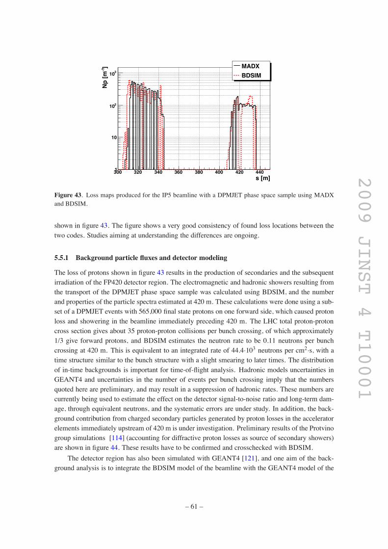
2009 JINST 4 T10001
s [m]300 320 340 360 380 400 420 440
]-1
Np
[m
1
10
210
310MADXBDSIM
Figure 43. Loss maps produced for the IP5 beamline with a DPMJET phase space sample using MADXand BDSIM.
shown in figure 43. The figure shows a very good consistency of found loss locations between thetwo codes. Studies aiming at understanding the differences are ongoing.
5.5.1 Background particle fluxes and detector modeling
The loss of protons shown in figure 43 results in the production of secondaries and the subsequentirradiation of the FP420 detector region. The electromagnetic and hadronic showers resulting fromthe transport of the DPMJET phase space sample was calculated using BDSIM, and the numberand properties of the particle spectra estimated at 420 m. These calculations were done using a sub-set of a DPMJET events with 565,000 final state protons on one forward side, which caused protonloss and showering in the beamline immediately preceding 420 m. The LHC total proton-protoncross section gives about 35 proton-proton collisions per bunch crossing, of which approximately1/3 give forward protons, and BDSIM estimates the neutron rate to be 0.11 neutrons per bunchcrossing at 420 m. This is equivalent to an integrated rate of 44.4·103 neutrons per cm2·s, with atime structure similar to the bunch structure with a slight smearing to later times. The distributionof in-time backgrounds is important for time-of-flight analysis. Hadronic models uncertainties inGEANT4 and uncertainties in the number of events per bunch crossing imply that the numbersquoted here are preliminary, and may result in a suppression of hadronic rates. These numbers arecurrently being used to estimate the effect on the detector signal-to-noise ratio and long-term dam-age, through equivalent neutrons, and the systematic errors are under study. In addition, the back-ground contribution from charged secondary particles generated by proton losses in the acceleratorelements immediately upstream of 420 m is under investigation. Preliminary results of the Protvinogroup simulations [114] (accounting for diffractive proton losses as source of secondary showers)are shown in figure 44. These results have to be confirmed and crosschecked with BDSIM.
The detector region has also been simulated with GEANT4 [121], and one aim of the back-ground analysis is to integrate the BDSIM model of the beamline with the GEANT4 model of the
– 61 –

2009 JINST 4 T10001
x [mm]-25 -20 -15 -10 -5 0
/ m
m /
bunc
h cr
ossi
ngpN
-310
-210
-110
Protons (from p-p at the IP)Hadrons (from showers)
(from showers)-,e+e
Figure 44. Secondary particles flux at the entrance of the 420 m region downstream of IP5 (preliminaryresults). The shower source is diffractive protons, generated with DPMJET, lost on the last bending magnetbefore FP420. The surviving diffractive protons are shown too.
detector. This simulation of the complete chain will allow studies beginning with proton interac-tions at the IP, and ending with the production and reconstruction of tracks in the detector stations.
The GEANT 4 geometry of the detector pockets is shown in figure 45. In the GEANT4simulations to-date, different layout of the detector stations and surrounding pockets have beenconsidered, along with different numbers of sensitive planes. In all cases the rate of secondaryinteractions of 7 TeV protons traversing the full detector region was studied as a function of thematerials used and their thickness. The results of these studies are described in section 9.7, wheretheir impact on the design of the layout of the detector region is discussed.
5.6 Machine background summary
The machine-induced background contribution at 420 m from near beam-gas and the betatroncleaning collimation is expected to be small, due to the arguments given in this section. How-ever, there is a contribution to the background rate arising from far beam-gas, the momentumcleaning collimators and proton loss in the beamline. The first two of these contributions give aproton background which is described by a peak determined by the momentum cleaning collimatorsettings, and a tail dominated by far beam-gas halo protons. The combined distribution is shown infigure 40. At detectors transverse distance of 5 mm or greater, the expected integrated number ofprotons from beam halo is expected to be less than 1 per bunch crossing. The impact of a rate ofless than 1 proton per bunch crossing on the FP420 physics signal in a pixel detector requires fur-ther study and comparison of the background and signal spatial, angular and temporal distributions.This may allow some degree of background rejection.
The proton loss background contribution is a mixture of charged and neutral particles producedimmediately upstream of 420m. The BDSIM estimate of the neutron rate is 0.11 neutrons per bunchcrossing at 420 m. The impact of these preliminary neutral background rates will be assessed interm of detector performance and survivability.
– 62 –

2009 JINST 4 T10001
Figure 45. An example of the GEANT 4 geometry of the pocket hosting the detectors. This model was usedto study the interaction rate of 7 TeV protons, which is described in section 9.7.
In summary, the preliminary proton and neutron background rates at 420 m have been esti-mated and need to be combined with detailed detector and signal studies to understand the impacton the FP420 experiment.
6 A new connection cryostat at 420 m
The LHC beamline layout downstream of an interaction point (IP) consists of a triplet of low-beta quadrupole magnets, two beam separation dipoles and a matching section of quadrupoles upto quadrupole Q7. This is followed by a dispersion suppressor region of standard dipoles andquadrupoles and finally the periodic lattice of the arc. In the dispersion suppressors there is a 14m drift space, sometimes called the “missing magnet” drift space, which is approximately 420 mdownstream of the IP. In the LHC it was decided, mainly for cost reasons, to place the dispersionsuppressors and arc magnets in one continuous cryostat from Q7, all the way to the symmetricQ7 quadrupole upstream of the next IP [124]. At the position of the missing magnet, 420 mdownstream of each IP, there is a 14 m long Connection Cryostat (CC) which contains cold beam-pipes, the 2K heat exchanger, or X-line, and various cryo-lines which run throughout the continuouscryostat, as well as the superconducting busbars and nearly 100 superconducting cables of themain bending magnets and corrector magnets. There are sixteen CCs in the LHC, each madeto be as similar as possible to a standard arc cryostat, as far as interconnection and handling areconcerned. At this 420 m point, the dispersion function D, with the standard high luminosity optics,is approximately 2 m and hence protons from the IP which have lost around 1% of their momentumare well separated from the circulating beam, as described in section 4. Placing detectors directlyinside the 1 m diameter cryostat at a temperature of 2K was considered, but ultimately dismissed,
– 63 –

2009 JINST 4 T10001
Figure 46. The new connection cryostat for FP420
primarily because of the inevitable very high local heat load on the LHC cryogenic system. Thealternative is to replace the existing connection cryostat with a warm beam-pipe section and acryogenic bypass. At the end of each arc cryostat of the LHC there is a special short cryostat calledan Arc Termination Module (ATM) which includes cold to warm transitions for the beampipes andconnects cryo-lines and superconducting busbars and cables to the electrical feed boxes. A NewConnection Cryostat (NCC) with approximately 8 m of room temperature beam-pipes has beendesigned using a modified ATM at each end.
In addition to the two modified ATMs and warm beam-pipes, the NCC shown in figure 46 hasa small cross section cryostat below the beam-pipes carrying all the cryo-lines and superconductingcircuits and a new specially designed cryostat for the X-line. All this is supported by two longi-tudinal beams to make a single unit which can be directly exchanged for an existing connectioncryostat. The passage of the X-line through the ATM modules is the main modification neededto the standard ATMs, but the geometrical layout of this passage has been arranged to be as faraway as possible from the downstream beam-pipe and hence leave adequate space for near-beamdetectors and their associated equipment. The cross-section of the NCC, with the space around thebeam-pipes available for detectors and associated mechanics, is shown in figure 47.
The existing connection cryostat contains a box structure of lead plates of 15 mm thicknessenclosing the two beam-pipes to reduce the radiation field in the tunnel, essentially replacing theshielding provided by the cold mass in a standard arc dipole cryostat. The same thickness oflead shielding will be provided around the warm beam-pipes and detector stations of the NCC. Apreliminary design, which provides a complete radiation shield while giving access to the detectorstations and passages for services is shown in figure 48.
– 64 –

2009 JINST 4 T10001
Figure 47. Cross-section view of the new connection cryostat for FP420
There are also short lengths of cylindrical shielding in the form of collars around the beam-pipes at each end of the existing connection cryostat to limit the risk of quenching adjacent super-conducting magnets. These same collars will be incorporated into the modified ATM’s at each endof the NCC in order to ensure that the performance of the NCC is also equal to the existing cryostatin terms of influence on the local radiation fields.
The engineering design of the new connection cryostat is in progress in the CERN centraldesign office of the TS/MME group. The design aim is to meet or exceed the same specificationsas the existing connection cryostat, whilst providing the maximum useable space for the FP420detectors. The preliminary design offers acceptable solutions for all cryogenic and mechanical en-gineering aspects as well as integration into the LHC environment [125, 126]. The final cryogenicperformance will depend on the detailed design, but it has already been established that the addi-tional static heat load arising from the two additional cold to warm transitions will be tolerable forthe LHC cryogenic system. In fact, simulations show that during LHC operation the NCC actuallyhas a lower dynamic heat load than the existing connection cryostat, because in the 8 m long warmsection synchrotron radiation will be absorbed at room temperature.
The detailed design of this second generation connection cryostat is in progress and will be fol-lowed by an Engineering Change Request (ECR) submitted to allow a detailed engineering reviewof all machine aspects to be performed. Following acceptance of the ECR it would in principle bepossible to build two complete NCC’s in about a year and have them tested and ready for instal-lation in late 2009. Vittorio Parma of the AT Department’s MCS group has accepted to take upresponsibility for the cryostat. He will lead a working group which will verify the compatibility ofthe existing conceptual design and develop the detailed design for manufacture. As regards con-struction of the NCC’s, the sixteen ATM modules of the LHC were assembled at CERN in a ded-icated workshop in Building 110, under the responsibility of Ramon Folch (TS/MME). His teamhas prepared a preliminary construction schedule and cost estimate for the new cryostats [127].
– 65 –

2009 JINST 4 T10001
Figure 48. Preliminary design for radiation shielding around the warm beampipes and detector stations. Themobile shielding can be rolled sideways on rails to give access to the detector stations.
The cutting and removal of the existing connection cryostat and its replacement by an NCCis very similar to the replacement of a standard LHC dipole and has been evaluated by the groupresponsible for all the LHC interconnections. As mentioned above this is the same group that tookresponsibility for the design installation and performance of the existing connection cryostat.
Table 11 shows the sequence of operations and the estimated time needed in normal workingdays to complete the exchange of a connection cryostat from start of warm-up to being ready forbeam. It is thus conceivable that the installation of FP420 modules consisting of an NCC cryostatand associated detectors could be completed in an annual long shutdown. A preliminary studyof the transport aspects has shown that adequate tooling exists and it can be expected that thetime needed will be in the shadow of other operations shown in table 11. However, the number ofconnection cryostats that can be replaced in a standard annual shutdown will depend on the numberof LHC magnets requiring replacement and the work load of the interconnection teams.
6.1 Cryostat summary
In summary, a preliminary design for a replacement connection cryostat that would allow detectorsto be placed in the 420 m region has been completed, and a final design is in progress. This solutionis expected to actually lower the dynamic heat load of the LHC and have similar radiation profiles.With the appropriate approvals and funding, two such cryostats could be built and installed in late2009, and in principle, two more in 2010 with negligible risk to LHC operations.
– 66 –

2009 JINST 4 T10001
Table 11. The estimated time in days required to install one NCC.
Normal DaysWarmup from 1.9K to 4.5 K 1Warmup from 4.5K to 300 K 15
Venting 2Dismantling interconnection 10
Removal of the connection cryostat 2Installation of the FP420 cryostat 5Realization of the interconnections 15
Leak test and electrical test 4Closing of the vacuum vessel 1
Evacuation/repump 10Leak test 2Pressure test 4
Cool-down from 300 K to 4.5 K 15Cool-down from 4.5K to 1.9 K 3
Total [days] 89
7 Hamburg beam-pipe
7.1 Introduction
Detection of diffractive protons at 420 m from the IP is particularly challenging since it requiresdetectors to be placed between the two LHC beam-pipes, the exteriors of which are separated byabout 140 mm (the distance between the pipe axes is nominally 194 mm). In addition, the nearbycryogenic lines severely limit the available free space. Due to these space constraints the traditionalRoman Pot (RP) technique cannot be used, and another concept for near beam detectors, pioneeredat DESY is proposed. This technique of moving sections of beam-pipe with integrated detectors isknown as “Hamburg pipes” and was developed within the ZEUS collaboration in 1994 to measurevery forward-scattered electrons as a signature of photoproduction [128]. The concept was inspiredby the moving pipes used in the PETRA wiggler line to allow for beam-line aperture changes. TheZEUS version involved small electromagnetic calorimeters attached to the moving pipe (44 m fromthe interaction point). The detectors were retracted during beam injection, but could be positionedclose to the beam axis during stable beam conditions, and thus measure scattered electrons with re-duced energy, which exited the pipe through special thin windows. Since the detectors were locatedoutside of the machine vacuum, they could be easily maintained and were successfully and rou-tinely used for six years, providing data essential for several publications [129]. The detectors werepositioned remotely by the HERA shift crew, which inserted the detectors at the working position,typically about 15 mm from the coasting electron beam, using the HERA slow control system.
– 67 –

2009 JINST 4 T10001
Figure 49. Schematic view of the connection cryostat (1) and detector arm with support table (2), twodetector sections (3) and vacuum pumping sections (4).
Prior to installation at HERA, the Hamburg pipe system was tested by making several thousanddisplacement operations. No significant radio-frequency (RF) effects on the electron beam wereobserved due to the modified beam-pipe geometry. It should be noted that no special RF screeningwas used; it was sufficient to have the so-called RF fingers providing good electrical contact acrossthe connecting bellows.
The moving pipe technique has many advantages with respect to the RP design. It allows muchsimpler access to detectors and provides direct mechanical and optical control of the actual detectorpositions. In addition, unlike the Roman pot case which involves forces from pressure differencesas the detectors are inserted into the vacuum, the Hamburg pipe maintains a fixed vacuum volume.This results in much less mechanical stress, consequently allowing a very simple and robust design.
7.2 FP420 moving pipe design
A modified connection cryostat (section 6) has been designed with approximately eight meter longwarm beam-pipes, providing adequate lateral space to install the FP420 detectors. Figure 49 showsthe layout of the connection cryostat including two detector stations and the support table. Theentire detector arm is fixed on the support table, which is attached to the tunnel floor, independent ofthe cryostat. Both ends of the detector arm are equipped with vacuum pumping and control stationsand isolation valves. Figure 50 shows one of the two detector stations equipped with timing andsilicon detectors, an LVDT (Linear Variable Differential Transformer) for position measurementand one moving and one fixed beam position monitor (BPM). The support table and motion systemare shown in figure 51.
The basic dimensions of the stations are defined by the LHC standard beam-pipe diameter, therequired lateral detector translation, and by the longitudinal dimensions of the FP420 detectors.
– 68 –

2009 JINST 4 T10001
Figure 50. Top view of one detector section: bellows (1), moving pipe (2), Si-detector pocket (3), timingdetector (4), moving BPM (5), fixed BPM (6), LVDT position measurement system (7), emergency springsystem (8).
Each station is composed of a beam-pipe with inner diameter of 68.9 mm, wall thickness of3.6 mm and a length of about 1000 mm, fixed on a motorised drive. Rectangular thin-walledpockets are built into the pipe to house the different detectors that must be positioned close tothe beam. The displacement between data taking position and the retracted or parked position isabout 25 mm. The ends of the moving beam-pipes are connected to the fixed beam-pipes by aset of two bellows. Inside, these may be equipped with moving RF-contacts to assure electricalcontinuity. In general, this design allows significant flexibility in the configuration of the detectorsstations, allowing optimization of the detector operation, scattered proton detection, kinematicalreconstruction, and alignment.
7.3 Pocket design and tests
A key factor in the pocket design is the desire to maximise detector acceptance, which is achievedby minimizing the distance of the detector edge from the LHC beam. This in turn requires thatthe thickness of the detector pocket wall should be minimised to limit the dead area. Care must betaken to avoid significant window deformation which could also limit the detector-beam distance.
A rectangular shaped detector pocket is the simplest to construct, and minimises the thin win-dow material perpendicular to the beam which can cause multiple scattering and degrade angularresolution of the proton track. RF studies of the rectangular pocket have shown (see section 8) thatthe effects on the beam dynamics are minor. For reasons of mechanical stiffness, thermal stabilityand fabrication of the pockets, only stainless steel beam tubes are suitable. They will be coppercoated for RF-shielding and Non-Evaporative Getter (NEG) coated for vacuum pumping. A rect-angular slot of adequate height and length is machined in the beam tube. A thin window is then
– 69 –

2009 JINST 4 T10001
Figure 51. Support table (1), drive support table with alignment system (2), drive motor (3), intermediatetable for emergency withdrawal (4), moving support table (5), and linear guides (6).
Figure 52. Interior of the moving beam-pipe as seen by the particles.
welded in this slot. Both welded and extruded pipes have been used in tests. Figure 52 shows theinterior of the Hamburg pipe including the thin vacuum window as seen by the scattered protons.
First tests using welded pipes showed excessive deformation due to asymmetrical stressesappearing after the machining of the cylindrical pipes. Several welding techniques for differentlength pockets have been considered and two have been tested: Tungsten Inert Gas (TIG) weldingand laser welding, the latter expected to produce somewhat smaller deformation. A first prototypeused thin (0.2 and 0.3 mm)windows of 83 mmheight and 200 mm length TIGwelded in rectangularslots, machined in a tube of diameter 89 mm. The deformation for this setup under vacuum wereunacceptable, exceeding 5 mm in the centre. Pressure tests with this prototype have shown that theTIG weld is quite strong, as it supported pressures of up to 7 bar.
– 70 –
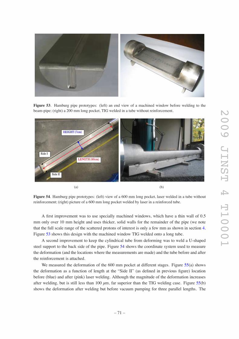
2009 JINST 4 T10001
Figure 53. Hamburg pipe prototypes: (left) an end view of a machined window before welding to thebeam-pipe; (right) a 200 mm long pocket, TIG welded in a tube without reinforcement.
(a) (b)
Figure 54. Hamburg pipe prototypes: (left) view of a 600 mm long pocket, laser welded in a tube withoutreinforcement; (right) picture of a 600 mm long pocket welded by laser in a reinforced tube.
A first improvement was to use specially machined windows, which have a thin wall of 0.5mm only over 10 mm height and uses thicker, solid walls for the remainder of the pipe (we notethat the full scale range of the scattered protons of interest is only a few mm as shown in section 4.Figure 53 shows this design with the machined window TIG welded onto a long tube.
A second improvement to keep the cylindrical tube from deforming was to weld a U-shapedsteel support to the back side of the pipe. Figure 54 shows the coordinate system used to measurethe deformation (and the locations where the measurements are made) and the tube before and afterthe reinforcement is attached.
We measured the deformation of the 600 mm pocket at different stages. Figure 55(a) showsthe deformation as a function of length at the “Side II” (as defined in previous figure) locationbefore (blue) and after (pink) laser welding. Although the magnitude of the deformation increasesafter welding, but is still less than 100 µm, far superior than the TIG welding case. Figure 55(b)shows the deformation after welding but before vacuum pumping for three parallel lengths. The
– 71 –

2009 JINST 4 T10001
(a)
(b)
Figure 55. (a) Deformation as a function of length at the “Side 2” location before (blue) and after (pink)laser welding. (b) Deformation after welding but before vacuum pumping for the three locations.
effect is similar, although it is a little worse in the middle (blue) than in the two sides, as expected,it is still less than 100 µm. Figure 56(a) shows that although the deformation at the sides (edges) isnot much affected by vacuum pumping, it becomes much larger (> 300 µm) in the middle. Afterreinforcement, however, it is reduced to acceptable levels, as shown by the perpendicular heightprofile at the middle of the tube in Figure 56(b). We also note that the final design will have pocketsof 1/3 to 1/2 the length, implying significantly less deformation.
– 72 –

2009 JINST 4 T10001
(a)
(b)
Figure 56. (a) Deformation as a function of length after vacuum pumping. (b) Height profiles after rein-forcement.
A new 1 micron-precision 3D multisensor measuring device has been tested on a 200 mm longTIG welded window. The result is shown in figure 57. This device will help us fully evaluate thefinal prototypes.
Two prototype beam tubes equipped with 600 mm long pockets were used for RF measure-ments at the Cockcroft Lab. The results of these measurements are described in section 8.
– 73 –

2009 JINST 4 T10001
0
10
20
30
40
50
60
70
80
90
10
0
11
0
12
0
13
0
14
0
15
0
16
0
Y=0
Y=3
Y=6
Y=9
Y=12
74,7
74,8
74,9
75
75,1
75,2
75,3
75,4
75,5
Heigh of surface
Length of pocket
Height of pocket
Evolution of the Surface
Y=0
Y=1
Y=2
Y=3
Y=4
Y=5
Y=6
Y=7
Y=8
Y=9
Y=10
Y=11
Y=12
Y=13
Y=14
Figure 57. Example of a 3D profile measurement run using the multi sensor equipment.
7.4 Test beam prototype
The baseline prototype of the moving beampipe was prepared for use in test beam at CERN inOctober 2007. Figure 58 shows the 1 m long beam-pipe equipped with two pockets, one of 200mm length for the 3D pixel detector (section 9) and the other of 360 mm length for the gas Cerenkovtiming detector (section 10) . The vacuum window thickness was 0.4 mm. A detector box for the3D detectors was mounted in the first pocket. The moving pipe was fixed on a moving table, drivenby a MAXON motor drive and guided by two high precision linear guides. The moving table wasequipped with alignment adjustments in the horizontal, vertical, and axial (along the beam axis)directions, and was attached to a fixed structure in the test beam area. The relative position of themoving pipe was measured with two SOLARTRON LVDT displacement transducers, which have0.3 µm resolution and 0.2% linearity.
7.5 Motorization and detector system positioning
In routine operation, detector stations will have two primary positions (1) the parked position duringbeam injection, acceleration and tuning, and (2) close to the beam for data taking. The positioningmust be accurate and reproducible. Two options have been considered: equipping both ends ofthe detector section with a motor drive which are in principle moving synchronously but allowingfor axial corrections with respect to the beam axis, or a single drive at the centre, complementedwith a local manual axial alignment system. A two motor solution in principle allows perfectpositioning of the detector station, both laterally and axially. However, it adds complexity to the
– 74 –

2009 JINST 4 T10001
Figure 58. Photograph of the prototype beam-pipe section used in the October 2007 CERN test beam.
control system, reduces reliability, and increases cost. Positioning accuracy and reproducibility arealso reduced because extremely high precision guiding systems can no longer be used, due to thenecessary additional angular degree of freedom. Therefore, a single motor drive system has beenchosen, accompanied by two precise LVDTs. As in the LHC collimator system, no electronicsis foreseen in highly irradiated zones, close to the motors, to limit radiation damage. For ease inintegration, we are planning to adopt the collimator stepping motor solution. As these have neverbeen irradiated, the stepping motors will be tested in the high neutron flux test beamline at theLouvain-la-Neuve cyclotron centre CRC [130].
7.6 System operation and safeguards
Given the FP420 schedule, it will be possible to learn from the experience that will be gainedduring the LHC commissioning by the operation of machine elements with similar control andsurveillance aspects, namely the TOTEM [131] and ATLAS ALFA Roman Pot [132] detectorsand the LHC collimators [133]. Nevertheless a series of aspects specific to FP420 need to beaddressed. The F420 detectors will operate at all times in the shadow of the LHC collimators inorder to guarantee low background rates and to avoid detector damage from unwanted beam losses.In addition, for machine protection constraints, it will be unacceptable for FP420 to interfere withthe beam cleaning system (e.g. to avoid magnet quenches downstream the 420 m region).
Therefore, the high-level Hamburg pipe control system will be integrated in the collimatorcontrols. The interface between low- and high-level controls will be implemented with the CERNstandard Front End Standard Architecture (FESA) [134].
– 75 –
2009 JINST 4 T10001
The Main Control Room will position the detectors close to the beam after stable collisionsare established. The precision movement system will be able to operate at moderate and very lowspeed for positioning the detectors near the beam. During insertion and while the detectors are inplace, rates in the timing detectors will be monitored, as well as current in the silicon. The stepmotor and LVDT’s will provide redundant readback of the position of the detectors and the fixedand moveable BPM’s will provide information on the position of the detectors with respect to thebeam. Separate mechanical alignment of the height and orientation with respect to the beam arediscussed in section 11.
7.7 Hamburg pipe summary and outlook
The Hamburg moving pipe concept provides the optimal solution for the FP420 detector systemat the LHC. It ensures a simple and robust design and good access to the detectors. Moreover, itis compatible with the very limited space available in the modified connection cryostat and withthe expected position of the scattered protons between the two LHC beampipes. Its reliability islinked to the inherent absence of compensation forces and the direct control of the actual positionof the moving detectors. Finally, rather large detectors, such as the timing devices, can naturally beincorporated using pockets, rectangular indentations in the moving pipes. The prototype detectorpockets show the desired flatness of the thin windows, and the first motorised moving section,with prototype detectors inserted, has been tested at the CERN test beam. This was a first stepin the design of the full system, including assembling, positioning and alignment aspects. A fullprototype test is planned in test beam in Fall 2008.
We want to stress that the moving pipe design development and prototyping has been donein direct contact with the LHC cryostat group. In particular, the Technical Integration Meetings(TIM), held regularly at CERN and chaired by K. Potter, provided an efficient and crucial frame-work for discussions and information exchanges.
8 RF impact of Hamburg pipe on LHC
8.1 Motivation and introduction
The electromagnetic interaction between the beam and its surroundings will be one of the phe-nomena limiting the ultimate performance of the LHC, because it can lead to single bunch andmulti-bunch beam instabilities, beam emittance growth and beam losses. Usually such effects areexpressed in terms of wake fields and beam coupling impedance. As discussed in the LHC designreport [124], the LHC has an overall impedance budget that requires careful design of each elementof the accelerator to minimise the total impedance. During the first years of operation, it is expectedthat the maximum intensity of the LHC colliding beams will be limited by collimation efficiencyand impedance effects; consequently a series of studies designing upgraded configurations of theLHC was initiated many years ago. The primary focus of these studies is the collimation system,since it is the dominant component of the impedance budget.
In general, the electromagnetic effects are enhanced by the use of low electric conductiv-ity materials, by small distances between the beam and the vacuum chamber and by any trans-verse cross section variation of the vacuum chamber. In particular, the transverse resistive wall
– 76 –

2009 JINST 4 T10001
Figure 59. The two benchmark FP420 pocket designs. The upper figure is a single pocket solution. Thelower figure is a double pocket design, which will allow separate temperature and vacuum conditions fortiming and silicon detectors
impedance [135, 136] increases when the beam approaches the beam pipe wall, which will reg-ularly occur during FP420 detector insertion. Both the real and imaginary part of the transverseimpedance have to be controlled, in order to minimise the effect on beam instability growth rateand betatron tune shift.
Variation of the beam pipe cross-section in the 420 m region not only is a potential issue forLHC operations through increased impedance, but it can also affect the FP420 detectors. Trappedmodes arising from the exchange of electromagnetic energy between the beam and its surround-ings can cause heating of the detectors which increase their cooling requirements, since they mustoperate at low temperature. Moreover, the electromagnetic fields can penetrate through the beampipe walls and be picked up by the detector electronics.
We have begun a series of studies to examine the different aspects of the FP420 impedance.Analytical calculations and numerical simulations are underway to assess the longitudinal andtransverse impedance values. Laboratory measurements on an FP420 station prototype have beenperformed to validate the simulations and will serve to investigate the effect of electromagneticdisturbances on the detector electronics. These studies are also useful to suggest modifications tothe final FP420 design to minimise RF effects.
During LHC operation, the real effect of wake fields on power losses and beam instabilitywill be assessed by the convolution in the frequency domain between the beam spectrum and thecoupling impedance. Therefore, the relevant upper limit on the frequency that must be consideredis assessed by the nominal LHC beam bunch length, σz = 0.25 ns (r.m.s.). This permits us to limitour study up to a frequency of 3GHz. The following sections describe the current status of theRF studies.
8.2 Longitudinal impedance
Most of the studies are based on the stretched wire method for evaluating the longitudinal couplingimpedance ZL through the measurement of the scattering parameters of the network composed byan RF source and the device under test (DUT) [137]. Usually, the RF source is a two ports VectorNetwork Analyzer that is used to send an electromagnetic wave through the wire stretched along
– 77 –

2009 JINST 4 T10001
the DUT. The measurement consists in determining the scattering parameter S21, that is defined asthe ratio of the output of the VNA port 2 to the incident wave on port 1. With such a method, thedeviation of the impedance of the DUT from that of a reference vessel (REF) can be modeled with aloaded transmission line [138]. Solving the resulting non-linear equation to first order in impedanceenables an explicit relation (as function of frequency f ) between the longitudinal impedance ZL andS21 to be obtained. This is referred to as the “log” formula:
"ZL( f ) = $2Zc ln"SDUT21 ( f )"SREF21 ( f )
, (8.1)
where Zc is the characteristic line impedance.The results will be expressed in terms of longitudinal impedance ZL/n:
"
ZLn
#
=ZL( f )f/ f0
, (8.2)
where n = f/ f0 and f0=11 kHz is the beam revolution frequency in the LHC. This quantity can becompared to predictions and measurements of other LHC elements, as reported in [124]. All thecalculations and measurements refer to an FP420 pocket made of stainless steel.
8.2.1 Simulations
Figure 59 shows two beam pipe designs considered for the RF simulations, a single long pocketand an alternative design with two shorter pockets. The results of three different numerical sim-ulation packages are presented. Ansoft HFSS c! [139] was used to simulate the stretched wiresetup and calculate the longitudinal impedance according to eq. (8.1), while CST Particle Studio c!
(PST)13 [140] and GDFIDL [141] provide a direct calculation of the electromagnetic field inducedby a passing bunch on the surrounding structure.
Figure 60 shows, for all three simulations, the calculations of the real and imaginary parts ofthe longitudinal impedance. For the single pocket geometry, four narrow band impedance peaks areobserved between 2.4 and 2.75 GHz for the HFSS and PST simulations. The frequency differenceis attributed to the presence of the wire in the HFSS simulation. Two of the four resonances aresignificantly reduced for the double pocket simulation with GDFIDL. The wide band resonancesthat we observe (in both HFSS simulations and experiment) for f < 2.4GHz are understood tobe an artifact of the wire and do not represent a real beam impedance effect. Simulations of thedouble pocket geometry with HFSS are in progress and preliminary results confirm the laboratoryexperiments that are presented in the next section.
8.2.2 Laboratory measurements
The laboratory setup at the Cockcroft Institute comprises a sophisticated mechanical systemequipped with micrometer screws, in order to stretch, move and monitor the relative position ofthe wire. A set of measurements in the time domain was used to determine the absolute position ofthe wire with respect to the pocket wall with an accuracy of about 100µm [142].
13In performing these simulations, a beta-version of PST has been used.
– 78 –

2009 JINST 4 T10001
f [GHz]2 2.1 2.2 2.3 2.4 2.5 2.6 2.7 2.8 2.9 3
]Ω
)/n [m
LR
e(Z
-310
-210
-110
1
10
210ANSOFT HFSS
CST Particle Studio (no wire)
GDFIDL (no wire, double-pocket, courtesy of W.Bruns)
f [GHz]2 2.1 2.2 2.3 2.4 2.5 2.6 2.7 2.8 2.9 3
]Ω
)/n [m
LIm
(Z
-10
-5
0
5
10
15ANSOFT HFSS
CST Particle Studio (no wire)
GDFIDL (no wire, double-pocket, courtesy of W.Bruns)
Figure 60. Real (left) and imaginary part (right) of the longitudinal impedance for three different simulationsof the single pocket prototype, effectively assuming the pocket wall is 3 mm away from the beam.
f [GHz]2.2 2.3 2.4 2.5 2.6 2.7 2.8 2.9 3
]Ω
)/n [m
LR
e(Z
-310
-210
-110
1
10
210MeasurementsMeasurements, Cu Tapering
HFSS simulations
f [GHz]2.2 2.3 2.4 2.5 2.6 2.7 2.8 2.9 3
]Ω
)/n [m
LIm
(Z
-4
-2
0
2
4
6
8
10MeasurementsMeasurements, Cu Tapering
HFSS simulations
Figure 61. Measurements of real (left) and imaginary part (right) of the longitudinal impedance with thebeam 3mm from the pocket wall for the single pocket prototype; also shown are the HFSS simulations.
Single pocket results. The real and imaginary part of the FP420 longitudinal impedance calcu-lated from the measured S21 parameter (black solid line) and simulated by HFSS (blue dashed line)are shown in figure 61. This plot refers to a wire distance from the pocket wall of 3mm, simu-lating a detector 3 mm (10σx) from the beam. Measurements and simulations have been carriedout for several intermediate distances from this position of closest approach to a retracted position(x > 50σx from the beam).
The agreement between measurements and simulations, in terms of resonance peaks of theimpedance is satisfactory as they lie within 3mΩ in amplitude and a few MHz in frequency. Atleast one additional resonance appears in the measurements (e.g. at 2.75GHz) and can be explainedby a residual mismatch between the RF source and the DUT, not considered in the simulations.
The FP420 pocket was remeasured after applying a thin copper-plated tape at the indentationregions. The tape was placed outside the beam orbit region (i.e. above and below the 500 µm thinwindow), in order to provide a tapered transition of the beam pipe cross section variation. Theresult is shown by the red solid lines in figure 61. After tapering, the longitudinal impedance isreduced by an order of magnitude and thus the impedance is limited to no more than 1mΩ over the
– 79 –

2009 JINST 4 T10001
f [GHz]2.3 2.35 2.4 2.45 2.5 2.55 2.6 2.65 2.7
]Ω
/n) [
mL
Re(
Z
-110
1
10
Before tapering
After tapering
Double pocket, retracted position
f [GHz]2.3 2.35 2.4 2.45 2.5 2.55 2.6 2.65 2.7
]Ω
/n) [
mL
Re(
Z
-110
1
10
Before tapering
After tapering
Double pocket, physics position (wire at 3mm)
f [GHz]2.3 2.35 2.4 2.45 2.5 2.55 2.6 2.65 2.7
]Ω
/n) [
mL
Im(Z
-10
-8
-6
-4
-2
0
2
4
6
8
10Before tapering
After tapering
Double pocket, retracted position
f [GHz]2.3 2.35 2.4 2.45 2.5 2.55 2.6 2.65 2.7
]Ω
/n) [
mL
Im(Z
-10
-8
-6
-4
-2
0
2
4
6
8
10Before tapering
After tapering
Double pocket, physics position (wire at 3mm)
Figure 62. Real and imaginary part of the longitudinal impedance for the FP420 physics (inserted) andparking positions, as measured for a double pocket prototype.
measured frequency band.
Double pocket results. A first set of laboratory measurements with an FP420 double pocket pro-totype has been completed. The results are shown in figure 62 in terms of the real and imaginarypart of the longitudinal impedance and for parking and physics positions. The black dashed linesrefer to the original beam pipe, whereas the solid red lines assess the measured impedance valueafter applying a copper tape at the accessible pockets indentations (i.e. for each pocket, the in-dentation at the beam pipe end). The two indentations in between the two pockets are not easilyaccessible after the beam pipe fabrication and could not be tapered or connected with an RF contactduring these measurements. As for the single pocket prototype, there are no impedance peaks forfrequencies below 2GHz. After tapering, the real part of the longitudinal ZL/n impedance remainsabove 5mΩ at about 2.46GHz, when the detectors are 3mm from the beam. In all the rest of thefrequency band of interest, both the real and imaginary parts of the longitudinal impedance arebelow 5mΩ.
8.3 Transverse impedance and beam instability
The transverse impedance can be inferred by the variation of the longitudinal impedance for dif-ferent wire (beam) transverse positions. Figure 63 compares the simulated transverse impedancewith an analytical prediction accounting for resistive wall effects only. The results are in goodagreement since the oscillation at low frequencies given by the numerical simulations is attributed
– 80 –
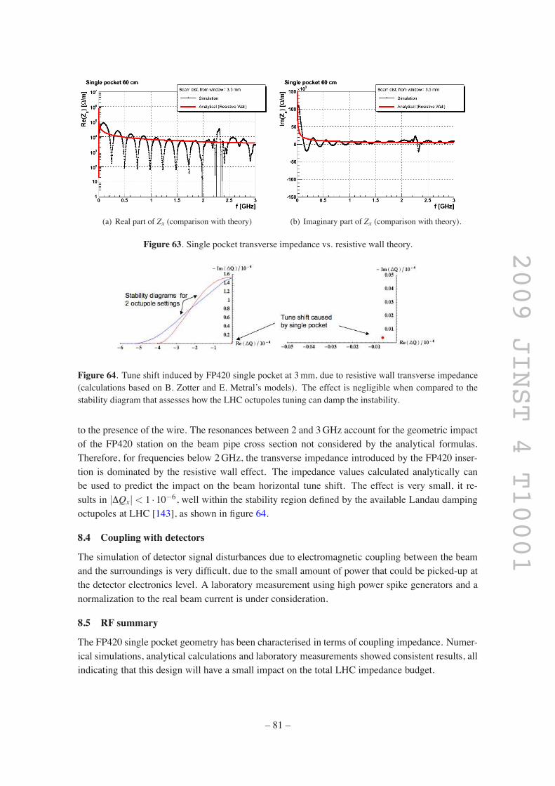
2009 JINST 4 T10001
(a) Real part of Zx (comparison with theory) (b) Imaginary part of Zx (comparison with theory).
Figure 63. Single pocket transverse impedance vs. resistive wall theory.
Figure 64. Tune shift induced by FP420 single pocket at 3mm, due to resistive wall transverse impedance(calculations based on B. Zotter and E. Metral’s models). The effect is negligible when compared to thestability diagram that assesses how the LHC octupoles tuning can damp the instability.
to the presence of the wire. The resonances between 2 and 3GHz account for the geometric impactof the FP420 station on the beam pipe cross section not considered by the analytical formulas.Therefore, for frequencies below 2GHz, the transverse impedance introduced by the FP420 inser-tion is dominated by the resistive wall effect. The impedance values calculated analytically canbe used to predict the impact on the beam horizontal tune shift. The effect is very small, it re-sults in |ΔQx| < 1 ·10$6, well within the stability region defined by the available Landau dampingoctupoles at LHC [143], as shown in figure 64.
8.4 Coupling with detectors
The simulation of detector signal disturbances due to electromagnetic coupling between the beamand the surroundings is very difficult, due to the small amount of power that could be picked-up atthe detector electronics level. A laboratory measurement using high power spike generators and anormalization to the real beam current is under consideration.
8.5 RF summary
The FP420 single pocket geometry has been characterised in terms of coupling impedance. Numer-ical simulations, analytical calculations and laboratory measurements showed consistent results, allindicating that this design will have a small impact on the total LHC impedance budget.
– 81 –

2009 JINST 4 T10001
Tapering of the beam pipe indentations is recommended because it does reduce the impedancesignificantly, as measured both with the single pocket and double pocket designs. Since an effectivetapering can be done outside the beam orbit region, this design modification can be implementedat no cost in terms of the forward proton signal to background ratio. With a double pocket stationdesign, the beam pipe section between the two pockets can also be electrically connected outsidethe beam orbit region, in order to provide a good RF contact and minimise the effect of beampipe cross section variation. This could not be tested in the laboratory, due to the difficulty ofaccessing the region after beam pipe fabrication. Simulations and laboratory measurements of anew prototype, modified according to the RF studies completed so far, will be continued.
The resultant effective longitudinal impedance follows from the convolution of the resultspresented here with the LHC beam spectrum. The beam harmonics at 2GHz are expected to bebelow 10$2 of the main harmonic at 40MHz and well below 10$3 at 2.5 GHz. This provides afurther indication of the expected minimal impact of a FP420 station on the LHC impedance. Oneof the consequences is that, according to the available analytical models, the horizontal tune shiftinduced by a FP420 station is expected to be almost imperceptible when compared to the tunestability region defined by the available LHC octupoles magnets.
In addition, the worst case considered in these studies, refers to the positioning of a FP420station at 3mm from the circulating beam, whereas recent acceptance (section 4) and background(section 5) calculations indicate that 5mm is a more likely distance of closest approach. Thisimplies that the results are conservative in terms of disturbances to the beam. Further studies areongoing in order to determine the characteristic loss factor, which will provide an estimate of thepower dissipated due to electromagnetic coupling.
9 Silicon Tracking Detectors
9.1 Introduction
In order to detect protons from the production of central systems of masses # 100 GeV/c2, thedetector edge has to approach the beam axis to a distance of 5 mm (see figure 28). This representsa challenge for the radiation hardness and radio-frequency pick-up in the detector and the nearbyfront-end electronics, as described in sections 5 and 8. The detector system has to be robust, andfor satisfactory control of systematic uncertainties its position has to be aligned and maintained toa positional accuracy of 10 µm in order to achieve the required track angular precision of 1µrad(see section 4.3).
With a typical LHC beam size at 420 m of σbeam . 300 µm, the window surface of the Ham-burg pipe can theoretically safely approach the beam to 15 % σbeam. 4.5 mm. As discussed insection 5 however, this distance will ultimately be determined by the LHC collimator settings,since for beam 2 in particular the halo can extend to# 5 mmwith the nominal collimator positions.The window itself adds another 0.2 mm to the minimum possible distance of the detectors from thebeam. To maximise the acceptance for low momentum-loss protons, the detectors should thereforebe active as close to their physical edge as possible. In general, planar silicon detectors have a wide(0.25 mm–1 mm) insensitive border region around the sensitive area that is occupied by a sequenceof guard rings. This ring structure controls the potential distribution between the detectors sensi-tive area and the cut edge to remove leakage current. Planar silicon detectors designed for a heavy
– 82 –

2009 JINST 4 T10001
Figure 65. Isometric and lateral view sketches of a 3D detector where the p+ and n+ electrodes are processedinside the silicon bulk. The edges are trench electrodes (active edges) and surround the sides of the 3D devicemaking the active volume sensitive to within a few microns of the physical edge.
radiation environment or generally for operation at high bias voltages, contain multi-ring structureswith typically about #20 rings.
The key requirements for the FP420 tracking system are
• To track efficiently as close as possible to the sensor’s physical edge.
• To have extreme radiation hardness. A design figure equivalent to or better than the vertexsystems used for ATLAS or CMS will be required, i.e. better than 1015 1-MeV equivalentneutrons per cm2.
• To operate at the highest LHC luminosity and be robust and reliable.
• Individual detectors should have a spatial precision of #10 microns. The tracking systemangular precision should be 1 µrad. These requirements are discussed in detail in section 4.
• At 420 m the tracking detector needs to cover an area of 25 mm x 5 mm.
3D silicon technology has been chosen as the baseline detector technology best equipped tomeet the above requirements, although the tracking system has been designed such that any silicontechnology compatible with the ATLAS pixel readout can be used. The 3D silicon sensor R&D isdescribed in section 9.2. Section 9.3 discusses the mechanical design of the tracking detector, sec-tion 9.4 discusses solutions for the required high voltage and low voltage, and section 9.5 discussesthe infrastructure and readout. The thermal performance of the system is described in section 9.6.The performance of the proposed tracking system is described in section 9.7.
9.2 3D silicon detector development
3D detectors are a new generation of semiconductor devices [131, 144–156]. Using micro-machining techniques, electrodes penetrate the entire thickness of the detector perpendicular to thesurface. This results in smaller collection distances, very fast signals, and substantially improved
– 83 –

2009 JINST 4 T10001
Figure 66. Two-dimensional efficiency map of a fully operational 3D detector. A point is plotted withrespect to the position (x,y) predicted by a telescope, with a precision of 4 µm as a valid track and a hit wasrecorded by a 3D detector. The inefficient band near the lower x-edge was caused by the detector’s bondingpads. The upper and lower y edges were used for active edge measurements and showed a device sensitivityup to 4 microns from the physical edge.
radiation tolerance. Figure 65 sketches the main features of this novel detector design. In addition,similar micro-machining techniques allow one to produce “active edges” where the amount of deadsilicon at the edge of the detector is greatly reduced.
Full-3D silicon sensors have been successfully fabricated at CIS-STANFORD by J. Hasi(Manchester University) and C. Kenney (Molecular Biology Consortium) since 2001, followingthe original design of Sherwood Parker, University of Hawaii and C. Kenney who developed activeedges. The Manchester/MBC/Hawaii Collaboration has been working since 1999 to develop thistechnology for applications in particle physics. Important results are summarised below.
The first 3D detector used 16 rows of 38 p+ electrodes spaced by 100 µm. n+ electrodes wereplaced 100 mm from the p+ electrodes. The total active area was 3.2 mm by 3.9 mm. The p+electrodes were connected as strips to ATLAS SCTA readout chips. After tests in the X5 beam atthe CERN SPS in 2003, the efficiency was found to be around 98% and particles were detected towithin 5 µm of the physical edge, as can be seen in figure 66. The full results of this beam test canbe found in the TOTEM TDR [131] and ref. [156]. A hybrid technology (planar/3D) detector wasmanufactured at Stanford and was successfully tested by TOTEM in a prototype Roman Pot at theCERN SPS in 2004. This uses planar technology but has a 3D active edge. This worked well, butis a factor 100 less tolerant to irradiation than full 3D technology.
Initial tests on irradiated 3D samples were made in 2001 [148]. The first results on the signalefficiency were obtained in 2006 using signal generated by an infrared laser. The 3D deviceswere irradiated with neutrons in Prague with an equivalent fluence of 1016 protons/cm2 [155]. As
– 84 –

2009 JINST 4 T10001
Figure 67. Response of a 3 electrodes/pixel (3E) 3D device to a 1060 nm laser pulse after 3.7% 1015,5.98%1015 and 8.6%1015 neutrons/cm2.
expected, 3D devices can operate at much higher fluences than conventional silicon devices. For aminimum ionising particle, the signal size depends on the thickness. However, the signal collectiondistance is determined by the inter-electrode spacing, which can be as short as 50 microns. Themeasurement is shown in figure 67 for a 3E device with an inter-electrode distance of 71 microns.This has three n-type collection electrodes in a pixel size of 50 micron by 400 microns. Figure 68shows the signal efficiency versus fluence for the 3D detector. It is compared to the best that hasbeen achieved using strip and pixel detectors for the LHC experiments. 3D technology is about afactor five more radiation tolerant.
For the FP420 application the ATLAS Pixel Readout chip was chosen. The total active areais 7.2 mm by 8 mm. The pixel structure is shown in figure 69. The 3D detectors were bump-bonded to the readout chip. To cover the full area, a minimum of three detectors are required. Thedetails of the mechanical/electronic layout required to make a single layer with full area coverageis described in section 9.2. Figure 70 shows that the 4E device can operate at the lowest voltage.Charge sharing only occurs very close to the pixel edge. Operating voltages are a factor ten lessthan for a standard planar device. Figure 71 shows a processed 3D wafer. The device yield wasaround 80%.
2E, 3E and 4E devices, bump-bonded to ATLAS Pixel readout chip were tested in the H8beam at CERN in Autumn 2006 with support from LBL and Bonn. Individual detectors wereplaced between planes of a silicon microstrip tracking system. The beam was 100 GeV/c pions.Figure 72 shows a hit map for a 12 mm % 12 mm and 3 mm % 3 mm scintillator trigger. There
– 85 –

2009 JINST 4 T10001
Figure 68. Signal efficiency of 3D detector versus fluence of 1 MeV equivalent neutrons/cm2. Data for n onp silicon strips and n-side readout pixel detectors are shown for comparison. Diamond detector results arealso shown. Note that diamond gives a factor three less signal for a minimum ionising particle.
Figure 69. Different 3D cell structures designed to be compatible with the ATLAS Pixel detector readoutchip. The pixel size is 50 µm by 400 µm. The devices have either 2, 3 or 4 electrodes per pixel and arenamed 2E, 3E and 4E respectively. The electrodes cover 4%, 6% and 8% of the total area for 2E, 3E and 4Edevices respectively.
– 86 –

2009 JINST 4 T10001
Figure 70. Equipotentials in a 2E and 4E 3D detector. Pixel size is 50 µm (Y) by 400 µm (X). The bias is20 V and 5 V for the 2E and 4E devices respectively. The direction of the electric field is indicated. Then-electrodes are at the centre. A maximum field of 1 V/µm occurs at 24 V and 14 V in a 2E and 4E devicerespectively.
Figure 71. Four-inch wafer processed for the FP420 project. This has 32 3E, 6 4E and 6 2E ATLAS pixelreadout compatible devices and several test structures. The 250 micron substrate is 12 kΩ cm p-type.
were no dead or hot pixels.Figure 73 shows the pulse height spectrum for a 3E detector for minimum ionising particles
incident at zero (top) and fifteen degrees. The low pulse height at an ADC count of 10 is dueto particles traversing the electrode. The tracking efficiency has been measured to be 95.9% and99.9% respectively using a reference telescope. In the proposed FP420 tracking system, severalplanes will be used to form a track-segment. Half of the plans will be shifted by 25µm to improvethe spatial resolution in one dimension. This guarantees that the efficiency will not suffer fromelectrode inefficiency. Figure 74 shows tracking residuals. This is consistent with the pixel dimen-sions. The pulse height spectrum indicates that the efficiency is very high and is consistent withprevious results. Millions of tracks have been recorded for incident angles between 0o and 90o for
– 87 –

2009 JINST 4 T10001
Figure 72. Hit map for a 12%12mm2 (left) and lego-plot for a 3%3 mm2 (right) scintillator trigger. Device3D-2E-A operated at 30 V.
2E, 3E and 4E devices.
An extended collaboration (3DC) has been formed between Manchester, Hawaii, Oslo, SIN-TEF and the Technical University of Prague, to transfer this technology to industry and guaranteelarge scale production. Variations on the full 3D detector design are also being studied by IRSTand CNM. Further developments ar discussed in [157].
In order to understand the signal-to-noise performance for the various geometry detectors, thenoise performance of the 2E, 3E and 4E 3D sensors was measured after bump bonding with theFE-I3 ATLAS pixel readout chip (figure 75). The equivalent noise charge (ENC) of the entire pixelmatrix was measured, for each configuration, by injecting a variable amount of charge into eachpixel front end and looking at the threshold dispersion over the entire matrix. This operation ispossible since each front end electronics chip is equipped with a test input capacitance. Figure 76shows a snapshot of the online display of the ATLAS pixel TurboDaq test system. The top ofthe figure shows the response of the entire pixel matrix while the bottom shows the thresholddistribution before and after tuning. The noise versus bias voltage for all the 3D pixel configurationscan be seen in figure 77.
The extrapolated signal-to-noise of the three configurations after irradiation is shown in fig-ure 78. The plot shows the S/N after a fluence of 3.5 % 1015 n cm$2 and 8.8 % 1015 n cm$2
respectively. The first set of values corresponds to the integrated fluence expected at 4 cm from theATLAS interaction point (i.e. the ATLAS central tracker) after #10 years of operation of the LHCat nominal luminosity. The second set corresponds to the values expected after #5 years of opera-tion at the same distance at the SLHC. These S/N results indicate that the lower fluences expectedat the FP420 location should not compromise the performance of the 3D pixel tracking detectors.
In conclusion, 3D detectors readout out using the ATLASPixel Chip fulfill all the requirementsfor use in the FP420 experiment
– 88 –

2009 JINST 4 T10001
Figure 73. Left: Pulse height spectrum for 100 GeV/c pions incident perpendicularly (top) and at a 15oangle (bottom) on a 3E-3D detector biased at 20 V. One Q[TOT] ADC count is 600 electrons. The thresholdwas 3200 electrons. The tracking efficiencies are 95.9% and 99.9% respectively. This takes into accountthe partial response of the central part of the electrodes. Right: Simulations (bottom) are in good agreementwith the experimental results (top) [M. Mathes, Bonn].
9.3 Tracking detector mechanical support system
The space available for the detectors is extremely limited. The baseline design is to have twoindependently moving pockets, one at each end of the 420 m region. The pockets may be sub-divided to allow different cooling and vacuum conditions for the silicon and timing detectors. Theoptimal configuration may change depending on the pile-up conditions and the machine-inducedbackground environment at the time of operation. A key design goal has therefore been to allowchanges in the detector configuration to provide the optimal balance of detection points versustraversed material, and to allow simple replacement of failing detectors during permitted tunnelaccess. To achieve an active area of 5 mm % 25 mm requires a minimum of three silicon sensors.The basic detector unit, referred to as a superlayer, tiles the sensors to cover the required area.A superlayer is made of two “blades”. Figure 80 shows a schematic of the superlayer layout toillustrate the basic geometry and nomenclature. A single tracking station will consist of a numberof superlayers. Schematic drawings of a superlayer and a modular tracking station consisting offive superlayers are shown in figures 81 and 82 respectively.
– 89 –

2009 JINST 4 T10001
Figure 74. Tracking residuals for 3D pixel detector [M. Mathes, Bonn].
Figure 75. Picture of the 3D-ATLAS pixel assemblies mounted on one of a pcb testboard with a protectivecover.
– 90 –

2009 JINST 4 T10001
Figure 76. Snapshot of the online display of the TurboDaq ATLAS pixel test setup. On the top the entirepixel matrix response to a test pulse. At the bottom the ENC (Equivalent Noise Charge) is measured as thesigma of the threshold distribution.
Figure 77. The equivalent noise charge (ENC) of the 2E, 3E and 4E 3D detectors after bump-bonding withthe FE-I3 ATLAS pixel readout chip.
– 91 –

2009 JINST 4 T10001
Figure 78. Extrapolated Signal to Noise (S/N) ratios of three 3D pixel configurations at two differentirradiation fluences.
Figure 79. FP420 2007 test beam setup including one movable station, two blades, and two timing detectors(one GASTOF and two QUARTICS).
– 92 –

2009 JINST 4 T10001
Figure 80. Schematic of a superlayer consisting of four sensors.
Figure 81. A schematic drawing of a superlayer, consisting of two blades. The flexible circuits connect thefour sensors to a common control card.
– 93 –

2009 JINST 4 T10001
Figure 82. A five superlayer tracking station. The mechanics supports the superlayers and also providescooling blocks.
– 94 –
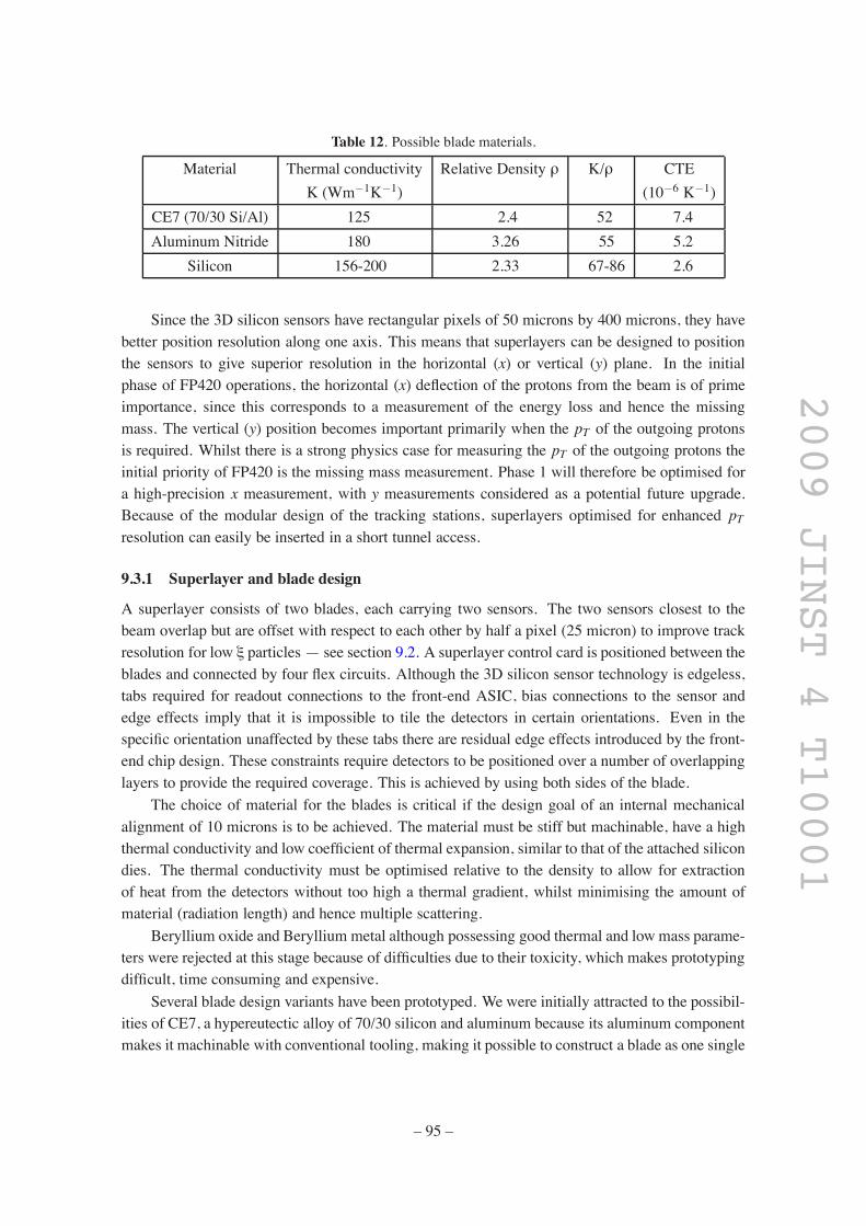
2009 JINST 4 T10001
Table 12. Possible blade materials.
Material Thermal conductivity Relative Density ρ K/ρ CTEK (Wm$1K$1) (10$6 K$1)
CE7 (70/30 Si/Al) 125 2.4 52 7.4Aluminum Nitride 180 3.26 55 5.2
Silicon 156-200 2.33 67-86 2.6
Since the 3D silicon sensors have rectangular pixels of 50 microns by 400 microns, they havebetter position resolution along one axis. This means that superlayers can be designed to positionthe sensors to give superior resolution in the horizontal (x) or vertical (y) plane. In the initialphase of FP420 operations, the horizontal (x) deflection of the protons from the beam is of primeimportance, since this corresponds to a measurement of the energy loss and hence the missingmass. The vertical (y) position becomes important primarily when the pT of the outgoing protonsis required. Whilst there is a strong physics case for measuring the pT of the outgoing protons theinitial priority of FP420 is the missing mass measurement. Phase 1 will therefore be optimised fora high-precision x measurement, with y measurements considered as a potential future upgrade.Because of the modular design of the tracking stations, superlayers optimised for enhanced pTresolution can easily be inserted in a short tunnel access.
9.3.1 Superlayer and blade design
A superlayer consists of two blades, each carrying two sensors. The two sensors closest to thebeam overlap but are offset with respect to each other by half a pixel (25 micron) to improve trackresolution for low ξ particles — see section 9.2. A superlayer control card is positioned between theblades and connected by four flex circuits. Although the 3D silicon sensor technology is edgeless,tabs required for readout connections to the front-end ASIC, bias connections to the sensor andedge effects imply that it is impossible to tile the detectors in certain orientations. Even in thespecific orientation unaffected by these tabs there are residual edge effects introduced by the front-end chip design. These constraints require detectors to be positioned over a number of overlappinglayers to provide the required coverage. This is achieved by using both sides of the blade.
The choice of material for the blades is critical if the design goal of an internal mechanicalalignment of 10 microns is to be achieved. The material must be stiff but machinable, have a highthermal conductivity and low coefficient of thermal expansion, similar to that of the attached silicondies. The thermal conductivity must be optimised relative to the density to allow for extractionof heat from the detectors without too high a thermal gradient, whilst minimising the amount ofmaterial (radiation length) and hence multiple scattering.
Beryllium oxide and Beryllium metal although possessing good thermal and lowmass parame-ters were rejected at this stage because of difficulties due to their toxicity, which makes prototypingdifficult, time consuming and expensive.
Several blade design variants have been prototyped. We were initially attracted to the possibil-ities of CE7, a hypereutectic alloy of 70/30 silicon and aluminum because its aluminum componentmakes it machinable with conventional tooling, making it possible to construct a blade as one single
– 95 –

2009 JINST 4 T10001
Figure 83. Left: A thermal model blade with the silicon resistors as described in the text. Right: Finiteelement analysis of the thermal properties of a blade.
component. Its K/ρ value of 52 compares well with more conventional materials such as aluminumnitride. The prototype blades used in the Sept 07 CERN test beam runs were of this design withthe centre sector machined down to 500 microns. However material scattering considerations arepushing the design to be even thinner — 300 microns. It has proved difficult to machine CE7 tothis tolerance due to its granular structure. Hence we have investigated an alternate design using aCE7 frame and a decoupled planar thin front section supporting the detector. This allows the use ofhard materials such as silicon or AlN whose thicknesses can be lapped down to 300 micron withhigh surface finish. The superplane shown in figure 81 has such a design. In a planar geometry therequisite shapes can be laser cut.
9.3.2 Thermal tests of the blades
Test blades have been built to investigate heat flow and thermal gradients and the resulting me-chanical displacements using a thermal camera and a “smartscope” to measure the displacement.A realistic chip/glue/support interface structure was constructed using custom silicon resistors thatmatch the size and power of the front end chip and have a similar bond pad layout. The model usedfor thermal testing is shown in figure 83. Also shown is the finite element analysis of the bladesperformed at Mullard Space Science Laboratory. The preliminary thermal tests indicate that theblade design meets the required criteria of thermal and mechanical stability at the 10 micron level.
9.3.3 Assembly and alignment
The silicon sensors will be positioned on the blades using an adaptation of the automated assemblystages and jigs used to construct silicon modules for the ATLAS SCT at Manchester. The systemuses automatic pattern recognition of fiducials on the readout chip to provide coordinates to x,y,θmotion stages which position the detector on precision jigs. Components are glued using a SonyCastPro dispensing robot under software control. The system allows silicon sensors to be reliablypositioned on opposite sides of a blade with an absolute position accuracy of 5 microns. Detector
– 96 –

2009 JINST 4 T10001
blades are independently surveyed using a Smartscope optical coordinate measuring machine ca-pable of one micron precision. Figures 84 and 85 show the build sequence for a blade and then asuperplane. Once the superplanes have been manufactured, the station needs to be assembled.
Linking individual blades together, in pairs as superlayers, and then into an entire station hassome complexities. Several approaches have been prototyped. The simplest idea is to use linkingdowel rods and precision wire cut washers stuck to each blade following the ATLAS SCT expe-rience. These can be manufactured to 5 micron tolerance. However, the alignment of a stack of10 is limited by sliding tolerances and difficulties in maintaining dowel angular tolerances. Thisled us to touch bearing designs. A touch bearing consists of a bar perpendicular to the dowel rod,pushed against it by a spring force such that there is a unique point contact between the two. Theseare arranged in a kinematic manner, providing a V and a flat. The kinematic single point contactsprovide high reproducibility, whilst the spring force allows easy movement to position along thedowel. The challenge is to make such a bearing design small enough for this application. One ofthe restrictions imposed by through dowels is that it is difficult to remove an individual superplanewithout dismantling the entire system. This leads us to our current baseline design: open-sidedtouch bearings, one V, one flat are sandwiched between two blades as part of the superplane as-sembly process. These are located against two external dowel rods, held by a small ball spring.Figure 86 shows several superplanes and their bearings without the support structure and also theminiature touch bearings.
Figure 87 shows results of repeatedly repositioning a superplane — reproducibility at the 5microns level or better is clearly demonstrated using the touch bearings. Measurements were takenusing a Smartscope optical coordinate measuring machine of fiducials on a superplane front endcompared with fixed fiducials on a base. The superplane was repeatedly removed and repositionedagainst the end bars.
To summarise: sensor to sensor positioning on a blade element can be achieved with an accu-racy of 5 microns, and within a superplane to 10 microns.
The position of any sensor in the station once built can be surveyed by the Smartscopewith a single measurement accuracy of 1 micron (several measurements may be required to linkall sensors).
9.3.4 Electrical details of the superplane
A flex circuit situated behind and bonded to the sensor is used to connect the FEC chips to thepower supply and data lines via wire bonds. The flex circuit is fitted with a control chip (the MCC)which services the FEC chips, distributing clock, control and trigger information and collectingdata for onward transmission. Aside from some slow single-ended signals, the connection betweenthe FEC and MCC chips are implemented using LVDS-style differential signaling, with lower cur-rent than LVDS terminated into 600Ω. The two-layer flex circuit is built on a 50 micron polyimidecore with a nominal track/spacing of 100 microns falling to 60 microns in the bond region, 100 mi-cron laser drilled vias, and a Ni/Au finish suitable for Al wire bonding. The flex is pre-assembled(passive decoupling components soldered) then glued to the blade. Positioning is visual with re-spect to the chip and performed with a manual placement workstation with a typical accuracy ofaround 20 microns. The positioning is not critical, the bonding process can cope with many tensof microns misplacement between flex and front end assembly. 25 micron Al wire with (99% Al,
– 97 –

2009 JINST 4 T10001
Figure 84. Blade assembly — Positioning of chips 1 to 4 on Blades A and B.
– 98 –

2009 JINST 4 T10001
Figure 85. Superplane assembly.
1% Si) is used. Wedge-wedge bonding has been undertaken with a manual (semi-automatic) wirebonder during the prototyping phase; an automatic bonder will be used in production. We planto investigate the benefits of plasma cleaning the flex, although our experience thus far has shownno difficulties bonding to the flex using a slightly elevated bonding power setting to overcome anysurface contaminants. The individual blades need to be tested before final assembly as both the sen-
– 99 –

2009 JINST 4 T10001
Figure 86. Left: Several superplanes showing the bearings without the support structure. Right: Miniaturetouch bearing. The ball bearings are 3mm diameter.
Figure 87. Superplane positioning accuracy measurement.
sor assembly and their connections on the internal faces of the blades are not accessible after theblades have been combined into a superlayer, and it would not be practical to split and repair afterassembly. The flex circuits have sacrificial tails that bring the signals to diagnostic headers. Theseconnect to adapter boards allowing connection to the ATLAS Pixel TurboDAQ system which canbe used for single chip testing. We foresee the option of potting the bonds after successful testing.Once both sides of the blade have been processed and all tests have been successfully completedthe sacrificial tails are cut away. Two blades are combined with a control card and fixed together toform a superlayer. The flex circuits are glued to the control card with solder connections betweenthe underside of the flex and the card for power, and data connections made by wire bond betweenpads on the topside of both. The bond pitch is much more generous and the alignment is not critical.The flex tension does not have any impact on the sensor positioning. The control card is a hybridbased on conventional PCB construction expected to have microvia breakout of the high density
– 100 –

2009 JINST 4 T10001
wire-bond connections to the MCC chip. Because of a shortage of MCC chips in this prototypingphase it will be necessary to mount the chip in a ceramic carrier which is placed into a socket onthe board, but final production boards will be true hybrids. The power planes of this card providethe thermal path for the heat generated by the MCC chip. The connection from the superlayer hasnot been finalised. The prototypes use a SAMTEC QTE connector that straddles the board edgeand mates to a custom made cable assembly.
Differential (LVDS like) data paths from each superlayer, together with power supply connec-tions, span the detector box assembly to the support crate positioned either inside one of the supportlegs of the NCC or in an overhead gantry nearby. At the support crate, data links are merged andpassed to the optoboard. Each superlayer has one inward link that provides clock/trigger/control,and one outward link for data. The MCC support chips offer dual output links, but because of thelow occupancy and small number of FE chips associated to each MCC (1/4 of density of the Pixeldetector) only one link is required. We hope to be able to adopt the opto-components used at AT-LAS, however the multimode fibre is susceptible to radiation which over these long distances maycause excessive attenuation, so it may be necessary to periodically replace the fibre. Alternatively,a rad-hard monomode based connection, as used at CMS, may need to be developed.
9.3.5 Station positioning
From an electrical point of view, a station is simply a collection of superlayers. It is worth notinghowever that the station is positioned inside a box that is welded to the beampipe and fitted withsubstantial lid, and so is a good Faraday cage. The blade carrier material is itself conductive; onepoint to be established therefore is whether this should be actively tied to the ground reference (thebox/ beam pipe) or left to float. RF modeling studies together with practical testing on the RF testrig at the Cockcroft institute will help to determine the optimum strategy.
The tracking station will be loosely mounted from the lid of the vacuum vessel by flexiblesupports. Services , cables and cooling feedthroughs will be on the lid.
Precision alignment with respect to the beam pipe is achieved by location with kinematic rubyball mounts on the base of the box. Figure 88 shows a station and lid, and relates these to the LHCbeam pipes. Figure 89 defines key distances that will determine how closely the active silicon willbe to the beam.
9.4 High-voltage and low-voltage power supplies
This section outlines some of the solutions envisaged for the bias and low-voltage supplies. Em-phasis is on the supplies for the 3D sensors and their front-end chips. For more details, the readeris referred to ref. [158].
9.4.1 Low-voltage power supplies specifications
Each superlayer requires two low-voltage supplies, preferably floating with minimum 1 Vcompliance range relative to each other, see table 13. The low-voltage supply for a superlayershould be floating relative to that of any other superlayer. There will be decoupling capacitorsclose to the load.
– 101 –

2009 JINST 4 T10001
Figure 88. Left: A complete tracking station attached to the lid. Also shown are the positioning studs.Right: Schematic view of the box in position around the beam pipe.
Figure 89. Key dimensions from the beam to the edge of the first chip. 1 — beam to window, 2 —window thickness, 3 — standoff of detector from window depends on thermal considerations and assemblytolerances, 4 — distance of first pixel from from edge of blade defined by dicing considerations.
Table 13. Low-voltage requirements for one ATLAS FE-I3 front-end chip. Currents are given for both 1%and 10% occupancy.
One Pixel FE-I3 chip Voltage range Nominal voltage Current Current limitAnalog AVDD 1.6-2.0 V 1.6 V 5-70 mA 100 mADigital VDD 1.5-2.5 V 2.0 V 40-50 mA (1% occ.) 100 mA
60-70 mA (10% occ.)
– 102 –

2009 JINST 4 T10001
Table 14. Supply requirement for one ATLAS MCC chip.
One MCC Voltage Current Current limitDigital VDD 1.8-2.5 V 120-150 mA 170 mA
Table 15. Overall specification for a low-voltage supply segment for one superlayer consisting of 4 Pix-elChips FE-I3 and one MCC chip. Remote monitor should enable observation of the voltage and current.
4 FE-I3 + 1 MCC Voltage range Nominal voltage Current Current limitRead-out driverAnalog (AVDD) 1.6-2.0 V 1.6 V 20-280 mA 310 mADigital (VDD) 1.8-2.5 V 2.0 V 280-350 mA (1% occ.) 480 mA
360-430 mA (10% occ.)Monitor resolution < 20 mV < 10 mA
The required digital supply current depends on the detector occupancy. High occupancy re-sults in higher current. The supply and its cables should take this into account. In table 14 therequirements for one readout controller chip MCC are listed.
As each superlayer has 4 detectors and 4 FE-I3 chips plus one MCC chip sharing the digitalsupply with the front-end, we can sum up the total requirement per superlayer as shown in table 15.
A few comments are in order. The voltages may need adjustments in the course of the lifetimeof the system due to radiation effects. The low-voltage supply may need to have remote-sense feed-back to compensate for the voltage drop. There must be a current limit which can be set either lo-cally or remotely; it would be an advantage if its value can be set remotely as this will allow a moreflexible system, capable of dealing with changes due to, for instance, radiation damage. The currentlimiting can be either of a saturating type or a fold-back with latching action. The latter requiressome means of remote reset. Currents and voltages must be monitored and results provided re-motely with the accuracy given in table 15. A sample rate of the order of 1 Hz is sufficient. It is im-portant that each superlayer low-voltage supply can be switched on/off individually (and remotely).
9.4.2 High-voltage power supplies specifications
A superlayer requires two high-voltage bias supplies, Vb1 and Vb2, with remotely controlled volt-age in the range 0 to $120 V. Vb1 and Vb2 should be floating relative to each other within asuperlayer with a compliance range on the zero terminal of at least 2 V. The high voltage bias sup-plies to a superlayer should be floating relative to any other superlayer with a similar compliancerange. As the bias voltage for depleting the detector increases with radiation damage, it is an ad-vantage to segment the supply into two: one for the detector pair closest to the beam (Vb1) and onefor the pair away from the beam (Vb2). It is not necessary to separate the ground between Vb1 andVb2 at the superlayer. The Vb zero line will be tied to the AVDD line. There will be passive RC
– 103 –

2009 JINST 4 T10001
Table 16. Specifications for the high voltage bias supplies for one superlayer consisting of four detectorspowered by two independent voltages. The voltage and current should be monitored remotely with at leastthe specified accuracy. The voltage should be controllable from remote with a resolution of better than 3 V.
4 detectors/2 voltages Voltage Current Current limitVb1 0 to $120 GeV <1 mA 1 mAVb2 0 to $120 GeV <1 mA 1 mAMonitor accuracy <1 V 1 µA # 12 bit res.Setting accuracy <3 V # 6 bit res.
Table 17. Power dissipated in the front-end electronics assuming 5 superlayers per pocket. Numbers areworst case values with 10% occupancy and maximum voltages and currents.
One superlayer Voltage (V) Current (A) Power (W)AVDD 2.0 0.28 0.56VDD 2.5 0.43 1.08Vbias1 120 0.001 0.12Vbias2 120 0.001 0.12Total per Superlayer 1.88
no of superlayersTotal per pocket 5 9.38
no of pocketsTotal per cryostat 3 28.13
low-pass filtering close to the load. Table 16 summarises the requirements.There must be a current-limit at the indicated value. To increase flexibility, it would be an
advantage if its value can be remotely adjusted. The limiting can be a simple saturating current-source type. Currents and voltages must be monitored and results provided remotely. Samplerate of the order of 1 Hz is sufficient. The high-voltage supply has to be remotely controllable.Remote-sense feedback on the wires to the load is not required as the current-induced voltage dropis negligible with respect to the required accuracy.
9.4.3 Power budget
Table 17 gives the power dissipated in the front-end for a worst case scenario where the occupancyis 10% and the voltages are at a maximum. For cooling design, the power from the radiation andthe thermal flux from the ambient will have to be added to this list.
9.4.4 Low- and high-voltage channel count
Table 18 gives the number of channels assumed. The final count may differ from this.
– 104 –

2009 JINST 4 T10001
Table 18. Number of low- and high-voltage supplies channels.
no. of channels One superlayer One pocket One cryostat FP4204 det.+ FE+1MCC with 5 superlayers with 3 pockets with 4 cryostats
Low voltage 2 10 30 120High voltage 2 10 30 120
Table 19. Preliminary specifications for the QUARTIC/GASTOF power supplies for one cryostat.
Number of channels Nominal voltage Current Current limitHigh voltage 4 $3.5 kV TBD TBDAVp12 1 12 V TBD TBDAVm12 1 $12 V TBD TBDDVp5 1 5 V TBD TBDDVp3.3 1 3.3 V TBD TBD
9.4.5 Temperature monitoring
The temperature in the front-ends needs to be monitored. It will probably be necessary to havea probe on each superlayer. Temperature sensors of NTC type are known to be radiation tolerantand are used in other detectors at LHC. For instance LHCb (VELO repeater board, Low VoltageCard) uses NTC 103KT1608-1P from Semitec. The selection of the most appropriate device willrequire a later study. It is however sure that both excitation circuitry and an ADC to read thetemperature values will be needed. It is an advantage if this excitation and measurement systemcan be integrated into the power supply crates.
9.4.6 QUARTIC/GASTOF high- and low-voltage supplies
The QUARTIC/GASTOF modules have different requirements than the 3D detectors. The specifi-cations per cryostat are for the moment rather loosely set as described in table 19.
9.4.7 Discussion of the solutions considered
All solutions discussed in the following are based on commercially available modules. Three con-ceptually different approaches have been studied.
1. Power supplies located in the tunnel next to the FP420 cryostats and stowed underneath theadjacent magnets. The advantage is the low cable cost combined with options for extensiveremote control and monitoring. The major drawback is the sensitivity to radiation, combinedwith difficult access for maintenance. A study of the radiation tolerance [159] of a solutionbased on CAEN supplies (see below) concludes that there may be 0.1 SEU (Single EventUpsets)/module/day if the modules are placed in the tunnel close to the cryostat. This will be
– 105 –

2009 JINST 4 T10001
the case from day-one of operation. This means that there will be several SEUs per day, inaddition to the damage due to dose gradually accumulating over time (tens of Grays per year).
2. Power supplies in the alcove areas RR17/13 for ATLAS and RR57/53 for CMS. Theexpected level of radiation here is 0.05-0.36 Gy/year at full LHC luminosity. This solutionis similar to that adopted for the TOTEM Roman Pots.
3. All critical power supply electronics in the counting room and only very simple linear,radiation-hard regulators in the tunnel next to the cryostat.
Except for the CAEN version of solution 1. (see below), the high-voltage supplies are alwaysassumed to be in the counting room, which is advantageous because radiation is thus no morea concern. The wires for high voltage can have a small cross section due to the small current(< 1 mA) and need no remote sense. The high-voltage cables must be well shielded and with anoise filter at the detector.
Solutions 2. and 3. with 200 m long (or longer) low-voltage cables require local regulatorsnext to the load. Without them it will not be possible to maintain a stable load voltage. Cables witha length of 200-500 m would have to have large cross section in order to limit the voltage drop tothe level required (roughly < 200 mV). Remote sensing, the classical way of overcoming this, isnot effective due to the long delay in the cable. Linear regulators, albeit with much shorter cables,are used in many LHC detector systems, such as the TOTEM Roman Pots and the LHCb VertexLocator (VELO). A pair of radiation-hard linear regulators have been developed in the frameworkof RD-49. The regulators are LHC4913 for positive voltages (SCEM: 08.57.56.011.7; 1.23 V to9 V at 3 A) and for negative voltages LHC7913-4 (SCEM: 08.57.56.111.4; $1.2 V to $7 V at3 A). In other LHC experiments using a linear regulator, a separate monitoring system for thevoltage is exploited, which has to be radiation hard. For instance, in the CMS central tracker asystem of FEC, DOHM and CCUs is used. The main issue with this solution is that it is highlyspecialised for these applications and not easily adapted to the FP420 requirements. Added to thisis the difficulty of finding the components. As an alternative solution we suggest the followingsetup, which allows remote monitoring of the load voltage (see figure 90). The voltage at the loadis fed back to the location of the power source via pairs in the same cable as the power source.We propose to put isolation resistors in series with the sense wires. As long as the ADCs at theacquisition end have high impedance and low leakage and bias current, the average current andthus the voltage drop across the sense resistors will be small. This means that the average voltagemeasured at the acquisition end will equal the average voltage at the load.
Solution 1: supplies next to the cryostat. For this configuration we have one proposal fromCAEN and two (A and B) from Wiener; all solutions still need refinements. The CAEN solutionenvisages putting both the low- and the high-voltage supplies in the tunnel; the Wiener solutionsforesee only the low-voltage supplies in the tunnel.
CAEN. The schematic layout is shown in figures 91–93.The A3006 low-voltage supply is adjustable in the 4 to 16V range and may thus not be able
to cover all the way down to 3.3 V, necessary for QUARTIC and GASTOF, without additionalmodifications.
– 106 –

2009 JINST 4 T10001
Figure 90. Block diagram showing the principle of using a local radiation-hard linear regulator. Here for apositive voltage and the option of remote monitor of the load voltage via isolation resistors Rs.
Figure 91. Solution with all supplies in the tunnel, adjacent to the cryostat. “Station” indicates the FP420cryostat and “Adj. Magn.” the magnets adjacent to the FP420 cryostat.
Figure 92. Block diagram of the CAEN setup.
Details of the degree of radiation tolerance of the CAEN modules are given in [158]. ModulesA3009, A3486, A3540, A3801 have been tested to work up to doses of about 140-150 Gy. Thefirst three are radiation-certified for ATLAS. Module A3501 has never been tested, but its radiationbehaviour should be the same as that of A3540, which has been radiation-certified for ATLAS.
The CAEN standard-module communication is not guaranteed to work over a 500 m cable.The CAEN CAN bus is operated at 250 kbit/s. A speed of 250 kbit/s has been verified to workover cable SCEM 04.21.52.140.4, without affecting signal integrity, but, due to the cable delay,the timing requirements of the CAN bus arbitration protocol are violated. Lowering the bit rate to
– 107 –

2009 JINST 4 T10001
Figure 93. Diagram of the solution suggested by CAEN. The number of pockets assumed is 3 per cryostat.Shown are also the system for temperature monitoring (A3801) and the supplies for QUARTIC/GASTOFdetectors (A3540 and A3006).
125 kbit/s would make the 500 m cable meet the specifications of signal integrity and arbitrationprotocol. CAEN has offered, at an additional cost, to modify the modules such that they operateat 125 kbit/s, but the modules will then become non-standard and will no longer be exchangeablewith those used elsewhere at CERN.
In addition, the CAEN module A3501 is designed for 0 to $100 V, whereas $120 V may benecessary, as specified above. CAEN is able to modify the modules at an additional cost.
WIENER.
Wiener, Solution A, MPOD LV next to cryostat, MPOD HV in counting room. Figures 94–95 show the schematic layout of the proposed system. This solution, based on Wiener MPODmodules, has only the low-voltage part in the tunnel. One crate at each location will be needed forthe 3D supplies. The high voltage is supplied from MPOD modules in the counting room via a500 m cable. No auxiliary power crate is needed in the tunnel, different from the CAEN solution.The MPOD modules have never been radiation tested. According to the company they are made ina way which is likely to qualify them to the level we require. It will however be necessary to testthe modules in both proton and gamma fields.
Wiener, Solution B, Maraton LV crates next to cryostat, MPOD HV in counting room. Fig-ures 96–97 show the schematic layout of the proposed system.
This solution has the low-voltage supplies housed in Wiener Maraton crates in the tunnel nextto the cryostat. One crate will be needed per pocket. The high voltage is supplied over a 500 mlong cable by an MPOD module in the counting room. This solution requires a customization ofWiener Maraton low-voltage modules in order to optimise it for low currents. The monitoring of
– 108 –
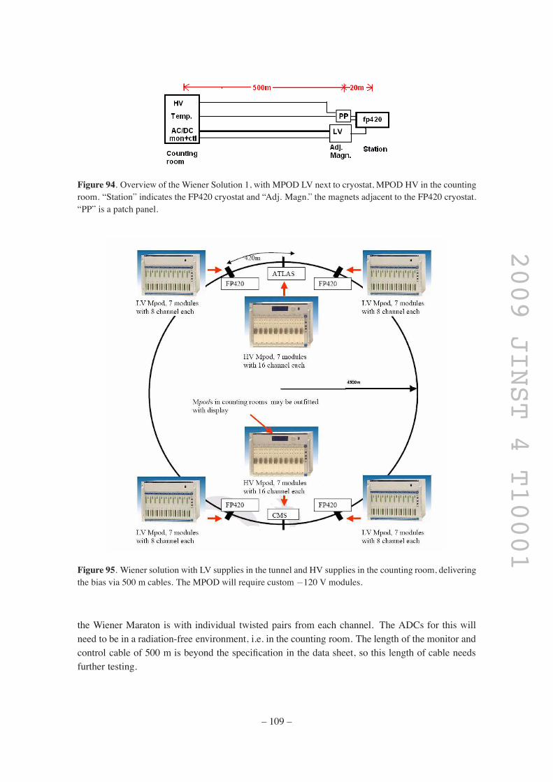
2009 JINST 4 T10001
Figure 94. Overview of the Wiener Solution 1, with MPOD LV next to cryostat, MPOD HV in the countingroom. “Station” indicates the FP420 cryostat and “Adj. Magn.” the magnets adjacent to the FP420 cryostat.“PP” is a patch panel.
Figure 95. Wiener solution with LV supplies in the tunnel and HV supplies in the counting room, deliveringthe bias via 500 m cables. The MPOD will require custom $120 V modules.
the Wiener Maraton is with individual twisted pairs from each channel. The ADCs for this willneed to be in a radiation-free environment, i.e. in the counting room. The length of the monitor andcontrol cable of 500 m is beyond the specification in the data sheet, so this length of cable needsfurther testing.
– 109 –

2009 JINST 4 T10001
Figure 96. Overview of theWiener Solution 2, based on the Maraton modules next to the cryostat. “Station”indicates the FP420 cryostat and “Adj. Magn.” the magnets adjacent to the FP420 cryostat. “PP” is a patchpanel.
Figure 97. Low-voltage Wiener Maraton supplies in the tunnel. High-voltage MPOD type supplies arelocated in the counting room. TheWienerMaraton system is qualified for the radiation environment expectedin the tunnel under the magnets near the FP420 cryostat. The illustration shows the setup for either ATLASor CMS. “Station” indicates the FP420 cryostat.
The Wiener Maraton modules have been radiation qualified to 722 Gy, and 8% 1012 n/cm2.Their good radiation tolerance is partly obtained by moving the digital part of the control andmonitoring circuitry away from the radiation zone. This results however in less flexibility comparedto the CAEN and the Wiener MPOD solutions. So in the Wiener Maraton system the output voltageand current limit cannot be adjusted from remote, and monitoring is via analogue differential wires.One pair is required per measurement value (voltage and current) resulting in a large amount ofmonitor wires. The ADCs for this will need to be in a low-radiation environment, i.e. in thecounting room. For improved radiation tolerance, mains supply AC to DC conversion is also donein the counting room.
The advantage of this solution is that it will fit the QUARTIC/GASTOF requirements withoutmuch modification. The disadvantages are the exposure to radiation and difficult access for main-tenance. In addition, the Wiener Maraton only allows the voltage setting and current limits to beadjusted manually using potentiometers on the modules. No remote tuning is possible.
– 110 –

2009 JINST 4 T10001
Figure 98. Low voltage in alcoves, rest in counting room using 200 m cables from alcove to cryostat.“Station” indicates the FP420 cryostat and “Adj. Magn.” the magnets adjacent to the FP420 cryostat. “PP”is a patch panel. “Reg” are linear regulators next to the load.
Figure 99. Low-voltage Wiener Maraton supplies in the alcoves. High-voltage MPOD supplies in thecounting room. The Wiener Maraton system is qualified for the expected radiation environment within alarge margin. “Station” indicates cryostat.
Solution 2: low-voltage supplies in alcoves, high-voltage supplies and temperature monitorin counting room, local regulators at load. This solution (figures 98–99) is based on the useof Wiener Maraton low-voltage supplies placed in the alcoves. CAEN also has radiation-tolerantpower supplies, which could be considered. TheWiener Maraton modules are used for the TOTEMRoman Pot detectors and are also placed in the alcoves.
This solution requires a customization of Wiener Maraton low-voltage modules in order tooptimise it for low currents. The length of the monitor cable of 300 m is beyond the specificationin the data sheet, so this length of cable also needs further testing, as already discussed. A linearvoltage regulator is placed next to the front-end to ensure the voltage stability at the load.
Solution 3: low- and high-voltage supplies and temperature monitor in counting room, localregulators at load. This solution is illustrated in figure 100. The advantage is that the powersupplies are not exposed to radiation. This widens the number of power supply candidates signif-icantly, lowers their cost and makes the system simpler to maintain. The major drawback is thecable cost and the need for local regulators.
– 111 –

2009 JINST 4 T10001
Figure 100. Low- and high-voltage supplies in counting room using 500 m long cables to a patch panelwith regulators next to the cryostat. “Station” indicates the FP420 cryostat and “Adj. Magn.” the magnetsadjacent to the FP420 cryostat. “PP” is a patch panel. “Reg” indicates linear regulators next to the load.
The low voltage needs to be regulated at the load as discussed earlier. The absolute maximumcable drop in the low-voltage long cables is 5.7 V. At this limit, 6 LV cables per cryostat will benecessary. Hardware tests will have to be done in order to determine if a voltage drop of 5.7 V istolerable.
9.4.8 Summary of solutions
Figure 101 summarises the solutions outlined in this section.
9.5 Readout and infrastructure at the host experiment
9.5.1 CMS and ATLAS specific issues
Readout installations at ATLAS and CMS necessarily differ, but will be based on the same parts,which are essentially single-crate versions of the ATLAS silicon readout. Refer to figure 102. Fibreconnections from the tunnel arrive at optomodules fitted to a back of crate BOC card. The BOCprovides timing adjustments and passes the data to the ROD where event segments are combinedand DSPs can perform monitoring. Event data are passed back through the BOC to an SLINKtransmitter and onward to the ATLAS standard ROS. Integration into CMS will require some mod-ification of the ROD firmware so that the output format can be interpreted as a CMS format eventstream. CMS experts describe this as “relatively straightforward”. DCS and DSS requirementshave not been studied, but again it is anticipated that these will follow the example of the existingexperiments.
9.5.2 Tracker readout and downstream data acquisition
The 3D silicon assemblies and their readout take advantage of the significant design investmentmade by the ATLAS pixel groups. The bump-bonded detector assembly mimics an ATLAS pixelelement and the downstream readout of FP420 can therefore be based very closely on the equivalentparts of the ATLAS pixel system. Each superlayer has independent connections to a support cardsituated within the support structure. LV and HV are supplied from commercial units positionednearby, as described in section 9.4. Fibre optic data links to and from the central detector areasterminate on the support cards. Each station has its own link back to a ROD card that drives eacharm of FP420. The ROD crates are easily integrated into the ATLAS readout. Integration into CMSshould require minimal work.
– 112 –
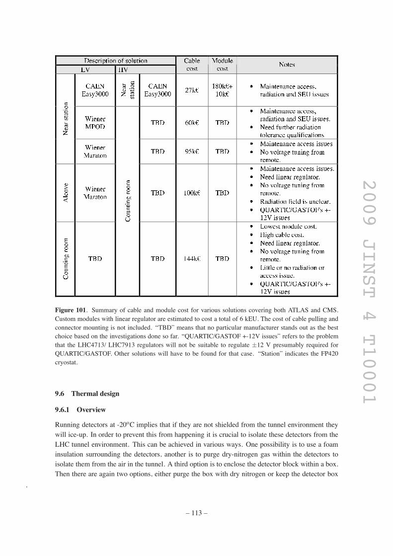
2009 JINST 4 T10001
Figure 101. Summary of cable and module cost for various solutions covering both ATLAS and CMS.Custom modules with linear regulator are estimated to cost a total of 6 kEU. The cost of cable pulling andconnector mounting is not included. “TBD” means that no particular manufacturer stands out as the bestchoice based on the investigations done so far. “QUARTIC/GASTOF +-12V issues” refers to the problemthat the LHC4713/ LHC7913 regulators will not be suitable to regulate ±12 V presumably required forQUARTIC/GASTOF. Other solutions will have to be found for that case. “Station” indicates the FP420cryostat.
9.6 Thermal design
9.6.1 Overview
Running detectors at -20oC implies that if they are not shielded from the tunnel environment theywill ice-up. In order to prevent this from happening it is crucial to isolate these detectors from theLHC tunnel environment. This can be achieved in various ways. One possibility is to use a foaminsulation surrounding the detectors, another is to purge dry-nitrogen gas within the detectors toisolate them from the air in the tunnel. A third option is to enclose the detector block within a box.Then there are again two options, either purge the box with dry nitrogen or keep the detector box
– 113 –

2009 JINST 4 T10001
Figure 102. Layout of the readout and DAQ system.
under vacuum.
1. Foam insulation is not practical within the limited available space. It would render the detec-tors themselves inaccessible (foam will have to be applied between and around the detectorplanes) and would not absolutely guarantee that no icing will take place at any point. Thismethod is considered to be cumbersome and potentially harmful to the detectors with noguarantee it will work.
2. Purging dry nitrogen gas during operation is a viable option from an engineering point ofview. However purging nitrogen gas continuously into the LHC tunnel is not allowed byCERN.
3. Maintaining a water vapour free environment around the detectors by enclosing them in abox, filled with dry nitrogen is an option. It would however compromise the cooling of thedetectors themselves due to natural convection inside the box. It would require more heat tobe pumped away compared to cooling the detectors in vacuum, which in itself is not directlyconsidered to be a show-stopper. There is however a potential for icing-up of the enclosuredue to the internal convection, which could be solved by applying heaters to the outside of theenclosure. The box would have to be gas tight, in order not to leak nitrogen into the tunnel.The convection of the nitrogen gas will yield larger thermal gradients over the detector planecompared to vacuum and potentially cause an asymmetric temperature distribution that couldaffect the measurements.
4. If the enclosure is kept under vacuum all drawbacks of option 3 disappear. Maintaininga vacuum around cold detectors is standard practice in laboratories and the technology re-quired to maintain this vacuum is bulk-standard, off the shelf. It will minimise the cooling
– 114 –

2009 JINST 4 T10001
requirements and it will minimise the thermal gradients. Maintaining a gas-tight enclosurearound the detectors (option 3) has the same level of complexity as a vacuum environment.
Option 1 is not considered to be viable and option 2 is not allowed. Because of the advantagesattached to maintaining a vacuum around the cold detectors, compared to option 3, it was decidedto go for option 4.
9.6.2 Thermal requirements
The thermal requirements for the detectors are as follows;
• Lowest allowed operating temperature is -22oC.
• Nominal operating temperature is -20oC.
• Highest allowed operating temperature is -18oC.
• Required thermal stability during operation is better than 0.5oC per 24 hours.
• The maximum allowed thermal gradient over an individual detector (chip) is 0.5oC.
• All detectors within a test setup will be operating within 2oC of each other. That is, thetemperature of the hottest detector at any given time is no more than 2oC higher than that ofthe coldest detector.
• The vacuum pipe, enclosing the LHC beam, will be at 302C ± 52C.
• The extreme temperatures to which the detectors will be exposed when non operating willbe the ambient temperature in the LHC tunnel and that during transport. These are expectedto be in the range of 102C to 402C. FP420 will not be part of the overall beam line tube bakeout.
Figure 103 illustrates how heat will be transferred from the superplanes to copper blocks in thestation support.
9.6.3 Heat loads
Heat is dissipated inside the tracker cell (mostly in the ASIC underneath) and the control card.Other than that, heat enters the detector block via thermal radiation (enclosure is sitting at 302C)and parasitic conductive heat loads via the harness and the supports. Analyses have been carriedout to size these heat loads. The results are listed in the table 104.
The dissipated heat loads are conservative estimates and make up 75% of all dissipated heat.The parasitic heat loads are best estimates at the time of writing this document. It would be prudentto put a safety factor of 2 on these numbers to quantify the required cooling power. Therefore therecommended cooling power for the cold sink should be better than 42 W. In the next sections thetemperature of the cold sink is determined.
– 115 –

2009 JINST 4 T10001
Figure 103. Front-end of a superlayer showing the cooling block arrangement.
Figure 104. The heat loads.
9.6.4 Heat flow
The heat flow/gradient is determined by the dissipated heat together with the thermal resistancebetween the source and the cold sink. The heat flow has been pictured schematically below in fig-ure 105. When the overall heat flow is known, together with the thermal resistance of the network,gradients and overall temperature differences can be determined.
The CE7 (70/30 Si/Al) plane with two tracker cells has been analysed in some detail. Simpli-fied thermal models were used to assess the effective thermal conductance between the edge andthe tracker cell. In figures 105 and 106 the overall temperature distribution for an artificial load(1 W, with boundary at 02C) is given. The resulting thermal resistance towards the edges is 1/14.3= 0.07 W/K, which assumes heat sinks on either side of the tracker planes.
– 116 –

2009 JINST 4 T10001
Figure 105. Heat flow surrounding the tracker cells (local thermal network).
Figure 106. CE7 detector plane gradient (worst-case configuration).
Figure 107 shows the gradient between the location of the tracker cells and two cold sinks oneither side (represented by two holes). One has to assume that not the whole edge of the CE7 planeis available for a thermal load path (sink), hence this worst-case approach. There are some obviousimprovements that can be made, but not many will yield a significant smaller gradient. The thermal“choke” as it were is the limited thickness of the CE7 plate, assumed here to be 300 microns.
Of interest to the sensors themselves is the gradient, in the CE7 support. This gradient isshown in figure 107.
The various thermal resistances between the actual tracker cell and the cold plate next to thedetector block have been analysed and the results are listed in the table 20.
– 117 –

2009 JINST 4 T10001
Figure 107. Gradient in the CE7 plane underneath the tracker cell (4.32C).
Table 20. Heat flow for various conductive paths.
As can be seen from table 20, the accumulated gradient between the tracker cell and the coldsink is 65.42C. In order to gain some extra margin with respect to temperature, the recommendedcooler temperature (at the heat sink) is -902C, which gives 52C margin on top of the 100% marginon the pumping capacity.
9.6.5 Cold sink
The cold sink as shown in the table above needs to sit at -902C since the tracker cell operatesat -202C nominally with a gradient of 652C down to the cold sink (and 52C extra margin). Asmentioned in the heat load section, the cold sink needs to absorb 42 W (including a safety factorof 2). This amount of heat and the gradient excludes the use of Peltier cooling devices. Peltiercooling devices are not practical when they need to bridge gradients exceeding 502C at sub-zerotemperatures. At these temperatures, Peltier devices have trouble pumping heat and they are not
– 118 –
2009 JINST 4 T10001
efficient at all (< 5%). Using Peltier coolers in stacks to bridge the gap between -902C (cold sink)and +302C (ambient) with an efficiency of less than 5% would yield the need to dump at least10kW of heat into the LHC tunnel and we would still struggle to reach the required temperatures.The alternative would be to use some kind of fluid/vapour cooling stage; however the environmentdirectly surrounding the beam line is extremely limiting. Not many cooling agents can survive theextremely intense radiation environment.
Within CERN several cooling methods have been developed. The cooling system developedfor the TOTEM project seems appropriate to cool the FP420 detectors as it has been designed and isacceptable for use in the LHC tunnel. It can reach the required cold-sink temperature with marginand has sufficient cooling power. Other options we looked into required cooling fluids with a heatexchanger but none of the cooling fluids could be guaranteed to be radiation hard. Due to symmetryconditions and in order to have at least partial redundancy in the cooling system, it would be goodto operate two coolers in parallel per detector block. Envelope restrictions or cost may howeverexclude this option.
Conclusions. The cooling system should be able to run for 2 years next to the LHC beam line,without servicing. It is strongly recommended to operate the tracker cells in vacuum. The requiredcooling for operation in vacuum is specified as follows: 42 W pumping power at -902C. There aresignificant thermal gradients predicted across the CE7 plane and underneath the tracker cell.
Recommendations. Maintain a symmetrical cooling system, following the symmetry in each de-tector plane. It will minimise gradients and provide redundancy. A cooling system by CERN asfor the TOTEM detector is recommended. The selected cooling system needs to be subjected tosignificant radiation levels during sub-system testing in preparation for the final design to proveperformance and stability. When the tracker cell design and the flexible links have matured, to-gether with the overall geometry, the analysis needs to be repeated at a slightly more detailed level.If gradients between the different super planes have to be minimised it would be prudent to intro-duce “dummy” planes at either end of the stack, sitting at the same temperature as the other planes.The extra planes would provide for a more uniform thermal radiative background.
9.7 Performance of the tracking system
The performance of the tracker has been evaluated using a simple Monte Carlo program and also bya full GEANT4 simulation. In the GEANT 4 simulation, the energy deposits within the sensitivedetector volumes are translated into elementary charges and their collection on the electrodes issimulated. Capacitative coupling between closely placed channels as well as noise contribution aretaken into account. The signal collected channel by channel is corrected by a gain factor, convertedinto an integer number and fed into a cluster-finding algorithm, if above a threshold. Clusterstypically (#90% of the cases) include just one channel. The efficiency to find at least one clusterper plane is 99.7%. A resolution on the simulated hit position close to 10µm has been measuredfor each plane. A track finding/fit algorithm based on a χ2 fit loops over the available clusters.
One feature of forward tracking that does not occur in central trackers is that the tracks have avery small angle. This means that hits in each tracking layer are highly correlated and one does notimprove the resolution by 1/
)N, where N is the number of layers. To improve matters, alternate
layers will need to be shifted by half a pixel width to improve the tracking precision.
– 119 –

2009 JINST 4 T10001
Figure 108. Angular resolution for a tracker consisting of two stations separated by 8 metres. Each layer hasa detector with a pitch of 50 microns. The curves from top to bottom are: aligned tracking layers, alternatelayers shifted by 25 microns, theoretical best result, and multiple scattering contribution. The design goal isone µrad.
This is shown using a simple Monte Carlo model in figure 108. The multiple scattering angleis roughly 2 µrad %
%
thickness/X0) per layer at 7 TeV. If each layer corresponds to about 1%of a radiation length, then one has a multiple scattering contribution of 0.2 µrad per layer. Forthe materials in this model tracker, roughly 0.2% of the protons will interact per layer. Figure 108shows calculations for a tracker consisting of N planes per station, with two stations placed 8 metresapart. The spatial precision per layer is 50 microns/ sqrt(12) = 14 micron. Shifting alternate layersby 25 micron significantly improves the tracking performance. Multiple scattering degrades thetracking resolution if the number of planes per station is increased beyond ten layers. However, tenlayers will give the design figure of one µrad.
In a full GEANT4 simulation, different layouts of the detector stations with different numbersof planes were simulated and their impact in terms of secondary interactions of 7 TeV protons wasassessed. Moreover, the impact of a middle (3rd) station was evaluated.
The secondary interaction rate (Multiple Interaction, or MI in the figures) was evaluated asthe fraction of proton tracks which have an inelastic interaction anywhere along the spectrometerbefore the last plane of the last station. It was found that in 1 mm of stainless steel, ceramic, andsilicon the secondary interaction rates are 1%, 0.5% and 0.4%, respectively. Figure 109 shows therate of secondary interactions as a function of the number of planes per station for a three-stationlayout. Contributions to the 20% rate resulting after the third station come mainly (#15%) from the1 mm ceramic support structure of the silicon detectors. Note that this is much larger than the modeltracker discussed above. The GEANT4 results led us to consider CE7, a 70%/30% Si-Al compound
– 120 –

2009 JINST 4 T10001
Figure 109. Percentage of secondary interactions (MI) as a function of the number of planes and track-ing stations. A revised design improves the performance — the two-station tracker has a 6.8% secondaryinteraction rate. See text.
support as an alternative. The contribution of a 250 µm stainless steel window, one for each station,turned out to be negligible. Consequently a more reliable secondary interaction estimate, based onan analysis of hits in the detector using realistic materials and a three-station layout is 10.1%. Fora two-station layout, this drops to 6.8%. It should be noted that if an interaction takes place in thethird station some tracks can nevertheless be well reconstructed with a χ2/NDF less than 1.5. Withthis cut, the contamination of events with secondary interactions in the signal sample is negligible— around 0.5%. Losses of events are comparable to the secondary interaction rates, and are 10.4%and 7.1% for the three- and two-station layouts respectively.
An estimate of the multiple scattering for the two- and three-station layouts is shown in fig-ure 110. Figures 111 and 112 show the χ2/NDF and angular resolution for the two-station (0.85µrad) and three-station (0.91 µrad) layouts. These are both within the design specification. Finally,the efficiency of two-track reconstruction has been found to be 86% and 80% respectively for thetwo- and three-station layouts.
– 121 –
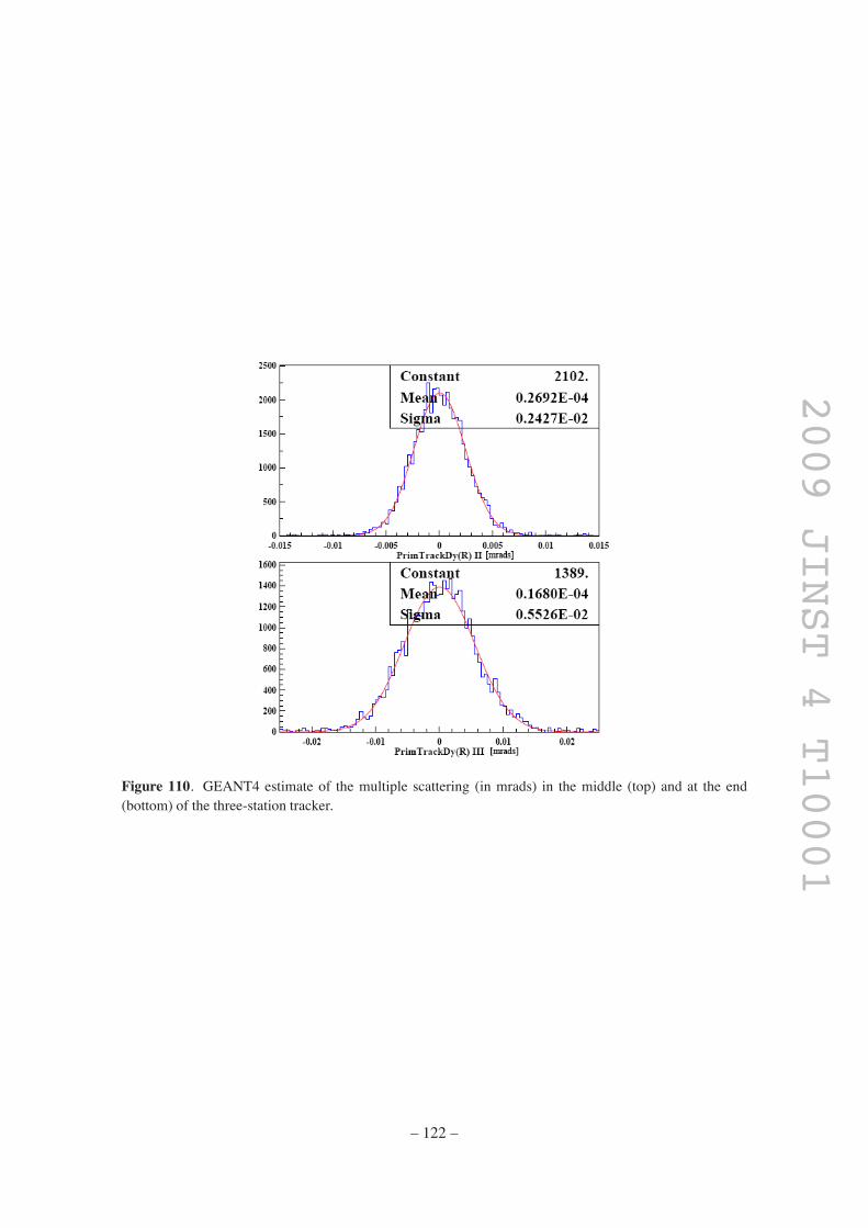
2009 JINST 4 T10001
Figure 110. GEANT4 estimate of the multiple scattering (in mrads) in the middle (top) and at the end(bottom) of the three-station tracker.
– 122 –

2009 JINST 4 T10001Figure 111. Track χ2/NDF (top) and angular resolution (bottom) for a two-station tracker. The angular
resolution is 0.85 µrad if the χ2/NDF is selected to be less than 1.5.
– 123 –
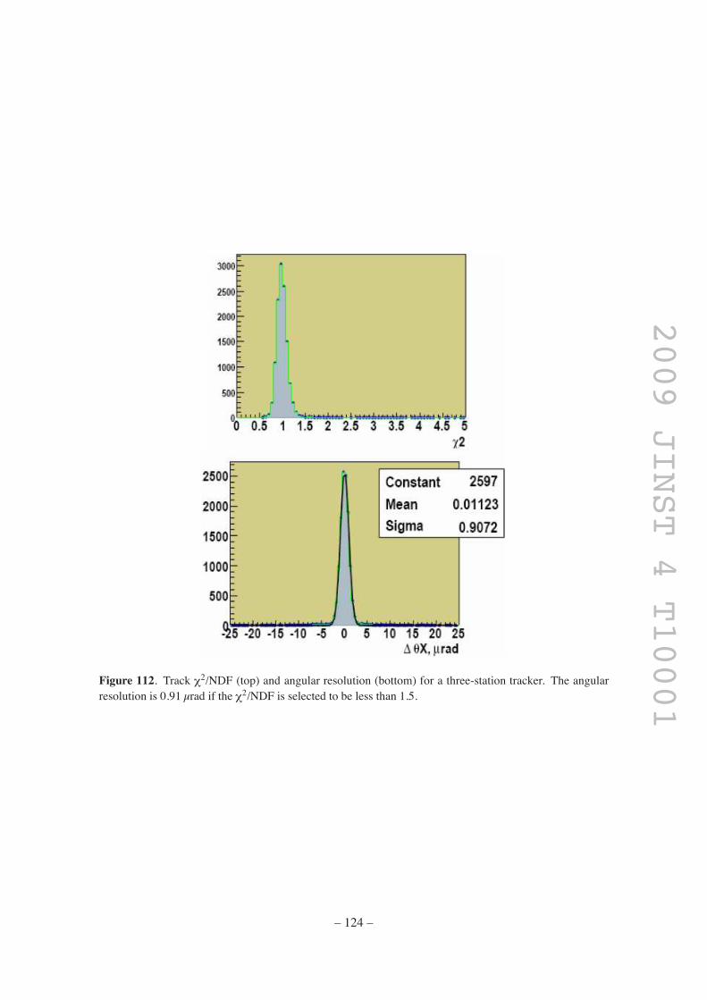
2009 JINST 4 T10001
Figure 112. Track χ2/NDF (top) and angular resolution (bottom) for a three-station tracker. The angularresolution is 0.91 µrad if the χ2/NDF is selected to be less than 1.5.
– 124 –

2009 JINST 4 T10001
Figure 113. A schematic diagram of overlap backgrounds to central exclusive production: (a) [p][X][p]:three interactions, one with a central system, and two with opposite direction single diffractive protons (b)[pp][X]: two interactions, one with a central system, and the second with two opposite direction protons (c)[p][pX]: two interactions, one with a central system and a proton, the second with a proton in the oppositedirection.
10 Fast Timing Detectors
10.1 Overlap background and kinematic constraints
The FP420 detectors must be capable of operating at the LHC design luminosity L . 1034 cm$2s$1
in order to be sensitive to femtobarn-level cross sections in the central exclusive channel [pXp]. Atthese luminosities overlap background from two single diffractive events superimposed with a cen-tral hard scatter ([p][X][p]), as shown in figure 113(a), becomes a significant concern, especiallyin dijet final states. The 2-fold overlap coincidence backgrounds, shown in figure 113(b) and (c),also must be considered, however; as they scale with L2 instead of L3 they are less of a concern inthe high luminosity limit. Fortunately, there are a number of techniques we can employ to reducethis overlap background. It can be substantially reduced at the high level trigger stage, or offline,by employing kinematic constraints. These factors, discussed in detail in the physics overlapdiscussion (section 3), include consistency between the central system and the protons in rapidityand mass, and also use the fact that the number of particle tracks associated with the event vertex ismuch smaller for exclusive than generic collisions. Even after the significant background rejectionafforded by these constraints, overlap backgrounds are still expected to dominate the signalswithout the additional rejection provided by precision timing of the protons, as detailed below.
10.2 Timing
High precision time of flight (ToF) detectors at 420 m can be used to obtain a large reduction inoverlap (or pile-up) backgrounds [1]. We need only measure the relative arrival time of the twoprotons, Δt = tL$ tR. Under the assumption that they originate from the same event, the z-positionof that event can be calculated as zpp = 1
2Δt%c. The uncertainty on zpp is δzpp = c)2δt, where δt is
the (r.m.s.) time resolution of the proton measurement. For example, δt = 10 ps implies δzpp = 2.1mm. We then require a match between zpp and the vertex position from the central detector, zvertex,which is known with extremely good precision (. 50 µm) [160].
In the case of the overlap backgrounds, the protons do not originate from the same event asthe hard scatter and so the vertex reconstructed from time-of-flight information will, in general,not match the vertex observed in the central detector, which implies that a large rejection factorcan be obtained. This rejection factor depends on four parameters; the timing resolution δt, thespread in interaction points σz, the vertex window size (i.e. the degree to which the vertices arerequired to match) and the luminosity. As the luminosity increases, the probability of there being
– 125 –

2009 JINST 4 T10001
more than one proton in an arm of FP420 increases. If any of the subsequent timing measurementsresults in a vertex that coincides with the central vertex, then these protons would be chosen asthe ‘correct’ protons. Hence the rejection factor degrades slightly with increasing luminosity. Thevertex window size is a trade-off between high signal efficiency and high background rejection.Clearly a smaller vertex window results in a higher background rejection but will also lead to moresignal events failing the vertex matching requirement. Common choices are that the vertices mustcoincide to within 1, 1.5 or 2%δzpp, which corresponds to a signal efficiency of 68%, 87% and95% respectively. Finally, the rejection factor increases if the spread in vertices increases and isalso approximately linear with δt.
The prototype detectors described below have a timing resolution of δt / 20 ps. As the lu-minosity grows, better timing resolution is required. We envisage a program of detector upgradesto match this requirement, eventually attaining resolutions smaller than 10 ps, as discussed in sec-tion 10.9. The relatively small and inexpensive precision ToF detectors discussed here make thisapproach viable.
We have calculated the background rejection for the three overlap cases shown in figure 113(a) [p][p][X] (b) [pp][X] and (c) [pX][p]. For example, if δt = 20 ps (δzpp = 4.2 mm) and thespread in interaction points is σz . 50 mm [160], we obtain a rejection factor of 21 for the first twocases and 15 for the third if the vertex measurement from proton time-of-flight is required to fallwithin ±4.2 mm (±1% δzpp) of the vertex measured by the central detector. Case (a) dominatesat high luminosity and consequently for δt = 10 ps, we would be able to obtain a rejection factorof greater than 40 (for a ±1% δzpp vertex window), enabling FP420 to effectively cope with thelarge overlap backgrounds at the design luminosity. Note that the rejection factors presented intable 8 in section 3.3 are smaller than those presented here due to a larger vertex window (±2δzpp),which maximises the signal efficiency, and also a narrower spread in interaction points of 44.5 mm.This pessimistic vertex distribution is based on a large crossing angle scenario and results in areduced background suppression power using the ToF detectors. For the nominal crossing angleof 250 µrad, the vertex spread exceeds 5 cm, and in addition, the expected growth in σz wouldresult in an improved rejection. The final choice of vertex window will be optimised based on theanalysis goals and instantaneous luminosity. For example, a discovery measurement would likelymaximize signal to background, while a measurement of a state’s properties, might demand verylow background at the expense of signal efficiency.
In addition to detector performance, there are other factors that could impact the overall tim-ing precision. If the path length of protons detected in FP420 were to vary significantly, this coulddegrade the vertex measurement accuracy. We have determined that even for the largest energyloss for protons in our acceptance compared to the beam protons, the path difference amounts toless than 30 µm, corresponding to a 100 fs time difference (an even smaller effect is expected fromproton velocity differences). A second concern is that a precise measurement of the arrival time dif-ference between deflected protons in the ToF detectors requires a reference timing signal at each de-tector with a tL$ tR jitter that is small enough not to contribute significantly to the overall time reso-lution. The large ToF detector separation of about 850 mmakes this a challenging requirement. Ourreference timing system, designed to yield an r.m.s. jitter of σLR. 5 ps, is described in section 10.7.
The absolute calibration of the ToF detectors z-coordinate measurement will be determinedand monitored with double pomeron exchange (DPE) physics events to correlate the vertex position
– 126 –

2009 JINST 4 T10001
measured with the central trackers with the vertex measured by the FP420 timing detectors. Sinceit is not possible to trigger on the protons at Level-1, it will be necessary to add a double pomeronfilter at the High-Level-Trigger to the highest cross section candidate DPE processes that pass theLevel-1 trigger, dijets and dileptons, for example, to select an adequate sample of events. Giventhe high cross section for DPE dijets (1.2 nb for ET > 50 GeV, see table 7), it will be possible tocollect hundreds of such events per hour.
10.3 Timing detectors
For quite a while the standard for time of flight detectors has been in the 100 ps range. Recently,there has been an explosion of interest in fast timing for medical purposes in addition to highenergy physics detectors, and the idea of a detector with a few ps resolution is no longer consid-ered unreasonable [161]. The ALICE collaboration has developed a time of flight system that hasachieved a time resolution of about 20 ps [162]. A time resolution of σ = 6.2 ps (with σ . 30 psfor a single photoelectron) was recently achieved by a group from Nagoya [163] utilizing promptCerenkov radiation. A beam of 3 GeV/c pions was passed through a quartz radiator in line witha micro-channel plate photomultiplier tube (MCP-PMT). MCP-PMTs consist of a quartz faceplateand a photocathode followed by two back-to-back chevroned microchannel plates read out by asingle anode or multi-anode pads. They are compact (only about 3 cm in depth) and provide again of about 106 for a typical operating voltage of 2.5 to 3.0 kV. Our requirements of an edgelessdetector to measure particles within several mm of the beam combined with the very high beamenergy renders the Nagoya geometry unusable, but alternate detector concepts described below arelikely to be capable of 10 ps or better resolution.
Three main factors affect the time resolution of Cerenkov detectors: (1) the spread in arrivaltime of photons at the photocathode, (2) the time resolution of the MCP-PMT, dominated by thetransit time spread (TTS) of the electrons from emission at the photocathode to arrival at the an-odes, and (3) the downstream electronics, including signal dispersion in cables. The first factoris minimised using Cerenkov light and optimised geometrical designs. The MCP-PMTs we areconsidering have a small TTS, about 30 ps for a single photoelectron, or better, leading to a resolu-tion of 30 ps/)npe. The major manufacturers of MCP-PMTs are Hamamatsu [164], Photek [165],and Photonis [166]. Hamamatsu and Photek have concentrated on single channel tubes typicallyof small active area (11 mm diameter), for which the TTS may be as low as approximately 15 ps.Photonis’ tubes are larger (48 mm % 48 mm) and include a 64 pixel version that is well matched toone of our detector concepts.
We are developing two types of ToF counters for FP420, GASTOF (Gas Time Of Flight)and QUARTIC (QUARtz TIming Cerenkov). Prototypes of both types of detector have been builtand tested.
A schematic diagram of the GASTOF detector developed at UC Louvain is shown in fig-ure 114. It has a gas radiator at 1.1–1.4 bar in a rectangular box of 20–30 cm length, with a verythin wall adjacent to a specially designed flat pocket in the Hamburg beam pipe (section 7). Theprotons are all essentially parallel to the axis. A thin 452 concave mirror at the back reflects thelight to a MCP-PMT. The gas used in the tests, and which we propose to use in FP420, is C4F10,which is non-toxic and non-flammable, and has a refractive index n= 1.0014 between 200 nm and
– 127 –

2009 JINST 4 T10001
Proton
MCP-PMT
Lens
MirrorCerenkov gas
30 cm
Aluminium pump
10 cm
gastof™
Figure 114. Schematic of GASTOF, a gas-based Cerenkov counter proposed by Louvain-la-Neuve, asdescribed in the text.
650 nm, giving a Cerenkov angle (β = 1) of about 3.02. C4F10 is used in the RICH1 detector of theLHCb experiment.
The in-line material in a GASTOF (thin windows, mirror and gas) is minimal and does notcause significant multiple scattering. It can therefore be placed before the final tracking detectors.The GASTOF is intrinsically radiation hard, the only sensitive element being the MCP-PMT. Life-time tests on gain, transit time spread, and quantum efficiency under laser light irradiation werecarried out on Hamamatsu and Budker Institute tubes by the Nagoya group [167]. At 2.8%1014
photons/cm2 some gain decrease occurred, recoverable by increasing the HV, but the TTS was notaffected. However, a significant deterioration of the photocathode quantum efficiency (QE) wasobserved. Such an effect could be remedied by increasing the gas pressure and thus the number ofCerenkov photons — for a 30 cm GASTOF and the nominal QE, the mean number of photoelec-trons can well exceed 10.
The QUARTIC detector, which utilises fused silica (artificial quartz) bars as radiators, is beingdeveloped by the University of Alberta, Fermilab, and the University of Texas, Arlington andLouvain-la-Neuve groups. Figure 115(a) shows the concept: a proton passing through the silicabars radiates photons which are measured by the MCP-PMT. Figure 115(b) shows the 4 % 8 arrayof bars with a 6 mm % 6 mm cross section and length ranging from about 110 mm for the first barhit by the proton to 70 mm for the last, and will be flush with the surface of the MCP-PMT. Thebars are oriented at the average Cerenkov angle, θc . 482, which serves to minimise the numberof reflections as the light propagates to the MCP-PMT. Figure 115(c) shows a third generationsingle-row prototype used in the June 2008 CERN test beam. The final four-row version will havea very thin wall adjacent to the beam pipe, matching the dead area of the silicon detectors, to ensurefull acceptance for all measured tracks. It will also use short tapered aluminised air light guides tochannel the light into the respective pixels of the MCP-PMT.
Since the GASTOF and QUARTIC detectors have complementary features as discussed below,we are proposing to use both: one GASTOF detector will be located in its own beam pipe pocket
– 128 –

2009 JINST 4 T10001
proton
phot
ons
(a)
(b) (c)
Figure 115. Conceptual drawings of a QUARTIC detector, (a) showing the proton passing through eight barsof one row in x providing eight measurements of the proton time (b) showing the 4%8 layout of QUARTICbars (c) A photograph of the prototype detector used in the June 2008 CERN test beam.
after the first silicon detector pocket and two QUARTIC detectors will be located in their ownpocket after the final silicon tracking detector, to mitigate the impact of multiple scattering.
10.4 Detector simulations
Ray tracing and GEANT4 simulations of the propagation, absorption, reflection, and arrival time (atthe MCP-PMT face) of Cerenkov photons have been performed using the GASTOF and QUARTICdetector designs. These simulations provide an important aid to our understanding of the proposeddetectors.
Figure 116(a) shows GEANT simulation results for the distribution of arrival time of photonsat the MCP-PMT face for a 30 cm long GASTOF.Due to GASTOF’s optimised geometry and smallCerenkov angle all the photons arrive within a few picoseconds, consequently the time resolutionis dominated by transit time jitter in the MCP-PMT and the subsequent electronics.
Figure 116(b) shows simulation results for the distribution of arrival time of photons for a 90mm long QUARTIC bar. For the QUARTIC bar the bulk of the photoelectrons arrive within 40 ps,and there is a long tail to much larger times. The width of the peak is due to the time dispersionfrom the wavelength dependence of the index of refraction in silica, while the long tail is dueto photons emitted at different azimuthal angles, which leads to a variable path length. Both theGASTOF and the QUARTIC simulations show an expected yield after quantum efficiency of about
– 129 –

2009 JINST 4 T10001
(a) (b)
Figure 116. Simulated time of arrival of Cerenkov photons at the MCP-PMT photocathode for (a) GASTOF(b) QUARTIC.
10 photoelectrons. Although the time spread for a QUARTIC bar is much larger than the GASTOF,the philosophy of the QUARTIC detector is to compensate for the inferior resolution of a singlechannel by performing multiple measurements. A proton traverses eight bars in each of the twoQUARTIC detectors, giving 16 measurements with up to a 4-fold improvement in resolution overthat of a single bar. The QUARTIC detector also has x-segmentation that will be useful to timemultiple protons in the same bunch crossing.
Ideas for combining the advantages of the two detectors to yield a segmented detector withsuperior resolution for 2012 are being pursued and are discussed in section 10.9.
10.5 Performance in test-beam measurements
Test beam measurements over the last few years have validated the detector concepts. Two of thetest beam runs, March 2007 at Fermilab and June 2008 at CERN were particularly successful andsome of the results are reported here.
In the March 2007 test-beam we used a 120 GeV proton beam to test two GASTOFs, G1 andG2, and several 15 mm long QUARTIC bars. G1 was an initial prototype which ganged togetherfour central channels of the (8% 8 array of 6 mm % 6 mm pixels) Burle 85011-501 MCP-PMTwith 25 µm pores. G2 was a second-generation prototype using an 11 mm diameter single channelHamamatsu R3809U-50 MCP-PMTwith 6 µm pores. The QUARTIC detector used a Burle 85011-501 with 10 µm pores. The signal for the MCP-PMT’s was amplified using a GHz amplifier, passedthrough a constant fraction discriminator (CFD), and read out by a Phillips 7186 TDC. Severaltypes of amplifiers were tested: ORTEC 9306, Phillips BGA2712, Hamamatsu C5594, and Mini-Circuits ZX60-14012L. Several different CFD’s were also used: ORTEC 934, ORTEC 9307, and aLouvain-made CFD circuit (LCFD). We used a CAMAC-based data-acquisition system triggeredby scintillator tiles located on either end of the detector setup. Multiwire proportional chambersprovided track position information.
While the data-acquisition system provided a wealth of data allowing us to compare the per-formance of the different components and multiple channels, the most useful results for evaluatingthe detector performance were derived from an analysis of waveforms recorded from four channels
– 130 –

2009 JINST 4 T10001
Figure 117. The time difference between the first (G1) and second generation (G2) GASTOF prototypedetectors from the March 2007 test beam.
(G1, G2, Q1 and Q4) using a Tektronix DPO70404 4 GHz digital oscilloscope. Offline we appliedfixed threshold discrimination and constant fraction discrimination algorithms.
Figure 117 shows the time difference between the two GASTOF detectors, with δt(G1$G2)= 35±1 ps (r.m.s.). If the two detectors were identical this would imply a 25 ps resolution foreach. The G2 detector is superior to G1, however, due to an improved design resulting in a largernumber of photoelectrons, and the use of the 6 µm pore Hamamatsu MCP-PMT resulting in areduced transit time jitter. From the time differences between all pairs of channels we infer theindividual resolutions obtaining δt(G1) = 32 ps and δt(G2) = 13 ps. The G2 detector is expected tobe superior due to a better mirror and a faster MCP-PMT. Unfolding the resolutions of QUARTICbars, we find δt . 60 ps for the 15 mm long bars. The G1 efficiency was measured to be about# 98%, while the G2 and QUARTIC bar efficiencies were measured to be about 80%, but due tolimited statistics and concerns about the tracking alignment, we repeated these measurements inthe subsequent June 2008 test beam.
The June 2008 test beam at CERN used a beam of 180 GeV pions with the same GASTOF de-tectors as the Fermilab test beam, but a new QUARTIC prototype that had 90 mm long bars. Mini-Circuit amplifiers were used, with and without the LCFD. LeCroy 7300 and 8620 oscilloscopes, 3and 6 GHz respectively, were used in segmented memory mode for the data acquisition. Prelimi-nary measurements of the oscilloscope data confirm that the G2 resolution is 13 to 15 ps. A siliconstrip tracking system with 50 µm pitch was used to provide tracking information. The trigger forthe silicon telescope was used also to trigger the oscilloscopes for some portion of the data, allow-ing synchronization of the tracking readout with the oscilloscopes. The tracking allowed a detailedstudy of the efficiency as a function of position, yielding an efficiency measurement of about 90%near the edge of the GASTOF detector rising over a few mm to 99% at the center of the detector.
During this test beam, signals from several of the long QUARTIC bars were passed through
– 131 –

2009 JINST 4 T10001
Figure 118. The time difference between two 90 mm long QUARTIC bars as described in text.
the LCFD, and the resulting NIM pulses were recorded with the LeCroy 8620a oscilloscope. Fig-ure 118 shows the time difference between two of the long QUARTIC bars, with δt(Q1$Q2) = 56ps (r.m.s.). This implies a QUARTIC bar resolution of 40 ps including the LCFD. Measurements ofthe LCFD resolution alone give about 25 ps, implying an intrinsic bar resolution of 30 ps. Prelim-inary studies show a uniform efficiency of near 90% across the bar. It is likely possible to increasethe efficiency, by lowering the threshold of the constant fraction discriminator, and such studies arein progress using the raw waveforms. Given a 90% efficiency we would expect about 14 measure-ments per event for two 8-bar QUARTIC detectors, implying an overall resolution of about 11 psfor the QUARTIC detectors alone, including the effect of a 20 ps TDC.14 This
)N dependence
must still be demonstrated using a full detector row with the final detector and TDC system.The single-channel GASTOF detector has an intrinsic detector/MCP-PMT resolution on the
order of 10 ps, so requires a different electronics strategy to maintain this superior resolution. Asdiscussed in the next section, we envisage using a single photon counter with fast oscilloscopetechnology to maintain an overall timing resolution of 15 ps or better, even without further im-provements, such as offline corrections to position of the tracks through the detector (which will beknown to σ(x,y) . 5 µm).
10.6 Electronics and data acquisition
The fast readout electronics must provide a timing resolution compatible with the baseline designof the ToF detectors. The Alberta and Louvain groups have extensive experience in this area and areresponsible for the design and prototyping of the readout electronics. Both groups have developedfast amplifier boards and CFD boards for use in the beam tests. Independent tests with a fastlaser have verified that the performance of these boards is comparable to commercial units, but thecustom boards have the advantages of being much more compact and less expensive.
14Recent beam tests at Fermilab (June 2009) demonstrated σ(t) = 18 ps for a 2-bar, 2 MCP-PMT QUARTIC detector.
– 132 –
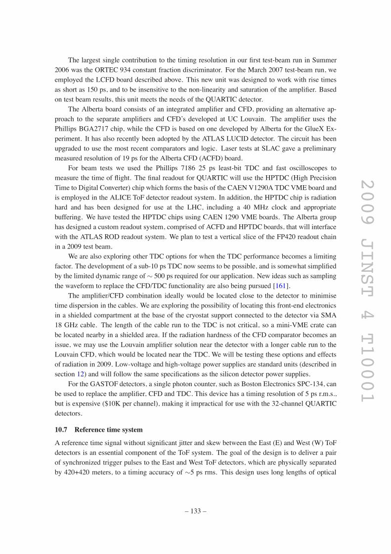
2009 JINST 4 T10001
The largest single contribution to the timing resolution in our first test-beam run in Summer2006 was the ORTEC 934 constant fraction discriminator. For the March 2007 test-beam run, weemployed the LCFD board described above. This new unit was designed to work with rise timesas short as 150 ps, and to be insensitive to the non-linearity and saturation of the amplifier. Basedon test beam results, this unit meets the needs of the QUARTIC detector.
The Alberta board consists of an integrated amplifier and CFD, providing an alternative ap-proach to the separate amplifiers and CFD’s developed at UC Louvain. The amplifier uses thePhillips BGA2717 chip, while the CFD is based on one developed by Alberta for the GlueX Ex-periment. It has also recently been adopted by the ATLAS LUCID detector. The circuit has beenupgraded to use the most recent comparators and logic. Laser tests at SLAC gave a preliminarymeasured resolution of 19 ps for the Alberta CFD (ACFD) board.
For beam tests we used the Phillips 7186 25 ps least-bit TDC and fast oscilloscopes tomeasure the time of flight. The final readout for QUARTIC will use the HPTDC (High PrecisionTime to Digital Converter) chip which forms the basis of the CAEN V1290A TDC VME board andis employed in the ALICE ToF detector readout system. In addition, the HPTDC chip is radiationhard and has been designed for use at the LHC, including a 40 MHz clock and appropriatebuffering. We have tested the HPTDC chips using CAEN 1290 VME boards. The Alberta grouphas designed a custom readout system, comprised of ACFD and HPTDC boards, that will interfacewith the ATLAS ROD readout system. We plan to test a vertical slice of the FP420 readout chainin a 2009 test beam.
We are also exploring other TDC options for when the TDC performance becomes a limitingfactor. The development of a sub-10 ps TDC now seems to be possible, and is somewhat simplifiedby the limited dynamic range of# 500 ps required for our application. New ideas such as samplingthe waveform to replace the CFD/TDC functionality are also being pursued [161].
The amplifier/CFD combination ideally would be located close to the detector to minimisetime dispersion in the cables. We are exploring the possibility of locating this front-end electronicsin a shielded compartment at the base of the cryostat support connected to the detector via SMA18 GHz cable. The length of the cable run to the TDC is not critical, so a mini-VME crate canbe located nearby in a shielded area. If the radiation hardness of the CFD comparator becomes anissue, we may use the Louvain amplifier solution near the detector with a longer cable run to theLouvain CFD, which would be located near the TDC. We will be testing these options and effectsof radiation in 2009. Low-voltage and high-voltage power supplies are standard units (described insection 12) and will follow the same specifications as the silicon detector power supplies.
For the GASTOF detectors, a single photon counter, such as Boston Electronics SPC-134, canbe used to replace the amplifier, CFD and TDC. This device has a timing resolution of 5 ps r.m.s.,but is expensive ($10K per channel), making it impractical for use with the 32-channel QUARTICdetectors.
10.7 Reference time system
A reference time signal without significant jitter and skew between the East (E) and West (W) ToFdetectors is an essential component of the ToF system. The goal of the design is to deliver a pairof synchronized trigger pulses to the East and West ToF detectors, which are physically separatedby 420+420 meters, to a timing accuracy of #5 ps rms. This design uses long lengths of optical
– 133 –

2009 JINST 4 T10001
fibers to deliver pairs of low timing jitter trigger pulses to both ToF detectors. To minimize modaland group velocity dispersions, single-mode communication optical fibers and reliable industrial10-Gbit Ethernet optical backbone components operating at the wavelength of 1.3 µm are used.
We rely on the high stability master bunch clock at CERN to derive our reference timingsystem. This master bunch clock is frequency divided by 10 from the 400 MHz superconductingRF cavity frequency. The divider is synchronized to the revolution frequency. The delay betweenthe edge of the master bunch clock and the passage of a bunch is fixed from beam run to run. Thismaster bunch clock is a stable constant frequency square wave at 40.078879 MHz with a stabilityof 50 ppm corresponding to 1.25 ps phase variation. Although this encoded bunch clock signal isbroadcast by the Timing Trigger and Control (TTC) transmitters around the CERN complex viasingle mode fibers (1.31 µm) to various LHC instrumentation and experiment areas, to minimizethe added timing jitter and skew we design our reference time system starting at the stabilized40.078879 MHz reference electrical square pulse.
A block diagram depicting the various elements of this system is shown in figure 119. A stablesignal pulse is derived from the 40.078879 MHz bunch clock provided by the LHC TTC system.15
This RF signal is received by a programmable TTC receiver and to provide programmablepost-skewing or de-skewing of the clock period in steps of 104 ps. Because the coincident RFtrigger pulse arrives #700 ns later than the proton-proton interaction, the post-skewing featureallows the triggers for the ToF detectors to be associated with the corresponding bunch crossings.
A time drift between both arms is expected to be dominated by environmental effects, primar-ily caused by the long length of 420 meter single-mode fibers. Based on the thermal optical coeffi-cient (dn/dT ) of#1.28%10$5/oC and the thermal expansion coefficient (dl/dT ) of#5.5%10$5/oCfor typical communication optical fibers, a total time drift of #20 ps/oC is anticipated for a #420meter long single-mode fiber. Hence, all fibers and optoelectronics need to be housed in a temper-ature stabilized environment.
This 40 MHz electrical pulse is converted to 1.3 µm optical pulse through an E/O converter.This E/O converter can be a 1.3 µm single-mode Vertical cavity surface emitting laser (Vcsel)based optical front end driver for the 10 Gbit/s (IEEE 802.3ae standard) Ethernet transceiver whichhas a low timing jitter of 10 ps peak-to-peak (such as Finisar FTLX1411D3). A typical 10-Gbit/sreturn-to-zero optical pulse has a width of #100 ps with a rise-time of #20 ps and a peak opticalpower of 2 mW containing #106 photons/pulse. The optical pulse is then split to two replica in anon-polarization single-mode 2%2 splitter and sent along each of the#420 meter long single-modefibers to both East and West ToF detector stations. At each end of the optical fiber, the light pulse isfurther split to two, one to trigger the stop of the Time-to-Digital Converter (TDC), while the otheris fiber butt-coupled to a Faraday mirror and retro-reflected back to the source point through the2%2 splitter. The returned pulse typically contains #105 photons/pulse and is fiber-coupled to anoptical correlator or an optical oscilloscope. At the input end of the optical correlator an amplifiedfast photodiode or a single-photon detector convert the optical pulses and are displayed on anelectronic sampling oscilloscope with a time resolution of <5 ps. Alternatively, a 500 GHz opticalsampling oscilloscope (Alnair Labs Eye-Checker) can be used which has temporal resolution of<2 ps and a timing jitter of <0.1 ps. The time different between the rising edges of the two pulses
15We thank S.Baron and Jan Troska for information and design work.
– 134 –

2009 JINST 4 T10001
Figure 119. A schematic of the reference time system. Components labeled in black are expected tocome from CERN TTC system, components labeled in blue are associated with the ToF detectors, and thecomponents in red (highlighted in the yellow box) are the optical components related to the reference timingsystem.
δtre f retro-reflected from both arms is used as a feedback signal to drive a free-space delay scanstage deployed on one arm (West) of the #420 meter long optical path. The error signal from δtre fis automatically adjusted to less than <5 ps rms (1.5 mm free space) for every bunch crossing.Prior to trigger the TDC, an Optical Constant Fraction Discriminator (OCFD), such as OFC-401, isused to suppress the electronic trigger delay shifts due to optical signal pulse amplitude variation.With this reference timing system, the two path of the trigger pulse for the ToF detectors can besynchronized to an absolute time difference of <5 ps rms. It is worth to note that this opticalreference timing system is used to compensate mostly the slow environmental drift on the twoarms of the trigger system.
10.8 Central detector timing
To this point, we have been focussing on relative timing of the forward protons to provide a vertexposition measurement for comparison with the position of the central vertex. In ref. [168] thespace-time distribution of the luminosity profile for design beam parameters was calculated, andit was found that the position and time distributions of the vertex factorise. This implies that anabsolute timing of the central detector portion of the event (two 60 GeV b-quark jets, for example)
– 135 –

2009 JINST 4 T10001
to significantly better than # 100 ps would in principle provide a further overlap reduction factorfor [p][X][p] events discussed earlier.
From test-beam results the ATLAS Electromagnetic Calorimeter (ECAL) was found to have anoise term of 500 ps/E(GeV) and a constant term of 70 ps. Similar test-beam results were obtainedby the CMS ECAL. Reductions in the clock jitter could result in a smaller constant term duringstandard data taking. We have begun simulations to determine what central detector time resolutionis possible for ATLAS and CMS. A 70 ps event resolution already would provide an additionalfactor of two in overlap rejection, and if it is eventually possible to reduce this to 10 ps this factorgrows to 12.
10.9 Timing summary and future plans
We are in the process of developing an ultra-fast TOF detector system which will have a key rolein the FP420 project by helping to reject overlap background that can fake our signal. Tests ofthe current prototype detector design imply an initial detector resolution of δt / 20 ps, includingthe full electronics chain, with an upgrade path to resolutions better than 10 ps matching the needfor improved rejection as the luminosity increases. For a luminosity of L . 21033 cm$2s$1, a30 ps detector would be sufficient to keep the overlap background to the level of other backgroundsfor the dijet channels, and render it negligible for other final states. For L . 51033 cm$2s$1, a10 ps detector (still with loose vertex cuts to maximise signal efficiency) would be desirable to keepoverlap backgrounds totally under control, without any loss in signal efficiency. For L . 71033–1034 cm$2s$1 to the design luminosity, we would control the background by (i) developing timingdetectors in the 5 ps range, or (ii) adding extra rejection from central timing, or (iii) tightening thevertex window or other background cuts (a factor of several in rejection is possible with a modestloss of efficiency), or more likely a combination of all of the above.
In addition to further analysis and beam tests to fully evaluate the current prototypes, weare continuing a program of simulation, development and testing of the detector concepts andelectronics to provide a fully optimised robust timing solution. The simplest approach to achievingfaster timing is in upgrades to the existing detectors. Further optimisation is possible throughadvances in MCP-PMT technology. The transit time spread of the MCP-PMT dominates theGASTOF resolution, so a pore size of 3 µm (offered by Photek) would already be expected toyield a time resolution better than 10 ps. For the QUARTIC detector a next generation MCP-PMTwith smaller pixel sizes would allow finer x segmentation for improved multi-proton timing. Asmaller pore size would not be expected to dramatically improve the time resolution, since thelargest component is the intrinsic detector resolution, but might yield modest improvements on the10-20% level. Better electronics could also give an improvement, with the combination resultingin a sub 10 ps QUARTIC detector as well.
Each arm of FP420 will only contain three MCP-PMTs (in the present baseline design) and,unlike the central detectors elements, they could simply be replaced every long shutdown if neces-sary. The mechanical design will allow for quick replacement.
At maximum luminosity the proposed detectors will have rates in the 10 MHz range andsee an integrated charge of a few to tens of coulombs per year depending on the exact detailsof the detectors and the gain at which the phototubes are operated. The current commerciallyavailable MCP-PMT’s will not sustain such high rates and will not have an adequate lifetime. We
– 136 –

2009 JINST 4 T10001
are pursuing developments with the phototube vendors to address these issues. There are many rateand lifetime improvement proposals in various stages of development that will improve the rate andlifetime capabilities of these phototubes, including an increased pore angle to reduce ions strikingand damaging the photo-cathode, adding a thin aluminum film at the front face or between thetwo microchannel plates to suppress the back-scattered ions, gating the cathode during dead-timeperiods, and new photocathode and MCP materials. We plan to make our own rate and lifetimemeasurements using newly operational laser test stands at UC-Louvain and UT-Arlington. TheUCL group has already demonstrated that they can successfully operate the GASTOF with theHamamatsu tube at a gain at least five times lower than the standard 106 gain (reducing boththe lifetime and rate issues), and similar studies are in progress at UTA for the Photonis tubes.We anticipate that the GASTOF detectors will be able to operate to intermediate luminosities L. 2% 1033 cm$2s$1, with little or no improvements to the MCP-PMT’s, while the QUARTICdetectors likely need modest MCP-PMT improvements to survive Phase I (intermediate luminosity)operations. In order to have satisfactory performance under Phase II (high luminosity) conditions,upgrades will be needed to both improve the timing resolution of the detectors and the rate andlifetime characteristics of the MCP-PMT’s. These modifications seems plausible on the timescalein which they must be developed. We also note that there have been interesting advances in APD,silicon PMT, fast streak cameras, and other fast photo-sensitive devices in the past few years, anyof which could be adapted for use with our current detectors if their performance surpasses that ofthe MCP-PMT technology.
Hybrid detectors which combine the advantages of GASTOF and QUARTIC are also beingdeveloped. Fermilab is developing a new Cerenkov concept using conical quartz radiators. Saclayis investigating a design that would give a precise knowledge of the Cerenkov photon origin, andtherefore a better timing accuracy. This design is comprised of a blade of MgF2 (refractive index1.39), a focusing mirror, and a segmented MCP-PMT. Alberta and UTA are investigating a quartzfiber version of QUARTIC. A promising new idea is a multi-anode GASTOF detector being de-veloped by Louvain, that uses the QUARTIC idea of distributing photons among many pixels tomake several # 40 ps measurements instead of a single 10 ps measurement. This has the advan-tage of a much lower rate/cm2, improved lifetime due to spreading the charge over a larger area,and the added benefit of multi-proton timing, since the photons from two protons will typically bedistributed among different pixels. Simulations of these designs are in progress, and beam testsare planned for 2009. We are also collaborating with other groups16 who have long-term plansto develop large-area timing detectors with ps-level resolution, and have semi-annul fast timingworkshops to keep in contact with developments in the rapidly evolving field of fast timing.
The radiation environment of the detectors remains a concern that has not been fully evaluated.Simulations are in progress to determine the radiation levels at the detector location and the com-position of the radiation, especially with respect to soft particles that could cause background in thetiming detectors. The issue of radiation hardness of certain electronics components is also a concernand different options are being explored depending on these levels as discussed above. Radiationexposure tests of the electronics are planned. The detectors are small with relatively few channelsand can be upgraded or replaced on a one-year time scale if significant technological improvements
16Univ. Chicago, Argonne National Laboratory, and Saclay, in particular.
– 137 –

2009 JINST 4 T10001
are made or if the MCP-PMT performance is significantly degraded. Since the intrinsic Cerenkovdetector resolution is only a couple of picoseconds, eventual timing detector performance at the2 ps level is conceivable with improvements in the electronics. The development of central detec-tor timing also provides a path towards better background rejection and is being pursued in parallel.
At high luminosity it is desirable to have the ability to measure multiple protons per bunch.Currently the GASTOF detector can only measure one proton per bunch (the first one), while theQUARTIC detector can measure two protons if they pass through different rows (about 2/3 of thetime for 6 mm width bars). At design luminosity this will result in about a 10% efficiency loss.An upgrade to better determine the time of more than one proton per bunch is conceivable, eitherthrough a multi-anode GASTOF detector, or by reducing the pixel size in the x-direction for theQUARTIC detectors.
As the reference timing is also an important component of the timing resolution, we are alsoexploring other options for this, including interferometrically stabilised fibre optic links, wherethe standard is in the 10 femtosecond range, and transmitting the LHC RF signal directly to thedetectors.
In conclusion, we believe we have a fast timing concept that will work for moderate luminosi-ties (Phase I), and an R&D plan that will provide a next generation of detectors by the time thathigh luminosities are achieved (Phase II).
11 Alignment and calibration
Precise measurement of the momentum loss of the outgoing protons will be achieved in FP420 bymeasuring the proton-beam displacement and relative direction (slope) as accurately as possible.To avoid significant degradation of the intrinsic uncertainty arising from physics processes andbeam optics, FP420 must be aligned internally and relative to the beam to an accuracy of at most afew tens of microns.
In this section we discuss (1) internal alignment of the track detectors within the 420 m arm;(2) determination of the displacement of the detectors with respect to the passing beam, and theirrelative angle; (3) calculation of the proton momentum vector using the known LHC field elements(transfer matrices); (4) “on-line”, real-time checks of the beam-track separation from data and(5) measurement of the MX scale and its resolution from a known physics process, in particularexclusive µ+µ$ production.
11.1 Alignment requirements
“Internal alignment” is the issue of knowing the relative positions of all the tracking elements,with respect to a fiducial entrance point [xin,yin,zin] at 420 m and an exit point [xout,yout,zout]at about 428 m. The mechanical construction of the detector mountings on the moving pipe,and precision control of the motions (described below) will give us these relative positions to anaccuracy # 10µm. Any fine corrections can be obtained from the straight-track fits, as the highenergy protons are not significantly affected by remnant magnetic fields. It remains to measure theentrance and exit points xin,yin,xout,yout with respect to the beam (zin and zout do not need to bevery precisely known).
– 138 –

2009 JINST 4 T10001
Figure 120. The proposed overall alignment system, shown with detectors in garage position (top picture)and in operating position (bottom picture).
For this we plan to build an independent real-time alignment system into the detector, foron-line knowledge of positions and also as it will be needed for safety while moving FP420 intoits working position. Two options, both based on Beam Position Monitors (BPMs), are beingconsidered: a ‘local’ system consisting of a large-aperture BPM mounted directly on the mov-ing beampipe and related to the position of the silicon detectors by knowledge of the mechanicalstructure of the assembly, and an ‘overall’ system consisting of BPMs mounted on the (fixed) LHCbeampipe at both ends of FP420, with their position and the moving silicon detectors’ positions ref-erenced to an alignment wire using a Wire Positioning Sensor (WPS) system. Figure 120 shows aschematic diagram of the proposed ‘overall’ alignment subsystem. To simplify the illustration onlyone moving beam pipe section is shown, although there may actually be more than one. Note thatthe larger aperture BPMs for the ‘local’ alignment system are not shown (one would be mounted oneach moving beam pipe section), although it is likely that both the local and overall BPM alignmentschemes will be implemented.
Sources of uncertainty in such a system include the intrinsic resolution of the WPS system,the intrinsic resolution (and calibration) of the BPMs, and the mechanical tolerances between thecomponents. The mechanical uncertainties are expected to be affected by temperature fluctuationsand vibrations in the LHC tunnel, and measurement is complicated by the fact that the detectorsmove with respect to the beam. The individual components of the system, with comments on theirexpected accuracy, are described in the following sections.
11.1.1 Beam Position Monitors (BPMs)
A direct measurement of the beam position at FP420 can be obtained with beam position moni-tors (BPMs). Although there are several pickup techniques available, an obvious choice would bethe type used in large numbers in the LHC accelerator itself. The precision and accuracy of theseelectrostatic button pickups [169] can be optimised through the choice of electrode geometry andreadout electronics (for a description of the LHC electronics, see [170].) While BPMs can be made
– 139 –

2009 JINST 4 T10001
with precision geometry, an important issue is balancing the gain of the right and left (or up anddown) electronics; one can have a time-duplexed system such that the signals from opposing elec-trodes are sent through the same path on a time-shared basis, thus cancelling any gain differences.Multiplexing of the readout chain will avoid systematic errors due to different electrical parameterswhen using separate channels and detuning through time and temperature drift. Preliminary testswith electrostatic BPMs designed for the CLIC injection line have shown promising behavior onthe test bench, even when read out with general purpose test equipment.
The LHC button-electrode pickups have been designed for best integration within the accel-erator and its environment. Specially designed semi-rigid cables allow the front-end electronics tobe moved to locations with lower radioactive exposure. However, less specific cables providing asufficient bandwidth can be envisaged for FP420 since the BPM will be at room-temperature andtherefore not subject to large temperature variations.
Although the requirements are not as demanding for the LHC as for FP420, it has been es-timated that the necessary level of precision, resolution and acquisition speed can be obtained. Itshould be emphasised that the precision will depend to a large extent on the mechanical toleranceswhich can be achieved. Tests of these BPMs will begin soon on an alignment bench. Several strate-gies and optimizations have been proposed to reach precision and resolution of a few microns, andto achieve bunch-by-bunch measurement. The effect of the intrinsic non-linearity of button elec-trodes can be reduced if the particle beam passes close to the centre of the pickup in the operatingposition. In the case where only two electrodes are required the linearity of the signal could possi-bly be further improved by larger electrodes. While the detectors are in the parking position, awayfrom the beam, the beam position measurement is also less critical.
Multi-turn integration will improve the resolution at least by a factor 10. This should still allowbunch/bunch measurements since the bunches in LHC can be tagged. In this case measurements ofeach bunch will be integrated over a number of turns. The variation of one specific bunch betweenturns is expected to be small. The estimated maximum orbit offset among bunches is 0.2σ and onlysubject to “slow” orbit drifts [171].
Wide band amplifiers could be envisaged to obtain single shot measurements, whereas narrowband amplifiers should allow a better resolution and signal-to-noise ratio.
Shortly before the installation of each complete 420 m section (with trackers and BPMs) atest-bench survey using a pulsed wire to simulate the LHC beam will provide an initial calibra-tion of the BPMs. Further, in-situ calibration could be done by moving each BPM in turn andcomparing its measured beam position with that expected from the measurements in the otherBPMs in the system; the potential for success of such an online BPM calibration scheme has beendemonstrated with cavity-style BPMs intended for use in linear colliders [172, 173]. Such cal-ibration may even be possible at the beginning and end of data-taking runs when the BPMs arebeing moved between garage and operating positions, and therefore should not require dedicatedcalibration runs.
11.1.2 Wire Positioning Sensors (WPSs)
Wire Positioning Sensor systems use a capacitive measurement technique to measure the sen-sors’ positions, along two perpendicular axes, relative to a carbon-fibre alignment wire. Suchsystems have been shown to have sub-micron resolution capability in accelerator alignment
– 140 –

2009 JINST 4 T10001
Figure 121. A cross-sectional schematic of a WPS sensor and alignment wire.
Figure 122. A WPS sensor with lid removed (left), showing the electrodes. The aperture is 1cm square.Also shown are two WPS sensors on the test bench (right).
applications [174] and will be used in LHC alignment. The principle of operation is shown infigure 121. Photographs of a sensor (with cover removed) and of two end-to-end sensors areshown in figure 122.
11.1.3 The moving detectors
FP420’s silicon detectors will be mounted on moving beampipes. The detectors however mustbe referenced to the fixed WPS sensors. One way to achieve this is to use an LVDT or simi-lar mechanical displacement-measurement device. However, “off-the-shelf” examples with longenough stroke length to accommodate the motion of the moving beampipe tend not to have suffi-cient accuracy, and they (particularly their readout electronics) are not generally guaranteed to beradiation-hard at the level needed by FP420. However Schaevitz R! have made special LVDTs foraligning the LHC collimators [175]. These devices are by design sufficiently radiation-hard for ourpurposes, and although they are longer and less accurate than required for FP420, initial discus-sions with the company have resulted in the expectation that a similar device to meet FP420’s needscan be manufactured; currently prototypes are being designed. In the event that this fails, there arepotential fallback solutions, including a combination of a long stroke-length LVDT for the garageposition with a shorter, more accurate device for the operating system; or an optical positioning(e.g. laser-based) system.
– 141 –

2009 JINST 4 T10001
11.2 Beam and proton transfer calculations
There are several simulations of proton transport through the LHC machine elements. We havedeveloped a fast simulator, HECTOR [61]. Each generated proton is represented by a phase spacevector (x,x(,y,y(,E) at its point of origin. This vector is rotated in phase space by a productMbeamlineof matrices, each corresponding to a machine element (drifts, quadrupoles, dipoles, etc.). Aperturelimitations are included. HECTOR has been validated by comparison with MAD-X [176] andfound to be very accurate, providing the lateral positions of particles with inelastic protons witha precision at the few micron level. Figure 123 shows top and side views, in CMS and ATLAS(which are quite different due to the orthogonal crossing planes) of the beam protons. The bendingof the dipoles has been switched off for display purposes, straightening the beam line after 250 m.
Figure 124 (top) shows the close correlation between scattered protons at x1 (z = 420 m) andx2 (z = 428 m). Numbers in parentheses are the energy loss (in GeV) and the production angle(in µrad). The bottom plot of θx1 vs x1 opens up the angular dependence and demonstrates thatfor good resolution it is not enough to measure the displacement of the proton from the beam; theangle is also crucial.
11.3 Machine alignment
Primarily because of the quadrupoles, the spectrometer performance is degraded by small mis-alignments of the LHC elements. We have studied these with HECTOR. One example in fig-ure 125 shows reconstructed 115 GeV/c2 Higgs boson masses with no misalignment (central value114.6 GeV/c2 σ(M) = 1.6 GeV/c2), and with 500 µm misalignment of the MQXA1R5 quadrupoleat 29 m [61]. The resolution is little changed but the central value shifts to 108.6 GeV/c2. A partialcorrection can be applied using BPM information, and a full correction using exclusive dimuoncalibration, see below. This assumes stability on a week- or month-time scale; it will be difficult tocorrect more frequent shifts in alignment, especially of the quadrupoles.
11.4 Mass scale and resolution measurement with physics processes
The study of exclusive Higgs boson production in FP420 demands not only good missing massresolution, but also a means of calibrating the mass scale and measuring the mass resolution σ(M).The width of a state can only be determined from an observed width by unfolding the resolutionσ(M). While a perfect knowledge of the machine, the central vertex and the FP420 tracking tellsus this, in principle, a verification using data is very important. The production of exclusive dilep-tons, p+ p" p+ e+e$ + p and p+ p" p+µ+µ$ + p is almost an ideal calibration reaction: ameasurement of the central dilepton gives both forward proton momenta with very high precision.(One does not need to detect both protons.) The exclusive µ+µ$ will be easier to trigger on and willhave less background. There are two contributing processes. Two photon production γγ" µ+µ$
is a purely QED reaction with a precisely known cross section, such that it has been proposed asa means of calibrating the LHC luminosity. The dimuon mass M(µ+µ$) is a continuum; thereare no significant resonances in the mass region considered here. While two-photon productionof lepton pairs is well known at e+e$ and ep colliders, it has only recently been observed (byCDF [177]) at a hadron collider. The other important process is vector meson V photoproduction:γIP" ϒ" µ+µ$ (muons from the J/ψ,ψ( family have too low pT ). The ϒ photoproduction cross
– 142 –

2009 JINST 4 T10001
s [m]0 100 200 300 400 500
beam
top
view
(x [m
m])
-100
-50
0
50
100
R-DipoleS-DipoleV-QuadrupoleH-QuadrupoleH-Kicker V-Kicker RCollimator
s [m]0 100 200 300 400 500
beam
sid
e vi
ew (y
[mm
])
-3
-2
-1
0
1
2
3
s [m]0 100 200 300 400 500
beam
top
view
(x [m
m])
-100
-50
0
50
100
R-DipoleS-DipoleV-QuadrupoleH-QuadrupoleH-Kicker V-Kicker RCollimator
s [m]0 100 200 300 400 500
beam
sid
e vi
ew (y
[mm
])
-10
-8
-6
-4
-2
0
2
4
6
8
Figure 123. Beam particle paths calculated by HECTOR [61], around CMS (top two figures) and ATLAS(bottom two figures). The beam line has been artificially straightened through the dipole region z> 250 m.
section (% branching ratio) is larger in the mass region 9–10 GeV/c2 than the two-photon contin-uum, so a trigger that includes this region is desirable, and achievable. However background from
– 143 –
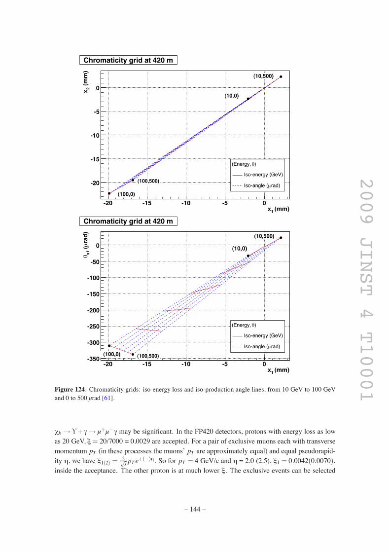
2009 JINST 4 T10001
(mm)1x-20 -15 -10 -5 0
(mm
)2x
-20
-15
-10
-5
0
Chromaticity grid at 420 m
)θ(Energy,
Iso-energy (GeV)
rad)µIso-angle (
(10,0)
(10,500)
(100,0)
(100,500)
(mm)1x-20 -15 -10 -5 0
rad)
µ (x1θ
-350
-300
-250
-200
-150
-100
-50
0
Chromaticity grid at 420 m
)θ(Energy,
Iso-energy (GeV)
rad)µIso-angle (
(10,0)
(10,500)
(100,0) (100,500)
Figure 124. Chromaticity grids: iso-energy loss and iso-production angle lines, from 10 GeV to 100 GeVand 0 to 500 µrad [61].
χb " ϒ+ γ" µ+µ$ γ may be significant. In the FP420 detectors, protons with energy loss as lowas 20 GeV, ξ= 20/7000 = 0.0029 are accepted. For a pair of exclusive muons each with transversemomentum pT (in these processes the muons’ pT are approximately equal) and equal pseudorapid-ity η, we have ξ1(2) = 2)
s pT e+($)η. So for pT = 4 GeV/c and η = 2.0 (2.5), ξ1 = 0.0042(0.0070),
inside the acceptance. The other proton is at much lower ξ. The exclusive events can be selected
– 144 –

2009 JINST 4 T10001
Reconstructed Higgs Mass (GeV)100 110 120 130 140 150
Even
ts
1
10
210
310
with Hector -- "MQXA.1R5" shifted by 0.5mmrecE
MC particles
1.6 GeV)±No misalignment (114.6
1.7 GeV)±Misalignment (108.5
1.6 GeV)±Misalign + beam pos corr. (112.4
1.7 GeV)±Misalign + calibration (114.7
Misalignment impact on Higgs mass reconstruction
Figure 125. Illustration of the effect on the missing mass reconstruction due to a misalignment of LHCquadrupoles. In this example a quadrupole (MQXA1R5) has been misaligned by 500 µm. Data from BPMscannot fully recover the mass shift, while the exclusive dimuon calibration recovers it fully, and the resolutionis not affected as long as the misalignment is stable [61].
in the presence of pile-up, by requiring no other tracks on the dimuon vertex, and Δφµµ . π withpT (µ+) . pT (µ$), or pT (µ+µ$) ! 1 GeV/c, with a coincident consistent track in FP420. Thedominant uncertainty of the forward proton momentum comes from the incoming beam spread(δpp . 10$4 = 700 MeV), as the central dimuons are measured with a better resolution [7]. Thetwo-photon cross section for central “large”-pT muons is small; we expect about 300 events/fb$1
with pT (µ) + 5 GeV/c and |η(µ)| < 2.5. With such good resolution on the predicted proton mo-mentum, combinatorial background can be tolerated and a momentum scale calibration is achievedwith very few (tens of) events, i.e. on a daily basis. However a good measurement of the resolutionwill require more events. A potentially important use of the dimuon events is not only to measurethe spectrometer performance, but to optimise it. For example, different tracking procedures canbe tried and their resolution measured. While the two-photon dimuon events calibrate the missingmass scale in FP420, it cannot be used for frequent re-calibrations of detectors at 220 m as theprocess cross section is much smaller at such high ξ. The ϒ photoproduction is useful not only forimprovement of calibration statistics but also for checking the resolution and bias of the muon pTreconstruction in the central detectors. In addition, the ϒ events can be used to check the forwardproton angular reconstruction.
Other reactions and forward instrumentation can provide information that can be used to cal-ibrate the forward detectors, not as well as exclusive muon pairs but in almost real time. One canmake use for example of the Zero Degree Calorimeter, ZDC, installed at 140 m from both the AT-LAS [103] and CMS [105] IPs. The bremsstrahlung process p+ p" p+ p+ γ with the photons
– 145 –

2009 JINST 4 T10001
emitted into a very forward cone has a cross section of about 10 nb for Eγ > 100 GeV. The photon isdetected in the ZDCs at 140 m, and the proton at 420 m. This allows a cross-calibration; the protonspectrometer is only calibrated as well as the ZDC. The background level (e.g. from forward π2
production) remains to be seen. The angular distribution of bremsstrahlung photons is very forwardpeaked (typically with θ(γ) ! 150 µrad) which helps with background reduction. The flow of neu-tral particles measured at the ZDC is huge and will allow the monitoring of the beam direction (tilt)at the IP with high precision. The LHC luminosity monitors (BRAN) [178] will also be capableof fast online tilt measurement (also bunch-by-bunch) with a resolution better than 10 µrad. Thisinformation together with the precise control of the lateral position of the proton collisions at theIP, provides very good and independent on-line monitoring of the actual proton-beam trajectory.
A measurement of the relative positions of the beam and the track detectors can also comefrom the distributions of single diffractive protons. The less critical vertical (y) distribution peaksat y = ybeam. (This allows a bunch-by-bunch monitor with time of ybeam.) Suppose the horizontalposition to have a poorly known offset δx. Most of the tracks of protons from the intersectionregion will be from single diffraction, p+ p" p+X , which has an exponential t-distribution (atleast in the low |t|-range), dσdt . ebt . The intercept of the distribution at t=0 has a maximum whenthe beam-detector distance is correct, so by applying offsets offline one can find the actual distance.One can also vary the offset to find the maximum slope dσ
dt . This has been successfully applied inCDF [179, 180]; the accuracy on the offset was (at the Tevatron) approximately ±30µm in x and y.
Note that protons with t = 0 (more strictly θ = 0) are inside our acceptance; this is wherethe diffractive cross section has a maximum. An improvement on the method could come from ameasurement of the diffractive mass from the central detector, which would allow this technique tobe used selecting bands of ξ; however that can not be done in the presence of pile-up.17
11.5 Alignment summary
While alignment and calibration issues are crucially important for FP420 tracking, we have viablesolutions to all the issues: within the FP420 arm, over its motion towards the beam, with respectto the passing beam, and through the 420 m spectrometer. We have on-line checks of the protonenergy using bremsstrahlung and displacement from the beam using diffractively scattered protons.Finally, and very important, we will use the p+ p" p+µ+µ$ + p reaction to calibrate, offline,both the mass scale and its resolution, and to optimise the latter. We hope to continue to push themass resolution towards the limit given by the incoming beam momentum spread. It is importantto miminise instabilities (bunch-to-bunch, store-to-store, week-to-week etc.) of LHC elements(especially quadrupole alignments), and to monitor any residual instabilities to allow for off-linecorrections to be applied.
12 Near detector infrastructure and detector services
The tunnel region at the location of the FP420 detectors presents a number of constraints for theinstallation of instrumentation such as FEE, HV and LV power supplies, cooling and detector gas
17One or two bunch crossings with deliberately low luminosity, such that< n>. 1, could be useful for this and manyother reasons.
– 146 –

2009 JINST 4 T10001
Figure 126. Plan view of the tunnel area around FP420 and the available space for equipment and services,as detailed in table 21.
supplies. A plan view of the tunnel area around FP420, showing the available space for servicesand electronics, is shown in figure 126.
Simulations have shown [153] that the zone will be exposed to a reasonably high ra-diation dose. A careful assessment of the possible locations and type of instrumentation istherefore required. Provisionally space has already been reserved underneath adjacent mag-nets upstream and downstream from the NCC where the LV and HV supplies can be placed[yy = L0762023PL, L0762024PL, L0762045PL, L0762046PL, L0722023PL, L0722024PL,L0722045PL, L0722046PL]. Most of the machine electronics is already placed in this volume andsuch reducing the available space. The dose in this position under the arc magnets is expected tobe between 10 and 20 Gy/year. FEE like trigger electronics, alignment and detector positioningcontrol can be installed in cavities of the support beams of the NCC. In order to limit the radiationload on the environment at most to the level estimated with the present configuration, an envelop ofadequate shielding (Pb plates) will be placed around the beam pipes and detectors as described insection 6. It will also be feasible to place some equipment along the LHC tunnel wall underneaththe cable trays which run above the QRL line but the radiation level will be somewhat higher thanunder the dipole magnets.
Currently, active radiation monitoring instrumentation is being installed in the 420m region ofthe LHC tunnel. These monitors will be operational at LHC startup and thus provide valuable datato assess the real radiation levels in the area. At present no general services are provided in the LHCtunnel at the FP420 region. Power- and controls- cables as well as tubes for fibre-optic (FO) willtherefore need to be pulled from the corresponding experimental area to this location. It is thereforeproposed to install additional cable trays next to the overhead rail of the monorail. This strategyhas already been used for the routing of the services for LHCf to both sides of point 1. FP420 canreuse these trays which will have to be extended from the present 150m to 420m. The FP420 powersupplies and detector controls instrumentation could be connected to the LHCmachine power. Thiswould assure the electricity supply as long as the LHC machine power is available and reduce thecabling impact in the tunnel since additional power cables would only need to be routed from the
– 147 –

2009 JINST 4 T10001
Figure 127. Reserved rack space in the LHC alcove areas (RRs).
nearest RR alcoves at a distance of about 200m. Space has also been reserved in the RR13, RR17,RR53, RR57 alcoves on the 2nd floor level above the LHC power converters (figure 127). At thislocation the expected annual fluence of hadrons (E > 20 MeV) is in the order of 108, correspondingto a dose rate in the order of 0.3 Gy per annum, and considered suitable for installation of detectorpower supplies and electronics for the alignment monitoring system.
The assessment of types and quantities of services needed for the FP420 detectors is still ratherdifficult at this stage of the project. Those requirements which correspond to the present estimationfor each sub-system are summarised in table 21.
13 Conclusions
The FP420 project proposes to install silicon trackers and fast timing detectors in the LHC tunnelat 420 m from the interaction points of the ATLAS and CMS experiments for the detection of veryforward protons as a means to study Standard Model (SM) and new physics signals. The FP420detector system is a magnetic spectrometer consisting of a moveable silicon tracking system whichmeasures the spatial position of protons scattered by a few hundreds µrads relative to the LHCbeam, and their arrival times at several points in a 12 m region around 420 m. The measurement ofthe displacement and angle of the outgoing protons relative to the beam allows the reconstruction oftheir momentum loss and transverse momentum. The combined detection of both outgoing protonsand the associated centrally produced system using the current ATLAS and/or CMS detectors givesaccess to a rich programme of studies in QCD, electroweak, Higgs and Beyond the Standard Modelphysics. The addition of such detectors will add the capability to make measurements which arecurrently unique at the LHC, and may be difficult even at a future linear collider.
– 148 –

2009 JINST 4 T10001
Table 21. Summary of detector services required for FP420. Abbreviations: BPM - Beam PositionMonitors,BLM - Beam Loss Monitors, FEE - Front End Electronics, FO - Fibre optics, WPS - Wire PositioningSystem.
Sub-system Requirements Location CommentGasTOF gas Detector station Secondary vacuum
FEE, DAQ Cryostat support beamselec. power see figure 94
Quartic FEE, DAQ Cryostat support beamselec. power see figure 94
3D (Silicon) Cooling Detector stationFEE, DAQ Cryostat support beamselec. power see figure 94
General Cooling power, controlAlignment BPM, BLM, Detector station,
WPS, other Detector support table RRsPositioning Movement drive, Detector support table
control see figure 94Timing TTC, BST Counting roomsInterlocks Injection, Machine IF rack in
Dump exp. counting roomElectrical power 400 V AC RE alcoves UPS for controlled
230 V AC shutdown ?48 V DC
HV 16 ch. HV 4kV see figure 94 Control from IP (CAN bus ?)(timing)36 ch. HV(tracking)
LV 6 ch. LV see figure 94 Control from IP (CAN bus ?)(timing)36 ch. LV(tracking)
Communication, FO, Field bus ECR3" FP420 Space available forRH-diodes: RH-diodes: + 2%24 fibres to each
MITSUBISHI stationFU-427SLD-F1 Use BLM / BPM FEE ?
Miscellaneous Cameras, lights FP420Instrumentation VME crate Cell 12L/R at IP1 & IP5
space equivalent each (5);13.8m tunnel wall;Call 11 L/R (5)
each (5);
A prime process of interest for FP420 is Central Exclusive Production (CEP), pp" p+φ+ p,in which the outgoing protons remain intact and the central system φ may be a single particle suchas a Higgs boson. Observation of new particle production in the CEP channel benefits from (i)
– 149 –

2009 JINST 4 T10001
enhanced signal over backgrounds (giving access to the difficult Higgs fermionic decay channelsfor example), and allows one to directly measure (ii) its quantum numbers (the central systemhas an approximate JPC = 0++ selection rule) as well as (iii) its mass with very good resolution,O(2 GeV/c2) irrespective of the decay channel of the particle. In some beyond-SM scenarios, theFP420 detectors may be the primary means of discovering new particles at the LHC. Section 2of this document has presented an overview of the physics case for FP420 including the currenttheoretical status of CEP predictions. The state-of-the-art calculations of the production crosssection for a 120 GeV/c2 Standard Model Higgs boson via the CEP process at the LHC yields acentral value of 3 fb, with a factor of # 3 uncertainty. Supersymmetric extensions of the SM, yieldHiggs boson cross sections 10 or 100 times larger and would allow the 5σ discovery of all CP-evenscalar bosons in practically the wholeMA$ tanβ plane with O(100 fb$1). Section 3 has presented adetailed study of the trigger strategy, expected acceptance, reconstruction efficiencies, signal overbackgrounds and final mass resolutions and yields for a particular p p" pH p measurement withHiggs boson decay in the bbmode. The Higgs boson line shape in this channel can be reconstructedwith a 3σ or better significance with an integrated luminosity of 60 fb$1.
A summary of various interesting photon-photon and photon-proton processes accessible toFP420 is presented (section 2.8). Photon-induced reactions tagged with forward protons can pro-vide a very clean environment for the study of various signals such as anomalous top or associatedWH production in γ p interactions; as well as anomalous gauge boson couplings, exclusive dilep-tons or supersymmetric pair production in γγ interactions. Hard diffraction studies (single diffrac-tive and double pomeron production of B-mesons,W , Z bosons or di-jets), sensitive to generalisedparton distributions, are discussed in section 2.9.
The beam optics at LHC (section 4) allows protons that have lost momentum in a diffractiveinteraction to emerge from the beam envelope at regions 220 m and 420 m from the interactionpoint. The acceptance of silicon detector arrays in these locations placed at distances 3–9 mm fromthe beam centre allows for the detection of both outgoing protons from centrally produced objectswith a wide range of masses above 60 GeV/c2. However, to obtain good acceptance for massesabove 150 GeV/c2, the 220 m system is essential. The expected position and angle resolutions forthe protons obtained in the silicon stations yield a mass resolution reaching values of 2 to 3 GeV/c2.
The expected machine-induced backgrounds at 420 m such as beam-halo and beam-gas back-grounds are discussed in section 5. Contributions at 420 m from near beam-gas and the betatroncleaning collimation are found to be small. For transverse separations between the detectors and thebeam centre above 5 mm, the integrated number of protons, photons and neutrons from beam halois expected to be less than 1, 0.16 and 0.003 per bunch crossing respectively. The impact of theseestimated background rates needs to be assessed in term of detector performance and survivability.
Section 6 describes the new 420 m connection cryostat which will allow moving near-beamdetectors with no effects on LHC operations. A preliminary design for a replacement connectioncryostat that would allow detectors to be placed in the 420 m region has been completed, and afinal design is in progress. Such a solution is expected to actually lower the dynamic heat loadof the LHC and have similar radiation profiles. With the appropriate approvals and funding, twosuch cryostats could be built and installed in late 2011 (installation time is around 90 days), and inprinciple, two more in 2012 with negligible impact on LHC operations.
The design of the beam pipe in the FP420 region and the movement mechanism are discussed
– 150 –

2009 JINST 4 T10001
in section 7. The Hamburg moving-pipe concept provides the optimal solution for the FP420detector system as it ensures a simple and robust design and good access to the detectors. Moreover,it is compatible with the very limited space available in the modified connection cryostat and withthe expected position of the scattered protons between the two LHC beampipes, and it permits theincorporation of rather large detectors, such as the timing devices, using pockets, i.e. rectangularindentations in the moving pipes. The prototype detector pockets show the desired flatness ofthe thin windows, and the first motorised moving section, with prototype detectors inserted, hasbeen tested at the CERN test beam. A full prototype test, including assembling, positioning andalignment aspects, is planned in test beam in Fall 2009.
The studies of the radio-frequency impact of the design on the LHC are described in section 8.Numerical simulations, analytical calculations and laboratory measurements have showed consis-tently that the proposed FP420 design will have a small impact on the total LHC impedance budget,even for transverse distances of the stations from the beam centre as small as 3 mm. Tapering of thebeam pipe indentations is recommended because it reduces the impedance significantly, as mea-sured both with the single pocket and double pocket designs. The beam harmonics at 2GHz areexpected to be below 10$2 of the main harmonic at 40MHz and well below 10$3 at 2.5 GHz, andthe horizontal tune shift induced by a FP420 station is expected to be almost imperceptible whencompared to the tune stability region defined by the available LHC octupole magnets.
In section 9 we present a detailed description of the design of the FP420 3D silicon sensorsincluding mechanical support system, superlayer and blade design and thermal tests, assembly andalignment, high- and low- voltages, tracker readout, downstream data acquisition and infrastructureat the host experiment. The performance of the tracker has been evaluated using a simple MonteCarlo program as well as a full GEANT4 simulation. Estimates of the multiple scattering for thethree (two) station layouts indicate that the expected angular resolution is 0.85 µrad (0.91 µrad),well within design specifications. The efficiency of two track reconstruction has been found to be86% and 80% respectively for the two and three station layouts.
Since the cross sections for CEP of the SM Higgs boson and other new physics scenariosare relatively small (few fb), FP420 must be designed to operate at the highest LHC instantaneousluminosities of 1034cm$2s$1. A measurement of the relative time of arrival of the two protons atFP420 in the 10 picosecond range is required for matching the detected protons with a central vertexwithin#2mm, which will enable the rejection of a large fraction of the pile-up overlap background.Section 10 describes two complementary fast timing detector designs: GASTOF (GAS Time OfFlight) and QUARTIC (QUARtz TIming Cerenkov). The prototype detector design is approachinga resolution of 20 ps. An upgrade to determine the time of more than one proton per bunch isconceivable, either by reading out individual pixels in the GASTOFMCP-PMT to resolve separate,but overlapping, Cerenkov discs, or by reducing the pixel size in the x-direction for the QUARTICdetectors. We are also developing a promising new type of focusing quartz Cerenkov detector. Asthe reference timing is also an important component of the timing resolution, we are also exploringinterferometrically stabilised fibre optic links, where the standard is in the 10 femtosecond range.
In section 11 we describe the alignment and calibration strategy, using both physics and beamposition monitor techniques. Alignment and calibration is guaranteed for all experimental con-ditions: within the FP420 arm, over its motion towards the beam, with respect to the passingbeam, and through the 420 m spectrometer. We have on-line checks of the proton energy using
– 151 –

2009 JINST 4 T10001
bremsstrahlung and of displacement from the beam using diffractively scattered protons. We willuse the p+ p" p+µ+µ$ + p reaction to calibrate, offline, both the mass scale and its resolution,and to optimise the latter. It is important to miminise instabilities (bunch-to-bunch, store-to-store,week-to-week etc.) of LHC elements (especially quadrupole alignments), and to monitor any resid-ual instabilities to allow for off-line corrections to be applied. Chapter 12 outlines the near detectorinfrastructure and detector services required for the FP420 project.
The studies presented in this document have shown that it is possible to install detectors inthe 420 m region with no impact on the operation or luminosity of the LHC. These detectorscan be aligned and calibrated to the accuracy required to measure the mass of the centrally pro-duced system to between 2 and 3 GeV/c2. This would allow an observation of new particles inthe 60$ 180 GeV/c2 mass range in certain physics scenarios during 3 years of LHC running atinstantaneous luminosities of 2%1033 cm$2 s$1, and in many more scenarios at instantaneous lu-minosities of up to 1034 cm$2 s$1. Events can be triggered using the central detectors alone atLevel 1, using information from the 420 m detectors at higher trigger levels to reduce the eventrate. Observation of new particle production in the CEP channel would allow a direct measurementof the quantum numbers of the particle and an accurate determination of the mass, irrespective ofthe decay channel of the particle. In some scenarios, these detectors may be the primary meansof discovering new particles at the LHC, with unique ability to measure their quantum numbers.The FP420 opens, moreover, the possibility to develop an extensive, high-rate γγ and γp physicsprogram. The addition of the FP420 detectors will thus, for a relatively small cost, significantlyenhance the discovery and physics potential of the ATLAS and CMS experiments.
14 Costing
A preliminary estimate of the costing of the major components of FP420 detectors is given here asan indication. A detailed costing evaluation is still being performed.
• Two new cryostats per experiment, amounting to a total of 1.5 MCHF/experiment
• The silicon tracker including the electronics and mechanical parts: 0.7 to 1.0 MCHF/ exper-iment, depending on the purchasing of equipment
• Quartic timing detectors, including electronics, 100 kCHF/experiment for 4 detectors.
• GASTOF timing detectors, including electronics, DAQ, slow controls and cables: 145 kCHF
• BPMs and beampipe mechanics: 380 kCHF/experiment
• High voltage/Low Voltage: 160 kCHF/experiment
This leads to a approximate grand total of 3.5 MCHF/experiment for equipping both sides withFP420 detectors.
– 152 –

2009 JINST 4 T10001
Acknowledgments
We thank many people in the accelerator (AB and AT) and technical (TS) Departments of CERNfor their valuable help and continuing support in the FP420 design study (beam vacuum, electricalspecifications, RF effects . . . ). In particular, we want to thank Thierry Renaglia, Sebastien Mar-ques, Thierry Colombet, Alain Poncet and Vittorio Parma for their expertise and generous helpwith the cryostat studies. This work was supported in the UK by grants from the STFC and theRoyal Society; in the USA by the Department of Energy (including Fermilab and Brookhaven Na-tional Lab funding, UT-Arlington base funding and the Advanced Detector Research program),and the Texas Advanced Research Program; in Belgium by FNRS and its associated fund (IISN),by FWO-Vlaanderen, IIKW, and by the Inter-University Attraction Poles Programme subsidisedby the Belgian Federal Science Policy; in Italy by the Italian Istituto Nazionale di Fisica Nucleare(INFN) and by the Italian Ministry for Education, University and Scientific Research under theprogramme “Incentivazione alla mobilita di studiosi stranieri e italiani residenti all’estero”.
References
[1] M.G. Albrow and A. Rostovtsev, Searching for the Higgs at hadron colliders using the missing massmethod, hep-ph/0009336.
[2] V.A. Khoze, A.D. Martin and M.G. Ryskin, Prospects for new physics observations in diffractiveprocesses at the LHC and Tevatron, Eur. Phys. J. C 23 (2002) 311 [hep-ph/0111078].
[3] B.E. Cox, A review of forward proton tagging at 420 m at the LHC and relevant results from theTevatron and HERA, AIP Conf. Proc. 753 (2005) 103 [hep-ph/0409144].
[4] V.A. Khoze, A.B. Kaidalov, A.D. Martin, M.G. Ryskin and W.J. Stirling, Diffractive processes as atool for searching for new physics, in the proceedings of Gribov-75 Memorial Workshop, Budapest,2005 hep-ph/0507040.
[5] J.R. Forshaw, Diffractive Higgs production: theory, contributed to HERA and the LHC: A Workshopon the Implications of HERA and LHC Physics, hep-ph/0508274.
[6] K. Piotrzkowski, Tagging two-photon production at the LHC, Phys. Rev. D 63 (2001) 071502[hep-ex/0009065].
[7] [FP-420] M. Albrow et al., FP420: An R&D Proposal to Investigate the Feasibility of InstallingProton Tagging Detectors in the 420 m Region of the LHC, CERN-LHCC-2005-025, LHCC-I-015.
[8] CMS AND TOTEM collaborations, M. Albrow et al., Prospects for diffractive and forward physicsat the LHC, CERN-LHCC-2006-039.
[9] S. Ask, Status of the Forward Physics Projects in ATLAS, arXiv:0706.0644.
[10] RP220 collaboration, C. Royon, Project to install roman pot detectors at 220 m in ATLAS,arXiv:0706.1796.
[11] P.J. Bussey, T.D. Coughlin, J.R. Forshaw and A.D. Pilkington, Central exclusive production of longlived gluinos at the LHC, JHEP 11 (2006) 027 [hep-ph/0607264].
[12] J. Favereau de Jeneret et al., High energy photon interactions at the LHC, CP3-08-04 (June 2008),arXiv:0908.2020.
– 153 –

2009 JINST 4 T10001
[13] V.A. Khoze, A.D. Martin and M.G. Ryskin, Double diffractive processes in high resolution missingmass experiments at the Tevatron, Eur. Phys. J. C 19 (2001) 477 [hep-ph/0011393].
[14] A. De Roeck, V.A. Khoze, A.D. Martin, R. Orava and M.G. Ryskin,Ways to detect a light Higgsboson at the LHC, Eur. Phys. J. C 25 (2002) 391 [hep-ph/0207042].
[15] A.B. Kaidalov, V.A. Khoze, A.D. Martin and M.G. Ryskin, Extending the study of the Higgs sector atthe LHC by proton tagging, Eur. Phys. J. C 33 (2004) 261 [hep-ph/0311023].
[16] B.E. Cox et al., Detecting the standard model Higgs boson in the W W decay channel using forwardproton tagging at the LHC, Eur. Phys. J. C 45 (2006) 401 [hep-ph/0505240].
[17] V.A. Khoze, M.G. Ryskin and W.J. Stirling, On radiative QCD backgrounds to exclusive H" banti-b production at the LHC and a photon collider, Eur. Phys. J. C 48 (2006) 477[hep-ph/0607134].
[18] V.A. Khoze, A.D. Martin and M.G. Ryskin, Insight into double pomeron exchange Higgs productionand backgrounds, Phys. Lett. B 650 (2007) 41 [hep-ph/0702213].
[19] S. Heinemeyer et al., Studying the MSSM Higgs sector by forward proton tagging at the LHC,Eur. Phys. J. C 53 (2008) 231 [arXiv:0708.3052];S. Heinemeyer, V.A. Khoze, M.G. Ryskin, M. Tasevsky and G. Weiglein, Central ExclusiveProduction of BSM Higgs bosons at the LHC, arXiv:0811.4571.
[20] B.E. Cox, F.K. Loebinger and A.D. Pilkington,Detecting Higgs bosons in the bb decay channel usingforward proton tagging at the LHC, JHEP 10 (2007) 090 [arXiv:0709.3035].
[21] V.A. Khoze, A.D. Martin and M.G. Ryskin, Photon exchange processes at hadron colliders as aprobe of the dynamics of diffraction, Eur. Phys. J. C 24 (2002) 459 [hep-ph/0201301].
[22] M.G. Ryskin, A.D. Martin and V.A. Khoze, Soft diffraction at the LHC: a partonic interpretation,Eur. Phys. J. C 54 (2008) 199 [arXiv:0710.2494];A.D. Martin, V.A. Khoze and M.G. Ryskin, Rapidity gap survival probability and total crosssections, arXiv:0810.3560.
[23] V.A. Khoze, A.D. Martin and M.G. Ryskin, Soft diffraction and the elastic slope at Tevatron andLHC energies: a multi-pomeron approach, Eur. Phys. J. C 18 (2000) 167 [hep-ph/0007359].
[24] E. Gotsman, E. Levin and U. Maor, A Soft Interaction Model at Ultra High Energies: amplitudes,Cross Sections and Survival Probabilities, arXiv:0708.1506.
[25] G. Weiglein, SUSY Higgs bosons at the LHC, arXiv:0709.4408.
[26] J.R. Ellis, J.S. Lee and A. Pilaftsis, Diffraction as a CP and lineshape analyzer for MSSM Higgsbosons at the LHC, Phys. Rev. D 71 (2005) 075007 [hep-ph/0502251].
[27] J.R. Forshaw, J.F. Gunion, L. Hodgkinson, A. Papaefstathiou and A.D. Pilkington, Reinstating the’no-lose’ theorem for NMSSM Higgs discovery at the LHC, JHEP 04 (2008) 090[arXiv:0712.3510].
[28] V.A. Khoze, A.D. Martin and M.G. Ryskin, Hunting a light CP-violating Higgs via diffraction at theLHC, Eur. Phys. J. C 34 (2004) 327 [hep-ph/0401078].
[29] V.A. Khoze, A.D. Martin and M.G. Ryskin, Can the Higgs be seen in rapidity gap events at theTevatron or the LHC?, Eur. Phys. J. C 14 (2000) 525 [hep-ph/0002072].
[30] V.A. Khoze, A.D. Martin and M.G. Ryskin, Physics with tagged forward protons at the LHC,Eur. Phys. J. C 24 (2002) 581 [hep-ph/0203122].
– 154 –

2009 JINST 4 T10001
[31] X.-D. Ji, Deeply-virtual Compton scattering, Phys. Rev. D 55 (1997) 7114 [hep-ph/9609381].
[32] A.V. Radyushkin, Asymmetric gluon distributions and hard diffractive electroproduction,Phys. Lett. B 385 (1996) 333 [hep-ph/9605431].
[33] J.D. Bjorken, Rapidity gaps and jets as a new physics signature in very high-energy hadron hadroncollisions, Phys. Rev. D 47 (1993) 101.
[34] S. Alekhin, E. Gotsman, E. Levin, U. Maor, E. Naftali and A. Prygarin, Survival probability of largerapidity gaps, in HERA and the LHC - A workshop on the implications of HERA for LHC physics:proceedings Part A, hep-ph/0601012.
[35] L. Frankfurt, C.E. Hyde, M. Strikman and C. Weiss, Generalized parton distributions and rapiditygap survival in exclusive diffractive pp scattering, Phys. Rev. D 75 (2007) 054009[hep-ph/0608271].
[36] V.A. Khoze, A.D. Martin and M.G. Ryskin, Early LHC measurements to check predictions forcentral exclusive production, Eur. Phys. J. C 55 (2008) 363 [arXiv:0802.0177].
[37] CDF collaboration, T. Aaltonen et al., Observation of Exclusive Dijet Production at the FermilabTevatron p$ p Collider, Phys. Rev. D 77 (2008) 052004 [arXiv:0712.0604].
[38] CDF collaboration, T. Aaltonen et al., Search for exclusive γγ production in hadron- hadroncollisions, Phys. Rev. Lett. 99 (2007) 242002 [arXiv:0707.2374].
[39] CDF collaboration, T. Aaltonen et al., Observation of exclusive charmonium production andgamma+gamma to µ+µ$ in p+pbar collisions at sqrts = 1.96 TeV,Phys. Rev. Lett. 102 (2009) 242001 [arXiv:0902.1271].
[40] A. Vilela Pereira, A study of central exclusive production of H"WW at CMS, FP420 Note2008-002, http://www.fp420.com.
[41] M.S. Carena, S. Heinemeyer, C.E.M. Wagner and G. Weiglein, Suggestions for benchmark scenariosfor MSSM Higgs boson searches at hadron colliders, Eur. Phys. J. C 26 (2003) 601[hep-ph/0202167].
[42] LEP WORKING GROUP FOR HIGGS BOSON SEARCHES collaboration, R. Barate et al., Search forthe standard model Higgs boson at LEP, Phys. Lett. B 565 (2003) 61 [hep-ex/0306033].
[43] ALEPH collaboration, S. Schael et al., Search for neutral MSSM Higgs bosons at LEP,Eur. Phys. J. C 47 (2006) 547 [hep-ex/0602042].
[44] J.R. Ellis, J.F. Gunion, H.E. Haber, L. Roszkowski and F. Zwirner, Higgs Bosons in a NonminimalSupersymmetric Model, Phys. Rev. D 39 (1989) 844.
[45] R. Dermisek and J.F. Gunion, Escaping the large fine tuning and little hierarchy problems in the nextto minimal supersymmetric model and h" a a decays, Phys. Rev. Lett. 95 (2005) 041801[hep-ph/0502105].
[46] U. Ellwanger, J.F. Gunion and C. Hugonie,Difficult scenarios for NMSSM Higgs discovery at theLHC, JHEP 07 (2005) 041 [hep-ph/0503203].
[47] K. Belotsky, V.A. Khoze, A.D. Martin and M.G. Ryskin, Can an invisible Higgs boson be seen viadiffraction at the LHC?, Eur. Phys. J. C 36 (2004) 503 [hep-ph/0406037].
[48] CDF collaboration, A. Abulencia et al., Observation of exclusive electron positron production inhadron hadron collisions, Phys. Rev. Lett. 98 (2007) 112001 [hep-ex/0611040].
– 155 –

2009 JINST 4 T10001
[49] CDF collaboration, T. Aaltonen et al., Search for exclusive Z boson production and observation ofhigh mass pp" p+ γγ+ p" p+ !!+ p events in pp collisions at
)s = 1.96 TeV,
Phys. Rev. Lett. 102 (2009) 222002 [arXiv:0902.2816].
[50] PHENIX collaboration, D.G. d’Enterria, Coherent photoproduction of J/psi and high-mass e+e$pairs in ultra-peripheral Au + Au collisions at)sNN = 200GeV , nucl-ex/0601001.
[51] V.M. Budnev, I.F. Ginzburg, G.V. Meledin and V.G. Serbo, The two photon particle productionmechanism. Physical problems. Applications. Equivalent photon approximation,Phys. Rept. 15 (1974) 181.
[52] K. Hencken et al., The physics of ultraperipheral collisions at the LHC, Phys. Rept. 458 (2008) 1[arXiv:0706.3356].
[53] F. Maltoni and T. Stelzer,MadEvent: automatic event generation with MadGraph,JHEP 02 (2003) 027 [hep-ph/0208156];T. Stelzer and W.F. Long, Automatic generation of tree level helicity amplitudes,Comput. Phys. Commun. 81 (1994) 357.
[54] A. Pukhov, Adaptation of Vegas for event generation, Nucl. Instrum. Meth. A 502 (2003) 596.
[55] S.P. Baranov et al., LPAIR: A generator for lepton pair production, in Proceedings of Physics atHERA Workshop (1991), pg. 1478.
[56] T. Sjostrand et al., High-energy physics event generation with PYTHIA 6.1,Comput. Phys. Commun. 135 (2001) 238 [hep-ph/0010017].
[57] J. Ohnemus, T.F. Walsh and P.M. Zerwas, Gamma gamma production of nonstrongly interactingSUSY particles at hadron colliders, Phys. Lett. B 328 (1994) 369 [hep-ph/9402302].
[58] J.F. Gunion and H.E. Haber, Higgs boson production in the photon-photon collider mode of ahigh-energy e+e$ linear collider, Phys. Rev. D 48 (1993) 5109.
[59] V.M. Budnev, I.F. Ginzburg, G.V. Meledin and V.G. Serbo, The process p p" p p e+e$ and thepossibility of its calculation by means of quantum electrodynamics only, Nucl. Phys. B 63 (1973) 519;A.G. Shamov and V.I. Telnov, Precision luminosity measurement at LHC using two-photonproduction of µ+µ$ pairs, Nucl. Instrum. Meth. A 494 (2002) 51 [hep-ex/0207095];D. Bocian and K. Piotrzkowski, Very forward two-photon e+e- production and luminositymeasurements for ion collisions at the LHC, Acta Phys. Polon. B 35 (2004) 2417;M.W. Krasny, J. Chwastowski and K. Slowikowski, Luminosity measurement method for LHC: thetheoretical precision and the experimental challenges, Nucl. Instrum. Meth. A 584 (2008) 42[hep-ex/0610052];J.A.M. Vermaseren, Two Photon Processes at Very High-Energies, Nucl. Phys. B 229 (1983) 347.
[60] V.A. Khoze, A.D. Martin, R. Orava and M.G. Ryskin, Luminosity monitors at the LHC,Eur. Phys. J. C 19 (2001) 313 [hep-ph/0010163].
[61] J. de Favereau, X. Rouby and K. Piotrzkowski, Hector, a fast simulator for the transport of particlesin beamlines, 2007 JINST 2 P09005 [arXiv:0707.1198].
[62] G. Belanger and F. Boudjema, Probing quartic couplings of weak bosons through three vectorsproduction at a 500-GeV NLC, Phys. Lett. B 288 (1992) 201.
[63] OPAL collaboration, G. Abbiendi et al., Constraints on anomalous quartic gauge boson couplingsfrom nu anti-nu gamma gamma and q anti-q gamma gamma events at LEP2,Phys. Rev. D 70 (2004) 032005 [hep-ex/0402021].
– 156 –

2009 JINST 4 T10001
[64] O. Kepka and C. Royon, Anomalous WWgamma coupling in photon-induced processes using forwarddetectors at the LHC, Phys. Rev. D 78 (2008) 073005 [arXiv:0808.0322].
[65] G. Bhattacharya, P. Kalyniak and K.A. Peterson, Photon and Z induced heavy charged lepton pairproduction at a hadron supercollider, Phys. Rev. D 53 (1996) 2371 [hep-ph/9512255].
[66] M. Drees, R.M. Godbole, M. Nowakowski and S.D. Rindani, gamma gamma processes athigh-energy p p colliders, Phys. Rev. D 50 (1994) 2335 [hep-ph/9403368].
[67] G. Bhattacharya, P.A. Kalyniak and K.A. Peterson, Heavy charged lepton pair production throughphoton fusion at hadron supercolliders, hep-ph/9310223.
[68] DELPHI collaboration, J. Abdallah et al., Searches for supersymmetric particles in e+e$ collisionsup to 208-GeV and interpretation of the results within the MSSM, Eur. Phys. J. C 31 (2003) 421[hep-ex/0311019].
[69] OPAL collaboration, G. Abbiendi et al., Search for anomalous production of di-lepton events withmissing transverse momentum in e+e$ collisions at
)s= 183GeV–209GeV,
Eur. Phys. J. C 32 (2004) 453 [hep-ex/0309014].
[70] M. Battaglia et al., Updated post-WMAP benchmarks for supersymmetry,Eur. Phys. J. C 33 (2004) 273 [hep-ph/0306219].
[71] K.-m. Cheung, Photoproduction of W H signal at electron-proton colliders,Phys. Lett. B 319 (1993) 244 [hep-ph/9401316].
[72] T. Han and J.L. Hewett, Top charm associated production in high-energy e+e$ collisions,Phys. Rev. D 60 (1999) 074015 [hep-ph/9811237].
[73] ZEUS collaboration, S. Chekanov et al., Search for single-top production in e p collisions at HERA,Phys. Lett. B 559 (2003) 153 [hep-ex/0302010].
[74] J. Hollar, S. Ovyn and X. Rouby, Exclusive γγ" !+!$ and γp" ϒp" !+!$p production,CMS-PAS-DIF-07-001, CMS-AN-2007-032.
[75] I. I. Balitsky and L. N. Lipatov, The Pomeranchuk singularity, process, theory, Sov. J. Nucl. Phys. 28(1978) 822 [Yad. Fiz. 28 (1978) 1597];E.A. Kuraev, L.N. Lipatov and V.S. Fadin,Multi - Reggeon Processes in the Yang-Mills Theory, Sov.Phys. JETP 44 (1976) 443.
[76] UA8 collaboration, A. Brandt et al., Evidence for a superhard pomeron structure,Phys. Lett. B 297 (1992) 417.
[77] V. Barone and E. Predazzi, High-energy particle diffraction, Springer (2002).
[78] S. Alekhin et al., HERA and the LHC - A workshop on the implications of HERA for LHC physics:proceedings Part B, hep-ph/0601013.
[79] M. Arneodo and M. Diehl, Diffraction for non-believers, hep-ph/0511047.
[80] ZEUS collaboration, S. Chekanov et al., Leading proton production in e+ p collisions at HERA,Nucl. Phys. B 658 (2003) 3 [hep-ex/0210029].
[81] A.B. Kaidalov et al., Probabilities of rapidity gaps in high-energy interactions, Eur. Phys. J. C 21(2001) 521 [hep-ph/0105145].
[82] B.E. Cox and J.R. Forshaw, POMWIG: HERWIG for diffractive interactions,Comput. Phys. Commun. 144 (2002) 104 [hep-ph/0010303].
– 157 –

2009 JINST 4 T10001
[83] CMS collaboration, G.L. Bayatian et al., CMS technical design report, volume II: physicsperformance, J. Phys. G 34 (2007) 995.
[84] OSCAR: CMS Simulation Package, http://cmsdoc.cern.ch/oscar.
[85] ORCA: CMS Reconstruction Package, http://cmsdoc.cern.ch/orca.
[86] V.A. Khoze, A.D. Martin and M.G. Ryskin, The extraction of the bare triple-pomeron vertex: acrucial ingredient for diffraction, Phys. Lett. B 643 (2006) 93 [hep-ph/0609312].
[87] M. Boonekamp and T. Kucs, POMWIG v2.0: updates for double diffraction,Comput. Phys. Commun. 167 (2005) 217 [hep-ph/0312273].
[88] CMS collaboration, D. Acosta et al., CMS Physics TDR Volume 1, Section 2.6: Fast simulation,CERN-LHCC-2006-001 (2006), p. 55.
[89] H1 collaboration, C. Adloff et al., Inclusive measurement of diffractive deep inelastic ep scattering,Z. Phys. C 76 (1997) 613 [hep-ex/9708016].
[90] E. Accomando et al.,Workshop on CP Studies and Non-Standard Higgs Physics, hep-ph/0608079.
[91] M.S. Carena, J.R. Ellis, A. Pilaftsis and C.E.M. Wagner, CP-violating MSSM Higgs bosons in thelight of LEP 2, Phys. Lett. B 495 (2000) 155 [hep-ph/0009212]; Renormalization-group-improvedeffective potential for the MSSM Higgs sector with explicit CP-violation, Nucl. Phys. B 586 (2000) 92[hep-ph/0003180].
[92] J.M. Maldacena, The large-N limit of superconformal field theories and supergravity, Adv. Theor.Math. Phys. 2 (1998) 231 [Int. J. Theor. Phys. 38 (1998) 1113] [hep-th/9711200];E. Witten, Anti-de Sitter space, thermal phase transition and confinement in gauge theories, Adv.Theor. Math. Phys. 2 (1998) 505 [hep-th/9803131].
[93] H. Liu, Heavy ion collisions and AdS/CFT, J. Phys.G 34 (2007) S361 [hep-ph/0702210].
[94] R.C. Brower, M.J. Strassler and C.-I. Tan, On the pomeron at Large ’t Hooft Coupling,JHEP 03 (2009) 092 [arXiv:0710.4378].
[95] A.R. White, The Physics of a sextet quark sector, Phys. Rev. D 72 (2005) 036007 [hep-ph/0412062].
[96] A.R. White, Unification of the standard model via high-energy unitarity, hep-ph/0611262 andreferences therein.
[97] J. Monk and A. Pilkington, ExHuME: a Monte Carlo event generator for exclusive diffraction,Comput. Phys. Commun. 175 (2006) 232 [hep-ph/0502077].
[98] V.A. Khoze, M.G. Ryskin and W.J. Stirling, On radiative QCD backgrounds to exclusive H" banti-b production at the LHC and a photon collider, Eur. Phys. J. C 48 (2006) 477[hep-ph/0607134].
[99] H1 collaboration, A. Aktas et al.,Measurement and QCD analysis of the diffractive deep- inelasticscattering cross-section at HERA, Eur. Phys. J. C 48 (2006) 715 [hep-ex/0606004].
[100] V.A. Khoze, A.D. Martin and M.G. Ryskin, Insight into double-pomeron-exchangeHiggs productionand backgrounds, Phys. Lett. B 650 (2007) 41 [hep-ph/0702213].
[101] G. Corcella et al., HERWIG 6.5: an event generator for Hadron Emission Reactions With InterferingGluons (including supersymmetric processes), JHEP 01 (2001) 010 [hep-ph/0011363].
[102] J.M. Butterworth, J.R. Forshaw and M.H. Seymour,Multiparton interactions in photoproduction atHERA, Z. Phys. C 72 (1996) 637 [hep-ph/9601371].
[103] ATLAS collaboration, S.N. White et al., Zero Degree Calorimeters for ATLAS,CERN-LHCC-2007-001.
– 158 –

2009 JINST 4 T10001
[104] X. Aslanoglou et al., Performance Studies of Prototype-II for the CASTOR forward Calorimeter atthe CMS Experiment, Eur. Phys. J. C 52 (2007) 495 [arXiv:0706.2641].
[105] CMS collaboration, O.A. Grachov et al., Status of zero degree calorimeter for CMS experiment,AIP Conf. Proc. 867 (2006) 258 [nucl-ex/0608052].
[106] V.A. Khoze, A.D. Martin and M.G. Ryskin, Central jet production as a probe of the perturbativeformalism for exclusive diffraction, Eur. Phys. J. C 48 (2006) 467 [hep-ph/0605113].
[107] CDF RUN II collaboration, R. Field, CDF run II Monte-Carlo tunes, FERMILAB-PUB-06-408-E.
[108] T. Sjostrand, L. Lonnblad and S. Mrenna, PYTHIA 6.2: physics and manual, hep-ph/0108264.
[109] A. Shuvaev, V.A. Khoze, A.D. Martin and M.G. Ryskin, One-loop gg" b effects in the mainirreducible background to exclusive H " bb production at the LHC, Eur. Phys. J. C 56 (2008) 467[arXiv:0806.1447].
[110] R. Engel and J. Ranft, Hadronic photon-photon interactions at high-energies,Phys. Rev. D 54 (1996) 4244 [hep-ph/9509373].
[111] P.J. Bussey and W. Plano, FPTrack, in preparation.
[112] I. Agapov, J. Carter, G.A. Blair and O. Dadoun, BDSIM: Beamline simulation toolkit based onGEANT4, EuroTeV Report 2006-035.
[113] I. Azhgirey and V. Talanov, The status of MARS program complex, in Proceedings of XVIIIWorkshop on the charged particles accelerators, Vol. 2, pg. 184, Protvino (2000).
[114] Minutes of the CERN Machine Induced Background Working Group, 14-Dec-2007,http://indico.cern.ch/conferenceDisplay.py?confId=24799.
[115] A. Rossi, Residual Gas Density Estimations in the LHC Insertion Regions IR1 and IR5 and theExperimental Regions of ATLAS and CMS for Different Beam Operations,CERN-LHC-Project-Report-783 (2004).
[116] O. Bruning et al., Vacuum System, LHC Design Report, Vol. 1, Chapter 12, CERN-2004-003, CERN,Geneva, Switzerland (2004).
[117] O. Bruning et al., Beam Cleaning and Collimation System, LHC Design Report, Vol. 1, Chapter 18,CERN-2004-003, CERN, Geneva, Switzerland (2004).
[118] LHC collimation homepage, http://lhc-collimation-project.web.cern.ch/.
[119] G. Robert-Demolaize, Design and Performance Optimization of the LHC Collimation System,LHC-Project-Note-981, CERN, Geneva Switzerland (2006).
[120] I. Baishev, Proton Losses in the LHC due to Momentum Cleaning at Top Energy,CERN-LHC-Project-note-407 (2007).
[121] GEANT4 collaboration, S. Agostinelli et al., GEANT4: a simulation toolkit,Nucl. Instrum. Meth. A 506 (2003) 250.
[122] S. Roesler, R. Engel and J. Ranft, The Monte Carlo event generator DPMJET-III, hep-ph/0012252.
[123] MADX homepage, http://mad.web.cern.ch/mad/.
[124] O. Bruning et al., LHC Design Report Vol. 1, CERN-2004-003, CERN, Geneva Switzerland (2004).
[125] T. Columbet, Cryogenics preliminary calculation for the FP420 cryostat,https://edms.cern.ch/document/827775.
[126] S. Pattalwar et al., A New Connection Cryostat to insert FP420 Proton Tagging Detectors in theLHC Ring, Proc. APAC (2007) 103.
– 159 –

2009 JINST 4 T10001
[127] R. Folch, FP420 Cryostat Modules Workpackage, https://edms.cern.ch/document/823322.
[128] K. Piotrzkowski and U. Schneekloth, Photoproduction tagger at 44 m, ZEUS collaboration meeting,March 1994, DESY, Hamburg.
[129] ZEUS collaboration, S. Chekanov et al.,Measurement of proton dissociative diffractivephotoproduction of vector mesons at large momentum transfer at HERA,Eur. Phys. J. C 26 (2003) 389 [hep-ex/0205081];ZEUS collaboration, J. Breitweg et al., Measurement of Dijet photoproduction at high transverseenergies at HERA, Eur. Phys. J. C 11 (1999) 35 [hep-ex/9905046];H1 collaboration, A. Aktas et al., Diffractive photoproduction of ρ mesons with large momentumtransfer at HERA, Phys. Lett. B 638 (2006) 422.
[130] Centre de Recherche du Cyclotron (CRC), UC Louvain, http://www.cyc.ucl.ac.be/.
[131] TOTEM collaboration, V. Berardi et al., TOTEM TDR, CERN-LHC-2004-002, Jan 2004.
[132] A. Mapelli et al., Development of a detector (ALFA) to measure the absolute LHC luminosity atATLAS, in 10th ICATPP Conference, ATL-COM-LUM-2007-008, ATL-LUM-PUB-2007-006.
[133] O. Aberle et al., The Mechanical Design for the LHC Collimators, EPAC-2004-MOPLT008, Jul.2004;R. Losito and A. Masi, LHC Collimators low level control system,IEEE Trans. Nucl. Sci. 55 (2008) 33, RT2007-CM-EXIST04, April 2007;R.W. Assmann et al., The LHC Collimator Controls Architecture Design and Beam Tests,PAC07-MOPAN081, Jun 2007.
[134] A. Guerrero et al., CERN front-end software architecture for accelerator controls, in Gyeongju 2003,Accelerator and large experimental physics control systems, ICALEPCS 2003, Korea, Oct 2003, pg.342.
[135] D. Brandt and L. Vos, Resistive wall instability for the LHC: intermediate review,LHC-PROJECT-NOTE-257, CERN, Geneva, Switzerland (2001).
[136] D. Brandt and L. Vos, Resistive Wall PAC, CERN.
[137] F. Caspers, Impedance determination, Handbook of Accelerator Physics and Engineering, WorldScientific (1999).
[138] V.G. Vaccaro, Coupling Impedance Measurements, INFN-TC-94-023 (1994).
[139] Ansoft Corporation, http://www.ansoft.com/.
[140] Computer Simulation Technology, http://www.cst.com/.
[141] GdfidL Electromagnetic Field simulator, http://www.gdfidl.de/.
[142] F. Roncarolo, R. Appleby and R.M. Jones, Beam Coupling Impedance Simulations andMeasurements for the LHC FP420 Detector, in Proceedings of 22nd Particle Accelerator Conference,Albuquerque, NM (2007).
[143] E. Metral, Overview of Impedance and Single-Beam Instability Mechanisms, CERN-AB-2005-041.
[144] S.I. Parker, C.J. Kenney and J. Segal, 3-D: a New architecture for solid state radiation detectors,Nucl. Instrum. Meth. A 395 (1997) 328.
[145] C. Kenney, S. Parker, J. Segal and C. Storment, Comparison of 3D and planar silicon detectors,Proceedings 9th Meeting of the Division of Particles and Fields of the APS Vol. 2, Minneapolis, MN,11-15 Aug 1996, World Scientific (1998) pg. 1342.
– 160 –
2009 JINST 4 T10001
[146] C. Kenney, S. Parker, J. Segal and C. Storment, Silicon detectors with 3-D electrode arrays:fabrication and initial test results, IEEE Trans. Nucl. Sci. 46 (1999) 1224.
[147] C.J. Kenney et al., Observation of Beta and x-rays with 3D-Architecture, Silicon Micro-StripSensors, IEEE Trans. Nucl. Sci. 48 (2001) 189.
[148] S.I. Parker and C.J. Kenney, Performance of 3$D architecture silicon sensors after intense protonirradiation, IEEE Trans. Nucl. Sci. 48 (2001) 1629.
[149] C.J. Kenney, S.I. Parker and E. Walckiers, Results from 3D sensors with wall electrodes:near-cell-edge sensitivity measurements as a preview of active-edge sensors,IEEE Trans. Nucl. Sci. 48 (2001) 2405.
[150] C. Da Via, Radiation hard silicon detectors lead the way, CERN Courier 43 (2003) 223.
[151] C. Da Via et al., Advances in silicon detectors for particle tracking in extreme radiationenvironments, Nucl. Instrum. Meth. A 509 (2003) 86.
[152] J. Morse et al., The spatial and energy response of a 3d architecture silicon detector measured with asynchrotron x-ray microbeam, Nucl. Instrum. Meth. A 524 (2004) 236.
[153] C.J. Kenney et al., Active-edge planar radiation sensors, Nucl. Instrum. Meth. A 565 (2006) 272.
[154] S.I. Parker et al., 3DX: An X-ray pixel array detector with active edges,IEEE Trans. Nucl. Sci. 53 (2006) 1676.
[155] C. Da Via et al., Radiation hardness properties of 3D active edge silicon detectors,Nucl. Instrum. Meth. 587 (2008) 243.
[156] C. Da Via et al., 3D Active edge silicon detector tests with 120 GeV muons,IEEE Trans. Nucl. Sci. 56 (2009) 505.
[157] C. DaVia, S. Parker and G. Darbo, Development, Testing and Industrialization of Full-3DActive-Edge and Modified-3D Silicon Radiation Pixel Sensors, ATL-P-MN-0022,https://edms.cern.ch/document/828969/1
[158] H.E. Larsen, High voltage bias and low voltage power supply, FP420-Note-2008-001,http://www.fp420.com.
[159] T. Wijnands (CERN-TS), private communication (2007).
[160] ATLAS collaboration, ATLAS: Detector and physics performance technical design report Vol. 1,CERN-LHCC-99-014, ATLAS-TDR-014 (1999); ATLAS: Detector and physics performancetechnical design report Vol. 2, CERN-LHCC-99-015, ATLAS-TDR-015 (1999).
[161] Picosecond Timing Workshop, University of Chicago, March 2008,http://www.hep.anl.gov/ertley/tof/;Argonne National Laboratory, February 2009, http://www.hep.anl.gov/byrum/tof/.
[162] A.N. Akindinov et al., Design aspects and prototype test of a very precise TDC system implementedfor the multigap RPC of the ALICE-TOF, Nucl. Instrum. Meth. A 533 (2004) 178.
[163] M. Akatsu et al.,MCP-PMT timing property for single photons,Nucl. Instrum. Meth. A 528 (2004) 763;K. Inami, N. Kishimoto, Y. Enari, M. Nagamine and T. Ohshima, A 5-ps TOF-counter with anMCP-PMT, Nucl. Instrum. Meth. A 560 (2006) 303.
[164] http://www.hamamatsu.com.
[165] http://www.photek.co.uk.
– 161 –

2009 JINST 4 T10001
[166] Burle http://www.burle.com and Photonis http://www.photonis.commerged in 2005.
[167] N. Kishimoto, M. Nagamine, K. Inami, Y. Enari and T. Ohshima, Lifetime of MCP-PMT,Nucl. Instrum. Meth. A 564 (2006) 204.
[168] S.N. White, On the Correlation of Subevents in the ATLAS and CMS/Totem Experiments,arXiv:0707.1500.
[169] C. Bovet et al., LHC BPM design, CERN-SL-97-069-BI.
[170] E. Calvo et al., The LHC Orbit and Trajectory System, proceedings of DIPAC 2003Mainz, Germany,p. 187.
[171] H. Grote et al., Contributions of the SL Division to the Workshop on Beam-beam Effects at Fermilab,June 2001, CERN-LHC-Project-Report-502.
[172] M. Slater et al., Cavity BPM tests for the ILC energy spectrometer, SLAC-PUB-13031.
[173] S. Walston et al., Performance of a High Resolution Cavity Beam Position Monitor System,Nucl. Instrum. Meth. A 578 (2007) 1.
[174] W. Coosemans et al., Accuracy of the LEP Spectrometer Beam Orbit Monitors,CERN-SL-2001-022-BI.
[175] http://meas-spec.com/myMeas/MEAS download/ApplicationNotes/Position/SchaevitzCernWP 0507.pdf.
[176] F.C. Iselin, J.M. Jowett, J. Pancin and A. Adelmann,MAD Version 9, CERN-SL-2000-026-AP
[177] CDF collaboration, A. Abulencia et al., Observation of exclusive electron positron production inhadron hadron collisions, Phys. Rev. Lett. 98 (2007) 112001 [hep-ex/0611040].
[178] J. Poole ed., Beam Instrumentation, CERN-Report-2004-05-13,https://edms.cern.ch/file/445861/6/Vol 1 Chapter 13.pdf
[179] M. Gallinaro and K. Goulianos,Measurement of the t-distribution in diffractive events using theCDF Roman pot detector, CDF-Internal-note-7877 (2006).
[180] CDF collaboration, M. Gallinaro, Diffractive and exclusive measurements at CDF,hep-ex/0606024.
– 162 –