the fiscal treatment of company cars in belgium · working paper 3-16 the fiscal treatment of...

WORKING PAPER 3-16

The fiscal treatment of company cars in Belgium:

Effects on car demand, travel behaviour and external costs February 2016

Benoit Laine, [email protected],

Alex Van Steenbergen, [email protected]

Federal Planning Bureau Econ omi c an alyses and foreca st s

Avenue des Arts 47-49 – Kunstlaan 47-49

1000 Brussels

E-mail: [email protected]

http://www.plan.be

mailto:[email protected]


http://www.plan.be/

Federal Planning Bureau

The Federal Planning Bureau (FPB) is a public agency.

The FPB performs research on economic, social-economic and environmental policy issues. For that

purpose, the FPB gathers and analyses data, examines plausible future scenarios, identifies alternatives,

assesses the impact of policy measures and formulates proposals.

The government, the parliament, the social partners and national and international institutions call on

the FPB’s scientific expertise. The FPB publishes the results of its studies, ensures their dissemination

and thus contributes to the democratic debate.

The Federal Planning Bureau is EMAS-certified and was awarded the Ecodynamic enterprise label

(three stars) for its environmental policy.

url: http://www.plan.be

e-mail: [email protected]

Publications

Recurrent publications:

Outlooks

Planning Papers (last publication):

The aim of the Planning Papers is to diffuse the FPB’s analysis and research activities.

114 Les charges administratives en Belgique pour l’année 2012 /

Administratieve lasten in België voor het jaar 2012

Chantal Kegels - February 2014

Working Papers (last publication):

2-16 Een economische analyse van de sector van alcoholische dranken in België /

Une analyse économique du secteur des boissons alcoolisées en Belgique

Luc Avonds, Caroline Hambÿe, Bart Hertveldt, Bart Van den Cruyce - January 2016

With acknowledgement of the source, reproduction of all or part of the publication is authorized, except

for commercial purposes.

Responsible publisher: Philippe Donnay

Legal Deposit: D/2016/7433/7

WORKING PAPER 3-16

Federal Planning Bureau

Avenue des Arts - Kunstlaan 47-49, 1000 Brussels

phone: +32-2-5077311

fax: +32-2-5077373

e-mail: [email protected]

http://www.plan.be

The fiscal treatment of company cars in Belgium:

Effects on car demand, travel behaviour and external costs

February 2016

Benoit Laine, [email protected], Alex Van Steenbergen, [email protected]

Abstract - This paper examines the effects of the fiscal treatment of employer provided cars on the be-

haviour of employees. Based on a large cross-sectional study of mobility behaviours of Belgian house-

holds, we show that this favourable fiscal treatment causes households to buy more, larger and more

valuable cars. The engine size of the largest car in the household increases by 5%, while its value in-

creases by at least 62%. The odds that a household owns more than one car increases by 24 percentage

points. The fiscal regime also induces people to use cars more intensively. Weekly commuting by car

increases by 58.2 kilometres, while daily distances driven for other, private purposes increases by 8.2

kilometers.

We estimate the societal loss of these distortions to be 2 361 euro per car, or some 0.23 % of GDP. 27%

of these societal losses is due to increased car demand, 69% due to increased congestion, and 4% due

additional environmental impacts.

Jel Classification - D62, H24, R41

Keywords - Externalities, Personal Income Tax and Subsidies, Transportation: Demand, Supply and

Congestion

Acknowledgements – The authors would like to thank Bruno De Borger (UA) and Jos Van Ommeren

(VU Amsterdam) for comments on an earlier version of this paper. The BELDAM survey has been real-

ised by GRT (Université de Namur) in cooperation with IMOB (UHasselt) and CES (FUSL). Financial

support by BELSPO and FPS Mobility & Transport is gratefully acknowledged. Special thanks goes to

the FPS Finance for a micro-simulation exercise with the SIRe model. All remaining errors are our own.

http://www.plan.be/



WORKING PAPER 3-16

WORKING PAPER 3-16

Table of contents

Executive summary .................................................................................................. 1

Synthèse ................................................................................................................ 2

Synthese ................................................................................................................ 3

1. Introduction ...................................................................................................... 4

2. Theoretical framework ........................................................................................ 6

3. Empirical results ................................................................................................ 9

3.1. Data 9

3.2. Overall results: the household questionnaire 10

3.3. Commuting by car: the individual questionnaire 14

3.3.1. The empirical framework 14

3.3.2. Model specifications 16

3.3.3. Estimation strategy 18

3.3.4. Impact analysis 23

3.4. Travel for other purposes: the trip dataset 25

3.4.1. Empirical setup and estimation strategy 25

3.4.2. Impact analysis 29

4. Estimating welfare effects .................................................................................. 31

5. Discussion ....................................................................................................... 34

6. Bibliography .................................................................................................... 35

WORKING PAPER 3-16

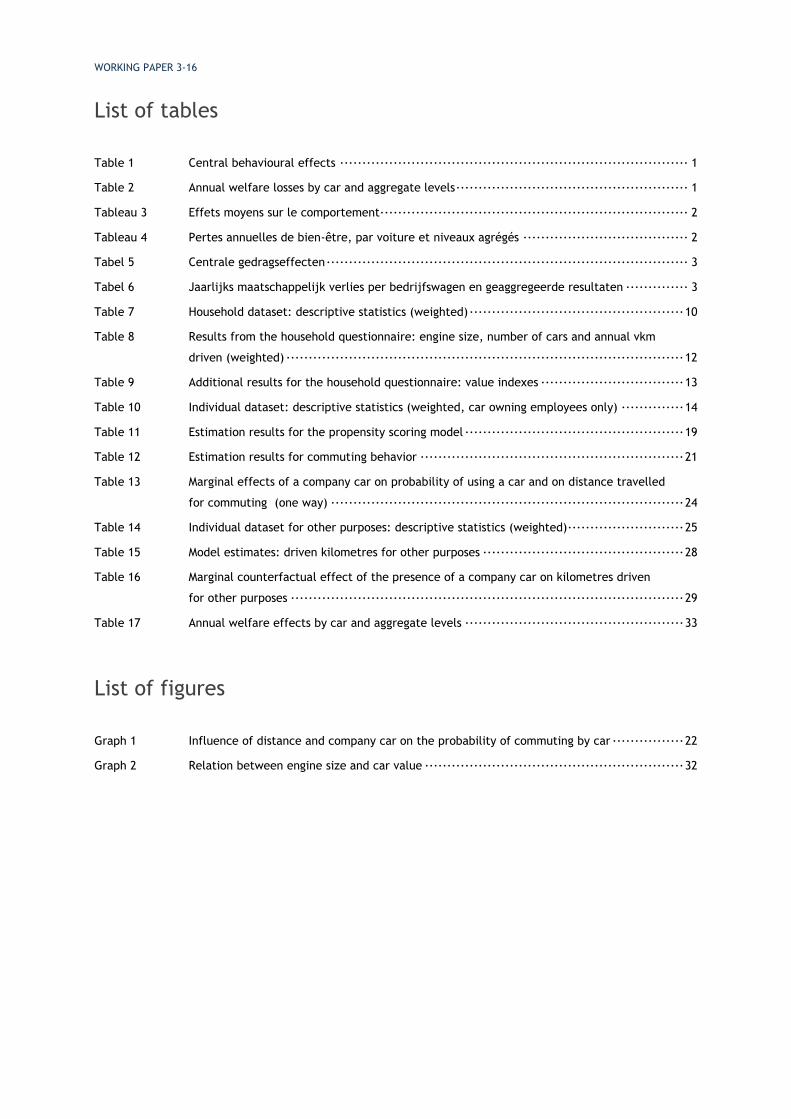
List of tables

Table 1 Central behavioural effects ·············································································· 1

Table 2 Annual welfare losses by car and aggregate levels ···················································· 1

Tableau 3 Effets moyens sur le comportement····································································· 2

Tableau 4 Pertes annuelles de bien-être, par voiture et niveaux agrégés ····································· 2

Tabel 5 Centrale gedragseffecten ················································································· 3

Tabel 6 Jaarlijks maatschappelijk verlies per bedrijfswagen en geaggregeerde resultaten ·············· 3

Table 7 Household dataset: descriptive statistics (weighted) ················································ 10

Table 8 Results from the household questionnaire: engine size, number of cars and annual vkm

driven (weighted) ························································································· 12

Table 9 Additional results for the household questionnaire: value indexes ································ 13

Table 10 Individual dataset: descriptive statistics (weighted, car owning employees only) ·············· 14

Table 11 Estimation results for the propensity scoring model ················································· 19

Table 12 Estimation results for commuting behavior ··························································· 21

Table 13 Marginal effects of a company car on probability of using a car and on distance travelled

for commuting (one way) ··············································································· 24

Table 14 Individual dataset for other purposes: descriptive statistics (weighted) ·························· 25

Table 15 Model estimates: driven kilometres for other purposes ············································· 28

Table 16 Marginal counterfactual effect of the presence of a company car on kilometres driven

for other purposes ························································································ 29

Table 17 Annual welfare effects by car and aggregate levels ················································· 33

List of figures

Graph 1 Influence of distance and company car on the probability of commuting by car ················ 22

Graph 2 Relation between engine size and car value ·························································· 32

WORKING PAPER 3-16

1

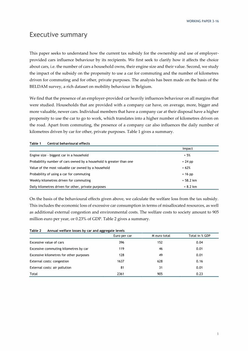
Executive summary

This paper seeks to understand how the current tax subsidy for the ownership and use of employer-

provided cars influence behaviour by its recipients. We first seek to clarify how it affects the choice

about cars, i.e. the number of cars a household owns, their engine size and their value. Second, we study

the impact of the subsidy on the propensity to use a car for commuting and the number of kilometres

driven for commuting and for other, private purposes. The analysis has been made on the basis of the

BELDAM survey, a rich dataset on mobility behaviour in Belgium.

We find that the presence of an employer-provided car heavily influences behaviour on all margins that

were studied. Households that are provided with a company car have, on average, more, bigger and

more valuable, newer cars. Individual members that have a company car at their disposal have a higher

propensity to use the car to go to work, which translates into a higher number of kilometres driven on

the road. Apart from commuting, the presence of a company car also influences the daily number of

kilometres driven by car for other, private purposes. Table 1 gives a summary.

Table 1 Central behavioural effects

Impact

Engine size - biggest car in a household + 5%

Probability number of cars owned by a household is greater than one + 24 pp

Value of the most valuable car owned by a household + 62%

Probability of using a car for commuting + 16 pp

Weekly kilometres driven for commuting + 58.2 km

Daily kilometres driven for other, private purposes + 8.2 km

On the basis of the behavioural effects given above, we calculate the welfare loss from the tax subsidy.

This includes the economic loss of excessive car consumption in terms of misallocated resources, as well

as additional external congestion and environmental costs. The welfare costs to society amount to 905

million euro per year, or 0.23% of GDP. Table 2 gives a summary.

Table 2 Annual welfare losses by car and aggregate levels

Euro per car M euro total Total in % GDP

Excessive value of cars 396 152 0.04

Excessive commuting kilometres by car 119 46 0.01

Excessive kilometres for other purposes 128 49 0.01

External costs: congestion 1637 628 0.16

External costs: air pollution 81 31 0.01

Total 2361 905 0.23

WORKING PAPER 3-16

2

Synthèse

Cette étude tente d’établir de quelle manière le régime fiscal avantageux qui s’applique actuellement à

la détention ou l’utilisation de voitures de société peut influencer le comportement des personnes qui

en bénéficient. Dans un premier temps, nous tentons de déterminer comment ce régime influence les

décisions prises par rapport au parc automobile du ménage, c’est-à-dire le nombre de voitures du mé-

nage, leur motorisation et leur valeur. Dans un deuxième temps, nous étudions l’incidence de ce régime

sur la propension à utiliser la voiture pour réaliser les déplacements domicile-lieu de travail, le nombre

de kilomètres parcourus pour ces déplacements et d’autres déplacements privés. L’analyse a été menée

par le biais de l’enquête BELDAM, qui constitue une base de données d’une grande richesse sur les

comportements en matière de mobilité en Belgique.

Nous établissons que la présence dans un ménage d’un véhicule de société influence lourdement les dif-

férents types de comportement observés. Les ménages qui disposent d’une voiture de société ont en

moyenne plus de voitures, des voitures plus grandes, plus récentes et de valeur plus élevée. Les membres

du ménage qui disposent d’une voiture de société ont davantage tendance à utiliser la voiture pour aller

travailler, ce qui se traduit par un nombre plus élevé de kilomètres parcourus sur les routes. La présence

dans le ménage d’une voiture de société influence, outre les déplacements domicile-lieu de travail, le

nombre de kilomètres parcourus à des fins privées. Le tableau 3 ci-dessous résume ces résultats.

Tableau 3 Effets moyens sur le comportement

Effets

Cylindrée de la plus grosse voiture du ménage + 5 %

Probabilité que le nombre de voitures détenues par un ménage soit supérieur à un + 24 pp

Valeur de la voiture la plus chère détenue par un ménage + 62 %

Probabilité d’utiliser la voiture pour les déplacements domicile-lieu de travail + 16 pp

Kilomètres parcourus en voiture chaque semaine pour aller travailler + 58,2 km

Kilomètres parcourus en voiture chaque jour à des fins privées + 8,2 km

Partant des effets sur les comportements décrits ci-dessus, nous calculons la perte de bien-être occasion-

née par ce régime fiscal. Cette perte englobe la perte économique liée à une détention excessive de voi-

ture et une consommation excessive des services de transport produits par ces voitures. Cette mauvaise

affectation des ressources s’accompagne de coûts environnementaux et de congestion externes addi-

tionnels. Les coûts liés à la perte de bien-être représentent 905 millions d’euros par an, soit 0,23 % du

PIB. Le tableau 4 résume les effets sur le bien-être.

Tableau 4 Pertes annuelles de bien-être, par voiture et niveaux agrégés

Euros par voiture M euros au total Total en % du PIB

Excès dans la valeur des voitures 396 152 0,04

Excès dans les kilomètres en voiture pour les déplacements

domicile-travail

119 46 0,01

Excès dans les kilomètres en voiture pour d’autres motifs 128 49 0,01

Coûts externes : congestion 1637 628 0,16

Coûts externes : pollution de l’air 81 31 0,01

Total 2361 905 0,23

WORKING PAPER 3-16

3

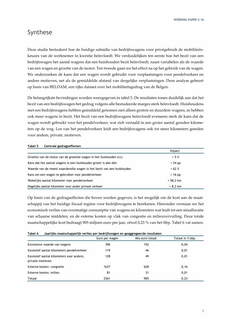
Synthese

Deze studie bestudeert hoe de huidige subsidie van bedrijfswagens voor privégebruik de mobiliteits-

keuzes van de werknemer in kwestie beïnvloedt. We verduidelijken ten eerste hoe het bezit van een

bedrijfswagen het aantal wagens dat een huishouden bezit beïnvloedt, naast variabelen als de waarde

van een wagen en grootte van de motor. Ten tweede gaan we het effect na op het gebruik van de wagen.

We onderzoeken de kans dat een wagen wordt gebruikt voor verplaatsingen voor pendelverkeer en

andere motieven, net als de gemiddelde afstand van dergelijke verplaatsingen. Deze analyse gebeurt

op basis van BELDAM, een rijke dataset over het mobiliteitsgedrag van de Belgen.

De belangrijkste bevindingen worden weergegeven in tabel 5. De resultaten tonen duidelijk aan dat het

bezit van een bedrijfswagen het gedrag volgens alle bestudeerde marges sterk beïnvloedt. Huishoudens

met een bedrijfswagens hebben gemiddeld genomen niet alleen grotere en duurdere wagens, ze hebben

ook meer wagens in bezit. Het bezit van een bedrijfswagens beïnvloedt eveneens sterk de kans dat de

wagen wordt gebruikt voor het pendelverkeer, wat zich vertaald in een groter aantal gereden kilome-

ters op de weg. Los van het pendelverkeer leidt een bedrijfswagens ook tot meer kilometers gereden

voor andere, private, motieven.

Tabel 5 Centrale gedragseffecten

Impact

Grootte van de motor van de grootste wagen in het huishouden (cc) + 5 %

Kans dat het aantal wagens in een huishouden groter is dan één + 24 pp

Waarde van de meest waardevolle wagen in het bezit van een huishouden + 62 %

Kans om een wagen te gebruiken voor pendelverkeer + 16 pp

Wekelijks aantal kilometer voor pendelverkeer + 58,2 km

Dagelijks aantal kilometer voor ander privaat verkeer + 8,2 km

Op basis van de gedragseffecten die boven werden gegeven, is het mogelijk om de kost aan de maat-

schappij van het huidige fiscaal regime voor bedrijfswagens te berekenen. Hieronder verstaan we het

economisch verlies van overmatige consumptie van wagens en kilometers wat leidt tot een misallocatie

van schaarse middelen, en de externe kosten op vlak van congestie en milieuvervuiling. Deze totale

maatschappelijke kost bedraagt 905 miljoen euro per jaar, ofwel 0,23 % van het bbp. Tabel 6 vat samen.

Tabel 6 Jaarlijks maatschappelijk verlies per bedrijfswagen en geaggregeerde resultaten

Euro per wagen Mio euro totaal Totaal in % bbp

Excessieve waarde van wagens 396 152 0,04

Excessief aantal kilometers pendelverkeer 119 46 0,01

Excessief aantal kilometers voor andere,

private motieven

128 49 0,01

Externe kosten: congestie 1637 628 0,16

Externe kosten: milieu 81 31 0,01

Totaal 2361 905 0,23

WORKING PAPER 3-16

4

1. Introduction

This paper seeks to shed light on the welfare effects of the current tax rules for company car taxation in

Belgium, using the data from the BELDAM survey, a rich survey on Belgians’ mobility behaviour. It is

well known that company cars in Belgium enjoy a substantial tax advantage vis-a-vis ordinary wages.

Harding (2014) calculates the average tax expenditure for a typical car for all OECD countries, and finds

that company cars in Belgium enjoy the largest tax advantage among European countries: 2 763 euro

per car.

The result of this policy is that Belgians on average use more company cars than ever. The fleet is esti-

mated at 383 400 company cars1, which are intensively used during the peak period on workdays. In-

deed, estimates by SD Worx even put the share of company cars during Brussels’ rush hour at 50%.

Moreover, most company cars are diesel cars, which are known to have higher emissions of damaging

particulate matter and NOx. They thus are likely to contribute to the already high cost of congestion

and local air pollution.

Maintaining this subsidy scheme makes other government policy for controlling externalities difficult.

De Borger and Wuyts (2011), for example, seek to quantify the impact of company cars on the congestion

problem and find that optimal congestion tolls should be set much higher than standard theory would

prescribe, if the use of company cars continues to be highly subsidised by the personal income tax sys-

tem. Apart from hampering efficiency, this raises equity issues as well. Indeed, if the government needs

to impose a high congestion charge to compensate for the company car subsidy scheme, it may impose

an unduly high costs on people having no access to a company car.

Nonetheless, the work of De Borger and Wuyts (2011) may be based on strong assumptions with respect

to behaviour: in their model, owners of company cars are always assumed to use the car, while those

without are assumed to follow the modal split between public and car transport that is observed by the

general population in the baseline scenario. They do not allow for the possibility that owners of com-

pany cars may have a higher propensity to use a car, even without the tax subsidy. Also, they only

consider the impact of company cars on commuting trips, while ignoring the potential impact on trips

for other purposes.

To fully understand the economic and environmental impact of company cars, we need to understand

the impact of the fiscal treatment on behaviour along different behavioural margins. Ideally, we should

be able to distinguish the impact on the number of cars in the household, the size or market value of the

cars and the number of vehicle kilometres driven for different purposes.

Until now, empirical research on company car use in Belgium has been scarce. The only detailed studies

that we know of, have been done by Ramaekers etal. (2010) and De Witte and Macharis (2010 & 2012).

1 A microsimulation exercise performed for us by Federal Public Service Finance revealed that in 2011, 383 400 tax returns had

a positive value for the taxable benefit for an employer-provided company car. This may be underestimate due to the fact

that couple can also file a joint tax return. This figure, which will be used in this paper, lies well below the 722 000 based on

car registrations by Harding (2014), but above the 365 000 for the 4th quarter of 2011 from the social security administration.

WORKING PAPER 3-16

5

Using a multivariate regression analysis, the former finds a difference of 9 200 kilometres driven be-

tween those with and those without a company car. De Witte and Macharis (2012) suggest different

behavioural impacts for various types of company car users. In an earlier study, De Witte and Macharis

(2010) found strong effects of company car possession on the propensity to use the train by commuters

to Brussels.

Other research abroad includes work done regarding Israel by Shiftan, Albert and Keinan (2012), who

find that a company car increases the amount of kilometres driven by 3 000 to 10 000 km per year, de-

pending on whether a fuel card and free parking are included in the compensation package. For the

Netherlands and Germany, Kloosterboer (2012) found strong effects of company cars on modal choice,

with public transport losing market share in the Netherlands. In Germany, however, no effect was

found.

Gutierrez and Van Ommeren (2011) provide the most detailed analysis of behavioural reactions yet.

They studied the effect of owning a company car on the value of cars in the household, the commuting

distance and the number of daily kilometres driven for private, non-commuting purposes. Using di-

verse panel datasets for the Netherlands, they found large effects on car values, but relatively modest

effects on the commuting distance and kilometres driven. In their study, the value of the most expensive

car in the household is inflated by about 10 000 euro when it is a company car. As for car use, private

weekend travel is increased by 3 km and total commuting distance, regardless of the mode taken is

increased by 5 km per day.

Some surveys ask people directly how abolishing the company car regime would alter their mobility

behaviour. For Belgium, for example, about 20% of current users state they would switch to another

mode of transport (mainly rail) if they had no company car at their disposal. This effect is most pro-

nounced for females. (Cornelis e.a., 2011b) A survey conducted in Israel by Shiftan et al. (2011) states

that half of company car users would still stick to their own privately owned car as the main mode of

commuting.

The purpose of this paper is to quantify the different effects of company car taxation on different deci-

sion variables, so as to be able to provide a full picture of the societal costs of the preferential tax treat-

ment of company cars. In order to do this, we follow the method of Gutierrez and Van Ommeren (2011),

which relies on survey data to quantify the tax distortion for the Netherlands.

We calculate the effect of company car possession on average engine size, the number of cars, and the

car value per household, alongside car use. Within car use, we distinguish between commuting and

other purposes. For car use, we implement econometric models that are able to distinguish between

modal choice and the amount of kilometres driven per trip, exploring the use of double hurdle models

for transport analysis alongside standard discrete choice models.

After calculating behavioural effects, we also provide an estimate of the societal loss from company car

subsidies. This is done not only by calculating the standard economic welfare loss from excessive con-

sumption through product subsidies, but also by providing an estimate of the additional external costs

from induced car use. Both congestion costs and environmental costs are considered.

WORKING PAPER 3-16

6

2. Theoretical framework

Gutierrez and Van Ommeren (2011) provide a framework for estimating the distortion from company

car taxation. Using simplifying assumptions, a tractable equation is derived from the utility maximisa-

tion of an employer deciding to offer a company car or not.

A household without a company car is assumed to maximise utility 𝑈 defined over two goods: car ‘units’

𝑥 and other goods 𝑦. Car ‘units’ can be understood as anything that makes a car desirable: engine size,

extra facilities or the mileage that is driven with it. Note that mileage is understood as being for private

car use, commuting and other purposes but not for work-related travel.

The price of the good y is normalised to 1, that of cars is 𝑝. Gross income 𝑚 is taxed at rate 𝜏. The maxi-

malisation problem is thus:

𝑚𝑎𝑥𝑥,𝑦𝑈(𝑥, 𝑦)

𝑠. 𝑡. 𝑝𝑥 + 𝑦 = 𝑚(1 − 𝜏)

or:

𝑚𝑎𝑥𝑥 𝑈(𝑥, 𝑚(1 − 𝜏) − 𝑝𝑥))

This yields a first order condition:

𝑈𝑥𝑈𝑦

⁄ = 𝑝

and a demand curve for car units:

𝑥 = 𝑥(𝑝, 𝑚(1 − 𝜏))

Households with access to a company car solve a similar problem. The main difference is that the in-

come from a company car is taxed differently from other income. More precisely, a unit of company

cars 𝑥𝑐 is valued by the tax administration at 𝐻 ≤ 𝑝. Their problem is:

𝑚𝑎𝑥𝑥𝑐,𝑦𝑈(𝑥𝑐 , 𝑦)

𝑠. 𝑡. 𝑝𝑥𝑐 + 𝑦 = 𝑚𝑐(1 − 𝜏) − 𝜏𝐻𝑥𝑐 + 𝑝𝑥𝑐

or:

𝑚𝑎𝑥𝑥 𝑈(𝑥𝑐 , 𝑚𝑐 − 𝜏(𝑚𝑐 + 𝐻𝑥𝑐))

Firms wish to maximise revenue by offering a package of company cars 𝑥𝑐 and money wages 𝑚𝑐, such

that employees would be indifferent as to whether they have a company car or not. This implies:

𝑈(𝑥, 𝑚𝑐 − 𝜏(𝑚𝑐 + 𝐻𝑥𝑐)) = 𝑈(𝑥, 𝑚(1 − 𝜏) − 𝑝𝑥))

WORKING PAPER 3-16

7

When company cars do not yield any benefit to the firm2, the result of the firm’s maximisation problem

is:

𝑈𝑥𝑐

𝑈𝑦⁄ = 𝑝 − 𝜏(𝑝 − 𝐻) = 𝑝𝑐

This equation is important, since it shows that the relevant price to the household is the market value

of a company car unit less the tax subsidy, i.e. the difference between the market value and the value

assumed by the tax system, evaluated at the marginal income tax rate. If 𝐻 equals 𝑝, there is no distor-

tion from the tax system, and the number of car units demanded by households that own a company

car 𝑥𝑐 is equal to that demanded by households without a company car 𝑥. When 𝐻 < 𝑝, the tax subsidy

rises proportionally to the tax rate, so that the tax subsidy rate not only depends on the realism of the

imputed value 𝐻, but also on the reference marginal tax rate.

In reality, 𝑥𝑐 and 𝑥 will not be equal. This may be due to different household characteristics as well as

the tax treatment of company cars. Empirical work must thus isolate the latter effect from other charac-

teristics.

This can easily be done if demand functions of households 𝑖 are assumed to be additive:

𝑥𝑖 = ℎ(𝑝𝑖) + 𝑘(𝑚𝑖) + 𝑗(𝑠𝑖)

Where 𝑝𝑖 is the price for a car unit corrected for the income tax treatment (𝑝𝑐 for households with a

company car, 𝑝 for one without), 𝑚𝑖 is money income and 𝑠𝑖 are other important household character-

istics.

Differences in demand for car units between households with or without a company car can be ex-

pressed as:

∆𝑥𝑖 = 𝑥𝑖 − 𝑥𝑖𝑐 = ℎ(𝑝) − ℎ(𝑝𝑐) + 𝑘(𝑚𝑖) − 𝑘(𝑚𝑖

𝑐) + 𝑗(𝑠𝑖) − 𝑗(𝑠𝑖𝑐)

Empirical work should estimate the magnitude of the first difference on the right hand side ∆𝑥 = ℎ(𝑝) −

ℎ(𝑝𝑐). It is the demand change induced by the preferential tax rules on company cars, controlling for

changes in income.

The welfare losses to society equal the changes in consumer surplus ∆𝐶𝑆 and environmental cost ∆𝐸𝐶.

The change in consumer surplus ∆𝐶𝑆 can be captured by the simple deadweight loss formula of a linear

demand curve:

∆𝐶𝑆 = 1/2∆𝑝

𝑝⁄ ∆𝑥

In the context of a subsidy, this deadweight loss can be understood as the loss to society due to excessive

consumption of the good in question. Because the subsidy distorts relative prices, consumers are in-

duced to buy a different bundle of goods compared to the situation in which prices are not affected by

government policy.

2 We will assume this is the case throughout the analysis.

WORKING PAPER 3-16

8

The term ∆𝐶𝑆 represents the loss to society due to this misallocation of resources. Intuitively, it is the

gain to consumers when the subsidy is abolished and they receive the revenue back in freely disposable

cash, which would allow them to buy a bundle of good that is closer to their preferences.

In the context of our study, we consider the excessive consumption of car units, i.e. the number and

value of cars, and the number of vehicle km driven by them for commuting and other (private) pur-

poses.

To arrive at complete welfare effects, one also needs to consider the effects on external costs ∆𝐸𝐶:

∆𝐸𝐶 = ∆𝑥(𝑀𝐸𝐸𝐶 + 𝑀𝐸𝐶𝐶)

𝑀𝐸𝐸𝐶 and 𝑀𝐸𝐶𝐶 are marginal external environmental and marginal external congestion costs, respec-

tively.

WORKING PAPER 3-16

9

3. Empirical results

3.1. Data

Identifying the effect of company cars’ preferential tax rules on the demand for car units, controlling for

income and household characteristics, requires microdata rich enough to encompass the socio-eco-

nomic, fiscal and mobility aspects involved. This kind of data is unfortunately not abundant for Bel-

gium. Several promising datasets, such as the Labour Force Survey, or the decennial (micro) census

datasets, miss one or other critical piece of information required for the analysis. In particular, microdata

that explicitly includes information about the availability and use of a company car in a household is

scarce. Though the development of relevant microdata based on administrative registers is possible, the

situation in that respect is not yet mature in Belgium, and we hence have resorted to an alternative

solution: the BELDAM (BELgian DAily Mobility) survey.

BELDAM is a sampled cross-sectional survey, carried out in 2010, and covering the population of Bel-

gian residents. The sample consists of some 8 500 households that represent more than 15 800 individ-

uals aged six or more. Though response rates vary across segments of the population, this survey is

sufficiently large and correctly weighted to be considered as representative of the Belgian population

for our purpose, with known caveats.

The first questionnaire in the survey addresses general characteristics such as household income, the

educational and professional status of each household member and many other useful control variables.

It also provides detailed information on the number of vehicles owned by the household and their char-

acteristics, including whether they are a company car. It includes aggregate use data in the form of

kilometers driven per year, regardless of purpose.

The second questionnaire is individual, and includes each person in the household aged six or more,

for whom a number of items regarding regular mobility behavior and a trip log for a randomly selected

day during the survey period are reported. The first part of this questionnaire addresses, among other

matters, commuting behavior to work or school, providing information on the transport modal chain,

distances and the weekly pattern. It does not directly specify whether car trips are made with a company

car or not, but this information can be inferred from a question related to the way commuting expenses

are covered by the employer. The second part of the questionnaire provides detailed information for all

trips occurring on the selected day, including distance, time and mode for each leg of each trip, purposes

of the trips and, if applicable, which of the household’s cars was used. This last piece of information

allows identification of whether car trips are made with a company car.

This rather rich dataset is the basis of several econometric analyses, whose description unfolds in the

following sections. The household questionnaire is exploited first, linking the presence of a company

car to overall car ownership and usage by the household. Car usage by purpose is then explored in more

depth using the individual questionnaire, with separate treatment of car usage for work commuting

and for other purposes.

WORKING PAPER 3-16

10

3.2. Overall results: the household questionnaire

Ideally, in this initial analysis we would explore the link between the value of the household’s cars and

the presence of a company car. However, the crucial variable on the value of the car at purchase that

was available to Gutierrez and Van Ommeren (2011) is missing from our survey data. We shall therefore

use a proxy based on the car characteristics available to us. The best candidate in this respect is the

engine displacement in cubic centimeters (CC)3. Additional information on car units is in the age of the

car. From this data, a depreciation can be inferred, to better reflect the market value of the car at the

survey date. This will, among other things, capture the fact that company cars are renewed much more

frequently than privately owned cars. This car value index is defined as the car’s engine displacement,

depreciated at a rate of 15% per year. This rate seems a reasonable average of estimations in interna-

tional studies on second-hand car markets. The household questionnaire allows us therefore to estimate

the effects of a company car on engine displacement and the car value index. This can be seen as a

(rough) measure of ‘car units’ in the model presented in section 2. Likewise, the extra number of yearly

vehicle kilometres driven by company cars can be estimated, as an additional use-based measure of ‘car

units’.

Table 7 below provides some descriptive statistics for the subsample of households owning at least one

car. From the consideration of sample standard deviations, we can conclude that for the subsample of

households owning a company car, car characteristics and usage are more homogeneous than for the

subsample of households without a company car. In the dataset, when the biggest car is a company car,

its engine displaces on average 12% more CC, and its value index is 70% higher. The total number of

yearly vkm driven in a household is 109% higher if at least one company car is present. 74% of house-

holds that own a company car have 2 cars or more, as opposed to only 33% of other households. A

regression analysis should determine whether this also holds when controlling for important household

characteristics such as income, household composition, etc.

Table 7 Household dataset: descriptive statistics (weighted)

Engine size biggest car (CC) Share of

HH +1 cars

Annual mileage (vkm) Highest car value index

Mean SD Mean SD Mean SD

Whole sample 1781.8 455.4 38.0% 19109.4 25638.8 834.5 514.1

Company car 1970.7 360.8 74.5% 35907.9 23913.2 1314.7 450.8

No company car 1758.7 460.5 33.8% 17147.3 25114.6 773.5 489.0

N 5636 6427 6427 5420

As for car characteristics and the number of cars, we estimate in turn 1) the effect of company car own-

ership on the engine size of the largest car in the household or alternatively on the highest value index

car, 2) the effect of the presence of a company car on the probability that the household has at least two

cars or more and 3) the effect of the presence of a company car on the total number of CCs owned by a

household. The results are reported in Table 8 and Table 9 below. The second analysis is performed

through a logistic regression.

3 In section 4 we illustrate the tight link between car value and engine displacement, showing that on a log-scale, there is a

strong linear relationship, with log-value of cars behaving like 1.3 times log-displacement of engines.

WORKING PAPER 3-16

11

The results indicate that, among households that own a car, the engine size of the largest car in the

household is 5% larger for those owning a company car. The value index of the car with highest value

is 61% larger for households where the highest value car is a company car. This very significant differ-

ence is statistically robust, and still below the effect estimated by Gutierrez and Van Ommeren (between

0.8 and 1.2 in logarithm, thus between 122% and 230%). However, the car valuation method used by

these authors gives a large premium to cars under three years of age, a category that contains 75% of

company cars4. The parameters of the logistic regression imply that for households with a company car,

the probability of having two or more cars is 24 percentage points (pp) higher than for households

without company car. The third regression shows that the total number of ccs owned by a household

with a company car is 15% higher. Finally, the sum of value indexes of all cars in the household is

estimated to be 68% higher for households with at least one company car. All relevant coefficients are

highly significant, implying a marked effect of subsidies on car choice.

Also noteworthy is the effect of household income, composition and location. As expected, income has

a strong positive effect on engine size, car value and the number of cars in the household. It is a highly

significant predictor of both margins, more so than the education and employment status of the head

of the household (regressions that include these variables are not shown).

In the fourth column of table 8, we report the effect of company car ownership on total vehicle kilome-

tres driven by a household. The estimated coefficient implies that abolishing the company car regime

would diminish vkm driven by households with a company car by 34% or about 12 077 vkm per year.

Again, income, household composition and location of residence are highly significant. Age has a neg-

ative impact on kilometers driven; the presence of children in the household seems to have a positive

effect.

4 Gutierrez & Van Ommeren (2011) attribute to cars less than three years old their new listed price, and for older cars, a second-

hand market value. As company cars are always bought new, the retained value for such cars is the new value, whereas it is

well established that depreciation is high in the first year for cars. This therefore probably distorts estimates of the difference

in car value between company and privately owned cars, overstating that difference.

WORKING PAPER 3-16

12

Table 8 Results from the household questionnaire: engine size, number of cars and annual vkm driven (weighted)

H1

Log cc biggest car

(OLS)

H2

Probability number

cars > 1 (Logistic)

H3

Log total cc’s owned

by a household (OLS)

H4

Log total annual vkm

(OLS)

At least 1 company car in HH 0.24***(7.89) 0.14***(8.10) 0.41***(11.94)

Biggest car = company car 0.05***(4.65)

Log age head of household -0.06***(-5.42) -0.16***(-7.12) -0.15***(-7.73) -0.83***(-21.31)

Income = 500-999 euro/month -0.00 (-0.01) -0.23***(-14.82) -0.23***(-2.91) -0.05 (-0.33)

Income = 1000-1499 euro/month 0.02 (0.53) -0.26***(-8.19) -0.19**(-2.50) -0.03 (-0.22)

Income = 1500-1999 euro/month 0.07 (1.57) -0.23***(-4.73) -0.11 (-1.47) 0.06 (0.42)

Income = 2000-2499 euro/month 0.08* (1.90) -0.19***(-4.97) -0.08 (-1.07) 0.17 (1.17)

Income = 2500-2999 euro/month 0.10** (2.28) -0.15***(-3.19) 0.00 (0.05) 0.20 (1.37)

Income = 3000-3999 euro/month 0.09** (2.09) -0.11* (-1.86) 0.03 (0.48) 0.32**(2.19)

Income = 4000-4999 euro/month 0.15***(3.23) -0.01 (-0.17) 0.17**(2.24) 0.44***(2.99)

Income = 5000-9999 euro/month 0.22***(4.69) 0.09 (0.89) 0.30***(3.73) 0.66***(4.27)

Income = 10000+ euro/month 0.43***(6.73) 0.21 (1.04) 0.52***(4.72) 0.81***(3.86)

Gender head HH = female -0.07***(-10.01) 0.02 (1.33) -0.07***(-5.75) -0.13***(-4.82)

Urbanisation level = 2 0.03***(4.21) 0.17***(8.30) 0.11***(7.94) 0.13*** (4.49)



Region = Flanders 0.03**(2.09) 0.07**(2.18) 0.05**(2.15) 0.16***(3.82)

Region = Wallonia -0.01 (-0.72) 0.11***(4.05) 0.04*(1.73) 0.35***(8.15)

Renter -0.04***(-4.94) -0.11***(-7.45) -0.10***(-7.16) -0.07** (-2.40)

Other residence -0.06*** (-2.86) 0.05 (1.01) -0.07 (-1.82) -0.10 (-1.36)

Two adults 0.04*** (5.31) 0.30***(20.96) 0.19***(13.71) 0.18***(6.35)

Children in HH 0.02*** (3.08) 0.11***(7.46) 0.09*** (7.37) 0.17***(7.01)

Constant 7.56*** (118.91) 8.04***(73.91) 12.26***(57.33)

N 5275 6342 5548 5275

R² 0.17 0.33 0.34 0.32

t statistic in parentheses. *** denotes significance at level 0.01, ** at level 0.05, * at level 0.10. For the logistic regression, we report marginal effects at means and the pseudo-R² The subsample includes only households that own at least one car. Model H4 only considers households with a non-null total annual vkm.

WORKING PAPER 3-16

13

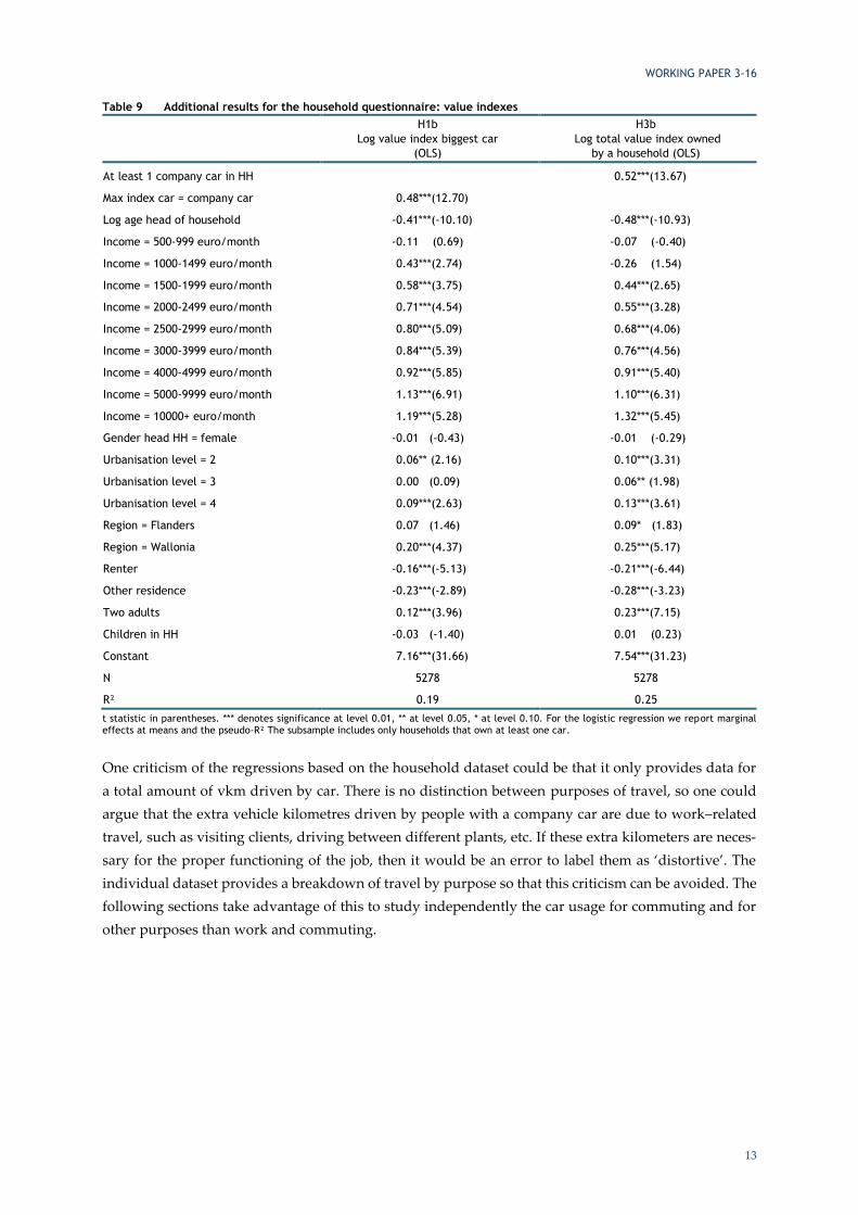
Table 9 Additional results for the household questionnaire: value indexes

H1b

Log value index biggest car

(OLS)

H3b

Log total value index owned

by a household (OLS)

At least 1 company car in HH 0.52***(13.67)

Max index car = company car 0.48***(12.70)

Log age head of household -0.41***(-10.10) -0.48***(-10.93)

Income = 500-999 euro/month -0.11 (0.69) -0.07 (-0.40)

Income = 1000-1499 euro/month 0.43***(2.74) -0.26 (1.54)

Income = 1500-1999 euro/month 0.58***(3.75) 0.44***(2.65)






Income = 10000+ euro/month 1.19***(5.28) 1.32***(5.45)

Gender head HH = female -0.01 (-0.43) -0.01 (-0.29)

Urbanisation level = 2 0.06** (2.16) 0.10***(3.31)

Urbanisation level = 3 0.00 (0.09) 0.06** (1.98)

Urbanisation level = 4 0.09***(2.63) 0.13***(3.61)

Region = Flanders 0.07 (1.46) 0.09* (1.83)

Region = Wallonia 0.20***(4.37) 0.25***(5.17)

Renter -0.16***(-5.13) -0.21***(-6.44)

Other residence -0.23***(-2.89) -0.28***(-3.23)

Two adults 0.12***(3.96) 0.23***(7.15)

Children in HH -0.03 (-1.40) 0.01 (0.23)

Constant 7.16***(31.66) 7.54***(31.23)

N 5278 5278

R² 0.19 0.25

t statistic in parentheses. *** denotes significance at level 0.01, ** at level 0.05, * at level 0.10. For the logistic regression we report marginal effects at means and the pseudo-R² The subsample includes only households that own at least one car.

One criticism of the regressions based on the household dataset could be that it only provides data for

a total amount of vkm driven by car. There is no distinction between purposes of travel, so one could

argue that the extra vehicle kilometres driven by people with a company car are due to work–related

travel, such as visiting clients, driving between different plants, etc. If these extra kilometers are neces-

sary for the proper functioning of the job, then it would be an error to label them as ‘distortive’. The

individual dataset provides a breakdown of travel by purpose so that this criticism can be avoided. The

following sections take advantage of this to study independently the car usage for commuting and for

other purposes than work and commuting.

WORKING PAPER 3-16

14

3.3. Commuting by car: the individual questionnaire

The empirical framework

The individual dataset allows us to reconstruct daily commuting patterns of employees on a detailed

basis. It provides information on the length of the itinerary towards work that is usually followed, bro-

ken down by mode. Also, the number of days that is usually spent working per week is given. This

allows us to deduce the number of kilometers spent commuting by car in a typical workweek. The

questionnaire also provides a few other controls that might influence the results, namely the sector

(public vs private vs non-profit), work schedule (flexible, shifts, etc.), the number of hours worked (full-

time vs part-time), some accessibility parameters (ease of parking near home and near the workplace,

proximity of public transport to home location), and, of course, characteristics derived from the house-

hold questionnaire (household monthly income, individual education level and a crude measure of the

type of job, region of residence and urbanisation category of the district of residence).

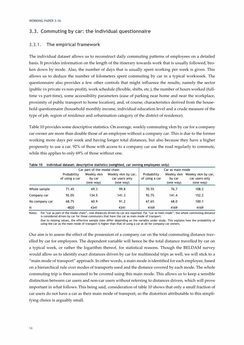
Table 10 provides some descriptive statistics. On average, weekly commuting vkm by car for a company

car owner are more than double those of an employee without a company car. This is due to the former

working more days per week and having longer total distances, but also because they have a higher

propensity to use a car. 92% of those with access to a company car use the road regularly to commute,

while this applies to only 69% of those without one.

Table 10 Individual dataset: descriptive statistics (weighted, car owning employees only)

Car part of the modal chain Car as main mode

Probability

of using a car

Weekly vkm

by car

(one way)

Weekly vkm by car,

car users only

(one way)

Probability

of using a car

Weekly vkm

by car

(one way)

Weekly vkm by car,

car users only

(one way)

Whole sample 71.4% 69.3 99.8 70.5% 76.7 108.2

Company car 92.0% 134.5 141.3 92.7% 141.4 152.2

No company car 68.7% 60.9 91.2 67.6% 68.0 100.1

N 4820 4341 4341 4169 4169 4169

Notes: For “car as part of the modal chain”, real distances driven by car are reported. For “car as main mode”, the whole commuting distance is considered driven by car for those commuters that have the car as main mode of transport.

Due to missing values, the effective sample sizes differ depending on the variable under study. This explains how the probability of using the car as the main mode of transport is higher than that of using a car at all for company car owners.

Our aim is to assess the effect of the possession of a company car on the total commuting distance trav-

elled by car for employees. The dependent variable will hence be the total distance travelled by car on

a typical week, or rather the logarithm thereof, for statistical reasons. Though the BELDAM survey

would allow us to identify exact distances driven by car for multimodal trips as well, we will stick to a

“main mode of transport” approach. In other words, a main mode is identified for each employee, based

on a hierarchical rule over modes of transports used and the distance covered by each mode. The whole

commuting trip is then assumed to be covered using this main mode. This allows us to keep a sensible

distinction between car users and non-car users without referring to distances driven, which will prove

important in what follows. This being said, consideration of table 10 shows that only a small fraction of

car users do not have a car as their main mode of transport, so the distortion attributable to this simpli-

fying choice is arguably small.

WORKING PAPER 3-16

15

The total distance travelled by car depends on two main factors: the modal choice of the commuter, and

the distance between the place of residence and the place of work. The presence of a company car may

have an influence on both factors.

Regarding the modal choice, the presence of an all-expenses-paid car of a quality probably higher than

that which the household would have chosen if they had paid for it themselves (as demonstrated in the

previous section) is an incentive to choose commuting by car. It may also happen that, having provided

the employee with a company car, the employer does not cover expenses linked with other modal

choices, such as train tickets or an urban transport travel pass. In that case, the choice of car would also

be the favoured alternative on a cost basis. Hence we expect that the presence of a company car would

increase the probability of commuting by car. But other factors, such as the commute distance, other

constraints (children, unusual working hours at odds with public transport time schedules, residence

in a poorly connected area, personal preferences that may correlate with age, gender or other observable

characteristics, etc.) also impact the modal choice of commuters. This means that a broad regression

model has to be specified to estimate this impact.

Regarding the distance between place of residence and place of work, the link with the presence of a

company car is less obvious at first, but also more complex to specify correctly. On the one hand, on

condition of being provided with an all-expense-paid company car, individuals could accept jobs fur-

ther away from their home than they would have done without being offered a car. In this respect, the

presence of a company car could, on average, have a positive causal effect on the job-home distance and

the total kilometers driven. On the other hand, workers with long commutes (e.g. living in remote areas

or interested in job positions only available at potentially distant specific locations such as airports,

harbours or capital cities) may specifically select jobs for which company cars are provided, to ease the

commuting burden. In that case, the causal relation is inverted, and longer commuting distances imply,

by selection, a higher chance of registering a company car in the household.

We do not seek a comprehensive model for an agent’s decision on mode and commuting distance that

would structurally address these uncertainties. Such a model would, among other characteristics, re-

quire specific company car attribution modeling, which is the subject of further research that extends

far beyond the informational content of our data source. We rather focus on providing an estimate of

the impact on kilometers driven of the hypothetic abrogation of the specific fiscal treatment of company

cars5. To this aim, we do not necessarily need a fully-fledged structural model behind agents’ decision

processes, but can work with some reduced-form econometric model as long as endogeneity issues ap-

pear manageable. This model will provide an insight into the causal relation between the presence of a

company car and number of kilometers driven, conditional on a series of control variables, as evidenced

by our data source. To specify such a model, a qualitative consideration of the decision mechanism at

work is nonetheless required, allowing us to propose a relevant functional form and a coherent selection

of covariates. In what follows, we first deduce an appropriate econometric model specification from

qualitative considerations regarding the demand mechanism for kilometers driven by car for commut-

ing, and then discuss on this basis the endogeneity issues that may arise. The estimation results conclude

this section.

5 Using the formal vocabulary of treatment impact analysis, we seek an estimate of the (average) treatment effect on the treated,

or (A)TT.

WORKING PAPER 3-16

16

Model specifications

Distances driven by car for commuting purposes are not a direct decision by employees, but rather a

consequence or a part of their labour market decisions. Agents maximise their net utility derived from

work by balancing the income and cost consequences of accepting a specific job. Commuting cost is one

among many aspects considered. This cost obviously depends on the job location and the place of resi-

dence of the worker, which determine the commuting distance. But it also depends on the job’s accessi-

bility in a broader sense: availability of public transport close to home and work, ease of parking close

to home and work, compatibility of the job’s time schedule with the public transport offering, provision

of transportation means by the employer and other similar characteristics which have an impact on the

generalised cost of commuting; that is, the cost in both time and monetary dimensions. The choice of a

commuting mode is an integral part of the optimisation program of the worker when faced with a job

opportunity in that it influences the generalised cost of commuting. All in all, one has to consider that,

in making decisions about the job market, workers simultaneously choose a professional occupation, a

commuting distance and the main mode of transport. This decision depends on job characteristics,

household characteristics and transport-related variables.

As a consequence, for our empirical work, observed demand for distances driven by car in the commut-

ing context can be considered ex post as a simultaneous decision regarding using a car, and how far to

drive it, depending on the aforementioned characteristics. Although the underlying decision process

diverges from the optimal choice problem for usual consumption goods, this strongly relates to the

“participation decision/amount of consumption decision” framework of double hurdle models, which

have been widely used in the consumer demand literature (see e.g. Deaton 1986). Application of such

models to transport demand is still limited; but notably, Tsekeris & Dimitriou (2008) use such a frame-

work to study demand for public transportation in Greece, and Eakins (2016) uses such models to study

the demand for car fuels in Ireland. This type of model provides a flexible specification to accommodate

the presence of numerous zero observations in the response variable, arising in our case when the modal

choice for commuting is not the car.

The general idea behind these models revolves around two concepts: truncation and the separation of

different aspects of the decision making in the modeling process. Truncation relates to the fact that con-

sumption is positive, and hence bounded by zero below. Linear consumption equations must hence be

truncated at zero. This leads to the archetypical Tobit (Tobin, 1953) model. The separation of different

aspects in the decision making typically distinguishes between the decision to consume a given good at

all and the choice of the amount to consume. That would be, in our case, the decision to commute by

car, and the distance to commute. In the models based on this rationale, the observation of zero con-

sumption may then have several sources: either the household is not willing to consume the good at all,

for non-economic reasons (participation decision), or the household is willing to consume the good, but

economic considerations produce a corner solution and the household demand is null (consumption

decision). Both decisions can be related to different but overlapping sets of explanatory factors. This

framework involving two adequately modelled causes for observing null consumption provides much

safer theoretical ground for building econometric models fitting the data than a simple linear demand

equation.

WORKING PAPER 3-16

17

The first source of zero observation implies a binomial outcome variable (participation or not), which is

typically related to Probit or Logit models when considered on its own. The second source of zero ob-

servations relates to truncation, and by itself points toward Tobit models. When considered simultane-

ously, these two sources of zero observation lead to the concept of double hurdle models. These models

consider the two aspects simultaneously, and provide a unified and coherent econometric framework

to estimate their features. Tsekeris & Dimitriou (2008) give a good account of the historic development

of multiple hurdle models in this situation, while one may refer to Humphreys (2013) for a survey of

associated econometric approaches. We will make use of this kind of model here, while keeping the

simpler Probit model as a useful alternative (modeling the participation decision only) should the mod-

eling of distance between job and residence locations prove inadequate.

In the case of work commuting modeling, one might more precisely argue in favour of a “first hurdle

dominance” model within the broader family of double hurdle models. Such models assume that all

households participating will have a strictly positive consumption. In our case, “participating” refers to

choosing the car as the main mode of transport for commuting purposes, and as our sample consists

only of employed individuals working at a fixed location outside the home, the commuting distance is

always positive, hence “car kilometer” consumption is always positive when the car is the modal choice.

In this case, the participation (modal choice) decision is modeled by a Probit model, and the consump-

tion intensity is a log-linear model that ensures positive consumption. The two models may be related

through correlation in the random effects: this allows for the possibility that unobserved factors impact

simultaneously the modal decision and the distance to commute by car.

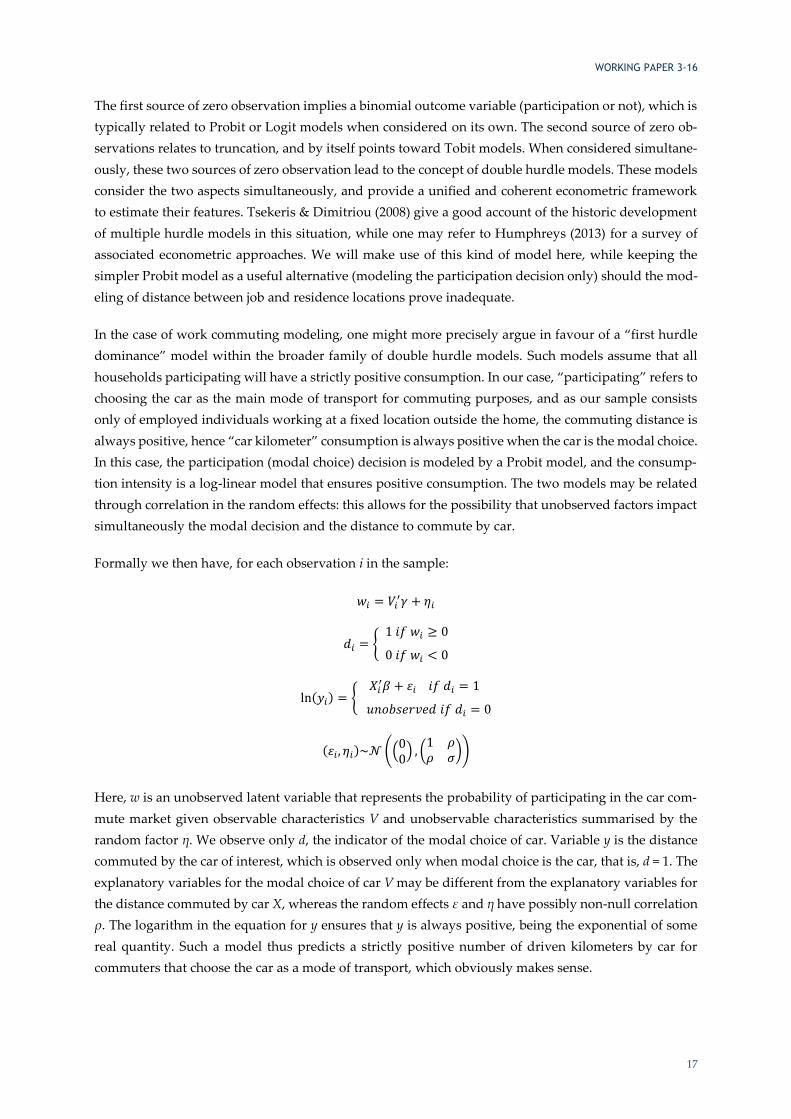
Formally we then have, for each observation i in the sample:

𝑤𝑖 = 𝑉𝑖′𝛾 + 𝜂𝑖

𝑑𝑖 = { 1 𝑖𝑓 𝑤𝑖 ≥ 0

0 𝑖𝑓 𝑤𝑖 < 0

ln(𝑦𝑖) = {𝑋𝑖

′𝛽 + 𝜀𝑖 𝑖𝑓 𝑑𝑖 = 1

𝑢𝑛𝑜𝑏𝑠𝑒𝑟𝑣𝑒𝑑 𝑖𝑓 𝑑𝑖 = 0

(𝜀𝑖, 𝜂𝑖)~𝒩 ((00

) , (1 𝜌𝜌 𝜎

))

Here, w is an unobserved latent variable that represents the probability of participating in the car com-

mute market given observable characteristics V and unobservable characteristics summarised by the

random factor η. We observe only d, the indicator of the modal choice of car. Variable y is the distance

commuted by the car of interest, which is observed only when modal choice is the car, that is, d = 1. The

explanatory variables for the modal choice of car V may be different from the explanatory variables for

the distance commuted by car X, whereas the random effects ε and η have possibly non-null correlation

ρ. The logarithm in the equation for y ensures that y is always positive, being the exponential of some

real quantity. Such a model thus predicts a strictly positive number of driven kilometers by car for

commuters that choose the car as a mode of transport, which obviously makes sense.

WORKING PAPER 3-16

18

The alternative Probit model is obtained by considering only the first stage of this model, with d as the

response variable, and dropping the second equation in y.

Estimation strategy

We now devote some time to our estimation strategy, given the potential presence of endogeneity. Two

sources of problems can be distinguished. First, “car-lovers” may have the tendency to select jobs grant-

ing company cars, independently of transport related considerations. In this case, company car owners

may on average show a higher propensity to use the car as a main commuting mode than other em-

ployees, even after the specific fiscal treatment of company car is abrogated, hence a typical case of

selection bias. Second, as mentioned above, the direction of the causal relation between the presence of

a company car and the commuting distance is unclear, pointing to a case of simultaneity bias.

To address the first issue, related to modal choice, we enrich the set of covariates in the model and

perform the estimation on propensity score matched samples. We include all variables that may reflect

a potential higher propensity to use a car in the modal equation that is in the V vector. In particular, we

include variables reflecting a rather objective but not necessarily work-related need to use a car (such

as the presence of children or the rural nature of the home district), as well as markers of an idiosyncratic

preference for the car with the presence of more than one car in the household and the value index for

the household cars except the most valuable. We then treat the issue as one of selection on observables,

and trim the sample based on a propensity score matching procedure. This ensures company car owners

are matched against employees in the survey sample with comparable characteristics in terms of both

objective and idiosyncratic preference for cars.

The second issue, regarding the endogeneity of the distance from home to work, is more complex to

address given our data source. Indeed, it would ideally call for a joint modeling of the commuting dis-

tance and company car attribution. We do not, however, have enough labour market information in our

data source to propose a credible model for company car attribution. Basic data such as wages, the size

of firms, detailed type of functions, work experience of employees or sector of activity of the firms are

not available and would be required for such a model.

Rather than making wild guesses, we consider two cases in parallel which correspond to the extreme

cases where one or the other effect dominate. This allows us to propose lower and upper bounds for the

impact of the presence of a company car on the total number of kilometers driven by car for commuting

purposes.

In the first case, when the commuting distance is considered endogenous and the presence of a company

car exogenous, we cannot use the commuting distance in the matching process, as it is influenced by

the treatment variable. But there is no simultaneity bias issue, and the double hurdle model, in its first

hurdle dominance flavor, is adequate. We estimate this model on the sample matched on propensity

scores excluding the commuting distance variable.

In the second case, where the commuting distance is considered exogenous and the presence of a com-

pany car endogenous, we can (and should) use the commuting distance in the propensity score model

WORKING PAPER 3-16

19

to perform the matching. But in this case, the double hurdle model makes no sense, as its second equa-

tion would suffer from an obvious reverse causality issue. Under the hypothesis that the presence of a

company car does not cause a change in commuting distance, there is, however, no need to estimate

this second equation to assess the impact of the abrogation of the fiscal treatment of company cars on

car commuting distances. The Probit model of modal choice is sufficient to estimate this impact, and it

is adjusted on the sample matched on propensity score including the commuting distance.

In table 11 we reflect the results of the propensity scoring model including commuting distance, as it

provides an empirical insight into possible mechanisms at work in the attribution of company cars.

Obviously, this cannot replace a thorough investigation of this aspect, including a proper economic

modeling of the associated labour market agent’s decisions. However, it provides some useful back-

ground for further research in this domain.

Table 11 Estimation results for the propensity scoring model

Estimate t-stat Significance

Intercept -9.68 -4.80 ***

Value index of extra cars in the household 6.02 4.06 ***

More than one car in the household 0.38 2.39 **

Log of commuting distance 0.20 3.33 ***

Log of age 6.44 2.66 ***

Log of age squared -2.33 -2.64 ***

Gender = female -0.97 -6.99 ***

Works in private sector 2.26 13.07 ***

Professional level = low -2.53 -8.65 ***

Professional level = medium -1.13 -7.62 ***

Education level 0.45 5.37 ***

Work = part-time 51-99% 0.75 1.69 *

Work = full-time 1.61 3.95 ***

Region of residence = Flanders -0.11 -0.62

Region of residence = Wallonia -0.67 -3.84 ***

Variable work schedules 0.27 2.22 **

*** denotes significance at level 0.01, ** at level 0.05, * at level 0.10

Only significant variables are reported. Influential factors stemming from work characteristics are the

sector of activity (a job in the private sector gives a much higher chance of being granted a company car

than a job in the public sector), the professional level (which has a positive effect on the propensity to

have a company car), the working hours (full-time jobs have higher chances of granting company cars

than part-time jobs), and a variable work schedule, which has some positive impact on the propensity

score. Personal characteristics of importance are the gender of the worker, with a much lower propen-

sity to have company cars for women, and age with a maximum positive effect on the propensity to

have a company car around 40 years for our quadratic specification. The region of residence has a sig-

nificant influence, with Walloon workers showing a lower propensity to have a company car than Flem-

ish and Brussels workers. The variable “more than one car in the household” has a positive impact on

the propensity to have a company car. The variable “value index of the cars in the household except the

WORKING PAPER 3-16

20

highest valued” has a less significant but still positive impact. Thus our markers of idiosyncratic pref-

erence for the car indeed show a positive impact on the propensity score. Last but not least, the com-

muting distance also shows a significantly positive influence on the propensity score. Castaigne et al.

(2010) make similar observations regarding the attribution of company cars, based on an ad-hoc survey.

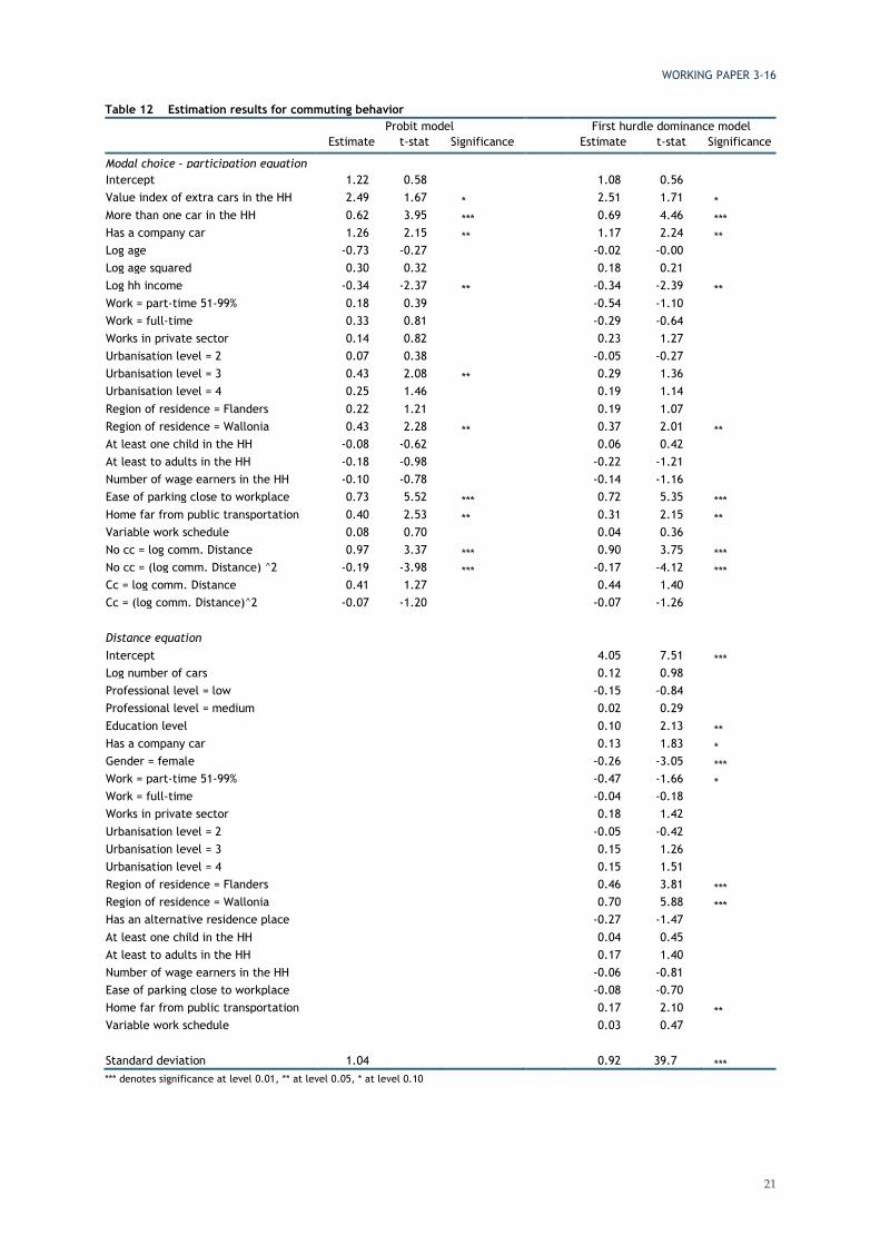
Table 12 provides the estimation result for the two most useful models related to our two alternatives

regarding the causality relation between commuting distance and the presence of a company car: the

Probit model fitted to the sample matched on propensity scores including the commuting distance, and

the first hurdle dominance model fitted to the sample matched on propensity scores excluding the com-

muting distance.

WORKING PAPER 3-16

21

Table 12 Estimation results for commuting behavior

Probit model First hurdle dominance model

Estimate t-stat Significance Estimate t-stat Significance

Modal choice – participation equation

Intercept 1.22 0.58 1.08 0.56 Value index of extra cars in the HH 2.49 1.67 * 2.51 1.71 * More than one car in the HH 0.62 3.95 *** 0.69 4.46 *** Has a company car 1.26 2.15 ** 1.17 2.24 ** Log age -0.73 -0.27 -0.02 -0.00 Log age squared 0.30 0.32 0.18 0.21 Log hh income -0.34 -2.37 ** -0.34 -2.39 ** Work = part-time 51-99% 0.18 0.39 -0.54 -1.10 Work = full-time 0.33 0.81 -0.29 -0.64 Works in private sector 0.14 0.82 0.23 1.27 Urbanisation level = 2 0.07 0.38 -0.05 -0.27 Urbanisation level = 3 0.43 2.08 ** 0.29 1.36 Urbanisation level = 4 0.25 1.46 0.19 1.14 Region of residence = Flanders 0.22 1.21 0.19 1.07 Region of residence = Wallonia 0.43 2.28 ** 0.37 2.01 ** At least one child in the HH -0.08 -0.62 0.06 0.42 At least to adults in the HH -0.18 -0.98 -0.22 -1.21 Number of wage earners in the HH -0.10 -0.78 -0.14 -1.16 Ease of parking close to workplace 0.73 5.52 *** 0.72 5.35 *** Home far from public transportation 0.40 2.53 ** 0.31 2.15 ** Variable work schedule 0.08 0.70 0.04 0.36 No cc = log comm. Distance 0.97 3.37 *** 0.90 3.75 *** No cc = (log comm. Distance) ^2 -0.19 -3.98 *** -0.17 -4.12 *** Cc = log comm. Distance 0.41 1.27 0.44 1.40 Cc = (log comm. Distance)^2 -0.07 -1.20 -0.07 -1.26 Distance equation Intercept 4.05 7.51 *** Log number of cars 0.12 0.98 Professional level = low -0.15 -0.84 Professional level = medium 0.02 0.29 Education level 0.10 2.13 ** Has a company car 0.13 1.83 * Gender = female -0.26 -3.05 *** Work = part-time 51-99% -0.47 -1.66 * Work = full-time -0.04 -0.18 Works in private sector 0.18 1.42 Urbanisation level = 2 -0.05 -0.42 Urbanisation level = 3 0.15 1.26 Urbanisation level = 4 0.15 1.51 Region of residence = Flanders 0.46 3.81 *** Region of residence = Wallonia 0.70 5.88 *** Has an alternative residence place -0.27 -1.47 At least one child in the HH 0.04 0.45 At least to adults in the HH 0.17 1.40 Number of wage earners in the HH -0.06 -0.81 Ease of parking close to workplace -0.08 -0.70 Home far from public transportation 0.17 2.10 ** Variable work schedule 0.03 0.47 Standard deviation 1.04 0.92 39.7 *** *** denotes significance at level 0.01, ** at level 0.05, * at level 0.10

WORKING PAPER 3-16

22

These estimation results identify several characteristics as significant in the determination of kilometers

driven by car for commuting purposes. Based on the coefficient’s sign and magnitude, and focusing on

the statistically significant covariate only, the following summary can be sketched for the Probit model.

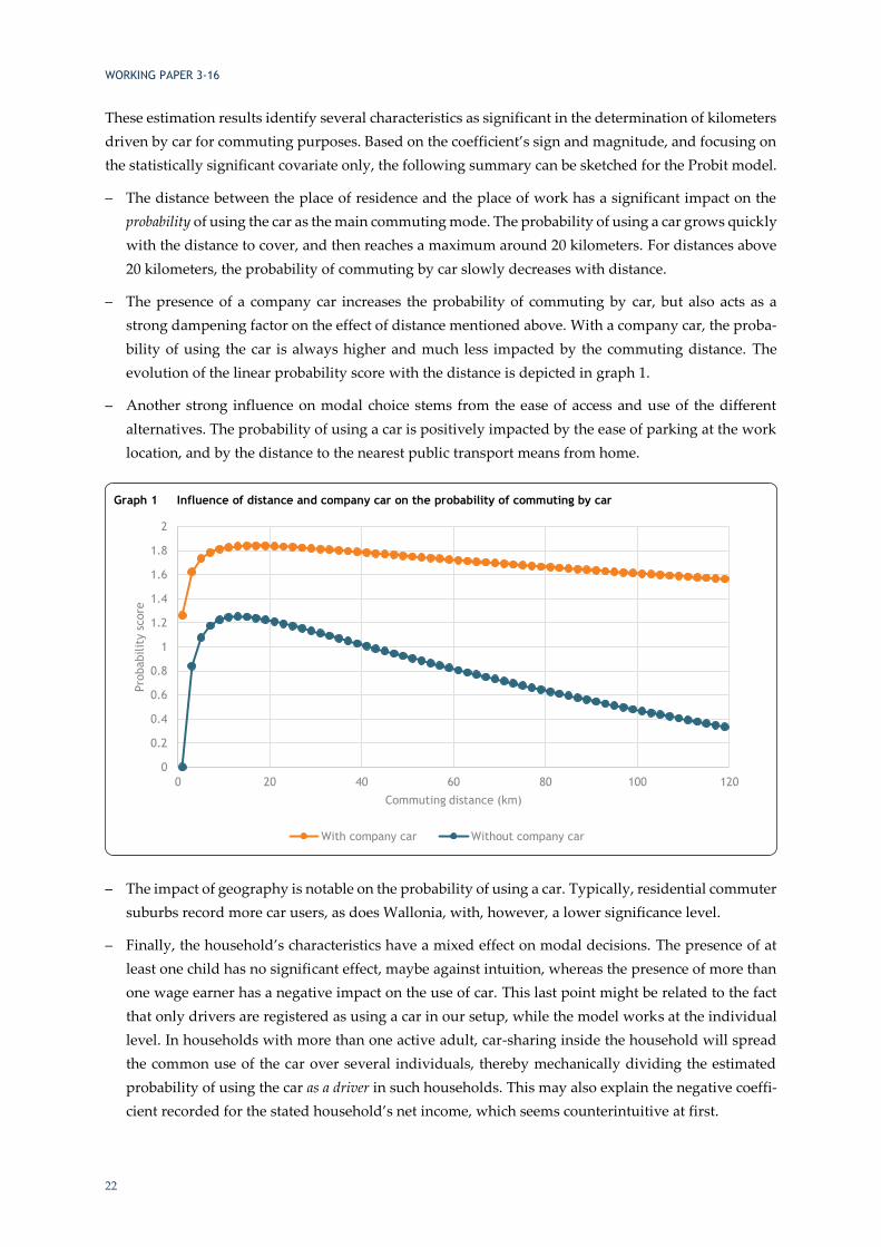
– The distance between the place of residence and the place of work has a significant impact on the

probability of using the car as the main commuting mode. The probability of using a car grows quickly

with the distance to cover, and then reaches a maximum around 20 kilometers. For distances above

20 kilometers, the probability of commuting by car slowly decreases with distance.

– The presence of a company car increases the probability of commuting by car, but also acts as a

strong dampening factor on the effect of distance mentioned above. With a company car, the proba-

bility of using the car is always higher and much less impacted by the commuting distance. The

evolution of the linear probability score with the distance is depicted in graph 1.

– Another strong influence on modal choice stems from the ease of access and use of the different

alternatives. The probability of using a car is positively impacted by the ease of parking at the work

location, and by the distance to the nearest public transport means from home.

– The impact of geography is notable on the probability of using a car. Typically, residential commuter

suburbs record more car users, as does Wallonia, with, however, a lower significance level.

– Finally, the household’s characteristics have a mixed effect on modal decisions. The presence of at

least one child has no significant effect, maybe against intuition, whereas the presence of more than

one wage earner has a negative impact on the use of car. This last point might be related to the fact

that only drivers are registered as using a car in our setup, while the model works at the individual

level. In households with more than one active adult, car-sharing inside the household will spread

the common use of the car over several individuals, thereby mechanically dividing the estimated

probability of using the car as a driver in such households. This may also explain the negative coeffi-

cient recorded for the stated household’s net income, which seems counterintuitive at first.

Graph 1 Influence of distance and company car on the probability of commuting by car

0

0.2

0.4

0.6

0.8

1

1.2

1.4

1.6

1.8

2

0 20 40 60 80 100 120

Pro

babilit

y s

core

Commuting distance (km)

With company car Without company car

WORKING PAPER 3-16

23

When considering the first hurdle dominance model, impacts on the first equation – related to modal

choice – are similar to those recorded for the Probit model above. The only difference is the matching

procedure, which does not include the commuting distance as a matching factor here. This has a limited

impact in terms of results for this first equation. The relevant factors for the distance equation in the first

hurdle dominance model are:

– A limited positive impact of the presence of a company car. The coefficient for this factor is not the

most significant in the model.

– A strong impact of gender, with women showing on average shorter commuting distances, as well

as of the region of residence, with both Wallonia and Flanders logically showing longer commutes

than Brussels, and Wallonia still in significant excess of Flanders in this aspect.

– Other less significant factors with an influence on the total commuting distance are the education

level, with higher-educated workers travelling on average longer commuting distances, as is the case

for private sector workers compared to public sector workers.

Impact analysis

The interpretation of the sign, magnitude and significance of the model parameters provides us with

useful insight regarding the factors’ importance in explaining the variation in car usage for commuting.

But to assess the effect of abrogating the specific fiscal treatment of company cars, we need to compute

the global marginal effect of the related factor in the model. This is somewhat more cumbersome for

such models than for regular linear models, especially due to the presence of significant interactions6

between the presence of a company car and distance variables. We report “average treatment effect on

the treated”, that is the average difference computed for company cars owner were they to trade their

company car for a normal car, or in other words, were the specific fiscal treatment to be abrogated.

Results are for the two models highlighted above and include bootstrapped confidence intervals at 90%,

as well as a decomposition7 of the marginal effect between the part stemming from changes in the prob-

ability of using a car, and that stemming from changes in the commuting distance. Writing y for the

kilometers driven by car and x for the set of explanatory factors, and x:cc the current set of factors for

company car owners vs. x:ncc the counterfactual set of factor with all company cars replaced with nor-

mal cars, we have:

𝑇𝑜𝑡𝑎𝑙 𝑚𝑎𝑟𝑔𝑖𝑛𝑎𝑙 𝑒𝑓𝑓𝑒𝑐𝑡 = 𝔼(𝑦|𝑥 ∶ 𝑐𝑜𝑚𝑝𝑎𝑛𝑦 𝑐𝑎𝑟) − 𝔼(𝑦|𝑥 ∶ 𝑛𝑜 𝑐𝑜𝑚𝑝𝑎𝑛𝑦 𝑐𝑎𝑟)

= ℙ(𝑦 > 0|𝑥: 𝑐𝑐) ∙ 𝔼(𝑦|𝑦 > 0, 𝑥: 𝑐𝑐) − ℙ(𝑦 > 0|𝑥: 𝑛𝑐𝑐) ∙ 𝔼(𝑦|𝑦 > 0, 𝑥: 𝑛𝑐𝑐)

= [ℙ(𝑦 > 0|𝑥: 𝑐𝑐) − ℙ(𝑦 > 0|𝑥: 𝑛𝑐𝑐)] ∙ 𝔼(𝑦|𝑦 > 0, 𝑥: 𝑐𝑐) + ℙ(𝑦 > 0|𝑥: 𝑛𝑐𝑐) ∙ [𝔼(𝑦|𝑦 > 0, 𝑥: 𝑐𝑐) − 𝔼(𝑦|𝑦 > 0, 𝑥: 𝑛𝑐𝑐)]

= [𝑝𝑟𝑜𝑏𝑎𝑏𝑖𝑙𝑖𝑡𝑦 𝑑𝑖𝑓𝑓𝑒𝑟𝑒𝑛𝑐𝑒] ∙ 𝑐𝑢𝑟𝑟𝑒𝑛𝑡 𝑑𝑖𝑠𝑡𝑎𝑛𝑐𝑒 + 𝑐𝑜𝑢𝑛𝑡𝑒𝑟𝑓𝑎𝑐𝑡𝑢𝑎𝑙 𝑝𝑟𝑜𝑏𝑎𝑏𝑖𝑙𝑖𝑡𝑦 ∙ [𝑑𝑖𝑠𝑡𝑎𝑛𝑐𝑒 𝑑𝑖𝑓𝑓𝑒𝑟𝑒𝑛𝑐𝑒]

= 𝑃𝑟𝑜𝑏𝑎𝑏𝑖𝑙𝑖𝑡𝑦 𝑒𝑓𝑓𝑒𝑐𝑡 + 𝐷𝑖𝑠𝑡𝑎𝑛𝑐𝑒 𝑒𝑓𝑓𝑒𝑐𝑡

Results are in kilometers per week for one way commutes, or percentage points for probabilities.

6 Not only do we have two equations involving the company car variable, but this variable also appears in interaction with

other variables. Ad hoc computations are thus required. 7 The principle here is mimicking classical shift-share analysis.

WORKING PAPER 3-16

24

Table 13 Marginal effects of a company car on probability of using a car and on distance travelled for commuting (one way)

Effect First hurdle dominance Probit

Total marginal effect 40.4 (25.9 – 57.8) 29.1 (20.1 – 37.4)

Probability effect 25.3 (19.1 – 31.8) 29.1 (20.1 – 37.4)

Distance effect 15.2 (1.2 – 30.6) 0

Probability difference (pp) 15.9 (12.2– 19.2) 15.9 (11.8 – 19.9)

Distance difference 19.4 (1.5 – 40.0) 0

To provide a unique estimate of the impact of company cars on commuting kilometers driven by car,

we choose to stick to the Probit model. Two reasons, different in nature, guide this choice. First, on an

economic basis, as mentioned above, this model corresponds best to the hypothesis where the commut-

ing distance is exogenous, hence considered fixed independently of the provision or not of a car by the

employer. This hypothesis implies that, were the specific fiscal treatment of company cars to be abro-

gated, employees would not change job or relocate their residence to reduce their commuting distance.

This seems a reasonable hypothesis, at least in the short run, for the Belgian labour and housing markets.

Mobility in the Belgian labour market is not high, and it is even less so in the Belgian housing market.

Then, on a statistical basis, the confidence intervals computed for the “distance effect” based on the

alternative hypothesis and the first hurdle dominance model are very large, and do not rule out a null

effect. It therefore seems more appropriate not to make use of the larger average total effect obtained

under this alternative hypothesis, but to favour the more robust and more cautious effect computed

using the Probit model under the fixed distance hypothesis. We can hence propose an estimated effect

of abrogating the specific fiscal treatment of company cars on kilometers driven for commuting pur-

poses: this would decrease by some 29 km per week the (one way) amount driven by current owners of

company cars on average. This difference would be due solely to a decrease of some 16 percentage

points in the share of car users among current company car owners. Standing at 92.1% in our sample,

this share would thus decrease to 75.1%. This is fully in line with other research for Belgium. This would

remain above the 68.9% share of individuals using the car for commuting purposes while not having a

company car in our sample, 3/4 of the current difference being thus attributed to the presence of a com-

pany car, as opposed to other explanatory factors. The current average usage for company car holders

commuting by car is 152.19 km, and would thus decrease to 123.0 km, as compared to a current average

of 100.11 km for car users without a company car. Here, more than half of the current difference appears

to stem from the presence of a company car. Note that this reduction in average usage is due only to a

decrease of the probability to use the car concentrated on company car holders with the longest com-

mutes should the fiscal regime be abrogated: the individual commuting distances remain fixed. Indeed,

the impact of the fiscal regime applicable to company cars on the total commuting distance is supposed

to be negligible in these figures, as we cannot presently estimate it unambiguously.

We conclude this part with the restatement of its main result: the abrogation of the specific fiscal re-

gime for company cars would, according to our estimates, decrease the number of kilometers driven

for commuting purposes by some 58.2 km per week, or around 2 794 km per year for current company

car users.

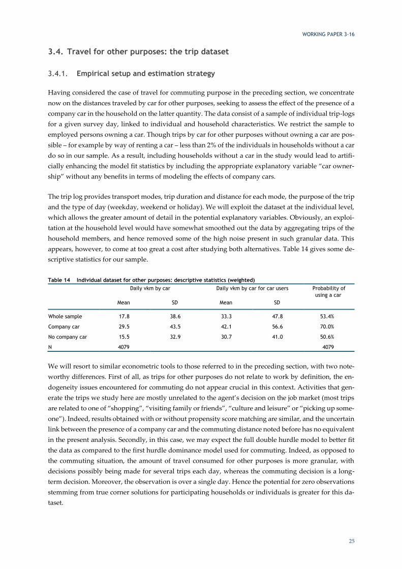
WORKING PAPER 3-16

25

3.4. Travel for other purposes: the trip dataset

Empirical setup and estimation strategy

Having considered the case of travel for commuting purpose in the preceding section, we concentrate

now on the distances traveled by car for other purposes, seeking to assess the effect of the presence of a

company car in the household on the latter quantity. The data consist of a sample of individual trip-logs

for a given survey day, linked to individual and household characteristics. We restrict the sample to

employed persons owning a car. Though trips by car for other purposes without owning a car are pos-

sible – for example by way of renting a car – less than 2% of the individuals in households without a car

do so in our sample. As a result, including households without a car in the study would lead to artifi-

cially enhancing the model fit statistics by including the appropriate explanatory variable “car owner-

ship” without any benefits in terms of modeling the effects of company cars.

The trip log provides transport modes, trip duration and distance for each mode, the purpose of the trip

and the type of day (weekday, weekend or holiday). We will exploit the dataset at the individual level,

which allows the greater amount of detail in the potential explanatory variables. Obviously, an exploi-

tation at the household level would have somewhat smoothed out the data by aggregating trips of the

household members, and hence removed some of the high noise present in such granular data. This

appears, however, to come at too great a cost after studying both alternatives. Table 14 gives some de-

scriptive statistics for our sample.

Table 14 Individual dataset for other purposes: descriptive statistics (weighted)

Daily vkm by car Daily vkm by car for car users Probability of

using a car

Mean SD Mean SD

Whole sample 17.8 38.6 33.3 47.8 53.4%

Company car 29.5 43.5 42.1 56.6 70.0%

No company car 15.5 32.9 30.7 41.0 50.6%

N 4079 4079

We will resort to similar econometric tools to those referred to in the preceding section, with two note-

worthy differences. First of all, as trips for other purposes do not relate to work by definition, the en-

dogeneity issues encountered for commuting do not appear crucial in this context. Activities that gen-

erate the trips we study here are mostly unrelated to the agent’s decision on the job market (most trips

are related to one of “shopping”, “visiting family or friends”, “culture and leisure” or “picking up some-

one”). Indeed, results obtained with or without propensity score matching are similar, and the uncertain

link between the presence of a company car and the commuting distance noted before has no equivalent

in the present analysis. Secondly, in this case, we may expect the full double hurdle model to better fit

the data as compared to the first hurdle dominance model used for commuting. Indeed, as opposed to

the commuting situation, the amount of travel consumed for other purposes is more granular, with

decisions possibly being made for several trips each day, whereas the commuting decision is a long-

term decision. Moreover, the observation is over a single day. Hence the potential for zero observations

stemming from true corner solutions for participating households or individuals is greater for this da-

taset.

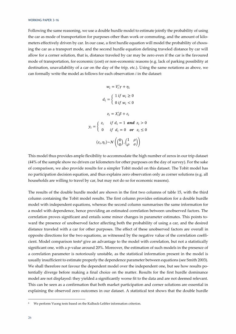
WORKING PAPER 3-16

26

Following the same reasoning, we use a double hurdle model to estimate jointly the probability of using

the car as mode of transportation for purposes other than work or commuting, and the amount of kilo-

meters effectively driven by car. In our case, a first hurdle equation will model the probability of choos-

ing the car as a transport mode, and the second hurdle equation defining traveled distance by car will

allow for a corner solution, that is, distance traveled by car may be zero even if the car is the favoured

mode of transportation, for economic (cost) or non-economic reasons (e.g. lack of parking possibility at

destination, unavailability of a car on the day of the trip, etc.). Using the same notations as above, we

can formally write the model as follows for each observation i in the dataset:

𝑤𝑖 = 𝑉𝑖′𝛾 + 𝜂𝑖

𝑑𝑖 = { 1 𝑖𝑓 𝑤𝑖 ≥ 0

0 𝑖𝑓 𝑤𝑖 < 0

𝑧𝑖 = 𝑋𝑖′𝛽 + 𝜀𝑖

𝑦𝑖 = { 𝑧𝑖 𝑖𝑓 𝑑𝑖 = 1 𝒂𝒏𝒅 𝑧𝑖 > 0

0 𝑖𝑓 𝑑𝑖 = 0 𝒐𝒓 𝑧𝑖 ≤ 0

(𝜀𝑖, 𝜂𝑖)~𝒩 ((00

) , (1 𝜌𝜌 𝜎

))

This model thus provides ample flexibility to accommodate the high number of zeros in our trip dataset

(44% of the sample show no driven car kilometers for other purposes on the day of survey). For the sake

of comparison, we also provide results for a simpler Tobit model on this dataset. The Tobit model has

no participation decision equation, and thus explains zero observation only as corner solutions (e.g. all

households are willing to travel by car, but may not do so for economic reasons).

The results of the double hurdle model are shown in the first two columns of table 15, with the third

column containing the Tobit model results. The first column provides estimation for a double hurdle

model with independent equations, whereas the second column summarises the same information for

a model with dependence, hence providing an estimated correlation between unobserved factors. The

correlation proves significant and entails some minor changes in parameter estimates. This points to-

ward the presence of unobserved factor affecting both the probability of using a car, and the desired

distance traveled with a car for other purposes. The effect of these unobserved factors are overall in

opposite directions for the two equations, as witnessed by the negative value of the correlation coeffi-

cient. Model comparison tests8 give an advantage to the model with correlation, but not a statistically

significant one, with a p-value around 20%. Moreover, the estimation of such models in the presence of

a correlation parameter is notoriously unstable, as the statistical information present in the model is

usually insufficient to estimate properly the dependence parameter between equations (see Smith 2003).

We shall therefore not favour the dependent model over the independent one, but see how results po-

tentially diverge before making a final choice on the matter. Results for the first hurdle dominance

model are not displayed: they yielded a significantly worse fit to the data and are not deemed relevant.

This can be seen as a confirmation that both market participation and corner solutions are essential in

explaining the observed zero outcomes in our dataset. A statistical test shows that the double hurdle

8 We perform Vuong tests based on the Kulback-Leibler information criterion.

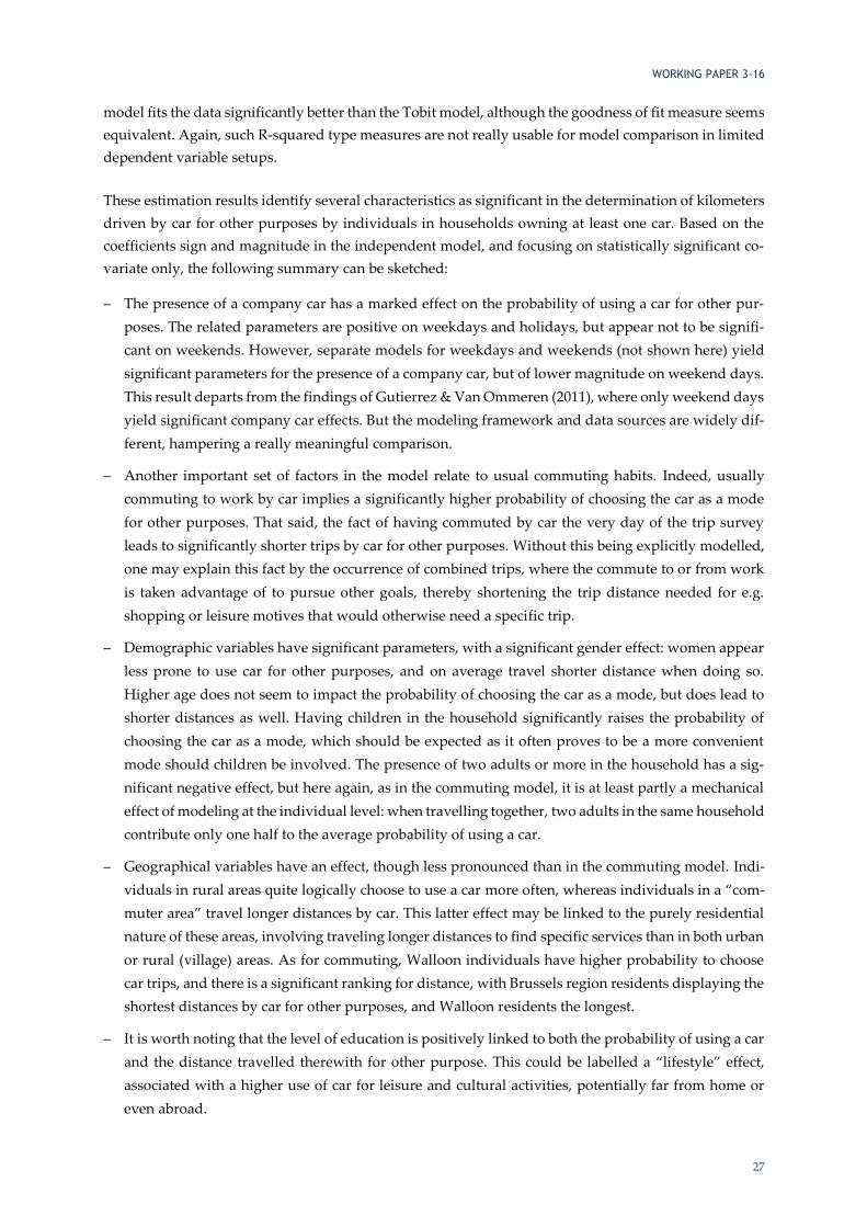
WORKING PAPER 3-16

27

model fits the data significantly better than the Tobit model, although the goodness of fit measure seems

equivalent. Again, such R-squared type measures are not really usable for model comparison in limited

dependent variable setups.

These estimation results identify several characteristics as significant in the determination of kilometers

driven by car for other purposes by individuals in households owning at least one car. Based on the

coefficients sign and magnitude in the independent model, and focusing on statistically significant co-

variate only, the following summary can be sketched:

– The presence of a company car has a marked effect on the probability of using a car for other pur-

poses. The related parameters are positive on weekdays and holidays, but appear not to be signifi-

cant on weekends. However, separate models for weekdays and weekends (not shown here) yield

significant parameters for the presence of a company car, but of lower magnitude on weekend days.

This result departs from the findings of Gutierrez & Van Ommeren (2011), where only weekend days

yield significant company car effects. But the modeling framework and data sources are widely dif-

ferent, hampering a really meaningful comparison.

– Another important set of factors in the model relate to usual commuting habits. Indeed, usually

commuting to work by car implies a significantly higher probability of choosing the car as a mode

for other purposes. That said, the fact of having commuted by car the very day of the trip survey

leads to significantly shorter trips by car for other purposes. Without this being explicitly modelled,

one may explain this fact by the occurrence of combined trips, where the commute to or from work

is taken advantage of to pursue other goals, thereby shortening the trip distance needed for e.g.

shopping or leisure motives that would otherwise need a specific trip.

– Demographic variables have significant parameters, with a significant gender effect: women appear

less prone to use car for other purposes, and on average travel shorter distance when doing so.

Higher age does not seem to impact the probability of choosing the car as a mode, but does lead to

shorter distances as well. Having children in the household significantly raises the probability of

choosing the car as a mode, which should be expected as it often proves to be a more convenient

mode should children be involved. The presence of two adults or more in the household has a sig-

nificant negative effect, but here again, as in the commuting model, it is at least partly a mechanical

effect of modeling at the individual level: when travelling together, two adults in the same household

contribute only one half to the average probability of using a car.

– Geographical variables have an effect, though less pronounced than in the commuting model. Indi-

viduals in rural areas quite logically choose to use a car more often, whereas individuals in a “com-

muter area” travel longer distances by car. This latter effect may be linked to the purely residential

nature of these areas, involving traveling longer distances to find specific services than in both urban

or rural (village) areas. As for commuting, Walloon individuals have higher probability to choose

car trips, and there is a significant ranking for distance, with Brussels region residents displaying the

shortest distances by car for other purposes, and Walloon residents the longest.

– It is worth noting that the level of education is positively linked to both the probability of using a car

and the distance travelled therewith for other purpose. This could be labelled a “lifestyle” effect,

associated with a higher use of car for leisure and cultural activities, potentially far from home or

even abroad.

WORKING PAPER 3-16

28

Table 15 Model estimates: driven kilometres for other purposes

Independent model Dependent model Tobit model

Estimate t-stat Estimate t-stat Estimate t-stat

Participation equation

Intercept -0.26 -0.52 -0.29 -0.59

Day type = weekend 0.09 1.28 0.11 1.79 *

Day type = weekday during holidays 0.18 3.14 *** 0.17 3.36 ***

Used the car to commute that day -0.30 -5.69 *** -0.31 -5.99 ***

Uses the car to commute usually 0.76 13.68 *** 0.77 13.95 ***

Has a company car 0.43 5.00 *** 0.44 5.30 ***

Log income -0.09 -1.62 -0.08 -1.45

Log age 0.04 0.50 0.04 0.51

Gender = female -0.12 -2.72 *** -0.13 -2.88 ***

Urbanisation = 2 -0.03 -0.51 -0.03 -0.39

Urbanisation = 3 0.02 0.29 0.03 0.38

Urbanisation = 4 0.10 1.68 * 0.12 1.94 *

Region = Flanders 0.10 1.33 0.08 0.99

Region = Wallonia 0.26 3.61 *** 0.25 3.51 ***

Child in the household 0.18 3.77 *** 0.13 3.03 ***

Two adults in the household -0.28 -4.57 *** -0.23 -4.23 ***

Education level 0.14 4.67 *** 0.13 4.49 ***

House ownership status = tenant -0.13 -2.15 ** -0.14 -2.35 **

House ownership status = other -0.08 -0.43 -0.04 -0.20

Weekend & has company car -0.56 -3.05 *** -0.43 -2.66 ***

Weekday during holidays & has company

car

0.00 0.00 -0.07 -0.53

Demand equation

Intercept 3.74 6.16 *** 4.57 6.72 *** 0.49 0.41

Used the car to commute that day -0.45 -9.05 *** -0.24 -3.90 *** -0.83 -7.40 ***

Uses the car to commute usually 0.1 1.55 -0.38 -3.84 *** 1.73 14.04 ***

Has a company car 0.25 3.53 *** 0.05 0.57 1.13 6.14 ***

Log income 0.05 0.85 0.12 1.97 ** -0.17 -1.30

Log age -0.42 -4.23 *** -0.47 -4.20 *** -0.18 -0.97

Gender: female -0.19 -3.74 *** -0.14 -2.47 ** -0.39 -4.01 ***

Child in the household 0.39 3.66 ***

Two adults in the household -0.62 -4.68 ***

Urbanisation = 2 -0.04 -0.52 -0.02 -0.21 -0.08 -0.50

Urbanisation = 3 0.19 2.34 ** 0.18 1.90 * 0.18 1.16

Urbanisation = 4 0.06 0.98 0.01 0.09 0.27 2.07 **

Region = Flanders 0.25 2.80 *** 0.18 1.82 * 0.40 2.35 **

Region = Wallonia 0.43 5.11 *** 0.28 2.92 *** 0.84 5.31 ***

Education level 0.07 1.98 ** -0.01 -0.24 0.28 4.28 ***

House ownership status = 0.15 2.28 ** 0.23 2.98 *** -0.19 -1.47

House ownership status = other -0.15 -0.71 -0.10 -0.43 -0.23 -0.59

Day type = weekend 0.24 1.62

Day type = weekday during holidays 0.46 3.63 ***

Weekend & has company car -1.27 -3.20 ***

Weekday during holidays & has company

car

-0.32 -1.08

Correlation between equations -0.75 -11.80 ***

N obs used 3791 3791 3791

R2 0.14 0.14 0.13

WORKING PAPER 3-16

29

Impact analysis

The interpretation of the sign, magnitude and significance of the model parameters provides us with

useful insight regarding the factors’ importance in explaining the variation in car usage for other pur-

poses. Here again, to assess the effect of removing the specific fiscal treatment of company cars, we need

to compute the global marginal effect of the related factor in the model. We report the counterfactual

distance reduction (the average difference computed for company cars owner were they to give up their

company car) for the three models considered in table 16, as well as the bootstrapped confidence inter-

val for a 90% confidence level.

Table 16 Marginal counterfactual effect of the presence of a company car on kilometres driven for other purposes

Model Independent Dependent Tobit

Total effect 6.7 (4.2 – 8.7) 13.3 (6.5 – 23.8) 7.9 (5.2 – 10.1)

Probability effect 3.3 (2.1 – 4.4) 9.7 (3.8 – 17.3) 2.3 (1.4 – 3.0)

Distance effect 3.4 (1.7 – 5.3) 3.7 (-4.3 – 8.9) 5.6 (3.7 – 7.2)

Probability difference (pp) 12.5 (8.5 – 16.2) 12.4 (8.4 – 15.9) 10.9 (7.8 – 14.0)

Distance difference 5.9 (3.0 – 9.2) 6.4 (-8.6 – 15.5) 8.2 (5.4 – 10.4)

The rather unstable estimates produced by the double hurdle model with dependence are striking, read-

ing this table9. Confidence intervals are very large, and the distance effect cannot be qualified as signif-

icant given the variability of estimates, even if on average it appears higher than for the independent

model. Therefore, we shall focus on the independent model on the sequel. As in the previous section,

but with much less emphasis, the Tobit model tends to underestimate the probability effect, despite

having relatively larger parameter estimates, which lead to an important estimated distance effect.

Again, the Tobit model is statistically dominated by the independent model, hence the effects computed

based on the latter are to be favoured.

On the basis of the independent model, we can hence propose an estimated effect of abrogating the

specific fiscal treatment of company cars on kilometers driven for other purposes: this would decrease

the amount driven by current owners of company cars on average by some 6.7 km per day. This differ-

ence would be due to, on the one hand, to a decrease of some 12.5 percentage points in the share of car

users among current company car owners. Standing at 70.0% in our sample, this share would thus de-

crease to 57.5%. This would remain above the 50.6% share of individuals using the car for other pur-

poses while not having a company car in our sample, some 65% of the current difference being thus

attributed to the presence of a company car, as opposed to other explanatory factors. On the other hand,

the total driven distance for other purposes by individuals choosing to travel by car would decrease as

well for company car users, leading to a decrease of some 5.9 km in the average daily car usage for

current company car owners using their car for other purposes. The current usage is 56.6 km, and would

thus decrease to 50.7 km, as compared to a current average of 41.0 km for car users without a company

car. Here, a little more than one third of the current difference in distance appears to stem from the

presence of a company car.

9 One typically witnesses a very high variability of the correlation parameter on the bootstrap subsamples, which leads to a

high volatility of distance effects.

WORKING PAPER 3-16

30

We conclude this part with the restatement of its main result: the abrogation of the specific fiscal re-

gime for company cars would, according to our estimates, decrease the number of kilometers driven

for other purposes by some 6.7 km per day or around 2 445km per year for current company car users.

This translates to 11.8 km per day and 4 304 km per year for one household, based on the average

number of adults per household in our sample. Given an average distance-weighted occupation of

1.4 per vehicle, this translates into 8.2 vehicle km per day, or 2 993 km per year.

Aggregating the results from the models for commuting and for other purposes, we can conclude that

the abrogation of the specific fiscal regime for company cars would, according to our estimates, de-

crease the number of kilometers driven for purposes other than work by some 5 787 km per year for

households with a company car. This is indeed less than the 12 077 km grossly estimated reduction

based on the total driven distance provided by our first model, this latter quantity including kilome-

ters driven for work-related purposes and the impact of selection effects. The discussions related to

the different models above also provide support for the conservativeness of our estimate. Results

obtained by other authors for Belgium are more pronounced, with Castaigne et al. (2010) reporting a

partial effect around 9 200km per year for the presence of a company car in a multiple linear regres-

sion model of car usage based on an ad-hoc survey, but without specific treatment of selection bias.

WORKING PAPER 3-16

31

4. Estimating welfare effects

In the previous section, we have estimated the demand effects of the current company car regime. In

this section, we translate these demand effects into welfare losses to society as a whole. As argued in

section 2, total welfare changes ∆𝑊 can be understood as the sum of changes in consumer surplus ∆𝐶𝑆

and changes in external costs ∆𝐸𝐶.

∆𝑊 = ∆𝐶𝑆 + ∆𝐸𝐶 =1

2∙

∆𝑝𝑝⁄ ∆𝑥 + ∆𝑥(𝑀𝐸𝐸𝐶 + 𝑀𝐸𝐶𝐶)

In this formula, ∆𝑝

𝑝⁄ is the relative price change due to the tax subsidy, ∆𝑥 is the induced demand effect

(in terms of kilometres driven, and car value). 𝑀𝐸𝐸𝐶 and 𝑀𝐸𝐶𝐶 are marginal external environmental

costs and marginal external congestion costs of extra kilometres driven, respectively.

Following formula x, the relative price change is:

∆𝑝𝑝⁄ =

(𝑝 − (𝑝 − 𝐻)𝜏 − 𝑝)𝑝⁄ = −(1 − 𝐻

𝑝⁄ )𝜏

We therefore simply need an estimate of the marginal tax rate 𝜏 facing company car users, and the im-

puted value for tax purposes of the benefit as a percentage of the price. We follow Harding (2014) in

assuming that the relevant marginal tax rate is 61%, which is the all-inclusive rate comprising of per-

sonal income taxes and employee social security contributions, for a high – income earner. For kilome-

tres driven, the value of 𝐻 𝑝⁄ is 0, since the fuel card is exempt of taxation. For the car itself, it is 55%

(Harding, 2014).

The tax subsidy in relative terms is therefore 61% for kilometres driven, and 27.45% for the car.

The central demand effects ∆𝑥 are:

– For the value of the most expensive car in the household: an increase of 62%

– For weekly commuting kilometres: 58.2 vkm per week

– For leisure travel: 8.2 km per day

To arrive at yearly values, we assume people work 48 weeks per year. The average number of company

cars is about 383 400, based on the simulation based on tax return data by the finance ministry for 2011.

Finally, we need additional data relating to prices of a car and of kilometres driven, as well as marginal

external costs.

In order to calculate the components of ∆𝐶𝑆 , the demand effects must be monetarized. For vehicle km

driven, we dispose of data of tax inclusive variable costs per vkm driven. For the year 2012, it is about

0.14 euro per kilometre according to the PLANET database.

For the annual car expenditure, we assume a value of 5 800 per annum. (Harding, 2014) This includes

the depreciation rate, interest and insurance, registration and annual circulation taxes as a percentage

of the car purchase value. Since we don’t directly measure the impact of the company car regime on the

WORKING PAPER 3-16

32

value of a car, but only on the number of CC’s owned by a household, we need a relationship between

engine size and car prices. On the basis of www.vroom.be, an online portal for car manufacturers, we

are able to estimate such a link. As graph 2 shows, there is indeed a close relationship, with car price

increasing by 1.3% with each 1% increase in engine size.

Engine size is clearly not the only factor influencing car prices. Within each engine size class consumers

have access to a range of options and car types that also determine the price of the vehicle. It can be

safely assumed that company car users opt not only for bigger cars, but also choose more expensive

models regardless of engine size. Our calculation of the welfare costs due to more expensive cars based

on the link with engine size alone is therefore likely to be underestimated.

In order to value the external costs of vehicle kilometres driven, we use marginal external cost data from

PLANET database. For environmental costs, we assume about 1.4 cents per vkm. This is as an average

over the whole car park, which may be an underestimate since company cars are more likely to be diesel

cars. On the other hand, they are also relatively newer vehicles which are on average cleaner. Moreover,

for this calculation we assume marginal environmental costs do not change as a result of the policy,

even though the increase in engine size reported in table 8 suggest this may be the case.

For time costs, we distinguish between motives. For commuting, the value is 44 cents, while for other

motives, it is 14 cents per vkm. This is due to the fact that most commuting takes place during the peak

period, as opposed to leisure trips.

Table 17 shows the result of the welfare calculation by car and for the economy as a whole, putting all

the pieces together. Note that external congestion costs are a multiple of the ordinary distortions of

Graph 2 Relation between engine size and car value

8.2

8.7

9.2

9.7

10.2

10.7

11.2

11.7

12.2

12.7

6.5 7 7.5 8 8.5 9

Log s

ale

pri

ce

Log engine size

http://www.vroom.be/

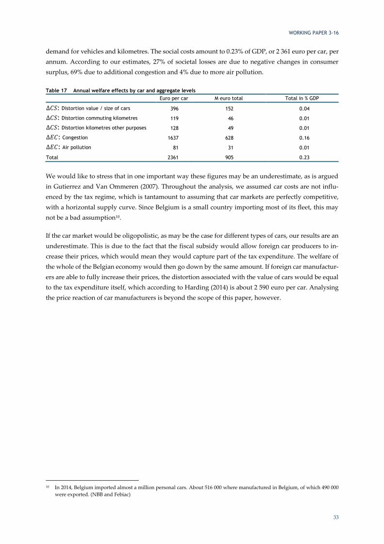
WORKING PAPER 3-16

33

demand for vehicles and kilometres. The social costs amount to 0.23% of GDP, or 2 361 euro per car, per

annum. According to our estimates, 27% of societal losses are due to negative changes in consumer

surplus, 69% due to additional congestion and 4% due to more air pollution.

Table 17 Annual welfare effects by car and aggregate levels

Euro per car M euro total Total in % GDP

∆𝐶𝑆: Distortion value / size of cars 396 152 0.04

∆𝐶𝑆: Distortion commuting kilometres 119 46 0.01

∆𝐶𝑆: Distortion kilometres other purposes 128 49 0.01

∆𝐸𝐶: Congestion 1637 628 0.16

∆𝐸𝐶: Air pollution 81 31 0.01

Total 2361 905 0.23

We would like to stress that in one important way these figures may be an underestimate, as is argued

in Gutierrez and Van Ommeren (2007). Throughout the analysis, we assumed car costs are not influ-

enced by the tax regime, which is tantamount to assuming that car markets are perfectly competitive,

with a horizontal supply curve. Since Belgium is a small country importing most of its fleet, this may

not be a bad assumption10.

If the car market would be oligopolistic, as may be the case for different types of cars, our results are an

underestimate. This is due to the fact that the fiscal subsidy would allow foreign car producers to in-

crease their prices, which would mean they would capture part of the tax expenditure. The welfare of

the whole of the Belgian economy would then go down by the same amount. If foreign car manufactur-

ers are able to fully increase their prices, the distortion associated with the value of cars would be equal

to the tax expenditure itself, which according to Harding (2014) is about 2 590 euro per car. Analysing

the price reaction of car manufacturers is beyond the scope of this paper, however.

10 In 2014, Belgium imported almost a million personal cars. About 516 000 where manufactured in Belgium, of which 490 000

were exported. (NBB and Febiac)

WORKING PAPER 3-16

34

5. Discussion

This paper has attempted to estimate the impact of having a company car on car size, value and the

number of vkm kilometres driven for private trips. The effects that have been found are quite large,

though not extreme as compared to other similar studies in Belgium and the Netherlands. The value of

the first car in the household increases by 62%, while the number of weekly kilometres by car for com-

muting rises by 58.2 km. Daily car vkm for other (private) purposes rises by 8.2 km per day, per house-

hold.

This excessive use of the car translates into large annual welfare losses. Per car, these are estimated at

2 361 euro per annum, most of which are due to external congestion costs and excessive consumption

of car units and kilometres driven. 81 euro per car is lost due to additional emissions of greenhouse

gases and air pollutants. Total losses to society amount to 0.23% of GDP.

It should be noted that the estimates in this paper only give effects of a wholesale abolishing of the

current company car regime. In reality, policy changes are more likely to be piecemeal, and may be

accompanied by compensatory measures, such as lowering labour income taxes or increasing subsidies

on commuting by other modes. The results in this paper could be used to calibrate a simulation model

that analyses the effects of more realistic policy packages.

It should also be noted that the welfare effects on this model are of a partial equilibrium nature. When

interactions with other markets are significant, conclusions may change. For example, if less car use

leads to more intensive use of public transport, one should take into account the second order effects

from such a shift on public finances and the environment as well. This may be done by embedding this

model in a general equilibrium model.

Some of the results in this paper point to further research. For example, we noted that the effect of the

company car on car use for other purposes than commuting was largest during the weekdays. This may

suggest that people build trip chains: commuting is combined with other trip purposes such as shop-

ping or driving children to school. If this is the case, policies that influence commuting may have spill-

overs onto other markets as well.

The link between the presence of a company car and the observed distance between place of residence

and place of work is another topic for further research. In this paper, while we acknowledge the exist-

ence of such a link, the home-work distance has been considered exogenous, which at best is a hypoth-

esis valid only in the short term. More generally, developing a more sophisticated labour market model

would allow this and other issues, such as the mechanism for company car attribution, to be addressed

more robustly. Relying on such a model will make endogeneity and selection issues more transparent

and provide workarounds, and therefore prepare the ground for more precise estimates.

WORKING PAPER 3-16

35

6. Bibliography

Gutierrez – i – Puigarnau, E. and J. Van Ommeren (2007), ‘Welfare Effects of Distortionary Car Taxation’,

Tinbergen Discussion Paper, 2007-060/3.

Gutierrez – i – Puigarnau, E. and J. Van Ommeren (2011), ‘Welfare Effects of Distortionary Fringe Benefit

Taxation: The Case of Employer-Provided Cars’, International Economic Review, 52(4), pp. 1105-1122.

Harding, M. (2014), ‘Personal Income Tax Treatment of Company Cars and Commuting Expenses’, OECD

Taxation Working Papers, No. 20.

De Borger B. and I. Mayeres (2004), ‘Taxation of Car Ownership and Public Transport: Insight Derived from

a Discrete Numerical Optimization Model’, KUL-ETE, WP 2004-13.

De Borger B. and B. Wuyts (2011), ‘The tax treatment of company cars, commuting and optimal congestion

taxes’, Transportation Research B: Methodological, Elsevier, vol 45(10), pp. 1527-1544.

De Witte, A. and Macharis, C. (2010), ‘Commuting to Brussels: how attractive is ‘free’ public transport’, Brus-

sels Studies 37.

Cornelis, E., K. Declercq, L. Hollaert, P. Huynen, D. Janssens, & F. Walle (2011a), ‘Premiers résultats de

l'enquête nationale de mobilité 2010 : BELDAM’, Namur: FUNDP. Namur center for complex system.

Cornelis, E., Macharis, C., Toint, P. and G. Wets (2011b), ‘Professional mobility and car ownership: final

report’, Belspo.

Deaton, A. (1986), ‘Demand Analysis’, In Handbook of Econometrics. Amsterdam and New York: New-

Holland.

Eakins, J. (2016), ‘An Application of the Double Hurdle Model to Petrol and Diesel Household Expend-

itures in Ireland’, to appear in Transport Policy, April 2016, 47, pp. 84-93.

Humphreys, B.R. (2013), ‘Dealing With Zeros in Economic Data’, manuscript, University of Alberta.

Macharis, C and A. De Witte (2012), ‘The typical company car user does not exist: the case of the Flemish

company car drivers.’, Transport Policy 24(11), pp. 91-98.

Pfeffermann, D. (1993), ‘The Role of Sampling Weights When Modeling Survey Data’, International Sta-

tistical.

Shiftan, Y., Albert, G. and T. Keinan, (2012), “The Impact of Company Car Taxation on Travel Behavior”,

Transport Policy, 19, pp. 139-146.

Smith, M.D. (2003), ‘On Dependency in Double Hurdle Models’, Statistical Papers, 44(4), pp. 581-595

Ramaekers, K., Wets, G., De Witte, A., Macharis, C., Cornelis, E., Castaigne, M and Pauly, X. (2010), ‘The

impact of company cars on travel behaviour”, 12th WCTR, 2010.

Tobin, J. (1958), ‘Estimation of Relationships for Limited Dependent Variables’, Econometrica, 26(1), pp. 24-36

Tsekeris, T. & Dimitriou, L. (2008), ‘Modeling Participation and Consumption in the Greek Interurban

Public Transportation Market’ Journal of Public Transportation, 11(2), pp. 85-104.

https://cris.cumulus.vub.ac.be/portal/en/persons/cathy-macharis%28819ab358-7db2-4eea-9377-25ba5b153ad3%29.html

https://cris.cumulus.vub.ac.be/portal/en/persons/cathy-macharis%28819ab358-7db2-4eea-9377-25ba5b153ad3%29.html

https://cris.cumulus.vub.ac.be/portal/en/publications/the-typical-company-car-user-does-not-exist-the-case-of-the-flemish-company-car-drivers%28c0840a96-b80e-495b-8150-dd739f7f3371%29.html

https://cris.cumulus.vub.ac.be/portal/en/publications/the-typical-company-car-user-does-not-exist-the-case-of-the-flemish-company-car-drivers%28c0840a96-b80e-495b-8150-dd739f7f3371%29.html

the fiscal treatment of company cars in belgium · working paper 3-16 the fiscal treatment of...

Documents