The Fiscal Cost of Hurricanes: Disaster Aid VersusSocial Insurance

Tatyana Deryugina∗

May 16, 2016

Abstract

Little is known about the fiscal costs of natural disasters, especially regarding social safety

nets that do not specifically target extreme weather events. This paper shows that US hurri-

canes lead to substantial increases in non-disaster government transfers, such as unemployment

insurance and public medical payments, in affected counties in the decade after a hurricane.

The present value of this increase significantly exceeds that of direct disaster aid. This implies,

among other things, that the fiscal costs of natural disasters have been significantly underesti-

mated and that victims in developed countries are better insured against them than previously

thought.

JEL codes: Q54, H84, H53.∗Department of Finance, University of Illinois at Urbana-Champaign. E-mail: deryugin@illinois.edu. This paper

was previously circulated under the title “The Role of Transfer Payments in Mitigating Shocks: Evidence from theImpact of Hurricanes.” I thank Matthew Shapiro and two anonymous referees for helpful comments that significantlyimproved the paper. I am very grateful to Amy Finkelstein and Michael Greenstone for invaluable feedback andguidance. I thank Kathy Baylis, Jeff Brown, Joseph Doyle, Kerry Emanuel, Don Fullerton, Josh Gottlieb, Tal Gross,Jerry Hausman, Daniel Keniston, Patrick Kline, Steven Levitt, Randall Lewis, Anup Malani, Gilbert Metcalf, Er-wann Michel-Kerjan, Nolan Miller, Kevin Murphy, Mariya Pivtoraiko, Jim Poterba, Mar Reguant, Julian Reif, JosephShapiro, and Chad Syverson for useful discussions and feedback. I also thank participants at the NBER Universities’Research Conference, the MIT Public Finance Lunch and Political Economy Breakfast, the University of ChicagoApplied Microeconomics Lunch, and the Harvard Environmental Economics Lunch. A big thanks goes to StephanieSieber for help with spatial data. Jenna Weinstein provided excellent research assistance. Support from the MITEnergy Fellowship and the National Science Foundation is gratefully acknowledged.

1

Economic shocks due to extreme weather are significant and expected to grow in magnitudedue to population movements, ecosystem alteration, and climate change (Board on Natural Dis-asters, 1999; IPCC, 2012, 2013). Consequently, real disaster costs are high and growing fasterthan GDP (Freeman, Keen and Mani, 2003; Bouwer et al., 2007). While much research has beendone on the direct damage inflicted by extreme weather and on the impact of natural disasterson incomes and employment, relatively little attention has been paid to the fiscal cost of the aidresponse, which is often substantial. Less attention still has been paid to the costs borne by so-cial safety net programs, such as traditional unemployment insurance, that do not target disastervictims specifically, but which may be triggered by such events. Transfers from traditional socialsafety nets provide insurance against natural disasters and could be delivering substantial benefitsto victims. At the same time, because the costs of such transfers are not covered by the recipients,moral hazard problems may lead individuals to live in riskier places and take fewer precautionsthan they would with actuarially fair insurance. More generally, measuring the fiscal costs of dis-asters is important for understanding governments’ long-term budgeting needs, for illuminatingthe mechanisms behind disasters’ economic impacts, and for painting a more complete picture ofdisasters’ social costs.

This paper provides the first estimates of the fiscal costs of US hurricanes, taking into accountboth direct costs (i.e., through the disaster aid channel) and indirect costs (i.e., through other socialsafety net programs). Using data that span the years 1969–2012, I estimate changes in governmentnon-disaster transfers received by individuals in US counties in the ten years following a hurricanestrike. I focus on hurricanes that occurred in 1979–2002, which allows me to observe outcomesfor 10 years before and after each hurricane. I employ a differences-in-differences framework,comparing counties that experience hurricanes with those that do not, to estimate how hurricanesaffect transfers that are part of the broader social safety net, such as income maintenance payments,unemployment insurance, and public medical benefits. To provide context for these results and tounderstand the mechanisms that drive them, I also consider changes in other outcomes, includingpopulation, demographics, earnings, and employment.

My results show that considering disaster aid alone substantially understates the fiscal costs ofnatural disasters. Funds provided through official disaster declarations, i.e., disaster aid, average$155-$160 per capita per hurricane during my study period. By contrast, I estimate that in the tenyears following a hurricane an affected county receives extra transfers through non-disaster socialinsurance programs averaging about $780-$1,150 per capita in present value.1 Another measureof transfers available to me includes private insurance payments as a component (referred to as“transfers from businesses to individuals” in my data). These transfers increase temporarily aswell, but they add less than $25 per capita to total transfers, with the majority of the increase

1All monetary amounts have been converted to 2013 dollars using the Consumer Price Index.

2

occurring in the year of the hurricane.Together, the disaster aid and social insurance transfers offset a substantial amount of hurri-

canes’ immediate capital damage, which the Federal Emergency Management Agency (FEMA)estimates to be $700 per capita for major (Category 3 and higher) hurricanes during my studyperiod. I also find that counties are resilient following hurricane strikes: there is no systematic evi-dence of a drop in average earnings, and the employment rate is estimated to be significantly loweronly 5-10 years afterwards. Similarly, population remains unchanged. Overall, the estimates showthat (a) the fiscal impact of hurricanes in the US is much greater once we account for transfersthrough non-disaster social safety nets and (b) disaster aid and social insurance transfers togetheroffset a large share of the damage of a typical US hurricane, implying that victims of such disastersin developed countries are better insured against them than previously thought. However, given theconfidence intervals of the earnings estimates, I cannot rule out that victims experience a net lossof several hundred dollars per capita.

I contribute to two main strands in the literature. The first focuses on the response of localeconomies to shocks, typically focusing on outcomes such as employment, population, and wages(e.g., Blanchard and Katz, 1992; Card, 2001; Cortes, 2008; Autor, Dorn and Hanson, 2013). Withthe exception of Autor et. al. (2013), who study how labor markets in the US are affected by tradecompetition with China, the extant research ignores the fiscal costs of and response to these shocks.I show that the inflow of government funds into a county following a hurricane is substantial, ex-ceeding official disaster aid on average. Thus, such shocks not only cause local economic damagebut also incur a substantial fiscal cost. Moreover, while Autor et. al. (2013) find that transfers madethrough Trade Adjustment Assistance (or TAA, a program specifically aimed at helping workershurt by trade) are two orders of magnitude smaller than transfers from general social safety netprograms in per capita terms, I find that disaster-specific transfers to hurricane-affected countiesare smaller but on the same order of magnitude as non-disaster transfers.

I also contribute to the literature on the economic impacts of natural disasters, which has typi-cally focused on income. Studies in this area typically use GDP or GDP-equivalents as outcomesand thus miss disasters’ impacts on government transfer payments. Consistent with my results,previous researchers have largely found very small or no long-run impacts on income in developedcountries (e.g., Murphy and Strobl, 2010; Strobl, 2011).2 An important exception to this trend isa study by Hsiang and Jina (2014), who find that hurricanes reduce national incomes for at leasttwenty years in both developing and developed countries.

Few studies have examined employment or population in developed countries following naturaldisasters. Consistent with my estimates, Strobl (2011) finds that a US coastal county’s overall

2For a more comprehensive review of the literature, see Cavallo and Noy (2010), Kousky (2012), and Bergeijk andLazzaroni (2015).

3

population is unchanged following a hurricane. Belasen and Polachek (2008) find that county-level employment in Florida is lower for two years following a hurricane. I contribute to thisliterature by considering a much more comprehensive set of outcomes for a large set of disastersover a longer time period. Importantly, I show that ignoring non-disaster transfer flows, as thepreceding literature does, paints an incomplete picture of post-disaster dynamics.

With the exception of Noy and Nualsri (2011), studies of financial flows in the aftermath of adisaster are either theoretical or focused on country-level measures of aid and remittances (Yang,2008; Hochrainer, 2009; Cavallo and Noy, 2010).3 Noy and Nualsri (2011) examine country-level government spending and revenue dynamics following disasters, finding them to be counter-cyclical for developed countries. While I do not consider the cyclicality of transfers or the revenuethat finances them, I am able to distinguish between disaster and non-disaster transfers and comparetheir magnitudes explicitly.

The rest of the paper is organized as follows. Section I provides background information onhurricanes, US federal disaster aid, and the data used for the analysis. Section II describes theempirical strategy. Sections III and IV present and discuss the results, respectively. Section Vconcludes.

I Background and Data

A Hurricane Damage in the United States

Hurricanes that affect the US form in the Atlantic Ocean. Warm humid air over the ocean createsstorms known as “tropical disturbances.” If circulating winds develop, such a disturbance becomesa tropical cyclone. Prevailing winds and currents move the cyclone across the ocean, where itgains or loses strength, depending on conditions. Sometimes a circular area with low internal windspeeds, called the “eye,” develops in the system’s center. Although the entire storm system canspan a few hundred miles, the strongest winds occur on the perimeter of the eye (the “eyewall”).Wind intensity diminishes quickly as one moves away from the eyewall (or the center of the storm,if it has no eye). The outer parts of the hurricane are called “spiral bands.” These are characterizedby heavy rains but typically do not carry hurricane-force winds. When a cyclone encounters land,it loses strength quickly. Thus, counties that are close to the coast bear the brunt of a storm’simpact.

North Atlantic cyclones are classified by maximum 1-minute sustained wind speeds using theSaffir-Simpson Hurricane Scale. A “tropical storm” is a cyclone with wind speeds of 39-73 milesper hour. Cyclones with lower wind speeds are called “tropical depressions.” A cyclone is con-sidered a hurricane if maximum 1-minute sustained wind speeds exceed 74 miles per hour; I use

3For an in-depth conceptual discussion of relevant considerations when designing social safety nets to addressnatural disasters, see Pelham, Clay and Braunholz (2011).

4

this cutoff value throughout. Category 1 and 2 hurricanes are “minor hurricanes,” characterized bymaximum wind speeds of 74-95 and 96-110 mph, respectively. Category 3-5 hurricanes have windspeeds greater than 111 mph and are called “major hurricanes.”

To track where hurricanes hit, I use the Hurricane Data 2nd generation (HURDAT2) datasetfrom the National Hurricane Center.4 It contains the storm center location, wind speed, and atmo-spheric pressure for each North Atlantic cyclone since 1851, in six-hour intervals. I assume thatthe storm path is linear between any two given points and that the wind speed changes smoothly.I supplement these data with the Extended Best Track Dataset, which has estimates of the “max-imum wind speed radius” (MWSR), the distance between a cyclone’s center, and the perimeterof the strongest winds for storms occurring in 1988 and later.5 The MWSR measures the spatialspan of a hurricane’s strongest winds. The MWSRs of earlier hurricanes are not available; I infertheir MWSR based on their maximum wind speeds and pressure.6 I then assume that every countywithin the MWSR is affected. Although the hurricane data span a long time period, annual county-level economic data are available for only 1969–2012. Because my econometric approach uses10 leads and lags and a balanced panel of hurricanes, the storms in my analysis occurred between1979 and 2002.

Between 1979 and 2002, two to eleven North Atlantic hurricanes formed each year, averagingsix per year. Slightly more than one-third of these hurricanes reached major hurricane strength.Approximately one-third of all hurricanes made landfall, and about half of these were major hurri-canes at some point in time. However, many hurricanes lose strength before making landfall. Mysample period includes six years in which no storms made landfall at hurricane strength. Hurri-canes that do make it to land cause widespread wind and flood damage: physical damage fromhurricanes in the US has averaged $4.8 billion per hurricane or $8.1 billion per year between 1970and 2005. If the year that Hurricane Katrina made landfall (2005) is excluded, that figure is $2.4billion per hurricane or $4.0 billion per year.7

US hurricanes are geographically concentrated, and only states close to the Atlantic and Gulf ofMexico coasts have ever experienced cyclones with hurricane-strength winds. Figure 1 shows thedistribution of hurricane hits between 1979 and 2002, with darker areas indicating more hurricanes.In total, 409 counties experienced one or more hurricanes between 1979 and 2002 (282 experiencedonly one).

To gauge the potential economic impact of hurricanes, it is helpful to look more closely at the

4Available from http://www.aoml.noaa.gov/hrd/hurdat/Data_Storm.html. Accessed October2013.

5Available from http://rammb.cira.colostate.edu/research/tropical_cyclones/tc_extended_best_track_dataset/. Accessed February 2014.

6For more details, see Section 2 of the Online Appendix, which can be found at http://deryugina.com/2016-05-16-Deryugina-safety-net-Appendix.pdf.

7Author calculations using data from Nordhaus (2006).

5

damage they cause. To assess hurricane damage, I use estimates of direct damage from HAZUS-MH, a software program published by FEMA to help state, local, and federal government officialsprepare for disasters and to help the private sector estimate risk exposure.8 In addition to simulatinghypothetical damage, HAZUS-MH contains highly detailed engineering-based damage estimatesof past major hurricanes.9 In the Online Appendix, I also consider hurricane damage relative toother extreme weather events, showing that hurricanes are, on average, the most damaging of thecommon meteorological events in my sample (Table A2).

Table 1 shows county-level damage statistics for ten major hurricanes that made landfall inthe United States from 1979 through 2002, including total loss, per capita loss, and the numberof displaced households. Total loss includes estimates of structural damage to buildings, buildingcontent, and inventory loss. Panel A shows the estimated damage in counties that, by my calcu-lations, were within the MWSR and experienced hurricane-strength winds (74 miles per hour ormore). This sample corresponds to the way I identify hurricane-affected counties throughout thepaper. The damage experienced by these counties is substantial: total loss averaged $200 millionor $700 per capita, and about 520 households were displaced.

Panels B and C split up the sample in Panel A into counties that experienced wind speeds of74-111 miles per hour (Panel B) and over 111 miles per hour (Panel C). Because wind’s destruc-tiveness rises non-linearly with speed, I expect the latter counties to suffer more damage. Indeed,counties in Panel B experience lower-than-average damage of $235 per capita while counties withwind speeds of more than 111 miles per hour suffer damage of almost $4,100 per capita.

Finally, Panel D shows the estimated effects of hurricanes on counties that are (a) consideredto be affected in the FEMA simulations but are not within the MWSR and (b) direct neighborsof counties that are within an MWSR. The estimated damage is small: the average loss was only$1.9 million, which is over 100 times smaller than the corresponding estimate in Panel A. Percapita total losses were about 20 times smaller, averaging only $32 per capita. No householdsare estimated to have been displaced, on average. Including all affected neighboring counties inthis summary whether or not they border counties within an MWSR makes the relative damage inMWSR counties even greater. Thus, using the MWSR to identify counties where hurricanes causenon-trivial damage is sensible.

B Federal Disaster Aid

A county can receive specially targeted federal disaster aid if the state’s governor files a request andprovides evidence that the state cannot manage the disaster on its own. The US president makesthe final decision about whether to declare a disaster. If the request is approved, federal money can

8The software is available by request from http://www.fema.gov/hazus#5.9See Online Appendix Table A1 for the list of hurricanes, the estimated damage each caused, and the disaster aid

each received.

6

be used to repair public structures and to make individual and business grants and loans. FEMAalso provides personnel, legal help, counseling, and special unemployment payments for those leftunemployed by a disaster. Although long-term recovery spending is provided in some cases, mostdisaster-specific transfers to individuals occur within six months of a declaration, and most publicinfrastructure spending occurs within two to three years (FEMA, personal communication).

Between 1979 and 2002, the federal government spent $19 billion on hurricane-related dis-aster aid and $67.7 billion on other disasters through formal federal disaster declarations.10 TheNorthridge earthquake in 1994 ($11.1 billion) and the World Trade Center attacks in 2001 ($11.6billion) caused a large fraction of the non-hurricane disaster spending. Excluding these two eventsimplies that hurricane-related spending accounted for nearly half of all disaster aid during thisperiod. Unfortunately, annual county-level data on spending specifically aimed at natural disas-ters is not available, so I cannot incorporate such spending into my main empirical framework.11

However, the available data allow me to approximate the amount of disaster-specific transfers percounty.

Table 2 presents the summary statistics for federal aid related to hurricanes during 1979-2002.Because data on federal disaster aid is on the level of a declaration, which includes multiple coun-ties in a state, I must assume how the money is divided among counties. As I show above, countiesthat fall within an MWSR experience much more damage than their neighbors. Therefore, one nat-ural assumption is that the money is split among only those counties. Another natural assumptionis that the money is divided among the included counties in proportion to the population in eachcounty. A third natural assumption is that the money is divided in proportion to the wind speed. Iapplied all three of these assumptions in the analysis; the results are shown in separate columns inTable 2.

Panel A shows federal disaster aid transfers assuming that only counties that fall within anMWSR and experience hurricane-strength winds are given aid. If I assume that the money is splitequally among all counties, the average per-hurricane amount of aid given to these counties was$15 million per county or about $160 per capita (Columns 1 and 4). Counties that were affected bythe major hurricanes in the HAZUS-MH damage simulations and experienced hurricane-strengthwinds received slightly more on a per capita basis ($185). Of these, counties that experienced wind

10PERI Presidential Disaster Declarations database (Sylves and Racca, 2010). This number includes all declaration-related spending by FEMA, including assistance given for infrastructure repair, individual grants, and mitigationspending. The Small Business Administration also offers subsidized loans to affected individuals and businesses,which are not included here. Spending by state and local governments is also excluded. By law, the state may berequired to contribute to the relief effort, but its share of the total cannot exceed 25%. Thus, accounting for statespending could increase these statistics by up to one-third.

11The Consolidated Federal Funds Report series, which begins in 1983, contains county-level information on disas-ter aid in principle. However, the bulk of disaster-related spending is assigned to state capital county areas rather thancounties actually affected by the disaster, making it unusable for analysis.

7

speeds of 74-111 miles per hour received $155 per capita while those that experienced wind speedsof more than 111 miles per hour received $400 per capita. The estimates are similar if I assumethat the money is split in proportion to wind speed (Columns 3 and 5).

Panel B shows the same statistics assuming that the money is divided among all counties in-cluded in the declaration, not just those falling within an MWSR. Depending on which assumptionabout how the money is split applies, the implied per capita spending for MWSR counties rangesfrom $70 to $100. Hurricane-affected counties in the HAZUS-MH damage simulations receivedslightly more aid, between $105 and $145 per capita. Based on the previous analysis of damageto MWSR counties vis-a-vis their neighbors, it seems most reasonable to assume that the formerreceive all of the aid and that it is allocated between them in proportion to their populations or windspeeds (Columns 4 and 5 in Panel A). This assumption yields estimated disaster transfers of $155-$160 per capita. In the following sections, I use this range as a benchmark to compare disasterrelief spending with non-disaster transfer spending triggered by hurricanes. To compare disasteraid spending to damage estimates, which are only available for hurricanes in the HAZUS-MHsimulations, I use the corresponding estimate of $180-$185 per capita.

It is worth noting that non-profit organizations, such as the Red Cross, may also play an im-portant role in post-disaster dynamics. More broadly, charitable donations represent another po-tentially important transfer. For example, Americans donated an estimated $3.3 billion to helpvictims of Hurricane Katrina, which struck the Gulf Coast in 2005, $1.6 billion after the SouthAsian tsunami of 2004, and $1.4 billion after the 2010 earthquake in Haiti (Charity Nagivator,n.d.). However, because there is no systematic data on charitable donations accruing to a particulararea, I cannot capture the role of charities.

C Economic Data and Control Group

Annual county-level data on population, wages, and government transfer payments come from theRegional Economic Information System (REIS), published by the Bureau of Economic Analysis.Annual county-level population by race and age are from the Surveillance Epidemiology and EndResults (SEER) population database. Finally, data on employment is from the County BusinessPatterns (CBP) database. All three series span the years 1969-2012.12 I define the county employ-ment rate as the ratio of total employment, as reported by CBP, to the number of people aged fifteenand older, as reported by SEER.13 REIS reports wage and salary payments per capita, which I useto measure the average wage. REIS also contains a proxy for private insurance payments: trans-fers from businesses to individuals. This measure consists primarily of net insurance settlementsand personal injury liability payments to non-employees. Thus, any changes in these transfers

12The underlying source of the population data in both REIS and SEER is the US Census Bureau. For details onhow the annual population data are constructed, see the Online Appendix.

13Annual county-level unemployment rates are not available until 1990.

8

following a hurricane are likely to be driven by insurance payouts.14

Finally, REIS provides information on total government transfer flows into each county. Inaddition to analyzing changes in total government transfers, I consider changes in their compo-nents. Total government transfers to individuals include unemployment insurance, income mainte-nance payments (which includes Supplemental Security Income (SSI), family assistance, and foodstamps), retirement and disability insurance benefits, public medical benefits other than Medicare,Medicare, veterans’ benefits, and federal education and training assistance.

To infer the causal effects of hurricanes accurately, one needs to establish a credible counter-factual. A natural starting point is to treat all unaffected counties as potential controls. In Table3, I compare the 1969 characteristics (Panel A) and 1969-1978 trends (Panel B) of counties thatdo and do not experience at least one hurricane between 1979 and 2002. Columns 1 and 2 cor-respond to treated and all unaffected counties, respectively. Column 3 restricts the sample ofunaffected counties to 21 eastern and southern states: Alabama, Connecticut, Delaware, Florida,Georgia, Louisiana, Maine, Maryland, Massachusetts, Mississippi, New Hampshire, New Jersey,New York, North Carolina, Pennsylvania, Rhode Island, South Carolina, Texas, Vermont, Virginia,and West Virginia (hereafter the “hurricane region”). Counties in these states are physically closerto the treated counties and may be more similar to them than the average county in the US.

It is immediately clear that significant differences exist between counties that do and do not ex-perience hurricanes over this time period. Almost seventy percent of counties in the first categoryare coastal, compared to less than fifteen percent of those in the second category. Counties thatexperience hurricanes are also more populous than non-hurricane counties, have higher populationdensities and receive fewer per capita government transfers. Finally, the demographic composi-tion of treated counties differs from that of the rest of the region: black residents and youngerpeople comprise more of their populations, while people aged 65 and over comprise a smallershare. Restricting the sample of control counties to the 21 states listed above generally reduces themagnitude of these differences, but in most cases does not eliminate them.

Differences in levels are not necessarily problematic for estimation because county fixed ef-fects can easily be included in every specification. However, differences in levels may indicatedifferences in trends. In Panel B, I test for differential changes in the time-varying characteristicsbetween 1969 and 1978, before the occurrence of any hurricanes used in the estimation. Columns1 and 2 show the total changes in affected and unaffected counties, respectively, over this timeperiod. Here, too, significant differences exist between treated and potential control counties: hur-ricane counties experience greater growth in population, in the percent of residents aged 65 andover, and in transfers from the government and businesses. They exhibit a larger drop in the em-

14The current REIS data no longer include insurance payments in this transfer measure. Thus, my data on businesstransfers are taken from an earlier version of REIS and end in 2007.

9

ployment rate and in the percentage of residents who are black or 20 and under. Restricting thecontrol sample to counties in 21 hurricane states (Column 3) helps eliminate and/or reduce themagnitude of a few of these differences.

Because the unaffected counties in the 21 eastern and southern states are more similar to thetreated group, I restrict my control group to unaffected counties in these states. However, as Table3 shows, the treatment and control groups still have significant differences. A simple approachto help account for these differences is to control for them directly. Following previous studies,I do this by including year fixed effects that are allowed to vary linearly by the county’s 1969characteristics (Acemoglu, Autor, and Lyle, 2004; Hoynes and Schanzenbach, 2009). Because thisdoes not fully eliminate trends in some cases, I also estimate a model that explicitly allows fornon-parallel trends between hurricane-affected and control counties. I discuss the robustness ofthe results to varying the set of controls and to varying the control group in Section III.

Table 4 presents the summary statistics for the estimation sample. The average county in thesample has almost 99,000 residents; the average annual wage per job is $29,000, while the averageper capita wage is $7,300. About 31% of the residents are 20 and under, 14% are 65 and older,and 18% are black. The average adult employment rate is only 32%, reflecting the fact that CountyBusiness Patterns does not include government and some farm employment, among other cate-gories. In rare instances, the employment rate is greater than 1, possibly due to measurement errorand workers who commute from other counties. Per capita transfers from the government average$4,700 per year, of which $1,700 is public medical spending, $960 is Medicare spending, $560is income maintenance, and $150 is unemployment insurance. Finally, transfers from businessesaverage $96 per capita per year.

II Empirical Strategy

A Basic Approach

To estimate the effects of a hurricane up to ten years after its landfall, I use three complementaryspecifications: (1) an event study, which allows the estimated impact of a hurricane to vary flexiblyover time, (2) a more efficient specification that reduces the number of post-hurricane coefficientsto two and assumes that all the pre-hurricane coefficients are equal to zero, and (3) a specificationthat accounts for pre-trends by allowing outcomes in hurricane-affected counties to follow a dif-ferent linear trend and subsequently estimates whether hurricanes cause a shift in the mean and/ora change in the trend.15 Each of the specifications has strengths and weaknesses; utilizing all threehelps to identify robust results.

15I use ordinary least squares estimation throughout the paper for transparency. However, my results would besimilar if I used another econometric approach such as propensity score matching/weighting or the Oaxaca-Blinderestimator (Kline, 2011; Busso, Gregory and Kline, 2013; Kline and Moretti, 2014).

10

Throughout the analysis, the identifying assumption is that, conditional on the location andthe year, the occurrence of a hurricane is uncorrelated with unobservable economic shocks. Thisis reasonable because even forecasting the severity of the hurricane season as a whole, much lessthe paths that individual hurricanes will take, is difficult. However, US counties that experiencehurricanes differ systematically from counties that do not. I address this issue partly by restrictingthe control group to counties in 21 states that are prone to hurricanes or border on hurricane-pronestates. I also allow for time trends that vary based on counties’ pre-hurricane characteristics. Fi-nally, one of the estimating equations explicitly allows for outcomes in hurricane-affected countiesto be on a different linear trend.

Because unobserved heterogeneity across hurricanes is likely, I make sure to estimate everycoefficient of interest using the same set of hurricanes. In practice, this means I am estimatingthe effects using hurricanes that made landfall between 1979 and 2002. Some of the counties inmy sample experience more than one hurricane during this time period; other counties experiencea hurricane in 1969–1978 or after 2002. To ensure that every coefficient of interest is estimatedusing the same set of hurricanes, I use only the first instance of a hurricane in any given countybetween 1979 and 2002 in my estimation. That is, I ignore hurricanes that occurred prior to 1979or after 2002 as well as any hurricanes that occurred between 1979 and 2002 in a county thathad already experienced a hurricane during that time period. Because hurricane hits are random,conditional on a county fixed effect, this procedure should not bias my estimates. Alternatively, Icould eliminate counties that experience a hurricane prior to 1979 or after 2002 from the estimationsample altogether. However, doing so would both eliminate many counties that are good controlsand significantly reduce the number of counties in the treated group.16

To maintain a consistent sample across outcome variables, I also require that all of the follow-ing key variables are not missing for a county-year observation to be included in the estimation:population, employment rate, the share of population that is 65+ years of age, the share that is 20years old and under, the share that is black, per capita wages, and per capita transfers from thegovernment.17 For hurricane-affected counties, I also require that the outcome of interest not bemissing in each year from ten years before to ten years after the hurricane. This ensures that theestimated effects are based on a balanced sample of hurricane-affected counties.

B Econometric Specifications

I first employ a flexible event study framework, which is useful for gauging the overall pattern ofthe impact of a hurricane. In addition, pre-hurricane coefficients in this specification help assessany pre-trends. To implement the event study, I regress outcomes on a set of hurricane indicators

16Restricting the set of treated counties to those that experienced only one hurricane between 1979 and 2002 doesnot change the results meaningfully (see Online Appendix Figure A12).

17Transfers from businesses are not included in this restriction because that data series ends in 2007.

11

ranging from ten years before to ten years after a hurricane, controlling for county and year fixedeffects and hurricane occurrence outside the time interval of interest. I also include year fixedeffects that are linear in each of the following 1969 characteristics: land area; whether the countyis coastal; population (in logs); the shares of the population that are black, under 20, or 65 andover; the employment rate; and per capita wages (in logs). Specifically, the estimating equation is:

Oct =10∑

τ=−10,τ 6=−1

βτHcτ + αc + αt +X′c,1969αt (1)

+β−11Hc,−11 + β11Hc,11 + εct,

where Oct is some outcome for county c in year t, such as the log of per capita transfers or theemployment rate. The variable Hcτ is a hurricane indicator equal to 1 if, as of year t, the countyexperienced a hurricane τ years ago. That is, Hcτ = 1 if and only if t − τ ∗c = τ , where τ ∗c isthe year a hurricane affected county c. I normalize the effect in the year before the hurricane(τ = −1) to zero. The variables αc and αt are county and year fixed effects. Additionally, theset of interactions X′c,1969αt allows the year fixed effects to vary linearly in 1969 characteristics.Finally, Hc,−11 and Hc,11 are indicators equal to one if a county experienced a hurricane before orafter the time window of interest, respectively. Standard errors are spatially clustered followingConley (1999). I allow for spatial correlation of up to 200 kilometers around the county’s centroidand for autocorrelation of order 5. My conclusions are unchanged if I cluster standard errors bycounty or allow for a greater degree of spatial correlation.

When estimating equation (1), I combine hurricane indicators into two-year bins to increasepower.18 The combined lags are τ = 1 and 2, 3 and 4, 5 and 6, 7 and 8, and 9 and 10. Thecombined leads are the corresponding pairs of years prior to the hurricane. Year 0, which is the yearthat the hurricane makes landfall in a county, is not combined with any other year for symmetry andbecause the assumption that the effects in year 0 and any of the subsequent years are similar maynot hold. In this modified specification, the average effect of combined leads 1 and 2 is assumedto be 0, so the estimated coefficients should be interpreted as the change relative to the two yearsbefore the hurricane.

Because of its flexibility, the event study is inefficient if some coefficients are not substantiallydifferent from each other. To summarize the impact of a hurricane more concisely and furtherincrease the power of the estimates, I use another specification that combines post-hurricane years0-4 and 5-10 and assumes no differences between treated and control counties in the 10 years priorto the hurricane. These assumptions appear to fit the patterns observed in the data reasonably wellfor most outcomes. The exact specification is:

18Results using year-by-year hurricane indicators are very similar, but noisier. The full set of results is availableupon request.

12

Oct = γ1Hc,0 to 4 + γ2Hc,5 to 10 + αc + αt +X′c,1969αt (2)

+β−11Hc,−11 + β11Hc,11 + εct

where Hc,0 to 4 =∑4

τ=0Hcτ and Hc,5 to 10 =∑10

τ=5Hcτ . Because Hcτ can be equal to 1 at mostonce over any given 20-year period for a county, the only difference between equations (1) and(2) is that the latter omits hurricane indicators for the ten years before the hurricane and combinesthe post-hurricane indicators into two groups: years 0-4 and years 5-10. The coefficient γ1 willthus reflect the mean effect on outcome Oct in years 0-4 after the hurricane, relative to the 10 yearsbefore, while the coefficient γ2 will reflect the mean effect 5-10 years after the hurricane.

While the fixed effects and controls for characteristics eliminate many of the pre-hurricane dif-ferences between the treated and control counties, the differences persist for a few outcomes, partlybecause there are many outcomes of interest and a finite number of control counties. Moreover,some of the outcomes, such as population, are heavily autocorrelated, meaning that small differ-ences between control and treated counties will grow over time. Thus, unless the control countiesare identical to the treated counties in the pre-hurricane period, some differential trends are likely toarise by chance. The presence of such trends does not invalidate the idea that hurricanes are exoge-nous. One can still estimate a hurricane’s causal effect as long as nothing is changing differentiallyfor the treatment and control group following a hurricane that is not caused by the hurricane. Inother words, one can relax the parallel trends assumption and still estimate the treatment effect.19

In order to obtain an unbiased estimate of the treatment effect when differential trends arepresent, one must account for them. I do this with a model that estimates (1) the mean differencein the outcome before and after a hurricane in treated counties compared with the control counties,(2) the change in the slope in the ten years after a hurricane in treated counties compared with thecontrol counties, and (3) the difference in a linear trend between the treated and control countiesin the ten years before to ten years after a hurricane. The first term is a standard difference-in-differences estimate for the mean of the outcome variable. The second term can also be interpretedas a difference-in-differences estimate, but for the slope of the outcome rather than the mean. Inother words, the second term is the hurricane-driven change in the growth rate of the outcome.Finally, the third term controls for overall trend differences in some variables between treated andcontrol counties. The specific estimating equation is as follows:

19This approach is not unprecedented in the literature. For example, models that include linear county trends alsorelax the parallel trends assumption, as do models that have changes in the outcome as the dependent variable. For amore detailed discussion of inference in the presence of pre-trends, see Malani and Reif (2015).

13

Oct = θ1Hc,0 to 10 + θ2Hc,0 to 10 × τ + γ1Hc,−10 to 10 × τ (3)

+αc + αt +X′c,1969αt + β−11Hc,−11 + β11Hc,11 + εct,

where Hc,0 to 10 =∑10

τ=0Hcτ , Hc,−10 to 10 =∑10

τ=−10Hcτ , and τ represents event time, as before.Thus, θ1 represents the average change in outcome Oct in the eleven years after a hurricane (theyear of the hurricane and ten subsequent years) relative to the ten years before. The next terminteracts Hc,0 to 10 with the number of years since the hurricane, τ . The corresponding coefficient,θ2, represents the hurricane-caused change in an overall linear trend. Finally, I control for thetrend in the year of the hurricane, the ten years before, and the ten years after with the variableHc,−10 to 10 × τ , which is equal to τ if county c experienced a hurricane in the ten years before orin the ten years after year t. The rest of the controls are as before. In order to make these estimatescomparable to those in equation (2), I use equation (3) estimates to calculate the implied effects 2and 7.5 years after a hurricane strike, which are the midpoints of the post-hurricane periods coveredby γ1 and γ2 in equation (2). That is, I calculate θ̂1 + 2× θ̂2 and θ̂1 + 7.5× θ̂2.

I assess whether equations (2) and (3) impose too much structure on the data by testing whethertheir estimates are consistent with those of equation (1). For equation (2), I test the hypothesis that(a) the pre-hurricane coefficients estimated by equation (1) are jointly equal to zero and (b) the post-hurricane coefficients estimated by equation (1) over the relevant time period (0-4 or 5-10 years)are equal to the respective coefficient from equation (2). For equation (3), I test the hypothesis that(a) the coefficients estimated by equation (1) follow the linear trend estimated by equation (3), onaverage (γ̂1 × τ in the pre-hurricane period and (γ̂1 + θ̂2)× τ in the post-hurricane period) and (b)β̂0, as estimated by equation (1), is equal to 1.5× γ̂1 + θ̂1 (see Online Appendix for more details).

In the absence of significant pre-trends, all three models will produce similar results. Whenpre-trends are present, however, equations (1) and (2) will no longer give reliable estimates forthe post-hurricane period. In such cases, equation (3), which allows for differential trends, will bemore accurate.

Finally, to quantify the total impact of a hurricane on transfers, I use the estimates from equa-tions (1)-(3) to compute the present value (PV) of the increase in transfers over the ten yearsfollowing landfall. Specifically, I compute∑10

t=01

(1+r)t

(eµ+β̂t − eµ

), where µ is the mean of a particular outcome, such as the log of total

transfers per capita, in treated counties in the year before the hurricane, and β̂t is the estimatedeffect of a hurricane in year t. The estimated effects and means are exponentiated because all ofthe transfer measures are in logs. I set r equal to 0.03, the estimated real risk-free rate in the USaround the midpoint of my sample (Siegel, 1992). Because I restrict certain coefficients to be equalto each other in my empirical approach, when I calculate the PV implied by equation (1), β̂1 is set

14

equal to β̂2, β̂3 is set equal to β̂4, and so on. For equation (2), β̂0 through β̂4 are equal to eachother, as are β̂5 through β̂10. Finally, for equation (3), each β̂t in the expression above is equal toθ̂1 + t× θ̂2.

III Results

A Changes in transfer payments following a hurricane

Event study estimates of a hurricane’s effects on per capita government transfers through generalsocial safety net programs are shown in panel (a) of Figure 2.20 These transfers increase by 1.3%-3.9% in the ten years after the hurricane relative to a mean of about $4,700 per capita, growingthroughout the post-hurricane period. The second panel shows a hurricane’s effect on per capitatransfers from businesses to individuals; these spike by 8.4% in the year of a hurricane (relative toa mean of about $100 per capita), likely reflecting private insurance payments. Unsurprisingly, thechange in these transfers is not significant in any other year.

To see why transfers through the social safety net may be increasing, the next two panels con-sider two basic economic indicators: the average wage and the employment rate. The results showa marginally significant pre-trend in the average wage, indicating that post-hurricane estimates ofequations (1) and (2) may be misleading. Following a hurricane, the wage coefficients are flat.Given the pre-trend, this could mean that wages in hurricane-affected counties are falling belowtheir long-run trend. The employment rate is not immediately affected, but falls by a significant0.6-0.8 percentage points 5-10 years after the hurricane.

Corresponding estimates from the more concise models, equations (2) and (3), are shown inTable 5. These confirm the results of the event study, with one exception. The estimated effecton the average wage is significantly positive in Panel A (equation (2)), which is likely due to theslight pre-trend in wages. Indeed, the trend break/mean shift estimates in Panel B (equation (3))indicate a differential overall trend between hurricane and non-hurricane counties and show thatwage growth becomes significantly more negative after a hurricane. The F-tests for these twomodels indicate that the constraints imposed by them are largely consistent with the data, withthe exception of transfers from businesses. This is not surprising given the highly non-monotonicpattern apparent in Figure 2.

Thus, hurricanes cause non-disaster government transfers in the affected counties to increasesignificantly and persistently. At they same time, they also cause a decline in the employment rateand possibly a decline in the wage rate, although the latter results are not conclusive. To see if

20The point estimates and standard errors corresponding to the figures in this subsection can be found in the OnlineAppendix (Tables A3-A6). I also conduct tests of three null hypotheses on equation (1) estimates: (1) that the pre-hurricane coefficients are equal to zero, (2) that the post-hurricane coefficients are equal to zero, or (3) that the post-hurricane coefficients in year 0-4 after the hurricane are equal to zero. The p-values of these three F-tests can also befound in the Appendix Tables.

15

these results may be driven by other changes in the county, Figure 3 shows the estimated effectsof a hurricane on total population and other demographics. A slight and insignificant pre-trendin population is apparent, but there is no visible change when a hurricane hits. The percentageof residents who are under 20 years of age begins growing steadily after the hurricane, while thepercentage who are 65 and older falls slightly but insignificantly. The percentage of residents whoare black is trending slightly downward but appears unchanged by the hurricane.

Table 6 shows corresponding estimates from equations (2) and (3). The mean shift/trend breakmodel (equation (3)) confirms the event study: a differential population trend between the treatedand control counties exists, but there is no hurricane-induced change in population. Equation (2)indicates that the fraction of the population that is 20 and under increases, while the populationshares of those who are 65 and older or black falls. However, with the exception of the share ofelderly, these results are not robust to the mean shift/trend break model in Panel B.

Thus, we see some evidence that the age composition of hurricane-affected counties may shifttoward younger people over time, though it is far from conclusive. This result raises a concern thatlocal government transfers may be increasing because of a change in the demographic compositionrather than a hurricane’s negative economic impact. While I cannot rule out this possibility defini-tively, suggestive evidence points against this hypothesis. Conditional on county and year fixedeffects, the correlation between government transfers and the share of the population that is 65 andolder is positive, while the correlation with the fraction that is 20 and younger is negative.21 Giventhat the share of young people increases in some specifications while that of older people drops,one would predict that government transfers would decline, not increase. Thus, it is unlikely thatany demographic changes are driving the transfer changes.

To see which transfer payments are increasing, Figure 4 and Table 7 show the estimatedchanges in their largest components: income maintenance; public medical spending net of Medi-care; disability insurance (SSDI) and Social Security; and Medicare. With few exceptions, allthree models indicate that each of these major categories of government spending increases in theaftermath of a hurricane. The mean shift/trend break estimates in Panel B of Table 7 further showthat the growth rates of all four categories of spending also increase, although the increase in SSDIand social security payments is only marginally significant and the implied effects 2 and 7.5 yearsafter the hurricane are insignificant (but nearly identical in magnitude to those in Panel A). Themagnitudes of the increases in these transfer components range from 1.4% to over 7%, with thelargest relative increases concentrated in medical and Medicare spending.

The increase in Medicare is at first puzzling in light of the apparent decline in the elderly pop-ulation. However, Medicare payments also include healthcare costs of Social Security Disability

21Both correlations are highly significant. The correlation between government transfers and the fraction of thepopulation that is black is insignificant.

16

Insurance (SSDI) enrollees, who are automatically enrolled in Medicare after two years of dis-ability. With any increase in SSDI enrollment following a hurricane, one would expect Medicarepayments to increase as well.22 Previous studies have shown that SSDI applications are positivelycorrelated with the unemployment rate (Autor and Duggan, 2005), and evidence suggests thathigher unemployment leads to greater SSDI enrollment (Black, Daniel and Sanders, 2002; Autorand Duggan, 2003; Duggan and Imberman, 2009).23 A back-of-the-envelope calculation can helpshed light on whether increased SSDI enrollment can explain the increase in Medicare payments.As Figure 4 and Table 7 show, retirement and disability payments, which include Social Securityand thus SSDI, increase by at most 1.6% in the ten years after a hurricane. According to Autorand Duggan (2005), in 1985 about 10% of Social Security spending was devoted to SSDI. In turn,Social Security accounts for about 95% of all retirement and disability spending in my data. Thus,if the entire increase in retirement and disability spending is due to SSDI, this implies an upperbound of a 17% increase in SSDI spending per capita. By contrast, between 1979 and 2002, totalSSDI spending doubled from about $40 to $80 billion.24

From 1974 to 2012, between 8.7% and 19.8% of Medicare spending was on the disabled un-der the age of 65, with the share increasing steadily over time (U.S. Department of Health andHuman Services, 2013). In the mean shift/trend break estimates, annual Medicare payments percapita increase by as much as 8% relative to the year before a hurricane (corresponding estimatesfrom equations (1) and (2) are smaller). The average Medicare payment per capita was around$875 during my sample period. Thus, the maximum Medicare increase roughly corresponds to anadditional $70 per person per year. The average county in my sample has about 99,000 people,implying a maximum increase of $6.9 million per affected county per year. According to the Con-gressional Research Service (1997), in 1995 Medicare spent about $7,800 per non-elderly disabledbeneficiary in real terms. Dividing $6.9 million by $7,800 suggests that an increase in the disabilityrolls of about 890 people per county per year (less than 1% of the average population) can accountfor the upper bound of the increase in Medicare spending.

The next set of results (Figure 5 and Table 8) shows the estimated increases in smaller but po-tentially important subcomponents of total government transfers: unemployment insurance (UI);family assistance, which includes programs like Temporary Assistance for Needy Families (TANF),its predecessor, Aid to Families with Dependent Children (AFDC), and the Earned Income TaxCredit (EITC); food stamps; and Supplemental Security Income (SSI).25 All three models show

22Other possible explanations for the increase in Medicare include long-run health effects or a reduction in privatehealth coverage. Due to lack of data, I cannot say anything about the plausibility of these explanations.

23Unfortunately, it is not possible to obtain the number of SSDI recipients at the county level prior to 1999, andREIS does not report SSDI payments separately.

24Author’s calculations using data from Social Security Administration (2015).25Because the food stamp program was not deployed nationwide until 1975, I assume that, prior to 1975, counties

that are missing food stamp data but have non-missing total government transfers are receiving 0 food stamp transfers.

17

significant increases in UI and family assistance but little to no change in food stamps or SSI. Theincrease in per capita unemployment insurance payments in the event study estimates mirrors thatof the decrease in the employment rate; UI payments are 7.5%-12.5% higher 3-8 years after thehurricane. They appear to be returning to pre-hurricane levels at the end of the estimation period.

In light of the increase in nearly every transfer category following a hurricane, one may haveexpected that both food stamps and SSI would also increase. While it is beyond the scope of thispaper to further investigate the differences between these and other transfer programs, I offer alikely explanation for why SSI is unchanged. SSI is reserved for the elderly, the blind, and thedisabled who have little or no income. It is in general more difficult to qualify for than SSDI. Inparticular, to qualify for SSI, disabled adults must have a disability that is expected to result indeath, which is not a requirement of the SSDI program. Thus, if hurricanes do not increase therate of serious disabilities, it is not surprising that increases in disability payments would operatethrough the SSDI program rather than the SSI program.

B Heterogeneity by wind speed

Stronger hurricanes generally cause more damage than weaker hurricanes.26 To test for hetero-geneity in this dimension, I estimate how the impact of a hurricane varies by the maximum windspeed each affected county experiences. For this purpose, I replicate the trend break/mean shiftspecification, but split up the hurricane indicators into (a) Category 1 wind speeds (74-95 mph), (b)Category 2 wind speeds (96-110 mph), and (3) Category 3 wind speeds (111 mph and higher).27

I consider four key variables: total government transfers to individuals, total business transfers toindividuals, the average wage, and the employment rate.

The results are shown in Table 9.28 As expected, the increase in government transfer paymentsis largest for winds of Category 3 and above. However, government transfer payments increaseafter even the weakest hurricanes, and I cannot statistically reject that these increases are equal toeach other. The negative economic effects of stronger winds are also more severe: while there is nosignificant effect of Category 1 winds on the employment rate, winds that are rated Category 2 or 3and above reduce the employment rate by about 2.4 percentage points 7.5 years after a hurricane. Ican reject the null hypothesis that the employment effects of Category 1 and Category 2 winds arethe same 2 years after a hurricane but not 7.5 years after.29 Finally, wages are unchanged following

I also add $1000 prior to taking the log, to avoid missing values.26This statement holds on average but not for every storm. For example, Hurricane Sandy was only a Category 2

hurricane when it made landfall; many of the damaged areas experienced only tropical storm force winds.27Category 4 and 5 wind speeds are not frequent enough to estimate their effects separately. Moreover, it does not

appear that Category 4 and 5 winds cause more damage than Category 3 winds in my sample, at least on the countylevel (see the Online Appendix).

28Estimates from equations (1) and (2), which tell a similar story, can be found in the Online Appendix (Figure A1and Table A7).

29I cannot reject equality for Category 1 and 3 winds or for Category 2 and 3 winds.

18

Category 1 or 2 winds, but drop significantly after Category 3+ winds: 2 years after the hurricane,average wages are about 6% lower in counties that were affected by Category 3 winds; 7.5 yearslater, they are almost 13% lower. I can reject the null hypothesis that the wage effects of Category1 and Category 3+ winds are the same. Moreover, the wage effects of Category 2 and 3+ windsare statistically different from each other 7.5 years after a hurricane.

C Total changes in transfers

According to calculations in Section I.B, disaster aid given through federal disaster declarations tohurricane victims during my sample period averaged $155-$160 per capita for an average hurricaneand $400-$425 per capita for Category 3+ wind speeds (see Table 2). In this section, I calculate thepresent value (PV) of wage losses and transfer payments given through various non-disaster safetynets 0-10 years after a hurricane. The PV is calculated by

∑10t=0

1(1+r)t

(eµ+β̂t − eµ

), where µ is the

mean of a particular outcome, such as the log of per capita transfers, and β̂t is the estimated impactof a hurricane t years after landfall. Columns 1-3 of Table 10 show the estimates corresponding toequations (1)-(3), respectively. The first row shows the estimated wage losses assuming a 3% realdiscount rate. Here, equations (1) and (2) give unreliable estimates because of the slight pre-trendin wages; for example, equation (2) indicates wage gains following a hurricane even though it isclear from the event study that earnings do not grow after a hurricane. Equation (3) indicates anearnings loss of $850 per capita in present value. While this number is not statistically significant,its magnitude will affect conclusions about the ability of non-disaster transfers to offset earningslosses.

The rest of the table shows estimated changes in total non-disaster transfers and their compo-nents. Here, all three equations yield similar results. The PV of all government transfers is about$780-$1,150 per capita, and the PV of transfers from businesses is $22-$24 per capita. Thus, post-hurricane transfers from general social programs are greater than transfers from disaster-specificprograms and much greater than private insurance payments. The magnitude of non-disaster trans-fers is very similar to (and slightly larger than) that of the earnings losses.

Recall that total hurricane-related disaster spending added up to $19 billion between 1979 and2002. The estimates above imply that the same hurricanes also caused an additional $44-$65 billionin social safety net transfers.30 Because the non-disaster transfers are still significantly greater 10years after a hurricane, these estimates should be viewed as a lower bound.

Table 10 further indicates that most transfer components increase significantly following a hur-ricane. Specifically, public medical benefits increase by $310-$600 per capita in PV, and Medicarebenefits are estimated to increase by $25-$310 per capita. Unemployment benefits increase by

30Calculated by taking the smallest and the largest estimate from Table 10 and multiplying it by the total populationaffected by hurricanes in my sample (56.4 million).

19

about $65-$75 per capita in PV. Income maintenance increases by $120-$150 per person. Retire-ment and disability insurance benefits are estimated to increase by $160-$190. Per capita educa-tional assistance is estimated to be $20-$30 smaller in the years following a hurricane. Familyassistance increases by $45-$55. Finally, results for SSI benefits and food stamps are noisy. Onlyequation (2) estimates a significant change in SSI (a fall of about $20). Food stamp spending is $35higher according to equation (1) (but only marginally significant), essentially unchanged accordingto equation (2), and $100 higher according to equation (3).

Table 11 shows the PVs of earnings losses and transfers by wind speed, using estimates fromequation (3).31 Losses in earnings are negative but insignificant for Category 1 and 2 wind speeds($490 and $800, respectively). In counties experiencing Category 3+ wind speeds, however, earn-ings losses are a highly significant $4,300. Total social safety net transfers from the government(not including disaster aid) are estimated to add up to about $1,100 per capita for Category 1-2winds; Category 3+ winds result in transfers of nearly $1,700 per capita in the ten years after thehurricane. The extent to which transfers offset earnings losses appears to be falling weakly withthe strength of the hurricane: total non-disaster transfers are almost twice as large as the earningsloss for Category 1 wind speeds, slightly larger than the loss for Category 2 wind speeds, but onlyabout forty percent of the earnings loss for Category 3 or higher wind speeds.

To put these results in context, recall that major hurricanes (Category 3+) in the US during mysample period caused about $700 per capita in direct damage, according to FEMA simulations.32

Although it is hard to precisely calculate the amount of federal disaster aid received by countiesaffected by these hurricanes, a reasonable estimate is $180-$185 per capita. Thus, direct disas-ter aid in the US offsets approximately one quarter of direct disaster damage, at least for majorhurricanes. In addition, transfer payments through social safety nets appear to fully offset earn-ings losses except for the strongest winds. These findings are in stark contrast to Autor, Dorn andHanson (2013), who estimate that transfers to workers hurt by trade are small relative to wagelosses.

D Robustness of results

Next, I discuss key robustness checks, focusing on whether the results on government transfersare sensitive to varying the controls, the control group, or the level of aggregation. The resultsthemselves can be found in the Online Appendix or are available upon request.

Recall that the main specification includes county and year fixed effects, as well as year fixedeffects interacted with 1969 county characteristics. In one robustness check, I vary the included

31Estimates using equations (1) and (2) can be found in the Online Appendix (Tables A8 and A9).32While these estimates capture a variety of immediate damage, they do not account for the cost of temporary

housing, for which disaster aid can help pay. The latter component is unlikely to be large, however, as the number ofdisplaced households is small relative to a county’s population, and the typical hurricane does not displace people forlong periods of time.

20

controls by omitting the characteristics controls (Online Appendix Figures A2-A5 and Tables A10-A13), including state-specific or county-specific linear trends, and/or including state-by-year fixedeffects (Figure A6, Table A14). Overall, the point estimates and significance levels are very simi-lar across the various sets of controls, while most of the pre-trends are insignificant.33 The overalltransfer estimates from the preferred specification fall between the estimates with different con-trols. The biggest change in estimates comes from including state-by-year fixed effects, whichin general makes estimates lower in absolute value. This suggests that positive spatial spilloversmight be present.

I have also probed the robustness of government transfer estimates to several variations inthe control and treated groups (Figure A7 and Table A15). Specifically, I restrict the sample to(1) states that have experienced hurricanes between 1979 and 2002, (2) coastal counties, and (3)counties that experienced at least one hurricane between 1979 and 2002. I also (4) exclude theNortheastern states, (5) omit counties that fall within an MWSR but through which the center of astorm does not pass, and, finally, (6) omit unaffected neighbors of affected counties. The resultingpoint estimates and significance levels are very similar.

I have also varied the geographic unit of observation to test the robustness of the results tovarious definitions of a labor market (Figures A8 and A9). Specifically, I assume that the relevantunit of observation is either the Core Based Statistical Area or the Commuting Zone (Tolbertand Sizer, 1996) in which an affected county lies. The results do not change much. I have alsovaried the definitions of the employment rate and wages (Figures A10 and A11). Using the REISdefinition of total employment makes the employment estimates smaller and insignificant, possiblybecause REIS includes government workers, whose jobs may be more secure. The earnings resultsare similar regardless of the definition.

A final concern is the appearance of pre-trends in a few of the outcome variables, especiallypopulation. The pre-trends likely arise because population is highly autocorrelated: with year andcounty fixed effects, the partial correlation between current and lagged population is 0.98. In thiscase, unless the controls are a perfect match for pre-hurricane outcomes, we would expect to see aline with a non-zero slope as small differences between hurricane and non-hurricane counties growover time. More generally, consideration of many outcomes makes it possible for some pre-trendsto arise by chance. However, the transfer results are very similar whether or not they are estimatedon a per-capita basis (as in the paper) or on a total basis (available upon request).

IV Implications of the results

I now discuss in more detail the implications of the estimates above, focusing on two key themes.First, the fiscal costs of hurricanes in the US are much higher once transfers through traditional

33These statements generally hold for other outcome variables as well.

21

social safety nets are taken into account. Second, combined disaster and non-disaster transfers tocounties affected by hurricanes offset a large share of estimated damage and wage losses, implyingthat victims of such disasters are better insured against them than previously thought.

Fully capturing the fiscal costs of natural disasters is important for at least three reasons. First,because of the deadweight loss of taxation, higher fiscal costs in the aftermath of a hurricanenecessarily imply higher returns to ex ante mitigation expenditures. Second, knowledge of thefull fiscal impacts allows a government to take appropriate steps to prepare for those impacts,for example by issuing catastrophe (CAT) bonds or setting aside funds. The fact that such costsappear to be non-trivial, at least in the US, suggests that more attention should be paid to thefiscal costs of natural disasters. Finally, according to the World Labour Report 2000, 75% of theworld’s unemployed, many of them in developing countries, are not receiving any benefit payments(International Labour Office, 2000). My estimates for the US suggest that the absence of suchsocial safety nets in developing countries may have farther-reaching implications than previouslythought.

My estimates also suggest that US residents are better insured against hurricanes than presentlyrecognized. Although how well-insured they are cannot be determined precisely without moredisaggregated data, the designs of disaster and non-disaster government programs suggest thatthey are complementary. Disaster transfers target individuals immediately affected by the physicalstructural damage from a disaster, and they provide funds for restoring public infrastructure.34 Pri-vate insurance targets individuals who sustain direct disaster losses in the form of property damage.Non-disaster social insurance programs, on the other hand, are able to target individuals who areaffected indirectly. For example, while the US has a disaster-related unemployment insurance pro-gram (included in the calculations of disaster-related transfers), it provides benefits only to thosewho can show that they lost their jobs directly as a result of the disaster. If hurricanes have lastingeffects, as seems to be the case in the US, many of those affected will be unable to claim thesebenefits. In such cases, the presence of standard social safety net programs serves as insuranceagainst delayed effects of natural disasters.

An important caveat is that how well-insured hurricane victims are depends not only on thecomparison of average transfers to losses but also on how well the transfers target those who sufferlosses. The process by which disaster aid is awarded has been shown to be affected by politics(e.g., Downton and Pielke, 2001; Garrett and Sobel, 2003). The amount of disaster aid relative toestimated damage at the hurricane level varies widely, ranging from less than 5 percent of damageto over 200 percent (see Online Appendix Table A1). Because disaster aid in the US is largely ad

hoc by design, whereas other transfer programs are not, such variance is less likely to be an issue

34Disaster aid to individuals typically makes up less than half of total disaster aid; the rest is allocated to activitiessuch as debris cleanup and restoration of public buildings and roads (FEMA, personal communication).

22

with standing social safety nets.Finally, whether the presence of social safety nets for those living in disaster-prone areas is

welfare-improving on a national level is not straightforward to determine. On the one hand, thepresence of insurance against economic losses not covered by homeowner’s and flood insurance isa benefit when individuals are risk averse or credit constrained. Theoretically, such insurance mayallow credit-constrained individuals to avoid moving during the recovery period and mitigate dropsin wages. On the other hand, both disaster and non-disaster transfers may be creating at least twokinds of moral hazard problem. First, disaster risk is not currently accounted for in unemploymentinsurance premiums. This omission effectively subsidizes business activity in disaster-prone areas,which decreases social welfare. Second, insurance subsidies and free disaster aid could discouragethe provision or private purchase of insurance coverage and encourage people to live in disaster-prone areas. These issues make even a theoretical welfare analysis of social safety nets difficult inthis context.

V Conclusion

I study the fiscal impacts of hurricanes in the US by estimating how transfers through traditionalsocial safety nets change during the ten years after a hurricane. I find that the present value of suchtransfers increases by $780-$1,150 per capita, mainly driven by medical spending, income main-tenance, and unemployment insurance payments. The magnitude of the increase is substantiallygreater than disaster-related transfers, which I estimate to average $155-$160 per capita. Insur-ance payments increase temporarily in the year of a hurricane but add less than $25 per capita inpresent value. At the same time, the employment rate declines temporarily, while the wage rate isstatistically unchanged. Most transfers from traditional safety net programs occur later than gov-ernment disaster transfers and insurance payments, suggesting that traditional safety net programscomplement public and private disaster insurance. Comparing the magnitudes of transfer estimatesto damage and wage loss estimates also suggests that a significant share of hurricane losses in theUS is offset by transfers.

In contrast to my results, Autor et al. (2013) find that Trade Adjustment Assistance compen-sates for a trivial share of income lost due to trade. When they account for other social safety nets,over 90% of the income loss still appears uncompensated. Similarly, Deryugina and Hsiang (2014)find that the vast majority of income loss due to temperature fluctuations is not compensated for bygovernment transfers. Thus, it appears that US residents are better insured against hurricanes thantrade or weather shocks. Although determining the reason for this stark difference is beyond thescope of this paper, the difference in the response of standing social safety net payments may bedue to different mechanisms by which natural disasters versus trade and weather fluctuations affectlocal economies. Disaster losses are also much more salient than losses due to changes in trade

23

patterns over time or due to weather fluctuations, which could prompt a larger formal governmentresponse.

Government transfers may also affect the magnitude of the economic losses directly, for exam-ple by reducing the benefits to out-migration from the affected area (Notowidigdo, 2013). How-ever, using the current research design, I cannot estimate what the effects of a US hurricane wouldbe without social insurance programs. Given that much of the world’s population is at an increas-ing risk of experiencing natural disasters and does not have access to social or disaster insurance(International Labour Office, 2000), the causal effect of social insurance on disaster impacts andwhether it creates moral hazard are two areas that deserve further study.

My findings have three main implications for policy. First, as the fiscal costs of disastersare higher than previously thought, implementing mitigation programs is correspondingly morebeneficial. Second, appropriately budgeting for disaster relief requires more funds than looking atdirect disaster aid alone would suggest. Third, my findings suggest that expanding social safetynets provides benefits not only to those affected by idiosyncratic shocks and general economicdownturns, but also to victims of natural disasters.

24

References

Acemoglu, Daron, David Autor, and David Lyle. 2004. “Women, war, and wages: The effectof female labor supply on the wage structure at midcentury.” Journal of Political Economy,112(3): 497–551.

Autor, David, David Dorn, and Gordon Hanson. 2013. “The China Syndrome: Local La-bor Market Effects of Import Competition in the United States.” American Economic Review,103(6): 2121–2168.

Autor, David H., and Mark G. Duggan. 2003. “The Rise in the Disability Rolls and the Declinein Unemployment.” The Quarterly Journal of Economics, 118(1): 157–206.

Autor, David H., and Mark G. Duggan. 2005. “The growth in the Social Security Disability rolls:a fiscal crisis unfolding.” The journal of economic perspectives, 20(3): 71–96.

Belasen, Ariel R., and Solomon W. Polachek. 2008. “How Hurricanes Affect Employment andWages in Local Labor Markets.” American Economic Review: Papers & Proceedings, 98(2): 49–53.

Bergeijk, Peter, and Sara Lazzaroni. 2015. “Macroeconomics of Natural Disasters: Strengthsand Weaknesses of Meta-Analysis Versus Review of Literature.” Risk analysis.

Black, Dan, Kermit Daniel, and Seth Sanders. 2002. “The impact of economic conditions onparticipation in disability programs: Evidence from the coal boom and bust.” American Eco-

nomic Review, 92(1): 27–50.

Blanchard, Olivier, and Larry Katz. 1992. “Regional Evolutions.” Brookings Papers on Eco-

nomic Activity, 1992(1): 1–75.

Board on Natural Disasters. 1999. “Mitigation Emerges as Major Strategy for Reducing LossesCaused by Natural Disasters.” Science, 284(5422): 1943–1947.

Bouwer, Laurens M., Ryan P. Crompton, Eberhard Faust, Peter Hoppe, and Roger A. PielkeJr. 2007. “Confronting disaster losses.” Science (Policy Forum), 318(5851): 753.

Busso, Matias, Jesse Gregory, and Patrick Kline. 2013. “Assessing the Incidence and Efficiencyof a Prominent Place Based Policy.” The American Economic Review, 103(2): 897–947.

Card, David. 2001. “Immigrant Inflows, Native Outflows, and the Local Labor Market Impacts ofHigher Immigration.” Journal of Labor Economics, 19(1): 22–64.

25

Cavallo, Eduardo, and Ilan Noy. 2010. “The Economics of Natural Disasters: A Survey.” IDBWorking Paper Series No. IDB-WP-124.

Charity Nagivator. n.d.. “Charity Navigator. ”Haiti Earthquake: 1 Year Later. Key Facts& Figures.”.” http://www.charitynavigator.org/index.cfm?bay=content.view&cpid=1186#.VbojfPlHYwA, Accessed: 2015-07-30.

Congressional Research Service. 1997. “Medicare and Health Care Chartbook.” United StatesGovernment Publishing Office.

Conley, Timothy G. 1999. “GMM Estimation With Cross Sectional Dependence.” Journal of

Econometrics, 92(1): 1–45.

Cortes, Patricia. 2008. “The Effect of Low-skilled Immigration on US Prices: Evidence from CPIData.” Journal of Political Economy, 116(3): 381–422.

Deryugina, Tatyana, and Solomon M. Hsiang. 2014. “Does The Environment Still Matter? DailyTemperature And Income In The United States.” NBER Working Paper 20750.

Downton, Mary W., and Roger A. Jr. Pielke. 2001. “Discretion Without Accountability: Politics,Flood Damage, and Climate.” Natural Hazards Review, 2(4): 157–166.

Duggan, Mark, and Scott A Imberman. 2009. “Why are the disability rolls skyrocketing? Thecontribution of population characteristics, economic conditions, and program generosity.” InHealth at older ages: The causes and consequences of declining disability among the elderly. ,ed. David Cutler and David Wise, 337–379. University of Chicago Press.

Freeman, Paul K., Michael Keen, and Muthukumara Mani. 2003. “Dealing with IncreasedRisk of Natural Disasters: Challenges and Options.” IMF Working Paper 03/197.

Garrett, Thomas A., and Russel S. Sobel. 2003. “The Political Economy of FEMA DisasterPayments.” Economic Inquiry, 41(3): 496–509.

Hochrainer, Stefan. 2009. “Assessing the macroeconomic impacts of natural disasters: are thereany?” World Bank Policy Research Working Paper No. 4978.

Hoynes, Hilary W, and Diane Whitmore Schanzenbach. 2009. “Consumption Responses toIn-Kind Transfers: Evidence from the Introduction of the Food Stamp Program.” American

Economic Journal: Applied Economics, 1(4): 109–139.

Hsiang, Solomon M, and Amir S Jina. 2014. “The causal effect of environmental catastrophe onlong-run economic growth: evidence from 6,700 cyclones.” NBER Working Paper No. 20352.

26

International Labour Office. 2000. “World Labour Report 2000: Income Security and SocialProtection in a Changing World.” Geneva International Labour Office.

IPCC. 2012. “Managing the Risks of Extreme Events and Disasters to Advance Climate ChangeAdaptation.” In A Special Report of Working Groups I and II of the Intergovernmental Panel on

Climate Change. , ed. C.B. Field, V. Barros, T.F. Stocker, D. Qin, D.J. Dokken, K.L. Ebi, M.D.Mastrandrea, K.J. Mach, G.-K. Plattner, S.K. Allen, M. Tignor and P.M. Midgley. Cambridge,United Kingdom and New York, NY, USA:Cambridge University Press.

IPCC. 2013. “Summary for Policymakers.” In Climate Change 2013: the Physical Science Ba-

sis. Contribution of Working Group I to the Fifth Assessment Report of the Intergovernmental

Panel on Climate Change. , ed. T.F. Stocker, D. Qin, G.-K. Plattner, M. Tignor, S.K. Allen, J.Boschung, A. Nauels, Y. Xia, V. Bex and P.M. Midgley. Cambridge, United Kingdom and NewYork, NY, USA:Cambridge University Press.

Kline, Patrick. 2011. “Oaxaca-Blinder as a reweighting estimator.” The American Economic Re-

view: Papers and Proceedings, 101(3): 532–537.

Kline, Patrick, and Enrico Moretti. 2014. “Local Economic Development, AgglomerationEconomies, and the Big Push: 100 Years of Evidence from the Tennessee Valley Authority.”Quarterly Journal of Economics, 129(1): 275–331.

Kousky, Carolyn. 2012. “Informing climate adaptation: a review of the economic costs of naturaldisasters, their determinants, and risk reduction options.” Resources for the Future DiscussionPaper 12-28.

Malani, Anup, and Julian Reif. 2015. “Interpreting pre-trends as anticipation: Impact on esti-mated treatment effects from tort reform.” Journal of Public Economics, 124: 1–17.

Murphy, Anthony, and Eric Strobl. 2010. “The impact of hurricanes on housing prices: evidencefrom U.S. coastal cities.” Federal Reserve Bank of Dallas Working Paper 1009.

Notowidigdo, Matthew J. 2013. “The Incidence of Local Labor Demand Shocks.” Working Paper.

Noy, Ilan, and Aekkanush Nualsri. 2011. “Fiscal storms: public spending and revenues in theaftermath of natural disasters.” Environment and Development Economics, 16(01): 113–128.

Pelham, Larissa, Edward Clay, and Tim Braunholz. 2011. “Natural disasters: what is the rolefor social safety nets?” SP Discussion Paper No. 1102.

Siegel, Jeremy J. 1992. “The real rate of interest from 1800–1990: A study of the US and theUK.” Journal of Monetary Economics, 29(2): 227–252.

27

Social Security Administration. 2015. “Annual Statistical Report on the Social Security Disabil-ity Insurance Program, 2014.”

Strobl, Eric. 2011. “The Economic Growth Impact of Hurricanes: Evidence from US CoastalCounties.” The Review of Economics and Statistics, 93(2): 575–589.

Sylves, R., and D. Racca. 2010. “All About Presidential Disaster Declarations.” sponsored byPublic Entity Risk Institute. Newark, DE: University of Delaware, www.peripresdecusa.org (nolonger available), last accessed March 2009.

Tolbert, Charles M., and Molly Sizer. 1996. “U.S. Commuting Zones and Labor Market Areas.A 1990 Update.” Economic Research Service Staff Paper No. 9614.

U.S. Department of Health and Human Services. 2013. “2013 Medicare and Medi-caid Statistical Supplement.” Centers for Medicare and Medicaid Services. Availableat http://www.cms.gov/Research-Statistics-Data-and-Systems/

Statistics-Trends-and-Reports/MedicareMedicaidStatSupp/2013.

html, Accessed July 27, 2015.

Yang, Dean. 2008. “Coping with Disaster: The Impact of Hurricanes on International FinancialFlows, 1970-2002.” The B.E. Journal of Economic Analysis and Policy, 8. article 13.

28

Figures

Figure 1: Spatial distribution of hurricanes, 1979-2002

Legend shows the number of times county was affected by a hurricane between 1979 and 2002.

29

Figure 2: The effect of a hurricane on earnings and transfers

Point estimates from equation 1 and 95% confidence intervals shown. Outcome variable displayed above correspond-ing plot. Standard errors allow for spatial correlation of up to 200 kilometers around the county’s centroid and forautocorrelation of order 5. Controls include county fixed effects, year fixed effects, year fixed effects linear in 1969county characteristics, and indicators for hurricane occurrence outside of the time window of interest.

30

Figure 3: The effect of a hurricane on demographics

Point estimates from equation 1 and 95% confidence intervals shown. Outcome variable displayed above correspond-ing plot. Standard errors allow for spatial correlation of up to 200 kilometers around the county’s centroid and forautocorrelation of order 5. Controls include county fixed effects, year fixed effects, year fixed effects linear in 1969county characteristics, and indicators for hurricane occurrence outside of the time window of interest.

31

Figure 4: The effect of a hurricane on transfer components

Point estimates from equation 1 and 95% confidence intervals shown. Outcome variable displayed above correspond-ing plot. Standard errors allow for spatial correlation of up to 200 kilometers around the county’s centroid and forautocorrelation of order 5. Controls include county fixed effects, year fixed effects, year fixed effects linear in 1969county characteristics, and indicators for hurricane occurrence outside of the time window of interest.

32

Figure 5: The effect of a hurricane on transfer components

Point estimates from equation 1 and 95% confidence intervals shown. Outcome variable displayed above correspond-ing plot. Standard errors allow for spatial correlation of up to 200 kilometers around the county’s centroid and forautocorrelation of order 5. Controls include county fixed effects, year fixed effects, year fixed effects linear in 1969county characteristics, and indicators for hurricane occurrence outside of the time window of interest.

33

Tables

Table 1: Damages caused by major US hurricanes, 1979-2002

(1) (2) (3) (4)Mean Standard deviation Maximum Observations

Panel A: All counties within the MWSR

Total losses (1000’s) 199,778 2,050,703 35,426,992 313Total losses per capita 698 2,391 23,298 313Displaced households 519 6,043 104,559 313

Panel B: Counties within the MWSR, wind speeds of 74-111 mph

Total losses (1000’s) 27,622 198,852 3,173,614 275Total losses per capita 235 642 6,589 275Displaced households 40 452 7,430 275

Panel C: Counties within the MWSR, wind speeds exceeding 111 mph

Total losses (1000’s) 1,445,643 5,775,323 35,426,992 38Total losses per capita 4,055 5,656 23,298 38Displaced households 3,985 17,098 104,559 38

Panel D: Neighbors of counties within the MWSR

Total losses (1000’s) 1,969 5,800 62,075 332Total losses per capita 32 69 561 332Displaced households 0 2 28 332

Source: HAZUS-MH simulation software published by FEMA. All monetary figures are in 2013 dollars. Centrallyaffected counties (Panel A) are those through which the storm center passes and that are classified as affected byHAZUS-MH. Panel B includes all counties that fell inside the maximum wind speed radius and are classified asaffected by HAZUS-MH. Panel C shows summary statistics for counties that are directly adjacent to counties that fallwithin the maximum wind speed radius and are classified as affected by HAZUS-MH.

34

Table 2: Descriptive statistics for hurricane aid, 1979 - 2002

(1) (2) (3) (4) (5)

Total (millions of dollars) Per capita

Uniform By pop. By windspeed

Uniform By windspeed

Panel A: Assuming only counties within the MWSR are given aid

All hurricanes in MWSR (N = 612) 15 15 15 158 155(66) (103) (66) (300) (295)

HAZUS-MH hurricanes, 74+ mph (N = 313) 22 22 22 186 182(90) (142) (91) (249) (239)

HAZUS-MH hurricanes, 74-111mph (N = 275) 11 10 11 156 148(16) (23) (15) (212) (196)

HAZUS-MH hurricanes, 111+ mph (N = 38) 97 105 100 400 424(245) (398) (246) (368) (358)

Panel B: Assuming all counties in the declaration are given aid

All counties in declaration (N = 1935) 6 6 9 48 71(34) (52) (48) (101) (134)

In MWSR, all hurricanes (N = 612) 9 9 13 71 101(49) (65) (65) (131) (179)

In MWSR, HAZUS-MH, 74+ mph (N = 313) 14 14 20 106 144(67) (90) (91) (168) (212)

In MWSR, HAZUS-MH, 74-111 mph (N = 275) 7 6 9 82 110(10) (14) (14) (132) (153)

In MWSR, HAZUS-MH, 111+ mph (N = 38) 70 70 98 278 392(185) (253) (246) (272) (364)

Source: HURDAT2, PERI disaster declarations database. Standard errors in parentheses. All amounts are in 2013dollars. MWSR stands for ’maximum wind speed radius’. Uniform split assumes aid money is split evenly amongall counties in the given sample. Proportional split by population assumes aid money is split in proportion to thepopulation of counties in the given sample. Proportional split by wind speed assumes aid money is split in proportionto the wind speed of counties in the given sample. The per capita measures (Columns 4-5) further divide these amountsby the county’s population.

35

Table 3: County characteristics by 1979-2002 hurricane experience

(1) (2) (3)Hurricane counties Non-hurricane

countiesNon-hurricane

counties in hurricanestates

Panel A: 1969 county characteristics

Coastal indicator 0.69 0.14*** 0.18***Land area (square miles) 614 1201*** 674**Population (log) 10.57 9.88*** 10.08***Population density (persons/sq. mile) 672 119** 157**Employment rate (percent) 56.81 57.87 56.37Average wage (log) 9.08 9.04 9.05Per capita transfers from gov. (log) 7.31 7.46*** 7.40***Per capita transfers from bus. (log) 4.27 4.28** 4.28**Percent black 26.51 7.14*** 15.57***Percent 65 and over 9.60 12.09*** 11.44***Percent 20 and under 40.73 38.41*** 38.54***

Panel B: 1969-1978 changes in county characteristics

Chg. population (log) 0.73 0.57*** 0.62**Chg. pop. density -65.39 28.57 43.08Chg. employment rate -14.65 -6.82*** -12.96Chg. wage (log) 0.80 0.92** 0.78Chg. per capita transfers from gov. (log) 4.15 3.54*** 3.85***Chg. per capita transfers from bus. (log) -0.14 -0.16** -0.16*Chg. percent black -9.33 -2.69*** -6.76**Chg. percent 65 and over 8.87 5.56*** 7.26***Chg. percent 20 and under -26.57 -21.03*** -20.96***

Number of counties 409 2904 899

Source: 1969-1978 REIS and SEER. Monetary values are in 2013 dollars. Stars denote significant differences fromhurricane counties as follows: *10 percent, ** 5 percent, *** 1 percent. Statistical tests are based on standard errorsclustered by county. Number of observations varies slightly because of missing values. Hurricane states includeAlabama, Connecticut, Delaware, Florida, Georgia, Louisiana, Maine, Maryland, Massachusetts, Mississippi, NewHampshire, New Jersey, New York, North Carolina, Pennsylvania, Rhode Island, South Carolina, Texas, Vermont,Virginia, and West Virginia.

36

Table 4: Summary statistics

(1) (2) (3) (4) (5)Mean Std. Dev. Min Max Obs

Population 98,682 214,264 787 4,263,062 49,245Fraction 20 and under 0.31 0.05 0.09 0.51 49,245Fraction 65 and over 0.14 0.04 0.01 0.49 49,245Fraction black 0.18 0.18 0 0.87 49,245Percent adults employed 31.94 14.47 0 277.16 49,245Average earnings per job 28,874 16,048 3,844 158,846 49,245Average wage and salary per capita 7,258 5,776 386 98,212 49,245Per capita transfers from gov. 4,734 2,159 446 15,241 49,245Per capita transfers from bus. 96 113 24 9,129 40,027Unemployment insurance per capita 148 124 4 2,798 49,245Income maintenance per capita 555 321 14 2,760 49,245Public medical spending per capita 1,713 1,232 52 7,820 49,245Medicare spending per capita 958 677 21 5,344 49,245

Source: REIS and SEER. Monetary values are in 2013 dollars. Sample includes all counties in hurricane-prone statesand neighboring states (total number of counties is 1166).

37

Table 5: The effect of hurricanes on transfers, earnings, and the employment rate

(1) (2) (3) (4)Per capita

transfers fromgovernment (log)

Per capitatransfers frombusiness (log)

Averagewage/salary (log)

Percent adultsemployed

Panel A: concise event study (equation 2)

0-4 years after hurricane 0.015*** 0.021*** 0.010** -0.001(0.003) (0.007) (0.004) (0.001)

5-10 years after hurricane 0.031*** 0.022* 0.008*** -0.005***(0.002) (0.013) (0.003) (0.001)

p-value of model F-test 0.523 0.000 0.567 0.966Observations 49,245 40,027 49,245 49,245R-squared 0.961 0.861 0.958 0.216

Panel B: implied effects of trend break model (equation 3)

Implied effect after 2 years 0.023*** 0.026*** -0.010 -0.003(0.006) (0.009) (0.009) (0.004)

Implied effect after 7.5 years 0.044*** 0.022 -0.025* -0.009(0.009) (0.015) (0.013) (0.006)

Panel C: point estimates of trend break model (equation 3)

Post-hurricane indicator 0.016*** 0.027** -0.005 -0.001(0.006) (0.013) (0.008) (0.003)

Post-hurricane trend difference 0.004*** -0.001 -0.003** -0.001*(0.001) (0.003) (0.001) (0.001)

Overall trend -0.001 -0.000 0.003*** 0.000(0.001) (0.001) (0.001) (0.000)

p-value of model F-test 0.996 0.001 1.000 0.959Observations 49,245 40,027 49,245 49,245R-squared 0.961 0.861 0.958 0.216

Estimated using equations 2 and 3. Significance levels: * 10 percent, ** 5 percent, *** 1 percent. Standard errors (inparentheses) clustered spatially, allowing for spatial correlation of up to 200 kilometers around the county’s centroidand for autocorrelation of order 5. Controls include year fixed effects, county fixed effects, trends linear in 1969 countycharacteristics, and dummies for hurricane occurrence outside of the time window of interest.

38

Table 6: The effect of hurricanes on demographics

(1) (2) (3) (4)Population (log) Percent 20 and

underPercent 65 and

olderPercent black

Panel A: concise event study (equation 2)

0-4 years after hurricane 0.018*** 0.091*** -0.004 -0.096*(0.004) (0.034) (0.027) (0.059)

5-10 years after hurricane 0.025*** 0.233*** -0.048*** -0.180***(0.003) (0.024) (0.009) (0.018)

p-value of model F-test 0.840 0.915 0.995 0.982Observations 49,245 49,245 49,245 49,245R-squared 0.402 0.929 0.600 0.197

Panel B: implied effects of trend break model (equation 3)

Implied effect after 2 years -0.002 0.029 -0.052 0.090(0.012) (0.078) (0.074) (0.157)

Implied effect after 7.5 years -0.010 0.121 -0.137 0.133(0.019) (0.123) (0.111) (0.244)

Panel C: point estimates of trend break model (equation 3)

Post-hurricane indicator 0.000 -0.005 -0.021 0.075(0.010) (0.067) (0.064) (0.134)

Post-hurricane trend difference -0.001 0.017 -0.015* 0.008(0.002) (0.011) (0.009) (0.020)

Overall trend 0.003* 0.009 0.007 -0.025(0.002) (0.010) (0.009) (0.019)

p-value of model F-test 1.000 1.000 1.000 1.000Observations 49,245 49,245 49,245 49,245R-squared 0.402 0.929 0.600 0.197

Estimated using equations 2 and 3. Significance levels: * 10 percent, ** 5 percent, *** 1 percent. Standard errors (inparentheses) clustered spatially, allowing for spatial correlation of up to 200 kilometers around the county’s centroidand for autocorrelation of order 5. Controls include year fixed effects, county fixed effects, trends linear in 1969 countycharacteristics, and dummies for hurricane occurrence outside of the time window of interest.

39

Table 7: The effect of hurricanes on transfer components

(1) (2) (3) (4)Per capita income

maintenance(log)

Per capitamedical (log)

Per capitadisability/soc.

sec. (log)

Per capitaMedicare (log)

Panel A: concise event study (equation 2)

0-4 years after hurricane 0.021*** 0.019*** 0.007*** -0.006(0.008) (0.006) (0.003) (0.006)

5-10 years after hurricane 0.037*** 0.046*** 0.017*** 0.015***(0.007) (0.006) (0.001) (0.005)

p-value of model F-test 0.864 0.462 0.981 0.120Observations 49,245 49,245 49,245 49,245R-squared 0.791 0.962 0.917 0.964

Panel B: implied effects of trend break model (equation 3)

Implied effect after 2 years 0.029* 0.041*** 0.007 0.033***(0.015) (0.012) (0.006) (0.012)

Implied effect after 7.5 years 0.047** 0.085*** 0.015 0.081***(0.023) (0.019) (0.009) (0.019)

Panel C: point estimates of trend break model (equation 3)

Post-hurricane indicator 0.023* 0.025** 0.005 0.015(0.014) (0.011) (0.006) (0.011)

Post-hurricane trend difference 0.003 0.008*** 0.001* 0.009***(0.002) (0.002) (0.001) (0.002)

Overall trend -0.001 -0.003** 0.000 -0.005***(0.002) (0.002) (0.001) (0.001)

p-value of model F-test 0.826 0.984 0.973 1.000Observations 49,245 49,245 49,245 49,245R-squared 0.791 0.962 0.917 0.964

Estimated using equations 2 and 3. Significance levels: * 10 percent, ** 5 percent, *** 1 percent. Standard errors (inparentheses) clustered spatially, allowing for spatial correlation of up to 200 kilometers around the county’s centroidand for autocorrelation of order 5. Controls include year fixed effects, county fixed effects, trends linear in 1969 countycharacteristics, and dummies for hurricane occurrence outside of the time window of interest.

40

Table 8: The effect of hurricanes on transfer components

(1) (2) (3) (4)Per capita UI

(log)Per capita familyassistance (log)

Per capita foodstamps (log)

Per capita SSI(log)

Panel A: concise event study (equation 2)

0-4 years after hurricane 0.084*** 0.052*** -0.005 -0.012(0.023) (0.016) (0.032) (0.008)

5-10 years after hurricane 0.062*** 0.095*** 0.021 -0.019**(0.017) (0.013) (0.031) (0.008)

p-value of model F-test 0.888 0.509 0.790 0.995Observations 49,245 46,376 49,098 49,157R-squared 0.626 0.541 0.565 0.513

Panel B: implied effects of trend break model (equation 3)

Implied effect after 2 years 0.090** 0.066** -0.024 0.003(0.045) (0.029) (0.062) (0.015)

Implied effect after 7.5 years 0.076 0.107** -0.016 0.004(0.065) (0.043) (0.109) (0.024)

Panel C: point estimates of trend break model (equation 3)

Post-hurricane indicator 0.095** 0.052* -0.027 0.002(0.041) (0.027) (0.049) (0.013)

Post-hurricane trend difference -0.003 0.007* 0.001 0.000(0.006) (0.004) (0.010) (0.002)

Overall trend -0.001 -0.001 0.003 -0.002(0.005) (0.003) (0.010) (0.002)

p-value of model F-test 0.866 0.395 0.638 1.000Observations 49,245 46,376 49,098 49,157R-squared 0.626 0.541 0.565 0.513

Estimated using equations 2 and 3. Significance levels: * 10 percent, ** 5 percent, *** 1 percent. Standard errors (inparentheses) clustered spatially, allowing for spatial correlation of up to 200 kilometers around the county’s centroidand for autocorrelation of order 5. Controls include year fixed effects, county fixed effects, trends linear in 1969 countycharacteristics, and dummies for hurricane occurrence outside of the time window of interest.

41

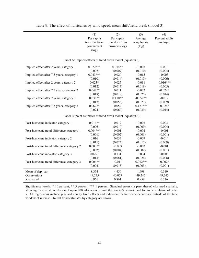
Table 9: The effect of hurricanes by wind speed, mean shift/trend break (model 3)

(1) (2) (3) (4)Per capita

transfers fromgovernment

(log)

Per capitatransfers frombusiness (log)

Averagewage/salary

(log)

Percent adultsemployed

Panel A: implied effects of trend break model (equation 3)

Implied effect after 2 years, category 1 0.022*** 0.014** -0.005 0.001(0.007) (0.007) (0.010) (0.004)

Implied effect after 7.5 years, category 1 0.043*** 0.020 -0.015 -0.003(0.010) (0.014) (0.015) (0.006)

Implied effect after 2 years, category 2 0.023* 0.027 -0.011 -0.016***(0.012) (0.017) (0.018) (0.005)

Implied effect after 7.5 years, category 2 0.042** 0.011 -0.022 -0.024*(0.018) (0.018) (0.025) (0.014)

Implied effect after 2 years, category 3 0.038** 0.110** -0.059** -0.012(0.017) (0.056) (0.027) (0.009)

Implied effect after 7.5 years, category 3 0.062** 0.052 -0.127*** -0.024*(0.024) (0.060) (0.039) (0.014)

Panel B: point estimates of trend break model (equation 3)

Post-hurricane indicator, category 1 0.014** 0.012 -0.002 0.003(0.006) (0.010) (0.009) (0.004)

Post-hurricane trend difference, category 1 0.004*** 0.001 -0.002 -0.001(0.001) (0.002) (0.001) (0.001)

Post-hurricane indicator, category 2 0.016 0.033 -0.007 -0.014(0.011) (0.024) (0.017) (0.009)

Post-hurricane trend difference, category 2 0.003** -0.003 -0.002 -0.001(0.002) (0.004) (0.002) (0.001)

Post-hurricane indicator, category 3 0.029* 0.131 -0.034 -0.008(0.015) (0.081) (0.024) (0.008)

Post-hurricane trend difference, category 3 0.004** -0.011 -0.012*** -0.002*(0.002) (0.015) (0.003) (0.001)

Mean of dep. var. 8.354 4.450 1.698 0.319Observations 49,245 40,027 49,245 49,245R-squared 0.961 0.861 0.958 0.216

Significance levels: * 10 percent, ** 5 percent, *** 1 percent. Standard errors (in parentheses) clustered spatially,allowing for spatial correlation of up to 200 kilometers around the county’s centroid and for autocorrelation of order5. All regressions include year and county fixed effects and indicators for hurricane occurrence outside of the timewindow of interest. Overall trend estimates by category not shown.

42

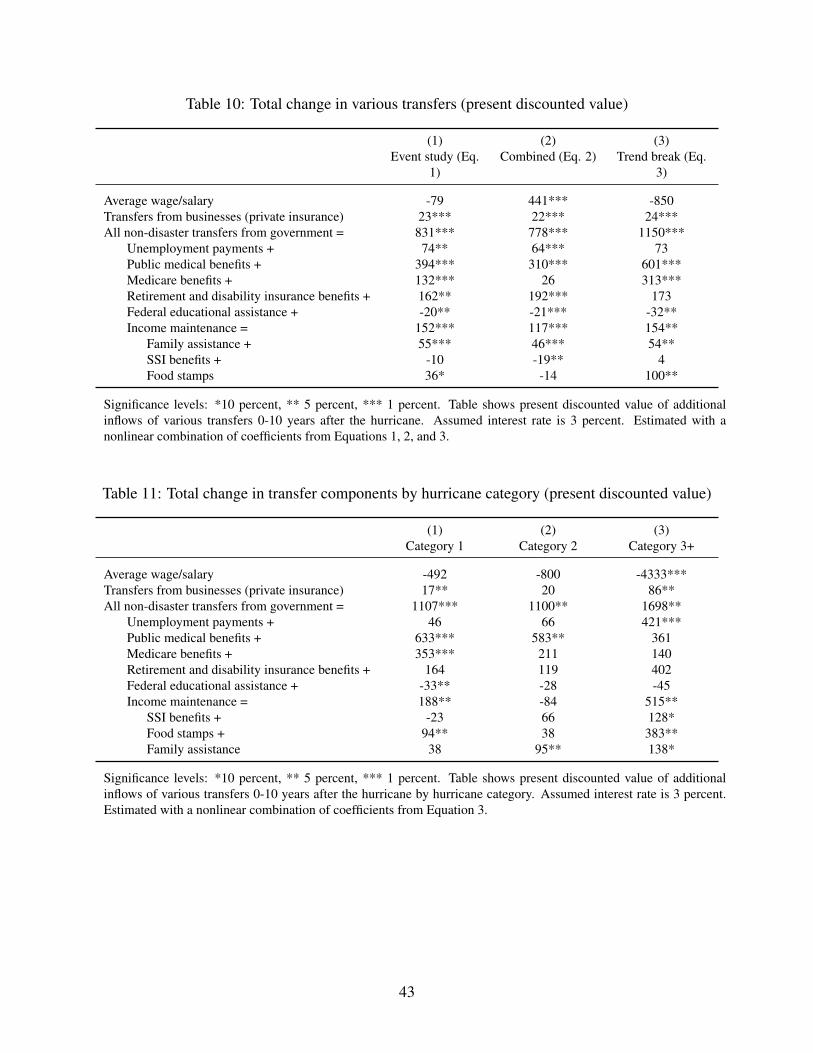
Table 10: Total change in various transfers (present discounted value)

(1) (2) (3)Event study (Eq.

1)Combined (Eq. 2) Trend break (Eq.

3)

Average wage/salary -79 441*** -850Transfers from businesses (private insurance) 23*** 22*** 24***All non-disaster transfers from government = 831*** 778*** 1150***

Unemployment payments + 74** 64*** 73Public medical benefits + 394*** 310*** 601***Medicare benefits + 132*** 26 313***Retirement and disability insurance benefits + 162** 192*** 173Federal educational assistance + -20** -21*** -32**Income maintenance = 152*** 117*** 154**

Family assistance + 55*** 46*** 54**SSI benefits + -10 -19** 4Food stamps 36* -14 100**

Significance levels: *10 percent, ** 5 percent, *** 1 percent. Table shows present discounted value of additionalinflows of various transfers 0-10 years after the hurricane. Assumed interest rate is 3 percent. Estimated with anonlinear combination of coefficients from Equations 1, 2, and 3.

Table 11: Total change in transfer components by hurricane category (present discounted value)

(1) (2) (3)Category 1 Category 2 Category 3+

Average wage/salary -492 -800 -4333***Transfers from businesses (private insurance) 17** 20 86**All non-disaster transfers from government = 1107*** 1100** 1698**

Unemployment payments + 46 66 421***Public medical benefits + 633*** 583** 361Medicare benefits + 353*** 211 140Retirement and disability insurance benefits + 164 119 402Federal educational assistance + -33** -28 -45Income maintenance = 188** -84 515**

SSI benefits + -23 66 128*Food stamps + 94** 38 383**Family assistance 38 95** 138*

Significance levels: *10 percent, ** 5 percent, *** 1 percent. Table shows present discounted value of additionalinflows of various transfers 0-10 years after the hurricane by hurricane category. Assumed interest rate is 3 percent.Estimated with a nonlinear combination of coefficients from Equation 3.

43