53

The Filtering of 3d textures

John Buchanan* Imager,

Department of Computer Science, University of British Columbia,

Vancouver, British Columbia Canada V6T 1W5

(604) 228-2218 e-mail buchanan@cs.ubc.ca

Abstract

Solid textures or textures defined over 3d have provided computer graphics with a new set of tools. Using these tools we can obtain effects which were difficult, if not impossible, to obtain with 2d texture mapping meth­ods. These textures are simple to implement using ei­ther scan line renderers or ray-tracers. Research in this area has focused on the generation and rendering of these textures with little consideration of the sampling and filtering problems which arise when these textures are used. The de-facto answer to the filtering prob­lem has been to clamp the signal so that no aliasing frequencies appear in the texture . Clamping a signal can cause variety of problems including energy loss and cross-spectrum energy leaks, we show how these arti­facts can arise in fairly simple examples. We propose a filtering method for filtering 3d textures which uses a box shaped kernel. A variety of filters can then be ap­plied over this box. This method is illustrated by using two kernels: the first aligned with the tangent plane of the surface; the second aligned along the ray from the intersection point to the eye.

Keywords: Solid texture, Aliasing, Clamping, Fil­tering, Quadrature rules.

Resume

Les textures definies en 3d procurent de nouveaux out­ils en infographie. En utilisant ces outils, il est possible de creer des effets difficiles, sinon impossibles a obtenir avec les techniques conventionnelles de mapping de tex­ture 2d . Ces textures 3d sont faciles a implanter dans des algorithmes de rendu a balagage et lancer de rayons. Jusqu'a present la recherche dans ce domaine etait con­centree sur la creation et le rendu de ces textures sans trop de consideration pour les problemes d'echantillon­nage et de filtrage qui surviennent lors de l'utilisation de ces textures. La solution au probleme de filtrage trop souvent adoptee etait de tronquer le signal, eliminant

• This research was partially supported by grants from the Natural Sciences and Engineering Research Counci l and from the Unive rsity of British Columbia and equipment donations from IBM

ainsi l'aliasing des hautes frequences. Tronquer un sig­nal peut causer plusieurs problemes allant d'une pede globale d 'energie a des pedes d'energies a travers le spectre. Nous montrons comment ces problemes peu­vent apparaltre dans de simples exemples. Nous pro­posons une technique de filtrage pour les textures 3d utilisant un noyau en forme de bolte. Plusieurs types de filtres peuvent alors etre employes sur cette boite. Cette technique est illustree avec deux noyaux: le pre­mier aligne au plan tangent ala surface; le second aligne le long du rayon defini par les positions de l'oeil et du point d 'intersection.

Mots cles: Texture en 3d, Aliasing, Tronquage, Filtrage, Regles de quadratures.

1 Introduction

In 1984 Fournier and Amanatides [grin84] and Perlin [perl84] talked about solid-textures. They defined a solid texture as a map which mapped !R3

-+

T{Pl , P2 , ... pp}, where Pi is some shading parameter . This definition is the one which we are going to use in this paper and it can equally include textures which are defined procedurally or textures which are digitized and the values interpolated from the nearest sample point . Gardner[gard84, gard85] presented a system for generat­ing transparency maps over ellipsoidal and quadric sur­faces. Some of these textures were defined as functions of !R3 and so they could be called 3d textures. Using these maps he modelled clouds and terrain for use in flight simulators.

In 1985 Perlin [perl85] and Peachey [peac85] inde­pendently introduced the term solid texture. Peachey used a variety of solid textures which show how solid textures could be generated and applied. In this paper he recognized that aliasing artifacts could arise but did not address the issue of anti-aliasing his textures. Per­lin proposed a system which used various transforma­tions of a solid noise function to model several textures. Recognizing the aliasing problems which could be intro­duced, he suggested clamping the texture based on the size of pixels.

In 1989 Lewis Qewi89] introduced more noise defor­mation algorithms, his main contribution was the in­troduction of Wiener interpolation for the use of noise

Graphics Interface '91

generation and manipulation. He did not address filter.­ing or sampling issues.

Perlin [perl89] extended the ideas presented in [perl85] . He used the noise function and its transforma­tions to deform object surfaces. These were rendered using a ray marching algorithm. Some of the objects he generates have a very high frequency surface. He uses these high frequency deformations to model fur-like tex­tures over object's surfaces. Again Perlin suggests the use of clamping to filter his images.

Kajiya and Kay [kaji89] presented a system for mod­eling and rendering fur like textures. Their texture parameters included colour, opacity, local coordinate frames, and shading parameters. In a typical applica.­tion a small texel of this texture would be generated. This generic texel would then be replicated over the surface of the object and rendered . Their texels are rendered by ray tracing through the texture. There is no discussion of potential aliasing problems or filtering solutions.

These two papers are interesting since they both pro­duce a similar set of 3d textures, but the process by which they arrive there is quite different. Kajiya and Kay set out to produce a model of fur which could be applied to objects, their approach was very focused on generating a texture which would have the visual char­acteristics of fur . Perlin on the other had uses the sur­face deformation algorithms to generate objects with increasingly higher frequency surfaces until he arrives at a model for a surface which resembles fur .

Volume rendering systems attempt to display tex­tures without using any geometric objects. There are two approaches to the problem: pixel based and voxel based. Pixel based volume rendering systems calculate the pixel value for a particular view. Most pixel based volume renderers use a ray tracing method with a line integral being performed along the ray. Voxel based volume rendering renderers calculate the influence that each voxel will have on the screen and update the pixels affected.

Upson and Keeler [ups088] present two methods for volume rendering, ray casting and voxel by voxel pro­cessing. Their ray casting technique steps through the data starting near the eye and traveling into the data. The evaluation of the colour coefficients in the voxel method is performed by clipping the voxel by a projec­tion of the pixel l into the data. Once the volume of the voxel which projects onto the pixel is computed a 3d integral is performed over this volume to evaluate the texture components and opacity. the pixel. The result­ing colour and opacity values are composited onto the pixel.

Westover [west90] presents a method for calculating the convolution of a reconstruction filter with a set of samples using a precomputed footprint . He first com­putes a generic footprint for a generic kernel, a sphere of radius 1. The footprint is generated by projecting the sphere onto the screen. For a discreet grid in the resulting circle the integral along z through2 the ker-

I Pixels are square in this context 2This calculation is done relative to the traditional eye coor­

dinate system

54

nel is computed. The resulting values represent the in­fluence that a particular data point will have over its footprint. When a view is selected the kernel surround­ing each sample Si is projected to its footprint :Ft and the generic footprint :Fg is transformed onto :Fi. This 'view-transformed' footprint can then be used to cal­culate which pixels are affected and in what manner. When this has been done for all the samples and the information appropriately accumulated the process is done.

Even though these methods perform filtered voxel rendering they are not appropriate for the display of textured objects in traditional computer graphics ap­plications. When we are displaying textured objects we are not interested in displaying all the texture data, but rather we are interested in calculating the texture coor­dinates of a point on the object.

1.1 Clamping

In 1982 Norton et al. [nort82] introduced a clamping method for the purpose of anti-aliasing, in this method the signal is clamped so that the aliasing frequencies are damped. In their paper the clamping method is devel­oped for signals whose frequency spectrum is known so that when the signal is clamped it can be replaced with its average. Towards the end of the paper they recognize that many textures must be dealt with for which there is no spectral information . In this case they suggest clamping the signal since in their experience this has lead to acceptable results. Even though clamping the signal in such a fashion will remove the aliasing frequen­cies it is easy to show that the energy of the resulting signal has been diminished .

Parseval's theorem [rose76] can be considered as a stating the conservation of energy between a signal s(t) and its Fourier transform F(s).

Thus replacing the function s(t) with a clamped func­

tion s' (t) which contains no frequencies greater than some frequency f o will remove energy from the right hand of the above equation since

J~oo IF(s)12dt = J~~o IF(sWds + f;o IF(sW ds

+ Jf~ IF(sW ds

> J~;o IF(sW ds

= J~oo IF(s')12

ds

and the energy we have removed from the signal is

The following example clearly illustrates the prob­lem. In this example we will use the function f(t) = )'~~I sin(nt). This function and a plot of If(tW are ;n'own in figure 1 for different values of N. The first plot illustrates the function f( t) on the left and on the

Graphics Interface '91

right a plot of If(t)1 2 for t E [-10,10] and N=20. In t he subsequent plots we show the result of clamping the signal for N = 15, and 10 respectively. The integral I = J~~o If(tWdt in these plots decreases significantly from plot to plot as the signal is progressively clamped.

Our criticism of clamping would not be complete without a set of images which show the effects of clamp­ing. In the image presented in figure 4 we show a plane which has been textured with the turbulence function presented by Perlin [perJ85].

pi:rel<.,j,.

f(u ,v, w)= L: 2Inlnoise(X2n,Y2n,Z2n)1 N=l

Near the horizon we have significant aliasing artifacts which we would like to get rid of. In the next image (figure 5) we see the result of clamping the texture . The texture on the plane near the horizon has been clamped to O.

A simple solution to this energy loss problem would be to compensate the rest of the texture components so that the energy is conserved. This can lead to chroma aliasing as the following example shows. Consider a two colour texture in which each colour signal is narrow band . If one of these signals has much higher spectral frequencies than the other, then the clamping of this signal will occur sooner on a perspective plane. If we try to compensate for the energy loss by transferring the energy from the clamped signal to the remaining signal we will have introduced an incorrect colour.

2 3D Box filter

The task of selecting a filter is a complex one. This se­lection process must select a filter whose cost and qual­ity matches t he requirements of the application . The computer graphics literature is full of good filters which can be used in a variety of 2d-texture filtering applica­tions . These filters provide users with a wide variety of features, strengths, and weaknesses. However when one considers the task of filtering a 3d-texture there is lit­tle to choose from even though in some applications the careful application of clamping may provide an adequate anti-aliasing technique. We wish to extend this choice of filters as part of an ongoing project to develop filtering techniques for 3d-textures. A first step approximation can be generated by performing a weighted integral

Y (Ph) = 1 F(x - Xo, Y - Yo, z - zo)t(x, Y, z)dv

over the rectangular volume IC. In this section we show t.he construction of two integral volumes IC, ur f and ICray •

The first integral volume IC.ur f is intended to be used for objects made of materials with a low trans­parency coefficient such as wood or stone. This volume is aligned with the tangent plane of the surface and typ­ically has a small dimension perpendicular to this plane. T he second volume ICray is intended to be used for ob­jects which exhibit some degree of translucency. This kernel is aligned with the ray from the object to the eye and can penetrate the object to arbitrary depths.

55

10

, r... .,. '.0' ~J~ 'J~ '.0' '0 .,

·10

1(1) l OO

J ' 0

.10 0.0, ..... , >.S, ¥S7 ' 0

.. 0

·100

1(11

N= 20 1 =124211

10

l ,

l ·1. ' "~r"'''JY' 'i"·' '0 .,

.10

sr,) lOO

1 '0 1 '·10 -6.'" ..... , >.S, .... '0

. '0

·100

1(11

N= 15 1= 93.4084

10

, ~ 11. "rO' ~J7" '''''V·,·, ,0

.,

.10

sr,) lOO

'0

.M .lA. ~/. ...,."' .... , >.S, ... , '0

· '0

·100

1(11

N= 10 1= 0.568259

Figure 1: Function s(t) and S(t)2 for N = {20, 15, I D}

where I is the integral f~o s(t?

Gra phics Inter face ' 91

2.1 A surface box filter

A simple yet effective approach to filtering 3d textures is to construct a box kernel which is aligned with the tan­gent plane of an object. We wish this box to be a good representation of the projection of the pixel onto the tangent plane. One such box is defined by calculating the box which is the projection of a circular pixel onto the tangent plane of the object. Note that when per­spective projection is being used most of the cones gen­erated by the projection of circular pixels on the screen will not be circular cones but elliptical cones. Since we are interested in a quick approximation we will approxi­mate these elliptical cones by the smallest circular cones which will enclose the elliptical cone. This approxima­tion will cause us to over filter some pixels. This overfil­tering may become apparent in the edge pixels of images with strong perspective.

Let Ph be the projection of the centre of the pixel onto the object. It is easy to show that Ph does not correspond to the centre of the projected ellipse, rather it lies on the major axis somewhere between the two foci. To calculate the box we need to calculate the vectors U and V which will lie parallel to the minor and major axis respectively. The centre of the box Pc is then calculated by computing the two quantities lLA and lLB which are the distances from the intersection point Ph to either end of the major axis respectively, as illustrated in figure 3. The centre of the box is the point Pc = UA ;UB U + Ph

Let R be a ray which is shot from the eye through the centre of the pixel. This ray and the circumference of the pixel define an elliptical cone. When we examine the angle between the line R and the edges of the cone we find that for every pixel there is a maximum angle 8 which can be calculated by

t:.z = viewz/resz , t:.y = viewz/resy

and d is the distance from the eye to the projection plane.

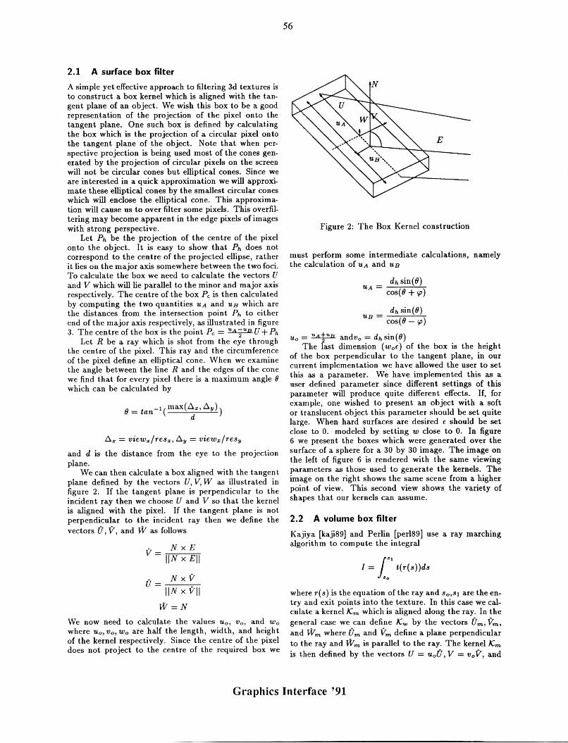
We can then calculate a box aligned with the tangent plane defined by the vectors U, V, W as illustrated in figure 2. If the tangent plane is perpendicular to the incident ray then we choose U and V so that the kernel is aligned with the pixel. If the tangent plane is not perpendicular to the incident ray then we define the vectors 0, V, and W as follows

V= N xE IIN x Ell

• NxV U = --=---

IIN x VII W=N

We now need to calculate the values lLo , V o , and W o

where lLo, V o , Wo are half the length, width, and height of the kernel respectively. Since the centre of the pixel does not project to the centre of the required box we

56

Figure 2: The Box Kernel construction

must perform some intermediate calculations, namely the calculation of lLA and lLB

dh sin(8) lLA =

cos(8 + tp)

dh sin(8) lLB =

cos(8-tp)

lL o = uA1uB andvo = dh sin(8) The last dimension (woe) of the box is the height

of the box perpendicular to the tangent plane, in our current implementation we have allowed the user to set this as a parameter. We have implemented this as a user defined parameter since different settings of this parameter will produce quite differen t effects. If, for example, one wished to present an object with a soft or translucent object this parameter should be set quite large. When hard surfaces are desired e should be set close to o. modeled by setting w close to o. In figure 6 we present the boxes which were generated over the surface of a sphere for a 30 by 30 image. The image on the left of figure 6 is rendered with the same viewing parameters as those used to generate the kernels. The image on the right shows the same scene from a higher point of view. This second view shows the variety of shapes that our kernels can assume.

2.2 A volume box filter

Kajiya [kaji89] and Perlin [perl89] use a ray marching algorithm to compute the integral

J" 1= t(r(s))ds

'0

where r(s) is the equation of the ray and So,SI are the en­try and exit points into the texture. In this case we cal­culate a kernel /Cm which is aligned along the ray. In the general case we can define /C W by the vectors Om, Vm, and Wm where Om and Vm define a plane perpendicular to the ray and W m is parallel to the ray. The kernel /Cm is then defined by the vectors U = lLoO, V = VO V, and

Graphics Interface '91

Figure 3: Calculation of UA and UB

w = IIr(s,);r(so)lIW. For most applications we would set uo/vo equal to the aspect ration of the display de­vice. In our current application the aspect ratio is 1 so we have set U o = Vo = dh sin(lI). Once we have defined the kernel we can simply use the quadrature methods described later to evaluate the integral.

In our current implementation the user can include in the parameters a spread factor which is applied to the U o and Vo parameters. By increasing/decreasing this spread factor we can produce over/under filtered images . The use of this parameter is illustrated in fig­ure 8

3 Evaluating the integral over the kernel

Given a function f : R3 -+ RI defined for all u, v, w in [-1,1] x [-1,1] x [-1 ,1] we wish to calculate a nu.merical approximation to the integral , we must also satIsfy the

constraint that fl fl fl dudvdw = 1. -I -I -I

I = ~ 11 11 11 f(u, v, w)du dvdw 8 -I -I -I

with a maximum error f. We can extend the com­mon adaptive quadrature method based on Simpson's method [burd81] to deal with this case as follows. From calculus we can rewrite the integral

8I=Iu=1

1

fu(u)du -I

where

Iv = fu(u) = fl fl f(u,v,w)dvdw

-I -I

= fl j(v) lu=uo dv

57

similarly

and

u = U o

v = Vo

u = U o

v = Vo

dw

= 11 f(u o, vo, w) - I

We now have three integrals in one variable. Each of these can be approximated using appropriate quad ra­ture rules. We have chosen to use adaptive Simpson's rule for the approximation of Iu and Iv. When the mag­nitude of ( is small compared to U o and Vo we use a order 3 gaussian approximation for the evaluation of I w. If ( is large then we use an adaptive Simpson's rule. For a more detailed discussion of quadrature rules please see [burd81].

4 Timing: or we knew you would ask this ques­tion

In those cases where a closed form solution for the con­volution integral can be calculated apriori timing should not be a problem, unless the evaluation of the resulting function proves to be to costly. In the general case the increased cost is dependent on the quadrature method(s) used in the convolution eval uation, on the function, and on the size of the kernel K. . In the situation where we have chosen to use Simpson's quadrature rule for the first two levels of the integral and a degree 3 Gaus­si an approximation for the last integral. The mini­mum number of texture evaluations required would be 5 x 5 x 3 = 75. When adaptive quadrature methods are being used the texture evaluations could become much greater . In general function s with high frequency com­ponents will cause these adaptive quadrature methods to work harder. For many applications it may prove sufficient to use a fixed quadrature method for all our integrals. .

Using a network of 4 IBM RS/6000 workstatlOns and 13 SGI iris workstations the images in figures 7 and 8 were rendered at a resolution of 320 by 240. The point sampled version of the marble block in figure 8 required 45 seconds for display. Using a degree 3 Gaussian ap­proximation for the integrals the display time was ~ min­utes. When we used adaptive quadrature for the dIsplay of this image the display time was 6 minutes.

5 Examples

Figure 7 shows a progression of a sphere textured with the texture function

{

(1,1,1) T(p) = (0,1,0)

(t(IOx, IOy, 10z), 0, 0)

if IIplI > 0.9 if 0.9 ~ IIplI > 0.7 otherwise

Graphics Interface '91

( = .1 (= .4 ( = .7 (= .2 (= .5 ( = .8 ( = .3 (= .6 ( - .9

Table 1: Parameters for figure 7

Box filter Bartlett filter Volume filter

(= 0.01 ( - 0.01 (- 0.025 spread = 1.0 spread = 1.0 spread = 1.0 (= 0.01 ( = 0.01 ( = 0.100 spread = 2.0 spread = 2.0 spread = 1.0 (= 0.01 ( - 0.01 ( - 0.200 spread = 4.0 spread = 4.0 spread = 1.0

Table 2: Parameters for figure 8

where t(x , y, z) = turbulence(x, y, z) is the turbulence function proposed by perlin [perl85] . Nine versions of the sphere are presented with various penetration depths for the integral volume Kray . The ( values for this figure are presented in table 1 In figure 8 we illustrate a marble block whose size is 2 x 2 x 2 x rendered with various filter parameters. In the first column we have a surface box filter, in the second column we have an application of a bartlett filter to the same box, and in the third column we apply a volume filter to the texture . In table 2 table we outline the parameters of the filters in this image.

6 Conclusion

In this paper we have shown that there is a need for 3d texture filtering. We illustrated some of the shortcom­ings of clamping as a filtering or anti-aliasing technique. We proposed the use of filters evaluated over rectangu­lar boxes. These boxes allow the application of arbitrary filters over rectangular volumes of the texture. We il­lustrated the use of these boxes with two filter kernels: the first, a kernel aligned with the tangent plane of the object; the second, a kernel oriented with the ray. We presented a set of images which illustrate the applica­tions of these techniques.

7 Future work

This work is a first step in a project whose goal is to develop adequate filters for 3d textures. The author is very much challenged by the idea of extending the con­stant cost 2d filtering algorithm presented by Fournier and Fiume [four88].

Acknowledgements

Alain Fournier was an excellent challenger and gener­ator of ideas. Pierre Poulin did not believe anything I said. Peter Cahoon again became the lab photog­rapher. The members of the Imager and GraFiC lab did not complain (to much) when I was using all the

58

machines. Ruhamah provided a constant reminder of reality. Mary Jane constantly encouraged me. To all of you THANKS!!!!!!!

References

[burd81] R . Burden, J. Faires, and A . Reynolds. Nu­merical Analysis, Second edition. PWS Pub­lishers, Boston, Massachusetts, 1981.

[iour88] Alain Fournier and Eugene Fiume. "Constant­Time Filtering with Space-Variant Kernels". Computer Graphics (SIGGRAPH '88 Proceed­ings) , Vo!. 22, No. 4, pp. 229-238, August 1988.

[gard84] Geoffrey Y. Gardner. "Simulation of Natu­ral Scenes Using Textured Quadric Surfaces". Computer Graphics (SIGGRAPH '84 Proceed­ings), Vo!. 18, No. 3, pp. 11-20, July 1984.

[gard85] G.Y. Gardner. "Visual Simulation of Clouds". Computer Graphics (SIGGRAPH '85 Proceed­ings), Vo!. 19, No. 3, pp. 297-303, J uly 1985.

[grin84] D. Grindal. "The Stochastic Creation of Tree Images" . Master's thesis, University of Toronto, Toronto, Canada, 1984.

[kaji89] James T. Kajiya and Timothy L. Kay. "Ren­dering Fur with Three Dimensional Textures". Computer Graphics (SIGGRAPH '89 Proceed­ings) , Vo!. 23, No. 3, pp. 271-280, July 1989.

~ewi89] J . P . Lewis. "Algorithms for Solid Noise Syn­thesis" . Computer Graphics (SIGGRAPH '89 Proceedings), Vo!. 23, No. 3, pp. 263-270, July 1989.

[nort82] A. Norton, A.P. Rockwood, and P.T. Skol­moski. "Clamping: A Method of Antialias­ing Textured Surfaces by Bandwidth Limit­ing in Object Space". Computer Graphics (SIGGRAPH '82 Proceedings), Vo!. 16, No. 3, pp. 1-8, July 1982.

[peac85] D .R. Peachey. "Solid Texturing of Complex Surfaces". Computer Graphics (SIGGRAPH '85 Proceedings), Vo!. 19, No. 3, pp. 279-286 , July 1985.

[pe rl84] K . Perlin. "A tutorial on texture mapping". Siggraph course., July 1984.

[perl85] K . Perlin. "An Image Synthesizer" . Com­puter Graphics (SIGGRAPH '85 Proceedings), Vo!. 19, No. 3, pp. 287-296, July 1985.

[perl89] Ken Perlin and Eric M. Hoffert. "Hypertex­ture" . Computer Graphics (SIGGRAPH '89 Proceedings), Vo!. 23, No. 3, pp. 253-262, July 1989.

[rose76] A . Rosenfeld and A. Kak . Digital Picture Pro­cessing. Academic publishers, New York, New York, 1976.

Graphics Interface '91

59

[upso88] Craig Upson and Michael Keeler. "V- * BUFFER: Visible Volume Rendering". Com-puter Graphics (SIGGRAPH '88 Proceedings), Vo!. 22, No. 4, pp. 59- 64, August 1988.

[west90] Lee Westover. "Footprint Evaluation for Vol­ume Rendering". Computer Graphics (SJG­GRAPH '90 Proceedings), Vo!. 24, No. 4 , pp. 367-376, August 1990.

Figure 4: Point sampled turbulence function Figure 5: Clamped turbulence function

Figure 6: Kernels generated by the system

Graphics Interface '91

60

Figure 7: Filter aligned with the ray

Figure 8: Different filter results

Graphics Interface '91