the expression of uncertainty and confidence in measurement · 2.6 in order to quantify the...
TRANSCRIPT
United Kingdom Accreditation Service, 21-47 High Street, Feltham, Middlesex, TW13 4UNWebsite: www.ukas.com Publication requests Tel: +44 (0) 20 8917 8421 Fax: +44 (0) 20 8917 8500
© United Kingdom Accreditation Service. UKAS Copyright exists in all UKAS publications
PAGE 1 OF 82 EDITION 2 | JANUARY 2007
M3003 EDITION 2 | JANUARY 2007
The Expression of Uncertainty and Confidence inMeasurement JH 2007
CONTENTS
SECTION PAGE
1 Introduction 22 Overview 43 More detail 104 Type A evaluation of standard uncertainty 185 Type B evaluation of standard uncertainty 206 Reporting of results 217 Step by step procedure for evaluation of measurement uncertainty 22
Appendix A Best measurement capability 26Appendix B Deriving a coverage factor for unreliable input quantities 28Appendix C Dominant non-Gaussian Type B uncertainty 31Appendix D Derivation of the mathematical model 34Appendix E Some sources of error and uncertainty in electrical calibrations 37Appendix F Some sources of error and uncertainty in mass calibrations 42Appendix G Some sources of error and uncertainty in temperature calibrations 44Appendix H Some sources of error and uncertainty in dimensional calibrations 45Appendix J Some sources of error and uncertainty in pressure calibration using DWTs 46Appendix K Examples of application for calibration 48Appendix L Expression of uncertainty for a range of values 66Appendix M Assessment of compliance with specification 69Appendix N Uncertainties for test results 74Appendix P Electronic data processing 78Appendix Q Symbols 80Appendix R References 82

THE EXPRESSION OF UNCERTAINTY AND CONFIDENCE IN MEASUREMENT M3003 | EDITION 2 | JANUARY 2007
United Kingdom Accreditation Service, 21-47 High Street, Feltham, Middlesex, TW13 4UNWebsite: www.ukas.com Publication requests Tel: +44 (0) 20 8917 8421 Fax: +44 (0) 20 8917 8500
© United Kingdom Accreditation Service. UKAS Copyright exists in all UKAS publications
PAGE 2 OF 82
1 INTRODUCTION
1.1 The general requirements that testing and calibration laboratories have to meet if they wish todemonstrate that they operate to a quality system, are technically competent and are able togenerate technically valid results are contained within ISO/IEC 17025:2005. This internationalstandard forms the basis for international laboratory accreditation and in cases of differences ininterpretation remains the authoritative document at all times. M3003 is not intended as aprescriptive document, and does not set out to introduce additional requirements to those inISO/IEC 17025:2005 but to provide amplification and guidance on the current requirements withinthe international standard.
1.2 The purpose of these guidelines is to provide policy on the evaluation and reporting ofmeasurement uncertainty for testing and calibration laboratories. Related topics, such asevaluation of compliance with specifications, are also included. A number of worked examples areincluded in order to illustrate how practical implementation of the principles involved can beachieved.
1.3 The guidance in this document is based on information in the Guide to the Expression ofUncertainty in Measurement [1], hereinafter referred to as the GUM. M3003 is consistent with theGUM both in methodology and terminology. It does not, however, preclude the use of othermethods of uncertainty evaluation that may be more appropriate to a specific discipline. Forexample, the use of Bayesian statistics is becoming recognised as being particularly useful incertain areas of testing.
1.4 M3003 is aimed both at the beginner and at those more experienced in the subject ofmeasurement uncertainty. In order to address the needs of an audience with a wide spectrum ofexperience, the subject is introduced in relatively straightforward terms and gives details of thebasic concepts involved. Cross-references are made to a number of Appendices, where moredetailed information is presented for those who wish to obtain a deeper understanding of thesubject.
1.5 Edition 2 of M3003 is a complete revision of the previous issue and it is impractical to list all thechanges in detail. Some of the more notable changes or additions are as follows:
1.5.1 An overview of the basic concepts relating to uncertainty evaluation is given in Section 2 tointroduce these ideas to those new to the subject. This is then expanded upon in Section 3, whichgives more formal detail.
1.5.2 ISO/IEC 17025:2005 criteria, which were not in place when Edition 1 was published, have beenconsidered.
1.5.3 A section on derivation of the measurement model has been included.
1.5.4 Concepts are accompanied by simple worked examples as they are introduced.
1.5.5 A number of diagrams illustrating the concepts have been included.
1.5.6 Further detail has been included regarding dominant contributions.
1.5.7 The subject of compliance with specification has been explored in more detail.

THE EXPRESSION OF UNCERTAINTY AND CONFIDENCE IN MEASUREMENT M3003 | EDITION 2 | JANUARY 2007
United Kingdom Accreditation Service, 21-47 High Street, Feltham, Middlesex, TW13 4UNWebsite: www.ukas.com Publication requests Tel: +44 (0) 20 8917 8421 Fax: +44 (0) 20 8917 8500
© United Kingdom Accreditation Service. UKAS Copyright exists in all UKAS publications
PAGE 3 OF 82
1.5.8 The worked examples have been reviewed and minor amendments have been made asnecessary.
1.5.9 A new example, relating to pressure calibration using a deadweight tester, has been added,together with a section describing the sources of uncertainty for these measurements.
1.5.10 Hyperlinks have been included between various sections of the document.
1.5.11 Analytical concepts such as Monte Carlo simulation and Bayesian statistics have been introduced.
1.6 No further changes of any significance will be made to M3003 Edition 2 during its lifetime.However, minor text modifications of an editorial nature may be made if the need is identified. Anysuch changes will be listed below.
Date Details of amendment
2 January 2007 First issue of M3003 Edition 28 January 2007 Amendment A1: Minor text corrections made; paragraph numbers in
Appendix M corrected; cross-reference on Page 16 corrected.30 January 2007 Amendment A2: Probability distribution in second line of uncertainty budget
K8.15 corrected; reference to LAB14 on page 82 updated.22 February 2008 Amendment A3: Sensitivity coefficient CS in K7.6 corrected from 0.200 ºC/μV
to CS = 0.189 ºC/μV. Resolution in K8.14 corrected from 20 Pa to 200 Pa.Repeated line removed in K8.1.
THE EXPRESSION OF UNCERTAINTY AND CONFIDENCE IN MEASUREMENT M3003 | EDITION 2 | JANUARY 2007
United Kingdom Accreditation Service, 21-47 High Street, Feltham, Middlesex, TW13 4UNWebsite: www.ukas.com Publication requests Tel: +44 (0) 20 8917 8421 Fax: +44 (0) 20 8917 8500
© United Kingdom Accreditation Service. UKAS Copyright exists in all UKAS publications
PAGE 4 OF 82
2 OVERVIEW
2.1 In many aspects of everyday life, we are accustomed to the doubt that arises when estimating howlarge or small things are. For example, if somebody asks, “what do you think the temperature ofthis room is?” we might say, “it is about 23 degrees Celsius”. The use of the word “about” impliesthat we know the room is not exactly 23 degrees, but is somewhere near it. In other words, werecognise that there is some doubt about the value of the temperature that we have estimated.
2.2 We could, of course, be a bit more specific. We could say, “it is 23 degrees Celsius give or take acouple of degrees”. The term “give or take” implies that there is still doubt about the estimate, butnow we are assigning limits to the extent of the doubt. We have given some quantitativeinformation about the doubt, or uncertainty, of our estimate.
2.3 It is also quite reasonable to assume that we may be more sure that our estimate is within, say, 5degrees of the “true” room temperature than we are that it is within 2 degrees. The larger theuncertainty we assign, the more confident we are that it encompasses the “true” value. Hence, for agiven situation, the uncertainty is related to the level of confidence.
2.4 So far, our estimate of the room temperature has been based on a subjective evaluation. This isnot entirely a guess, as we may have experience of exposure to similar and known environments.However, in order to make a more objective measurement it is necessary to make use of ameasuring instrument of some kind; in this case we can use a thermometer.
2.5 Even if we use a measuring instrument, there will still be some doubt, or uncertainty, about theresult. For example we could ask:
“Is the thermometer accurate?”
“How well can I read it?”
“Is the reading changing?”
“I am holding the thermometer in my hand. Am I warming it up?”
“The relative humidity in the room can vary considerably. Will this affect my results?”
“Does it matter where in the room I take the measurement?”
All these factors, and possibly others, may contribute to the uncertainty of our measurement of theroom temperature.
2.6 In order to quantify the uncertainty of the room temperature measurement we will therefore have toconsider all the factors that could influence the result. We will have to make estimates of thepossible variations associated with these influences. Let us consider the questions posed above.
THE EXPRESSION OF UNCERTAINTY AND CONFIDENCE IN MEASUREMENT M3003 | EDITION 2 | JANUARY 2007
United Kingdom Accreditation Service, 21-47 High Street, Feltham, Middlesex, TW13 4UNWebsite: www.ukas.com Publication requests Tel: +44 (0) 20 8917 8421 Fax: +44 (0) 20 8917 8500
© United Kingdom Accreditation Service. UKAS Copyright exists in all UKAS publications
PAGE 5 OF 82
2.7 Is the thermometer accurate?
2.7.1 In order to find out, it will be necessary to compare it with a thermometer whose accuracy is betterknown. This thermometer, in turn, will have to be compared with an even better characterised one,and so on. This leads to the concept of traceability of measurements, whereby measurements at alllevels can be traced back to agreed references. In most cases, ISO/IEC17025:2005 requires thatmeasurements are traceable to SI units. This is usually achieved by an unbroken chain ofcomparisons to a national metrology institute, which maintains measurement standards that aredirectly related to SI units.
In other words, we need a traceable calibration. This calibration itself will provide a source ofuncertainty, as the calibrating laboratory will assign a calibration uncertainty to the reported values.When used in a subsequent evaluation of uncertainty, this is often referred to as the importeduncertainty.
2.7.2 In terms of the thermometer accuracy, however, a traceable calibration is not the end of the story.Measuring instruments change their characteristics as time goes by. They “drift”. This, of course, iswhy regular recalibration is necessary. It is therefore important to evaluate the likely change sincethe instrument was last calibrated.
If the instrument has a reliable history it may be possible to predict what the reading error will be ata given time in the future, based on past results, and apply a correction to the reading. Thisprediction will not be perfect and therefore an uncertainty on the corrected value will be present. Inother cases, the past data may not indicate a reliable trend, and a limit value may have to beassigned for the likely change since the last calibration. This can be estimated from examination ofchanges that occurred in the past. Evaluations made using these methods yield the uncertainty dueto secular stability, or changes with time, of the instrument. This is also known as “drift”.
2.7.3 There are other possible influences relating to the thermometer accuracy. For example, supposewe have a traceable calibration, but only at 15 °C, 20 °C and 25 °C. What does this tell us about itsindication error at 23 °C?
In such cases we will have to make an estimate of the error, perhaps using interpolation betweenpoints where calibration data is available. This is not always possible as it depends on themeasured data being such that accurate interpolation is practical. It may then be necessary to useother information, such as the manufacturer’s specification, to evaluate the additional uncertaintythat arises when the reading is not directly at a point that has been calibrated.
2.8 How well can I read it?
2.8.1 There will inevitably be a limit to which we can resolve the reading we observe on the thermometer.If it is a liquid-in-glass thermometer, this limit will often be imposed by our ability to interpolatebetween the scale graduations. If it is a thermometer with a digital readout, the finite number ofdigits in the display will define the limit.
2.8.2 For example, suppose the last digit of a digital thermometer can change in steps of 0.1 °C. Thereading happens to be 23.4 °C. What does this mean in terms of uncertainty?
The reading is a rounded representation of an infinite continuum of underlying values that thethermometer would indicate if it had more digits available. In the case of a reading of 23.4 °C, thismeans that the underlying value cannot be less than 23.35 °C, otherwise the rounded readingwould be 23.3 °C. Similarly, the underlying value cannot be more than 23.45 °C, otherwise therounded reading would be 23.5 °C.
A reading of 23.4 °C therefore means that the underlying value is somewhere between 23.35 °Cand 23.45 °C. In other words, the 0.1 °C resolution of the display has caused a rounding errorsomewhere between –0.05 °C and +0.05 °C. As we have no way of knowing where in this range

THE EXPRESSION OF UNCERTAINTY AND CONFIDENCE IN MEASUREMENT M3003 | EDITION 2 | JANUARY 2007
United Kingdom Accreditation Service, 21-47 High Street, Feltham, Middlesex, TW13 4UNWebsite: www.ukas.com Publication requests Tel: +44 (0) 20 8917 8421 Fax: +44 (0) 20 8917 8500
© United Kingdom Accreditation Service. UKAS Copyright exists in all UKAS publications
PAGE 6 OF 82
the underlying value is, we have to assume the rounding error is zero with limits of ± 0.05 °C.
2.8.3 It can therefore be seen that there will always be an uncertainty of ± half of the change representedby one increment of the last displayed digit. This does not only apply to digital displays; it appliesevery time a number is recorded. If we write down a rounded result of 123.456, we are imposing anidentical effect by the fact that we have recorded this result to three decimal places, and anuncertainty of ± 0.0005 will arise.
2.8.4 This source of uncertainty is frequently referred to as “resolution”, however it is more correctly thenumeric rounding caused by finite resolution.
2.9 Is the reading changing?
2.9.1 Yes, it probably is! Such changes may be due to variations in the room temperature itself,variations in the performance of the thermometer and variations in other influence quantities, suchas the way we are holding the thermometer.
So what can be done about this?
2.9.2 We could, of course, just record one reading and say that it is the measured temperature at a givenmoment and under particular conditions. This would have little meaning, as we know that the nextreading, a few seconds later, could well be different. So which is “correct”?
2.9.3 In practice, we will probably take an average of several measurements in order to obtain a morerealistic reading. In this way, we can “smooth out” the effect of short-term variations in thethermometer indication. The average, or arithmetic mean, of a number of readings can often becloser to the “true” value than any individual reading is.
2.9.4 However, we can only take a finite number of measurements. This means that we will never obtainthe “true” mean value that would be revealed if we could carry out an infinite (or very large) numberof measurements. There will be an unknown error – and therefore an uncertainty – represented bythe difference from our calculated mean value and the underlying “true” mean value.
2.9.5 This uncertainty cannot be evaluated using methods like those we have already considered. Upuntil now, we have looked for evidence, such as calibration uncertainty and secular stability. Wehave considered what happens with finite resolution by logical reasoning. The effects of variationbetween readings cannot be evaluated like this, because there is no background informationavailable upon which to base our evaluation.
2.9.5 The only information we have is a series of readings and a calculated average, or mean, value. Wetherefore have to use a statistical approach to determine how far our calculated mean could beaway from the “true” mean. These statistics are quite straightforward and give us the uncertaintyassociated with the repeatability (or, more correctly, non-repeatability) of our measurements. Thisuncertainty is referred to as the experimental standard deviation of the mean. For the sake ofbrevity, this is often referred to as simply the standard deviation of the mean.
NOTE
In earlier textbooks on the subjects of uncertainty or statistics, this may be referred to as the standard error of the mean.
2.9.6 It is often convenient to regard the calculation of the standard deviation of the mean as a two-stageprocess, and it can be performed easily on most scientific calculators.
2.9.7 First we calculate the estimated standard deviation using the values we have measured. Thisfacility is indicated on most calculators by the function key xσn-1. On some calculators it is identifiedas s(x) or simply s.
THE EXPRESSION OF UNCERTAINTY AND CONFIDENCE IN MEASUREMENT M3003 | EDITION 2 | JANUARY 2007
United Kingdom Accreditation Service, 21-47 High Street, Feltham, Middlesex, TW13 4UNWebsite: www.ukas.com Publication requests Tel: +44 (0) 20 8917 8421 Fax: +44 (0) 20 8917 8500
© United Kingdom Accreditation Service. UKAS Copyright exists in all UKAS publications
PAGE 7 OF 82
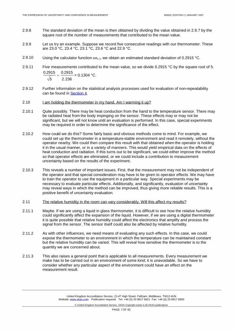
2.9.8 The standard deviation of the mean is then obtained by dividing the value obtained in 2.9.7 by thesquare root of the number of measurements that contributed to the mean value.
2.9.9 Let us try an example. Suppose we record five consecutive readings with our thermometer. Theseare 23.0 °C, 23.4 °C, 23.1 °C, 23.6 °C and 22.9 °C.
2.9.10 Using the calculator function xσn-1, we obtain an estimated standard deviation of 0.2915 °C.
2.9.11 Five measurements contributed to the mean value, so we divide 0.2915 °C by the square root of 5.
236.2
2915.0
5
2915.0 = 0.1304 °C.
2.9.12 Further information on the statistical analysis processes used for evaluation of non-repeatabilitycan be found in Section 4.
2.10 I am holding the thermometer in my hand. Am I warming it up?
2.10.1 Quite possibly. There may be heat conduction from the hand to the temperature sensor. There maybe radiated heat from the body impinging on the sensor. These effects may or may not besignificant, but we will not know until an evaluation is performed. In this case, special experimentsmay be required in order to determine the significance of the effect.
2.10.2 How could we do this? Some fairly basic and obvious methods come to mind. For example, wecould set up the thermometer in a temperature-stable environment and read it remotely, without theoperator nearby. We could then compare this result with that obtained when the operator is holdingit in the usual manner, or in a variety of manners. This would yield empirical data on the effects ofheat conduction and radiation. If this turns out to be significant, we could either improve the methodso that operator effects are eliminated, or we could include a contribution to measurementuncertainty based on the results of the experiment.
2.10.3 This reveals a number of important issues. First, that the measurement may not be independent ofthe operator and that special consideration may have to be given to operator effects. We may haveto train the operator to use the equipment in a particular way. Special experiments may benecessary to evaluate particular effects. Additionally, and significantly, evaluation of uncertaintymay reveal ways in which the method can be improved, thus giving more reliable results. This is apositive benefit of uncertainty evaluation.
2.11 The relative humidity in the room can vary considerably. Will this affect my results?
2.11.1 Maybe. If we are using a liquid in glass thermometer, it is difficult to see how the relative humiditycould significantly affect the expansion of the liquid. However, if we are using a digital thermometerit is quite possible that relative humidity could affect the electronics that amplify and process thesignal from the sensor. The sensor itself could also be affected by relative humidity.
2.11.2 As with other influences, we need means of evaluating any such effects. In this case, we couldexpose the thermometer to an environment in which the temperature can be maintained constantbut the relative humidity can be varied. This will reveal how sensitive the thermometer is to thequantity we are concerned about.
2.11.3 This also raises a general point that is applicable to all measurements. Every measurement wemake has to be carried out in an environment of some kind; it is unavoidable. So we have toconsider whether any particular aspect of the environment could have an effect on themeasurement result.

THE EXPRESSION OF UNCERTAINTY AND CONFIDENCE IN MEASUREMENT M3003 | EDITION 2 | JANUARY 2007
United Kingdom Accreditation Service, 21-47 High Street, Feltham, Middlesex, TW13 4UNWebsite: www.ukas.com Publication requests Tel: +44 (0) 20 8917 8421 Fax: +44 (0) 20 8917 8500
© United Kingdom Accreditation Service. UKAS Copyright exists in all UKAS publications
PAGE 8 OF 82
2.11.4 The significance of a particular aspect of the environment has to be considered in the light of thespecific measurement being made. It is difficult to see how, for example, gravity could significantlyinfluence the reading on a digital thermometer. However, it certainly will affect the results obtainedon a precision weighing machine that might be right next to the thermometer!
2.11.5 The following environmental effects are amongst the most commonly encountered whenconsidering measurement uncertainty:
TemperatureRelative humidityBarometric pressureElectric or magnetic fieldsGravityElectrical supplies to measuring equipmentAir movementVibrationLight and optical reflections
Furthermore, some of these influences may have little effect as long as they remain constant, butcould affect measurement results when they start changing. Rate of change of temperature can beparticularly important.
2.11.6 It can be seen by now that understanding of a measurement system is important in order to identifyand quantify the various uncertainties that can arise in a measurement situation. Conversely,analysis of uncertainty can often yield a deeper understanding of the system and reveal ways inwhich the measurement process can be improved. This leads on to the next question…
2.12 Does it matter where in the room I make the measurement?
2.12.1 It depends what we are trying to measure! Are we interested in the temperature at a specificlocation? Or the average of the temperatures encountered at any location within the room? Or theaverage temperature at bench height?
2.12.2 There may be further, related questions. For example, do we require the temperature at a particulartime of day, or the average over a specific period of time?
2.12.3 Such questions have to be asked, and answered, in order that we can devise an appropriatemeasurement method that gives us the information we require. Until we know the details of themethod, we are not in a position to evaluate the uncertainties that will arise from that method.
2.12.4 This leads to what is perhaps the most important question of all, one that should be asked beforewe even start with our evaluation of uncertainty:
2.13 “What exactly is it that I am trying to measure?”
2.13.1 Until this question is answered, we are not in a position to carry out a proper evaluation of theuncertainty. The particular quantity subject to measurement is known as the measurand. In order toevaluate the uncertainty in a measurement system, we must define the measurand otherwise weare not in a position to know how a particular influence quantity affects the value we obtain for it.
2.13.2 The implication of this is that there has to be a defined relationship between the influence quantitiesand the measurand. This relationship is known as the mathematical model. This is an equation thatdescribes how each influence quantity affects the value assigned to the measurand. In effect, it is adescription of the measurement process. Further details about the derivation of the mathematicalmodel can be found in Appendix D. A proper analysis of this process also gives the answer toanother important question:
THE EXPRESSION OF UNCERTAINTY AND CONFIDENCE IN MEASUREMENT M3003 | EDITION 2 | JANUARY 2007
United Kingdom Accreditation Service, 21-47 High Street, Feltham, Middlesex, TW13 4UNWebsite: www.ukas.com Publication requests Tel: +44 (0) 20 8917 8421 Fax: +44 (0) 20 8917 8500
© United Kingdom Accreditation Service. UKAS Copyright exists in all UKAS publications
PAGE 9 OF 82
2.14 “Am I actually measuring the quantity that I thought I was measuring?”
2.14.1 Some measurement systems are such that the result would be only an approximation to the “true”value, even if no other uncertainties were present, because of assumptions and approximationsinherent in the method. The model should include any such assumptions and thereforeuncertainties that arise from them will be accounted for in the analysis.
2.15 Summary
2.15.1 This section of M3003 has given an overview of uncertainty and some insights into howuncertainties might arise. It has shown that we have to know our measurement system and the wayin which the various influences can affect the result. It has also shown that analysis of uncertaintycan have positive benefits in that it can reveal where enhancements can be made to measurementmethods, hence improving the reliability of measurement results.
2.15.2 The following sections of M3003 explore the issues identified in this overview in more detail.
THE EXPRESSION OF UNCERTAINTY AND CONFIDENCE IN MEASUREMENT M3003 | EDITION 2 | JANUARY 2007
United Kingdom Accreditation Service, 21-47 High Street, Feltham, Middlesex, TW13 4UNWebsite: www.ukas.com Publication requests Tel: +44 (0) 20 8917 8421 Fax: +44 (0) 20 8917 8500
© United Kingdom Accreditation Service. UKAS Copyright exists in all UKAS publications
PAGE 10 OF 82
3 IN MORE DETAIL…
3.1 The Overview section of M3003 has provided an introduction to the subject of uncertainty evaluationand has explored a number of the issues involved. This section provides a more formal description ofthese processes, using terminology consistent with that in the GUM.
3.2 A quantity (Q) is a property of a phenomenon, body or substance to which a magnitude can beassigned. The purpose of a measurement is to assign a magnitude to the measurand; the quantityintended to be measured. The assigned magnitude is considered to be the best estimate of the valueof the measurand.
3.3 The uncertainty evaluation process will encompass a number of influence quantities that affect theresult obtained for the measurand. These influence, or input, quantities are referred to as X and theoutput quantity, i.e., the measurand, is referred to as Y.
3.4 As there will usually be several influence quantities, they are differentiated from each other by thesubscript i, So there will be several input quantities called Xi, where i represents integer values from 1to N, N being the number of such quantities. In other words, there will be input quantities of X1, X2, …XN.
3.5 Each of these input quantities will have a corresponding value. For example, one quantity might be thetemperature of the environment – this will have a value, say 23 °C. A lower-case “x” represents thevalues of the quantities. Hence the value of X1 will be x1, that of X2 will be x2, and so on.
3.6 The purpose of the measurement is to determine the value of the measurand, Y. As with the inputuncertainties, the value of the measurand is represented by the lower-case letter, i.e. y. Theuncertainty associated with y will comprise a combination of the input, or xi, uncertainties. One of thefirst steps is to establish the mathematical relationship between the values of the input quantities, xi,and that of the measurand, y. This process is examined in Appendix D.
3.7 The values xi of the input quantities Xi will all have an associated uncertainty. This is referred to asu(xi), i.e. “the uncertainty of xi”. These values of u(xi) are known as standard uncertainties – but moreon this shortly.
3.8 Some uncertainties, particularly those associated with the determination of repeatability, have to beevaluated by statistical methods. Others have been evaluated by examining other information, such asdata in calibration certificates, evaluation of long-term drift, consideration of the effects of environment,etc.
3.9 The GUM differentiates between statistical evaluations and those using other methods. It categorisesthem into two types – Type A and Type B.
3.10 A Type A evaluation of uncertainty is carried out using statistical analysis of a series of observations.Further details about Type A evaluations can be found in Section 4.
3.11 A Type B evaluation of uncertainty is carried out using methods other than statistical analysis of aseries of observations. Further details about Type B evaluations can be found in Section 5.
3.12 In paragraph 3.3.4 of the GUM it is stated that the purpose of the Type A and Type B classification is toindicate the two different ways of evaluating uncertainty components, and is for convenience indiscussion only. Whether components of uncertainty are classified as `random' or `systematic' in relationto a specific measurement process, or described as Type A or Type B depending on the method ofevaluation, all components regardless of classification are modelled by probability distributions quantifiedby variances or standard deviations.
THE EXPRESSION OF UNCERTAINTY AND CONFIDENCE IN MEASUREMENT M3003 | EDITION 2 | JANUARY 2007
United Kingdom Accreditation Service, 21-47 High Street, Feltham, Middlesex, TW13 4UNWebsite: www.ukas.com Publication requests Tel: +44 (0) 20 8917 8421 Fax: +44 (0) 20 8917 8500
© United Kingdom Accreditation Service. UKAS Copyright exists in all UKAS publications
PAGE 11 OF 82
3.13 Therefore any convention as to how they are classified does not affect the estimation of the totaluncertainty. But it should always be remembered that, in this publication, when the terms `random' and`systematic' are used they refer to the effects of uncertainty on a specific measurement process. It is theusual case that random components require Type A evaluations and systematic components requireType B evaluations, but there are exceptions.
3.14 For example, a random effect can produce a fluctuation in an instrument's indication, which is bothnoise-like in character and significant in terms of uncertainty. It may then only be possible to estimatelimits to the range of indicated values. This is not a common situation but when it occurs a Type Bevaluation of the uncertainty component will be required. This is done by assigning limit values and anassociated probability distribution, as in the case of other Type B uncertainties.
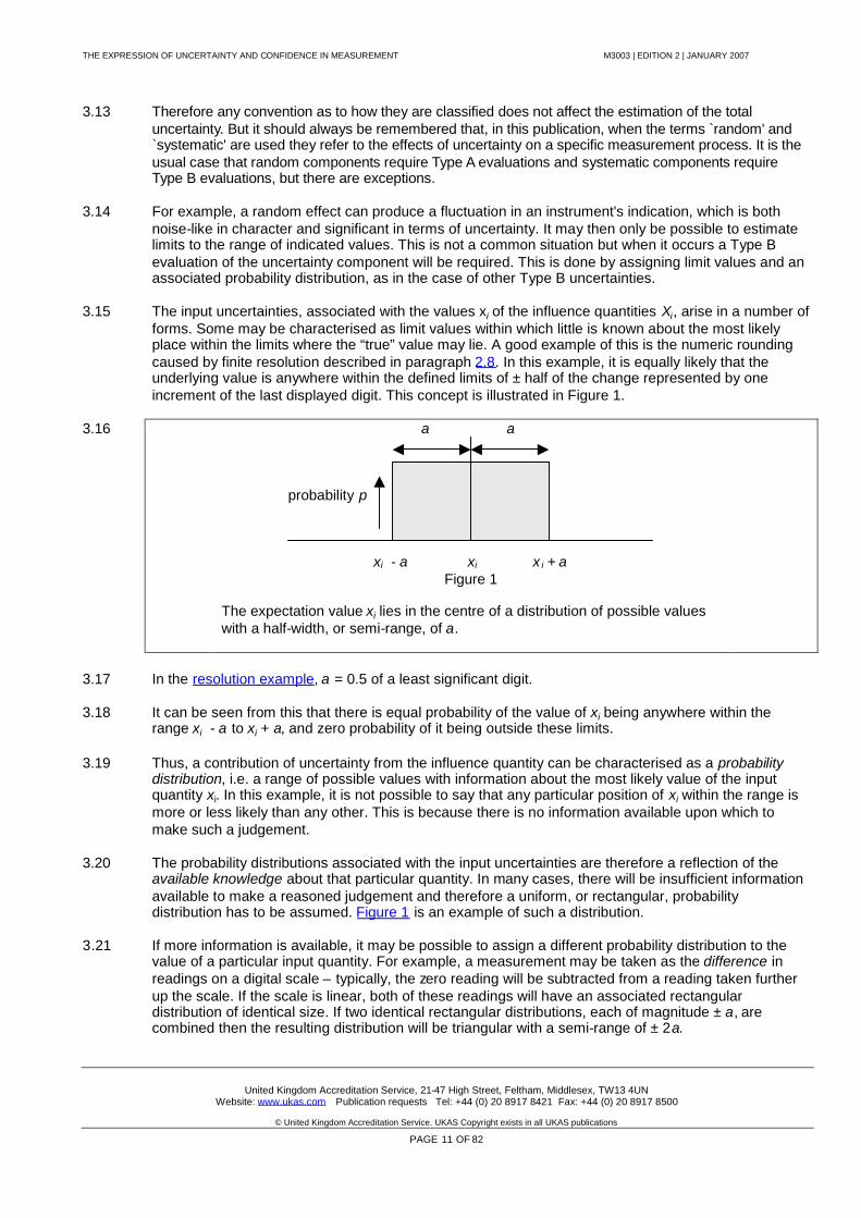
3.15 The input uncertainties, associated with the values xi of the influence quantities Xi, arise in a number offorms. Some may be characterised as limit values within which little is known about the most likelyplace within the limits where the “true” value may lie. A good example of this is the numeric roundingcaused by finite resolution described in paragraph 2.8. In this example, it is equally likely that theunderlying value is anywhere within the defined limits of ± half of the change represented by oneincrement of the last displayed digit. This concept is illustrated in Figure 1.
3.16 a a
probability p
xi - a xi x i + aFigure 1
The expectation value xi lies in the centre of a distribution of possible valueswith a half-width, or semi-range, of a.
3.17 In the resolution example, a = 0.5 of a least significant digit.
3.18 It can be seen from this that there is equal probability of the value of xi being anywhere within therange xi - a to xi + a, and zero probability of it being outside these limits.
3.19 Thus, a contribution of uncertainty from the influence quantity can be characterised as a probabilitydistribution, i.e. a range of possible values with information about the most likely value of the inputquantity xi. In this example, it is not possible to say that any particular position of xi within the range ismore or less likely than any other. This is because there is no information available upon which tomake such a judgement.
3.20 The probability distributions associated with the input uncertainties are therefore a reflection of theavailable knowledge about that particular quantity. In many cases, there will be insufficient informationavailable to make a reasoned judgement and therefore a uniform, or rectangular, probabilitydistribution has to be assumed. Figure 1 is an example of such a distribution.
3.21 If more information is available, it may be possible to assign a different probability distribution to thevalue of a particular input quantity. For example, a measurement may be taken as the difference inreadings on a digital scale – typically, the zero reading will be subtracted from a reading taken furtherup the scale. If the scale is linear, both of these readings will have an associated rectangulardistribution of identical size. If two identical rectangular distributions, each of magnitude ± a, arecombined then the resulting distribution will be triangular with a semi-range of ± 2a.

THE EXPRESSION OF UNCERTAINTY AND CONFIDENCE IN MEASUREMENT M3003 | EDITION 2 | JANUARY 2007
United Kingdom Accreditation Service, 21-47 High Street, Feltham, Middlesex, TW13 4UNWebsite: www.ukas.com Publication requests Tel: +44 (0) 20 8917 8421 Fax: +44 (0) 20 8917 8500
© United Kingdom Accreditation Service. UKAS Copyright exists in all UKAS publications
PAGE 12 OF 82
probability p
xi - 2a xi xi + 2a
Figure 2
Combination of two identical rectangular distributions, eachwith semi-range limits of ± a, yields a triangular distributionwith a semi-range of ± 2a.
3.22 There are other possible distributions that may be assigned. For example, when makingmeasurements of radio-frequency power an uncertainty arises due to imperfect matching between thesource and the termination. The imperfect match usually involves an unknown phase angle. Thismeans that a cosine function characterises the probability distribution for the uncertainty. Harris andWarner[3] have shown that a symmetrical U-shaped probability distribution arises from this effect. Inthis example, the distribution has been evaluated from a theoretical analysis of the principles involved.
xi - a xi xi + a
Figure 3
U-shaped distribution, associated with RF mismatch uncertainty. For thissituation, xi is likely to be close to one or other of the edges of thedistribution.
3.23 An evaluation of the effects of non-repeatability, performed by statistical methods, will usually yield aGaussian or normal distribution. Further details on this process can be found in Section 4.
THE EXPRESSION OF UNCERTAINTY AND CONFIDENCE IN MEASUREMENT M3003 | EDITION 2 | JANUARY 2007
United Kingdom Accreditation Service, 21-47 High Street, Feltham, Middlesex, TW13 4UNWebsite: www.ukas.com Publication requests Tel: +44 (0) 20 8917 8421 Fax: +44 (0) 20 8917 8500
© United Kingdom Accreditation Service. UKAS Copyright exists in all UKAS publications
PAGE 13 OF 82
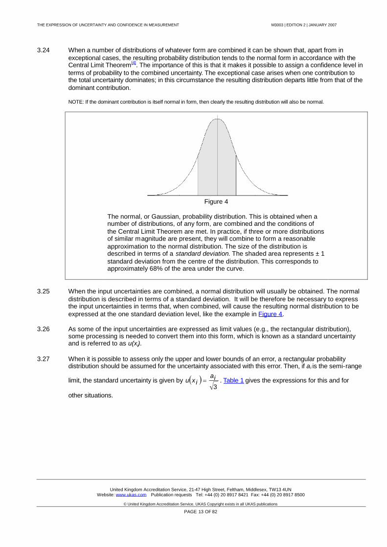
3.24 When a number of distributions of whatever form are combined it can be shown that, apart from inexceptional cases, the resulting probability distribution tends to the normal form in accordance with theCentral Limit Theorem[4]. The importance of this is that it makes it possible to assign a confidence level interms of probability to the combined uncertainty. The exceptional case arises when one contribution tothe total uncertainty dominates; in this circumstance the resulting distribution departs little from that of thedominant contribution.
NOTE: If the dominant contribution is itself normal in form, then clearly the resulting distribution will also be normal.
Figure 4
The normal, or Gaussian, probability distribution. This is obtained when anumber of distributions, of any form, are combined and the conditions ofthe Central Limit Theorem are met. In practice, if three or more distributionsof similar magnitude are present, they will combine to form a reasonableapproximation to the normal distribution. The size of the distribution isdescribed in terms of a standard deviation. The shaded area represents ± 1standard deviation from the centre of the distribution. This corresponds toapproximately 68% of the area under the curve.
3.25 When the input uncertainties are combined, a normal distribution will usually be obtained. The normaldistribution is described in terms of a standard deviation. It will be therefore be necessary to expressthe input uncertainties in terms that, when combined, will cause the resulting normal distribution to beexpressed at the one standard deviation level, like the example in Figure 4.
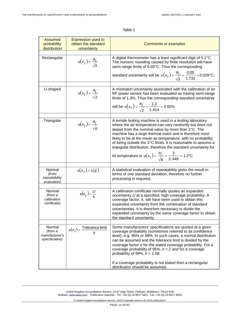
3.26 As some of the input uncertainties are expressed as limit values (e.g., the rectangular distribution),some processing is needed to convert them into this form, which is known as a standard uncertaintyand is referred to as u(xi).
3.27 When it is possible to assess only the upper and lower bounds of an error, a rectangular probabilitydistribution should be assumed for the uncertainty associated with this error. Then, if a i is the semi-range
limit, the standard uncertainty is given by 3ia
ixu . Table 1 gives the expressions for this and for
other situations.
THE EXPRESSION OF UNCERTAINTY AND CONFIDENCE IN MEASUREMENT M3003 | EDITION 2 | JANUARY 2007
United Kingdom Accreditation Service, 21-47 High Street, Feltham, Middlesex, TW13 4UNWebsite: www.ukas.com Publication requests Tel: +44 (0) 20 8917 8421 Fax: +44 (0) 20 8917 8500
© United Kingdom Accreditation Service. UKAS Copyright exists in all UKAS publications
PAGE 14 OF 82
Table 1
Assumedprobabilitydistribution
Expression used toobtain the standard
uncertaintyComments or examples
Rectangular
3ia
ixu A digital thermometer has a least significant digit of 0.1°C.The numeric rounding caused by finite resolution will havesemi-range limits of 0.05°C. Thus the corresponding
standard uncertainty will be 732.105.0
3ia
ixu 0.029°C.
U-shaped
2ia
ixu A mismatch uncertainty associated with the calibration of anRF power sensor has been evaluated as having semi-rangelimits of 1.3%. Thus the corresponding standard uncertainty
will be 414.13.1
2ia
ixu 0.92%
Triangular
6ia
ixu A tensile testing machine is used in a testing laboratorywhere the air temperature can vary randomly but does notdepart from the nominal value by more than 3°C. Themachine has a large thermal mass and is therefore mostlikely to be at the mean air temperature, with no probabilityof being outside the 3°C limits. It is reasonable to assume atriangular distribution, therefore the standard uncertainty for
its temperature is 449.23
6ia
ixu 1.2°C
Normal(from
repeatabilityevaluation)
qsixu A statistical evaluation of repeatability gives the result interms of one standard deviation; therefore no furtherprocessing is required.
Normal(from a
calibrationcertificate)
kU
ixu A calibration certificate normally quotes an expandeduncertainty U at a specified, high coverage probability. Acoverage factor, k, will have been used to obtain thisexpanded uncertainty from the combination of standarduncertainties. It is therefore necessary to divide theexpanded uncertainty by the same coverage factor to obtainthe standard uncertainty.
Normal(from a
manufacturer’sspecification)
kixu limitTolerance
Some manufacturers’ specifications are quoted at a givencoverage probability (sometimes referred to as confidencelevel), e.g. 95% or 99%. In such cases, a normal distributioncan be assumed and the tolerance limit is divided by thecoverage factor k for the stated coverage probability. For acoverage probability of 95%, k = 2 and for a coverageprobability of 99%, k = 2.58.
If a coverage probability is not stated then a rectangulardistribution should be assumed.
THE EXPRESSION OF UNCERTAINTY AND CONFIDENCE IN MEASUREMENT M3003 | EDITION 2 | JANUARY 2007
United Kingdom Accreditation Service, 21-47 High Street, Feltham, Middlesex, TW13 4UNWebsite: www.ukas.com Publication requests Tel: +44 (0) 20 8917 8421 Fax: +44 (0) 20 8917 8500
© United Kingdom Accreditation Service. UKAS Copyright exists in all UKAS publications
PAGE 15 OF 82
3.28 The quantities Xi that affect the measurand Y may not have a direct, one to one, relationship with it.Indeed, they may be entirely different units altogether. For example, a dimensional laboratory may usesteel gauge blocks for calibration of measuring tools. A significant influence quantity is temperature.Because the gauge blocks have a significant temperature coefficient of expansion, there is anuncertainty that arises in their length due to an uncertainty in temperature units.
3.29 In order to translate the temperature uncertainty into an uncertainty in length units, it is necessary toknow how sensitive the length of the gauge block is to temperature. In other words, a sensitivitycoefficient is required.
3.30 The sensitivity coefficient simply describes how sensitive the result is to a particular influence quantity.In this example, the steel used in the manufacture of gauge blocks has a temperature coefficient ofexpansion of approximately +11.5 x 10⁻⁶ per °C. So, in this case, this figure can be used as thesensitivity coefficient.
The sensitivity coefficient associated with each input estimate x i is referred to as ci . It is the partialderivative of the model function f with respect to Xi, evaluated at the input estimates xi. It is given by
3.31
In other words, it describes how the output estimate y varies with a corresponding small change in aninput estimate xi.
3.32 The calculations required to obtain sensitivity coefficients by partial differentiation can be a lengthyprocess, particularly when there are many input contributions and uncertainty estimates are needed for arange of values. If the functional relationship is not known for a particular measurement system thesensitivity coefficients can sometimes be obtained by the practical approach of changing one of the inputvariables by a known amount, while keeping all other inputs constant, and noting the change in theoutput estimate. This approach can also be used if f is known but the determination of the partialderivatives is likely to be difficult.
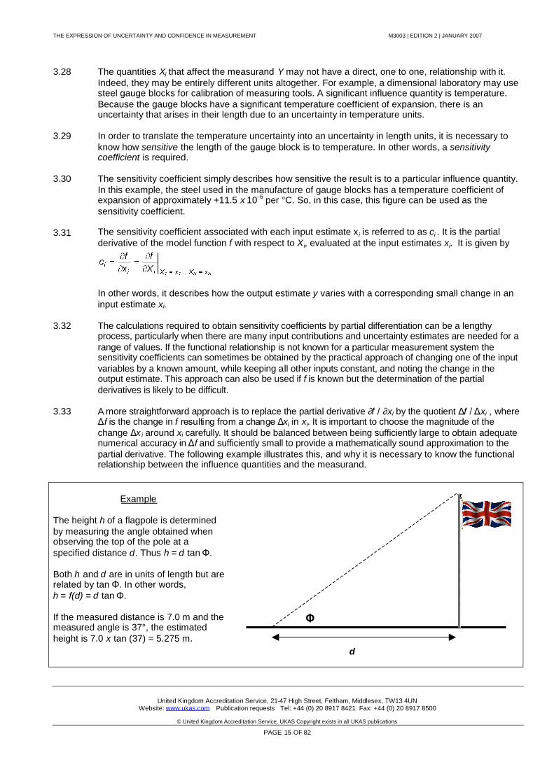
3.33 A more straightforward approach is to replace the partial derivative ∂f / ∂xi by the quotient Δf / Δxi , whereΔf is the change in f resulting from a change Δxi in xi. It is important to choose the magnitude of thechange Δx i around xi carefully. It should be balanced between being sufficiently large to obtain adequatenumerical accuracy in Δf and sufficiently small to provide a mathematically sound approximation to thepartial derivative. The following example illustrates this, and why it is necessary to know the functionalrelationship between the influence quantities and the measurand.
Example
The height h of a flagpole is determinedby measuring the angle obtained whenobserving the top of the pole at aspecified distance d. Thus h = d tanΦ.
Both h and d are in units of length but arerelated by tan Φ. In other words,h = f(d) = d tanΦ.
If the measured distance is 7.0 m and themeasured angle is 37°, the estimatedheight is 7.0 x tan (37) = 5.275 m.
Φ
d
THE EXPRESSION OF UNCERTAINTY AND CONFIDENCE IN MEASUREMENT M3003 | EDITION 2 | JANUARY 2007
United Kingdom Accreditation Service, 21-47 High Street, Feltham, Middlesex, TW13 4UNWebsite: www.ukas.com Publication requests Tel: +44 (0) 20 8917 8421 Fax: +44 (0) 20 8917 8500
© United Kingdom Accreditation Service. UKAS Copyright exists in all UKAS publications
PAGE 16 OF 82
3.34 If the uncertainty in d is, say, ± 0.1 m then the estimate of h could be anywhere between(7.0 – 0.1) tan (37) and (7.0 + 0.1) tan (37), i.e. between 5.200 m and 5.350 m. A change of ± 0.1 m inthe input quantity x i has resulted in a change of ± 0.075 m in the output estimate y. The sensitivity
coefficient is therefore 75.01.0
075.0 .
3.35 Similar reasoning can be applied to the uncertainty in the angleΦ. If the uncertainty in Φ is ± 0.5°,then the estimate of h could be anywhere between 7.0 tan (36.5) and 7.0 tan (37.5), i.e. between5.179 m and 5.371 m. A change of ± 0.5° in the input quantity xi has resulted in a change of ± 0.096 m
in the output estimate y. The sensitivity coefficient is therefore 192.05.0
096.0 metre per degree.
3.36 Once the standard uncertainties xi and the sensitivity coefficients ci have been evaluated, theuncertainties have to be combined in order to give a single value of uncertainty to be associated withthe estimate y of the measurand Y. This is known as the combined standard uncertainty and is giventhe symbol uc(y).
3.37 The combined standard uncertainty is calculated as follows:
3.38
N
ii
N
iiic yuxucyu
1
2
1
22 (1)
3.39 In other words, the individual standard uncertainties, expressed in terms of the measurand, aresquared; these squared values are added and the square root is taken.
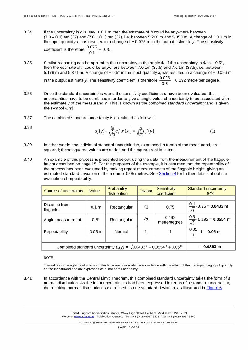
3.40 An example of this process is presented below, using the data from the measurement of the flagpoleheight described on page 15. For the purposes of the example, it is assumed that the repeatability ofthe process has been evaluated by making repeat measurements of the flagpole height, giving anestimated standard deviation of the mean of 0.05 metres. See Section 4 for further details about theevaluation of repeatability.
Source of uncertainty Value Probabilitydistribution Divisor Sensitivity
coefficientStandard uncertainty
ui(y)
Distance fromflagpole 0.1 m Rectangular √3 0.75 75.0
3
1.0 = 0.0433 m
Angle measurement 0.5° Rectangular √3 0.192metre/degree
192.035.0 = 0.0554 m
Repeatability 0.05 m Normal 1 1 1105.0 = 0.05 m
Combined standard uncertainty uc(y) = 222 05.00554.00433.0 = 0.0863 m
NOTE
The values in the right-hand column of the table are now scaled in accordance with the effect of the corresponding input quantityon the measurand and are expressed as a standard uncertainty.
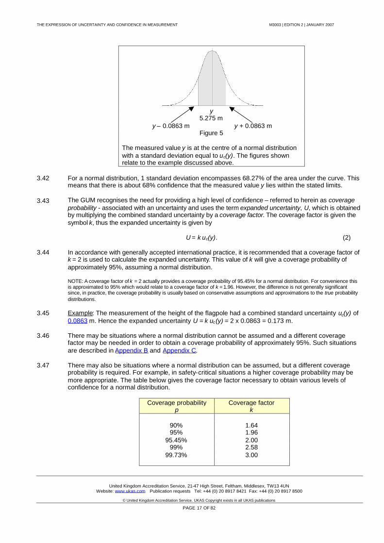
3.41 In accordance with the Central Limit Theorem, this combined standard uncertainty takes the form of anormal distribution. As the input uncertainties had been expressed in terms of a standard uncertainty,the resulting normal distribution is expressed as one standard deviation, as illustrated in Figure 5.
THE EXPRESSION OF UNCERTAINTY AND CONFIDENCE IN MEASUREMENT M3003 | EDITION 2 | JANUARY 2007
United Kingdom Accreditation Service, 21-47 High Street, Feltham, Middlesex, TW13 4UNWebsite: www.ukas.com Publication requests Tel: +44 (0) 20 8917 8421 Fax: +44 (0) 20 8917 8500
© United Kingdom Accreditation Service. UKAS Copyright exists in all UKAS publications
PAGE 17 OF 82
y5.275 m
y – 0.0863 m y + 0.0863 mFigure 5
The measured value y is at the centre of a normal distributionwith a standard deviation equal to uc(y). The figures shownrelate to the example discussed above.
3.42 For a normal distribution, 1 standard deviation encompasses 68.27% of the area under the curve. Thismeans that there is about 68% confidence that the measured value y lies within the stated limits.
3.43 The GUM recognises the need for providing a high level of confidence – referred to herein as coverageprobability - associated with an uncertainty and uses the term expanded uncertainty, U, which is obtainedby multiplying the combined standard uncertainty by a coverage factor. The coverage factor is given thesymbol k, thus the expanded uncertainty is given by
U = k uc(y). (2)
3.44 In accordance with generally accepted international practice, it is recommended that a coverage factor ofk = 2 is used to calculate the expanded uncertainty. This value of k will give a coverage probability ofapproximately 95%, assuming a normal distribution.
NOTE: A coverage factor of k = 2 actually provides a coverage probability of 95.45% for a normal distribution. For convenience thisis approximated to 95% which would relate to a coverage factor of k = 1.96. However, the difference is not generally significantsince, in practice, the coverage probability is usually based on conservative assumptions and approximations to the true probabilitydistributions.
3.45 Example: The measurement of the height of the flagpole had a combined standard uncertainty uc(y) of0.0863 m. Hence the expanded uncertainty U = k uc(y) = 2 x 0.0863 = 0.173 m.
3.46 There may be situations where a normal distribution cannot be assumed and a different coveragefactor may be needed in order to obtain a coverage probability of approximately 95%. Such situationsare described in Appendix B and Appendix C.
3.47 There may also be situations where a normal distribution can be assumed, but a different coverageprobability is required. For example, in safety-critical situations a higher coverage probability may bemore appropriate. The table below gives the coverage factor necessary to obtain various levels ofconfidence for a normal distribution.
Coverage probability Coverage factorp k
90% 1.6495% 1.96
95.45% 2.0099% 2.58
99.73% 3.00
THE EXPRESSION OF UNCERTAINTY AND CONFIDENCE IN MEASUREMENT M3003 | EDITION 2 | JANUARY 2007
United Kingdom Accreditation Service, 21-47 High Street, Feltham, Middlesex, TW13 4UNWebsite: www.ukas.com Publication requests Tel: +44 (0) 20 8917 8421 Fax: +44 (0) 20 8917 8500
© United Kingdom Accreditation Service. UKAS Copyright exists in all UKAS publications
PAGE 18 OF 82
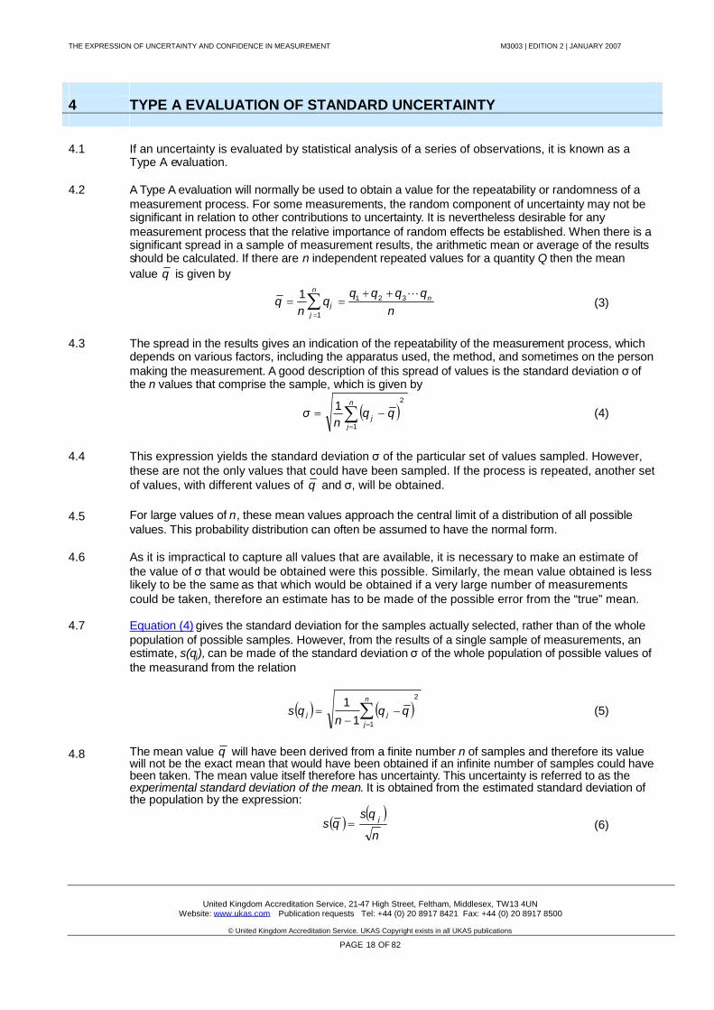
4 TYPE A EVALUATION OF STANDARD UNCERTAINTY
4.1 If an uncertainty is evaluated by statistical analysis of a series of observations, it is known as aType A evaluation.
4.2 A Type A evaluation will normally be used to obtain a value for the repeatability or randomness of ameasurement process. For some measurements, the random component of uncertainty may not besignificant in relation to other contributions to uncertainty. It is nevertheless desirable for anymeasurement process that the relative importance of random effects be established. When there is asignificant spread in a sample of measurement results, the arithmetic mean or average of the resultsshould be calculated. If there are n independent repeated values for a quantity Q then the meanvalue q is given by
nqqqq
qn
q nn
jj
321
1
1
(3)
4.3 The spread in the results gives an indication of the repeatability of the measurement process, whichdepends on various factors, including the apparatus used, the method, and sometimes on the personmaking the measurement. A good description of this spread of values is the standard deviation σofthe n values that comprise the sample, which is given by
2
1
1
n
jj qq
nσ (4)
4.4 This expression yields the standard deviation σof the particular set of values sampled. However,these are not the only values that could have been sampled. If the process is repeated, another setof values, with different values of q and σ, will be obtained.
4.5 For large values of n, these mean values approach the central limit of a distribution of all possiblevalues. This probability distribution can often be assumed to have the normal form.
4.6 As it is impractical to capture all values that are available, it is necessary to make an estimate ofthe value of σthat would be obtained were this possible. Similarly, the mean value obtained is lesslikely to be the same as that which would be obtained if a very large number of measurementscould be taken, therefore an estimate has to be made of the possible error from the “true” mean.
4.7 Equation (4) gives the standard deviation for the samples actually selected, rather than of the wholepopulation of possible samples. However, from the results of a single sample of measurements, anestimate, s(qj), can be made of the standard deviationσof the whole population of possible values ofthe measurand from the relation
2
111
n
jjj qq
nqs (5)
4.8 The mean value q will have been derived from a finite number n of samples and therefore its valuewill not be the exact mean that would have been obtained if an infinite number of samples could havebeen taken. The mean value itself therefore has uncertainty. This uncertainty is referred to as theexperimental standard deviation of the mean. It is obtained from the estimated standard deviation ofthe population by the expression:
n
qsqs j (6)
THE EXPRESSION OF UNCERTAINTY AND CONFIDENCE IN MEASUREMENT M3003 | EDITION 2 | JANUARY 2007
United Kingdom Accreditation Service, 21-47 High Street, Feltham, Middlesex, TW13 4UNWebsite: www.ukas.com Publication requests Tel: +44 (0) 20 8917 8421 Fax: +44 (0) 20 8917 8500
© United Kingdom Accreditation Service. UKAS Copyright exists in all UKAS publications
PAGE 19 OF 82
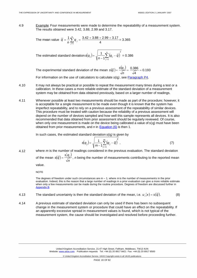
4.9 Example: Four measurements were made to determine the repeatability of a measurement system.The results obtained were 3.42, 3.88, 2.99 and 3.17.
The mean value4
17.399.288.342.31
1
n
jjq
nq = 3.365
The estimated standard deviation 2
111
n
jjj qq
nqs = 0.386
The experimental standard deviation of the mean 193.0
4386.0
n
qsqs j
For information on the use of calculators to calculate s(qj), see Paragraph P4.
4.10 It may not always be practical or possible to repeat the measurement many times during a test or acalibration. In these cases a more reliable estimate of the standard deviation of a measurementsystem may be obtained from data obtained previously, based on a larger number of readings.
4.11 Whenever possible at least two measurements should be made as part of the procedure; however, itis acceptable for a single measurement to be made even though it is known that the system hasimperfect repeatability, and to rely on a previous assessment of the repeatability of similar devices.This procedure must be treated with caution because the reliability of a previous assessment willdepend on the number of devices sampled and how well this sample represents all devices. It is alsorecommended that data obtained from prior assessment should be regularly reviewed. Of course,when only one measurement is made on the device being calibrated a value of s(qj) must have beenobtained from prior measurements, and n in Equation (6) is then 1.
In such cases, the estimated standard deviation s(qj) is given by
2
111
m
jjj qq
mqs , (7)
4.12 where m is the number of readings considered in the previous evaluation. The standard deviation
of the mean n
qsqs j , n being the number of measurements contributing to the reported mean
value.
NOTE
The degrees of freedom under such circumstances are m – 1, where m is the number of measurements in the priorevaluation. Indeed, this is the reason that a large number of readings in a prior evaluation can give a more reliable estimatewhen only a few measurements can be made during the routine procedure. Degrees of freedom are discussed further inAppendix B.
4.13 The standard uncertainty is then the standard deviation of the mean, i.e. qsxu i . (8)
4.14 A previous estimate of standard deviation can only be used if there has been no subsequentchange in the measurement system or procedure that could have an effect on the repeatability. Ifan apparently excessive spread in measurement values is found, which is not typical of themeasurement system, the cause should be investigated and resolved before proceeding further.

THE EXPRESSION OF UNCERTAINTY AND CONFIDENCE IN MEASUREMENT M3003 | EDITION 2 | JANUARY 2007
United Kingdom Accreditation Service, 21-47 High Street, Feltham, Middlesex, TW13 4UNWebsite: www.ukas.com Publication requests Tel: +44 (0) 20 8917 8421 Fax: +44 (0) 20 8917 8500
© United Kingdom Accreditation Service. UKAS Copyright exists in all UKAS publications
PAGE 20 OF 82
5 TYPE B EVALUATION OF STANDARD UNCERTAINTY
5.1 It is probable that systematic components of uncertainty, i.e. those that account for errors that remainconstant while the measurement is made, will be estimated from Type B evaluations. The mostimportant of these systematic components, for a reference instrument, will often be the importeduncertainties associated with its own calibration. However, there can be, and usually are, otherimportant contributions to systematic errors in measurement that arise in the equipment user's ownlaboratory.
5.2 The successful identification and evaluation of these contributions depends on a detailed knowledgeof the measurement process and the experience of the person making the measurements. The needfor the utmost vigilance in preventing mistakes cannot be overemphasised. Common examples areerrors in the corrections applied to values, transcription errors, and faults in software designed tocontrol or report on a measurement process. The effects of such mistakes cannot readily be includedin the evaluation of uncertainty.
5.3 In evaluating the components of uncertainty it is necessary to consider and include at least thefollowing possible sources:
(a) The reported calibration uncertainty assigned to reference standards and any drift or instability in theirvalues or readings.
(b) The calibration of measuring equipment, including ancillaries such as connecting leads etc., and anydrift or instability in their values or readings.
(c) The equipment or item being measured, for example its resolution and any instability during themeasurement. It should be noted that the anticipated long-term performance of the item beingcalibrated is not normally included in the uncertainty evaluation for that calibration.
(d) The operational procedure.
(e) Variability between different staff carrying out the same type of measurement.
(f) The effects of environmental conditions on any or all of the above.
5.4 Whenever possible, corrections should be made for errors revealed by calibration or other sources;the convention is that an error is given a positive sign if the measured value is greater than theconventional true value. The correction for error involves subtracting the error from the measuredvalue. On occasions, to simplify the measurement process it may be convenient to treat such anerror, when it is small compared with other uncertainties, as if it were a systematic uncertainty equalto (±) the uncorrected error magnitude.
5.5 Having identified all the possible systematic components of uncertainty based as far as possible onexperimental data or on theoretical grounds, they should be characterised in terms of standarduncertainties based on the assessed probability distributions. The probability distribution of anuncertainty obtained from a Type B evaluation can take a variety of forms but it is generallyacceptable to assign well-defined geometric shapes for which the standard uncertainty can beobtained from a simple calculation. These distributions and sample calculations are presented indetail in paragraphs 3.15 to 3.22.

THE EXPRESSION OF UNCERTAINTY AND CONFIDENCE IN MEASUREMENT M3003 | EDITION 2 | JANUARY 2007
United Kingdom Accreditation Service, 21-47 High Street, Feltham, Middlesex, TW13 4UNWebsite: www.ukas.com Publication requests Tel: +44 (0) 20 8917 8421 Fax: +44 (0) 20 8917 8500
© United Kingdom Accreditation Service. UKAS Copyright exists in all UKAS publications
PAGE 21 OF 82
6 REPORTING OF RESULTS
6.1 After the expanded uncertainty has been calculated for a coverage probability of 95% the value ofthe measurand and expanded uncertainty should be reported as y ± U and accompanied by thefollowing statement of confidence:
6.2 "The reported expanded uncertainty is based on a standard uncertainty multiplied by a coveragefactor k = 2, providing a coverage probability of approximately 95%. The uncertainty evaluation hasbeen carried out in accordance with UKAS requirements".
6.3 In cases where the procedure of Appendix B has been followed the actual value of the coveragefactor should be substituted for k = 2 and the following statement used:
6.4 "The reported expanded uncertainty is based on a standard uncertainty multiplied by a coveragefactor k = XX, which for a t-distribution with veff = YY effective degrees of freedom corresponds to acoverage probability of approximately 95%. The uncertainty evaluation has been carried out inaccordance with UKAS requirements".
6.5 For the purposes of this document "approximately" is interpreted as meaning sufficiently close thatany difference may be considered insignificant.
6.6 In the special circumstances where a dominant non-Gaussian Type B contribution occurs refer toAppendix C. If uncertainty is being reported as an analytical expression, refer to Appendix L .
6.7 Uncertainties are usually expressed in bilateral terms (±) either in units of the measurand or asrelative values, for example as a percentage (%), parts per million (ppm), 1 in 10X, etc. However theremay be situations where the upper and lower uncertainty values are different; for example if cosineerrors are involved. If such differences are small then the most practical approach is to report theexpanded uncertainty as ± the larger of the two. However if there is a significant difference betweenthe upper and lower values then they should be evaluated and reported separately.
6.8 The number of figures in a reported uncertainty should always reflect practical measurementcapability. In view of the process for estimating uncertainties it is seldom justified to report more thantwo significant figures. It is therefore recommended that the expanded uncertainty be rounded to twosignificant figures, using the normal rules of rounding. The numerical value of the measurement resultshould in the final statement normally be rounded to the least significant figure in the value of theexpanded uncertainty assigned to the measurement result.
6.9 Rounding should always be carried out at the end of the process in order to avoid the effects ofcumulative rounding errors.
THE EXPRESSION OF UNCERTAINTY AND CONFIDENCE IN MEASUREMENT M3003 | EDITION 2 | JANUARY 2007
United Kingdom Accreditation Service, 21-47 High Street, Feltham, Middlesex, TW13 4UNWebsite: www.ukas.com Publication requests Tel: +44 (0) 20 8917 8421 Fax: +44 (0) 20 8917 8500
© United Kingdom Accreditation Service. UKAS Copyright exists in all UKAS publications
PAGE 22 OF 82
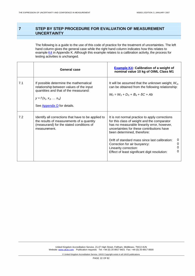
7 STEP BY STEP PROCEDURE FOR EVALUATION OF MEASUREMENTUNCERTAINTY
The following is a guide to the use of this code of practice for the treatment of uncertainties. The lefthand column gives the general case while the right hand column indicates how this relates toexample K4 in Appendix K. Although this example relates to a calibration activity, the process fortesting activities is unchanged.
General case Example K4: Calibration of a weight ofnominal value 10 kg of OIML Class M1
7.1 If possible determine the mathematicalrelationship between values of the inputquantities and that of the measurand:
y = f (x1, x2, … xN)
See Appendix D for details.
It will be assumed that the unknown weight, WX,can be obtained from the following relationship:
WX = WS + DS + δId + δC + Ab
7.2 Identify all corrections that have to be applied tothe results of measurements of a quantity(measurand) for the stated conditions ofmeasurement.
It is not normal practice to apply correctionsfor this class of weight and the comparatorhas no measurable linearity error, however,uncertainties for these contributions havebeen determined, therefore:
Drift of standard mass since last calibration:Correction for air buoyancy:Linearity correction:Effect of least significant digit resolution:
0000
THE EXPRESSION OF UNCERTAINTY AND CONFIDENCE IN MEASUREMENT M3003 | EDITION 2 | JANUARY 2007
United Kingdom Accreditation Service, 21-47 High Street, Feltham, Middlesex, TW13 4UNWebsite: www.ukas.com Publication requests Tel: +44 (0) 20 8917 8421 Fax: +44 (0) 20 8917 8500
© United Kingdom Accreditation Service. UKAS Copyright exists in all UKAS publications
PAGE 23 OF 82
General case Example K4: Calibration of a weight ofnominal value 10 kg of OIML Class M1
Source of uncertainty Limit(mg)
Distribution
WSCalibration of std. mass 30 Normal (k = 2)
DSDrift of standard mass 30 Rectangular
δCComparator linearity 3 Rectangular
δAbAir buoyancy 10 Rectangular
δIdResolution effects 10 Triangular
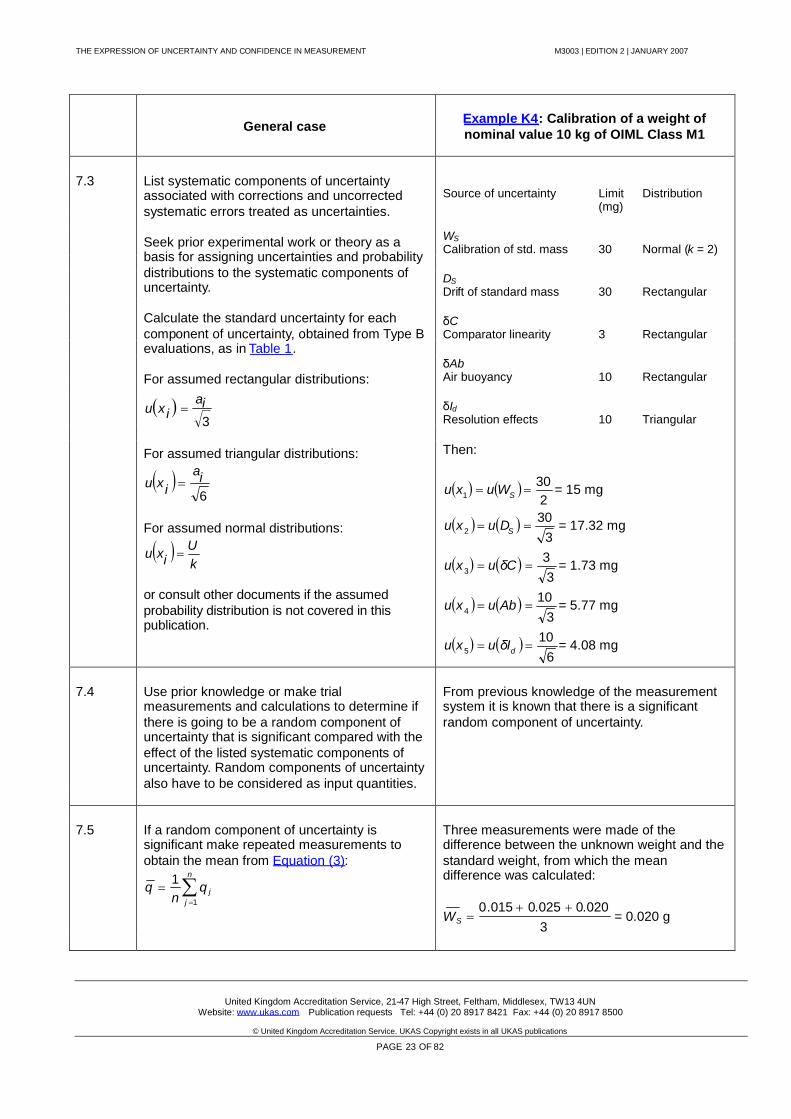
7.3 List systematic components of uncertaintyassociated with corrections and uncorrectedsystematic errors treated as uncertainties.
Seek prior experimental work or theory as abasis for assigning uncertainties and probabilitydistributions to the systematic components ofuncertainty.
Calculate the standard uncertainty for eachcomponent of uncertainty, obtained from Type Bevaluations, as in Table 1.
For assumed rectangular distributions:
3ia
ixu
For assumed triangular distributions:
6ia
ixu
For assumed normal distributions:
kU
ixu
or consult other documents if the assumedprobability distribution is not covered in thispublication.
Then:
2
301 SWuxu = 15 mg
3
302 SDuxu = 17.32 mg
3
33 Cuxu δ = 1.73 mg
3
104 Abuxu = 5.77 mg
6
105 dIuxu δ = 4.08 mg
7.4 Use prior knowledge or make trialmeasurements and calculations to determine ifthere is going to be a random component ofuncertainty that is significant compared with theeffect of the listed systematic components ofuncertainty. Random components of uncertaintyalso have to be considered as input quantities.
From previous knowledge of the measurementsystem it is known that there is a significantrandom component of uncertainty.
7.5 If a random component of uncertainty issignificant make repeated measurements toobtain the mean from Equation (3):
n
jjq
nq
1
1
Three measurements were made of thedifference between the unknown weight and thestandard weight, from which the meandifference was calculated:
3020.0025.0015.0
SW = 0.020 g
THE EXPRESSION OF UNCERTAINTY AND CONFIDENCE IN MEASUREMENT M3003 | EDITION 2 | JANUARY 2007
United Kingdom Accreditation Service, 21-47 High Street, Feltham, Middlesex, TW13 4UNWebsite: www.ukas.com Publication requests Tel: +44 (0) 20 8917 8421 Fax: +44 (0) 20 8917 8500
© United Kingdom Accreditation Service. UKAS Copyright exists in all UKAS publications
PAGE 24 OF 82
General case Example K4: Calibration of a weight ofnominal value 10 kg of OIML Class M1
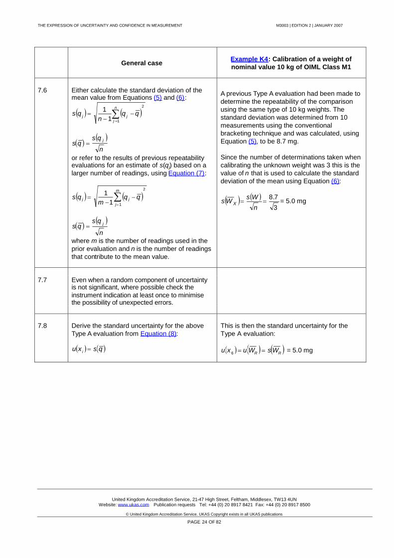
7.6 Either calculate the standard deviation of themean value from Equations (5) and (6):
2
111
n
jjj qq
nqs
n
qsqs j
or refer to the results of previous repeatabilityevaluations for an estimate of s(q j) based on alarger number of readings, using Equation (7):
2
111
m
jjj qq
mqs
n
qsqs j
where m is the number of readings used in theprior evaluation and n is the number of readingsthat contribute to the mean value.
A previous Type A evaluation had been made todetermine the repeatability of the comparisonusing the same type of 10 kg weights. Thestandard deviation was determined from 10measurements using the conventionalbracketing technique and was calculated, usingEquation (5), to be 8.7 mg.
Since the number of determinations taken whencalibrating the unknown weight was 3 this is thevalue of n that is used to calculate the standarddeviation of the mean using Equation (6):
3
7.8n
WsWs X = 5.0 mg
7.7 Even when a random component of uncertaintyis not significant, where possible check theinstrument indication at least once to minimisethe possibility of unexpected errors.
7.8 Derive the standard uncertainty for the aboveType A evaluation from Equation (8):
qsxu i
This is then the standard uncertainty for theType A evaluation:
RR WsWuxu 6 = 5.0 mg
THE EXPRESSION OF UNCERTAINTY AND CONFIDENCE IN MEASUREMENT M3003 | EDITION 2 | JANUARY 2007
United Kingdom Accreditation Service, 21-47 High Street, Feltham, Middlesex, TW13 4UNWebsite: www.ukas.com Publication requests Tel: +44 (0) 20 8917 8421 Fax: +44 (0) 20 8917 8500
© United Kingdom Accreditation Service. UKAS Copyright exists in all UKAS publications
PAGE 25 OF 82
General case Example K4: Calibration of a weight ofnominal value 10 kg of OIML Class M1
7.9 Calculate the combined standard uncertainty foruncorrelated input quantities using Equation (1) ifabsolute values are used:
N
ii
N
iiic yuxucyu
1
2
1
22 , where ci is the
partial derivative ixf , or a known sensitivitycoefficient.
Alternatively use Equation (11) if the standarduncertainties are relative values:
N
i i
iic
xxup
yyu
1
2
, where p i are known
positive or negative exponents in the functionalrelationship.
The units of all standard uncertainties are interms of those of the measurand, i.e. milligrams,and the functional relationship between theinput quantities and the measurand is a linearsummation; therefore all the sensitivitycoefficients are unity (c i =1).
7.10 If correlation is suspected use the guidance inparagraph D3 or consult other referenceddocuments.
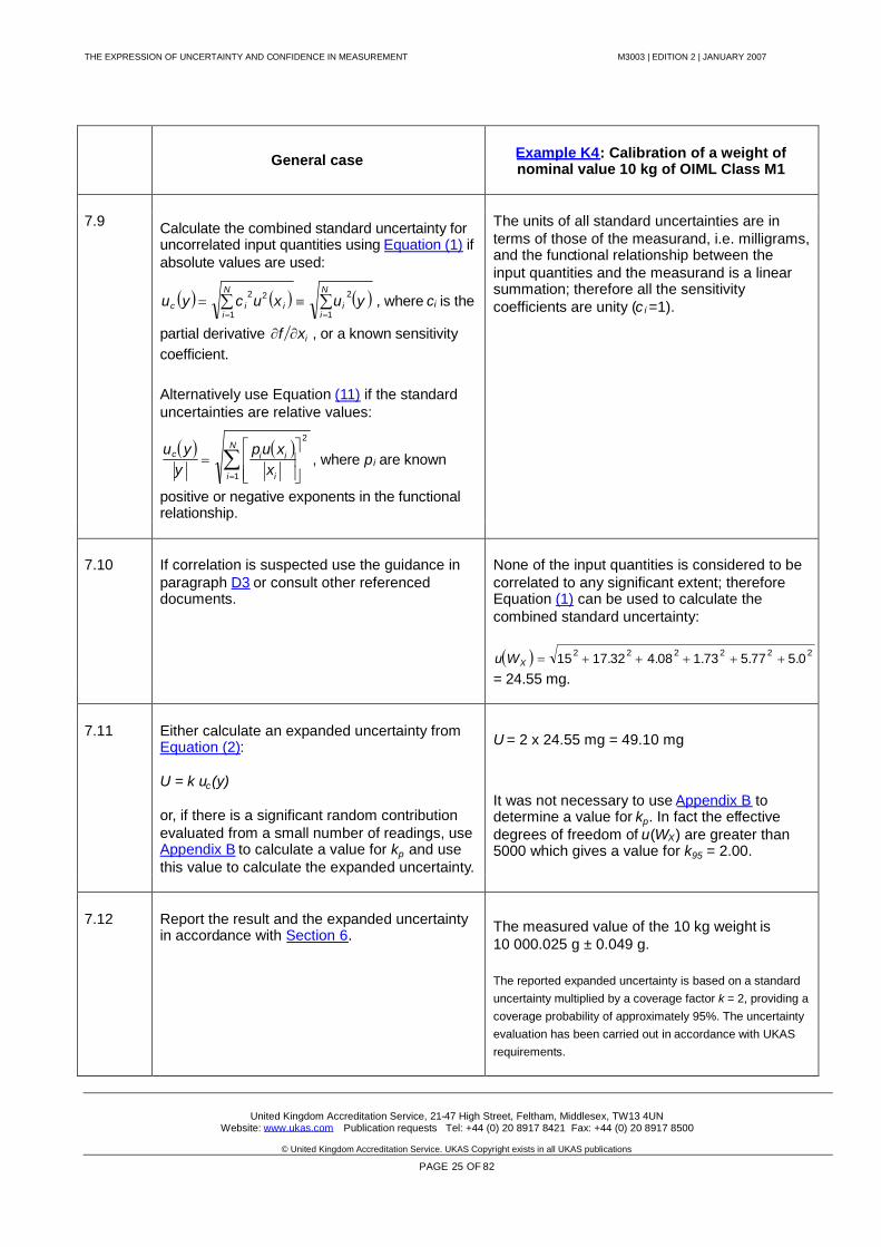
None of the input quantities is considered to becorrelated to any significant extent; thereforeEquation (1) can be used to calculate thecombined standard uncertainty:
222222 0.577.573.108.432.1715 XWu
= 24.55 mg.
7.11 Either calculate an expanded uncertainty fromEquation (2):
U = k·uc(y)
or, if there is a significant random contributionevaluated from a small number of readings, useAppendix B to calculate a value for kp and usethis value to calculate the expanded uncertainty.
U = 2 x 24.55 mg = 49.10 mg
It was not necessary to use Appendix B todetermine a value for kp. In fact the effectivedegrees of freedom of u(WX) are greater than5000 which gives a value for k95 = 2.00.
7.12 Report the result and the expanded uncertaintyin accordance with Section 6. The measured value of the 10 kg weight is
10 000.025 g ± 0.049 g.
The reported expanded uncertainty is based on a standarduncertainty multiplied by a coverage factor k = 2, providing acoverage probability of approximately 95%. The uncertaintyevaluation has been carried out in accordance with UKASrequirements.
THE EXPRESSION OF UNCERTAINTY AND CONFIDENCE IN MEASUREMENT M3003 | EDITION 2 | JANUARY 2007
United Kingdom Accreditation Service, 21-47 High Street, Feltham, Middlesex, TW13 4UNWebsite: www.ukas.com Publication requests Tel: +44 (0) 20 8917 8421 Fax: +44 (0) 20 8917 8500
© United Kingdom Accreditation Service. UKAS Copyright exists in all UKAS publications
PAGE 26 OF 82
APPENDIX ABEST MEASUREMENT CAPABILITY
A1 Best measurement capability (BMC) is a term normally used to describe the uncertainty that appearsin an accredited calibration laboratory's schedule of accreditation and is the uncertainty for which thelaboratory has been accredited using the procedure that was the subject of assessment. The bestmeasurement capability should be calculated according to the procedures given in this document andshould normally be quoted as an expanded uncertainty at a coverage probability of 95%, whichusually requires the use of a coverage factor of k = 2.
A2 An accredited laboratory is not permitted to report an uncertainty smaller than their accredited bestmeasurement capability but may report an equal or larger uncertainty. Since the magnitude of theuncertainty reported on a certificate of calibration will often depend on properties of the device beingcalibrated any definition of best measurement capability should not include uncertainties that aredependent on this device. However, no device is perfect and so the concept of “nearly ideal” is usedin association with the evaluation of a BMC. It may also be the case that an accredited laboratory canachieve a particular uncertainty if conditions are optimum but cannot achieve this uncertaintyroutinely.
A3 In order to promote harmony between accredited laboratories and between accreditation bodies theEA has adopted the following definition of best measurement capability:
The smallest uncertainty of measurement a laboratory can achieve within its scope of accreditation,when performing more or less routine calibrations of nearly ideal measurement standards intended todefine, realize, conserve or reproduce a unit of that quantity or one or more of its values, or whenperforming more or less routine calibrations of nearly ideal measuring instruments designed for themeasurement of that quantity.
In other words "best measurement capability" is the smallest uncertainty a laboratory can achievewhen performing more or less routine calibrations on a nearly ideal device being calibrated.
A4 A nearly ideal device is one that is available but does not necessarily represent the majority ofdevices that the laboratory may be asked to calibrate. The properties of these devices that areconsidered to be nearly ideal will depend on the field of calibration but may include an instrument withvery low random fluctuations, negligible temperature coefficient, very low voltage reflection coefficientetc. The uncertainty budget that is intended to demonstrate the best measurement uncertainty shouldstill include contributions from the properties of the device being calibrated that are considered to benearly ideal but the value of the uncertainty may be entered as zero or a negligible value, if this is thecase. Where necessary the laboratory's schedule of accreditation will include a remark that describesthe conditions under which the best measurement capability can be achieved.
A5 By "more or less routine calibrations" it is meant that the laboratory shall be able to achieve the statedcapability in the normal work that it performs under its accreditation and, by implication, using theprocedures, equipment and facilities that were the subject of the assessment. Where a smalleruncertainty can be achieved by, for example, taking a large number of readings this should beconsidered when arriving at the budget for the best measurement capability and would therefore bewithin the "more or less routine" conditions.
THE EXPRESSION OF UNCERTAINTY AND CONFIDENCE IN MEASUREMENT M3003 | EDITION 2 | JANUARY 2007
United Kingdom Accreditation Service, 21-47 High Street, Feltham, Middlesex, TW13 4UNWebsite: www.ukas.com Publication requests Tel: +44 (0) 20 8917 8421 Fax: +44 (0) 20 8917 8500
© United Kingdom Accreditation Service. UKAS Copyright exists in all UKAS publications
PAGE 27 OF 82
A6 It is sometimes the case that a laboratory may wish to be accredited for a measurement uncertaintythat is larger than it can actually achieve. If the principles of this document are followed whenconstructing the uncertainty budget the resulting expanded uncertainty should be a realisticrepresentation of the laboratory’s measurement capability. If this is smaller than the uncertainty thelaboratory wishes to be accredited for and report on their certificates of calibration, the implication isthat the laboratory is uncomfortable in some way about the magnitude of the expanded uncertainty. Ifthis is the case then the contributions to the uncertainty budget should be reviewed and considerationgiven to making more conservative allowances as necessary.
A7 It can be the case that some calibration laboratories offer a best measurement capability with verysmall uncertainties but these are not routinely offered for everyday calibrations. This is becausethey will maintain their own reference standards, upon which the BMC is based, but use subsidiaryequipment – often automated – for routine work. The contract review arrangements between thelaboratory and its customer should define the level of service being offered.
A8 In some cases the best measurement capability quoted in a laboratory's schedule has to cover a two(or more) dimensional range of measured values, such as different levels and frequencies, and it maynot be practical to give the actual uncertainty for all possible values of the quantities. In these casesthe best measurement capability may be given as a range of uncertainties appropriate to the upperand lower values of the uncertainty that has been calculated for the range of the quantity, or may bedescribed as an expression. Guidance about the expression of uncertainty over a range of values ispresented in Appendix L.

THE EXPRESSION OF UNCERTAINTY AND CONFIDENCE IN MEASUREMENT M3003 | EDITION 2 | JANUARY 2007
United Kingdom Accreditation Service, 21-47 High Street, Feltham, Middlesex, TW13 4UNWebsite: www.ukas.com Publication requests Tel: +44 (0) 20 8917 8421 Fax: +44 (0) 20 8917 8500
© United Kingdom Accreditation Service. UKAS Copyright exists in all UKAS publications
PAGE 28 OF 82
APPENDIX BDERIVING A COVERAGE FACTOR FOR UNRELIABLE INPUT QUANTITIES
B1 In the majority of measurement situations it will be possible to evaluate Type B uncertainties with highreliability. Furthermore, if the procedure followed for making the measurements is well establishedand if the Type A evaluations are obtained from a sufficient number of observations then the use of acoverage factor of k = 2 will mean that the expanded uncertainty, U, will provide an interval with acoverage probability close to 95%. This is because the distribution tends to normality as the numberof observations increases and k = 2 corresponds to 95% confidence for a normal distribution.
B2 However, in some cases it may not be practical to base the Type A evaluation on a large number ofreadings, which could result in the coverage probability being significantly less than 95% if acoverage factor of k = 2 is used. In these situations the value of k, or more correctly kp, where p is theconfidence probability, should be based on a t-distribution rather than a normal distribution. This valueof kp will give an expanded uncertainty, Up, that maintains the coverage probability at approximatelythe required level p.
y – k y y + kFigure 6
In Figure 6, the solid line indicates the normal distribution. A specifiedproportion p of the values under the curve are encompassed between y – kand y + k. An example of the t-distribution is superimposed, using dashedlines. For the t-distribution, a greater proportion of the values lie outside theregion y – k to y + k, and a smaller proportion lie inside this region. Anincreased value of k is therefore required to restore the original coverageprobability. This new coverage factor, kp, is obtained by evaluating theeffective degrees of freedom of uc(y) and obtaining the corresponding value oftp, and hence kp, from the t-distribution table.
B3 In order to obtain a value for kp it is necessary to obtain an estimate of the effective degrees offreedom, veff , of the combined standard uncertainty uc(y). The GUM recommends that the Welch-Satterthwaite equation is used to calculate a value for veff based on the degrees of freedom, vi , of theindividual standard uncertainties u i(y); therefore
N
i i
i
ceff
yu
yu
1
4
4
ν
ν(9)
B4 The degrees of freedom,νi, for contributions obtained from Type A evaluations are n - 1, where n isthe number of readings used to evaluate s(qj).
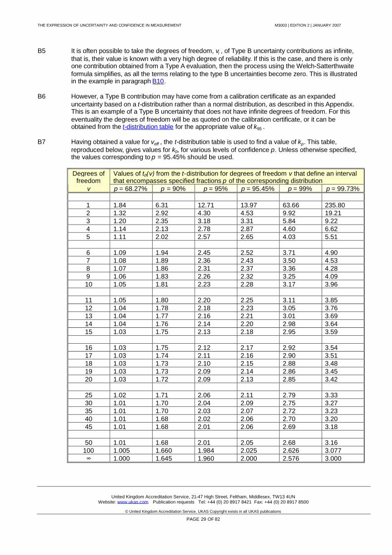
THE EXPRESSION OF UNCERTAINTY AND CONFIDENCE IN MEASUREMENT M3003 | EDITION 2 | JANUARY 2007
United Kingdom Accreditation Service, 21-47 High Street, Feltham, Middlesex, TW13 4UNWebsite: www.ukas.com Publication requests Tel: +44 (0) 20 8917 8421 Fax: +44 (0) 20 8917 8500
© United Kingdom Accreditation Service. UKAS Copyright exists in all UKAS publications
PAGE 29 OF 82
B5 It is often possible to take the degrees of freedom, νi , of Type B uncertainty contributions as infinite,that is, their value is known with a very high degree of reliability. If this is the case, and there is onlyone contribution obtained from a Type A evaluation, then the process using the Welch-Satterthwaiteformula simplifies, as all the terms relating to the type B uncertainties become zero. This is illustratedin the example in paragraph B10.
B6 However, a Type B contribution may have come from a calibration certificate as an expandeduncertainty based on a t-distribution rather than a normal distribution, as described in this Appendix.This is an example of a Type B uncertainty that does not have infinite degrees of freedom. For thiseventuality the degrees of freedom will be as quoted on the calibration certificate, or it can beobtained from the t-distribution table for the appropriate value of k95 .
B7 Having obtained a value for veff , the t-distribution table is used to find a value of kp. This table,reproduced below, gives values for kp, for various levels of confidence p. Unless otherwise specified,the values corresponding to p = 95.45% should be used.
Values of tp(ν) from the t-distribution for degrees of freedom νthat define an intervalthat encompasses specified fractions p of the corresponding distribution
Degrees offreedom
ν p = 68.27% p = 90% p = 95% p = 95.45% p = 99% p = 99.73%
1 1.84 6.31 12.71 13.97 63.66 235.802 1.32 2.92 4.30 4.53 9.92 19.213 1.20 2.35 3.18 3.31 5.84 9.224 1.14 2.13 2.78 2.87 4.60 6.625 1.11 2.02 2.57 2.65 4.03 5.51
6 1.09 1.94 2.45 2.52 3.71 4.907 1.08 1.89 2.36 2.43 3.50 4.538 1.07 1.86 2.31 2.37 3.36 4.289 1.06 1.83 2.26 2.32 3.25 4.0910 1.05 1.81 2.23 2.28 3.17 3.96
11 1.05 1.80 2.20 2.25 3.11 3.8512 1.04 1.78 2.18 2.23 3.05 3.7613 1.04 1.77 2.16 2.21 3.01 3.6914 1.04 1.76 2.14 2.20 2.98 3.6415 1.03 1.75 2.13 2.18 2.95 3.59
16 1.03 1.75 2.12 2.17 2.92 3.5417 1.03 1.74 2.11 2.16 2.90 3.5118 1.03 1.73 2.10 2.15 2.88 3.4819 1.03 1.73 2.09 2.14 2.86 3.4520 1.03 1.72 2.09 2.13 2.85 3.42
25 1.02 1.71 2.06 2.11 2.79 3.3330 1.01 1.70 2.04 2.09 2.75 3.2735 1.01 1.70 2.03 2.07 2.72 3.2340 1.01 1.68 2.02 2.06 2.70 3.2045 1.01 1.68 2.01 2.06 2.69 3.18
50 1.01 1.68 2.01 2.05 2.68 3.16100 1.005 1.660 1.984 2.025 2.626 3.077∞ 1.000 1.645 1.960 2.000 2.576 3.000

THE EXPRESSION OF UNCERTAINTY AND CONFIDENCE IN MEASUREMENT M3003 | EDITION 2 | JANUARY 2007
United Kingdom Accreditation Service, 21-47 High Street, Feltham, Middlesex, TW13 4UNWebsite: www.ukas.com Publication requests Tel: +44 (0) 20 8917 8421 Fax: +44 (0) 20 8917 8500
© United Kingdom Accreditation Service. UKAS Copyright exists in all UKAS publications
PAGE 30 OF 82
B8 Normally veff will not be an integer and it will be necessary to interpolate between the values given inthe table. Linear interpolation will suffice for veff >3; higher-order interpolation should be usedotherwise. Alternatively, the next lower value of veff may be used.
B9 The value of tp(ν) obtained from the table is the coverage factor kp that is required to calculate theexpanded uncertainty, Up, from Up = kp uc(y). Unless otherwise specified, the coverage probability pwill usually be 95%.
B10 Example
B10.1 In a measurement system a Type A evaluation, based on 4 observations, gave a value of ui(y) of 3.5units using Equations (4) and (5). There were 5 other contributions all based on Type B evaluationsfor each of which infinite degrees of freedom had been assumed. The combined standard uncertainty,uc(y), had a value of 5.7 units. Then using the Welch-Satterthwaite formula (paragraph B3, Equation9):
1.2135.37.5
0000014
5.37.5
4
44
4
xeff
B10.2 The value of veff given in the t-distribution table, for a coverage probability p of 95.45%, immediatelylower than 21.1 is 20. This gives a value for kp of 2.13 and this is the coverage factor that should beused to calculate the expanded uncertainty. The expanded uncertainty is 5.7 x 2.13 = 12.14 units.
THE EXPRESSION OF UNCERTAINTY AND CONFIDENCE IN MEASUREMENT M3003 | EDITION 2 | JANUARY 2007
United Kingdom Accreditation Service, 21-47 High Street, Feltham, Middlesex, TW13 4UNWebsite: www.ukas.com Publication requests Tel: +44 (0) 20 8917 8421 Fax: +44 (0) 20 8917 8500
© United Kingdom Accreditation Service. UKAS Copyright exists in all UKAS publications
PAGE 31 OF 82
APPENDIX CDOMINANT NON-GAUSSIAN TYPE B UNCERTAINTY
C1.1 In some measurement processes there can be one component of uncertainty derived from a Type Bevaluation that is dominant in magnitude compared with the other components. When the dominantcomponent is characterised by limits within which there is a high probability of occurrence, acalculated expanded uncertainty, U, using the coverage factor of k = 2, may be greater than thearithmetic sum of the semi-range of all the individual limiting values. As it is reasonable to assumethat the arithmetic sum of these contributions would be for a coverage probability approaching 100%,there is a degree of pessimism in following the normal recommended procedure for combination ofuncertainties.
C1.2 Consequently special consideration needs to be given to the situation in which the calculatedexpanded uncertainty fails to meet the criterion U arithmetic sum of the limit values of allcontributions. For practical purposes, the “limit” value of a normal distribution can be taken as threetimes its standard deviation.
C1.3 In many cases this criterion will be met, but it can be the case that a single rectangular distributionmay dominate over other contributions, A commonly encountered example is the resolution of a
digital indicating instrument. This will have a standard uncertainty of3ia
. If this is large compared to
other contributions it is less likely that the criterion above will be met. When it is not met then thedominant contribution, ad, should be extracted and a new value of the expanded uncertainty shouldbe reported as U = U’ + ad , where U’ is the expanded uncertainty for the remaining components,treated in the normal statistical manner.
C1.4 The use of a two-part expression such as this means that when both components are imported intoa subsequent uncertainty budget it is likely that ad will no longer be a dominant component and anormal distribution can be assumed for the subsequent combined standard uncertainty.
C1.5 Under these circumstances, the statement of coverage probability associated with the expandeduncertainty will have to be modified; an example is given below:
The uncertainty is stated in two parts, the second of which is dominant and is due to the uncertainty due to theresolution of the instrument being calibrated, for which a rectangular probability distribution has been assumed.
C1.6 The same situation may be encountered with other distributions associated with Type B uncertainties.An example is the U-shaped distribution associated with mismatch uncertainty in RF and microwavesystems. Similar reasoning applies here, and the suggested coverage probability statement can bemodified accordingly.
C1.7 There may be, however, situations where a single value of uncertainty is required even if there is aType B uncertainty that causes the distribution to be non-normal. This will involve evaluation of acoverage factor for a stated coverage probability for the convolved distributions.
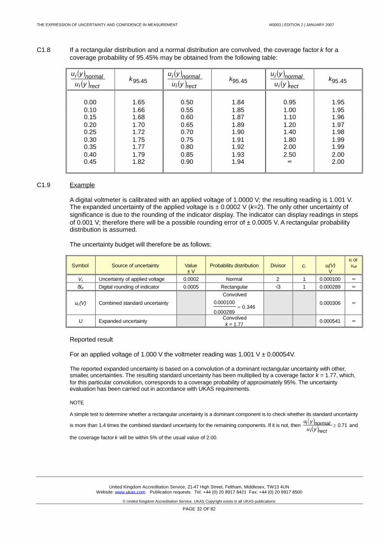
THE EXPRESSION OF UNCERTAINTY AND CONFIDENCE IN MEASUREMENT M3003 | EDITION 2 | JANUARY 2007
United Kingdom Accreditation Service, 21-47 High Street, Feltham, Middlesex, TW13 4UNWebsite: www.ukas.com Publication requests Tel: +44 (0) 20 8917 8421 Fax: +44 (0) 20 8917 8500
© United Kingdom Accreditation Service. UKAS Copyright exists in all UKAS publications
PAGE 32 OF 82
C1.8 If a rectangular distribution and a normal distribution are convolved, the coverage factor k for acoverage probability of 95.45% may be obtained from the following table:
recti
normaliyu
yu45.95k
recti
normaliyu
yu45.95k
recti
normaliyu
yu45.95k
0.00 1.65 0.50 1.84 0.95 1.950.10 1.66 0.55 1.85 1.00 1.950.15 1.68 0.60 1.87 1.10 1.960.20 1.70 0.65 1.89 1.20 1.970.25 1.72 0.70 1.90 1.40 1.980.30 1.75 0.75 1.91 1.80 1.990.35 1.77 0.80 1.92 2.00 1.990.40 1.79 0.85 1.93 2.50 2.000.45 1.82 0.90 1.94 ∞ 2.00
C1.9 Example
A digital voltmeter is calibrated with an applied voltage of 1.0000 V; the resulting reading is 1.001 V.The expanded uncertainty of the applied voltage is ± 0.0002 V (k=2). The only other uncertainty ofsignificance is due to the rounding of the indicator display. The indicator can display readings in stepsof 0.001 V; therefore there will be a possible rounding error of ± 0.0005 V. A rectangular probabilitydistribution is assumed.
The uncertainty budget will therefore be as follows:
Symbol Source of uncertainty Value± V
Probability distribution Divisor ci ui(V)V
νi orνeff
Vs Uncertainty of applied voltage 0.0002 Normal 2 1 0.000100 ∞δId Digital rounding of indicator 0.0005 Rectangular √3 1 0.000289 ∞
uc(V) Combined standard uncertainty
Convolved
346.0000289.0
000100.0
0.000306 ∞
U Expanded uncertaintyConvolvedk = 1.77
0.000541 ∞
Reported result
For an applied voltage of 1.000 V the voltmeter reading was 1.001 V ± 0.00054V.
The reported expanded uncertainty is based on a convolution of a dominant rectangular uncertainty with other,smaller, uncertainties. The resulting standard uncertainty has been multiplied by a coverage factor k = 1.77, which,for this particular convolution, corresponds to a coverage probability of approximately 95%. The uncertaintyevaluation has been carried out in accordance with UKAS requirements.
NOTE
A simple test to determine whether a rectangular uncertainty is a dominant component is to check whether its standard uncertainty
is more than 1.4 times the combined standard uncertainty for the remaining components. If it is not, then 71.0
rectyiunormalyiu
and
the coverage factor k will be within 5% of the usual value of 2.00.
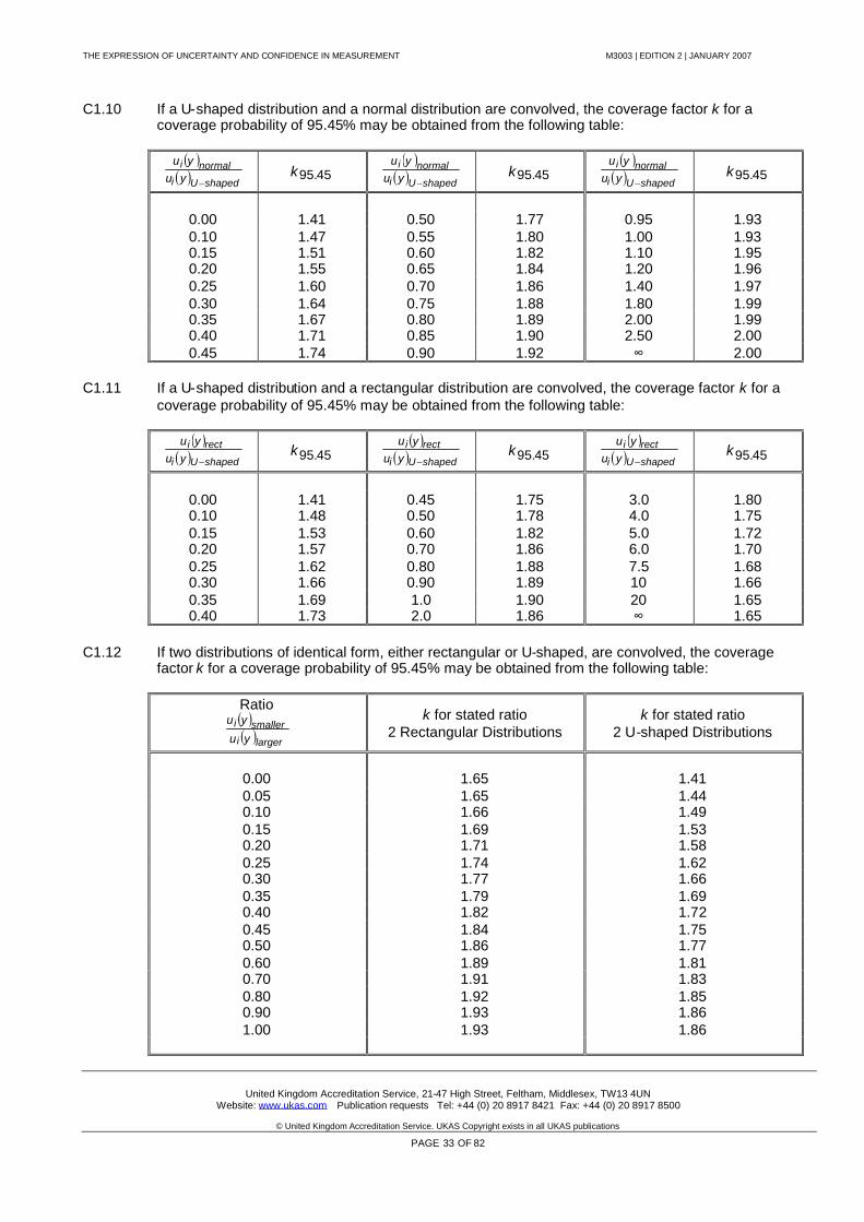
THE EXPRESSION OF UNCERTAINTY AND CONFIDENCE IN MEASUREMENT M3003 | EDITION 2 | JANUARY 2007
United Kingdom Accreditation Service, 21-47 High Street, Feltham, Middlesex, TW13 4UNWebsite: www.ukas.com Publication requests Tel: +44 (0) 20 8917 8421 Fax: +44 (0) 20 8917 8500
© United Kingdom Accreditation Service. UKAS Copyright exists in all UKAS publications
PAGE 33 OF 82
C1.10 If a U-shaped distribution and a normal distribution are convolved, the coverage factor k for acoverage probability of 95.45% may be obtained from the following table:
shapedUi
normaliyu
yu
45.95k
shapedUi
normaliyu
yu
45.95k
shapedUi
normaliyu
yu
45.95k
0.00 1.41 0.50 1.77 0.95 1.930.10 1.47 0.55 1.80 1.00 1.930.15 1.51 0.60 1.82 1.10 1.950.20 1.55 0.65 1.84 1.20 1.960.25 1.60 0.70 1.86 1.40 1.970.30 1.64 0.75 1.88 1.80 1.990.35 1.67 0.80 1.89 2.00 1.990.40 1.71 0.85 1.90 2.50 2.000.45 1.74 0.90 1.92 ∞ 2.00
C1.11 If a U-shaped distribution and a rectangular distribution are convolved, the coverage factor k for acoverage probability of 95.45% may be obtained from the following table:
shapedUi
rectiyu
yu
45.95k
shapedUi
rectiyu
yu
45.95k
shapedUi
rectiyu
yu
45.95k
0.00 1.41 0.45 1.75 3.0 1.800.10 1.48 0.50 1.78 4.0 1.750.15 1.53 0.60 1.82 5.0 1.720.20 1.57 0.70 1.86 6.0 1.700.25 1.62 0.80 1.88 7.5 1.680.30 1.66 0.90 1.89 10 1.660.35 1.69 1.0 1.90 20 1.650.40 1.73 2.0 1.86 ∞ 1.65
C1.12 If two distributions of identical form, either rectangular or U-shaped, are convolved, the coveragefactor k for a coverage probability of 95.45% may be obtained from the following table:
Ratiolargeri
smalleri
yu
yu k for stated ratio2 Rectangular Distributions
k for stated ratio2 U-shaped Distributions
0.00 1.65 1.410.05 1.65 1.440.10 1.66 1.490.15 1.69 1.530.20 1.71 1.580.25 1.74 1.620.30 1.77 1.660.35 1.79 1.690.40 1.82 1.720.45 1.84 1.750.50 1.86 1.770.60 1.89 1.810.70 1.91 1.830.80 1.92 1.850.90 1.93 1.861.00 1.93 1.86
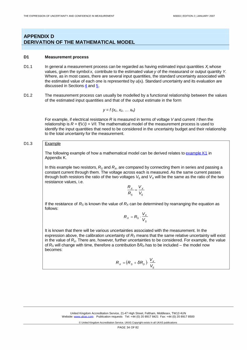
THE EXPRESSION OF UNCERTAINTY AND CONFIDENCE IN MEASUREMENT M3003 | EDITION 2 | JANUARY 2007
United Kingdom Accreditation Service, 21-47 High Street, Feltham, Middlesex, TW13 4UNWebsite: www.ukas.com Publication requests Tel: +44 (0) 20 8917 8421 Fax: +44 (0) 20 8917 8500
© United Kingdom Accreditation Service. UKAS Copyright exists in all UKAS publications
PAGE 34 OF 82
APPENDIX DDERIVATION OF THE MATHEMATICAL MODEL
D1 Measurement process
D1.1 In general a measurement process can be regarded as having estimated input quantities Xi whosevalues, given the symbol x, contribute to the estimated value y of the measurand or output quantity Y.Where, as in most cases, there are several input quantities, the standard uncertainty associated withthe estimated value of each one is represented by u(xi). Standard uncertainty and its evaluation arediscussed in Sections 4 and 5.
D1.2 The measurement process can usually be modelled by a functional relationship between the valuesof the estimated input quantities and that of the output estimate in the form
y = f (x1, x2, … xN)
For example, if electrical resistance R is measured in terms of voltage V and current I then therelationship is R = f(V,I) = V/I. The mathematical model of the measurement process is used toidentify the input quantities that need to be considered in the uncertainty budget and their relationshipto the total uncertainty for the measurement.
D1.3 Example
The following example of how a mathematical model can be derived relates to example K1 inAppendix K.
In this example two resistors, RS and RX, are compared by connecting them in series and passing aconstant current through them. The voltage across each is measured. As the same current passesthrough both resistors the ratio of the two voltages VS and VX will be the same as the ratio of the tworesistance values, i.e.
S
X
S
X
VV
RR
If the resistance of RS is known the value of RX can be determined by rearranging the equation asfollows:
S
XSX V
VRR
It is known that there will be various uncertainties associated with the measurement. In theexpression above, the calibration uncertainty of RS means that the same relative uncertainty will existin the value of RX. There are, however, further uncertainties to be considered. For example, the valueof RS will change with time, therefore a contribution δRD has to be included – the model nowbecomes:
S
XDSX V
VRRR δ
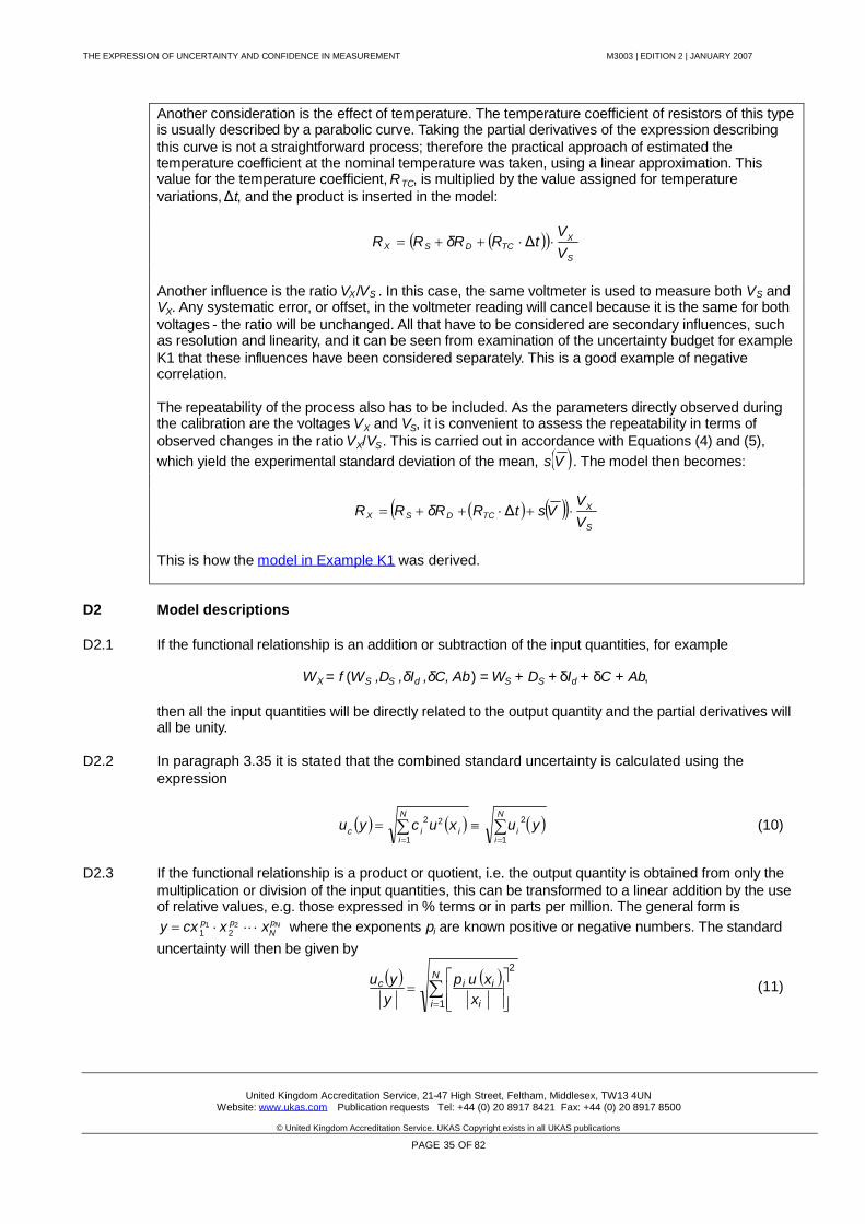
THE EXPRESSION OF UNCERTAINTY AND CONFIDENCE IN MEASUREMENT M3003 | EDITION 2 | JANUARY 2007
United Kingdom Accreditation Service, 21-47 High Street, Feltham, Middlesex, TW13 4UNWebsite: www.ukas.com Publication requests Tel: +44 (0) 20 8917 8421 Fax: +44 (0) 20 8917 8500
© United Kingdom Accreditation Service. UKAS Copyright exists in all UKAS publications
PAGE 35 OF 82
Another consideration is the effect of temperature. The temperature coefficient of resistors of this typeis usually described by a parabolic curve. Taking the partial derivatives of the expression describingthis curve is not a straightforward process; therefore the practical approach of estimated thetemperature coefficient at the nominal temperature was taken, using a linear approximation. Thisvalue for the temperature coefficient, RTC, is multiplied by the value assigned for temperaturevariations, Δt, and the product is inserted in the model:
S
XTCDSX V
VtRRRR Δδ
Another influence is the ratio VX/VS . In this case, the same voltmeter is used to measure both VS andVX. Any systematic error, or offset, in the voltmeter reading will cancel because it is the same for bothvoltages - the ratio will be unchanged. All that have to be considered are secondary influences, suchas resolution and linearity, and it can be seen from examination of the uncertainty budget for exampleK1 that these influences have been considered separately. This is a good example of negativecorrelation.
The repeatability of the process also has to be included. As the parameters directly observed duringthe calibration are the voltages VX and VS, it is convenient to assess the repeatability in terms ofobserved changes in the ratio VX/VS. This is carried out in accordance with Equations (4) and (5),which yield the experimental standard deviation of the mean, Vs . The model then becomes:
S
XTCDSX V
VVstRRRR Δδ
This is how the model in Example K1 was derived.
D2 Model descriptions
D2.1 If the functional relationship is an addition or subtraction of the input quantities, for example
WX = f (WS ,DS ,δId ,δC, Ab) = WS + DS + δId + δC + Ab,
then all the input quantities will be directly related to the output quantity and the partial derivatives willall be unity.
D2.2 In paragraph 3.35 it is stated that the combined standard uncertainty is calculated using theexpression
N
ii
N
iiic yuxucyu
1
2
1
22 (10)
D2.3 If the functional relationship is a product or quotient, i.e. the output quantity is obtained from only themultiplication or division of the input quantities, this can be transformed to a linear addition by the useof relative values, e.g. those expressed in % terms or in parts per million. The general form is
NpN
pp xxcxy 2121 where the exponents pi are known positive or negative numbers. The standard
uncertainty will then be given by
N
i i
iic
xxup
yyu
1
2
(11)
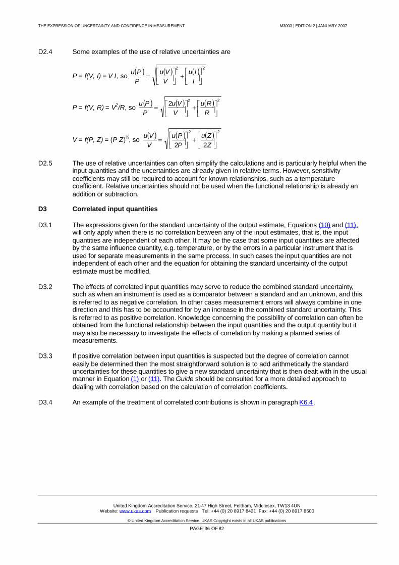
THE EXPRESSION OF UNCERTAINTY AND CONFIDENCE IN MEASUREMENT M3003 | EDITION 2 | JANUARY 2007
United Kingdom Accreditation Service, 21-47 High Street, Feltham, Middlesex, TW13 4UNWebsite: www.ukas.com Publication requests Tel: +44 (0) 20 8917 8421 Fax: +44 (0) 20 8917 8500
© United Kingdom Accreditation Service. UKAS Copyright exists in all UKAS publications
PAGE 36 OF 82
D2.4 Some examples of the use of relative uncertainties are
P = f(V, I) = V·I , so 22
IIu
VVu
PPu
P = f(V, R) = V2/R, so 222
RRu
VVu
PPu
V = f(P, Z) = (P·Z)½, so 22
22
ZZu
PPu
VVu
D2.5 The use of relative uncertainties can often simplify the calculations and is particularly helpful when theinput quantities and the uncertainties are already given in relative terms. However, sensitivitycoefficients may still be required to account for known relationships, such as a temperaturecoefficient. Relative uncertainties should not be used when the functional relationship is already anaddition or subtraction.
D3 Correlated input quantities
D3.1 The expressions given for the standard uncertainty of the output estimate, Equations (10) and (11),will only apply when there is no correlation between any of the input estimates, that is, the inputquantities are independent of each other. It may be the case that some input quantities are affectedby the same influence quantity, e.g. temperature, or by the errors in a particular instrument that isused for separate measurements in the same process. In such cases the input quantities are notindependent of each other and the equation for obtaining the standard uncertainty of the outputestimate must be modified.
D3.2 The effects of correlated input quantities may serve to reduce the combined standard uncertainty,such as when an instrument is used as a comparator between a standard and an unknown, and thisis referred to as negative correlation. In other cases measurement errors will always combine in onedirection and this has to be accounted for by an increase in the combined standard uncertainty. Thisis referred to as positive correlation. Knowledge concerning the possibility of correlation can often beobtained from the functional relationship between the input quantities and the output quantity but itmay also be necessary to investigate the effects of correlation by making a planned series ofmeasurements.
D3.3 If positive correlation between input quantities is suspected but the degree of correlation cannoteasily be determined then the most straightforward solution is to add arithmetically the standarduncertainties for these quantities to give a new standard uncertainty that is then dealt with in the usualmanner in Equation (1) or (11). The Guide should be consulted for a more detailed approach todealing with correlation based on the calculation of correlation coefficients.
D3.4 An example of the treatment of correlated contributions is shown in paragraph K6.4.

THE EXPRESSION OF UNCERTAINTY AND CONFIDENCE IN MEASUREMENT M3003 | EDITION 2 | JANUARY 2007
United Kingdom Accreditation Service, 21-47 High Street, Feltham, Middlesex, TW13 4UNWebsite: www.ukas.com Publication requests Tel: +44 (0) 20 8917 8421 Fax: +44 (0) 20 8917 8500
© United Kingdom Accreditation Service. UKAS Copyright exists in all UKAS publications
PAGE 37 OF 82
APPENDIX ESOME SOURCES OF ERROR AND UNCERTAINTY IN ELECTRICAL CALIBRATIONS
The following is a description of the more common sources of systematic error and uncertainty (aftercorrection) in electrical calibration work, with brief comments about their nature. Further, more detailed,advice is given in specialised technical publications and manufacturers’ application notes, as well as othersources.
E1 Imported uncertainty
E1.1 The uncertainties assigned to the values on a calibration certificate for the calibration of an instrument,whether measuring equipment or a reference standard, are all contributors to the uncertainty budget.
E2 Secular stability
E2.1 The performance of all instruments, and the values of reference standards, must be expected to changeto some extent with the passage of time. Passive devices such as standard resistors or high-grade RFand microwave attenuators may be expected to drift slowly with time. An estimate of such a drift has tobe assessed on the basis of values obtained from previous calibrations. It cannot be assumed that a driftwill be linear. Data can be assimilated readily if displayed in a graphical form. A curve fitting procedurethat gives a progressively greater weight to each of the more recent calibrations can be used to allow themost probable value at the time of use to be assessed. The degree of complexity in curve fitting is amatter of judgement; in some cases drawing a smooth curve through the chosen data points by handcan be quite satisfactory. Whenever a new calibration is obtained the drift characteristic will need re-assessment. The corrections that are applied for drift are subject to uncertainty based on the scatter ofdata points about the drift characteristic. The magnitude of the drift and the random instability of aninstrument, and the accuracy required will determine the calibration interval.
E2.2 With complex electronic equipment it is not always possible to follow this procedure as changes inperformance can be expected to be more random in nature over relatively long periods. Checks againstpassive standards can establish whether compliance to specification is being maintained or whether acalibration with subsequent equipment adjustment is needed. The manufacturer’s specification can be agood starting point for assigning the uncertainty due to instrument drift, but should be confirmed byanalysis of quality control and calibration data.
E3 Environmental conditions
E3.1 The laboratory measurement environment can be one of the most important considerations whenperforming electrical calibrations. Ambient temperature is often the most important influence andinformation on the temperature coefficient of, for example, resistance standards has to be sought ordetermined. Variations in relative humidity can also affect the values of unsealed components. Theinfluence of barometric pressure on certain electrical measurement standards can also be significant. AtRF and microwave frequencies, ambient temperature can affect the performance of, for example,attenuators, impedance standards that depend on mechanical dimensions for their values and otherprecision components. Devices that incorporate thermal sensing, such as power sensors, can be affectedby rapid temperature changes that can be introduced by handling or exposure to sunlight or other sourcesof heat.
THE EXPRESSION OF UNCERTAINTY AND CONFIDENCE IN MEASUREMENT M3003 | EDITION 2 | JANUARY 2007
United Kingdom Accreditation Service, 21-47 High Street, Feltham, Middlesex, TW13 4UNWebsite: www.ukas.com Publication requests Tel: +44 (0) 20 8917 8421 Fax: +44 (0) 20 8917 8500
© United Kingdom Accreditation Service. UKAS Copyright exists in all UKAS publications
PAGE 38 OF 82
E3.2 It is also necessary to be aware of the possible effects of electrical operating conditions, such as powerdissipation, harmonic distortion, or level of applied voltage being different when a device is in use fromwhen it was calibrated. Resistance standards, resistive voltage dividers and attenuators at any frequencyare examples of devices being affected by self-heating and/or applied voltage. It should also be ensuredthat all equipment is operating within the manufacturer's stated range of supply voltages.
E3.3 The effects of harmonics and noise on ac calibration signals may have an influence on the apparent valueof these signals. Similarly, the effects of any common-mode signals present in a measurement system mayhave to be accounted for.
E4 Interpolation of calibration data
E4.1 When an instrument with a broad range of measurement capabilities is calibrated there are practical andeconomic factors that limit the number of calibration points. Consequently the value of the quantity to bemeasured and/or its frequency may be different from any of the calibration points. When the value of thequantity lies between two calibration values, consideration needs to be given to systematic errors that arisefrom, for example, scale non-linearity.
E4.2 If the measurement frequency falls between two calibration frequencies, it will also be necessary to assessthe additional uncertainty due to interpolation that this can introduce. One can only proceed withconfidence if:
(a) a theory of instrument operation is known from which one can predict a frequency characteristic, or there isadditional frequency calibration data from other models of the same instrument,
and wherever reasonable,
(b) the performance of the actual instrument being used has been explored with a swept frequencymeasurement system to verify the absence of resonance effects or aberrations due to manufacturing orother performance limitations.
E5 Resolution
E5.1 The limit to the ability of an instrument to indicate small changes in the quantity being measured, referredto as resolution or “digital rounding error”, is treated as a systematic component of uncertainty.
E5.2 Many instruments with a digital display use an analogue-to digital converter (ADC) to convert theanalogue signal under investigation into a form that can be displayed in terms of numeric digits. The lastdisplayed digit will be a rounded representation of the underlying analogue signal. The error introducedby this process will be from - 0.5 digit (else the last digit would be one lower) to + 0.5 digit (else the lastdigit would be one higher). A quantisation error of ± 0.5 digit is therefore present. As there is no way ofknowing where within this range the underlying value is, the resulting error is assumed to be zero withlimits of ± 0.5 digit.
E5.3 This “digital rounding error” of ± 0.5 digit may not apply in all instances and an understanding ofinstrument operation is needed if the assigned uncertainty is to be realistic. For example, a direct-gatingfrequency counter has a digital rounding error of ± 1 digit, due to the random relationship between thesignal being measured and the internal clock. Some instruments may also display hysteresis that,although not necessarily a property of the display itself, may result in further uncertainties amounting toseveral digits.
E5.4 In an analogue instrument the effect of resolution is determined by the practical ability to read the positionof a pointer on a scale. In either case, the last digit actually recorded will always be subject to anuncertainty of at least ± 0.5 digit. The presence of electrical noise causing fluctuations in instrumentreadings will commonly determine the usable resolution, however it is possible to make a good estimate ofthe mean position of a fluctuating pointer by eye.
THE EXPRESSION OF UNCERTAINTY AND CONFIDENCE IN MEASUREMENT M3003 | EDITION 2 | JANUARY 2007
United Kingdom Accreditation Service, 21-47 High Street, Feltham, Middlesex, TW13 4UNWebsite: www.ukas.com Publication requests Tel: +44 (0) 20 8917 8421 Fax: +44 (0) 20 8917 8500
© United Kingdom Accreditation Service. UKAS Copyright exists in all UKAS publications
PAGE 39 OF 82
E6 Apparatus layout
E6.1 The physical layout of one item of equipment with respect to another and the relationship of these items tothe earth plane can be important in some measurements. Thus a different arrangement betweencalibration and subsequent use of an instrument may be the source of systematic errors. The main effectsare leakage currents to earth, interference loop currents, and electromagnetic leakage fields. In inductancemeasurements it is necessary to define connecting lead configuration and be conscious of the possibleeffects of an earth plane or adjacent ferromagnetic material. The effect of mutual heating betweenapparatus may also need to be considered.
E7 Thermoelectric voltages
E7.1 If an electrical conductor passes through a temperature gradient then a potential difference will begenerated across that gradient. This is known as the Seebeck effect and these unwanted, parasiticvoltages can cause errors in some measurement systems – in particular, where small dc voltages arebeing measured.
E7.2 They can be minimised by design of connections that are thermally symmetrical, so that the Seebeckvoltage in one lead is cancelled by an identical and opposite voltage in the other. In some situations, e.g.ac/dc transfer measurements, the polarity of the dc supply is reversed and an arithmetic mean is taken oftwo sets of dc measurements.
E7.3 Generally an allowance has to be made as a Type B component of uncertainty for the presence of thermalemfs.
E8 Loading and cable impedance
E8.1 The finite input impedance of voltmeters, oscilloscopes and other voltage sensing instruments may so loadthe circuit to which they are connected as to cause significant systematic errors. Corrections may bepossible if impedances are known. In particular, it should be noted that some multi-function calibrators canexhibit a slightly inductive output impedance. This means that when a capacitive load is applied, theresulting resonance may cause the output voltage to increase with respect to its open-circuit value.
E8.2 The impedance and finite electrical length of connecting leads or cables may also result in systematicerrors in voltage measurements at any frequency. The use of four-terminal connections minimises sucherrors in some dc and ac measurements.
E8.3 For capacitance measurements, the inductive properties of the connecting leads may be important,particularly at higher values of capacitance and/or frequency. Similarly, for inductance measurements thecapacitance between connecting leads may be important.
E9 RF mismatch errors and uncertainty
E9.1 At RF and microwave frequencies the mismatch of components to the characteristic impedance of themeasurement system transmission line can be one of the most important sources of error and of thesystematic component of uncertainty in power and attenuation measurements. This is because the phasesof voltage reflection coefficients are not usually known and hence corrections cannot be applied.
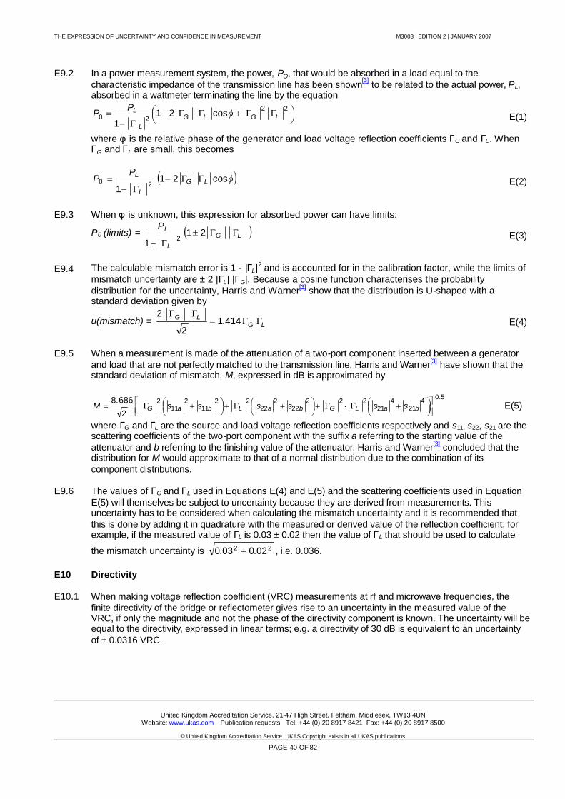
THE EXPRESSION OF UNCERTAINTY AND CONFIDENCE IN MEASUREMENT M3003 | EDITION 2 | JANUARY 2007
United Kingdom Accreditation Service, 21-47 High Street, Feltham, Middlesex, TW13 4UNWebsite: www.ukas.com Publication requests Tel: +44 (0) 20 8917 8421 Fax: +44 (0) 20 8917 8500
© United Kingdom Accreditation Service. UKAS Copyright exists in all UKAS publications
PAGE 40 OF 82
E9.2 In a power measurement system, the power, PO, that would be absorbed in a load equal to thecharacteristic impedance of the transmission line has been shown[3] to be related to the actual power, PL,absorbed in a wattmeter terminating the line by the equation
22
20 cos211
LGLGL
LPP E(1)
where φis the relative phase of the generator and load voltage reflection coefficients ΓG and ΓL. WhenΓG and ΓL are small, this becomes
cos211 20 LG
L
LPP
E(2)
E9.3 When φis unknown, this expression for absorbed power can have limits:
P0 (limits) = LG
L
LP
21
1 2 E(3)
E9.4 The calculable mismatch error is 1 - |ΓL|2 and is accounted for in the calibration factor, while the limits ofmismatch uncertainty are ± 2 |ΓL| |ΓG|. Because a cosine function characterises the probabilitydistribution for the uncertainty, Harris and Warner[3] show that the distribution is U-shaped with astandard deviation given by
u(mismatch) = LGLG
414.12
2E(4)
E9.5 When a measurement is made of the attenuation of a two-port component inserted between a generatorand load that are not perfectly matched to the transmission line, Harris and Warner[3] have shown that thestandard deviation of mismatch, M, expressed in dB is approximated by
5.0421
421
22222
222
2211
211
2
2
686.8
baLGbaLbaG ssssssM E(5)
where ΓG and ΓL are the source and load voltage reflection coefficients respectively and s11, s22, s21 are thescattering coefficients of the two-port component with the suffix a referring to the starting value of theattenuator and b referring to the finishing value of the attenuator. Harris and Warner[3] concluded that thedistribution for M would approximate to that of a normal distribution due to the combination of itscomponent distributions.
E9.6 The values of ΓG and ΓL used in Equations E(4) and E(5) and the scattering coefficients used in EquationE(5) will themselves be subject to uncertainty because they are derived from measurements. Thisuncertainty has to be considered when calculating the mismatch uncertainty and it is recommended thatthis is done by adding it in quadrature with the measured or derived value of the reflection coefficient; forexample, if the measured value of ΓL is 0.03 ± 0.02 then the value of ΓL that should be used to calculate
the mismatch uncertainty is 22 02.003.0 , i.e. 0.036.
E10 Directivity
E10.1 When making voltage reflection coefficient (VRC) measurements at rf and microwave frequencies, thefinite directivity of the bridge or reflectometer gives rise to an uncertainty in the measured value of theVRC, if only the magnitude and not the phase of the directivity component is known. The uncertainty will beequal to the directivity, expressed in linear terms; e.g. a directivity of 30 dB is equivalent to an uncertaintyof ± 0.0316 VRC.
THE EXPRESSION OF UNCERTAINTY AND CONFIDENCE IN MEASUREMENT M3003 | EDITION 2 | JANUARY 2007
United Kingdom Accreditation Service, 21-47 High Street, Feltham, Middlesex, TW13 4UNWebsite: www.ukas.com Publication requests Tel: +44 (0) 20 8917 8421 Fax: +44 (0) 20 8917 8500
© United Kingdom Accreditation Service. UKAS Copyright exists in all UKAS publications
PAGE 41 OF 82
E10.1 As with E9.6 above it is recommended that the uncertainty in the measurement of directivity is taken intoaccount by adding the measured value in quadrature with the uncertainty, in linear quantities; for example,if the measured directivity of a bridge is 36 dB (0.016) and has an uncertainty of +8 dB -4 dB (± 0.01) then
the directivity to be used is 22 01.0016.0 = 0.019 (34.4 dB).
E11 Test port match
E11.1 The test port match of a bridge or reflectometer used for reflection coefficient measurements will give riseto an error in the measured VRC due to re-reflection. The uncertainty, u(TP), is calculated from u(TP) =TP.ΓX
2 where TP is the test port match, expressed as a VRC, and ΓX is the measured reflection coefficient.When a directional coupler is used to monitor incident power in the calibration of a power meter it is theeffective source match of the coupler that defines the value of ΓG referred to in E9. As with E9.6 and E10,the measured value of test port match will have an uncertainty that should be taken into account by usingquadrature summation.
E12 RF connector repeatability
The lack of repeatability of coaxial pair insertion loss and, to a lesser extent, voltage reflection coefficient isa problem when calibrating devices in a coaxial line measurement system and subsequently using them insome other system. Although connecting and disconnecting the device can evaluate the repeatability ofparticular connector pairs in use, these connector pairs are only samples from a whole population. Toobtain representative data for guidance for various types of connectors in use is beyond the resources ofmost measurement laboratories. Reference [5] provides advice on the specifications and use of coaxialconnectors including guidance on the repeatability of the insertion loss of connector pairs.
THE EXPRESSION OF UNCERTAINTY AND CONFIDENCE IN MEASUREMENT M3003 | EDITION 2 | JANUARY 2007
United Kingdom Accreditation Service, 21-47 High Street, Feltham, Middlesex, TW13 4UNWebsite: www.ukas.com Publication requests Tel: +44 (0) 20 8917 8421 Fax: +44 (0) 20 8917 8500
© United Kingdom Accreditation Service. UKAS Copyright exists in all UKAS publications
PAGE 42 OF 82
APPENDIX FSOME SOURCES OF ERROR AND UNCERTAINTY IN MASS CALIBRATIONS
This Appendix describes the more common sources of errors and uncertainties in mass calibration withbrief comments about their nature. They may not all be significant at all levels of measurement, but theireffect should at least be considered when estimating the overall uncertainty of a measurement. Furtherinformation about mass calibration can be found in reference [6].
F1 Reference weight calibration
F1.1 The uncertainties assigned to the values on a calibration certificate for the calibration of the referenceweights are all contributors to the uncertainty budget.
F2 Secular stability of reference weights
F2.1 It is necessary to take into account the likely change in mass of the reference weights since their lastcalibration. This change can be estimated from the results of successive calibrations of the referenceweights. If such a history is not available, then it is usual to assume that they may change in mass by anamount equal to their uncertainty of calibration between calibrations. The stability of weights can beaffected by the material and quality of manufacture (e.g., ill-fitting screw knobs), surface finish, unstableadjustment material, physical wear and damage and atmospheric contamination. The figure adopted forstability will need to be reconsidered if the usage or environment of the weights changes. The calibrationinterval for reference weights will depend on the stability of the weights.
F3 Weighing machine/weighing process
F3.1 The performance of the weighing machine used for the calibration should be assessed to estimate thecontribution it makes to the overall uncertainty of the weighing process. The performance assessmentshould cover those attributes of the weighing machine that are significant to the weighing process. Forexample, the length of arm error (assuming it is constant) of an equal arm balance need not be assessed ifthe weighing process only uses substitution techniques (Borda's method). The assessment may includesome or all of the following:
(a) repeatability of measurement;
(b) linearity within the range used;
(c) digit size/weight value per division, i.e. readability;
(d) eccentricity (off centre load), especially if groups of weights are placed on the weighing pansimultaneously;
(e) magnetic effects (e.g. magnetic weights, or the effect of force balance motors on cast iron weights);
(f) temperature effects, e.g. differences between the temperature of the weights and the weighing machine;
(f) length of arm error.
THE EXPRESSION OF UNCERTAINTY AND CONFIDENCE IN MEASUREMENT M3003 | EDITION 2 | JANUARY 2007
United Kingdom Accreditation Service, 21-47 High Street, Feltham, Middlesex, TW13 4UNWebsite: www.ukas.com Publication requests Tel: +44 (0) 20 8917 8421 Fax: +44 (0) 20 8917 8500
© United Kingdom Accreditation Service. UKAS Copyright exists in all UKAS publications
PAGE 43 OF 82
F4 Air buoyancy effects
F4.1 The accuracy with which air buoyancy corrections can be made depends on how well the density of theweights is known, and how well the air density can be determined. Some laboratories can determine thedensity of weights, but for most mass work assumed figures are used. The air density is usually calculatedfrom an equation (see reference [6]) after measuring the air temperature, pressure and humidity. For thehighest levels of accuracy, it may also be necessary to measure the carbon dioxide content of the air. Thefigures that follow are based upon an air density range of 1.079 kg m -3 to 1.291 kg m-3 which can beproduced by ranges of relative humidity from 30% to 70%, air temperature from 10C to 30C andbarometric pressure from 950 millibar to 1050 millibar.
F4.2 For mass comparisons a figure of ± 1 part in 106 of the applied mass is typical for common weightmaterials such as stainless steel, plated brass, German silver and gunmetal. For cast iron the figure maybe up to ± 3 parts in 106 and for aluminium up to ± 30 parts in 106. The uncertainty can be reduced if themass comparisons are made within suitably restricted ranges of air temperature, pressure and humidity. Ifcorrections are made for the buoyancy effects the uncertainty can be virtually eliminated, leaving just theuncertainty of the correction.
F4.3 Certain weighing machines display mass units directly from the force they experience when weights areapplied. It is common practice to reduce the effects of buoyancy on such devices by the use of an auxiliaryweight, known as a spanning weight, which is used to normalise the readings to the prevailing conditions,as well as compensating for changes in the machine itself. This spanning weight can be external or internalto the machine. If such machines are not spanned at the time of use the calibration may be subject to anincreased uncertainty due to the buoyancy effects on the loading weights. For weighing machines thatmake use of stainless steel, plated brass, German silver or gunmetal weights this effect may be up to ±16parts in 106. For cast iron weights the figure may be up to ±18 parts in 106 and for aluminium weights up to± 45 parts in 106.
F4.4 For the ambient conditions stated above the uncertainty limits due to buoyancy effects may be ± 110 partsin 106 and ± 140 parts in 106 respectively for comparing water and organic solvents with stainless steelmass standards, and ± 125 parts in 106 and ± 155 parts in 106 respectively for direct weighing.
F4.5 Apart from air buoyancy effects, the environment in which the calibration takes place can introduceuncertainties. Temperature gradients can give rise to convection currents in the balance case, which willaffect the reading, as will draughts from air conditioning units. Rapid changes of temperature in thelaboratory can affect the weighing process. Changes in the level of humidity in the laboratory can makeshort-term changes to the mass of weights, while low levels of humidity can introduce static electricityeffects on some comparators. Dust contamination also introduces errors in calibrations. The movement ofweights during the calibration causes disturbances to the local environment.
THE EXPRESSION OF UNCERTAINTY AND CONFIDENCE IN MEASUREMENT M3003 | EDITION 2 | JANUARY 2007
United Kingdom Accreditation Service, 21-47 High Street, Feltham, Middlesex, TW13 4UNWebsite: www.ukas.com Publication requests Tel: +44 (0) 20 8917 8421 Fax: +44 (0) 20 8917 8500
© United Kingdom Accreditation Service. UKAS Copyright exists in all UKAS publications
PAGE 44 OF 82
APPENDIX GSOME SOURCES OF ERROR AND UNCERTAINTY IN TEMPERATURE CALIBRATIONS
The more common sources of systematic error and uncertainty in the measurement of temperature aredescribed in this section. Each source may have several uncertainty components.
G1 Reference thermometer calibration
G1.1 The uncertainties assigned to the values on a calibration certificate for the calibration of the referencethermometer are all contributors to the uncertainty budget.
G2 Measuring instruments
G2.1 The uncertainty assigned to the calibration of any electrical or other instruments used in themeasurements, e.g. standard resistors, measuring bridges and digital multimeters.
G3 Further influences
G3.1 Additional uncertainties in the measurement of the temperature using the reference thermometers:
(a) Drift since the last calibration of the reference thermometers and any associated measuring instruments;
(b) Resolution of reading; this may be very significant in the case of a liquid-in-glass thermometer or digitalthermometers;
(c) Instability and temperature gradients in the thermal environment, e.g., the calibration bath or furnace,including any contribution due to difference in immersion of the reference standard from that stated on itscertificate of calibration;
(d) When platinum resistance thermometers are used as reference standards any contribution to theuncertainty due to self-heating effects should be considered. This will mainly apply if the measuring currentis different from that used in the original calibration and/or the conditions of measurement e.g., `in air' or instirred liquid.
G4 Contributions associated with the thermometer to be calibrated
G4.1 These may include factors associated with electrical indicators as well as some of the further influencesalready mentioned. When partial immersion liquid-in-glass thermometers are to be calibrated an additionaluncertainty contribution to account for effects arising from differences in depth of immersion should beincluded even when the emergent column temperature is measured.
G4.2 When thermocouples are being calibrated any uncertainty introduced by compensating leads andreference junctions should be taken into account. Similarly any thermal emfs introduced by switches orscanner units should be investigated. Unknown errors arising from inhomogeneity of the thermocouplebeing calibrated can give rise to significant uncertainties. Ideally this should be evaluated at the time ofcalibration, possibly by varying the immersion depth of the thermocouple in an isothermal enclosure. Formany calibrations, however, this will not be practical. In such cases, a figure of 20% of the maximumpermissible error for the particular thermocouple type is considered reasonable.
G5 Mathematical interpretation
G5.1 Uncertainty arising from mathematical interpretation, e.g. in applying scale corrections or deviations from areference table, or in curve-fitting to allow for scale non-linearity, should be assessed.

THE EXPRESSION OF UNCERTAINTY AND CONFIDENCE IN MEASUREMENT M3003 | EDITION 2 | JANUARY 2007
United Kingdom Accreditation Service, 21-47 High Street, Feltham, Middlesex, TW13 4UNWebsite: www.ukas.com Publication requests Tel: +44 (0) 20 8917 8421 Fax: +44 (0) 20 8917 8500
© United Kingdom Accreditation Service. UKAS Copyright exists in all UKAS publications
PAGE 45 OF 82
APPENDIX HSOME SOURCES OF ERROR AND UNCERTAINTY IN DIMENSIONAL CALIBRATIONS
The more common sources of systematic error and uncertainty in dimensional measurements aredescribed in this section.
H1 Reference standards and Instrumentation
H1.1 The uncertainties assigned to the reference standards and those for the measuring instruments used tomake the measurements.
H2 Secular stability of reference standards and instrumentation
H2.1 The changes that occur over time must be taken into account, usually by reference to the calibrationhistory of the equipment. This is particularly important when the equipment may be exposed to physicalwear as part of normal operation.
H3 Temperature effects
H3.1 The uncertainties associated with differences in temperature between the gauge being calibrated and thereference standards and measuring instruments used should be accounted for. These will be mostsignificant over the longer lengths and in cases involving dissimilar materials. Whilst it may be possible tomake corrections for temperature effects there will be residual uncertainties resulting from uncertainty inthe values used for the coefficients of expansion and the calibration of the measuring thermometer.
H4 Elastic compression
H4.1 These are uncertainties associated with differences in elastic compression between the materials fromwhich the gauge being calibrated and the reference standards were manufactured. They are likely to bemost significant in the more precise calibrations and in cases involving dissimilar materials. They will relateto the measuring force used and the nature of stylus contact with the gauge and reference standard. Whilstmathematical corrections can be made there will be residual uncertainties resulting from the uncertainty ofthe measuring force and in the properties of the materials involved.
H5 Cosine errors
H5.1 Any misalignment of the gauge being calibrated or reference standards used, with respect to the axis ofmeasurement, will introduce errors into the measurements. Such errors are often referred to as cosineerrors and can be minimised by adjusting the attitude of the gauge with respect to the axis of measurementto find the relevant turning points that give the appropriate maximum or minimum result. Small residualerrors can still result where, for instance, incorrect assumptions are made concerning any features used foralignment of the datums.
H6 Geometric errors
H6.1 Errors in the geometry of the gauge being calibrated, any reference standards used or critical features ofthe measuring instruments used to make the measurements can introduce additional uncertainties.Typically these will include small errors in the flatness or sphericity of stylus tips, the straightness, flatness,parallelism or squareness of surfaces used as datum features, and the roundness or taper in cylindricalgauges and reference standards. Such errors are often most significant in cases where perfect geometryhas been wrongly assumed and where the measurement methods chosen do not capture, suppress orotherwise accommodate the geometric errors that prevail in a particular case.
THE EXPRESSION OF UNCERTAINTY AND CONFIDENCE IN MEASUREMENT M3003 | EDITION 2 | JANUARY 2007
United Kingdom Accreditation Service, 21-47 High Street, Feltham, Middlesex, TW13 4UNWebsite: www.ukas.com Publication requests Tel: +44 (0) 20 8917 8421 Fax: +44 (0) 20 8917 8500
© United Kingdom Accreditation Service. UKAS Copyright exists in all UKAS publications
PAGE 46 OF 82
APPENDIX JSOME SOURCES OF ERROR AND UNCERTAINTY IN PRESSURE CALIBRATIONSUSING DEAD WEIGHT TESTERS
The more common sources of systematic error and uncertainty in the generation of known pressures,using dead weight testers (DWT), are described in this section.
J1 Reference DWT
J1.1 The uncertainties assigned to the values on a calibration certificate for the reference dead weight testerare all contributors to the uncertainty budget. These include the following:
(a) Area uncertainty including any uncertainty in the distortion. This uncertainty will often vary with pressure;
(b) Piston and weight carrier mass.
J2 Secular stability of the reference dead weight tester
J2.1 It is necessary to account for likely changes in the area and mass of the reference DWT since the lastcalibration. This change can be estimated from successive calibrations of the reference DWT. Thesecular stability uncertainty for the area will depend on the calibration interval and can be larger than thecalibration uncertainty. The variation between calibrations in the area of a DWT will depend on its usage,design, and material composition and is therefore a best estimate from actual data. Where this is notavailable it is recommended that a pessimistic estimate is made and a short calibration interval set.
J2.2 The drift of the piston mass will be larger in oil DWTs as this will reflect the difficulties in repeat weightingof pistons that have been immersed in oil. These difficulties arise from incomplete cleaning processesand possible instability due to the evaporation of solvents.
J3 Reference DWT mass set uncertainty
J3.1 The uncertainties assigned to the values on a calibration certificate for the weights in the reference deadweight tester mass set are all contributors to the uncertainty budget. The uncertainty of the mass stackused to generate pressure should be evaluated over the range of the DWT. The relative uncertainty isoften higher at lower pressures.
J4 Secular stability of the reference DWT mass set
J4.1 It is necessary to account for likely changes the mass set of the reference DWT since the lastcalibration. Paragraph F2.1 addresses the subject of secular stability of reference weights.
J5 Uncertainty of local gravity determination
J5.1 The pressure generated by a DWT is directly affected by the local acceleration due to gravity, g. Withcare, this can be measured with an uncertainty of less than 1 ppm. It is possible for an estimate of the gvalue to be obtained from a reputable geological survey organisation based on a grid reference; thiswould attract an uncertainty of around 3 ppm. It can also be calculated from knowledge of latitude andaltitude, however the uncertainty will be much larger - around 50 ppm in the UK. Some knowledge of theBouguer anomalies is required to achieve these levels of uncertainty from such calculations.
THE EXPRESSION OF UNCERTAINTY AND CONFIDENCE IN MEASUREMENT M3003 | EDITION 2 | JANUARY 2007
United Kingdom Accreditation Service, 21-47 High Street, Feltham, Middlesex, TW13 4UNWebsite: www.ukas.com Publication requests Tel: +44 (0) 20 8917 8421 Fax: +44 (0) 20 8917 8500
© United Kingdom Accreditation Service. UKAS Copyright exists in all UKAS publications
PAGE 47 OF 82
J6 Air buoyancy effect
J6.1 Air buoyancy affects the mass set of a DWT in the same way as described in paragraph F4.
J7 Temperature effect on DWT area
J7.1 The area on a DWT changes with temperature; its temperature coefficient of expansion being related tothe particular materials that the piston and cylinder are made from. Consideration has to be given to anyvariation in temperature from the reference temperature when the DWT was calibrated, variation intemperature during a calibration and uncertainty in the determination of the piston temperature.
J8 Uncertainty due to head correction
J8.1 Any difference between the height of the reference DWT datum level and that of the item beingcalibrated will affect the pressure generated at that item. For pneumatic calibrations this effect isproportional to pressure and normally equates to about 116 ppm/m. For hydraulic calibrations the effectis a fixed pressure effect that will depend on the density of the fluid used, local acceleration due togravity and the height difference. (Fluid head pressure = ρ.g.h) For most DWT oils the effect is between8 and 9 Pa/mm.
J8.2 The float height position of the piston will also contribute to the head correction uncertainty. This effectwill be related to the fall rate of the piston and the particular measurement procedure in use.
J9 Effects of fluid properties
J9.1 For hydraulic calibrations the effect of the fluid properties on fluid head corrections, buoyancy volumecorrections and surface tension corrections will also need to be considered. These figures are usuallyreported on calibration certificates for DWTs. However, care must be taken to convert any quotedcorrection to the actual oil used if different from that used during the calibration of the reference DWT. Inmost circumstances the uncertainty of these influence quantities can be treated as negligible.
J10 Non-verticality of the DWT piston
An uncertainty arises due to the fact that the piston may not be perfectly vertical. If it were, then all of theforce would act on the area. Any departure from vertical will reduce the force and therefore the generatedpressure. The effect in terms of generated pressure is proportional to the cosine of the angle from truevertical.
J11 Uncertainties arising from the calibration process
J11.1 Any uncertainty arising from the calibration process will need to be evaluated. These could include theresolution and repeatability of the unit being calibrated and the effects of the environment on it.Uncertainties due to calculation or data fitting of the calibration results may also have to be considered.
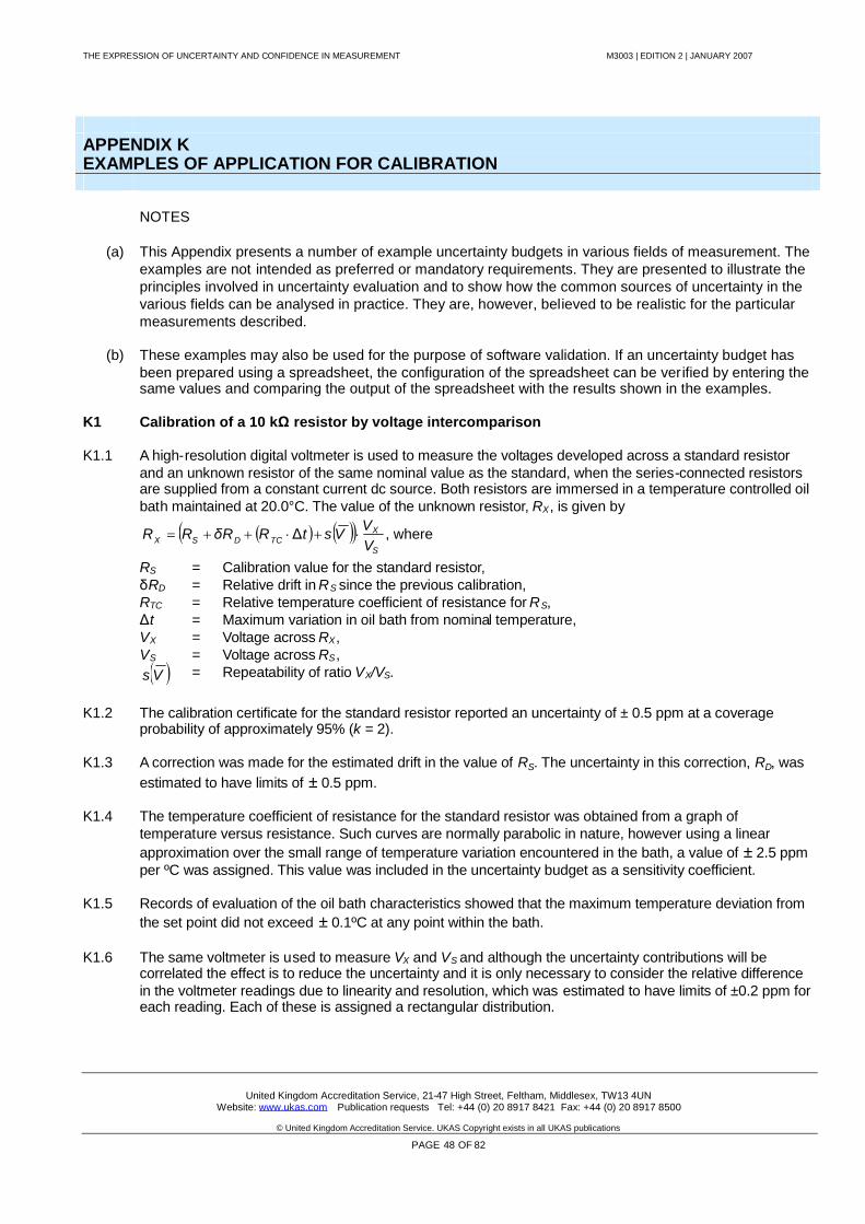
THE EXPRESSION OF UNCERTAINTY AND CONFIDENCE IN MEASUREMENT M3003 | EDITION 2 | JANUARY 2007
United Kingdom Accreditation Service, 21-47 High Street, Feltham, Middlesex, TW13 4UNWebsite: www.ukas.com Publication requests Tel: +44 (0) 20 8917 8421 Fax: +44 (0) 20 8917 8500
© United Kingdom Accreditation Service. UKAS Copyright exists in all UKAS publications
PAGE 48 OF 82
APPENDIX KEXAMPLES OF APPLICATION FOR CALIBRATION
NOTES
(a) This Appendix presents a number of example uncertainty budgets in various fields of measurement. Theexamples are not intended as preferred or mandatory requirements. They are presented to illustrate theprinciples involved in uncertainty evaluation and to show how the common sources of uncertainty in thevarious fields can be analysed in practice. They are, however, believed to be realistic for the particularmeasurements described.
(b) These examples may also be used for the purpose of software validation. If an uncertainty budget hasbeen prepared using a spreadsheet, the configuration of the spreadsheet can be verified by entering thesame values and comparing the output of the spreadsheet with the results shown in the examples.
K1 Calibration of a 10 kΩresistor by voltage intercomparison
K1.1 A high-resolution digital voltmeter is used to measure the voltages developed across a standard resistorand an unknown resistor of the same nominal value as the standard, when the series-connected resistorsare supplied from a constant current dc source. Both resistors are immersed in a temperature controlled oilbath maintained at 20.0°C. The value of the unknown resistor, RX, is given by
S
XTCDSX V
VVstRRRR Δδ , where
RS
δRD
RTC
ΔtVX
VS
Vs
=======
Calibration value for the standard resistor,Relative drift in RS since the previous calibration,Relative temperature coefficient of resistance for RS,Maximum variation in oil bath from nominal temperature,Voltage across RX,Voltage across RS,Repeatability of ratio VX/VS.
K1.2 The calibration certificate for the standard resistor reported an uncertainty of ± 0.5 ppm at a coverageprobability of approximately 95% (k = 2).
K1.3 A correction was made for the estimated drift in the value of RS. The uncertainty in this correction, RD, wasestimated to have limits of ± 0.5 ppm.
K1.4 The temperature coefficient of resistance for the standard resistor was obtained from a graph oftemperature versus resistance. Such curves are normally parabolic in nature, however using a linearapproximation over the small range of temperature variation encountered in the bath, a value of ± 2.5 ppmper ºC was assigned. This value was included in the uncertainty budget as a sensitivity coefficient.
K1.5 Records of evaluation of the oil bath characteristics showed that the maximum temperature deviation fromthe set point did not exceed ± 0.1ºC at any point within the bath.
K1.6 The same voltmeter is used to measure VX and VS and although the uncertainty contributions will becorrelated the effect is to reduce the uncertainty and it is only necessary to consider the relative differencein the voltmeter readings due to linearity and resolution, which was estimated to have limits of ±0.2 ppm foreach reading. Each of these is assigned a rectangular distribution.
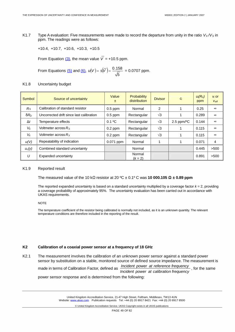
THE EXPRESSION OF UNCERTAINTY AND CONFIDENCE IN MEASUREMENT M3003 | EDITION 2 | JANUARY 2007
United Kingdom Accreditation Service, 21-47 High Street, Feltham, Middlesex, TW13 4UNWebsite: www.ukas.com Publication requests Tel: +44 (0) 20 8917 8421 Fax: +44 (0) 20 8917 8500
© United Kingdom Accreditation Service. UKAS Copyright exists in all UKAS publications
PAGE 49 OF 82
K1.7 Type A evaluation: Five measurements were made to record the departure from unity in the ratio VX /VS inppm. The readings were as follows:
+10.4, +10.7, +10.6, +10.3, +10.5
From Equation (3), the mean value V = +10.5 ppm.
From Equations (5) and (6), 5
158.0 VsVu = 0.0707 ppm.
K1.8 Uncertainty budget
Symbol Source of uncertaintyValue
±Probabilitydistribution Divisor ci
ui(RX)ppm
νi orνeff
RS Calibration of standard resistor 0.5 ppm Normal 2 1 0.25 ∞
δRD Uncorrected drift since last calibration 0.5 ppm Rectangular √3 1 0.289 ∞
Δt Temperature effects 0.1 ºC Rectangular √3 2.5 ppm/ºC 0.144 ∞
VS Voltmeter across RS 0.2 ppm Rectangular √3 1 0.115 ∞
VX Voltmeter across RX 0.2 ppm Rectangular √3 1 0.115 ∞
u(V) Repeatability of indication 0.071 ppm Normal 1 1 0.071 4
uc(y) Combined standard uncertainty Normal 0.445 >500
U Expanded uncertainty Normal(k = 2)
0.891 >500
K1.9 Reported result
The measured value of the 10 kΩresistor at 20 ºC ± 0.1º C was 10 000.105 Ω± 0.89 ppm
The reported expanded uncertainty is based on a standard uncertainty multiplied by a coverage factor k = 2, providinga coverage probability of approximately 95%. The uncertainty evaluation has been carried out in accordance withUKAS requirements.
NOTE
The temperature coefficient of the resistor being calibrated is normally not included, as it is an unknown quantity. The relevanttemperature conditions are therefore included in the reporting of the result.
K2 Calibration of a coaxial power sensor at a frequency of 18 GHz
K2.1 The measurement involves the calibration of an unknown power sensor against a standard powersensor by substitution on a stable, monitored source of defined source impedance. The measurement is
made in terms of Calibration Factor, defined asfrequencyncalibratioatpowerIncidentfrequencyreferenceatpowerIncident , for the same
power sensor response and is determined from the following:
THE EXPRESSION OF UNCERTAINTY AND CONFIDENCE IN MEASUREMENT M3003 | EDITION 2 | JANUARY 2007
United Kingdom Accreditation Service, 21-47 High Street, Feltham, Middlesex, TW13 4UNWebsite: www.ukas.com Publication requests Tel: +44 (0) 20 8917 8421 Fax: +44 (0) 20 8917 8500
© United Kingdom Accreditation Service. UKAS Copyright exists in all UKAS publications
PAGE 50 OF 82
Calibration Factor, KX = (KS + DS) x δDC x δM xδREF, where
KS = Calibration Factor of the standard sensor,DS = Drift in standard sensor since the previous calibration,δDC = Ratio of DC voltage outputs,δM = Ratio of Mismatch Losses,δREF = Ratio of reference power source (short-term stability of 50 MHz reference).
K2.2 Four separate measurements were made which involved disconnection and reconnection of both theunknown sensor and the standard sensor on a power transfer system. All measurements were made interms of voltage ratios that are proportional to calibration factor.
K2.3 None of the uncertainty contributions are considered to be correlated to any significant extent.
K2.4 There will be mismatch uncertainties associated with the source/standard sensor combination and withthe source/unknown sensor combination. These will be 200ΓGΓS% and 200ΓGΓX% respectively, where
ΓG = 0.02 at 50 MHz and 0.07 at 18 GHz,ΓS = 0.02 at 50 MHz and 0.10 at 18 GHz,ΓX = 0.02 at 50 MHz and 0.12 at 18 GHz.
These values include the uncertainty in the measurement of Γas described in paragraph E9.6.
K2.5 The standard power sensor was calibrated by an accredited laboratory 6 months before use; the expandeduncertainty of ± 1.1% was quoted for a coverage factor k = 2.
K2.6 The long-term stability of the standard sensor was estimated from the results of 5 annual calibrations. Nopredictable trend could be detected so drift corrections could not be made. The error due to secularstability was therefore assumed to be zero with limits, in this case, not greater than ± 0.4% per year. Avalue of ± 0.2% was used as the previous calibration was within 6 months.
K2.7 The instrumentation linearity uncertainty was estimated from measurements against a referenceattenuation standard. The expanded uncertainty for k = 2 of ± 0.1% applies to ratios up to 2:1.
K2.8 Type A evaluation: The four measurements resulted in the following values of Calibration Factor:
93.45% 92.20% 93.95% 93.02%
From Equation (3), the mean value XK = 93.16%.
From Equations (5) and (6), 4
7415.0 XR KsKu = 0.3707%.
THE EXPRESSION OF UNCERTAINTY AND CONFIDENCE IN MEASUREMENT M3003 | EDITION 2 | JANUARY 2007
United Kingdom Accreditation Service, 21-47 High Street, Feltham, Middlesex, TW13 4UNWebsite: www.ukas.com Publication requests Tel: +44 (0) 20 8917 8421 Fax: +44 (0) 20 8917 8500
© United Kingdom Accreditation Service. UKAS Copyright exists in all UKAS publications
PAGE 51 OF 82
K2.9 Uncertainty budget
Symbol Source of uncertainty Value± %
Probabilitydistribution
Divisor ciui(KX)
%νi orνeff
KS Calibration factor of standard 1.1 Normal 2.0 1.0 0.55 ∞DS Drift since last calibration 0.2 Rectangular √3 1.0 0.116 ∞δDC Instrumentation linearity 0.1 Normal 2.0 1.0 0.05 ∞δM Stability of 50 MHz reference 0.2 Rectangular √3 1.0 0.116 ∞
M1M2
M3M4
Mismatch:Standard sensor at 50 MHzUnknown sensor at 50 MHzStandard sensor at 18 GHzUnknown sensor at 18 GHz
0.080.081.401.68
U-shapedU-shapedU-shapedU-shaped
√2√2√2√2
1.01.01.01.0
0.060.060.991.19
∞∞∞∞
KR Repeatability of indication 0.37 Normal 1.0 1.0 0.37 3
u(KX) Combined standard uncertainty Normal 1.69 >500
U Expanded uncertainty Normal(k = 2) 3.39 >500
K2.10 Reported result
The measured calibration factor at 18 GHz was 93.2 % ± 3.4 %.
The reported expanded uncertainty is based on a standard uncertainty multiplied by a coverage factor k = 2, providinga coverage probability of approximately 95%. The uncertainty evaluation has been carried out in accordance withUKAS requirements.
NOTES
1 For the measurement of calibration factor, the uncertainty in the absolute value of the 50 MHz reference source need not beincluded if the standard and unknown sensors are calibrated using the same source, within the timescale allowed for its short-term stability.
2 This example illustrates the significance of mismatch uncertainty in measurements at relatively high frequencies.
3 In a subsequent use of a sensor further random components of uncertainty may arise due to the use of different connector pairs.
K3 Calibration of a 30 dB coaxial attenuator
K3.1 The measurement involves the calibration of a coaxial step attenuator at a frequency of 10 GHz using adual channel 30 MHz IF substitution measurement system. The measurement is made in terms of theattenuation in dB between a matched source and load from the following:
AX = Ab – Aa + AIF + DIF + LM + RD + M + AL + AR , where
Ab = Indicated attenuation with unknown attenuator set to zero,Aa = Indicated attenuation with unknown attenuator set to 30 dB,AIF = Calibration of reference IF attenuator,DIF = Drift in reference IF attenuator since last calibration,LM = Departure from linearity of mixer,RD = Error due to resolution of detection system,M = Mismatch error,AL = Effect of signal leakage,AR = Repeatability.

THE EXPRESSION OF UNCERTAINTY AND CONFIDENCE IN MEASUREMENT M3003 | EDITION 2 | JANUARY 2007
United Kingdom Accreditation Service, 21-47 High Street, Feltham, Middlesex, TW13 4UNWebsite: www.ukas.com Publication requests Tel: +44 (0) 20 8917 8421 Fax: +44 (0) 20 8917 8500
© United Kingdom Accreditation Service. UKAS Copyright exists in all UKAS publications
PAGE 52 OF 82
K3.2 The result is corrected for the calibrated value of the IF attenuator using the results from a calibrationcertificate, which gave an uncertainty of ± 0.005 dB at a coverage probability of 95% (k = 2).
K3.3 No correction is made for the drift of the IF attenuator. The limits of ± 0.002 dB were estimated from theresults of previous calibrations.
K3.4 No correction is made for mixer non-linearity. The uncertainty was estimated from a series of linearitymeasurements over the dynamic range of the system to be ± 0.002 dB/10dB. An uncertainty of ± 0.006 dBwas therefore assigned at 30 dB. The probability distribution is assumed to be rectangular.
K3.5 The resolution of the detection system was estimated to cause possible rounding errors of one-half of oneleast significant recorded digit i.e. ± 0.005 dB. This occurs twice - once for the 0 dB reference setting andagain for the 30 dB measurement. Two identical rectangular distributions with semi-range limits of acombine to give a triangular distribution with semi-range limits of 2a. The uncertainty due to resolution istherefore 0.01 dB with a triangular distribution.
K3.6 No correction is made for mismatch error. The mismatch uncertainty is calculated from the scatteringcoefficients using Equation E(5). The values used were as follows:
ΓL = 0.03 ΓG = 0.03 s11a = 0.05 s11b = 0.09 s22a = 0.05 s22b = 0.01 s21a = 1 s21b = 0.031
K3.7 Special experiments were performed to determine whether signal leakage had any significant effect onthe measurement system. No effect greater than ± 0.001 dB could be observed for attenuation values upto 70 dB. The probability distribution is assumed to be rectangular.
K3.8 Type A evaluation: Four measurements were made which involved setting the reference level with thestep attenuator set to zero and then measuring the attenuation for the 30 dB setting. The results were asfollows:
30.04 dB 30.07 dB 30.03 dB 30.06 dB
From Equation (3), the mean value XA = 30.050 dB.
From Equations (5) and (6), 4
018.0 XR AsAu = 0.009 dB.
K3.9 Uncertainty budget
Symbol Source of uncertainty Value± dB
Probabilitydistribution
Divisor ciui(AX)dB
νi orνeff
AIF Calibration of reference attenuator 0.005 Normal 2.0 1.0 0.0025 ∞
DIF Drift since last calibration 0.002 Rectangular √3 1.0 0.0016 ∞
LM Mixer non-linearity 0.006 Rectangular √3 1.0 0.0035 ∞
RD Resolution of indication 0.010 Triangular √6 1.0 0.0041 ∞
M Mismatch 0.022 Normal 1 1.0 0.022 ∞
AL Signal leakage effects 0.001 Rectangular √3 1.0 0.0006 ∞
AR Repeatability of indication 0.009 Normal 1.0 1.0 0.009 3
u(AX) Combined standard uncertainty Normal 0.0246 >500
U Expanded uncertainty Normal(k = 2) 0.0491 >500
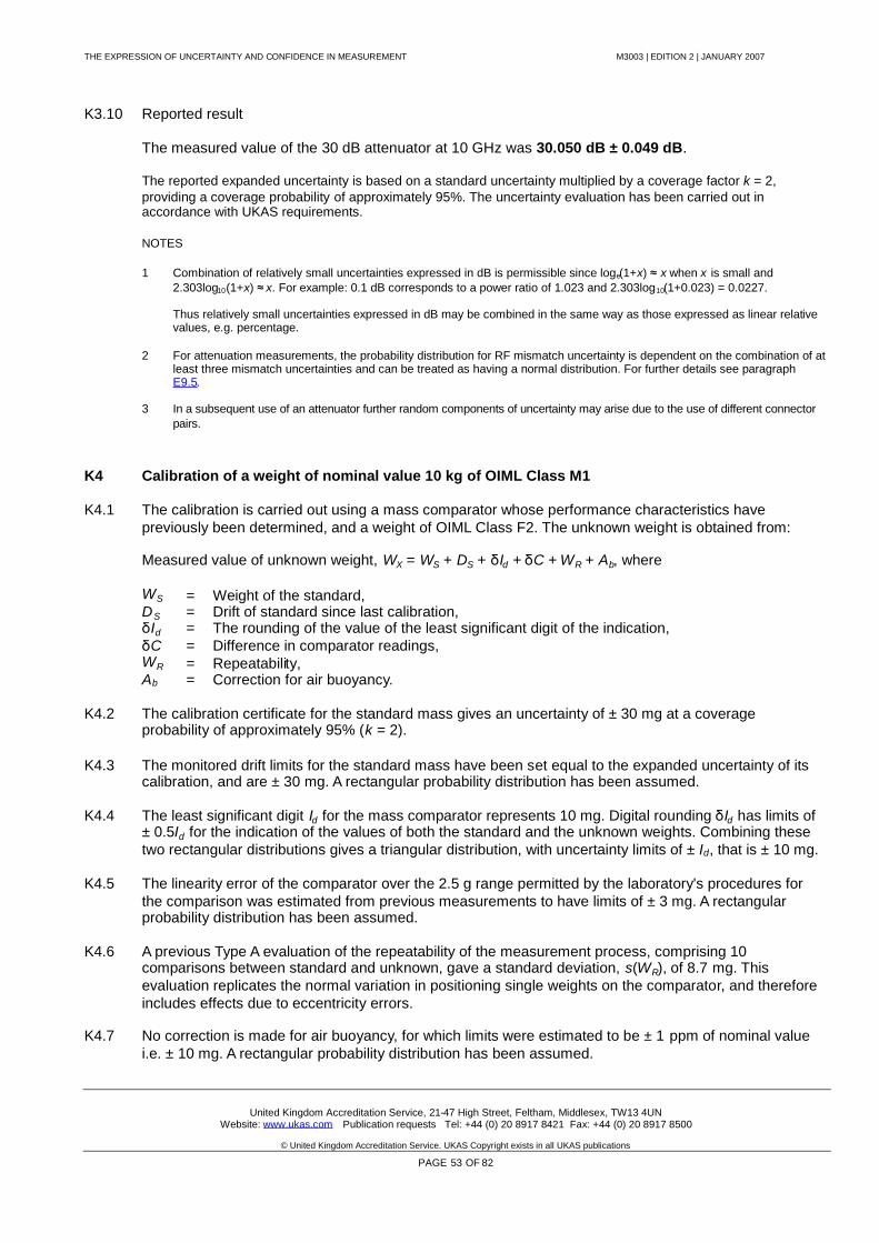
THE EXPRESSION OF UNCERTAINTY AND CONFIDENCE IN MEASUREMENT M3003 | EDITION 2 | JANUARY 2007
United Kingdom Accreditation Service, 21-47 High Street, Feltham, Middlesex, TW13 4UNWebsite: www.ukas.com Publication requests Tel: +44 (0) 20 8917 8421 Fax: +44 (0) 20 8917 8500
© United Kingdom Accreditation Service. UKAS Copyright exists in all UKAS publications
PAGE 53 OF 82
K3.10 Reported result
The measured value of the 30 dB attenuator at 10 GHz was 30.050 dB ± 0.049 dB.
The reported expanded uncertainty is based on a standard uncertainty multiplied by a coverage factor k = 2,providing a coverage probability of approximately 95%. The uncertainty evaluation has been carried out inaccordance with UKAS requirements.
NOTES
1 Combination of relatively small uncertainties expressed in dB is permissible since loge(1+x) ≈x when x is small and2.303log10(1+x) ≈x. For example: 0.1 dB corresponds to a power ratio of 1.023 and 2.303log10(1+0.023) = 0.0227.
Thus relatively small uncertainties expressed in dB may be combined in the same way as those expressed as linear relativevalues, e.g. percentage.
2 For attenuation measurements, the probability distribution for RF mismatch uncertainty is dependent on the combination of atleast three mismatch uncertainties and can be treated as having a normal distribution. For further details see paragraphE9.5.
3 In a subsequent use of an attenuator further random components of uncertainty may arise due to the use of different connectorpairs.
K4 Calibration of a weight of nominal value 10 kg of OIML Class M1
K4.1 The calibration is carried out using a mass comparator whose performance characteristics havepreviously been determined, and a weight of OIML Class F2. The unknown weight is obtained from:
Measured value of unknown weight, WX = WS + DS + δId + δC + WR + Ab, where
WS = Weight of the standard,DS = Drift of standard since last calibration,δId = The rounding of the value of the least significant digit of the indication,δC = Difference in comparator readings,WR = Repeatability,Ab = Correction for air buoyancy.
K4.2 The calibration certificate for the standard mass gives an uncertainty of ± 30 mg at a coverageprobability of approximately 95% (k = 2).
K4.3 The monitored drift limits for the standard mass have been set equal to the expanded uncertainty of itscalibration, and are ± 30 mg. A rectangular probability distribution has been assumed.
K4.4 The least significant digit Id for the mass comparator represents 10 mg. Digital rounding δId has limits of± 0.5Id for the indication of the values of both the standard and the unknown weights. Combining thesetwo rectangular distributions gives a triangular distribution, with uncertainty limits of ± Id, that is ± 10 mg.
K4.5 The linearity error of the comparator over the 2.5 g range permitted by the laboratory's procedures forthe comparison was estimated from previous measurements to have limits of ± 3 mg. A rectangularprobability distribution has been assumed.
K4.6 A previous Type A evaluation of the repeatability of the measurement process, comprising 10comparisons between standard and unknown, gave a standard deviation, s(WR), of 8.7 mg. Thisevaluation replicates the normal variation in positioning single weights on the comparator, and thereforeincludes effects due to eccentricity errors.
K4.7 No correction is made for air buoyancy, for which limits were estimated to be ± 1 ppm of nominal valuei.e. ± 10 mg. A rectangular probability distribution has been assumed.
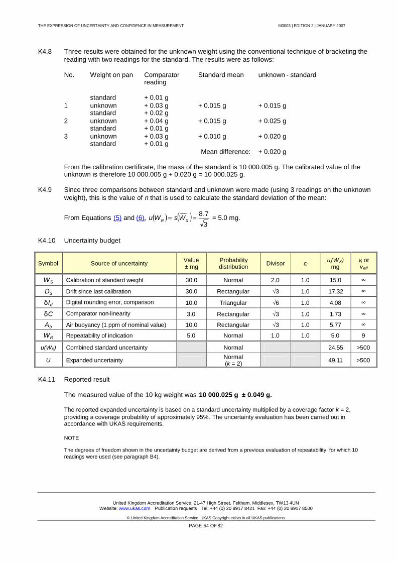
THE EXPRESSION OF UNCERTAINTY AND CONFIDENCE IN MEASUREMENT M3003 | EDITION 2 | JANUARY 2007
United Kingdom Accreditation Service, 21-47 High Street, Feltham, Middlesex, TW13 4UNWebsite: www.ukas.com Publication requests Tel: +44 (0) 20 8917 8421 Fax: +44 (0) 20 8917 8500
© United Kingdom Accreditation Service. UKAS Copyright exists in all UKAS publications
PAGE 54 OF 82
K4.8 Three results were obtained for the unknown weight using the conventional technique of bracketing thereading with two readings for the standard. The results were as follows:
No. Weight on pan Comparatorreading
Standard mean unknown - standard
standard + 0.01 g1 unknown + 0.03 g + 0.015 g + 0.015 g
standard + 0.02 g2 unknown + 0.04 g + 0.015 g + 0.025 g
standard + 0.01 g3 unknown + 0.03 g + 0.010 g + 0.020 g
standard + 0.01 gMean difference: + 0.020 g
From the calibration certificate, the mass of the standard is 10 000.005 g. The calibrated value of theunknown is therefore 10 000.005 g + 0.020 g = 10 000.025 g.
K4.9 Since three comparisons between standard and unknown were made (using 3 readings on the unknownweight), this is the value of n that is used to calculate the standard deviation of the mean:
From Equations (5) and (6), 3
7.8 XR WsWu = 5.0 mg.
K4.10 Uncertainty budget
Symbol Source of uncertainty Value± mg
Probabilitydistribution Divisor ci
ui(WX)mg
νi orνeff
WS Calibration of standard weight 30.0 Normal 2.0 1.0 15.0 ∞
DS Drift since last calibration 30.0 Rectangular √3 1.0 17.32 ∞
δId Digital rounding error, comparison 10.0 Triangular √6 1.0 4.08 ∞
δC Comparator non-linearity 3.0 Rectangular √3 1.0 1.73 ∞
Ab Air buoyancy (1 ppm of nominal value) 10.0 Rectangular √3 1.0 5.77 ∞
WR Repeatability of indication 5.0 Normal 1.0 1.0 5.0 9
u(WX) Combined standard uncertainty Normal 24.55 >500
U Expanded uncertainty Normal(k = 2) 49.11 >500
K4.11 Reported result
The measured value of the 10 kg weight was 10 000.025 g ± 0.049 g.
The reported expanded uncertainty is based on a standard uncertainty multiplied by a coverage factor k = 2,providing a coverage probability of approximately 95%. The uncertainty evaluation has been carried out inaccordance with UKAS requirements.
NOTE
The degrees of freedom shown in the uncertainty budget are derived from a previous evaluation of repeatability, for which 10readings were used (see paragraph B4).

THE EXPRESSION OF UNCERTAINTY AND CONFIDENCE IN MEASUREMENT M3003 | EDITION 2 | JANUARY 2007
United Kingdom Accreditation Service, 21-47 High Street, Feltham, Middlesex, TW13 4UNWebsite: www.ukas.com Publication requests Tel: +44 (0) 20 8917 8421 Fax: +44 (0) 20 8917 8500
© United Kingdom Accreditation Service. UKAS Copyright exists in all UKAS publications
PAGE 55 OF 82
K5 Calibration of a weighing machine of 205 g capacity by 0.1 mg digit
K5.1 The calibration is carried out using weights of OIML Class E2. Checks will normally be carried out forlinearity of response across the nominal capacity of the weighing machine, eccentricity effects of thepositioning of weights on the load receptor, and repeatability of the machine for repeated weighings nearfull load. The span of the weighing machine has been adjusted using its internal weight before calibration.The following uncertainty calculation is carried out for a near full loading of 200 g. The machine indicationsare obtained from
Unknown indication IX = WS + DS +δId0 + δId + Ab + IR , where
WS = Weight of the standard,DS = Drift of standard since last calibration,δId0 = The rounding of the value of one digit at the zero reading,δId = The rounding of the value of one digit of the indicated value,Ab = Correction for air buoyancy,IR = Repeatability of the indication.
K5.2 The calibration certificate for the stainless steel 200 g standard mass gives an uncertainty of ± 0.1 mg at acoverage probability of approximately 95% (k = 2).
K5.3 No correction is made for drift, but the calibration interval is set so as to limit the drift to ± 0.1 mg. Theprobability distribution is assumed to be rectangular.
K5.4 It is often the case that when a weighing machine is zeroed, or tared, it does so to a greater resolution thanthat provided by the digital readout. This can be thought of as an “internal digit” that is not presented to theuser. In this example, it is assumed that the “internal digit” size is one-tenth of that provided on the externaldisplay. The resulting possible rounding error is therefore ± 0.005 mg. The probability distribution isassumed to be rectangular.
NOTE
This is a good example of how a detailed knowledge of the principles of operation of a measuring instrument may berequired in order to identify and quantify the associated uncertainties.
K5.5 No correction can be made for the rounding due to the resolution of the digital display of the machine. Theleast significant digit on the range being calibrated corresponds to 0.1 mg and there is therefore a possiblerounding error of ± 0.05 mg. The probability distribution is assumed to be rectangular.
K5.6 No correction is made for air buoyancy. As the span of the machine was adjusted with its internal weightbefore calibration, the uncertainty limits were estimated to be ± 1 ppm of the nominal value, i.e. ± 0.2 mg.
K5.7 The repeatability of the machine was established from a series of 10 readings (Type A evaluation), whichgave a standard deviation, s (WR), of 0.05 mg. The degrees of freedom for this evaluation are 9, i.e. n - 1.
K5.8 Only one reading was taken to establish the weighing machine indication for each linearity and eccentricitypoint. For this calibration point the weighing machine indication, IX , was 199.9999 g when the 200 gstandard mass was applied. The value of n that is used to calculate the standard deviation of the mean ofthe indication, using the previously obtained repeatability standard deviation, s(WR), is therefore one:
From Equations (5) and (6), 105.0 XR WsIu = 0.05 mg.
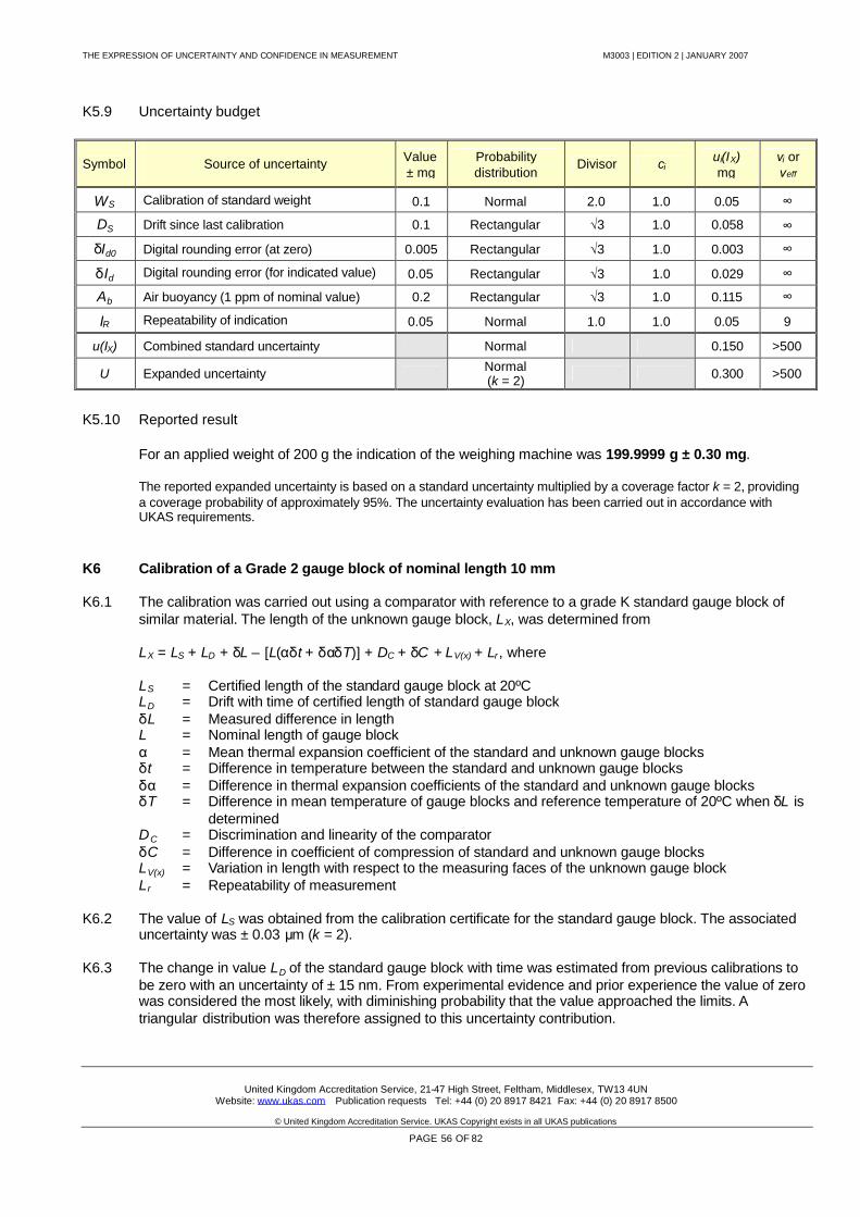
THE EXPRESSION OF UNCERTAINTY AND CONFIDENCE IN MEASUREMENT M3003 | EDITION 2 | JANUARY 2007
United Kingdom Accreditation Service, 21-47 High Street, Feltham, Middlesex, TW13 4UNWebsite: www.ukas.com Publication requests Tel: +44 (0) 20 8917 8421 Fax: +44 (0) 20 8917 8500
© United Kingdom Accreditation Service. UKAS Copyright exists in all UKAS publications
PAGE 56 OF 82
K5.9 Uncertainty budget
Symbol Source of uncertainty Value± mg
Probabilitydistribution
Divisor ciui(IX)mg
νi orνeff
WS Calibration of standard weight 0.1 Normal 2.0 1.0 0.05 ∞
DS Drift since last calibration 0.1 Rectangular √3 1.0 0.058 ∞
δId0 Digital rounding error (at zero) 0.005 Rectangular √3 1.0 0.003 ∞
δId Digital rounding error (for indicated value) 0.05 Rectangular √3 1.0 0.029 ∞
Ab Air buoyancy (1 ppm of nominal value) 0.2 Rectangular √3 1.0 0.115 ∞
IR Repeatability of indication 0.05 Normal 1.0 1.0 0.05 9
u(IX) Combined standard uncertainty Normal 0.150 >500
U Expanded uncertainty Normal(k = 2) 0.300 >500
K5.10 Reported result
For an applied weight of 200 g the indication of the weighing machine was 199.9999 g ± 0.30 mg.
The reported expanded uncertainty is based on a standard uncertainty multiplied by a coverage factor k = 2, providinga coverage probability of approximately 95%. The uncertainty evaluation has been carried out in accordance withUKAS requirements.
K6 Calibration of a Grade 2 gauge block of nominal length 10 mm
K6.1 The calibration was carried out using a comparator with reference to a grade K standard gauge block ofsimilar material. The length of the unknown gauge block, LX, was determined from
LX = LS + LD + δL – [L(αδt + δαδT)] + DC + δC + LV(x) + Lr , where
LS = Certified length of the standard gauge block at 20ºCLD = Drift with time of certified length of standard gauge blockδL = Measured difference in lengthL = Nominal length of gauge blockα = Mean thermal expansion coefficient of the standard and unknown gauge blocksδt = Difference in temperature between the standard and unknown gauge blocksδα = Difference in thermal expansion coefficients of the standard and unknown gauge blocksδT = Difference in mean temperature of gauge blocks and reference temperature of 20ºC when δL is
determinedDC = Discrimination and linearity of the comparatorδC = Difference in coefficient of compression of standard and unknown gauge blocksLV(x) = Variation in length with respect to the measuring faces of the unknown gauge blockLr = Repeatability of measurement
K6.2 The value of LS was obtained from the calibration certificate for the standard gauge block. The associateduncertainty was ± 0.03 μm (k = 2).
K6.3 The change in value LD of the standard gauge block with time was estimated from previous calibrations tobe zero with an uncertainty of ± 15 nm. From experimental evidence and prior experience the value of zerowas considered the most likely, with diminishing probability that the value approached the limits. Atriangular distribution was therefore assigned to this uncertainty contribution.
THE EXPRESSION OF UNCERTAINTY AND CONFIDENCE IN MEASUREMENT M3003 | EDITION 2 | JANUARY 2007
United Kingdom Accreditation Service, 21-47 High Street, Feltham, Middlesex, TW13 4UNWebsite: www.ukas.com Publication requests Tel: +44 (0) 20 8917 8421 Fax: +44 (0) 20 8917 8500
© United Kingdom Accreditation Service. UKAS Copyright exists in all UKAS publications
PAGE 57 OF 82
K6.4 The coefficient of thermal expansion applicable to each gauge block was assumed to have a value, α, of11.5 μm m-1 ºC-1 with limits of ± 1 μm m-1 ºC-1. Combining these two rectangular distributions, the differencein thermal expansion coefficient between the two blocks, δα, is ± 2 μm m-1 ºC-1 with a triangular distribution.For L = 10 mm this corresponds to ± 20 nm/ºC. This difference will have two influences:
(a) The difference in temperature, δt, between the standard and unknown gauge blocks was estimated to bezero with limits of ± 0.08 ºC, giving rise to a length uncertainty of ± 1.6 nm.
(b) The difference δT between the mean temperature of the two gauge blocks and the reference temperatureof 20 ºC was measured and was assigned limits of ± 0.2 ºC, giving rise to a length uncertainty of ± 4 nm.
As the influence of δαappears directly in both these uncertainty contributions they are considered to becorrelated and, in accordance with paragraph D3.3, the corresponding uncertainties have been addedbefore being combined with the remaining contributions. This is included in the uncertainty budget as δTs,x.
K6.5 The error due to the discrimination and non-linearity of the comparator, DC, was taken as zero with limits of± 0.05 μm, assessed from previous measurements. Similarly, the difference in elastic compression δCbetween the standard and unknown gauge blocks was estimated to be zero with limits of ± 0.005 μm.
K6.6 The variation in length of the unknown gauge block, LV(x), was considered to comprise two components:(i) Effect due to incorrect central alignment of the probe; assuming this misalignment was within a circle ofradius 0.5 mm, calculations based on the specifications for grade C gauge blocks indicted an uncertainty of± 17 nm. (ii) Effects due to surface irregularities such as scratches or indentations; such effects have adetection limit of approximately 25 nm when examined by experienced staff. Quadrature combination ofthese contributions gives an uncertainty due to surface irregularities of ± 30 nm. As this is the combinationof two rectangular distributions, of similar magnitude, the resulting distribution was assumed to betriangular.
K6.7 The repeatability of the calibration process was established from previous measurements using gaugeblocks of similar type and nominal length. This Type A evaluation, based upon 11 measurements and usingEquation (7), yielded a standard deviation s(LR) of 16 nm.
K6.8 The calibration of the unknown gauge block was established from a single measurement; however, as theconditions were the same as for the previous evaluation of repeatability the standard uncertainty due torepeatability can be obtained from this previous value of standard deviation, with n = 1, because only onereading is made for the actual calibration.
From Equation (6), 1
16 XR LsLu = 16 nm.
The measured length of the unknown gauge block was 9.999 94 mm.

THE EXPRESSION OF UNCERTAINTY AND CONFIDENCE IN MEASUREMENT M3003 | EDITION 2 | JANUARY 2007
United Kingdom Accreditation Service, 21-47 High Street, Feltham, Middlesex, TW13 4UNWebsite: www.ukas.com Publication requests Tel: +44 (0) 20 8917 8421 Fax: +44 (0) 20 8917 8500
© United Kingdom Accreditation Service. UKAS Copyright exists in all UKAS publications
PAGE 58 OF 82
K6.9 Uncertainty budget
Symbol Source of uncertainty Value± nm
Probabilitydistribution Divisor ci
ui(LX)nm
νi orνeff
LS Calibration of the standard gauge block 30 Normal 2.0 1.0 15.0 ∞LD Drift since last calibration 15 Triangular √6 1.0 6.1 ∞
DC Comparator 50 Rectangular √3 1.0 28.9 ∞
δC Difference in elastic compression 5.0 Rectangular √3 1.0 2.9 ∞
δTs,x Temperature effects 5.6 Triangular √6 1.0 2.3 ∞
LV(x) Length variation of unknown gauge block 30 Triangular √6 1.0 12.3 ∞Lr Repeatability 16 Normal 1.0 1.0 16.0 10
u(LX) Combined standard uncertainty Normal 39.0 >400
U Expanded uncertainty Normal(k = 2) 77.9 >400
K6.10 Reported result
The measured length of the gauge block was 9.999 94 mm ± 0.078 μm.
The reported expanded uncertainty is based on a standard uncertainty multiplied by a coverage factor k = 2,providing a coverage probability of approximately 95%. The uncertainty evaluation has been carried out inaccordance with UKAS requirements.
K7 Calibration of a Type N thermocouple at 1000ºC
K7.1 A Type N thermocouple is calibrated against two reference standard Type R thermocouples in ahorizontal furnace at a temperature of 1000ºC. The emfs generated by the thermocouples are measuredusing a digital microvoltmeter via a selector/reversing switch. All the thermocouples have their referencejunctions at 0ºC. The unknown thermocouple is connected to the reference point using compensatingcables.
K7.2 The temperature tx of the hot junction of the unknown thermocouple is given by
FDS
SRiSiSiSsx tt
Ct
VVVVtt δδδ
δδδ
0
021
FDSS
sRsiSsiSsiSs ttt
CCVCVCVCVt δδδδδδ 0
021
The voltage Vx(t) across the thermocouple wires with the reference junction at 0 ºC during the calibrationis
0
021
0
0
X
X
XRTHiXiXiX
X
X
xxxx C
tC
tVhVVVCt
CttVtV
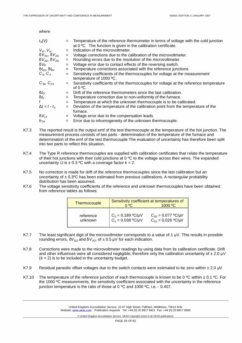
THE EXPRESSION OF UNCERTAINTY AND CONFIDENCE IN MEASUREMENT M3003 | EDITION 2 | JANUARY 2007
United Kingdom Accreditation Service, 21-47 High Street, Feltham, Middlesex, TW13 4UNWebsite: www.ukas.com Publication requests Tel: +44 (0) 20 8917 8421 Fax: +44 (0) 20 8917 8500
© United Kingdom Accreditation Service. UKAS Copyright exists in all UKAS publications
PAGE 59 OF 82
where
tS(V) = Temperature of the reference thermometer in terms of voltage with the cold junctionat 0 ºC. The function is given in the calibration certificate.
ViS, ViX = Indication of the microvoltmeter.δViS1, δViX1 = Voltage corrections due to the calibration of the microvoltmeter.δViS2, δViX2 = Rounding errors due to the resolution of the microvoltmeter.δVR = Voltage error due to contact effects of the reversing switch.δt0S, δt0X = Temperature corrections associated with the reference junctions.CS, CX = Sensitivity coefficients of the thermocouples for voltage at the measurement
temperature of 1000 ºC.CS0, CX0 = Sensitivity coefficients of the thermocouples for voltage at the reference temperature
of 0 ºC.δtD = Drift of the reference thermometers since the last calibration.δtF = Temperature correction due to non-uniformity of the furnace.t = Temperature at which the unknown thermocouple is to be calibrated.Δt = t - tX = Deviation of the temperature of the calibration point from the temperature of the
furnace.δVLX = Voltage error due to the compensation leads.hTH = Error due to inhomogeneity of the unknown thermocouple.
K7.3 The reported result is the output emf of the test thermocouple at the temperature of the hot junction. Themeasurement process consists of two parts - determination of the temperature of the furnace anddetermination of the emf of the test thermocouple The evaluation of uncertainty has therefore been splitinto two parts to reflect this situation.
K7.4 The Type R reference thermocouples are supplied with calibration certificates that relate the temperatureof their hot junctions with their cold junctions at 0 ºC to the voltage across their wires. The expandeduncertainty U is ± 0.3 ºC with a coverage factor k = 2.
K7.5 No correction is made for drift of the reference thermocouples since the last calibration but anuncertainty of ± 0.3ºC has been estimated from previous calibrations. A rectangular probabilitydistribution has been assumed.
K7.6 The voltage sensitivity coefficients of the reference and unknown thermocouples have been obtainedfrom reference tables as follows:
Sensitivity coefficient at temperatures ofThermocouple 0 ºC 1000 ºC
reference CS = 0.189 ºC/μV CS0 = 0.077 ºC/μVunknown CX = 0.038 ºC/μV CX0 = 0.026 ºC/μV
K7.7 The least significant digit of the microvoltmeter corresponds to a value of 1 μV. This results in possiblerounding errors, δViS2 and δViX2, of ± 0.5 μV for each indication.
K7.8 Corrections were made to the microvoltmeter readings by using data from its calibration certificate. Driftand other influences were all considered negligible, therefore only the calibration uncertainty of ± 2.0 μV(k = 2) is to be included in the uncertainty budget.
K7.9 Residual parasitic offset voltages due to the switch contacts were estimated to be zero within ± 2.0 μV.
K7.10 The temperature of the reference junction of each thermocouple is known to be 0 ºC within ± 0.1 ºC. Forthe 1000 ºC measurements, the sensitivity coefficient associated with the uncertainty in the referencejunction temperature is the ratio of those at 0 ºC and 1000 ºC, i.e. - 0.407.

THE EXPRESSION OF UNCERTAINTY AND CONFIDENCE IN MEASUREMENT M3003 | EDITION 2 | JANUARY 2007
United Kingdom Accreditation Service, 21-47 High Street, Feltham, Middlesex, TW13 4UNWebsite: www.ukas.com Publication requests Tel: +44 (0) 20 8917 8421 Fax: +44 (0) 20 8917 8500
© United Kingdom Accreditation Service. UKAS Copyright exists in all UKAS publications
PAGE 60 OF 82
K7.11 The temperature gradients inside the furnace had been measured. At 1000 ºC deviations from non-uniformity of temperature in the region of measurement are within ± 1 ºC
K7.12 The compensation leads had been tested in the range 0 ºC to 40 ºC. Voltage differences between theleads and the thermocouple wires were estimated to be less than ± 5 μV.
K7.13 The error due to inhomogeneity of the unknown thermocouple was determined during the calibration byvarying the immersion depth. Corrections are not practical for this effect therefore the error wasassumed to be zero within ± 0.3 ºC.
K7.14 The sequence of measurements is as follows: 1 First standard thermocouple2 Unknown thermocouple3 Second standard thermocouple4 Unknown thermocouple5 First standard thermocouple
The polarity is then reversed and the sequence is repeated. Four readings are thus obtained for all thethermocouples. This sequence reduces the effects of drift in the thermal source and parasiticthermocouple voltages. The results were as follows:
Thermocouple: First standard Unknown Second standard
Corrected voltages: + 10500 μV+ 10503 μV– 10503 μV– 10504 μV
+ 36245 μV+ 36248 μV– 36248 μV– 36251 μV
+ 10503 μV+ 10503 μV– 10505 μV– 10505 μV
Absolute mean values: 10502.5 μV 36248 μV 10504.0 μV
Temperature of hot junctions: 1000.4 ºC 1000.6 ºC
Mean temperature of furnace: 1000.6 ºC
K7.15 The thermocouple output emf is corrected for the difference between the nominal temperature of 1000ºC and the measured temperature of 1000.5 ºC. The reported thermocouple output is
5.1000100036248XV µV = 36230 μV.
K7.16 In this example it is assumed that the procedure requires that the difference between the two standardsmust not exceed 0.3 ºC. If this is the case then the measurement must be repeated and/or the reasonfor the difference investigated.
K7.17 From the four readings on each thermocouple, one observation of the mean voltage of each thermocouplewas deduced. The mean voltages of the reference thermocouples are converted to temperatureobservations by means of temperature/voltage relationships given in their calibration certificates. Thesetemperature values are highly correlated. By taking the mean they are combined into one observation ofthe temperature of the furnace at the location of the test thermocouple. In a similar way one observation ofthe voltage of the test thermocouple is extracted.
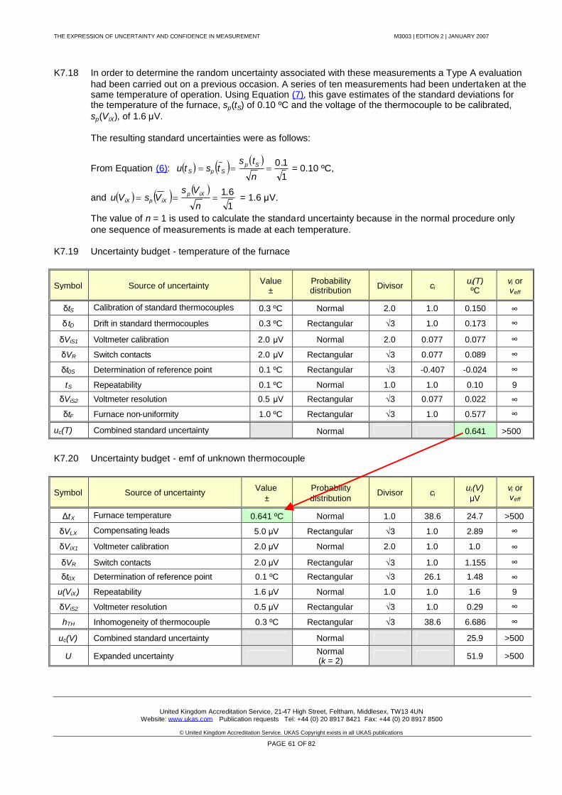
THE EXPRESSION OF UNCERTAINTY AND CONFIDENCE IN MEASUREMENT M3003 | EDITION 2 | JANUARY 2007
United Kingdom Accreditation Service, 21-47 High Street, Feltham, Middlesex, TW13 4UNWebsite: www.ukas.com Publication requests Tel: +44 (0) 20 8917 8421 Fax: +44 (0) 20 8917 8500
© United Kingdom Accreditation Service. UKAS Copyright exists in all UKAS publications
PAGE 61 OF 82
K7.18 In order to determine the random uncertainty associated with these measurements a Type A evaluationhad been carried out on a previous occasion. A series of ten measurements had been undertaken at thesame temperature of operation. Using Equation (7), this gave estimates of the standard deviations forthe temperature of the furnace, sp(tS) of 0.10 ºC and the voltage of the thermocouple to be calibrated,sp(ViX), of 1.6 μV.
The resulting standard uncertainties were as follows:
From Equation (6): 11.0
n
tststu Sp
SpS = 0.10 ºC,
and 16.1
n
VsVsVu iXp
iXpiX = 1.6 μV.
The value of n = 1 is used to calculate the standard uncertainty because in the normal procedure onlyone sequence of measurements is made at each temperature.
K7.19 Uncertainty budget - temperature of the furnace
Symbol Source of uncertainty Value±
Probabilitydistribution Divisor ci
ui(T)ºC
νi orνeff
δtS Calibration of standard thermocouples 0.3 ºC Normal 2.0 1.0 0.150 ∞δtD Drift in standard thermocouples 0.3 ºC Rectangular √3 1.0 0.173 ∞
δViS1 Voltmeter calibration 2.0 μV Normal 2.0 0.077 0.077 ∞
δVR Switch contacts 2.0 μV Rectangular √3 0.077 0.089 ∞
δt0S Determination of reference point 0.1 ºC Rectangular √3 -0.407 -0.024 ∞
tS Repeatability 0.1 ºC Normal 1.0 1.0 0.10 9
δViS2 Voltmeter resolution 0.5 μV Rectangular √3 0.077 0.022 ∞δtF Furnace non-uniformity 1.0 ºC Rectangular √3 1.0 0.577 ∞
uc(T) Combined standard uncertainty Normal 0.641 >500
K7.20 Uncertainty budget - emf of unknown thermocouple
Symbol Source of uncertainty Value±
Probabilitydistribution
Divisor ciui(V)μV
νi orνeff
ΔtX Furnace temperature 0.641 ºC Normal 1.0 38.6 24.7 >500
δVLX Compensating leads 5.0 μV Rectangular √3 1.0 2.89 ∞
δViX1 Voltmeter calibration 2.0 μV Normal 2.0 1.0 1.0 ∞
δVR Switch contacts 2.0 μV Rectangular √3 1.0 1.155 ∞δt0X Determination of reference point 0.1 ºC Rectangular √3 26.1 1.48 ∞
u(ViX) Repeatability 1.6 μV Normal 1.0 1.0 1.6 9
δViS2 Voltmeter resolution 0.5 μV Rectangular √3 1.0 0.29 ∞
hTH Inhomogeneity of thermocouple 0.3 ºC Rectangular √3 38.6 6.686 ∞
uc(V) Combined standard uncertainty Normal 25.9 >500
U Expanded uncertainty Normal(k = 2) 51.9 >500
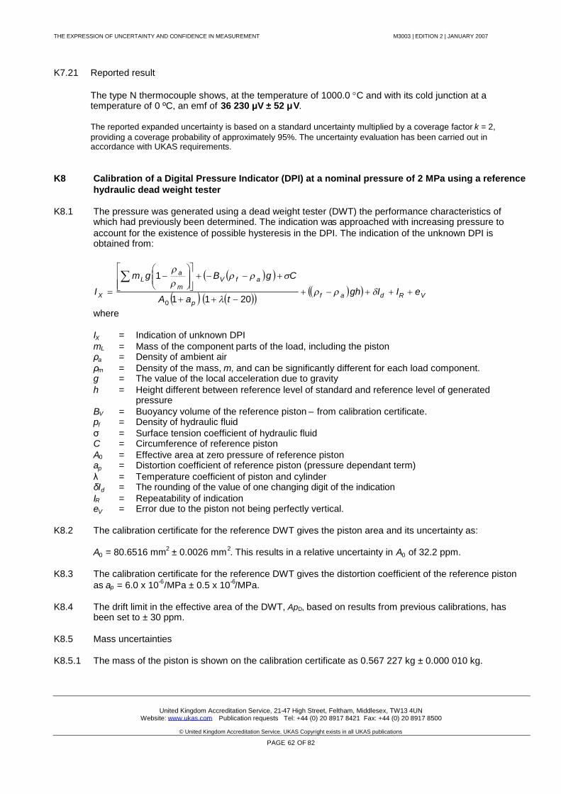
THE EXPRESSION OF UNCERTAINTY AND CONFIDENCE IN MEASUREMENT M3003 | EDITION 2 | JANUARY 2007
United Kingdom Accreditation Service, 21-47 High Street, Feltham, Middlesex, TW13 4UNWebsite: www.ukas.com Publication requests Tel: +44 (0) 20 8917 8421 Fax: +44 (0) 20 8917 8500
© United Kingdom Accreditation Service. UKAS Copyright exists in all UKAS publications
PAGE 62 OF 82
K7.21 Reported result
The type N thermocouple shows, at the temperature of 1000.0 C and with its cold junction at atemperature of 0 ºC, an emf of 36 230 μV ± 52 μV.
The reported expanded uncertainty is based on a standard uncertainty multiplied by a coverage factor k = 2,providing a coverage probability of approximately 95%. The uncertainty evaluation has been carried out inaccordance with UKAS requirements.
K8 Calibration of a Digital Pressure Indicator (DPI) at a nominal pressure of 2 MPa using a referencehydraulic dead weight tester
K8.1 The pressure was generated using a dead weight tester (DWT) the performance characteristics ofwhich had previously been determined. The indication was approached with increasing pressure toaccount for the existence of possible hysteresis in the DPI. The indication of the unknown DPI isobtained from:
VRdafp
afVm
aL
X eIIghtaA
CgBgm
I
2011
1
0
where
IX = Indication of unknown DPImL = Mass of the component parts of the load, including the pistonρa = Density of ambient airρm = Density of the mass, m, and can be significantly different for each load component.g = The value of the local acceleration due to gravityh = Height different between reference level of standard and reference level of generated
pressureBV = Buoyancy volume of the reference piston – from calibration certificate.pf = Density of hydraulic fluidσ = Surface tension coefficient of hydraulic fluidC = Circumference of reference pistonA0 = Effective area at zero pressure of reference pistonap = Distortion coefficient of reference piston (pressure dependant term)λ = Temperature coefficient of piston and cylinderδId = The rounding of the value of one changing digit of the indicationIR = Repeatability of indicationeV = Error due to the piston not being perfectly vertical.
K8.2 The calibration certificate for the reference DWT gives the piston area and its uncertainty as:
A0 = 80.6516 mm2 ± 0.0026 mm2. This results in a relative uncertainty in A0 of 32.2 ppm.
K8.3 The calibration certificate for the reference DWT gives the distortion coefficient of the reference pistonas ap = 6.0 x 10⁻⁶/MPa ± 0.5 x 10⁻⁶/MPa.
K8.4 The drift limit in the effective area of the DWT, ApD, based on results from previous calibrations, hasbeen set to ± 30 ppm.
K8.5 Mass uncertainties
K8.5.1 The mass of the piston is shown on the calibration certificate as 0.567 227 kg ± 0.000 010 kg.
THE EXPRESSION OF UNCERTAINTY AND CONFIDENCE IN MEASUREMENT M3003 | EDITION 2 | JANUARY 2007
United Kingdom Accreditation Service, 21-47 High Street, Feltham, Middlesex, TW13 4UNWebsite: www.ukas.com Publication requests Tel: +44 (0) 20 8917 8421 Fax: +44 (0) 20 8917 8500
© United Kingdom Accreditation Service. UKAS Copyright exists in all UKAS publications
PAGE 63 OF 82
K8.5.2 The drift of the piston mass, based on previous calibrations, has been set to 0.000 015 kg.
K8.5.3 The uncertainty of the mass set is shown on the calibration certificate for the three weights “A”, “B” and“C” used to generate 2 MPa as:
A = 0.255 242 kg ± 0.000 010 kgB = 7.402 137 kg ± 0.000 050 kgC = 8.224 784 kg ± 0.000 050 kg
K8.5.4 The limits to the drift of the mass set have been set to be equal to the expanded uncertainty of itscalibration, i.e. 10 mg, 50 mg and 50 mg respectively.
K8.5.5 To obtain the combined mass uncertainty, u(m), in relative terms:
Relative uncertainty in mass u(m) =(kg)CBAPistonofMass
(mg)CBAPistonofyUncertaint
ppm
=784224.8137402.7242255.0227567.0
50501010
= 7.30 ppm
Similarly, for drift this gives mD = 7.60 ppm.
K8.6 The uncertainty in the temperature of the piston, ut, coming from the analysis of the temperature indictorused has been set as ± 0.5ºC. This will affect the pressure generated in proportion to the temperaturecoefficient of the piston and cylinder combination. In this case a steel piston and cylinder has atemperature coefficient of 23 ppm/ºC. This figure was obtained from the calibration certificate for theDWT.
K8.7 A correction had been made for the value of the local acceleration due to gravity. This value had beenestimated from knowledge of the measurement location and took the Bouguer anomalies into account.The expanded uncertainty associated with this estimate, Ug, was ± 3 ppm (k = 2).
K8.8 No correction has been made for air buoyancy therefore, as all masses have an assumed density of7800 kgm-3, the uncertainty, ab, is estimated to be ± 13 ppm.
K8.9 The uncertainty relating to fluid head effects, fh, arises from the height different between the referencelevel of the reference DWT and the generated pressure datum point. It is estimated as +2 mm and theuncertainty in this estimate is ± 1 mm. No correction is made therefore a limit value of ± 3 mm has beenassigned for the uncertainty associated with fluid head effects. Assuming that the density of the oil usedis 917 kg/m3 and the local value of g is 9.81 ms-2, then the uncertainty associated with the fluid headeffect is 917 x 9.81 x 0.003 = 27.0 Pa. In relative terms this corresponds to an uncertainty of ± 13.5 ppmat 2 MPa.
K8.10 The uncertainty contribution, fe, from buoyancy volume, surface tension and fluid density effects hasbeen estimated as ± 2 ppm based on a relative uncertainty in each of ± 10%.
K8.11 The repeatability of the calibration process had been established from previous measurements using DPIsof similar type and nominal range. This Type A evaluation, based upon 10 measurements and usingEquation (7), yielded a relative standard deviation s(PR) of 16 ppm.
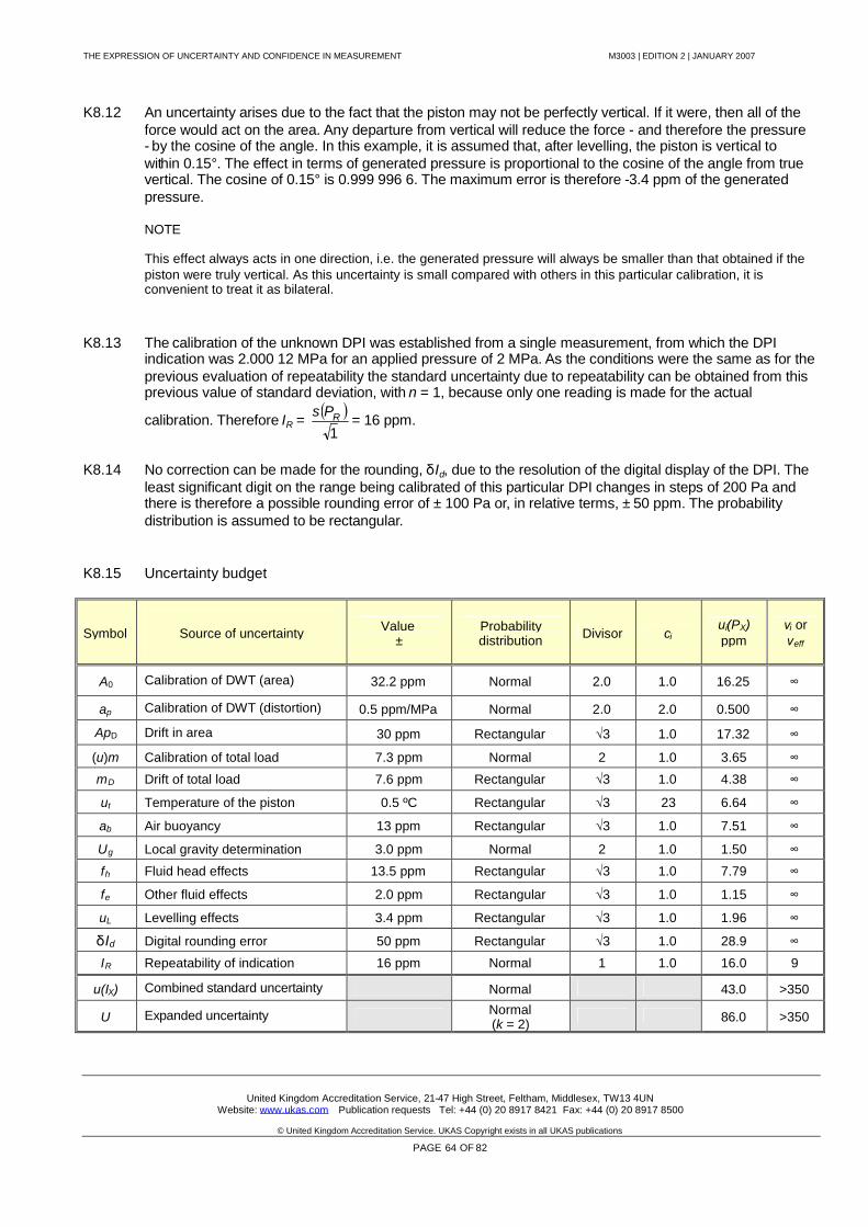
THE EXPRESSION OF UNCERTAINTY AND CONFIDENCE IN MEASUREMENT M3003 | EDITION 2 | JANUARY 2007
United Kingdom Accreditation Service, 21-47 High Street, Feltham, Middlesex, TW13 4UNWebsite: www.ukas.com Publication requests Tel: +44 (0) 20 8917 8421 Fax: +44 (0) 20 8917 8500
© United Kingdom Accreditation Service. UKAS Copyright exists in all UKAS publications
PAGE 64 OF 82
K8.12 An uncertainty arises due to the fact that the piston may not be perfectly vertical. If it were, then all of theforce would act on the area. Any departure from vertical will reduce the force - and therefore the pressure- by the cosine of the angle. In this example, it is assumed that, after levelling, the piston is vertical towithin 0.15°. The effect in terms of generated pressure is proportional to the cosine of the angle from truevertical. The cosine of 0.15° is 0.999 996 6. The maximum error is therefore -3.4 ppm of the generatedpressure.
NOTE
This effect always acts in one direction, i.e. the generated pressure will always be smaller than that obtained if thepiston were truly vertical. As this uncertainty is small compared with others in this particular calibration, it isconvenient to treat it as bilateral.
K8.13 The calibration of the unknown DPI was established from a single measurement, from which the DPIindication was 2.000 12 MPa for an applied pressure of 2 MPa. As the conditions were the same as for theprevious evaluation of repeatability the standard uncertainty due to repeatability can be obtained from thisprevious value of standard deviation, with n = 1, because only one reading is made for the actual
calibration. Therefore IR = 1RPs = 16 ppm.
K8.14 No correction can be made for the rounding, δId, due to the resolution of the digital display of the DPI. Theleast significant digit on the range being calibrated of this particular DPI changes in steps of 200 Pa andthere is therefore a possible rounding error of ± 100 Pa or, in relative terms, ± 50 ppm. The probabilitydistribution is assumed to be rectangular.
K8.15 Uncertainty budget
Symbol Source of uncertainty Value±
Probabilitydistribution Divisor ci
ui(PX)ppm
νi orνeff
A0 Calibration of DWT (area) 32.2 ppm Normal 2.0 1.0 16.25 ∞
ap Calibration of DWT (distortion) 0.5 ppm/MPa Normal 2.0 2.0 0.500 ∞
ApD Drift in area 30 ppm Rectangular √3 1.0 17.32 ∞
(u)m Calibration of total load 7.3 ppm Normal 2 1.0 3.65 ∞
mD Drift of total load 7.6 ppm Rectangular √3 1.0 4.38 ∞
ut Temperature of the piston 0.5 ºC Rectangular √3 23 6.64 ∞
ab Air buoyancy 13 ppm Rectangular √3 1.0 7.51 ∞
Ug Local gravity determination 3.0 ppm Normal 2 1.0 1.50 ∞
fh Fluid head effects 13.5 ppm Rectangular √3 1.0 7.79 ∞
fe Other fluid effects 2.0 ppm Rectangular √3 1.0 1.15 ∞
uL Levelling effects 3.4 ppm Rectangular √3 1.0 1.96 ∞
δId Digital rounding error 50 ppm Rectangular √3 1.0 28.9 ∞
IR Repeatability of indication 16 ppm Normal 1 1.0 16.0 9
u(IX) Combined standard uncertainty Normal 43.0 >350
U Expanded uncertainty Normal(k = 2) 86.0 >350
THE EXPRESSION OF UNCERTAINTY AND CONFIDENCE IN MEASUREMENT M3003 | EDITION 2 | JANUARY 2007
United Kingdom Accreditation Service, 21-47 High Street, Feltham, Middlesex, TW13 4UNWebsite: www.ukas.com Publication requests Tel: +44 (0) 20 8917 8421 Fax: +44 (0) 20 8917 8500
© United Kingdom Accreditation Service. UKAS Copyright exists in all UKAS publications
PAGE 65 OF 82
K8.16 The generated pressure was calculated from the mass of the piston (K8.5.1), that of the mass set(K8.5.3) and the following quantities:
Temperature of Piston: 21 ºCBuoyancy volume of piston: 3.10-7 m3
Air density: 1.2 kg/m3
Local gravity: 9.811812 ms-2
Oil surface tension coefficient: 0.0315 N/m
This results in an applied pressure of 2.000 806 MPa.
K8.17 Reported result
The pressure was applied in an increasing direction until it reached a final value of 2.000 806 MPa. Theindication of the digital pressure indicator was 2.000 84 MPa ± 86 ppm.
The reported expanded uncertainty is based on a standard uncertainty multiplied by a coverage factor k = 2,providing a coverage probability of approximately 95%. The uncertainty evaluation has been carried out inaccordance with UKAS requirements.
NOTES
1 In this example, the uncertainty due to resolution, δId, is larger than any other contribution and is assigned a rectangulardistribution. Nevertheless, the combined standard uncertainty is still Gaussian, due to the presence of the other uncertainties,even though they are of smaller magnitude. This has been verified by Monte Carlo Simulation techniques.
2 The resolution uncertainty is based on the least significant digit of the DPI. However, this changes in steps of 2 digits for thisparticular DPI, therefore the digital rounding error is 1 digit.
3 This uncertainty budget has been constructed in relative terms (ppm), as most of the errors that arise are proportional to thegenerated pressure and it is the convention in this particular field of measurement to express uncertainties in this manner. If itis required that the uncertainty is reported in absolute units, it can be calculated from the reported value and the relativeuncertainty. In this case, the expanded uncertainty in absolute terms is ± 0.000 17 MPa.
THE EXPRESSION OF UNCERTAINTY AND CONFIDENCE IN MEASUREMENT M3003 | EDITION 2 | JANUARY 2007
United Kingdom Accreditation Service, 21-47 High Street, Feltham, Middlesex, TW13 4UNWebsite: www.ukas.com Publication requests Tel: +44 (0) 20 8917 8421 Fax: +44 (0) 20 8917 8500
© United Kingdom Accreditation Service. UKAS Copyright exists in all UKAS publications
PAGE 66 OF 82
APPENDIX LEXPRESSION OF UNCERTAINTY FOR A RANGE OF VALUES
L1 Introduction
L1.1 On occasions it is convenient to provide a statement of uncertainty that describes a range of valuesrather than a single result.
L1.2 The GUM deals with expression of uncertainties for the reporting of a single value of a measurand, ormore than one parameter derived from the same set of data. In practice many measuring instrumentsare calibrated at several points on a range and the use of an expression describing the uncertainty atany of these points can be desirable.
L1.3 This Appendix therefore describes the situations when this can occur, explains how it can be dealt withusing the principles of this code of practice and provides an illustration of the process using a workedexample.
L2 Principles
L2.1 When measurements are made over a range of values and the corresponding sources of uncertainty areexamined it may be found that some are absolute in nature (i.e. they arise in a manner that isindependent of the value of the measurand) and some are relative in nature (i.e. they arise in a mannerthat makes them proportional to the value of the measurand).
L2.2 It is possible, of course, to calculate a value for the expanded uncertainty for each reported value overthe range. This can give problems when reporting values near zero as a relative term may not beappropriate and an absolute term has to be used. Conversely, when reporting values higher up the scaleit may be desirable to express the uncertainty in relative terms, as this is often how instrumentspecifications are expressed.
L2.3 If the instrument being calibrated is subsequently to be used in a situation where a further analysis ofuncertainty is required, the user may also require to express these uncertainties in both absolute andrelative terms. However if the user has only been provided with a single value of uncertainty for eachreported value, it would not be possible to extract the absolute and relative parts from these singlevalues. Reporting uncertainties in both absolute and relative terms therefore provides more informationto the user than if a series of single values are quoted. Additionally, it is often more representative of theway instrument specifications are expressed.
L2.4 The process of calculating a value of expanded uncertainty describing a range of values is identical tothat for single values except that the absolute and relative terms are identified as such and, in effect, aseparate uncertainty evaluation is carried out for each. These evaluations are carried out in the manneralready described in this publication.
L2.5 The results of these evaluations are then expressed as separate absolute and relative terms.Traditionally this has been expressed in the form
± (UREL + UABS)
This linear addition of quantities is not in accordance with the principles embodied in the GUM, unlessthere happens to be a high degree of correlation between the absolute and relative terms - which is notusually the case. The two values should normally be reported separately with an appropriate statementdescribing how they should be combined. A suggested statement is given in the example in L3.13.
THE EXPRESSION OF UNCERTAINTY AND CONFIDENCE IN MEASUREMENT M3003 | EDITION 2 | JANUARY 2007
United Kingdom Accreditation Service, 21-47 High Street, Feltham, Middlesex, TW13 4UNWebsite: www.ukas.com Publication requests Tel: +44 (0) 20 8917 8421 Fax: +44 (0) 20 8917 8500
© United Kingdom Accreditation Service. UKAS Copyright exists in all UKAS publications
PAGE 67 OF 82
L3 Example of uncertainty evaluation for a range of values
L3.1 In this example a 6½-digit electronic multimeter is calibrated on its 1 V dc range using a multi-functioncalibrator.
L3.2 The calibrations were carried out in both polarities at 0.1 V increments from zero to 1 V and additionallyat 1.5 V and 1.9 V. Only one measurement was carried out at each point and therefore reliance wasplaced on a previous evaluation of repeatability using similar multimeters.
L3.3 No corrections were made for known errors of the calibrator as these were identified as being smallrelative to other sources of uncertainty. The uncorrected errors are assumed to be zero with anuncertainty obtained by analysis of information obtained from the calibration certificate for the calibrator.
L3.4 The indication of the multimeter under test, IDVM, can be described as follows:
IDVM = VCAL + VD + VUE + VTC + VLIN + VT + VCM + δVRES + IR, where
VCAL = Calibrated voltage setting of multifunction calibrator.VD = Drift in voltage of multifunction calibrator since last calibration.VUE = Uncorrected errors of multifunction calibrator.VTC = Temperature coefficient of multifunction calibrator.VLIN = Linearity and zero offset of multifunction calibrator.VT = Thermoelectric voltages generated at junctions of connecting leads, calibrator and
multimeter.VCM = Effects on voltmeter reading due to imperfect common-mode rejection characteristics of the
measurement system.δVRES = Rounding errors due to the resolution of multimeter being calibrated.IR = Repeatability of indication
L3.5 The calibration uncertainty was obtained from the certificate for the multi-function calibrator. This had avalue of ± 2.8 ppm as a relative uncertainty but there was an additional ± 0.5 μV in absolute units (k = 2).
L3.6 The manufacturer's 1-year performance specification for the calibrator included the following effects:
VD , VUE , VTC These contributions were assumed to be relative in nature.
VLIN This contribution was assumed to be absolute in nature.
L3.7 The specification for the calibrator on the 1 V dc range was ± 8 ppm of reading ± 1 ppm of full-scale. Onthis particular multifunction calibrator the full-scale value is twice the range value; therefore the absoluteterm is ± 2 V x 10-6 = ± 2 μV. The performance of the calibrator had been verified by examining itscalibration data and history, using internal quality control checks and ensuring that it was used within thetemperature range and other conditions as specified by the manufacturer. A rectangular distribution wasassumed.
L3.8 The effects of thermoelectric voltages, VT, for the particular connecting leads used had been evaluatedon a previous occasion. Thermoelectric voltages are independent of the voltage setting are therefore anabsolute uncertainty contribution. A value of ± 1 μV was assigned, based on previous experiments withthe leads. The probability distribution was assumed to be rectangular.
L3.9 Effects due to common-mode signals, VCM, had also been the subject of a previous evaluation and avalue of ± 1 μV, with a rectangular distribution, was assigned. This contribution is absolute in nature, asthe common-mode voltage is unrelated to the measured voltage.
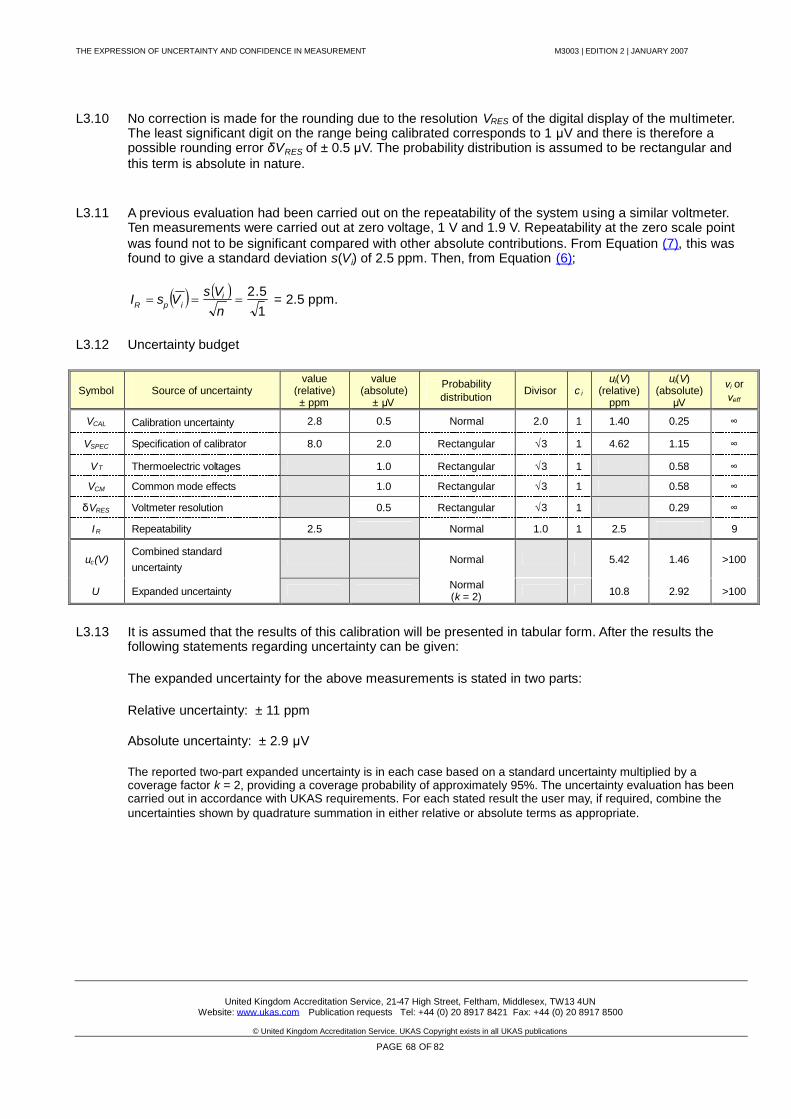
THE EXPRESSION OF UNCERTAINTY AND CONFIDENCE IN MEASUREMENT M3003 | EDITION 2 | JANUARY 2007
United Kingdom Accreditation Service, 21-47 High Street, Feltham, Middlesex, TW13 4UNWebsite: www.ukas.com Publication requests Tel: +44 (0) 20 8917 8421 Fax: +44 (0) 20 8917 8500
© United Kingdom Accreditation Service. UKAS Copyright exists in all UKAS publications
PAGE 68 OF 82
L3.10 No correction is made for the rounding due to the resolution VRES of the digital display of the multimeter.The least significant digit on the range being calibrated corresponds to 1 μV and there is therefore apossible rounding error δVRES of ± 0.5 μV. The probability distribution is assumed to be rectangular andthis term is absolute in nature.
L3.11 A previous evaluation had been carried out on the repeatability of the system using a similar voltmeter.Ten measurements were carried out at zero voltage, 1 V and 1.9 V. Repeatability at the zero scale pointwas found not to be significant compared with other absolute contributions. From Equation (7), this wasfound to give a standard deviation s(Vi) of 2.5 ppm. Then, from Equation (6);
15.2
nVsVsI i
ipR = 2.5 ppm.
L3.12 Uncertainty budget
Symbol Source of uncertaintyvalue
(relative)± ppm
value(absolute)
± μV
Probabilitydistribution
Divisor c i
ui(V)(relative)
ppm
ui(V)(absolute)
μV
νi orνeff
VCAL Calibration uncertainty 2.8 0.5 Normal 2.0 1 1.40 0.25 ∞
VSPEC Specification of calibrator 8.0 2.0 Rectangular √3 1 4.62 1.15 ∞
VT Thermoelectric voltages 1.0 Rectangular √3 1 0.58 ∞
VCM Common mode effects 1.0 Rectangular √3 1 0.58 ∞
δVRES Voltmeter resolution 0.5 Rectangular √3 1 0.29 ∞
IR Repeatability 2.5 Normal 1.0 1 2.5 9
uc(V)Combined standarduncertainty
Normal 5.42 1.46 >100
U Expanded uncertaintyNormal(k = 2) 10.8 2.92 >100
L3.13 It is assumed that the results of this calibration will be presented in tabular form. After the results thefollowing statements regarding uncertainty can be given:
The expanded uncertainty for the above measurements is stated in two parts:
Relative uncertainty: ± 11 ppm
Absolute uncertainty: ± 2.9 μV
The reported two-part expanded uncertainty is in each case based on a standard uncertainty multiplied by acoverage factor k = 2, providing a coverage probability of approximately 95%. The uncertainty evaluation has beencarried out in accordance with UKAS requirements. For each stated result the user may, if required, combine theuncertainties shown by quadrature summation in either relative or absolute terms as appropriate.
THE EXPRESSION OF UNCERTAINTY AND CONFIDENCE IN MEASUREMENT M3003 | EDITION 2 | JANUARY 2007
United Kingdom Accreditation Service, 21-47 High Street, Feltham, Middlesex, TW13 4UNWebsite: www.ukas.com Publication requests Tel: +44 (0) 20 8917 8421 Fax: +44 (0) 20 8917 8500
© United Kingdom Accreditation Service. UKAS Copyright exists in all UKAS publications
PAGE 69 OF 82
APPENDIX MASSESSMENT OF COMPLIANCE WITH SPECIFICATION
M1 Introduction
M1.1 In many situations it will be necessary to make a statement in calibration certificates or test reports aboutwhether or not the reported result complies with a given specification.
M1.2 For calibration activities, this will often be the case for general purpose test and measurementequipment. For measurement standards it is more likely that the measured value and expandeduncertainty will be of more interest to the user, and specification compliance is less relevant.
M1.3 For testing activities it is very likely that the result will have to be compared with specified limits in orderto arrive at a conclusion relating to conformance or fitness for purpose.
M2 Theory
M2.1 It has been shown elsewhere in this document that an uncertainty associated with a measurement resultwill usually take the form of a normal or Gaussian distribution centred around the reported value y of themeasurand Y.
M2.2 If the result y and the entirety of the distribution lie within the specified limits then it is clear thatcompliance with the specification has been demonstrated. Conversely, If the result y and the entirety ofthe distribution lie outside the specified limits then non-compliance with the specification has beendemonstrated.
M2.3 A “perfect” normal distribution has tails that extend to infinity in each direction, implying that there willalways be some doubt about whether or not compliance has or has not been demonstrated. In practice,an uncertainty budget is always based on a finite number of contributions, thereby limiting the amount bywhich the tails of the distribution extend away from the reported value.
M2.4 Nevertheless, it can be the case that one, or both, of the tails of the distribution significantly overlap one,or both, of the specification limits. This means that consideration has to be given to the area of thedistribution that is contained within the limits when assessing compliance with the specification.
M2.5 Furthermore, the implication of this is that compliance – or non-compliance – can only be stated inconjunction with an associated confidence level. This is because there will always be a possibility of one,or both, of the tails of the distribution overlapping the limits.
M2.6 This concept is illustrated in Figure 7 overleaf.
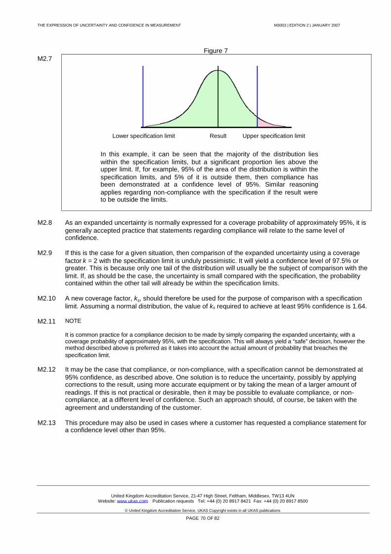
THE EXPRESSION OF UNCERTAINTY AND CONFIDENCE IN MEASUREMENT M3003 | EDITION 2 | JANUARY 2007
United Kingdom Accreditation Service, 21-47 High Street, Feltham, Middlesex, TW13 4UNWebsite: www.ukas.com Publication requests Tel: +44 (0) 20 8917 8421 Fax: +44 (0) 20 8917 8500
© United Kingdom Accreditation Service. UKAS Copyright exists in all UKAS publications
PAGE 70 OF 82
Figure 7M2.7
Lower specification limit Result Upper specification limit
In this example, it can be seen that the majority of the distribution lieswithin the specification limits, but a significant proportion lies above theupper limit. If, for example, 95% of the area of the distribution is within thespecification limits, and 5% of it is outside them, then compliance hasbeen demonstrated at a confidence level of 95%. Similar reasoningapplies regarding non-compliance with the specification if the result wereto be outside the limits.
M2.8 As an expanded uncertainty is normally expressed for a coverage probability of approximately 95%, it isgenerally accepted practice that statements regarding compliance will relate to the same level ofconfidence.
M2.9 If this is the case for a given situation, then comparison of the expanded uncertainty using a coveragefactor k = 2 with the specification limit is unduly pessimistic. It will yield a confidence level of 97.5% orgreater. This is because only one tail of the distribution will usually be the subject of comparison with thelimit. If, as should be the case, the uncertainty is small compared with the specification, the probabilitycontained within the other tail will already be within the specification limits.
M2.10 A new coverage factor, ks, should therefore be used for the purpose of comparison with a specificationlimit. Assuming a normal distribution, the value of ks required to achieve at least 95% confidence is 1.64.
M2.11 NOTE
It is common practice for a compliance decision to be made by simply comparing the expanded uncertainty, with acoverage probability of approximately 95%, with the specification. This will always yield a “safe” decision, however themethod described above is preferred as it takes into account the actual amount of probability that breaches thespecification limit.
M2.12 It may be the case that compliance, or non-compliance, with a specification cannot be demonstrated at95% confidence, as described above. One solution is to reduce the uncertainty, possibly by applyingcorrections to the result, using more accurate equipment or by taking the mean of a larger amount ofreadings. If this is not practical or desirable, then it may be possible to evaluate compliance, or non-compliance, at a different level of confidence. Such an approach should, of course, be taken with theagreement and understanding of the customer.
M2.13 This procedure may also be used in cases where a customer has requested a compliance statement fora confidence level other than 95%.
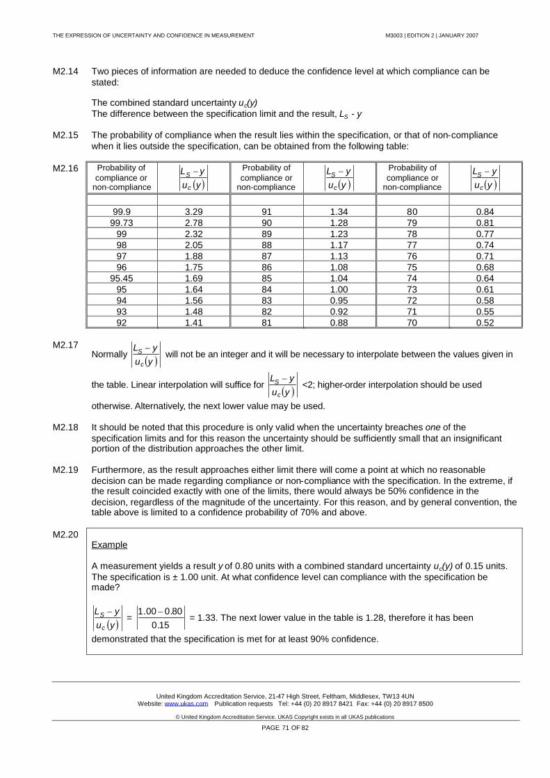
THE EXPRESSION OF UNCERTAINTY AND CONFIDENCE IN MEASUREMENT M3003 | EDITION 2 | JANUARY 2007
United Kingdom Accreditation Service, 21-47 High Street, Feltham, Middlesex, TW13 4UNWebsite: www.ukas.com Publication requests Tel: +44 (0) 20 8917 8421 Fax: +44 (0) 20 8917 8500
© United Kingdom Accreditation Service. UKAS Copyright exists in all UKAS publications
PAGE 71 OF 82
M2.14 Two pieces of information are needed to deduce the confidence level at which compliance can bestated:
The combined standard uncertainty uc(y)The difference between the specification limit and the result, LS - y
M2.15 The probability of compliance when the result lies within the specification, or that of non-compliancewhen it lies outside the specification, can be obtained from the following table:
M2.16 Probability ofcompliance or
non-compliance yuyL
c
S Probability ofcompliance or
non-compliance yuyL
c
S Probability ofcompliance or
non-compliance yuyL
c
S
99.9 3.29 91 1.34 80 0.8499.73 2.78 90 1.28 79 0.81
99 2.32 89 1.23 78 0.7798 2.05 88 1.17 77 0.7497 1.88 87 1.13 76 0.7196 1.75 86 1.08 75 0.68
95.45 1.69 85 1.04 74 0.6495 1.64 84 1.00 73 0.6194 1.56 83 0.95 72 0.5893 1.48 82 0.92 71 0.5592 1.41 81 0.88 70 0.52
M2.17Normally yu
yL
c
S will not be an integer and it will be necessary to interpolate between the values given in
the table. Linear interpolation will suffice for yuyL
c
S <2; higher-order interpolation should be used
otherwise. Alternatively, the next lower value may be used.
M2.18 It should be noted that this procedure is only valid when the uncertainty breaches one of thespecification limits and for this reason the uncertainty should be sufficiently small that an insignificantportion of the distribution approaches the other limit.
M2.19 Furthermore, as the result approaches either limit there will come a point at which no reasonabledecision can be made regarding compliance or non-compliance with the specification. In the extreme, ifthe result coincided exactly with one of the limits, there would always be 50% confidence in thedecision, regardless of the magnitude of the uncertainty. For this reason, and by general convention, thetable above is limited to a confidence probability of 70% and above.
M2.20Example
A measurement yields a result y of 0.80 units with a combined standard uncertainty uc(y) of 0.15 units.The specification is ± 1.00 unit. At what confidence level can compliance with the specification bemade?
yuyL
c
S =
15.080.000.1
= 1.33. The next lower value in the table is 1.28, therefore it has been
demonstrated that the specification is met for at least 90% confidence.
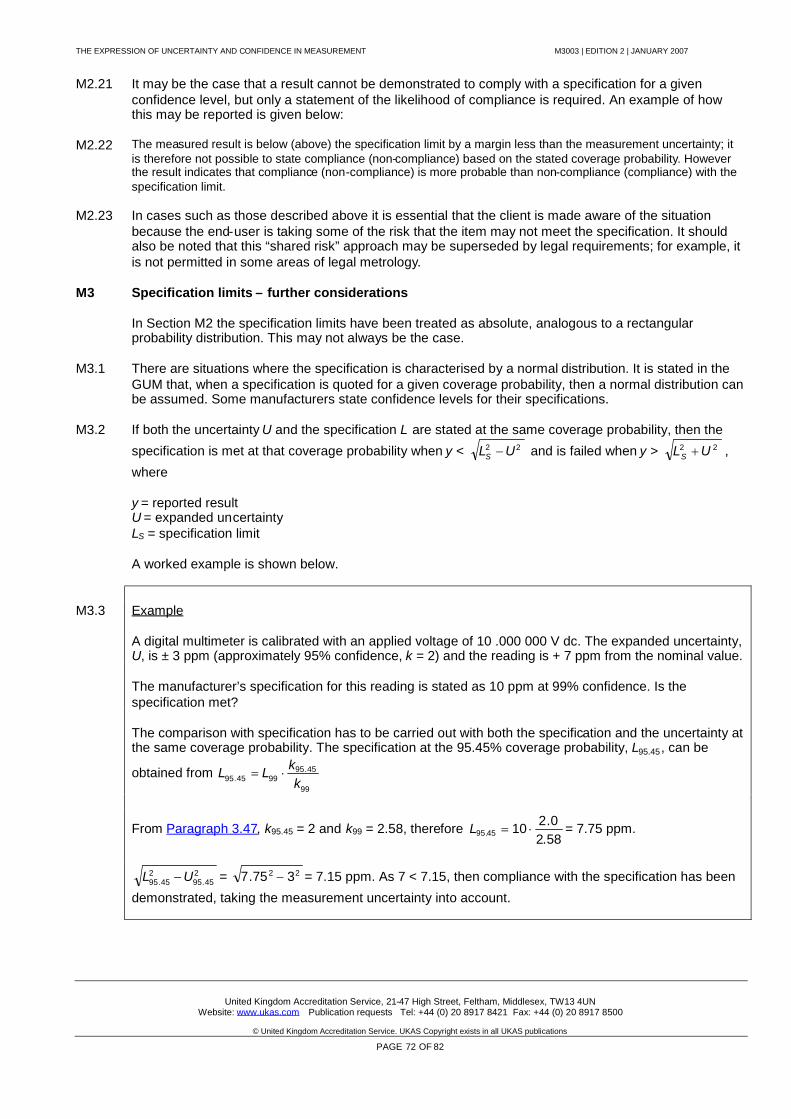
THE EXPRESSION OF UNCERTAINTY AND CONFIDENCE IN MEASUREMENT M3003 | EDITION 2 | JANUARY 2007
United Kingdom Accreditation Service, 21-47 High Street, Feltham, Middlesex, TW13 4UNWebsite: www.ukas.com Publication requests Tel: +44 (0) 20 8917 8421 Fax: +44 (0) 20 8917 8500
© United Kingdom Accreditation Service. UKAS Copyright exists in all UKAS publications
PAGE 72 OF 82
M2.21 It may be the case that a result cannot be demonstrated to comply with a specification for a givenconfidence level, but only a statement of the likelihood of compliance is required. An example of howthis may be reported is given below:
M2.22 The measured result is below (above) the specification limit by a margin less than the measurement uncertainty; itis therefore not possible to state compliance (non-compliance) based on the stated coverage probability. Howeverthe result indicates that compliance (non-compliance) is more probable than non-compliance (compliance) with thespecification limit.
M2.23 In cases such as those described above it is essential that the client is made aware of the situationbecause the end-user is taking some of the risk that the item may not meet the specification. It shouldalso be noted that this “shared risk” approach may be superseded by legal requirements; for example, itis not permitted in some areas of legal metrology.
M3 Specification limits – further considerations
In Section M2 the specification limits have been treated as absolute, analogous to a rectangularprobability distribution. This may not always be the case.
M3.1 There are situations where the specification is characterised by a normal distribution. It is stated in theGUM that, when a specification is quoted for a given coverage probability, then a normal distribution canbe assumed. Some manufacturers state confidence levels for their specifications.
M3.2 If both the uncertainty U and the specification L are stated at the same coverage probability, then the
specification is met at that coverage probability when y < 22 ULS and is failed when y > 22 ULS ,
where
y = reported resultU = expanded uncertaintyLS = specification limit
A worked example is shown below.
M3.3 Example
A digital multimeter is calibrated with an applied voltage of 10 .000 000 V dc. The expanded uncertainty,U, is ± 3 ppm (approximately 95% confidence, k = 2) and the reading is + 7 ppm from the nominal value.
The manufacturer’s specification for this reading is stated as 10 ppm at 99% confidence. Is thespecification met?
The comparison with specification has to be carried out with both the specification and the uncertainty atthe same coverage probability. The specification at the 95.45% coverage probability, L95.45, can be
obtained from99
45.959945.95 k
kLL
From Paragraph 3.47, k95.45 = 2 and k99 = 2.58, therefore58.20.21045.95 L = 7.75 ppm.
245.95
245.95 UL = 22 375.7 = 7.15 ppm. As 7 < 7.15, then compliance with the specification has been
demonstrated, taking the measurement uncertainty into account.

THE EXPRESSION OF UNCERTAINTY AND CONFIDENCE IN MEASUREMENT M3003 | EDITION 2 | JANUARY 2007
United Kingdom Accreditation Service, 21-47 High Street, Feltham, Middlesex, TW13 4UNWebsite: www.ukas.com Publication requests Tel: +44 (0) 20 8917 8421 Fax: +44 (0) 20 8917 8500
© United Kingdom Accreditation Service. UKAS Copyright exists in all UKAS publications
PAGE 73 OF 82
M4 Reporting compliance with specification
M4.1 If compliance or non-compliance with a specification is clearly demonstrated for a given confidence levelthen a statement to this effect can be made in calibration certificates and test reports. However caremust be taken to ensure that there is no implication that parameters that have not been measured alsocomply with a specification. For this reason a broad statement such as "the equipment complies with itsspecification" should not be made. A suggested statement of compliance is as follows:
The equipment complies with the stated specification at the measured points for the stated confidence level, dueallowance having been made for the uncertainty of the measurements.
This statement can be modified as necessary where non-compliance with a specification is to bereported.
M4.2 When making compliance or non-compliance statements, the specification and any relevant clauseswithin it should be unambiguously identified in the calibration certificate or test report.
M4.3 There may be cases where the uncertainty attainable for a given test or calibration is larger than thespecification for the item under consideration. Such situations should be subject to the contractarrangements between the laboratory and its customer. A statement regarding compliance should not begiven under these circumstances but a note should be included indicating those uncertainties associatedwith the measured values that are greater than the required specifications.
THE EXPRESSION OF UNCERTAINTY AND CONFIDENCE IN MEASUREMENT M3003 | EDITION 2 | JANUARY 2007
United Kingdom Accreditation Service, 21-47 High Street, Feltham, Middlesex, TW13 4UNWebsite: www.ukas.com Publication requests Tel: +44 (0) 20 8917 8421 Fax: +44 (0) 20 8917 8500
© United Kingdom Accreditation Service. UKAS Copyright exists in all UKAS publications
PAGE 74 OF 82
APPENDIX NUNCERTAINTIES FOR TEST RESULTS
N1 Introduction
N1.1 ISO/IEC 17025:2005 requires that “testing laboratories shall have and apply procedures for estimatinguncertainty of measurement”.
N1.2 It is recognised that the present state of development and application of uncertainties in testing activitiesis not as comprehensive as in the calibration fields, to which much of this document is addressed. It istherefore accepted that the implementation of ISO/IEC 17025:2005 criteria on this subject will take placeat an appropriate pace, which may differ from one field to another. However laboratories should be ableto satisfy requests from clients, or requirements of specifications, to provide statements of uncertainty.
N1.3 Testing laboratories should therefore have a defined policy covering the evaluation and reporting of theuncertainties associated with the tests performed. The laboratory should use documented proceduresfor the evaluation, treatment and reporting of the uncertainty.
N1.4 Some tests are qualitative in nature, i.e., they do not yield a numeric result. Therefore there can be nomeaning in reporting uncertainties directly associated with the test result. Nevertheless, there will beuncertainties associated with the underlying test conditions and these should be subject to the sametype of evaluation as is required for quantitative test results.
N1.5 The methodology for estimation of uncertainty in testing is no different from that in calibration andtherefore the procedures described in this document apply equally to testing results.
N2 Objectives
N2.1 The objective of a measurement is to determine the value of the measurand, ie the specific quantitysubject to measurement. When applied to testing, the general term measurand may cover manydifferent quantities, for example:
the electrical breakdown characteristics of an insulating material;
the strength of a material;
the concentration of an analyte;
the level of emissions of electromagnetic radiation from an appliance;
the quantity of micro-organisms in a food sample;
the susceptibility of an appliance to electric or magnetic fields;
the quantity of asbestos particles in a sample of air.
N2.2 A measurement begins with an appropriate specification of the measurand, the generic method ofmeasurement and the specific detailed measurement procedure. Knowledge of the influence quantitiesinvolved for a given procedure is important so that the sources of uncertainty can be identified.
THE EXPRESSION OF UNCERTAINTY AND CONFIDENCE IN MEASUREMENT M3003 | EDITION 2 | JANUARY 2007
United Kingdom Accreditation Service, 21-47 High Street, Feltham, Middlesex, TW13 4UNWebsite: www.ukas.com Publication requests Tel: +44 (0) 20 8917 8421 Fax: +44 (0) 20 8917 8500
© United Kingdom Accreditation Service. UKAS Copyright exists in all UKAS publications
PAGE 75 OF 82
N3 Sources of uncertainty
N3.1 There are many possible sources of uncertainty. As these will depend on the nature of the tests involved,it is not possible to give detailed guidance here. However the following general points will apply to manyareas of testing:
(a) Incomplete definition of the test - the requirement may not be clearly described, e.g. the temperature of atest may be given as 'room temperature'.
(b) Imperfect realisation of the test procedure; even when the test conditions are clearly defined it may notbe possible to produce the theoretical conditions in practice due to unavoidable imperfections in thematerials or systems used.
(c) Sampling - the sample may not be fully representative. In some disciplines, such as microbiologicaltesting, it can be very difficult to obtain a representative sample.
(d) Inadequate knowledge of the effects of environmental conditions on the measurement process, orimperfect measurement of environmental conditions.
(e) Personal bias and human factors; for example:
- Reading of scales on analogue indicating instruments.
- Judgement of colour.
- Reaction time, e.g. when using a stopwatch.
- Instrument resolution or discrimination threshold, or errors in graduation of a scale.
(f) Values assigned to measuring equipment and reference materials.
(g) Changes in the characteristics or performance of measuring equipment or reference materials since thelast calibration.
(h) Values of constants and other parameters used in data evaluation.
(i) Approximations and assumptions incorporated in the measurement method and procedure.
(j) Variations in repeated observations made under similar but not identical conditions - such randomeffects may be caused by, for example, electrical noise in measuring instruments, short-term fluctuationsin the local environment, e.g. temperature, humidity and air pressure, variability in the performance ofthe person carrying out the test and variability in the homogeneity of the sample itself.
N3.2 These sources are not necessarily independent and, in addition, unrecognised systematic effects mayexist that cannot be taken into account but contribute to error. This is one reason that participation ininter-laboratory comparisons, participation in proficiency testing schemes and internal cross-checking ofresults by different means are encouraged.
N3.3 Information on some of the sources of these errors can be obtained from:
(a) Data in calibration certificates - this enables corrections to be made and uncertainties to be assigned.
(b) Previous measurement data - for example, history graphs can be constructed and can yield usefulinformation about changes with time.
THE EXPRESSION OF UNCERTAINTY AND CONFIDENCE IN MEASUREMENT M3003 | EDITION 2 | JANUARY 2007
United Kingdom Accreditation Service, 21-47 High Street, Feltham, Middlesex, TW13 4UNWebsite: www.ukas.com Publication requests Tel: +44 (0) 20 8917 8421 Fax: +44 (0) 20 8917 8500
© United Kingdom Accreditation Service. UKAS Copyright exists in all UKAS publications
PAGE 76 OF 82
(c) Experience with or general knowledge about the behaviour and properties of similar materials andequipment.
(d) Accepted values of constants associated with materials and quantities.
(e) Manufacturers' specifications.
(f) All other relevant information.
These are all referred to as Type B evaluations because the values were not obtained by statisticalmeans. However the influence of random effects is often evaluated by the use of statistics; if this is thecase then the evaluation is designated Type A.
N3.4 Definitions are given in paragraph 3.10 for Type A evaluations and in paragraph 3.11 for Type Bevaluations. Further detail on the means of evaluation is given in Sections 4 and 5.
N3.5 It is recognised that in certain areas of testing it may be known that a significant contribution touncertainty exists but that the nature of the test precludes a rigorous evaluation of this contribution. Insuch cases, ISO/IEC 17025:2005 requires that a reasonable estimation be made and that the form ofthe reporting does not give an incorrect impression of the uncertainty.
N3.6 In some fields of testing it may be the case that the contribution of measuring instruments to the overalluncertainty can be demonstrated to be insignificant when compared with the repeatability of the process.Nevertheless, such instruments have to be shown to comply with the relevant specifications, normally bycalibration.
N3.7 Some analysis processes appear at first sight to be quite complex, for example there may be variousstages of weighing, dilutions and processing before results are obtained. However it will sometimes bethe case that the procedure requires standard reference materials to be subject to the same process, theresult being the difference between the readings for the analyte and the reference material. In suchcases, much of the process can be considered to be negatively correlated and the uncertainty ofmeasurement can be evaluated from the resolution and repeatability of the process; matrix effects mayalso have to be considered.
N4 Process
N4.1 The process of assigning a value of uncertainty to a measurement result is summarised below:
(a) Identify all sources of error that are likely to have a significant effect, and their relationship with themeasurand.
(b) Assign values to these using information such as described in N3.3, or in the case of Type A evaluations,calculate the standard deviation using Equations (5) and (6).
(c) Consider each uncertainty component and decide whether any are interrelated and whether a dominantcomponent exists (see D3 and Appendix C respectively).
(d) Add any interdependent components algebraically (i.e., account for whether they act together or canceleach other) and derive a net value.
(e) Express each uncertainty value as the equivalent of a standard deviation (see paragraph 3.24), takinginto account any sensitivity coefficients (see paragraphs 3.28 to 3.35).
(f) Take the independent components and the values of any derived net components and, in the absence ofa dominant component, combine them by taking the square root of the sum of the squares. This givesthe combined standard uncertainty (Equation (1)).
THE EXPRESSION OF UNCERTAINTY AND CONFIDENCE IN MEASUREMENT M3003 | EDITION 2 | JANUARY 2007
United Kingdom Accreditation Service, 21-47 High Street, Feltham, Middlesex, TW13 4UNWebsite: www.ukas.com Publication requests Tel: +44 (0) 20 8917 8421 Fax: +44 (0) 20 8917 8500
© United Kingdom Accreditation Service. UKAS Copyright exists in all UKAS publications
PAGE 77 OF 82
(g) Multiply the combined standard uncertainty by a coverage factor k, selected on the basis of the coverageprobability required, to provide the expanded uncertainty U (see paragraphs 3.42 to 3.44).
(h) Report the result and, if required, the expanded uncertainty, coverage factor and coverage probability inaccordance with Section 6.
N4.2 If one uncertainty contribution is significantly larger than the others then modifications may be requiredto this procedure. In the case of a dominant component derived from Type B evaluation, see AppendixC. If the non-repeatability of the system is significant, and its effects are evaluated by using a Type Aanalysis, it may be necessary to use the procedure in Appendix B.
N4.3 Further information regarding uncertainty evaluation for testing activities can be obtained from specialistpublications that address particular fields of testing, such as are described in References [7] and [8].

THE EXPRESSION OF UNCERTAINTY AND CONFIDENCE IN MEASUREMENT M3003 | EDITION 2 | JANUARY 2007
United Kingdom Accreditation Service, 21-47 High Street, Feltham, Middlesex, TW13 4UNWebsite: www.ukas.com Publication requests Tel: +44 (0) 20 8917 8421 Fax: +44 (0) 20 8917 8500
© United Kingdom Accreditation Service. UKAS Copyright exists in all UKAS publications
PAGE 78 OF 82
APPENDIX PELECTRONIC DATA PROCESSING
P1 Introduction
P1.1 Due to the nature and quantity of the calculations involved it is inevitable that some form of electronicprocessing will be involved in these calculations. This Appendix gives brief details of precautions thatmay be necessary under these circumstances. Mention is also made of other techniques of uncertaintyevaluation that electronic data processing has made practical.
P2 Use of calculators
P2.1 Most scientific calculators are easily capable of all the calculations required for the evaluation ofmeasurement uncertainty. It is recommended that readers of this document gain familiarity with thefunctions involved by practicing the calculations presented in Appendix K - this can give rise to a betterunderstanding of the process as well as giving the users confidence in their own abilities.
P2.2 It is also recommended that, where possible, intermediate results are stored in the calculator memory foruse later, or are written down to a reasonable amount of significant figures, in order to prevent thecumulative effects of rounding errors having a significant effect on the result. Most scientific calculatorswork with sufficient accuracy so that they do not in themselves introduce any significant errors - with onenotable exception (see Section P4).
P3 Use of spreadsheets
P3.1 The widespread use of personal computers has made repetitive calculations a much easier process thanin the past. It is possible to construct a spreadsheet using the various equations presented in thisdocument in order to perform the uncertainty calculations. The time spent constructing the spreadsheetcan easily be recovered by the subsequent ease of producing, and amending, uncertainty budgets.
P3.2 It is recommended that a sample of results produced by a spreadsheet programme is checked manuallyusing a scientific calculator to ensure that correct results are being generated.
P4 Calculation of standard deviations
P4.1 Many scientific calculators include statistical functions for calculation of standard deviations inaccordance with Equation 5. The calculator key associated with this function will usually be marked σn-1
or, sometimes, s.
P4.2 It will often be the case that this particular function is not capable of evaluating small values of standarddeviation correctly. The following data set is presented as an example:
1000.025 1000.015 1000.019 1000.021
P4.3 The value of s that is obtained from this data, using Equation 5, should be 0.004163. Most calculatorswill either:
(a) Display an error message, or
(b) Display a value of zero, or
(c) Display an incorrect non-zero value.

THE EXPRESSION OF UNCERTAINTY AND CONFIDENCE IN MEASUREMENT M3003 | EDITION 2 | JANUARY 2007
United Kingdom Accreditation Service, 21-47 High Street, Feltham, Middlesex, TW13 4UNWebsite: www.ukas.com Publication requests Tel: +44 (0) 20 8917 8421 Fax: +44 (0) 20 8917 8500
© United Kingdom Accreditation Service. UKAS Copyright exists in all UKAS publications
PAGE 79 OF 82
P4.4 A solution to this problem is to use only the few least significant digits in the set of data. So, for the dataabove, the numbers 0.025, 0.015, 0.019 and 0.021 can be entered, yielding the correct value of s(qj):0.00416.
NOTE
This could equally have been evaluated using just the last two digits, i.e. 25, 15, 19 and 21. However it is useful toinclude a decimal point, as this will then appear in the correct place in the results thereby minimising the likelihoodof errors being made.
P4.5 It is possible that electronic spreadsheets will also suffer from similar errors therefore suitable checksshould be devised to evaluate any such effects.
P5 Other techniques
P5.1 The use of high speed data processing has opened new avenues for the analysis of uncertainty. Onesuch technique is known as Monte Carlo simulation.
P5.2 In a Monte Carlo simulation the mathematical model of the underlying system is run over and overagain, each time using a different set of random numbers representing the input variables. Each of thesesets of random numbers combines via the model to represent a different outcome. Each run of themodel is called a simulation, or trial, and at the end of each trial the outcome of the process is recorded.Each different outcome arises, through the measurement model, corresponding to a particular set ofrandom numbers being applied to it. If the model is a good representation of the real-world system, then,by running a large enough number of trials (each with a different set of random numbers), the wholerange of possible outputs can be produced; these form the distribution of the output.
P5.3 Sampling techniques, such as Monte Carlo simulation, provide an alternative approach to uncertaintyevaluation in which the propagation of uncertainties is undertaken numerically rather than analytically.Such techniques are useful for validating the results returned by the application of the GUM, as well asin circumstances where the assumptions made by the GUM do not apply. In fact, these techniques areable to provide much richer information, by propagating the distributions (rather than just theuncertainties) of the inputs x i through the measurement model f to provide the distribution of the outputy. From the output distribution confidence intervals can be produced, as can other statistical information.
P5.4 Another method of uncertainty analysis is by the use of Bayesian statistics; this is based on the conceptof degree of belief. Bayes’ Theorem gives the ’posterior’ odds on the correctness of a belief (given thenew evidence that has just been observed), making use of the ’prior’ odds that the belief is correct, i.e.an estimate of the plausibility of the belief before one has the new data. A concept of likelihood ratioallows the ‘prior’ odds to be adjusted according to the each piece of new evidence. Another iteration isthen performed using the next piece of evidence, and so on until all the evidence is used and aprobability associated with the belief is obtained.
P5.5 Bayes’ Theorem is particularly useful for analysis of qualitative data, where the conventional GUMmethodology is not appropriate. It can also be applied to the expression of professional opinions thatmay appear in test reports.
THE EXPRESSION OF UNCERTAINTY AND CONFIDENCE IN MEASUREMENT M3003 | EDITION 2 | JANUARY 2007
United Kingdom Accreditation Service, 21-47 High Street, Feltham, Middlesex, TW13 4UNWebsite: www.ukas.com Publication requests Tel: +44 (0) 20 8917 8421 Fax: +44 (0) 20 8917 8500
© United Kingdom Accreditation Service. UKAS Copyright exists in all UKAS publications
PAGE 80 OF 82
APPENDIX QSYMBOLS
The symbols used are taken mainly from the GUM. The meanings have also been described further in the text,usually where they first occur, but are summarised here for convenience of reference.
a i Estimated semi-range of uncorrelated systematic component of uncertainty, probabil ity distributionsunknown, where i = 1 ..... N.
ad A systematic component of uncertainty that so dominates other contributions to uncertainty inmagnitude that special consideration has to be given to its presence in calculating the expandeduncertainty.
ci Sensitivity coefficient used to multiply the value x i of an input quantity Xi to express it in terms of themeasurand Y.
f Functional relationship between the measurand Y and the input quantities Xi on which Y depends,and between output estimate y and input estimates xi upon which y depends.
∂f/∂x i Partial derivative with respect to input quantity Xi of the functional relationship f between themeasurand and the input quantities.
k Coverage factor (general).
kp Coverage factor used to calculate an expanded uncertainty Up for a specified coverage probabilityp.
ks Coverage factor chosen for the purpose of comparison with a specification limit.
m Number of readings or observations that are used for the evaluation of s(q j), if different from n.
n Number of readings or observations that contribute to a mean value.
N Number of input estimates xi on which the value of the measurand depends.
q j jth repeated observation of randomly varying quantity q.See Note 1 below.
q Arithmetic mean or average of n repeated observations of randomly varying quantity q.
p Coverage probability or level of confidence expressed in percentage terms or in the range zero toone.
σ The standard deviation of a population of data using all the samples in that population.
s(qj) Estimate of the standard deviation σof the population of values of a random variable q based on alimited sample of results from that population.See Note 1 overleaf.
qs Experimental standard deviation of the mean value q .
tp(νeff) Student t-factor for νeff degrees of freedom corresponding to a given coverage probability p.

THE EXPRESSION OF UNCERTAINTY AND CONFIDENCE IN MEASUREMENT M3003 | EDITION 2 | JANUARY 2007
United Kingdom Accreditation Service, 21-47 High Street, Feltham, Middlesex, TW13 4UNWebsite: www.ukas.com Publication requests Tel: +44 (0) 20 8917 8421 Fax: +44 (0) 20 8917 8500
© United Kingdom Accreditation Service. UKAS Copyright exists in all UKAS publications
PAGE 81 OF 82
u(xi) Standard uncertainty of input estimate xi .
uc(y) Combined standard uncertainty of output estimate y.
U Expanded uncertainty of output estimate y that describes the measurand as an interval Y = y ± U,with a high coverage probability.
Up Expanded uncertainty of output estimate y that describes the measurand as an interval Y = y ± Up,with a specified coverage probability p.
ν Degrees of freedom; in general, the number of terms in a sum minus the number of constraints onthe terms of the sum.
νi Degrees of freedom of standard uncertainty u(xi) of input estimate xi.
νeff Effective degrees of freedom of uc(y) used to obtain tp(νeff)
NOTE 1 The GUM uses the symbols qk and s(qk) where qj and s(qj) are used here. M3003 uses the subscript j instead of k in order toavoid any possible confusion with the coverage factor k.
THE EXPRESSION OF UNCERTAINTY AND CONFIDENCE IN MEASUREMENT M3003 | EDITION 2 | JANUARY 2007
United Kingdom Accreditation Service, 21-47 High Street, Feltham, Middlesex, TW13 4UNWebsite: www.ukas.com Publication requests Tel: +44 (0) 20 8917 8421 Fax: +44 (0) 20 8917 8500
© United Kingdom Accreditation Service. UKAS Copyright exists in all UKAS publications
PAGE 82 OF 82
APPENDIX RREFERENCES
1 BIPM, IEC, IFCC, ISO, IUPAC, IUPAP, OIML. Guide to the Expression of Uncertainty inMeasurement. International Organisation for Standardization, Geneva, Switzerland. ISBN 92-67-10188-9, First Edition 1993.
BSI Equivalent:
BSI PD 6461: 1995, Vocabulary of metrology, Part 3. Guide to the Expression of Uncertainty inMeasurement. BSI ISBN 0 580 23482 7
2 European cooperation for Accreditation, EA-4/02 Expression of the Uncertainty of Measurement inCalibration, December 1999
3 HARRIS, I.A and WARNER, F.L. Re-examination of mismatch uncertainty when measuringmicrowave power and attenuation. IEE Proceedings, Vol 128 Pt H No 1, February 1981.
4 DIETRICH, C.F. Uncertainty, Calibration and Probability: The Statistics of Scientific and IndustrialMeasurement Uncertainty, Institute of Physics, January 1991.
5 National Physical Laboratory, ANAMET Connector Guide, Edition 2.
6 United Kingdom Accreditation Service, Calibration of Weighing Machines, LAB14 Edition 4,November 2006.
7 United Kingdom Accreditation Service, The Expression of Uncertainty in EMC Testing, LAB34Edition1, August 2002.
8 EURACHEM/CITAC Guide: Quantifying Uncertainty in Analytical Measurement, QUAM:2000.1,Second Edition, 2000. ISBN 0 948926 15 5