The Expansion of Consumption and the Dynamics of

Welfare of the Brazilian Families: An Analysis of the

Decomposition of Poverty and Inequality

Leonardo S. Oliveira (Institute of Geography and Statistics, Brazil), Viviane C.C. Quintaes

(Institute of Geography and Statistics, Brazil), Luciana A. Dos Santos (Institute of Geography

and Statistics, Brazil), and Debora F. De Souza (Institute of Geography and Statistics, Brazil)

Paper prepared for the 34

th IARIW General Conference

Dresden, Germany, August 21-27, 2016

7D: Well-Being III

Time: Friday, August 26, 2016 [Morning]

The expansion of consumption and the welfare dynamics of the Brazilian

families: a decomposition analysis of poverty and inequality

BY LEONARDO S. OLIVEIRA* VIVIANE C.C. QUINTAES* LUCIANA A. DOS SANTOS*

DEBORA F. DE SOUZA*

Abstract

This article gathers analyses that involve dynamic aspects of welfare, inequality and poverty in Brazil in the

periods of 2002-2003 and 2008-2009 from the perspective of the per capita consumption. By means of the

data of the Brazilian Family Expenditure Survey (POF), from the construction of the consumption aggregates,

the evolution of the consumption structures in the period mentioned above are evaluated, according to the

location of families in the Major Brazilian Regions and in the urban and rural areas. For this purpose, the

study incorporates the value of services related to existing durable goods in the households in each edition

of the survey. The study resorts to graphical and dominance analyses as well as to the calculation of functions

that allow measuring and separating the effects of growth and redistribution over social welfare. The role of

the consumption structure in changes made to the levels of welfare and poverty is evaluated according to

static and dynamic decompositions. The main results indicate that the Durable goods strongly contributed

for the growth of consumption and social welfare but they were also a limiting factor for the inequality

reduction. In relation to poverty, we observed that in all the geographic areas that were studied poverty in

2008-2009 was lower than in 2002-2003 for the different measures and poverty lines that were used in this

study.

Keywords: Gini Index, Living standards, General Welfare, Consumer price index, Shapley Value

JEL: C02, C43, D31, D69, I31

Brazilian Institute of Geography and Statistics (IBGE)

leonardo.s.oliveira@ibge.gov.br; viviane.quintaes@ibge.gov.br;

luciana.santos@ibge.gov.br; debora.souza@ibge.gov.br

IBGE is exempt from any responsibility related to the opinions, information, data and concepts stated in this article that are of

exclusive responsibility of the authors.

The authors would like to thank Paulo Roberto Coutinho Pinto, Juliano Junqueira and André Martins for his collaboration and Marta

Antunes, Nícia Brendolin and Isabel Martins for their comments.

2

1. Introduction

The complexity and multidimensionality of poverty and inequality make the definition of an

appropriate indicator, which captures the welfare of people and families, one of the essential

issues for studying and dimensioning these themes. The purpose of this work is to contribute

with the analyses of these topics by constructing an aggregate of family consumption based on

data of the Brazilian Family Expenditure Survey (Pesquisa de Orçamentos Familiares - POF)

carried out in 2002-2003 and 2008-2009, following the literature and recent advances, in order

to allow measuring and analyzing the welfare, the poverty, the inequality of families with

emphasis on their dynamic aspects.

Oliveira et al (2016), as recommended by Hentschel and Lanjow (1996), Slesnick (2001), Lanjow

and Lanjow (2001), Deaton and Zaidi (2002), ILO-ICLS-17 (2003), Haughton and Khandker (2009),

Lanjow (2009), Stiglitz, Sen and Fitoussi (2009) and OCDE (2013), constructed a consumption

aggregate based on the POF 2008-2009, selected non sporadic expenses, which in general

represent welfare gains, calculate the value of services related to durable goods by the use cost,

the value of food costs when necessary and applied spatial deflators. As a result, they checked

which of the suggested consumption aggregates reflects the choices of the families in multiple

dimensions and allows the analysis of the socioeconomic welfare from POF data.

POF1 is a household survey conducted by IBGE that provides information about the consumption

pattern of the Brazilian families. By standardizing the calculation of the consumption aggregate

in the two editions of the survey (POF 2002-2003 and POF 2008-2009), we enabled the

monitoring of the evolution of welfare among the Brazilian families during a period of high

economic growth and expansion of consumption. The POF editions carried out in 2002-2003 and

2008-2009, since they are the only ones that include all the national territory, enable the

comparison at the geographic level and of the consumption structure from the expense items.

In this work, we followed the construction of the consumption aggregate for the period of 2008-

2009 adopted in Oliveira et al (2016), we was also applied to data of the POF edition carried out

in 2002-2003 enabling an analysis of consumption evolution, welfare, inequality and poverty

between 2002-2003 and 2008-2009. As emphasized in Ferreira (2010), a great deal of attention

has been given to dynamic aspects of welfare, which show how the distinct growth rates of

consumption (or income) of the poorer and the richer determine the values of inequality,

poverty and the mean consumption (or income) over time. The author suggested that studying

this triangular relationship growth-poverty-inequality only under the macroeconomic

perspective limits the analyses, considering the three vertexes of the triangle are moved by the

dynamic interaction of individual incomes at the microeconomic level. The same argument can

be used for consumption.

The period analyzed in this work was marked by important aspects of the internal and external

economic scenarios that worth mentioning. In Brazil, the years between 2002 and 2009 were

1The first edition of the POF was in 1987-1988 and the main purpose was to update the consumption matrix for the calculation of

product considerations related to the index of national price and National Bills. Thus, a limited set of products was searched only for the metropolitan regions of the country, and the same happened with the second edition carried out in 1995-1996. Only in the POF

edition carried out in 2002-2003 the purpose of the survey was expanded and the geographic coverage started considering all the

national territory.

3

marked by a sharp economic growth, with real increase around 25% in the GDP, tax incentive

for production and acquisition of durable goods, such as electronics and vehicles, declining

interest rates (44%) and expansion of credit supply2. This period was called “consumption boom”

in the country. In the international context, it is worth mentioning that at the outbreak of the

subprime crisis, in 2008, initiated in the United States but with global effects, the POF had just

started and the effects of the crisis may have been captured by the survey.

The impact of this economic growth on the reduction of poverty and inequality in this period

has already been analyzed in several works, especially under an income perspective. The main

source of these studies was the National Household Sample Survey (Pesquisa Nacional por

Amostra de Domicílios - PNAD), sample household survey of annual frequency conducted by

IBGE3. Barros et al (2007) showed a decrease in the Brazilian inequality that took place between

2001 and 2005. The authors investigated non-labor incomes to find out which one played a more

relevant role on the decrease of inequality. The public transfers, in special, the retirements and

the pensions caused the greater impact, while the effect of cash transfers social programs,

Benefício de Prestação Continuada (BPC) and Bolsa Família, on the reduction of inequality was

practically all a reflection of coverage expansion of such programs.

Neri (2011), on the other hand, analyzed the transition of the poorest social classes to the middle

class, the so-called class C, between 2001 and 2009. During this period, the per capita income of

the 10% poorer population in Brazil rose 69%, while the 10% richer rose only 13%. Between 2003

and 2009, the classes “AB” and “C” increased their population to 6.6 million and 29 million,

respectively. In contrast, there was a reduction in the number of people who belong to the

poorer classes “D”, 2.5 milllion, and “E”, 20.5 milllion. Also, there was a decrease in the

inequality of income considering the evolution of the Gini index in the same period from 0.58 in

2003 to 0.55 in 2009. IPEA (2012) conducted another study that analyzed this Brazilian

socioeconomic period, which highlighted that the downward trend of poverty during the first

decade of the year 2000 was not interrupted by the financial crisis in 2008. The population

whose household income per capita is below the poverty line dropped 11.4 p.p. between 2003

and 2008, while from 2008 until 2009 the reduction was of only 0.6 p.p.

Hoffmann (2010) also studied the evolution of the distribution of the Brazilian household income

per capita, but he used the POFs carried out in 2002-2003 and 2008-2009. Since the capture of

income in the POF is more detailed than in the PNAD, by including information related to the

production value to self-consumption and asset variation, the author investigates if the

reduction in inequality as observed by PNAD is also obtained by POF for this period. He found a

decrease in inequality measured by the Gini index from 0.59 in 2002-2003 to 0.56 in 2008-2009.

Despite the contribution of these studies over the evolution of income and welfare of the

Brazilian population during this period, only a few works evaluated the evolution under the

consumption perspective itself, or even the expense perspective4. One example of these studies

is Campolina and Gaiger (2013) who elaborated a study based on the evolution of expenditure.

2Basic prices in the Gross Domestic Product (GDP): reference 2010 – IPEADATA: http://www.ipeadata.gov.br;

Interest rate - SELIC (Special System of Settlement and Custody). Brazilian Central Bank http://www.bcb.gov.br/Pec/Copom/Port/taxaSelic.asp. 3See also Barros et al (2006a;2006b); Ferreira et al (2006); Soares (2006). 4See Gaiger Silveira et al (2007).

4

The authors used the history of the POFs carried out in the periods from 1987-1988 until 2008-

2009 to study the changes in the Brazilian consumer market starting from the hypothesis of

homogenization of demand profiles and expansion of credit. Considering a descriptive analysis,

they evaluated the behavior of the participation of expense groups in the survey according to

the social classes in all the Brazilian territory (2003-2009) and according to the metropolitan

areas in the period from 1988 until 2009 since they have the same geographic coverage. They

showed the increase in participation between 2003 and 2009 of the 70% poorer over the total

value of the household monetary budget was of 0.4p.p., accounting for 31.2%, while the 10%

richer maintained their participation. In spite of the increase of 2p.p. in the participation of half

the poorer population in health, education and personal services expenses, it was with expenses

related to the acquisition of electronics that the 70% poorer population had a significant

increase in participation (38% in 2003 versus 42% in 2009).

This work proposes the evaluation of how the impact of the growth in consumption and its

structure reflect upon the welfare, the poverty and the decrease in inequality among the

Brazilian families, especially under the dynamic aspect. By including the period 2002-2003 in the

analyses, this works expands what was done by Oliveira et al (2016) that analyzed the effects of

welfare, inequality, poverty and vulnerability of families from the consumption aggregate only

for the period of 2008-2009. Considering the consumption aggregates that were constructed,

we notice the growth of consumption along the distribution, calculate the usual inequality and

welfare as well as use analytical5 (Rao, 1969; Shorrocks, 1982; Jenkins, 1995) and counterfactual

(Shorrocks, 2012) decompositions for a dynamic analysis of consumption and its components.

These components were defined as: i) Food; ii) Durable goods; iii) Housing; iv) Education, health,

and transportation; and v) Other goods.

In addition to this introduction, this work has another five sections. The first one deals with the

construction of consumption aggregates from information obtained from the POFs in the

periods 2002-2003 and 2008-2009. Next, we make a descriptive analysis of the mean

consumption per capita behavior and its components, according to Brazil, Major Regions and

Urban and Rural Areas. In section three, we evaluate the effect of the consumption variation

over the welfare and the inequality by static and dynamic decompositions. Similarly, in section

four, we present static and dynamic counterfactual decompositions that show the impact of the

consumption behavior and its components over poverty. Finally, in the last section, we make

the final comments with some conclusions about the results that were presented and

suggestions of improvements and further development in this study.

2. Consumption Aggregate

The construction of the consumption aggregate is the first and essential step of this work, since

it is a complex exercise that requires a detailed and precise breakdown of the expenses that

should be included or not with the purpose of comparing the levels of welfare and the correct

ordination/hierarchy of different families. This breakdown is oriented by the applied literature

and the theoretical hypothesis about the contribution of different goods and services to welfare,

as well as the necessary adaptations to Brazilian culture and habits.

5See Lerman and Yitzhaki (1985); Soares (2006); Hoffmann (2006) for analytical decompositions and Shapley (1953);

Barros et al (2006); Duclos and Araar (2006); Azevedo et al (2013) for counterfactual decompositions.

5

The Brazilian Family Expenditure Survey (Pesquisa de Orçamentos Familiares - POF) used as

source of information is a sample survey conducted by IBGE, collected during twelve months,

which investigates the topics expenses, income and asset variation of families, basic aspects for

the analysis of household income, and some factors related to the subjective evaluation of the

living conditions. The POF is organized in seven questionnaires that are subdivided in frames,

where each one of them refers to a type of expense, income or survey topic. The survey editions

of 2002-2003 and 2008-2009 created a database with information related to 3.860 and 4.728

records of distinct items, respectively, (products, goods, services, etc), which had to be

identified, reconciled and classified one by one for the construction of the consumption

aggregates.

The construction of the consumption aggregates used here followed the same methodology

used in Oliveira et al (2016) that, by using the recommendations of Hentschel and Lanjow (1996),

Slesnick (2001), Lanjow and Lanjow (2001), Deaton and Zaidi (2002), ILO-ICLS-17 (2003),

Haughton and Khandker (2009), Lanjow (2009), Stiglitz, Sen and Fitoussi (2009) and OCDE

(2013), selected expense items that enabled the comparison between the welfare levels of

families, classifying them in five groups: i) Food; ii) Durable goods; iii) Housing; iv) Education,

health and transportation; and v) Other goods. In order to define which expense items should

compose the consumption aggregate, the following criteria were adopted: i) The expense item

should not be of sporadic acquisition; ii) The acquisition should be for the consumption unity

itself6, that is, the acquisition of the good will increase the welfare of the consumption unit under

analysis and not that of another unit; iii) The item contributed for the comparison of welfare

among different families and their correct ordination. Besides, it was necessary to treat the

following information: imputation of the value of the food that is consumed for the families that

did not have these expenses in the reference period and; the calculation of the service value for

the use cost of household durable goods (that differs from the acquisition cost). The last step of

the construction of consumption aggregates consisted of correcting the values obtained by the

use of price deflators.

In order to construct the two consumption aggregates, in such a way that it is possible to

compare them, some small adjustments had to be made regarding the consumption aggregate

that was created in Oliveira et al (2016), especially in what concerns the spatial deflators. Next,

we will briefly explain the steps of the treatment given to items of each expense group analyzed

in the consumption aggregates in both periods.

2.1. Food Expenditure

All the food expenditure was included in the aggregate. However, there was a need to treat this

information considering that 3.8%, in 2003, and 5.8%, in 2008, of the consumption units that

were interviewed in the survey did not have food expenditure. This behavior does not cause

surprise, because the POF uses a short reference period (7 days) to capture the acquisition of

6Consumption Unit: in the Brazilian Family Expenditure Survey, the concept of Consumption Unit comprises a single resident or group of residents who share the source of food, which can be approximated to the idea of household units or family. For further details, see IBGE (2008).

6

food. Thus, since it is a very short interval, it is common that some families did not have food

expenditure, and it does not mean they did not consume this type of goods during the period of

seven days.

Therefore, considering this null food expenditure can change the levels of social welfare,

inequality and poverty of families, an imputation was made in the null food expenditure by using

the Propensity Score Method (Rosenbaum e Rubin, 1983). This method compares the estimated

probabilities of the units to present zero food expenditure in two groups called control and

treatment. The treatment group was composed of units that did not declare food consumption

and the control group was composed of the units with food consumption different from zero.

For each unit of the treatment group, we search the control group for a donor unit of food

consumption. The probability of the donor should be as close as possible of the probability

estimated for the unit of the treatment group. In appendix 1, we present the variables that

explain the logit model that was applied and the density function of the per capita consumption

with and without food expenditure imputed for the POF editions carried out in 2002-2003 and

in 2008-2009.

2.2. Durable Goods

The inclusion of durable goods in the consumption aggregate was one of the main contributions

made in Oliveira et al (2016). According to the authors, the possession of durable goods is an

important indicator of welfare of the consumption units, but there is a difficulty in using it

because most acquisition prices of these goods are elevated and they can impact the comparison

among families that already have such goods and the remaining ones that were acquiring them

only in the reference period of the survey. By considering only the calculated service value by

the use cost of each durable good and not the acquisition value, this problem was solved. For

further details, see Oliveira et al (2016).

As in Oliveira et al (2016), only the items of durable goods that are part of the “Inventory of

durable goods of the main residence” (frame 14) were included in the consumption aggregates.

This selection is necessary because, to calculate the value of services by the use cost, we need

information of the acquisition date of goods and they are only captured in frame 14 of the POF.

The list of inventory goods is related to technology and the frequency of acquisition according

to the period of each survey, and there are some small differences between the POF inventory

of 2002-2003 and the POF inventory of 2008-2009. Since technology is in intense evolution,

mainly in what concerns electronics, many goods of high frequency of acquisition in a survey fell

into disuse in the following survey or were no longer indications of welfare, such as VCR, floor

polisher, recorder, cassette player and laser read-head of disc player. On the other hand, other

goods that were not yet created or that were not commonly acquired became popular during

the period between the surveys and were included in the inventory of the consumption units

such as, for example, the electric oven and the food processor. In appendix 2, we list the two

inventories of the corresponding surveys so as to show the items used in the composition of

durable goods.

7

2.3. Housing

In the housing group, we included the following expense types: rent, utility services, home

refurbishment, furniture and household articles, electronics and electronic fixing and cleaning

material.

2.4. Education, health and transportation

Despite the distinct nature, education, health and transportation expenses were grouped

because they deserve differentiated treatment and evaluation. Some items of these

components can be interpreted as “regrettable needs”7 and reveal little about the

choices/preferences of consumers or even about their rank/hierarchy of family welfare.

According to Oliveira et al (2016), based on Lanjow (2009) and Deaton and Zaidi (2002), the

health and education expenses could be included in the aggregate if their elasticity8 related to

the total expenses was greater than one. Thus, the total education expenses and the health

expenses related to healthcare and dental insurance contracts were included (POF´s block 42).

The elasticity values found for education and health were, respectively, 1.42 and 0.87 in 2002-

2003 and 1.28 and 0.92 in 2008-2009.

Now, regarding the transportation expenditures, we decided to exclude the expenses with mass

transportation (bus, subway, train, ferryboat, alternative means of transportation and their

connections), since the high values are associated with a longer distance between the residence

and the workplace, and these areas are usually peripheral, as suggested in Nordhaus and Tobin

(1972) and Sen, Stiglitz and Fitoussi, (2009). The other expenses related to private

transportation, such as own car (fuel, parking, toll and car wash), taxi, plane and car rental were

included because, to a certain extent, these expenses reflect choices and individual preferences.

The travel expenses of POF´s block 41 had a distinct treatment when compared with the one

adopted by Oliveira et (2016), because the POF edition carried out in 2002-2003 does not inform

the reason of the trip. As a result, it is not possible to distinguish the leisure trip from the other

ones. In order to compare both surveys, we included all the information related to travel

expenses registered in POF´s block 41 in the editions carried out in 2002-2003 and 2008-2009.

2.5. Other goods

This group aggregates expenses related to clothing, culture and leisure, personal services

(manicure, pedicure, barber, hairdresser etc.), hygiene and personal care, smoking habits and

other miscellaneous expenditures. Among the miscellaneous expenditures, were considered

7 A "regrettable necessity" involves acquisitions under differentiated circumstances, which make it more difficult to measure the

welfare based on consumption/expense: (1) It can involve undesirable conditions (in many cases of short term) that negatively

impact the welfare of families/individuals and lead to an increase in expenses only to mitigate such impacts; (2) It can also involve

expenses that, for some people, have a purely instrumental nature, making them difficult to avoid and necessary only as a means to acquire a "second item or objective". Including the expenses in these items, without a proper treatment of the loss of welfare

involved, would lead to an inappropriate measurement of the “long term” welfare, indicating, for example, that a person who spent a

lot of money on medication when he/she was sick is better than someone who did not have this expense. Oliveira et al (2016), Lanjow (2009) and Deaton and Zaidi (2002) suggested the exclusion of many of these items. 8The concept of elasticity associates the percentage change in y with a given variation in x. It is possible estimate the elasticity of

expenses with a specific item related to the total expense by the following model: ln ln ,i i iy x where yi is the expense

with the item in question, xi is the total expense for a given observation i. The coefficient β measures the elasticity of y in relation to

x. Lanjow and Lanjow (2001) suggested a similar approach to avoid the impact of measurement mistakes on the behavior of the consumption aggregate and the remaining results, especially the measurement of poverty.

8

expenses with other properties, parties, communications and professional services, such as

registry, lawyer and brokers.

The expenses with wedding, wedding dress and funeral and the rare and expensive acquisitions

were not included in the aggregate, according to orientation provided by Deaton and Zaidi

(2002) and Haughton and Khandker (2009), Lanjow (2009).

Frequent expenses with public services (such as light, water, sewage, condominium, parking,

etc) related to other properties of the consumption unit and used for self benefit (beach house,

for example) were included, while expenses with taxes, social contributions, pensions, subsidies,

donations to other families and private pension were excluded. Banking expenses were included

in the consumption aggregate, except for banking services with interests of overdraft and credit

card.

2.6. Price Deflator

In order to compare the consumption pattern among different geographic contexts, it is

necessary to apply a spatial deflator, which corrects differences between prices. According to

Oliveira et al (2016), the deflators were created for the following twenty geographic contexts:

Metropolitan Regions (Belém, Fortaleza, Recife, Salvador, Belo Horizonte, Rio de Janeiro, São

Paulo, Curitiba and Porto Alegre); and Federal District (Brasília); Non-metropolitan Urban Area

and Rural Area of each one of the five Major Brazilian regions).

For the calculation of the spatial deflator based on the POF 2002-2003, we created a basket with

only the common items among the 20 geographic contexts. Likewise, we created a second

basket for the calculation of the spatial deflator based on the POF 2008-2009. As a result, only

some food items that is not usually consumed was not found in the two baskets. The list of these

products is available in appendix 3. The non-food items of the spatial deflation are utility services

and/or essential services and are present in the two baskets. However, we should keep in mind

the possibility of having changes in the weight of products and, consequently, in the composition

of the baskets in the POF editions.

Table 1: Participation of expense groups that compose the consumption basket

Source: IBGE, Brazilian Family Expenditures Survey – POF: 2002--2009

As observed in table 1, the structure of the expense groups within the selected consumption

basket was not changed, that is, the importance of these expenses in the family budget

remained balanced in the period between the two surveys. The selection of items of the food

group did not present relevant changes as well, so that for the calculation of price indexes per

geographic contexts, we have a homogeneous basket for both periods of time.

Expenditure

Groups

POF 2002-

2003

POF 2008-

2009

Gas 8.9% 6.6%

Comunication 6.8% 6.7%

Water and sewage5.0% 6.0%

Eletric power 11.7% 14.0%

Housing 8.8% 11.2%

Food 58.8% 55.5%

9

In this work, we compare the two consumption aggregates in distinct periods of time then,

besides the spatial correction of prices, it is also necessary to correct them in relation to time.

2.6.1. Spatial Price Deflator

In Oliveira et al (2016), we used a Paasche price índex as spatial deflator for the consumption

aggregate with data of the POF 2008-2009, following a suggestion made by Deaton and Zaidi

(2002). According to the authors, the calculation of other methods of price index, such as the

ones created by Laspeyres and Fischer, had a similar behavior to that of Paasche, then the choice

of the price index would not be decisive for the obtained results. However, when we replicate

the same methodology with the Paasche index to the aggregate that was constructed from the

POF 2002-2003, the estimated quantities for the communication item were very high in some

geographic areas, which led the Paasche index not to have the same structure of the remaining

indexes.

The solution found for this problem was the replacement of the Paasche price index adopted in

the spatial deflation in Oliveira et al (2016) by an adapted version of the Laspeyres price index.

The decision for this substitution is due to the nature of the calculation of indexes, because the

Laspeyres index sets a consumption basket of a reference region, in this case the metropolitan

region of São Paulo (RMSP), and compares the prices of each geographic context analyzed in

relation to this basket. Defining the RMSP as base, the problems caused by the estimated

quantities of the communication item are eliminated. The adapted version of the Laspeyres

index applied to the aggregates constructed for the years of 2002-2003 and 2008-2009 was

based on Ferreira, Neri and Lanjow (2000) and World Bank (2007), where they used the

participation of the housing expense of each geographic area over the region of reference, apart

from the remaining calculation of the traditional Laspeyres index. In this work, we applied this

ratio for the communication expenses.

In order to standardize the consumption baskets of families, the consumption units that are in

the income range that covers from the second to the fifth decile were selected, as wells as

expenses of the categories of gas, communication, water and sewage, electric power, housing

and food. After selecting these expenses, the adapted Laspeyres index was applied, which

consists of the relation between the acquisition cost of the consumption basket of the region of

reference (RMSP) and the acquisition cost of the same consumption basket in the remaining

geographic contexts. However, the portion related to communication expenses has a separate

calculation. Thus, the ratio of the total communication expenses of the geographic context was

used over the total communication expenses of the region of reference. The equation (1)

presents the adapted Laspeyres index used in the aggregates, for each context.

(1) 𝑳𝒂𝒅𝒑𝒕,𝒋 = (𝟏 − 𝑺𝑩)∑ 𝑷𝒊𝒋.�̅�𝒊𝑩𝒊

∑ 𝑷𝒊𝑩.�̅�𝒊𝑩𝒊|

𝒊≠𝒄𝒐𝒎𝒖𝒏𝒊𝒄𝒂𝒕𝒊𝒐𝒏+ 𝑺𝑩

𝑽 𝒄𝒐𝒎𝒖𝒏𝒊𝒄𝒂𝒕𝒊𝒐𝒏,𝒋

𝑽 𝒄𝒐𝒎𝒖𝒏𝒊𝒄𝒂𝒕𝒊𝒐𝒏,𝑩

Where Pij = price of product or service i in the geographic context j; �̅�𝑖𝐵 = amount of product or service i in the basic

geographic context (Metropolitan Region of São Paulo); PiB = price of product or service i in the basic geographic

context; SB = fraction of expense with communication in total expense of basic geographic context; Vj = total

“communication” expenses of geographic context j.

After the calculation of the adapted Laspeyres index for each consumption basket of the

corresponding years of research (see appendix 4), it would be possible to use the spatial deflator

10

generated in 2008-2009 to correct the prices in both editions of the survey or use the deflator

generated in 2002-2003. However, we chose to use the mean of the index numbers that were

obtained.

2.6.2. Time Price Deflator

The database of the POF 2002-2003 was provided with all the products and services using the

prices of January, 2003, and the POF 2008-2009 used prices of January, 2009. As a result, to

match the prices of the two consumption aggregates and make them comparable over time, we

need to change the values of the aggregate of 2002-2003 to prices of January, 2009.

In order to have the time deflator of the consumption aggregate of 2002-2003, we used the

National Extended Consumer Price Index (Índice de Preços ao Consumidor Amplo - IPCA),

calculated by IBGE, the same index that is already applied to the POF. We chose to adjust the

prices of each expense group with their corresponding index, since we are dealing with

consumption information.

Table 2: Time deflators, according to the expense groups of the consumption aggregate and their corresponding compatibility with IPCA groups and subgroups

Source: IBGE, Brazilian Family Expenditures Survey – POF: 2002--2009

In table 2, the IPCA categories are listed and their corresponding indexes are used to deflate the

categories of the consumption aggregate of 2002-2003. In the case of the Other goods category,

we created a weighted grouped index from the weight of each corresponding group in the price

index. That is, the deflator of the Other good category of the consumption aggregate results of

the ratio of the sum of products with monthly weighted variation of prices by the weight of each

corresponding group over the total weight of items that compose this category, according to

equation (2).

(2) ∑ (monthly variation of prices i) (weighti)

𝒏𝒊=𝟏

∑ weight𝒊𝒏𝒊=𝟏

where i = IPCA group, subgroup or item; n = total number of IPCA group, subgroup or item that compose the Other

category of frame 1 (n=8).

11

The time deflator is the last step of the elaboration of consumption aggregates. Thus, we can

start the analysis of the per capita consumption performance of Brazil in the periods that range

from 2002-2003 until 2008-2009 presented in the following sections.

3. Growth of consumption, inequality and their effects on Welfare

In this section, we analyze the growth of consumption in the period between the two releases

of the studied POFs, as well as their effects on welfare. Also, we analyze the evolution of the

consumption components.

3.1. The evolution of the mean per capita consumption in the period that ranges

from 2002-2003 until 2008-2009

After the calculations described in the previous section, we can observe the consumption

behavior. First, we analyze the evolution of consumption between the periods of 2002-2003 and

2008-2009 by the mean per capita and the participation rate of components, according to the

location of families in the Major Regions and in the urban and rural areas. The participation of

per capita consumption components is also measured according to their deciles.

As observed in table 3, the mean per capita consumption grew in all the geographic areas that

were analyzed between the periods of 2002-2003 and 2008-2009. In Brazil, it grew 17.5%, from

R$544 to R$639. Regarding the geographic areas, there was an increase in all the Major Regions,

and the South (22.5%) and North (22%) regions presented the highest variations. Comparing the

urban and rural areas, the second one registered an increase around 30%, a lot bigger than the

rate observed in the urban areas, of approximately 16%.

Table 3: Mean per capita of consumption components according to geographic areas

Source: IBGE, Brazilian Family Expenditures Survey – POF: 2002--2009

When we evaluate the consumption components, we notice all the categories registered an

increase, but it did not happen in a homogeneous way. The Durable goods component had an

increase of 83.7% in the period while the remaining components grew in average 11.2%. This

distinction in the durable goods category was registered in all the major regions, both in urban

and rural areas. Such result was expected and complies with the incentive policy carried out by

the government for the renewal of the line of household appliances that present sustainable

power consumption and also with the pro-cyclical growth policy via automotive industry.

Regions that usually present difficulty in accessing technology, due to distance or social issues,

such as the rural areas and the Northeast region were the ones that presented the greatest

growth, 103.2% and 98.5%, respectively. The rural area also registered significant increases of

consumption in the groups of health, education and transportation (50.8%), other goods (38.8%)

and housing (26.9%).

12

Table 4: Participation rate of consumption components, according to geographic areas

Source: IBGE, Brazilian Family Expenditures Survey – POF: 2002--2009

Regarding the composition of the consumption aggregate (table 4), we notice the structure of

the consumption pattern did not change despite the strong growth of durable goods, from 8.6%

to 13.5% of participation, between 2002-2003 and 2008-2009. The component that was

responsible for most expenses of the Brazilian consumption units remains housing, followed by

food. This relation remains despite the increase of 4.9 p.p. in the participation of durable goods,

because the remaining consumption components had small reductions in their participations.

Food was the component that suffered the greatest loss in the period, around 1.7 p.p..

Table 5: Participation rates of the consumption components by decile of per capita consumption

Source: IBGE, Brazilian Family Expenditures Survey – POF: 2002--2009

In table 5, we check the composition of the consumption categories behaved according to the

deciles of per capita consumption. The food component was the only one that registered a drop

in participation in all the deciles of distribution, while the durable goods had the opposite result,

increasing their participation. It is worth mentioning that the greatest decrease in the

participation of food took place in the lowest deciles, and the Durable goods group had the

highest increases in participation among the classes with the greatest consumption. The housing

component only presents an increase in participation in the two first deciles of distribution,

while the participation of Education, health and transportation reduced only in the two last

deciles. It is worth mentioning that the components with greater participation in all deciles are

food and housing in both periods. In the food expenditure exceeded the housing expenditure

only in the two first deciles. However, in 2008-2009, this relationship reversed in these deciles

and housing had the greatest participation in all the distribution.

13

3.2. The incidence of growth over the consumption distribution in Brazil

This subsection analyzes how the distribution of the Per capita Consumption (PCC) evolved

between the POF 2002-2003 and 2008-2009, their impacts over growth (mean), inequality and

social welfare.

Figure 1: (a) Pen´s Parede – truncated in 95% - Brazil (b) Growth Incidence Curve Source: IBGE, Brazilian Family Expenditures Survey – POF: 2002--2009

The Pen´s Parade, Figure 1-a, shows the values of the PCC from the 1st to the 95th percentile of

distribution, enabling to easily see the inequality in the PCC values of several percentiles of the

population. Also, we can observe the PCC values of 2008-2009 are always higher than the PCC

values of 2002-2003, demonstrating a growth in consumption from the 1st to the 95th percentile

of the population. For example, the PCC of the 90th percentile was (approximately) R$1200 in

2002-2003 and R$1400 in 2008-2009. With the support of the Growth Incidence Curve (GIC),

Figure 1-b, we notice the Pen´s Parade evolved. That is, it shows the growth rate of PCC for each

percentile, and we can better observe the incidence of growth. As we can see, the consumption

growth in the period is not widespread because there is no increase in the last percentile of

distribution. Since the PCC did not increase in the higher percentile, the GIC has a negative part

and it not possible to state the welfare of each individual/family increased. For a better

evaluation of social welfare, we take a function that values both increments in PCC and

progressive transfers (Pigou-Dalton)9.

According to Figure 1-b, for approximately 90% of the population the PCC grew above the mean

(17%), being above 20% in many cases. From the 85th percentile on, the growth rates decrease,

falling below the mean after the 90th percentile. This growth pattern brings consequences for

both the social welfare and the inequality and poverty, as we will see in the following sections.

While the Pen´s Parade basically describes the consumption increments along the distribution,

the Generalized Lorenz Curve (GLC) considers how gains or losses that occurred impact the social

welfare, for a society that values consumption increments and progressive transfer. In each

percentile of distribution, the GLC shows how the population share contributes (in R$) to the

observed mean value10.

9Progressive transfer of Pigou-Dalton occurs when the consumption (income) is transferred from a richer person to a poorer person, without changing the original rank of people in the consumption aggregate (income). See Chakravarty (2009), Sen and Foster (1997). 10After ordering the population by the PCC, you can define the coordinates of the Generalized Lorenz Curve as GLC(p) = ∑pci/N, where N is the total population and ∑pci is the accumulated total of per capita consumption until percentile p. GLC(p) can also be written according to the partial mean p: GLC(p)=(∑pci/Np).(Np/N)=(µp).p, where Np is

14

The Figure 2-a below show the GLC of 2008-2009 is always greater than the GLC of 2002-2003.

In this case, we can state: the social welfare is greater in 2008-2009 for a broad class of functions

(strictly S-concave and increase functions)11 that value not only the consumption increments but

also progressive transfers.

Figure 2: (a) Generalized Lorenz Curves (b) Partial means growth decomposition by consumption

components Source: IBGE, Brazilian Family Expenditures Survey – POF: 2002--2009

Now in Figure 2-b we describe how the increments of GLC are decomposed by increments in

each consumption component. The curves presented result of the ratio between the changes in

the generalized concentration curve of each component (k) of consumption (GCCk)12 and the

changes in GLC.

As shown in Table 5, the housing items and the other goods were responsible for the greatest

consumption increments in the tenth percentile but, if we look at Figure 2-b, we can identify

how these variations contribute for the growth of the mean PCC of different population groups.

As a result, we have that for the first 10% of the population a little more than 40% of the GLC

increase results of the housing item, around 27% of the other goods and around 8% of the food

item.

In percentile 60, we have an important result: the components housing and durable goods

contribute with the same participation for the growth of GLC, around 25%. After that point (P60),

the durable goods become the component that contributes more to the growth of GLC.

Considering 100% of the population, we clearly notice the big distinction of the durable goods

item in relation to the others. Alone, this component was responsible for over 40% of the growth

the accumulated total of population until the percentile p. More details on the Generalized Lorenz curve are found in Chakravarty (2009), Sen and Foster (1997), Lambert (2001), Duclos and Araar (2006). 11The function W(Xn) is strictly S-concave when W(Xn.An×n) > W(Xn) for any Xn belonging to the domain and any matrix (Anxn) whose elements aij are all non-negative, having 1 as the total of each line and the total of each column (Chakravarty, 2009). 12After ordering the population by the PCC, you can define the coordinates of the generalized concentration curve of component k for the group p of the population, such as: GCCk(p)= ∑pck,i/N, where N is the total population and ∑pck,i is the accumulated total of consumption (per capita) in component k until percentile p. Notice that the GLC results of the sum of the generalized concentration curves, that is GLC(p) = ∑k GCCk(p), where ∑k represents the sum of consumption components. Besides, remember the GLC(p) can be interpreted as the product of the "partial mean p" and the percentile p itself, as explained in a previous comment. Similarly, GCCk(p) can be written as a function of the "partial mean p of component k": GCCk(p) = (∑pck,i/Np).(Np/N)=(µpk).p, where Np is the accumulated total of the population until the percentile p..

15

of the mean PCC, the housing component was the second more important with participation

close to 25%. The others contribute with little more than 10% each.

3.3. Effects of the growth in consumption and inequality on welfare

In order to measure the impact of consumption over the welfare of the Brazilian families, social

welfare functions were adopted 13, and they can be affected by both the growth and the

redistribution that occurred in the periods of 2002-2003 and 2008-2009. Such functions, in

abbreviated form, summarize the information contained in the social welfare functions in two

parameters, the mean PCC (that indicates the "size of the pie") and the inequality (that indicates

how the "pie" is shared). These abbreviated functions are represented in this article by the Sen

mean (associated with the Gini index) and the geometric mean (associated with the Atkinson

index, with parameter equal to 1). The expressions of the Sen mean WSen(c) and the geometric

mean (WGeo(c), are represented below 14:

(3) 𝑊𝑆𝐸𝑁(𝑐) =∑ ∑ min (𝑐𝑖,𝑐𝑗)𝑗𝑖

𝑁2= 𝜇(𝑐)[1 − 𝐼𝐺𝐼𝑁𝐼(𝑐)]

(4) 𝑊𝐺𝐸𝑂(𝑐) = (∏ 𝑐𝑖𝑖 )1/𝑁 = 𝜇(𝑐)[1 − 𝐼𝐴𝑇𝐾(𝑐)]

where: ci = consumption of individual i; cj= consumption of individual j , N= total

population, IGini(c)= Gini index; IAtk(c)= Atkinson´s inequality index; µ(c)= mean per capita

consumption. Table 6: Social welfare function, growth and inequality

Source: IBGE, Brazilian Family Expenditures Survey – POF: 2002--2009

Table 6 shows the values of the mean WSen(c), WGeo(c), µ(c), as well as inequality indexes IGini(c)

and IAtk(c) in the POF 2002-2003 and 2008-2009. Two points call attention. The first point is the

growth of 17% in the µ(c), already detailed in the previous section. The second point is the

"relative stability" of inequality in Brazil between the two editions of the survey. To Brazil, we

see that IGini(c) diminishes 0.7, from 50.2 to 49.5 while IAtk(c) diminishes 0.6, from 36.0 to 35.4.

13We assume the social welfare functions are homogeneous of degree 1 (or there is a monotonous transformation that makes it homogeneous of degree 1). 14More details on these welfare functions and these inequality indexes can be found in Sen and Foster (1997), Lambert (2001), Duclos and Araar (2006) and Chakravarty (2009).

16

Two exceptions are the South region and rural areas where the variations are greater. The

greatest reductions in inequality are in the South region - where IGini(c) changes from 45.4 to

43.3 and IAtk(c) changes from 30.3 to 28.1. In the rural areas, the both indexes indicate an

increase in inequality in the period.

Considering the observed subtle reduction of inequality and the growth of consumption, we can

conclude that the growth of consumption was the main reason for the evolution of the social

welfare, registered both in WSen(c) and WGeo(c). The two last lines of Table 6 show the

contribution of the changes of µ(c) to the changes of WSen(c) and WGeo(c), using the logarithmic

scale. To Brazil as a whole, we see the growth explains 93% or 95% of the increase in social

welfare depending on the adopted measure, WSen(c) or WGeo(c). In the South region, the role of

growth was a little smaller, contributing with around 84% or 87% of changes of WSen(c) or

WGeo(c), the remaining (16% or 13%) is explained by the reduction of inequalities. In the rural

areas, the growth was followed by the increase of inequalities, reducing the gains of welfare.

As seen before (Figure 2-b), 40% of the increase of µ(c) in Brazil is explained by the durable

goods, around 25% is explained by housing and the remaining by the other components. In this

sense, the durable goods contribute in a significant way for the increase of social welfare but it

does not explain the modest reductions of inequality that were reported. In order to

have an overview of how the consumption components influenced inequality and

welfare, it is necessary to evaluate the evolution of their concentration over the period,

according to the approach that will be present in the next subsection.

4. Inequality Decomposition

In order to understand which consumption components were the most important for the small

reduction of inequality that was observed, several decompositions exercises will be made in this

section. First, we analyze the consumption components according to the deficit share of the

Lorenz curves and the concentration curves. In the two following subsections, we describe the

exercises of static and dynamic decompositions made and the analyses of the results of such

decompositions.

4.1. Graphic Decomposition

In this subsection, we graphically analyze which factors contributed to the small reduction of

inequality, preventing a greater growth of welfare among the families

Figure 3 shows the behavior of the Lorenz curve (L) of the PCC and the Concentration Curves (C)

of their components 15, using as reference the distance of the curves from the straight line of

perfect equality (straight line of 45º)16. Thus, the areas below these curves indicate inequality

and consumption concentration. The dotted lines show the results of the POF edition carried

out in 2008-2009, the remaining show the results of the POF edition carried out in 2002-2003.

We notice that for the components Education, Health and Transportation and Other Goods the

15The coordinates of the Lorenz curve can be obtained by dividing the values of the coordinates of the generalized Lorenz curve by

the mean: L(p)=GLC(p)/µ, where µ is the mean PCC and GLC(p) is defined in a previous comment. The coordinates of the

Concentration Curves are obtained in a similar way: C(p)=GCCk(p)/µk, where µk indicates the mean value of component k and GCCk(p) is defined in a previous note. More details on these curves are found in Chakravarty (2009), Sen and Foster (1997),

Lambert (2001), Duclos and Araar (2006). 16In this case, the differences [p - L(p)] for the Lorenz curves and [p - C(p)] for the concentration curves.

17

curves of 2008-2009 are always below the curves of 2002-2003. That indicates these

components became less concentrated, contributing to the reduction of inequalities. The

opposite happens with the durable goods, which became more concentrated and, to a certain

extent, reduced the speed of the reduction of inequality.

Figure 3: Deficit Share: (a) Lorenz Curve (PCC) and

Concentration Curves (Food and Durable goods) (b) Deficit Share: Concentration Curves (other components)

Source: IBGE, Brazilian Family Expenditures Survey – POF: 2002--2009

4.2. Static Decomposition

In this subsection, the exercises of analytical and counterfactual decomposition used to measure

the contribution of growth and of each consumption component to inequality.

In order to numerically evaluate the contribution of the five consumption components to

inequality, we make use of four static decompositions, where two of them are considered

analytical and the other two counterfactual. The analytical decompositions are based on Rao

(1969), Lerman and Yitzhaki (1985), Shorrocks (1982), Jenkins (1995), Soares (2006) and

Hoffmann (2006) and counterfactual decompositions are based on Shapley´s value (1953),

Shorrocks ([1999]2013), Barros et al (2006), Duclos and Araar (2006) and Azevedo et al (2013).

Analytical Decomposition

The calculation of the analytical decomposition of the per capita consumption CV follows

Shorrocks (1982)17, where for each component k (k=1,...5) are calculated the weight in total

consumption (Sk), the correlation with the PCC (ρk) and the coefficient of variation (CVk). Thus,

for the CV, the relative contribution of component k is given through RCV,k=[SkρkCVk/CV] and the

absolute contribution is given by RCV,k=[SkρkCVk/CV] and the absolute contribution is given by

ACV,k=[SkρkCVk]=RCV,kCV, and the sum of the relative contributions are one, ∑kRCV,k =1.

17Shorrocks suggests the relative contribution of component k is given through the ratio Rk=cov(PCCK,PCC)/var(PCC), where PCCK is the per capita consumption of component k, regardless of the inequality measure used. Notice that this expression is equivalent to the expression used in the CV decomposition. Jenkins (1995), Ferreira et al (2006) and Brewer and Wren-Lewis (2012) use the same principle to decompose the generalized entropy IGE(2)=[CV2/2].

18

On the other hand, the calculation of the Gini analytical decomposition was based on Rao (1969)

and Lerman and Yitzhaki (1985). In this method, we calculate for each component k their weight

in total consumption (Sk), their Gini correlation Gini18 (rk), their Gini index (IGini,k), as well as their

concentration coefficient (θk). As a result, to Gini, the relative contribution of component k is

given by RGini,k=[SkrkIGini,k/IGini]=[Skθk/IGini] and the absolute contribution is given by

AGini,k=[SkrkIGini,k]=[Skθk ], where AGini,k=RGini,kIGini com ∑kRGini,k=1.

The main advantage of these methods is that they describe inequality from three characteristics

of their components: weight, inequality and association with PCC. The greatest disadvantage is

in the fact these analytical decompositions do not correspond directly to a counterfactual

exercise (Jenkins, 1995). For this reason, inequality was also analyzed through counterfactual

decompositions.

Counterfactual Decomposition

For the counterfactual decompositions, we followed Shorrocks ([1999]2013) e Duclos e Araar

(2006) that describe the use of the Shapley19 value in the decomposition of inequality measures.

Next, two exercises are presented, which follow similar routines, with the first having the five

PCC components replaced by their means and the second having the components replaced by

zero.

In the first exercise, called Shapley-Gini(mean), we take an initial sequence of five steps. In each

step, one of the components of consumption (k) is replaced by their mean. The variation of the

inequality index given by A1mean,k=Δ1

mean,kIGini is calculated and kept as an estimated contribution

for this component. In the end of this initial sequence, we have five estimated contributions,

one for each component. Later, we make another sequence of five steps where the components

are replaced in a new order. Again, the variation of the inequality index is calculated and kept in

each one of the steps, obtaining A2mean,k, k= 1,...,5. The exercise proceeds until all the T

sequences (of possible replacements in five steps) are covered. In the end, we consider the mean

of all the estimated contributions of component k as the absolute contribution, which is given

by 𝐴mean,k =∑ 𝐴𝑚𝑒𝑎𝑛,𝑘

𝑡

𝑇 , t=1,...,T. The relative contribution of component k is given by the ratio

of the absolute contribution over the Gini index, expressed by Rmean,k=Amean,k/IGini.

The second exercise, called Shapley-Gini(zero), is similar but the components are replaced by

zero. Comparably, we can define the estimated contribution of component k in the sequence t

as Atzero,k=Δt

zero,kIGini. Thus, the absolute contribution and the relative contribution of component

k are given, respectively, by Azero,k=∑Atzero,k/T, t=1,...,T e Rzero,k=Azero,k/IGini.

The results of these two decompositions, using the consumption aggregates of 2002-2003 and

2008-2009, are presented in table 7.

18 The Gini correlation can be define as rk=[cov(PCCk,FPCC)/cov(PCCk,FPCC,k)], where FPCC and FPCC,k are the accumulated distribution functions of the PCC and of their component k. 19 In the original formulation, the Shapley value is a solution of cooperative games used to designate the gains the different players obtain when they engage in coalitions, Shapley (1953). Shorrocks ([1999] 2013) show the Shapley value can be applied to the decompositions of poverty and inequality.

19

Table 7: Inequality decomposition by consumtion componets

Source: IBGE, Brazilian Family Expenditures Survey – POF: 2002--2009

Table 7 shows how each consumption component contributed for the inequality level observed

in the POF 2002-2003 and 2008-2009, according to the four decompositions described above.

We can observe the similarity of results between the two analytical decompositions, Analytical:

CV and Gini, and the counterfactual decomposition that replaces the components by their mean,

Shapley-Gini(mean). For these three decompositions, in 2002-2003, housing contributed with

approximately 33% to 36% of the observed inequality and Education, health and transportation

contributed with approximately 23% to 25%. The high contribution of Housing results, to a great

extent, of its weight on consumption (34%). The contribution of Education, health and

transportation results of the inequality and concentration on the consumption of the own

component. Anyway, these two components are the ones that contributed more to inequality

in 2002-2003. However, the component Durable goods has the smaller contribution (from 6%

to 9%) due to the smaller weight on consumption (9%) in 2002-2003.

When we analyze the same three decompositions in 2008-2009, we notice that the

contributions of Housing (31% to 36%) and Education, health and transportation (21% to 24%)

decreased, while the contribution of Durable goods (11% to 15%) increased, indicating a certain

change in the inequality structure in this period. Nevertheless, Housing and Education, health

and transportation remained the components with the bigger contribution to inequality, while

Durable goods is the component with the smaller contribution.

20

The counterfactual decomposition that replaces the components by zero, called Shapley-

Gini(zero), also indicates an increase in the contribution of Durable goods (from 23% to 25%)

and a reduction in the contributions of Housing (from 40% to 38%) and Education, health and

transportation (from 18% to 16%) between the two editions of the survey.

4.3. Inequality Change Decomposition

The last procedures adopted in relation to inequality aim at decomposing it evolution. For this

purpose, six exercises were made, two of them, Gini(Hoffmann-Soares) and one Shapley-

Gini(new), are dynamic aspects and the remaining four simply use the information already

calculated of static decompositions above. The last four exercises are made, basically, from the

variations of the absolute contributions of each component (ΔACV,k , ΔAGini,k , ΔAmean,k ou ΔAzero,k)

and the variations of the inequality indexes (ΔCV ou ΔIGini). Next, the ratios of the variation of

each component over the variation of inequality are calculated (ΔACV,k/ΔCV, ΔAGini,k/ΔIGini ,

ΔAmean,k/ΔIGini ou ΔAzero,k/ΔIGini). The result is an estimate of the relative contribution of each

component for the evolution of inequality.

The two dynamic decompositions follow different approaches. Shapley-Gini (new) is based on a

new counterfactual exercise where the consumption components of 2002-2003 are replaced by

the consumption components of 2008-2009, as suggested by Barros et al (2006) and Azevedo et

al (2013). The Shapley value was used and, as the previous “static” exercises, we calculated the

estimated contribution of component k in sequence t as Atnew,k=Δt

new,kIGini. Thus, the absolute and

the relative contributions of component k are given, respectively, by 𝐴new,k =

∑ 𝐴𝑛𝑒𝑤,𝑘𝑡

𝑇, (onde t = 1, . . . , T) and Rnew,k=Anew,k/ΔIGini.

Notice that in this decomposition there is no concern or interest in calculating the contribution

of the component for the inequality level, but only the contribution to the change (or to the

evolution) of the Gini index.

The second dynamic decomposition follows Hoffmann (2006) and Soares (2006). These authors

calculate the absolute contribution of a component k as the result of two effects. The

"composition effect" given by (5) and the "concentration effect" expressed by (6):

(5) 𝑊𝑘 = ∆𝑆𝑘 (𝜃𝑘∗

− 𝐼𝐺𝑖𝑛𝑖∗

) , onde 𝜃𝑘∗ =

(𝜃𝑘,𝑎+ 𝜃𝑘,𝑏)

2 , 𝐼𝐺𝑖𝑛𝑖

∗ = (𝐼𝐺𝑖𝑛𝑖,𝑎+ 𝐼𝐺𝑖𝑛𝑖,𝑏)

2, a = 2002_2003, b=2008_2009

(6) 𝑈𝑘 = ∆𝜃𝑘𝑆k∗, onde 𝑆𝑘

∗ =(𝑆𝑘,𝑎+𝑆𝑘,𝑏)

2

As a result, the absolute contribution of component k is given by: Awu,k=Wk+Uk and the relative

contribution of k is given by the ratio of the absolute contribution over the variation of the Gini

index, that is, Rwu,k= Awu,k/ΔIGini.

The results obtained from these new exercises can be seen in the table below

21

Table 8: Inequality Change Decomposition by Consumption Components

Source: IBGE, Brazilian Family Expenditures Survey – POF: 2002--2009

Table 8 shows the result of these six processes, with the analytical being called: CV, Gini and Gini

(Hoffmann-Soares); and the counterfactual based on Shapley´s value are called: Gini (mean),

Gini (zero) and Gini (new). The relative contributions with negative values indicate the

component contributed to the increase of inequality; similarly, the positive values contributed

to its reduction. We can notice that for the CV and Gini decompositions only the durable goods

component has negatively contributed to the reduction of inequality. That is, if the inequality

associated with this component is eliminated, the drop in inequality would be of 284% and

448%, respectively, more than that observed. The component other goods had significant

impact for the reduction of inequalities, from 86% to 175%, depending on the decomposition

method used.

In the Shapley-Gini(mean) decomposition, the consumption concentration of durable goods

contributed, in absolute terms, with 0.029 points to the increase of Gini between 2002-2003 and

2008-2009, in relative terms the evolution of this concentration meant the component

prevented inequality from dropping 442% more than the registered drop.

The dynamic decompositions Shapley-Gini (new) and Gini (Hoffmann-Soares) indicate that, if

the inequality generated by the evolution of durable goods is eliminated, the Gini index would

be reduced 86% and 77%, respectively, more than it has been observed. On the other hand, the

component Other goods was the one that contributed more for the reduction of inequalities

(86% and 98%).

5. Analysis of Poverty from the perspective of the consumption behavior and its

components

In this section, we study the effects of the evolution of consumption over poverty using graphical

and dominance analyses as well as counterfactual analyses based on Shapley´s value. For this

FoodDurable

goodsHousing

Education,

health, transport

Others

goodsTotal

ΔSk -0.017 0.049 -0.015 -0.007 -0.010 0.000

Δ( ρk x CVk ) -0.010 0.103 0.026 -0.015 -0.121 .

Absolute Contribution -0.015 0.056 -0.011 -0.016 -0.034 -0.020

Relative Contribution 74% -284% 56% 81% 171% 100%

ΔSk -0.017 0.049 -0.015 -0.007 -0.010 0.000

Δθk -0.004 0.038 -0.003 -0.027 -0.037 .

Absolute Contribution -0.007 0.029 -0.008 -0.009 -0.011 -0.007

Relative Contribution 109% -448% 125% 139% 175% 100%

Wk = ΔSk (θk*-IGini*) 0.002 0.001 0.000 -0.001 0.000 0.002

Uk = Δθk Sk* -0.001 0.004 -0.001 -0.004 -0.007 -0.008

Absolute Contribution (Wk + Uk) 0.001 0.005 -0.001 -0.006 -0.006 -0.007

Relative Contribution -21% -77% 13% 86% 98% 100%

Absolute Contribution -0.007 0.029 -0.008 -0.009 -0.011 -0.007

Relative Contribution 110% -442% 123% 141% 168% 100%

Absolute Contribution 0.006 0.008 0.003 -0.012 -0.011 -0.007

Relative Contribution -88% -121% -51% 189% 171% 100%

Absolute Contribution -0.001 0.006 -0.005 -0.001 -0.006 -0.007

Relative Contribution 14% -86% 71% 14% 86% 100%

OBS: Sk* = (Sk,a + Sk,b)/2 , θk* = (θk,a +θk,b)/2 , IGini* = (IGini,a + IGini,b)/2 , a= 2002-2003 and b=2008-2009

Δ Inequality DecompositionIn

eq

(PO

F_2

00

8_

20

09

) -

Ine

q(P

OF

20

02

_2

00

3)

An

alyt

ical

CV

Gin

i

Gin

i

(Ho

ffm

ann

-

Soar

es)

Shap

ley

Gin

i

(Mea

n)

Gin

i

(Zer

o)

Gin

i

(New

)

22

purpose, two previous exercises are necessary, as defined by Sen (1976, 1982): the identification

exercise and the aggregation exercise20.

The Identification exercise is, in general, based on some poverty line (z) that sets a limit to the

welfare indicator, in this case the PCC. The poor are the ones whose welfare indicator (PCC) is

below the poverty line. The non-poor are the ones whose welfare (PCC) is greater or equal to

this line21. In this work, as in Oliveira et al (2016), we adopted two absolute lines based on the

minimal wage. The calculation of the poverty line and the identification were made in two steps:

i) selection of families with per capita income around half minimum wage (between R$202.50

and R$212.50) and a quarter of the minimum wage (between R$101.25 and R$106.25) in 2008;

ii) calculation of the median per capita consumption of these two groups, which generated the

lines R$ 207 and R$104. It is worth highlighting that this calculation process was made using the

values of the consumption aggregate that was carried out in 2008-2009.

For the aggregation step of poverty analysis, lets calculate the three poverty measures of the

FGT family (Foster, Greer and Thorbecke, 1984) that are the indexes of main reference in

literature for the subject. According to equation 7, we have:

(7) 𝐹𝐺𝑇 (𝛼) = 1

𝑛∑ ⌈

𝑧−𝑐𝑖

𝑧⌉

𝛼𝑛𝑖=1 𝑆𝑖

where z is the value of the poverty line, ci is the value of the consumption of individual i and Si

is a dummy variable that equals 1 if the i-nth individual is below the poverty line and 0,

otherwise.

The poverty measures of the family FGT are functions of the poverty gap and the value of α. The

measures of incidence and intensity of poverty are not sensitive to the consumption inequality

among the poor, that is, a progressive redistribution of consumption in the poor population is

not captured by the measures FGT [α=0] or FGT [α=1]. Only the severity of poverty is sensitive

to inequality among the poor, then the more heterogeneous the poor population, ceteris

paribus, the greater the value of the FGT [α=2] indicator. For this reason, we will focus our

analyses in this index.

Figure 4-a shows the proportion of poor people in Brazil, in 2002-2003 and 2008-2009, for

different poverty lines (R$1 ≤ z ≤ R$ 250). That helps viewing the sensitivity of the identification

exercise showed on the inclination of the curves around the lines R$ 207 and R$ 104. We notice

the curve of 2002-2003 is always more inclined (more sensitive) than the curve of 2008-2009,

which indicates that in 2002-2003 the number of poor people grows more than in 2008-2009 as

the value of the poverty line increases. Besides, we notice there is a decrease in the proportion

of poor people in this period, no matter the line used. As a result, we can say the curve of 2008-

2009 dominates the curve of 2002-200322. Then, the poverty measures of the FGT family, which

are presented in this work, were all greater than in 2002-2003. For example, for the line R$104,

20Besides the emphasis given to the identification and aggregation, the Sen studies showed the limitations of the poverty measures

more commonly used at that time and stimulated an axiomatic approach where the indexes are created to meet certain

properties/axioms and are evaluated by the adequacy of these axioms. 21For more details on the different methodologies, definitions and interpretations of the absolute, relative and subjective lines, see

Ravaillon (2001), Atkinson et al (2002) and Soares (2009). 22More details can be found in Chakravarty (2009), Sen and Foster (1997), Lambert (2001), Duclos and Araar (2006).

23

the proportion of poor people (FGT(α=0)) is around 9% in 2002-2003 and around 6% in 2008-

2009. In turn, for the line R$ 207, the portion of the poor population is close to 29% in 2002-

2003 and close to 23% in 2008-2009.

Figure 4: (a) FGT Curves (α = 0) (b) Cumulative Poverty Gap Curves (z = R$ 207)Source: IBGE, Brazilian Family Expenditures Survey – POF: 2002--2009

The calculated gaps poverty curve (accumulated)23, Figure 4-b, shows another dominance

relation that reflects the results of the Generalized Lorenz Curve. The gaps curve for the line

R$207 of 2002-2003 is always above the curve of 2008-2009. That means the poverty measures

with good properties and sensitive to consumption inequalities among the poor will be all

greater in 2002-2003 than in 2008-2009.

The two dominance relations described above ensure poverty will be smaller in 2008-2009 for

the indexes of the FGT family and many others such as, for example, the Watts and the Sen-

Shorrocks-Thon indexes24.

5.1. Poverty Decomposition

The effects of the consumption evolution and its components over poverty was also measured

from the static and dynamic decompositions. In the following subsections, we will describe the

methods used in the decompositions and the results obtained.

5.1.1. Growth of per capita consumption, inequality and poverty reduction

The distribution of the per capita consumption can be described by its mean and the Lorenz

curve, 𝑐(𝜇, 𝐿). Thus, we can represent the poverty index as 𝐹𝐺𝑇(𝛼, 𝜇, 𝐿, 𝑧). That enables the

separation of the impact of consumption growth from the impact of inequality on poverty by

some counterfactual simulations and the Shapley value. In this case, the two elements of

counterfactual simulation are µ and L, and the exercises consist of evaluating the index value

when we change each one of these elements in two possible orders. Remember that the Shapley

value is the mean of the obtained impacts. As a result, for constant α and z, the absolute impact

of growth on poverty is given by:

23The absolute gaps are given by Gi=max{z−ci, 0}, where z is the poverty line and ci is the per capita consumption of individual i.

The standardized gaps are given by gi=max{(z−ci)/z, 0}. In Figure 4-b, the coordinates of the gaps curve are defined as: CPG(p) =

∑pgi/N, where N is the total population and ∑pgi is the accumulated total of standardized gaps until percentile p. More details are found in Chakravarty (2009), Sen and Foster (1997), Lambert (2001) and Duclos and Araar (2006). 24These are other indexes are found in Chakravarty (2009), Sen and Foster (1997), Lambert (2001), Duclos and Araar (2006).

R$ 103.79 R$ 206.87

0

.05

.1

.15

.2

.25

.3

.35

.4

FG

T(z

, al

ph

a =

0)

0 50 100 150 200 250

Poverty line (z)

2002_2003 2008_2009

0

.02

.04

.06

.08

.1

.12

CP

G(p

)

0 .05 .1 .15 .2 .25 .3Percentiles (p)

2002_2003 2008_2009

24

(8) 𝐴𝐹𝐺𝑇,𝜇 = [𝐹𝐺𝑇( 𝜇1,𝐿0)− 𝐹𝐺𝑇( 𝜇0,𝐿0) + 𝐹𝐺𝑇( 𝜇1,𝐿1)− 𝐹𝐺𝑇( 𝜇0,𝐿1)]

2

Where µ0 = mean PCC of 2002-2003; µ1= mean PCC of 2008-2009; L0= Lorenz curve of 2002-

2003; L1= Lorenz curve of 2008-2009.

Comparably, the absolute impact of inequality on poverty is given by:

(9) 𝑨𝑭𝑮𝑻,𝑳 =[𝑭𝑮𝑻( 𝝁𝟎,𝑳𝟏)− 𝑭𝑮𝑻( 𝝁𝟎,𝑳𝟎) + 𝑭𝑮𝑻( 𝝁𝟏,𝑳𝟏)− 𝑭𝑮𝑻( 𝝁𝟏,𝑳𝟎)]

𝟐

Since the Shapley value generates exact decompositions, the relative impact is obtained from the ratios:

(10) 𝑹𝑭𝑮𝑻,𝝁 =𝑨𝑭𝑮𝑻,𝝁

𝑨𝑭𝑮𝑻,𝝁+ 𝑨𝑭𝑮𝑻,𝑳=

𝑨𝑭𝑮𝑻,𝝁

𝑭𝑮𝑻( 𝝁1,𝑳𝟏)− 𝑭𝑮𝑻( 𝝁𝟎,𝑳𝟎)=

𝑨𝑭𝑮𝑻,𝝁

∆𝑭𝑮𝑻

(11) 𝑹𝑭𝑮𝑻,𝑳 =𝑨𝑭𝑮𝑻,𝑳

𝑨𝑭𝑮𝑻,𝝁+ 𝑨𝑭𝑮𝑻,𝑳=

𝑨𝑭𝑮𝑻,𝑳

𝑭𝑮𝑻( 𝝁𝟏,𝑳𝟏)− 𝑭𝑮𝑻( 𝝁𝟎,𝑳𝟎)=

𝑨𝑭𝑮𝑻,𝑳

∆𝑭𝑮𝑻

Table 9: Poverty decomposition by Brazil and Geographical Areas

Source: IBGE, Brazilian Family Expenditures Survey – POF: 2002--2009

Table 9 shows the values of FGT(α=0), FGT(α=1) and FGT(α=2) of 2002-2003 and 2008-2009 to

Brazil, major regions, urban and rural areas, as well as their variations and the contribution (or

the effect) related to growth using the two poverty lines of reference (R$ 207 and R$ 104).

As expected, poverty reduced in Brazil for the three values of α and for the two poverty lines.

Moreover, that occurs in all the regions, in the urban and rural areas. The greater decreases

occurred in the North and Northeast regions and in the rural areas. For FGT(α=2 and z=R$207),

poverty dropped from 0.054 to 0.039 in Brazil. The reduction of poverty in the North and the

Northeast regions was of 0.027 and 0.026, respectively. In the rural areas, poverty reduced from

0.107 to 0.079. For the FGT(α=2 and z=R$104) index, the reduction of poverty was also more

POF Brazil North Northeast Southeast South MidwestUrban

Areas

Rural

Areas

2002-2003 0.294 0.444 0.472 0.197 0.173 0.263 0.254 0.487

2008-2009 0.234 0.347 0.390 0.158 0.107 0.194 0.201 0.391

Dif. -0.060 -0.096 -0.082 -0.039 -0.066 -0.069 -0.053 -0.096

Growth effect 93% 98% 97% 103% 75% 89% 93% 122%

2002-2003 0.109 0.170 0.190 0.066 0.055 0.090 0.090 0.200

2008-2009 0.081 0.122 0.147 0.049 0.032 0.062 0.066 0.152

Dif. -0.028 -0.048 -0.044 -0.017 -0.023 -0.028 -0.023 -0.048

Growth effect 98% 103% 101% 104% 87% 93% 95% 142%

2002-2003 0.054 0.086 0.100 0.031 0.024 0.042 0.044 0.107

2008-2009 0.039 0.059 0.074 0.023 0.013 0.027 0.031 0.079

Dif. -0.015 -0.027 -0.026 -0.009 -0.011 -0.015 -0.013 -0.028

Growth effect 100% 108% 104% 105% 91% 91% 96% 150%

2002-2003 0.090 0.153 0.171 0.050 0.034 0.061 0.071 0.184

2008-2009 0.061 0.096 0.122 0.033 0.018 0.037 0.047 0.134

Dif. -0.029 -0.057 -0.049 -0.016 -0.017 -0.025 -0.024 -0.050

Growth effect 95% 101% 102% 85% 95% 104% 88% 154%

2002-2003 0.025 0.040 0.051 0.013 0.009 0.017 0.019 0.057

2008-2009 0.017 0.025 0.035 0.009 0.004 0.008 0.012 0.039

Dif. -0.009 -0.014 -0.016 -0.004 -0.005 -0.009 -0.007 -0.018

Growth effect 102% 122% 107% 103% 90% 72% 96% 160%

2002-2003 0.011 0.015 0.022 0.005 0.003 0.007 0.008 0.025

2008-2009 0.007 0.010 0.015 0.004 0.001 0.003 0.005 0.016

Dif. -0.004 -0.006 -0.007 -0.001 -0.002 -0.005 -0.003 -0.009

Growth effect 108% 139% 110% 125% 97% 58% 104% 164%

Po

vert

y Li

ne

= R

$1

03

.79 FGT(α=0)

FGT(α=1)

FGT(α=2)

Poverty = FGT

Po

vert

y Li

ne

= R

$2

06

.87 FGT(α=0)

FGT(α=1)

FGT(α=2)

25

significant for these regions. Brazil registered a drop of 0.004, the North and Northeast regions

moved from 0.015 to 0.010, from 0.022 to 0.015, respectively, and in the rural areas, the

reduction was of 0.009.

The Southeast region was the Major Region that registered the lower decrease in poverty for

both poverty lines used in the FGT indexes.

As we can notice, in general, the effect of the consumption growth has values close to or greater

than 100%, which indicate the reduction in poverty registered by FGT(α=2) for the two lines of

poverty (z=R$207 and R$104) are explained by the growth and not for the variation of

inequalities.

In the Midwest region, there was the lowest reduction in poverty due to the consumption

growth since only 58% of the drop in FGT(=2 and z=R$104) is explained by the increase of µ

and the remaining (42%) by variations of L.

5.1.2. Poverty Decomposition by Consumption Components

The contribution of consumption components for the poverty levels observed and their

evolution was measured from the counterfactual exercises and the decompositions based on

Shapley value, similarly to the exercises made for inequality in section 3.2.

The first exercise, called Shapley-FGT(zero) is based on Shorrocks ([1999]2013) and Duclos and

Araar (2006). It is a static exercise that tries to identify how the consumption components

determine the poverty levels observed. The calculation was made for the three values of α (0, 1

and 2) and for the two poverty lines adopted (R$207 and R$104). In this exercise, we initially

consider the maximum value of poverty, when all the consumption components are zero (max

FGT=1). Then, we consider the first sequence of five steps. In each step, one of the consumption

components (k) is added. The variation of the poverty index, given through A1F,zero,k=Δ1

zero,kFGT,

is calculated and kept as an estimated contribution for this component. In the end of the first

sequence, we have five estimated contributions, one for each component. Later, we make a

second sequence also with five steps, where components are added in a new order. Again, the

variation of the poverty index is calculated and kept in each one of the five steps, and we obtain

A2F,zero,k, k= 1,...,5. The exercise proceeds until all the possible T sequences of five steps are

covered.

We consider the mean of the estimated contributions of component k as the absolute

contribution, which is given by 𝐴F,zero,k =∑ 𝐴𝐹,𝑧𝑒𝑟𝑜,𝑘

𝑡

𝑇 , t=1,...,T. Negative values in AF,zero,k indicate

that the component k reduces poverty. When the component is eliminated, poverty increases

by [−AF,zero,k]. The relative contribution of component k is given by RF,zero,k= AF,zero,k/(∑AF,zero,k,

k=1,...,5) = AF,zero,k/(FGT−1).

Table 10 shows the results of the Shapley-FGT(zero) decomposition for the several calculated

indexes. Housing and food represent the greatest absolute contributions in 2002-2003 and

2008-2009 for all the adopted measures and lines. However, the relative contributions of these

components were reduced in the period under analysis. For the FGT(α=2) index and the poverty

line R$207, the relative contributions of housing and food changed from 31% to 30% and from

29% to 27% in 2008-2009, respectively. On the other hand, the relative contribution of durable

26

goods increased, changing from 10% to 13% in 2008-2009. For the FGT(α=2) index and the

poverty line R$104, we notice similar movements. These results suggest a change in the

consumption of the poorest people, with the durable goods gaining importance in the

determination of the observed poverty levels.

Table 10: Share and Shapley-FGT(zero) decompositions - absolute and relative contribution by consumption components

Source: IBGE, Brazilian Family Expenditures Survey – POF: 2002--2009

5.1.3. Poverty Change Decomposition

In order to evaluate how the changes in the consumption structure impacted the evolution of poverty, two additional exercises were made. The first one used information of the static decompositions of the previous subsection. For this purpose, we consider the differences of the absolute contributions of each component k (given by ΔAF,zero,k) and the variations of poverty indexes (ΔFGT). Then, we calculate the ratios of the variation of each component over the variation of the FGT (ΔAF,zero,k/ΔFGT). As a result, we have estimates of the relative contributions of components in the evolution of poverty.

The second exercise, called Shapley-FGT(new), is a dynamic exercise based in counterfactuals already made, in a similar way to the work done in section 3.3, where the consumption components of 2002-2003 were replaced by consumption components of 2008-2009, as suggested by Barros et al (2006) and Azevedo et al (2013). The Shapley value was used and, in a similar way, we calculated the estimated contribution of component k in the sequence t as

27

AtF,new,k=Δt

F,new,kFGT. Thus, the absolute and the relative contributions of component k are given

through, respectively, by 𝐴F,new,k =∑ 𝐴𝐹,𝑛𝑒𝑤,𝑘

𝑡

𝑇, (onde t = 1, . . . , T) e RF,new,k=AF,new,k/ΔFGT.

It is worth highlighting that in the Shapley-FGT(new) exercise there is no concern or interest in calculating the contribution of the component to the poverty level, but only its contribution to the variation of the FGT index.

Table 11: Poverty Change Decomposition – Absolute and Relative Contribution by Consumption Components

Source: IBGE, Brazilian Family Expenditures Survey – POF: 2002--2009

Table 11 shows the contributions of the different components for the drop of poverty in the

counterfactuals. In the dynamic Shapley-FGT(new) exercise, housing is the PCC component with

the greatest contribution to the drop of poverty, for all the measures and lines used. For the

FGT(α=2) index, the contribution was of 40% (for the line R$207) and 47% (for the line R$104).

The durable goods also contributed for the drop in poverty, but in a more discrete way when

compared to housing and other goods. When we analyze the drop in the FGT(α=2) index, the

contribution of the durable goods was of 21% (for the line R$207) and 32% (for the line R$104).

The results obtained with the Shapley-FGT(zero) exercise suggest a different scenario where the

durable goods had an even greater contribution. The FGT(α=2) índex was of 181% and 585% for

the poverty lines R$207 and R$104, respectively. Thus, we can say that, when we analyze this

decomposition, the component durable goods had an essential role for the reduction of poverty.

28

6. Concluding Remarks

This article had the purpose of evaluating how the impact of the consumption growth and its composition reflect on the welfare, the reduction of inequality and poverty among the Brazilian families, incorporating a dynamic aspect in the analysis. In order to do that, consumption aggregates were constructed with data of the POF editions carried out in 2002-2003 and 2008-2009, based on the methodology applied in Oliveira et al (2016).

To construct a consumption aggregate capable of reflecting the welfare of families, several complex steps of expenditure item selection and data treatment are necessary. In order to compare the POF editions of 2002-2003 and 2008-2009 it was necessary to make some changes in the procedures adopted in Oliveira et al (2016). Two types of price deflators were used. For the spatial correction of prices, we used a Laspeyres (adapted) price index to replace the Paasche index used in the article mentioned above. In relation to the time correction, we chose to use specific and more suitable deflators for the expense items that compose the consumption aggregate.

Other important step in the construction of the consumption aggregate was the use of the value of services related to durable goods that are incorporated according to the use cost and not the acquisition value. The inclusion of the durable goods is made from the survey inventory, which registers the history of acquisition of these goods by the families. Thus, the consumption aggregate starts capturing the evolution of the available services in the domicile, as well as the associated welfare.

The evaluation of the per capita consumption registered an increase of 17% between 2002-2003 and 2008-2009. Besides, there was also an increase in all the major regions, and in urban and rural areas, as well as in all the five components that were evaluated (Food, Durable goods, Housing, Education, health and transportation and Other goods) registered growth in the period. However, the component Durable Goods was the main focus, being responsible for around 40% of this growth, followed by Housing (25%).

In order to analyze the effects of the consumption growth on the social welfare, social welfare functions were adopted represented by the Sen mean (associated with the Gini index) and the geometric mean (associated with the Atkinson index) and they are sensitive to both growth and redistribution. The results show the main engine of the welfare growth was the consumption growth and not its redistribution, since the reduction of inequalities was modest. One exception was the South region, whose reduction of inequalities contributed with more than 10% for the welfare growth.

By the deficit share of the Lorenz and the concentration curves, we can evaluate how the consumption components influenced inequality and welfare. Thus, we noticed that Education, health and transportation and Other goods became less concentrated, contributing for the reduction of inequality. On the other hand, the concentration of Durable goods increased, reducing the speed of the drop in inequality.

These evidences were also showed by exercises of analytical and counterfactual decompositions based on the calculation of Shapley value. According to the results of Shapley-Gini(new) and Gini(Hoffmann-Soares) dynamic decompositions, if the inequality generated by the evolution of Durable goods is eliminated, the inequality reduction would be of 86% and 77%, respectively, greater than that observed. Both the static and the dynamic exercises showed the unequal growth of Durable goods limited the inequality reduction and changed its structure between the two editions of the POF.

29

In relation to the measurement of the growth impact of the mean PCC and the inequality over poverty, results showed there is a dominance relationship of the proportion curve of poor people in 2008-2009 compared with 2002-2003, demonstrating poverty in 2008-2009 was lower for the different lines of absolute poverty.

The exercises of counterfactual decomposition of poverty and the calculations made by Shapley value, indicated that in this period poverty decreased in Brazil for any value of α (0, 1 or 2) used and for the two poverty lines (R$207 and R$104) applied. The same result appeared for all the major regions and urban and rural areas. The North and Northeast regions and the rural areas were the places where the greatest reductions of poverty were registered.

The decomposition analysis of poverty per consumption component that was carried out by the Shapley-FGT(zero) exercise showed the housing and food components were the ones that registered the greatest absolute contributions to the poverty reduction, in the two periods analyzed, for all the values of α, according to lines R$207 and R$104. Also, a change in the consumption structure of the poorest people was registered due to the increase of the relative contribution of the durable goods component in 2008-2009.

The results obtained by the Shapley-FGT(new) dynamic decomposition indicated housing was the component that contributed more in relative terms for the reduction of poverty for all the analyzed FGT measures and poverty lines. The relative contributions of this component varied from 32% to 47% depending on the analyzed index. Other component that deserves highlighting was durable goods, which measured by FGT(α=2) contributed with 21%(z=R$207) and 32%(z=R$104). However, this component registered an even more significant result by the Shapley-FGT(zero) decomposition, contributing with 181% (z=R$207) and 585% (z=R$104) for the FGT(α=2).

The main results found in this work showed that although the growth of the mean per capita consumption was headed by the strong increase of the durable goods component, it was also the main responsible for the limited reduction of inequality in the period between 2002-2003 and 2008-2009. Then we have the durable goods component being responsible for both the considerable increase of welfare among the Brazilian families and the generation of new inequalities, that limited the drop in the Gini index. In relation to the impact of the consumption growth over poverty, we observed poverty reduction in all the geographic areas studied regardless of the measure and the poverty line used. Considering the decompositions per consumption component, we showed housing and durable goods were the components that contributed more for the reduction of the registered poverty.

Possible extensions of this study are, among other exercises, to apply other decompositions should be made and they should be based on demographic and socioeconomic profiles and also in characteristics of domiciles with the purpose of improving the studies on welfare, inequality and poverty or even other topics.

References

Atkinson, A. et al, Social Indicators: The EU and social inclusion, New York, Oxford University Press, 2002.

Azevedo, J.P., G. Inchaust and V. Sanfelice, Decomposing the Recent Inequality Decline in Latin America, Policy Research Working Paper 6715, World Bank, Washington, DC, December, 2013.

Barros, R. et al, Consequências e causas imediatas da queda recente na desigualdade de renda brasileira, Parcerias Estratégicas – análise sobre a Pesquisa Nacional por Amostra de Domicílios

30

(Pnad 2004), Brasília: Centro de Gestão e Estudos Estratégicos, n. 22, p. 89-119, Edição especial, 2006a.

______, Uma análise das principais causas da queda recente na desigualdade de renda brasileira. Econômica: revista do programa de Pós-Graduação em Economia da UFF, v. 8, n. 1, p. 117-147, 2006b.

______, “O papel das Transferências Públicas na Queda Recente da Desigualdade de Renda Brasileira” in Barros et al, Desigualdade de Renda no Brasil: uma análise de queda recente, v.2, 41-129, Brasília: IPEA, 2007.

Brewer, M. and L.Wren-Lewis, Accounting for changes in income inequality: Decomposition analyses for Great Britain, 1968-2009. ISER Working Paper Series 2012-17, University of Essex, UK: 2012.

Campolina, B., F. Gaiger, “A heterogeneidade estrutural e o consumo de massa no Brasil” in Castro, I. Novas interpretações desenvolvimentistas, 249-288, Rio de Janeiro, Centro Internacional Celso Furtado, 2013.

Chakravarty, S., “Inequality, Polarization and Poverty: Advances in Distributional Analisys” in Economic Studies in Inequality, Social Exclusion and Well-Being, vol. 6, New York: Springer, 2009.

Datt, Gaurav and Martin Ravallion, Growth and Redistribution Components nof Changes in Poverty Measures: A Decomposition with Applications to Brazil and India in the 19801s, Journal of Development Economics 38 (2), p.275-296, 1992.

Deaton, A. and S. Zaidi, Guidelines for Constructing Consumption Aggregates for Welfare Analysis. Living Standards Measurement Survey Working Paper 135, Washington DC, The World Bank, 2002.

Duclos, J–Y.; A. Araar, “Poverty and Equity: Measurement, Policy and Estimation with DAD” in Economic Studies in Inequality, Social Exclusion and Well-Being, vol. 2, New York: Springer, 2006.

Ferreira, F.G.H., P. Lanjouw and M. Neri, A New Poverty Profile for BrazilUsing PPV, Pnad and Census Data. Texto para Discussão, PUC-Rio, 418, 1-66, 2000.

Ferreira, F. et al., Ascensão e queda da desigualdade de renda no Brasil. Econômica: revista do programa de pós-graduação em Economia da UFF. Rio de Janeiro: UFF, v. 8, n. 1, p. 147-169, 2006.

Ferreira, F., Distribuitions in motion: Economic growth, inequality, and poverty dynamics. ECINEQ Working Paper Series, October 2010.

Foster, J., J. Greer and E. Thorbecke, A class of decomposable poverty measures, Econometrica, 52, 761-766, 1984.

Gaiger Silveira et al., Gasto e consumo das famílias brasileiras contemporâneas. v1 e v2, Brasília: IPEA, 2007.

Haughton, J. and S. Khandker, Handbook on Poverty and Inequality, Washington DC: The World Bank, 2009.

Hentschel, J. and P. Lanjouw, Constructing an Indicator of Consumption for the Analysis of Poverty: Principles and Illustrations with Reference to Ecuador. LSMS Working Paper – Number 124, Washington DC, The World Bank, 1996.

Hoffmann, R., Transferências de renda e a redução da desigualdade no Brasil e 5 regiões entre 1997 e 2004, Econômica, Rio de Janeiro, v.8, n.1, p.55-87, jun 2006.

___________Desigualdade da renda e das despesas per capita no Brasil, em 2002-2003 e 2008-2009, e a avaliação do grau de progressividade ou regressividade de parcelas da renda familiar.

31

Economia e Sociedade, Campinas, v.19, n.3(40), p.647-661, dez.2010.

IBGE, Pesquisa de Orçamentos Familiares 2002-2003: Primeiros Resultados, Rio de Janeiro, 2004.

_____, Pesquisa de Orçamentos Familiares 2008-2009: Despesas, Rendimentos e Condições de Vida, Rio de Janeiro, 2010.

ILO – International Labour Organization, Household income and expenditure statistics, Report II, Seventeenth International Conference of Labour Statisticians, Geneva, December, 2003.

IPEA, A década inclusiva (2001-2011): desigualdade, pobreza e políticas de renda, Comunicados do IPEA n.155, Setembro, 2012.

Jenkins, S., Accounting for Inequality Trends: Decomposition Analyses for the UK, 1971- 86. Econômica v.62, n. 245, pp. 29-63, 1995.

Lambert, P. The Distribution and Redistribution of Income. New York: Manchester University Press, 3th ed. 2001.

Lanjouw, J. and P. Lanjouw, How to compare apples and oranges: poverty measurement based on different definitions of consumption, Review of Income and Wealth, Series 47, N. 1, 2001.

Lanjouw, P. Constructing a Consumption Aggregate for the Purpose of Welfare Analysis: Principles, Issues and Recommendations Arising from the case of Brazil. Paris: OECD Conference, 2009.

Lerman, R. and S. Yitzhaki, Income Inequality Effects by Income Source: A New Approach and Applications to the United States, The Review of Economics and Statistics, 67, No. 1 (Feb., 1985), p. 151-156, 1985.

Neri, M. A nova classe média: o lado brilhante da base da pirâmide, São Paulo – Saraiva, 2011.

Nordhaus, W. and J. Tobin, “Is Growth Obsolete?” in Nordhaus, W. and J. Tobin, Economic Research: Retrospect and Prospect, Vol 5: Economic Growth, NBER, p. 1-80, 1972.

OECD, OECD Framework for Statistics on the Distribution of Household Income, Consumption and Wealth, 2013.

Oliveira et al. Construction of a consumption aggregate based on information from POF2008-2009 and its use in the measurement of welfare, poverty, inequality and vulnerability of families. Review of Income and Wealth, DOI: 10.1111/roiw.12234, 2016.

Ravallion, M., Setting Poverty Lines: Economic Foundations of Current Practices, Washington, Development Research Group, World Bank, 2001.

Rao, V., Two Decompositions of Concentration Ratio, Journal of the Royal Statistical Society, v. 132, n. 3,p. 418 -425, 1969.

Rosenbaum, P.R. And D.B. Rubin, The central role of the propensity score in observational studies for causal effects. Biometrika, 70, p.41-55, 1983.

Sen, A., Poverty: An Ordinal Approach to Measurement, Econometrica, 44, 219-231, 1976.

______, Poverty and famines an essay on entitlement and deprivation. Oxford, Claredon Press, 1982.

______; J. Foster, "On Economic Inequality after a Quarter Century" in Sen, A., On Economic Inequality: Enlarger edition with a substantial annexe, New York: Oxford University Press, 1997.

Shapley, L., “A value for n-person games” in Kuhn, W and A.W. Tucker, Contribuitions to the Theory of Games, vol 2, Princeton University Press, 1953.

Shorrocks, A. F., Inequality Decomposition by Factor Components, Econometrica, v.50, n. 1, p.

32

193-211,1982.

_________, Decomposition procedures for distributional analysis: a unified framework based on the Shapley value. Journal of Economic Inequality, DOI 10.1007/s10888-011-9214-z, [1999] 2013.

Slesnick, D. Consumption and Social Welfare: Living standards and their distribution in the United States, Cambridge University Press, 2001.

Soares, S. Análise de bem-estar e decomposição por fatores da queda na desigualdade entre 1995 e 2004. Econômica: revista do programa de pós-graduação em Economia da UFF. Rio de Janeiro: UFF, v. 8, n. 1, p. 83-115, 2006.

________, Metodologias para estabelecer a linha de pobreza: objetivas, subjetivas, relativas e multidimensionais, Rio de Janeiro, IPEA, Texto para Discussão 138, 2009.

Stiglitz J. E., A. Sen and J.P. Fitoussi, Report by the Commission on the Measurement of Economic Performance and Social Progress, 2009.

World Bank. Brazil - Measuring poverty using household consumption. Report No. 36358-BR. January 10, 2007.

33

Appendix

Appendix 1: Imputation of food expenditures

(a) Explanatory variables of the model for the imputation of food expenditures POF 2002-2003

(b) Explanatory variables of the model for the imputation of food expenditures POF 2008-2009

Source: IBGE, Brazilian Family Expenditures Survey – POF: 2002—2009

Variable CoefficientStandard

Error

Wald Chi-

SquarePr>ChiSq

Intercept -0.6369 0.1838 12.0099 0.0005

If the household is own -0.1429 0.0474 9.0827 0.0026

If the household head holds health plan -0.1659 0.0656 6.3928 0.0115

If the household head has 7 years or less of school completed 0.0959 0.0512 3.5088 0.0610

Spouse in the household -0.3155 0.0593 28.2823 <.0001

No bathroom in the household 0.1154 0.0583 3.9200 0.0477

Type of family: male household head having children -0.2300 0.1257 3.3486 0.0673

Type of family: female household head having children -0.2162 0.0694 9.6948 0.0018

Members of household per room -0.1057 0.0659 2.5715 0.1088

Household head age -0.0163 0.0084 3.8103 0.0509

Household head squared age 0.0002 0.0001 3.9607 0.0466

Total of children under 7 years old in the household -0.0839 0.0316 7.0486 0.0079

Monthly household income -0.0001 0.0000 8.6621 0.0032

If the household is in the North Region -0.5580 0.0672 69.0322 <.0001

If the household is in the Northeast Region -0.5148 0.0551 87.4038 <.0001

If the household is in the Southeast Region -0.3112 0.0658 22.3653 <.0001

If the household is in the South Region -0.2753 0.0620 19.7350 <.0001

AIC

Number of Observations

14,124,205

48,568

Variable CoefficientStandard

Error

Wald Chi-

SquarePr>ChiSq

Intercept 0.3100 0.1544 4.0323 0.0446

If the household water is provided by the supply company -0.0892 0.0480 3.4516 0.0632

If the household is own -0.2183 0.0452 23.3601 <.0001

If the household is rented -0.2156 0.0591 13.3072 0.0003

Literate household head -0.2041 0.0400 25.9691 <.0001

If the household head holds health plan -0.0591 0.0444 1.7743 0.1829

If the household head has 7 years and less of school completed 0.0916 0.0381 5.7865 0.0162

Spouse in the household -0.2696 0.0450 35.9538 <.0001

Mud and coated household -0.1222 0.0509 5.7595 0.0164

No bathroom in the household 0.1795 0.0711 6.3782 0.0116

Type of family: husband-wife household having children -0.1668 0.0467 12.7715 0.0004

Type of family: male household head having children -0.3779 0.1147 10.8559 0.0010

Type of family: female household head having children -0.3299 0.0552 35.7113 <.0001

If the household is in the urban area -0.1019 0.0526 3.7523 0.0527

Members of household per room -0.1548 0.0581 7.1000 0.0077

Household head age -0.0131 0.0051 6.7160 0.0096

Household head squared age 0.0002 0.0000 9.2377 0.0024

Total of children under 7 years old in the household -0.0425 0.0264 2.5777 0.1084

Total of children between 7 and 14 years old in the household -0.0969 0.0253 14.7075 0.0001

Proportion of household members receiving some income -0.4721 0.0776 36.9603 <.0001

Monthly household income 0.0000 0.0000 6.3649 0.0116

If the household is in the North Region -0.7035 0.0578 147.8841 <.0001

If the household is in the Northeast Region -0.6756 0.0445 230.5557 <.0001

If the household is in the Southeast Region -0.3037 0.0421 51.9432 <.0001

If the household is in the South Region -0.3593 0.0511 49.4329 <.0001

AIC

Number of Observations

20,148,578

56,091

34

Appendix 1: Imputation of food expenditures

(c) Per Capita Consumption Distribution 2002-2003 (log scale)

Source: IBGE, Brazilian Family Expenditures Survey – POF: 2002—2009

(d) Per Capita Consumption Distribution 2008-2009 (log scale)

Source: IBGE, Brazilian Family Expenditures Survey – POF: 2002—2009

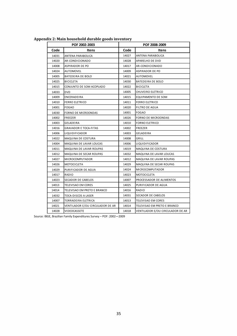
35

Appendix 2: Main household durable goods inventory

Source: IBGE, Brazilian Family Expenditures Survey – POF: 2002—2009

Code Itens Code Itens

14031 ANTENA PARABOLICA 14027 ANTENA PARABOLICA

14020 AR-CONDICIONADO 14028 APARELHO DE DVD

14008 ASPIRADOR DE PO 14017 AR-CONDICIONADO

14024 AUTOMOVEL 14009 ASPIRADOR DE PO

14005 BATEDEIRA DE BOLO 14021 AUTOMOVEL

14025 BICICLETA 14030 BATEDEIRA DE BOLO

14015 CONJUNTO DE SOM ACOPLADO 14022 BICICLETA

14033 DVD 14005 CHUVEIRO ELETRICO

14009 ENCERADEIRA 14015 EQUIPAMENTO DE SOM

14010 FERRO ELETRICO 14011 FERRO ELETRICO

14001 FOGAO 14020 FILTRO DE AGUA

14030 FORNO DE MICROONDAS 14001 FOGAO

14002 FREEZER 14026 FORNO DE MICROONDAS

14003 GELADEIRA 14010 FORNO ELETRICO

14016 GRAVADOR E TOCA-FITAS 14002 FREEZER

14006 LIQUIDIFICADOR 14003 GELADEIRA

14022 MAQUINA DE COSTURA 14008 GRILL

14004 MAQUINA DE LAVAR LOUCAS 14006 LIQUIDIFICADOR

14011 MAQUINA DE LAVAR ROUPAS 14019 MAQUINA DE COSTURA

14012 MAQUINA DE SECAR ROUPAS 14032 MAQUINA DE LAVAR LOUCAS

14027 MICROCOMPUTADOR 14012 MAQUINA DE LAVAR ROUPAS

14026 MOTOCICLETA 14029 MAQUINA DE SECAR ROUPAS

14029 PURIFICADOR DE AGUA 14024 MICROCOMPUTADOR

14017 RADIO 14023 MOTOCICLETA

14023 SECADOR DE CABELOS 14007 PROCESSADOR DE ALIMENTOS

14013 TELEVISAO EM CORES 14025 PURIFICADOR DE AGUA

14014 TELEVISAO EM PRETO E BRANCO 14016 RADIO

14032 TOCA-DISCOS A LASER 14031 SECADOR DE CABELOS

14007 TORRADEIRA ELETRICA 14013 TELEVISAO EM CORES

14021 VENTILADOR E/OU CIRCULADOR DE AR 14014 TELEVISAO EM PRETO E BRANCO

14028 VIDEOCASSETE 14018 VENTILADOR E/OU CIRCULADOR DE AR

POF 2002-2003 POF 2008-2009

36

Appendix 3: Food Items Consumption basket (a) Food Items Consumption basket 2002-2003

Source: IBGE, Brazilian Family Expenditures Survey – POF: 2002—2003

POF CODE Food Items Consumption basket 2002-2003 POF CODE Food Items Consumption basket 2002-2003

1103 Arroz não especificado 7105 Contrafilé

1104 Arroz polido 7201 Acém

1105 Milho em grão 7203 Carne moída

1107 Milho verde em espiga 7204 Carne não especificada

1207 Feijão-preto 7205 Costela

1208 Feijão-rajado 7207 Músculo

1299 Outras leguminosas 7304 Carne moída não especificada

2103 Alface 7399 Outras carnes bovinas outras

2109 Repolho 7503 Mortadela

2201 Abóbora 7506 Presunto

2205 Cebola 7508 Salsicha comum

2206 Chuchu 7603 Lingüiça

2210 Pepino fresco 8103 Fígado

2211 Pimentão 9118 Sardinha em conserva

2213 Tomate 10105 Frango abatido (inteiro)

2301 Alho 11102 Leite condensado

2305 Batata-doce 11104 Leite de vaca pasteurizado

2306 Batata-inglesa 11202 Queijo mozarela

2307 Beterraba 11205 Queijo prato

2309 Cenoura 11301 Iogurte

3111 Banana-prata 11303 Manteiga

3112 Outras bananas 12101 Açúcar cristal

3118 Laranja-pêra 12104 Açúcar refinado

3120 Outras laranjas 12206 Doce de fruta em pasta

3122 Limão comum 12299 Outros doces e produtos de confeitaria

3125 Manga 12301 Chocolate em pó

3127 Melancia 13102 Sal refinado

3204 Maçã 13201 Caldo de carne em tablete

5101 Farinha de mandioca 13202 Caldo de galinha em tablete

5103 Farinha de trigo 13207 Maionese

5104 Farinha vitaminada 13208 Massa de tomate

5201 Amido de milho 13210 Tempero misto

5202 Creme de arroz 13299 Outros condimentos

5208 Fubá de milho 14106 Óleo de soja

5301 Macarrão com ovos 14202 Margarina vegetal

5302 Macarrão não especificado 15103 Cerveja

5303 Macarrão sem ovos 15202 Refrigerante de cola

6108 Pão doce 15203 Refrigerante de guaraná

6109 Pão francês 15204 Refrigerante de laranja

6201 Bolos 15209 Refrigerante não especificado

6301 Biscoito doce 15211 Suco de fruta em pó

6303 Biscoito salgado 15212 Suco de fruta envasado

7101 Alcatra 15301 Café moído

7103 Carne não especificada 16201 Mistura para bolo

7104 Chã-de-dentro

37

Appendix 3: Food Items Consumption basket (b) Food Items Consumption basket 2008-2009

Source: IBGE, Brazilian Family Expenditures Survey – POF: 2008—2009

POF CODE Food Items Consumption basket 2008-2009 POF CODE Food Items Consumption basket 2008-2009

1103 Arroz não especificado e outros 7499 Outras Carnes suinas com osso e sem osso

1104 Arroz polido 7503 Mortadela

1105 Milho em grão 7506 Presunto

1106 Milho verde em conserva 7508 Salsicha comum

1207 Feijão-preto 7511 Toucinho defumado

1299 Outras Lguminosas 7599 Outras carnes suinas outras

2103 Alface 7603 Lingüiça

2105 Cheiro-verde 9118 Sardinha em conserva

2106 Couve 10102 Carne de frango não especificada

2109 Repolho 10103 Coxa de frango

2201 Abóbora 10105 Frango abatido (inteiro)

2205 Cebola 10107 Miúdos de frango

2206 Chuchu 10108 Peito de frango

2211 Pimentão 10201 Ovo de galinha

2213 Tomate 11101 Creme de leite

2301 Alho 11102 Leite condensado

2306 Batata-inglesa 11104 Leite de vaca pasteurizado

2307 Beterraba 11106 Leite em pó integral

2309 Cenoura 11199 Outros Leite e creme de leite

2310 Batata não especificada e outras 11202 Queijo mozarela

2312 Mandioca 11203 Queijo não especificado

3105 Banana-d'água 11205 Queijo prato

3112 Outras bananas 11301 Iogurte

3118 Laranja-pêra 11302 Leite fermentado

3120 Outras laranjas 11303 Manteiga

3124 Mamão 12101 Açúcar cristal

3125 Manga 12201 Bombom

3129 Tangerina 12208 Sorvete

3204 Maçã 12299 Outros Doces e produtos de confeitaria

5101 Farinha de mandioca 12301 Chocolate em pó

5103 Farinha de trigo 13102 Sal refinado

5199 Outras Farinhas 13201 Caldo de carne em tablete

5201 Amido de milho 13202 Caldo de galinha em tablete

5208 Fubá de milho 13203 Outros caldos em tablete

5301 Macarrão com ovos 13207 Maionese

5302 Macarrão não especificado e outros 13208 Massa de tomate

6104 Pão de forma industrializado 13209 Molho de tomate

6108 Pão doce 13299 Outros Condimentos

6109 Pão francês 14101 Azeite de oliva

6110 Pão integral 14106 Óleo de soja

6201 Bolos 14202 Margarina vegetal

6301 Biscoito doce 15104 Vinho

6302 Biscoito não especificado e outros 15201 Água mineral

6303 Biscoito salgado 15202 Refrigerante de cola

7102 Carne moída 15203 Refrigerante de guaraná

7103 Carne não especificada 15204 Refrigerante de laranja

7104 Chã-de-dentro 15209 Refrigerante não especificado

7109 Patinho 15211 Suco de fruta em pó

7201 Acém 15212 Suco de fruta envasado

7203 Carne moída 15301 Café moído

7204 Carne não especificada 16102 Batata frita

7205 Costela 16105 Frango empanado

7304 Carne moída não especificada 16107 Refeição

7305 Carne não especificada 16199 Outros Alimentos preparados

7399 Outras Carnes bovinas outras 16201 Mistura para bolo

38

Appendix 4: Adapt Laspeyres Index

Source: IBGE, Brazilian Family Expenditures Survey – POF: 2002—2009