the existence of solutions for a nonlinear, fractional

University of Nebraska - LincolnDigitalCommons@University of Nebraska - LincolnDissertations, Theses, and Student Research Papersin Mathematics Mathematics, Department of

4-2017

The Existence of Solutions for a Nonlinear,Fractional Self-Adjoint Difference EquationKevin AhrendtUniversity of Nebraska-Lincoln, [email protected]

Follow this and additional works at: http://digitalcommons.unl.edu/mathstudent

Part of the Other Mathematics Commons

This Article is brought to you for free and open access by the Mathematics, Department of at DigitalCommons@University of Nebraska - Lincoln. Ithas been accepted for inclusion in Dissertations, Theses, and Student Research Papers in Mathematics by an authorized administrator ofDigitalCommons@University of Nebraska - Lincoln.

Ahrendt, Kevin, "The Existence of Solutions for a Nonlinear, Fractional Self-Adjoint Difference Equation" (2017). Dissertations, Theses,and Student Research Papers in Mathematics. 79.http://digitalcommons.unl.edu/mathstudent/79

http://digitalcommons.unl.edu?utm_source=digitalcommons.unl.edu%2Fmathstudent%2F79&utm_medium=PDF&utm_campaign=PDFCoverPages

http://digitalcommons.unl.edu/mathstudent?utm_source=digitalcommons.unl.edu%2Fmathstudent%2F79&utm_medium=PDF&utm_campaign=PDFCoverPages


http://digitalcommons.unl.edu/mathematics?utm_source=digitalcommons.unl.edu%2Fmathstudent%2F79&utm_medium=PDF&utm_campaign=PDFCoverPages


http://network.bepress.com/hgg/discipline/185?utm_source=digitalcommons.unl.edu%2Fmathstudent%2F79&utm_medium=PDF&utm_campaign=PDFCoverPages

http://digitalcommons.unl.edu/mathstudent/79?utm_source=digitalcommons.unl.edu%2Fmathstudent%2F79&utm_medium=PDF&utm_campaign=PDFCoverPages

THE EXISTENCE OF SOLUTIONS FOR A NONLINEAR, FRACTIONAL

SELF-ADJOINT DIFFERENCE EQUATION

by

Kevin Ahrendt

A DISSERTATION

Presented to the Faculty of

The Graduate College at the University of Nebraska

In Partial Fulfilment of Requirements

For the Degree of Doctor of Philosophy

Major: Mathematics

Under the Supervision of Professor Allan Peterson

Lincoln, Nebraska

April, 2017

THE EXISTENCE OF SOLUTIONS FOR A NONLINEAR, FRACTIONAL

SELF-ADJOINT DIFFERENCE EQUATION

Kevin Ahrendt, Ph.D.

University of Nebraska, 2017

Adviser: Allan Peterson

In this work we will explore a fractional self-adjoint difference equation which involves

a Caputo fractional difference. In particular, we will develop a Cauchy function for

initial value problems and Green’s functions for several different types of boundary

value problems. We will use the properties of those Green’s functions and the Con-

traction Mapping Theorem to find sufficient conditions for when a nonlinear boundary

value problem has a unique solution. We will also investigate the existence of non-

negative solutions for a nonlinear self-adjoint difference that have particular long run

behavior.

iii

DEDICATION

This dissertation is dedicated to my parents, Randy and Sandi Ahrendt.

iv

ACKNOWLEDGMENTS

I would like to thank my adviser, Allan Peterson, for his constant support starting

when I was an undergraduate at UNL through my graduate school career. He made

this process an enjoyable one, and I always know he cares about me professionally

and personally.

I extend gratitude to my readers Dr. Radu and Dr. Toundykov for there advice

and comments, as well as Dr. Variyam for being on my committee. I also thank the

UNL Mathematics Department for their support over the 10 years I have been here.

I want to especially thank Lori Mueller and Marilyn Johnson for all their help.

I have had the pleasure to work with many fellow graduate students at UNL,

especially the fellow students who have Dr. Peterson as an adviser. Thank you Abby

Brackins, Scott Gensler, Wei Hu, Areeba Ikram, Ariel Setniker, and Julia St. Goar

for many fruitful discussions in the fractional calculus seminar. I have also had the

pleasure to share offices with several other graduate students who provided suppport,

so thank you Andrew Becklin, Jessalyn Bolkema, Michael Brown, Jessica De Silva,

Christina Edholm, Maranda Franke, Lara Ismert, Seth Lindokken, Jason Lutz, Cait-

lyn Parmelee, Peder Thompson, and Marcus Webb. I also appreciate the friendships

I developed in graduate school with Nick Kass, Sara Reynolds, and Andrew Windle.

I want to thank the REU students that I had the pleasure to mentor in the sum-

mer of 2014. Their work contributed heavily to the development of this dissertation.

Thank you Lydia DeWolf, Liam Mazurowski, Kelsey Mitchell, Tim Rolling, and Do-

minic Veconi.

I have had many wonderful math teachers over the years. I especially want to

thank Ken Lindemann for sparking my interest in math and Collin Bleak who made

me realize I wanted to pursue mathematics professionally.

v

My family has provided constant support through good and bad times, so thank

you to my parents Randy and Sandi and my brothers Bryan and Chris. Chris has

been a great mentor in mathematics, and I appreciate all the advice he has given

me. I also want to extend my gratitude to Dr. Rajesh Singh for helping me through

difficult aspects of my life.

Finally, I want to especially thank my partner Areeba Ikram. She has provided

endless support and I appreciate sharing this journey with her.

vi

PREFACE

The history of fractional calculus extends back to 1695 when L’Hopital asked Leibniz

about the nature of a one-half derivative. In the 1800s, Liouville gave a strong

theoretical foundation for studying fractional derivatives leading to the development

of the Riemann-Liouville Definition of a fractional derivative. Caputo later defined

the Caputo fractional derivative, which a form of is studied in this work. See [25] for

a brief history on fractional calculus.

There are many real world applications for the fractional derivative. In the typical

continuous case, fractional calculus can model containment flow in heterogeneous

porous media [11] [12], waves in viscoelastic media [1], and waves in complex media

like biological tissue [29]. In the discrete case, Atici and Sengul [8] use fractional

difference equations to model tumor growth.

The discrete fractional calculus has a domain of a specific time scale. See [13]

and [14] for more results on time scales in the general setting. Whole order difference

equations are studied in detail in [27]. Work in the discrete fractional calculus was

heavily advanced for the delta case in [9] [22] [23]. A broad overview of Discrete

Fractional Calculus is given in [17].

The results in Chapter 1 are mostly well known background material. Section 1.4

contains some new results that will be useful in later proofs. Results in Chapter 2 and

Section 3.1 contain results where the basic problem has been adjusted to fix mistakes

by Ahrendt, et al in [3]. Section 3.2 cites results from [16]. Section 3.3 contains new

work. Finally, Chapter 4’s results are all new.

vii

Table of Contents

1 Introduction to Nabla Fractional Calculus 1

1.1 Basic Results for the Nabla Whole-Order Calculus . . . . . . . . . . . 1

1.1.1 Nabla Difference . . . . . . . . . . . . . . . . . . . . . . . . . 1

1.1.2 Nabla Integral . . . . . . . . . . . . . . . . . . . . . . . . . . . 4

1.2 Extending Results to Fractional Values . . . . . . . . . . . . . . . . . 6

1.3 Nabla Taylor Monomials . . . . . . . . . . . . . . . . . . . . . . . . . 8

1.4 Fractional Taylor monomials . . . . . . . . . . . . . . . . . . . . . . . 9

1.5 Basic Results for the Nabla Fractional Calculus . . . . . . . . . . . . 14

2 Fractional Self-Adjoint Difference Equations 18

2.1 Self-Adjoint Initial Value Problems . . . . . . . . . . . . . . . . . . . 22

2.1.1 Cauchy Function Examples . . . . . . . . . . . . . . . . . . . 28

2.2 Self-Adjoint Boundary Value Problems . . . . . . . . . . . . . . . . . 30

3 Green’s Functions for Specific Boundary Value Problems 42

3.1 A Conjugate Boundary Value Problem . . . . . . . . . . . . . . . . . 42

3.1.1 Conjugate Green’s Function . . . . . . . . . . . . . . . . . . . 43

3.1.2 Conjugate Green’s Function Properties . . . . . . . . . . . . . 45

3.1.3 Graph of Conjugate Green’s Function . . . . . . . . . . . . . . 52

3.2 A Right Focal Boundary Value Problem . . . . . . . . . . . . . . . . 53

viii

3.2.1 Right Focal Green’s Function . . . . . . . . . . . . . . . . . . 53

3.2.2 Right Focal Green’s Function Properties . . . . . . . . . . . . 54

3.2.3 Graph of Right Focal Green’s Function . . . . . . . . . . . . . 54

3.3 A Three Point Boundary Value Problem . . . . . . . . . . . . . . . . 54

3.3.1 Three Point Green’s Function . . . . . . . . . . . . . . . . . . 56

3.3.2 Special Cases of the Three Point Boundary Value Problem . . 61

3.3.3 Three Point Green’s Function Properties . . . . . . . . . . . . 63

3.3.4 Graphs of Three Point Green’s Functions . . . . . . . . . . . . 80

4 Applications of the Contraction Mapping Theorem to Fractional

Self-Adjoint Difference Equations 83

4.1 Long Run Behavior of Equations with Generalized Forcing Terms . . 83

4.1.1 Long Run Behavior Theorem . . . . . . . . . . . . . . . . . . 84

4.1.2 Example . . . . . . . . . . . . . . . . . . . . . . . . . . . . . . 93

4.2 Unique Solutions to Nonlinear Boundary Value Problems . . . . . . . 95

4.2.1 Unique Solutions to a Nonlinear Conjugate BVP . . . . . . . . 96

4.2.1.1 Nonlinear Conjugate BVP Example . . . . . . . . . . 100

4.2.2 Unique Solutions to a Nonlinear Right Focal BVP . . . . . . . 100

4.2.2.1 Nonlinear Right Focal BVP Example . . . . . . . . . 101

4.2.3 Unique Solutions to a Nonlinear Three-Point BVP . . . . . . . 102

4.2.3.1 Nonlinear Right Focal BVP Example . . . . . . . . . 103

Bibliography 104

1

Chapter 1

Introduction to Nabla Fractional Calculus

We will first look at the nabla discrete calculus before going into detail about the

fractional case. A full treatment of the nabla discrete calculus is given in [17, Chapter

3]. Closely related is the delta discrete calculus, which appears heavily in ordinary

difference equations. For more information on ordinary difference equations, see [27].

For the following results we will let a ∈ R be a fixed constant. We will also follow

the convention that b ∈ R such that b − a is a natural number. Then we define the

form of two domains we will be dealing with:

Na := a, a+ 1, a+ 2, . . . and Nba := a, a+ 1, . . . , b− 1, b.

1.1 Basic Results for the Nabla Whole-Order Calculus

1.1.1 Nabla Difference

Definition 1. [17] The backwards jump operator ρ : Na → Na is defined by

ρ(t) := maxa, t− 1.

The backwards jump operator can be loosely thought of as the previous point in

2

the domain.

The analog to the derivative in ordinary real-valued calculus is the nabla difference.

Definition 2. [17] Let f : Na → R. Then the nabla difference of f is defined by

(∇f)(t) := f(t)− f(t− 1),

for t ∈ Na+1. For convenience, we will use the notation ∇f(t) := (∇f)(t). For

N ∈ N2, we have that the N th order fractional difference is recursively defined as

∇Nf(t) := ∇(∇N−1f(t)),

for t ∈ Na+N .

Remark 3. We can reformulate the previous definition in terms of the backwards

jump operator. If f : Na → R, then (∇f)(t) := f(t)− f(ρ(t)) for t ∈ Na+1.

Remark 4. We treat the difference operator of order 0 as the identity operator, i.e.

∇0f(t) = f(t).

With the difference operator in hand, the next theorem shows that the expected

results of derivatives in the typical real case have analogs to the nabla discrete case.

Theorem 5 (Properties of the Nabla Difference). [17] Assume f, g : Na → R and

α, β ∈ R. Then for t ∈ Na+1,

1. ∇α = 0;

2. ∇αf(t) = α∇f(t);

3

3. ∇(f(t) + g(t)) = ∇f(t) +∇g(t);

4. ∇ (f(t)g(t)) = f(ρ(t))∇g(t) +∇f(t)g(t);

5. ∇f(t)g(t)

= g(t)∇f(t)−f(t)∇g(t)g(t)g(ρ(t))

, if g(t) 6= 0 for all t ∈ Na+1.

We also desire a power rule that matches what we would expect in the typical real

case. To do so, we will next define the rising function.

Definition 6. [17] For t ∈ Na and n ∈ N1, the rising function tn is defined as follows:

tn := t(t+ 1)(t+ 2) · · · (t+ n− 1).

We read tn as t to the n rising.

Remark 7. We can reformulate this definition of the rising function using factorial

functions when our domain is based at a = 1. This form will be useful when we

generalize the rising function in the next section. So for t ∈ N1 and n ∈ N1

tn :=(t+ n− 1)!

(t− 1)!.

The rising function as defined gives us a power rule that behaves as expected from

the real-valued calculus case.

Theorem 8 (Nabla Power Rule). [17] For n ∈ N1 and α ∈ R,

∇t(t+ α)n = n(t+ α)n−1,

for t ∈ R.

4

1.1.2 Nabla Integral

Just as we have a derivative operator for the nabla calculus, we have an integral

operator.

Definition 9. [17] Let f : Na → R and let c, d ∈ Na. Then the definite nabla integral

of f from c to d is defined by

∫ d

c

f(s)∇s :=

∑d

s=c+1 f(s), c < d,

0, d ≤ c.

Remark 10. We can think of the nabla integral as a right-hand Riemann sum from

real-valued calculus. Note that∫ baf(s)∇s does not depend on the value of the function

at t = a. Since the nabla integral is defined as a sum, we may say nabla sum in place

of the term nabla integral.

Remark 11. We often use a shorthand notation to represent the nabla integral in a

similar manner as notating the nabla difference. We say

∇−1a f(t) :=

∫ b

a

f(t)∇s.

Here the ‘a’ in ∇−1a f(t) represents the lower limit of the above integral, in which case

we say the integral is based at a. The ‘−1’ represents taking the nabla integral, where

the negative sign indicates we are doing the opposite operation of a nabla difference.

We can extend this to other integer values where

∇−na f(t) :=

∫ t

a

∫ τ1

a

∫ τ2

a

· · ·∫ τn−1

a

f(τn)∇τn∇τn−1 · · · ∇τ2∇τ1.

This notation will be used for integration and differentiation of fractional orders.

5

The next theorem gives properties of the nabla integral, all of which have an

analogous result in the real-valued calculus.

Theorem 12 (Properties of the Nabla Integral). [17] Assume f, g : Na+1 → R,

b, c, d ∈ Na such that b ≤ c ≤ d, and α ∈ R. Then

1.∫ cbαf(t)∇t = α

∫ cbf(t)∇t;

2.∫ cb(f(t) + g(t))∇t =

∫ cbf(t)∇t+

∫ cbg(t)∇t;

3.∫ dbf(t)∇t =

∫ cbf(t)∇t+

∫ dcf(t)∇t;

4.∣∣∫ cbf(t)∇(t)

∣∣ ≤ ∫ cb|f(t)|∇t;

5. If F (t) :=∫ tbf(s)∇s, for t ∈ Nc

b, then ∇F (t) = f(t), t ∈ Ncb+1;

6. If f(t) ≥ g(t) for t ∈ Ncb+1, then

∫ cbf(t)∇t ≥

∫ cbg(t)∇t.

Definition 13 (Nabla Antidifference). [17] Assume f : Nba+1 → R. We say F : Nb

a →

R is a nabla antidifference of f(t) on Nba provided

∇F (t) = f(t),

for t ∈ Nba+1.

Theorem 14 (Fundamental Theorem of Nabla Calculus). [17] Assume the function

f : Nba → R and let F be a nabla antidifference of f on Nb

a, then

∫ b

a

f(t)∇t = F (t)

∣∣∣∣ba

:= F (b)− F (a).

The following Leibniz rules are very useful.

6

Theorem 15 (Leibniz Formulas). [17] Assume f : Na × Na+1 → R. Then, for

t ∈ Na+1,

∇(∫ t

a

f(t, τ)∇τ)

=

∫ t

a

∇tf(t, τ)∇τ + f(ρ(t), t), (1.1)

and

∇(∫ t

a

f(t, τ)∇τ)

=

∫ t−1

a

∇tf(t, τ)∇τ + f(t, t). (1.2)

In the case where the limits of integration are constant, we can interchange the

order of the nabla operator and integration operator.

Theorem 16 (Leibniz Formula with Constant Limits of Integration). Assume f :

Na × Na+1 → R. Then, for t ∈ Na+1,

∇(∫ b

a

f(t, τ)∇τ)

=

∫ b

a

∇tf(t, τ)∇τ.

1.2 Extending Results to Fractional Values

We want to extend some of the previous results to the fractional case. For example,

we can consider a nabla integral of order 1.2 or a nabla difference of order π. To do

so, we need to define the Gamma function.

Definition 17. [30] The gamma function is defined by the integral

Γ(z) =

∫ ∞0

e−ttz−1dt,

for z ∈ C\. . . ,−2,−1, 0.

One of the most useful results of the gamma function that we will frequently use

is that it behaves like the factorial function, i.e. Γ(t + 1) = tΓ(t). Furthermore, if

n ∈ N1, then Γ(n) = (n−1)!, following the convention that 0! = 1. For this reason, we

7

say that the Gamma function generalizes the factorial function beyond nonnegative

integers.

Since the Gamma function extends the factorial function to values in

C\. . . ,−2,−1, 0, it is natural to extend the definition of the rising function as

follows, using the form from Remark 7.

Definition 18. [17] Let t ∈ R and let n ∈ N1. Then the rising function is defined by

tn := (t)(t+ 1) · · · (t+ n− 1) =Γ(t+ n)

Γ(t),

where Γ is the gamma function. For ν ∈ R, the generalized rising function is then

defined by

tν :=Γ(t+ ν)

Γ(t)

for t and ν such that t+ ν 6∈ . . . ,−2,−1, 0. If t is a non-positive integer and t+ ν

is not a non-positive integer then we take by convention tν = 0.

The power rule still holds in this more generalized case.

Theorem 19 (Generalized Power Rules). [17] For values of t, r, and α so that the

values in the following equations make sense as per Definition 18, we have that

∇(t+ α)r = r(t+ α)r−1,

and

∇(α− t)r = −r(α− ρ(t))r−1.

We can also take integrals of the rising functions, getting a generalized power rule

for integrals.

8

Theorem 20 (Power Rules for the Nabla Integral). [17]

1.∫

(t− α)r∇t = 1r+1

(t− α)r+1 + C, r 6= −1;

2.∫

(α− ρ(t))r∇t = − 1r+1

(α− t)r+1+C, r 6= −1.

1.3 Nabla Taylor Monomials

In this section we will state the definition of the Nabla Taylor monomials in both the

whole order case along with several properties.

Definition 21. For n ∈ N0, we define the nabla Taylor monomials by H0(t, a) := 1

for t ∈ Na, and

Hn(t, a) =(t− a)n

n!, for t ∈ Na−n+1, when n ∈ N1.

Theorem 22 (Properties of Taylor Monomials). [17] The nabla Taylor monomials

satisfy the following properties:

1. Hn(t, a) = 0, for t ∈ Naa−n+1 and n ∈ N1;

2. ∇Hn+1(t, a) = Hn(t, a), for t ∈ Na−n+1 and n ∈ N0;

3. ∇sHn+1(t, s) = −Hn(t, ρ(s)), for t ∈ Ns;

4.∫ taHn(τ, a)∇τ = Hn+1(t, a), for t ∈ Na and n ∈ N0;

5.∫ taHn(t, ρ(s))∇s = Hn+1(t, a), for t ∈ Na and n ∈ N0.

Theorem 23 (Discrete Whole-Order Taylor’s Formula). [5] Fix N ∈ N1 and let

f : Na−N+1 → R. Then

f(t) =N−1∑k=0

∇kf(a)Hk(t, a) +

∫ t

a

HN−1(t, ρ(s))∇Nf(s)∇s,

9

for t ∈ Na.

1.4 Fractional Taylor monomials

In this section, we will extend the definition of Taylor monomials to fractional values

using the Gamma function. We will also state and prove some properties of the

fractional Taylor monomial that will prove useful in later chapters.

Definition 24. [17] Let µ 6= −1,−2,−3, · · · . Then we define the µ-th order nabla

fractional Taylor monomoial Hµ(t, a) by

Hµ(t, a) :=(t− a)µ

Γ(µ+ 1),

for values of t ∈ R such that the right hand side makes sense. By convention, if t− a

is a non-positive integer, but t−a+µ is not a non-positive integer, then Hν(t, a) := 0.

Theorem 25 (Properties of Fractional Taylor Monomials). [17] The following hold:

1. Hµ(a, a) = 0,

2. ∇Hµ(t, a) = Hµ−1(t, a),

3. ∇Hµ(t, s) = −Hµ−1(t, ρ(s)),

4.∫ taHµ(s, a)∇s = Hµ+1(t, a),

5.∫ taHµ(t, ρ(s))∇s = Hµ+1(t, a),

6. H−k(t, a) = 0, for k ∈ N1 and t ∈ Na,

provided the expressions used are well defined.

Lemma 26. For −1 < µ < 0, we have that limt→∞ tµ = 0.

10

Proof. We will first consider limt→∞tµ

Γ(µ+1). Then, for t ∈ N1,

tµ

Γ(µ+ 1)=

Γ(t+ µ)

Γ(t)Γ(µ+ 1)

=(µ+ 1)t−1

Γ(t)

=(µ+ 1)(µ+ 2) · · · (µ+ t− 1)

(t− 1)!

=

(µ+ 1

1

)(µ+ 2

2

)· · ·(µ+ t− 1

t− 1

)=

t−1∏n=1

µ+ n

n

=t−1∏n=1

(1 +

µ

n

).

So we then have that limt→∞tµ

Γ(µ+1)=∏∞

n=1

(1 + µ

n

). Note here that −1 < µ

n< 0 for

all n ∈ N1, so this infinite product is well defined. But we then have

∞∏n=1

(1 +

µ

n

)= exp

(∞∑n=1

ln(

1 +µ

n

)).

We claim∑∞

n=1 ln(1 + µ

n

)diverges to−∞. To see this, we will show

∑∞n=1− ln

(1 + µ

n

)diverges to ∞ by applying the integral test, i.e. we consider the limit

limb→∞

∫ b

1

− ln(

1 +µ

x

)dx.

Note that − ln(1 + µ

x

)> 0 for all x ∈ [1,∞), − ln

(1 + µ

x

)is decreasing with respect

to x on [1,∞), and − ln(1 + µ

x

)is continuous with respect to x on [1,∞), thus we

11

can apply the integral test. We will integrate∫ b

1− ln

(1 + µ

x

)dx by parts.

∫ b

1

− ln(

1 +µ

x

)dx =

(− ln

(1 +

µ

x

)x)|bx=1 −

∫ b

1

µx

µx+ x2dx

= − ln(

1 +µ

b

)b+ ln(1 + µ)− (µ ln |µ+ x|) |bx=1

= − ln(

1 +µ

b

)b+ ln(1 + µ)− µ ln(µ+ b) + µ ln(µ+ 1).

Consider then

limb→∞− ln

(1 +

µ

b

)b = lim

b→∞

− ln(1 + µ

b

)1b

= limb→∞

µµb+b2

− 1b2

= limb→∞− µb

µ+ b= −µ,

after applying L’Hopital’s rule.

Also,

limb→∞−µ ln(µ+ b) =∞,

as µ < 0.

Thus

limb→∞− ln

(1 +

µ

x

)dx

= limb→∞

[− ln

(1 +

µ

b

)b+ ln(1 + µ)− µ ln(µ+ b) + µ ln(µ+ 1)|

]=∞.

Therefore, by the integral test,∑∞

n=1− ln(1 + µ

n

)diverges to ∞, thus∑∞

n=1 ln(1 + µ

n

)diverges to −∞. Hence

limt→∞

tµ

Γ(µ+ 1)= exp

(∞∑n=1

ln(

1 +µ

n

))= 0.

12

Finally, since limt→∞tµ

Γ(µ+1)= 0, we get that 1

Γ(µ+1)limt→∞ t

µ = 0, hence

limt→∞

tµ = 0.

Lemma 27. For t ∈ Na, s ∈ Nta, and µ > −1, we have

Hµ(t, s) ≥ 0.

Proof. First note if t = s, then by convention Hµ(t, s) = 0. So consider t ∈ Na+1 and

s ∈ Nt−1a . Then

Hµ(t, s) :=(t− s)µ

Γ(µ+ 1)=

Γ(t− s+ µ)

Γ(t− s)Γ(µ+ 1).

By our assumption on t and s, we have that t−s ∈ N1. So t−s+µ > 0 and t−s > 0

implying Γ(t − s + µ) > 0 and Γ(t − s) > 0. Finally, µ > −1, so µ + 1 > 0, which

implies Γ(µ+ 1) > 0. Hence for t ∈ Na+1 and s ∈ Nt−1a , Hµ(t, s) > 0.

Lemma 28. For −1 < µ < 0, t ∈ Na+2, and s ∈ Nta+2, we have that

∇sHµ(t, ρ(s)) ≥ 0.

13

Proof. For s ∈ Nta+2, consider

∇sHµ(t, ρ(s)) =∇s(t− ρ(s))µ

Γ(µ+ 1)

=∇s(t+ 1− s)µ

Γ(µ+ 1)

= −(µ)(t+ 1− ρ(s))µ−1

Γ(µ+ 1)

= −(µ)Γ(t+ 1− s+ 1 + µ− 1)

Γ(t+ 1− s+ 1)(µ)Γ(µ)

= − Γ(t− s+ µ+ 1)

Γ(t− s+ 2)Γ(µ).

Since s ∈ Nta+2, we have that Γ(t − s + µ + 1) > 0 and Γ(t − s + 2) > 0. Since

−1 < µ < 0, Γ(µ) < 0. Thus ∇sHµ(t, ρ(s)) ≥ 0.

Lemma 29. For µ ∈ R such that µ is not a non-positive integer, s ∈ Na and t ∈ Ns+1,

we have

Hµ(t, ρ(s)) =

(µ+ 1

t− s

)Hµ+1(t, s).

Proof. Consider

Hµ(t, ρ(s)) :=(t− ρ(s))µ

Γ(µ+ 1)

Def. 18=

Γ(t− s+ 1 + µ)

Γ(t− s+ 1)Γ(µ+ 1)

=Γ(t− s+ (µ+ 1))

(t− s)Γ(t− s)Γ(µ+ 1)·(µ+ 1

µ+ 1

)=

(µ+ 1

t− s

)Γ(t− s+ (µ+ 1))

Γ(t− s)Γ(µ+ 2)

=

(µ+ 1

t− s

)Hµ+1(t, s).

14

1.5 Basic Results for the Nabla Fractional Calculus

A full discussion of the nabla discrete fractional calculus is in [17, Chapter 3]. Some

of the originating results are from [21]. These results have analogs to results in the

study of the real fractional calculus. For more information about fractional calculus

in the real case, see [30].

Definition 30. [21] Let f : Na+1 → R, ν > 0. The νth order nabla fractional sum of

f is defined by

∇−νa f(t) :=

∫ t

a

Hν−1(t, ρ(s))f(s)∇s,

for t ∈ Na.

We define the Riemann-Liouville nabla fractional difference in terms of a whole

order nabla difference and a nabla fractional sum.

Definition 31. [21] Let f : Na → R, ν > 0, and N := dνe. Then νth order Riemann-

Liouville nabla fractional difference of f is defined as

∇νaf(t) := ∇N∇−(N−ν)

a f(t),

for t ∈ Na+N .

While we will mostly focus on the Caputo fractional difference given in the up-

coming Definition 35, the Riemann-Liouville difference is useful for intermediate steps

in certain proofs. In particular, the following composition rules will be useful.

Theorem 32 (Composition Rules). [2, Theorem 6.1] Let µ > 0, ν > 0, and let

f : Na → R. Define N := dνe. Then

∇−νa ∇−µa f(t) = ∇−ν−µa f(t), t ∈ Na,

15

and

∇νa∇−µa f(t) = ∇ν−µ

a f(t), t ∈ Na+N .

The following specific composition rule is also useful; it enables us to effectively

cancel out Riemann-Liouville differences and sums through composition.

Theorem 33. [17, Corollary 3.122] For 0 < µ < 1 and f : Na+1 → R, we have that

∇−µa ∇µaf(t) = f(t),

for t ∈ Na+1.

It will prove useful later to consider nabla fractional sums consisting of an integral

of a function with two variables with constant limits of integration.

Lemma 34. Let c ∈ Na, d ∈ Nc, and µ > 0 be given. Assume f : Na × Nc+1 → R.

Then, for t ∈ Na,

∇−µa(∫ d

c

f(t, τ)∇τ)

=

∫ d

c

∇−µa f(t, τ)∇τ.

Proof. For t ∈ Na, consider

∇−µa(∫ d

c

f(t, τ)∇τ)

=

∫ t

a

Hµ−1(t, ρ(s))

∫ d

c

f(s, τ)∇τ∇s

=t∑

s=a+1

d∑τ=c+1

Hµ−1(t, ρ(s))f(s, τ)

=d∑

τ=c+1

t∑s=a+1

Hµ−1(t, ρ(s))f(s, τ)

=

∫ d

c

∫ t

a

Hµ−1(t, ρ(s))f(s, τ)∇s∇τ

=

∫ d

c

∇−µa f(t, τ)∇τ.

16

The following definition has been adapted from Anastassiou in [4].

Definition 35. Let f : Na−N+1 → R, ν > 0, ν ∈ R, and N := dνe. The νth order

Caputo nabla fractional difference is defined as

∇νa∗f(t) := ∇−(N−ν)

a (∇Nf(t)),

for t ∈ Na+1. Note that the Caputo difference operator is a linear operator.

Remark 36. Note the difference between the Caputo fractional difference and the

Riemann-Liouville fractional difference is the order of the composition of the fractional

sum and whole order difference.

The following lemma shows Caputo fractional difference has some particularly

nice behavior as a consequence of the order discussed in Remark 36.

Lemma 37. [3, Lemma 15] Let 0 < ν < 1 and let x : Na → R. Then

∇νa∗x(a+ 1) = ∇x(a+ 1).

It will be useful later to consider Caputo fractional sums of an integral of a function

with two variables with constant limits of integration.

Lemma 38. Let c ∈ Na, d ∈ Nc, and ν > 0 be given. Assume f : Na−N+1×Nc+1 → R

and take N = dνe. Then for t ∈ Na+1,

∇νa∗

(∫ d

c

f(t, τ)∇τ)

=

∫ d

c

∇νa∗f(t, τ)∇τ.

17

Proof. For t ∈ Na+1,

∇νa∗

(∫ d

c

f(t, τ)∇τ)

= ∇−(N−ν)a ∇N

(∫ d

c

f(t, τ)∇τ)

= ∇−(N−ν)a

(∫ d

c

∇Nt f(t, τ)∇τ

)=

∫ d

c

∇−(N−ν)a ∇N

t f(t, τ)∇τ, (by Theorem 16)

=

∫ d

c

∇νa∗f(t, τ)∇τ, (by Lemma 34).

18

Chapter 2

Fractional Self-Adjoint Difference Equations

In the continuous setting, let D := x : x and px′ are continuously differentiable on R.

Then the second-order formally self-adjoint operator on D is given by

(Lx)(t) := [p(t)x′(t)]′ + q(t)x(t),

where p : R → (0,∞) and q : R → R. This operator has importance in functional

analysis (see [24, Chapter 10]) for more details. It also has applications in theoretical

physics [6]. Many equivalent results to this chapter in the continuous setting is given

in [26, Chapter 5].

The self-adjoint operator studied here for the discrete fractional case follows. Let

Da := x : Na → R and let the fractional self-adjoint operator La be defined by

(Lax)(t) := ∇[p(t)∇νa∗x(t)] + q(t)x(t− 1), t ∈ Na+2,

where x ∈ Da, 0 < ν < 1, p : Na+1 → (0,∞) such that p(t) 6= p(a+1)H−ν(t,a)

for some

t ∈ Na+1, and q : Na+2 → R. Note that La is a linear operator.

Remark 39 (Domain of x, p, and q in the self-adjoint operator). The operator is

defined for t ∈ Na+2, but x(t) is defined for t ∈ Na. This is a result of the Caputo

19

fractional derivative only being defined on Na+1, (see Definition 35), and so then the

whole order nabla difference of the Caputo fractional derivative is only defined on

Na+2 (see Definition 2).

For the domains of p and q, consider the following expansion of the self-adjoint

operator

(Lax)(t) = ∇[p(t)∇νa∗x(t)] + q(t)x(t− 1)

= ∇[p(t)∇−(1−ν)

a ∇x(t)]

+ q(t)x(t− 1)

= ∇[p(t)

∫ t

a

H−ν(t, ρ(s)) [x(s)− x(s− 1)]∇s]

+ q(t)x(t− 1)

= p(t)

∫ t

a

H−ν(t, ρ(s)) [x(s)− x(s− 1)]∇s

− p(t− 1)

∫ t−1

a

H−ν(t− 1, ρ(s)) [x(s)− x(s− 1)]∇s+ q(t)x(t− 1)

= p(t)H−ν(t, ρ(t)) [x(t)− x(t− 1)]

+ p(t)

∫ t−1

a

H−ν(t, ρ(s)) [x(s)− x(s− 1)]∇s

− p(t− 1)

∫ t−1

a

H−ν(t− 1, ρ(s)) [x(s)− x(s− 1)]∇s+ q(t)x(t− 1)

= p(t) [x(t)− x(t− 1)]

+ p(t)

∫ t−1

a

H−ν(t, ρ(s)) [x(s)− x(s− 1)]∇s

− p(t− 1)

∫ t−1

a

H−ν(t− 1, ρ(s)) [x(s)− x(s− 1)]∇s+ q(t)x(t− 1)

= p(t)x(t) + [q(t)− p(t)]x(t− 1)

+ p(t)

∫ t−1

a

H−ν(t, ρ(s)) [x(s)− x(s− 1)]∇s

− p(t− 1)

∫ t−1

a

H−ν(t− 1, ρ(s)) [x(s)− x(s− 1)]∇s.

Since the operator is defined for t ∈ Na+2, the above expansion shows that p(t) only

20

needs to be defined for t ∈ Na+1 and q(t) only needs to be defined for t ∈ Na+2.

Remark 40. The restriction that p(t) 6= p(a+1)H−ν(t,a)

for some t ∈ Na+1 will guarantee

unique solutions to initial value problems involving the self-adjoint operator (see

Theorem 43).

The fractional self-adjoint difference equation behaves similar to a second order

difference equation. For instance, a general solution to the homogeneous equation

is given by a linear combination of two linearly independent solutions. Note the

following theorem relies on the existence and uniqueness of self-adjoint initial value

problems, which is given in Theorem 43 in the next section.

Theorem 41 (General Solution of the Homogeneous Equation). Suppose x1, x2 :

Na → R are linearly independent solutions to Lax(t) = 0. Then a general solution to

Lax(t) = 0 is given by

x(t) = c1x1(t) + c2x2(t),

for t ∈ Na, where c1, c2 ∈ R are arbitrary constants.

Proof. Let x1(t) and x2(t) be two linearly independent solutions to Lax(t) = 0, and

let c1 and c2 be arbitrary constants. Then define x(t) := c1x1(t) + c2x2(t). Since La

is a linear operator, we have that

Lax(t) = c1Lax1(t) + c2Lax2(t) = c1 · 0 + c2 · 0 = 0,

hence x(t) = c1x1(t) + c2x(t) solves Lax(t) = 0 for any constants c1 and c2.

We now claim that any solution x(t) to Lax(t) = 0 can be written uniquely in the

form of x(t) = c1x1(t) + c2x2(t) for suitable constants c1 and c2. Since x1 : Na → R

21

and x2 : Na → R, we have that there exists constants α, β, γ, and δ ∈ R such that

x1(a) = α, ∇x1(a+ 1) = β, x2(a) = γ, and ∇x2(a+ 1) = δ.

Let x : Na → R be any arbitrary function that solves Lax(t) = 0. As before, there

exists constants A and B such that x(a) = A and ∇x(a+ 1) = B. Hence x(t) solves

the initial value problem

Lax(t) = 0, t ∈ Na+2,

x(a) = A, ∇x(a+ 1) = B.

Consider the vector equation

x1(a) x2(a)

∇x1(a+ 1) ∇x2(a+ 1)

c1

c2

=

AB

. (2.1)

Note this is equivalent to

α γ

β δ

c1

c2

=

AB

.

We claim that there exists unique c1, c2 ∈ R that satisfy the above matrix equation.

By way of contradiction, suppose not. Then

∣∣∣∣∣∣∣α γ

β δ

∣∣∣∣∣∣∣ = 0.

Then, without lost of generality, there exists a constant k ∈ R such that α = kγ

and β = kδ. Relabelling, we get that x1(a) = α = kγ = kx2(a) and ∇x1(a + 1) =

β = kδ = k∇x2(a + 1). But kx2(t) solve Lax(t) = 0, as La is a linear operator, and

22

from before Lax1(t) = 0. Hence kx2(t) and x1(t) satisfy the same difference equation

and the same initial conditions, hence by the uniqueness of solutions initial value

problems (see Theorem 43) x1(t) = kx2(t) for t ∈ Na. This implies x1(t) and x2(t)

are linearly dependent on Na, which is a contradiction. Hence the vector equation

(2.1) has a unique solution, so x(t) and c1x1(t) + c2x2(t) solve the same initial value

problem, hence every solution to Lax(t) = 0 can be expressed uniquely as a linear

combination of x1(t) and x2(t).

The proof of the following result is straight forward.

Corollary 42 (General Solution of the Nonhomogeneous Equation). Suppose x1, x2 :

Na → R are linearly independent solutions of Lax(t) = 0 and xp : Na → R is a

particular solution to Lax(t) = h(t) for some h : Na+2 → R. Then a general solution

of Lax(t) = h(t) is given by

x(t) = c1x1(t) + c2x2(t) + xp(t),

for t ∈ Na, and where c1, c2 ∈ R are arbitrary constants.

2.1 Self-Adjoint Initial Value Problems

Theorem 43 (Existence and Uniqueness for Self-Adjoint IVPs). Let A,B ∈ R, and

h : Na+2 → R and assume p(t) 6= p(a+1)H−ν(t,a)

for all t ∈ Na+2. Then the initial value

problem Lax(t) = h(t), t ∈ Na+2,

x(a) = A, ∇x(a+ 1) = B,

(2.2)

has a unique solution x : Na → R.

23

Proof. Define x(t) to satisfy the initial conditions in (2.2). It follows that

x(a) = A, x(a+ 1) = A+B,

and then for t ∈ Na+2, define

x(t) :=1

p(t)

[h(t)−

([q(t)− p(t)]x(t− 1) + p(t)

t−1∑s=a+1

H−ν(t, ρ(s)) [x(s)− x(s− 1)]

−p(t− 1)t−1∑

s=a+1

H−ν(t− 1, ρ(s)) [x(s)− x(s− 1)]

)].

(2.3)

For any fixed t ∈ Na+2, we have that the coefficient of the x(a) term in (2.3) is given

by − [p(t)H−ν(t, a)− p(t− 1)H−ν(t− 1, a)] = −∇ [p(t)H−ν(t, a)] . For x(t), with t ∈

Na+2, to be uniquely determined by the initial conditions, we need that the coefficient

of x(a) is nonzero for some t ∈ Na+2. So to avoid the situation of∇ [p(t)H−ν(t, a)] = 0,

we must have p(t) 6= CH−ν(t,a)

, where C ∈ R is an arbitrary constant. In particular,

we can define C := p(a+ 1), so then we must have p(t) 6= p(a+1)H−ν(t,a)

for some t ∈ Na+2,

which is one of our assumptions. Therefore there exists some t ∈ Na+2 such that x(t)

depends on the initial condition x(a) = A. See Remark 44 for why there is no issue

regarding the coefficient of x(a+ 1).

Note that when t = a+2, x(a+2) depends only on the known functions p(t), q(t),

and h(t), as well as x(a) and x(a+1). Hence x(a+2) is uniquely determined from the

known functions and the initial conditions. Then for t = a+ 3, we have that x(a+ 3)

depends only on the known functions p(t), q(t), and h(t), as well as x(a), x(a + 1),

and x(a + 2). Hence x(a + 3) is uniquely determined by the known functions and

the previous values of x. Continuing on in this fashion, we get that x(t) is uniquely

24

determined by p(t), q(t), h(t), and x(s) for s = a, a + 1, . . . , t − 1. Thus for t ∈ Na,

x(t) is uniquely defined by the initial conditions and the recursion equation. (2.3).

Consider the following rearrangement of (2.3) using integral notation instead of

summation notation,

p(t)x(t) + [q(t)− p(t)]x(t− 1)

+ p(t)

∫ t−1

a

H−ν(t, ρ(s)) [x(s)− x(s− 1)]∇s

− p(t− 1)

∫ t−1

a

H−ν(t− 1, ρ(s)) [x(s)− x(s− 1)]∇s

= h(t).

(2.4)

Here the left hand side of the above equation is simply the expanded form of the

self-adjoint operator given in Remark 39, hence x(t) as defined above satisfies the

initial conditions and the self-adjoint equation

Lax(t) = ∇[p(t)∇νa∗x(t)] + q(t)x(t) = h(t).

Therefore x(t) uniquely solves (2.2).

Remark 44. For t ∈ Na+3, we have that the coefficient of x(a+ 1) is given by

p(t) [H−ν(t, a)−H−ν(t, a+ 1)]− p(t− 1) [H−ν(t− 1, a)−H−ν(t− 1, a+ 1)]

= ∇ [p(t) (H−ν(t, a)−H−ν(t, a+ 1))]

= ∇ [p(t) (H−ν(t, a)−H−ν(t− 1, a))]

= ∇ [p(t)H−ν−1(t, a)] .

The coefficient of x(a + 1) needs to be nonzero for some t ∈ Na+3, which requires

p(t) 6= CH−ν−1(t,a)

for all t ∈ Na+3 and for some constant C ∈ R. In particular, if

25

we take C = p(a + 1), we require p(t) 6= p(a+1)H−ν−1(t,a)

for all t ∈ Na+3. Recall that

p : Na+1 → (0,∞), so p(a + 1) > 0. However, H−ν−1(t, a) < 0 for t ∈ Na+2, thus the

condition that p is a positive valued function already avoids the possible issue of the

coefficient of x(a+ 1) being zero for all t ∈ Na+2.

Definition 45. The Cauchy function for Lax(t) = 0 is the function x(t, s), where

x : Na × Na+2 → R, which for any fixed s ∈ Na+2, satisfies the initial value problem

Lρ(s)x(t, s) = 0, t ∈ Ns+1

x(ρ(s), s) = 0,

∇x(s, s) = 1p(s)

.

(2.5)

Theorem 46 (Variation of Constants). Let h : Na+2 → R. Then the solution to the

initial value problem Lax(t) = h(t), t ∈ Na+2,

x(a) = 0

∇x(a+ 1) = 0,

(2.6)

is given by

x(t) =

∫ t

a+1

x(t, s)h(s)∇s,

where x(t, s) is the Cauchy function for the homogeneous equation.

Proof. Define x(t) :=∫ ta+1

x(t, s)h(s)∇s, where x(t, s) is the Cauchy function for

Lax(t) = 0. Note that x(a) =∫ aa+1

x(a, s)h(s)∇s = 0 by convention and x(a + 1) =∫ a+1

a+1x(a+ 1, s)h(s)∇s = 0. Hence ∇x(a+ 1) = x(a+ 1)− x(a) = 0, thus the initial

conditions are satisfied.

26

Now consider

∇[p(t)∇ν

ρ(s)∗x(t, s)]

= ∇[p(t)∇−(1−ν)

ρ(s) ∇tx(t, s)]

= ∇[p(t)∇−(1−ν)

ρ(s) (x(t, s)− x(t− 1, s))]

= ∇[p(t)

∫ t

ρ(s)

H−ν(t, ρ(τ)) (x(τ, s)− x(τ − 1, s))∇τ].

(2.7)

Using Leibniz’s Formula (1.1), we have

∇ [p(t)∇νa∗x(t)] = ∇

[p(t)∇−(1−ν)

a ∇x(t)]

= ∇[p(t)∇−(1−ν)

a ∇∫ t

a+1

x(t, s)h(s)∇s]

= ∇[p(t)∇−(1−ν)

a

(∫ t

a+1

∇tx(t, s)h(s)∇s+ x(ρ(t), t)h(t)

)]= ∇

[p(t)∇−(1−ν)

a

∫ t

a+1

∇tx(t, s)h(s)∇s],

where we used the first initial condition in the definition of the Cauchy function.

Continuing this expansion, we get

∇ [p(t)∇νa∗x(t)] = ∇

[p(t)∇−(1−ν)

a

∫ t

a+1

∇tx(t, s)h(s)∇s]

= ∇[p(t)∇−(1−ν)

a

∫ t

a+1

(x(t, s)− x(t− 1, s))h(s)∇s]

= ∇[p(t)

∫ t

a

H−ν(t, ρ(τ))

∫ τ

a+1

(x(τ, s)− x(τ − 1, s))h(s)∇s∇τ]

= ∇

[p(t)

t∑τ=a+1

τ∑s=a+2

H−ν(t, ρ(τ)) (x(τ, s)− x(τ − 1, s))h(s)

],

using the sum definition of the nabla integral. By interchanging the order of summa-

tion, applying Leibniz’s formula (1.2), using both initial conditions in the definition

27

of the Cauchy function, and using (2.7), we get

∇ [p(t)∇νa∗x(t)] = ∇

[p(t)

t∑s=a+2

h(s)t∑

τ=s

H−ν(t, ρ(τ)) (x(τ, s)− x(τ − 1, s))

]

=t−1∑

s=a+2

(h(s)∇t

[p(t)

t∑τ=s

H−ν(t, ρ(τ)) (x(τ, s)− x(τ − 1, s))

])

+ h(t)p(t)H−ν(t, ρ(t)) (x(t, t)− x(t− 1, t))

=

∫ t−1

a+1

(h(s)

· ∇t

[p(t)

∫ t

ρ(s)

H−ν(t, ρ(τ)) (x(τ, s)− x(τ − 1, s))∇τ])∇s

+ h(t)p(t)

(1

p(t)− 0

)= h(t) +

∫ t−1

a+1

h(s)(∇[p(t)∇ν

ρ(s)∗x(t, s)])∇s.

So finally,

Lax(t) = ∇ [p(t)∇νa∗x(t)] + q(t)x(t− 1)

= h(t) +

∫ t−1

a+1

h(s)(∇[p(t)∇ν

ρ(s)∗x(t, s)])∇s+ q(t)

∫ t−1

a+1

x(t− 1, s)h(s)∇s

= h(t) +

∫ t−1

a+1

h(s)(∇[p(t)∇ν

ρ(s)∗x(t, s)]

+ q(t)x(t− 1, s))∇s

= h(t) +

∫ t−1

a+1

h(s)Lρ(s)x(t, s)∇s

= h(t).

Hence x(t) =∫ ta+1

x(t, s)h(s) solves the initial value problem (2.6).

Theorem 47 (Variation of Constants with Non-Zero Initial Conditions). Let h :

28

Na+2 → R. Then the solution to the initial value problem

Lax(t) = h(t), t ∈ Na+2,

x(a) = A,

∇x(a+ 1) = B,

where A,B ∈ R are arbitrary constants, is given by

x(t) = x0(t) +

∫ t

a+1

x(t, s)h(s)∇s,

where x0(t) solves the initial value problem

Lax0(t) = 0, t ∈ Na+2,

x0(a) = A,

∇x0(a+ 1) = B.

Proof. This proof follows from the linearity of the self-adjoint operator.

2.1.1 Cauchy Function Examples

Example 48. Find the Cauchy function for ∇ [p(t)∇νa∗x(t)] = 0.

For fixed s ∈ Na+1, we consider the initial value problem

∇[p(t)∇ν

ρ(s)∗x(t, s)]

= 0, t ∈ Ns+1,

x(ρ(s), s) = 0,

∇x(s, s) = 1p(s)

.

Integrating the above difference equation on both sides from s to t and using the

29

Fundamental Theorem of Nabla Calculus yields

p(t)∇νρ(s)∗x(t, s)− p(s)∇ν

ρ(s)∗x(s, s) = 0.

By Lemma 37 and the second initial condition in the definition of the Cauchy function,

this is equivalent to

p(t)∇νρ(s)∗x(t, s)− p(s)∇x(s, s) = p(t)∇ν

ρ(s)∗x(t, s)− p(s) 1

p(s)= 0,

hence

∇νρ(s)∗x(t, s) = ∇−(1−ν)

ρ(s) ∇x(t, s) =1

p(t).

By composing both sides with the operator ∇1−νρ(s) , we get that

∇x(t, s) = ∇1−νρ(s)

1

p(t).

Using Theorem 32, we get

∇x(t, s) = ∇∇−νρ(s)

1

p(t)= ∇

∫ t

ρ(s)

Hν−1(t, ρ(τ))1

p(τ)∇τ,

and so by integrating from ρ(s) to t and using the Fundamental Theorem of Nabla

Calculus,

x(t, s)− x(ρ(s), s) =

∫ t

ρ(s)

Hν−1(t, ρ(τ))1

p(τ)∇τ −

∫ ρ(s)

ρ(s)

Hν−1(ρ(s), ρ(τ))1

p(τ)∇τ.

Then by the first initial condition in the definition of the Cauchy function and by

30

convention on nabla integrals, we get

x(t, s) =

∫ t

ρ(s)

Hν−1(t, ρ(τ))1

p(τ)∇τ = ∇−νρ(s)

1

p(t).

Example 49. Find the Cauchy function for ∇∇νa∗x(t) = 0. Note this is a specific

case of Example 48 where p(t) ≡ 1. Hence

x(t, s) = ∇−νρ(s)1

=

∫ t

ρ(s)

Hν−1(t, ρ(τ))∇τ

= −Hν(t, τ)|tτ=ρ(s)

= Hν(t, ρ(s)).

Hence the Cauchy function for ∇∇νa∗x(t) = 0 is given by x(t, s) = Hν(t, ρ(s)).

2.2 Self-Adjoint Boundary Value Problems

In this section we develop techniques to solve boundary value problems for the frac-

tional self-adjoint operator involving the Caputo difference. See Brackins [15] for a

similar development using the Riemann-Liouville definition of a fractional difference.

In the continuous setting, [28] has some work on boundary value problems involv-

ing fractional derivatives. Some work in the delta case on fractional boundary value

problems is given in [19]. In [7], they develop Green’s functions in the delta case.

31

We are interested in the homogeneous self-adjoint boundary value problem

Lax(t) = 0, t ∈ Nb

a+2,

αx(a)− β∇x(a+ 1) = 0,

γx(b) + δ∇x(b) = 0,

(2.8)

and the corresponding nonhomogeneous self-adjoint boundary value problem

Lax(t) = h(t), t ∈ Nb

a+2,

αx(a)− β∇x(a+ 1) = A,

γx(b) + δ∇x(b) = B,

(2.9)

where 0 < ν < 1; b− a ∈ N2; α, β, γ, δ, A, and B are real-valued constants such that

α2 + β2 > 0 and γ2 + δ2 > 0; and h : Nba+2 → R. Note that the difference equation

is satisfied only for t ∈ Nba+2, but solutions to these boundary value problems are

defined on Nba.

Theorem 50. Assume (2.8) has only the trivial solution. Then (2.9) has a unique

solution.

Proof. Let x1, x2 : Na → R be two linearly independent solutions of Lax(t) = 0.

Then by Theorem 41, a general solution is given by x(t) = c1x1(t) + c2x2(t), where

c1, c2 ∈ R are arbitrary constants. Note that x(t) satisfies the boundary conditions

in (2.8) if it satisfies the following system of equations

α [c1x1(a) + c2x2(a)]− β∇ [c1x1(a+ 1) + c2x2(a+ 1)] = 0,

γ [c1x1(b) + c2x2(b)] + δ∇ [c1x1(b) + c2x2(b)] = 0,

32

if and only if it satisfies the following equivalent system of equations

c1 [αx1(a)− β∇x1(a+ 1)] + c2 [αx2(a)− β∇x2(a+ 1)] = 0,

c1 [γx1(b) + δ∇x1(b)] + c2 [γx2(b) + δ∇x2(b)] = 0,

which is equivalent to the following vector equation

αx1(a)− β∇x1(a+ 1) αx2(a)− β∇x2(a+ 1)

γx1(b) + δ∇x1(b) γx2(b) + δ∇x2(b)

c1

c2

=

0

0

.

But x(t) is the trivial solution if and only if c1 = c2 = 0 if and only if

D :=

∣∣∣∣∣∣∣αx1(a)− β∇x1(a+ 1) αx2(a)− β∇x2(a+ 1)

γx1(b) + δ∇x1(b) γx2(b) + δ∇x2(b)

∣∣∣∣∣∣∣ 6= 0.

Hence if (2.8) has only the trivial solution, then D 6= 0.

Now consider (2.9). By Corollary 42, a general solution to Lax(t) = h(t) is given

by x(t) = a1x1(t) + a2x2(t) + xp(t), where a1, a2 ∈ R are arbitrary constants and

xp(t) : Na → R is a particular solution to Lax(t) = h(t). To satisfy the boundary

conditions in (2.9), x(t) must satisfy the following system of equations

α [a1x1(a) + a2x2(a)]− β∇ [a1x1(a+ 1) + a2x2(a+ 1)]

= A− αxp(a) + β∇xp(a+ 1),

γ [a1x1(b) + a2x2(b)] + δ∇ [a1x1(b) + a2x2(b)]

= B − γxp(b)− δ∇xp(b),

33

if and only if it satisfies the following equivalent system of equations

a1 [αx1(a)− β∇x1(a+ 1)] + a2 [αx2(a)− β∇x2(a+ 1)]

= A− αxp(a) + β∇xp(a+ 1),

a1 [γx1(b) + δ∇x1(b)] + a2 [γx2(b) + δ∇x2(b)]

= B − γxp(b)− δ∇xp(b),

which is equivalent to the following vector equation

αx1(a)− β∇x1(a+ 1) αx2(a)− β∇x2(a+ 1)

γx1(b) + δ∇x1(b) γx2(b) + δ∇x2(b)

a1

a2

=

A− αxp(a) + β∇xp(a+ 1)

B − γxp(b)− δ∇xp(b)

.

But from before, D 6= 0, hence there exists unique a1, a2 ∈ R such that the above

matrix equation is satisfied. Hence x(t) = a1x1(t) + a2x2(t) + xp(t) uniquely solves

the nonhomogeneous boundary value problem (2.9).

Theorem 51. Let r := αγ(∇−νa 1

p(t)

)|t=b + αδ

(∇1−νa

1p(t)

)|t=b + βγ

p(a+1). Then the

boundary value problem

∇ [p(t)∇ν

a∗x(t)] = 0, t ∈ Nba+2,

αx(a)− β∇x(a+ 1) = 0,

γx(b) + δ∇x(b) = 0,

(2.10)

has only the trivial solution if and only if r 6= 0.

Proof. Note that x1(t) = 1 and x2(t) = ∇−νa 1p(t)

are two linearly independent solutions

34

to ∇ [p(t)∇νa∗x(t)] = 0, so by Theorem 41 a general solution to ∇ [p(t)∇ν

a∗x(t)] = 0

is given by x(t) = c1 + c2∇−νa 1p(t)

, where c1, c2 ∈ R are arbitrary constants. Consider

the left boundary condition

αx(a)− β∇x(a+ 1) = α

[c1 + c2∇−νa

1

p(t)

]|t=a − β

[c1∇1 + c2∇∇−νa

1

p(t)

]|t=a+1

= c1α− c2β

(∇1−νa

1

p(t)

)|t=a+1

= c1α− c2β

∫ a+1

a

Hν−2(a+ 1, ρ(s))1

p(s)∇s

= c1α− c2β

p(a+ 1)

= 0.

Hence c1 and c2 satisfy c1α−c2β

p(a+1)= 0. Now consider the right boundary condition

γx(b) + δ∇x(b) = γ

[c1 + c2∇−νa

1

p(t)

]|t=b + δ

[c1∇1 + c2∇∇−νa

1

p(t)

]|t=b

= c1γ + c2γ

(∇−νa

1

p(t)

)|t=b + c2δ

(∇1−νa

1

p(t)

)|t=b

= 0.

Hence c1 and c2 satisfy c1γ + c2

[γ(∇−νa 1

p(t)

)|t=b + δ

(∇1−νa

1p(t)

)|t=b]

= 0.

Using these boundary conditions, c1 and c2 must satisfy the following vector equa-

tion α − βp(a+1)

γ γ(∇−νa 1

p(t)

)|t=b + δ

(∇1−νa

1p(t)

)|t=b

c1

c2

=

0

0

.

35

Note then the determinant of the previous matrix is given by

∣∣∣∣∣∣∣α − β

p(a+1)

γ γ(∇−νa 1

p(t)

)|t=b + δ

(∇1−νa

1p(t)

)|t=b

∣∣∣∣∣∣∣ = αγ

(∇−νa

1

p(t)

)|t=b + αδ

(∇1−νa

1

p(t)

)|t=b

+βγ

p(a+ 1)

= r,

thus the boundary value problem (2.10) has only the trivial solution if and only if

r 6= 0.

Example 52 (Non-unique BVP Solution). The following boundary value problem

does not have a unique solution.

∇[∇ν

a∗x(t)] = h(t), t ∈ Nba+2,

∇x(a+ 1) = A,

∇x(b) = B.

To see this, note this BVP is a specific case of (2.10) where α = 0, β = −1, γ = 0,

δ = 1, and p(t) ≡ 1. Then

r := αγ

(∇−νa

1

p(t)

)|t=b + αδ

(∇1−νa

1

p(t)

)|t=b +

βγ

p(a+ 1)= 0.

Hence the above boundary value problem does not have a unique solution by Theorem

51.

Definition 53 (Green’s Function). Assume that (2.8) has only the trivial solution.

We define the Green’s function G(t, s) where G : Nba×Nb

a+2 → R for the homogeneous

36

boundary value problem (2.8) by

G(t, s) :=

u(t, s), t ∈ Nb−1

a and s ∈ Nbmaxt+1,a+2,

v(t, s), t ∈ Nba+1 and s ∈ Nmint+1,b

a+2 ,

where, for each fixed s ∈ Nba+2, u(t, s) solves the boundary value problem

Lau(t, s) = 0, t ∈ Nb

a+2

αu(a, s)− β (∇tu(t, s)) |t=a+1 = 0,

γu(b, s) + δ (∇tu(t, s)) |t=b = − [γx(b, s) + δ (∇tx(t, s)) |t=b] ,

and v(t, s) := u(t, s) + x(t, s), where x(t, s) is the Cauchy function for Lax(t) = 0.

Remark 54. Note some care is needed when specifying domains for u(t, s) and v(t, s)

while respecting the domains for the t and s components of the Green’s function. For

example, in the case of u(t, s), if t = a, then t+ 1 = a+ 1, but t+ 1 = a+ 1 6∈ Nba+2,

which is the domain for s. Hence we use maxt+ 1, a+ 2 for the lower bound on the

domain of s. Also for the case of u(t, s), when t = b, we would have s ∈ Nbb+1, which

is an impossible situation. Hence we restrict the domain of t to be in Nb−1a . Similarly,

the upper bound for the domain of s in the definition of v(t, s) is mint + 1, b and

the lower bound for the domain of t is a+ 1.

Remark 55. When dealing with the Green’s function defined piecewise, there is an

overlap of the domains for u(t, s) and v(t, s) when s = t+ 1. The Green’s function is

still well defined, as u(t, s) = v(t, s) when s = t+ 1. To see this, note

v(t, t+ 1) := u(t, t+ 1) + x(t, t+ 1) = u(t, t+ 1) + 0 = u(t, t+ 1),

37

where x(t, s) is the Cauchy function for Lax(t) = 0.

Theorem 56 (Green’s Function Theorem). Assume (2.8) has only the trivial solu-

tion. Then the solution to the nonhomogeneous boundary value problem (2.9), with

A = B = 0, is given by

x(t) =

∫ b

a+1

G(t, s)h(s)∇s,

where G(t, s) is the Green’s function for the homogeneous boundary value problem

(2.8).

Proof. Assume (2.8) has only the trivial solution and consider, for t ∈ Nba+1,

x(t) =

∫ b

a+1

G(t, s)h(s)∇s

=

∫ t

a+1

v(t, s)h(s)∇s+

∫ b

t

u(t, s)h(s)∇s

=

∫ t

a+1

[u(t, s) + x(t, s)]h(s)∇s+

∫ b

t

u(t, s)h(s)∇s

=

∫ b

a+1

u(t, s)h(s)∇s+

∫ t

a+1

x(t, s)h(s)∇s.

(2.11)

When t = a, we have

x(a) =

∫ b

a+1

G(a, s)h(s)∇s

=

∫ b

a+1

u(a, s)h(s)∇s+ 0

=

∫ b

a+1

u(a, s)h(s)∇s+

∫ a

a+1

x(a, s)h(s)∇s

=

(∫ b

a+1

u(t, s)h(s)∇s+

∫ t

a+1

x(t, s)h(s)∇s)|t=a.

(2.12)

38

Hence for t ∈ Nba,

x(t) =

∫ b

a+1

u(t, s)h(s)∇s+

∫ t

a+1

x(t, s)h(s)∇s.

Note that by the variation of constants formula given in Theorem 46,

z(t) :=∫ ta+1

x(t, s)h(s)∇s solves the initial value problem

Laz(t) = h(t), t ∈ Na+2

z(a) = 0,

∇z(a+ 1) = 0.

Thus x(t) =∫ ba+1

u(t, s)h(s)∇s+ z(t). Using Theorem 16 and Lemma 38, composing

both sides of the previous equation with the operator La gives

Lax(t) = La

∫ b

a+1

u(t, s)h(s)∇s+ Laz(t)

= La

∫ t

a+1

u(t, s)h(s)∇s+ La

∫ b

t

u(t, s)h(s)∇s+ h(t)

=

∫ b

a+1

Lau(t, s)h(s)∇s+ h(t)

=

∫ b

a+1

0 · h(s)∇s+ h(t)

= h(t).

Hence x(t) satisfies the difference equation in the nonhomogeneous boundary value

problem (2.9).

39

Now consider the left boundary condition

αx(a)− β∇x(a+ 1) = α

[∫ b

a+1

u(a, s)h(s)∇s+ z(a)

]− β

(∇[∫ b

a+1

u(t, s)h(s)∇s+ z(t)

])|t=a+1

=

∫ b

a+1

αu(a, s)h(s)∇s+ αz(a)

−∫ b

a+1

β (∇tu(t, s)) |t=a+1h(s)∇s− β (∇z(t)) |t=a+1

=

∫ b

a+1

[αu(a, s)− β (∇tu(t, s)) |t=a+1]h(s)∇s

+ [αz(a)− β∇z(a+ 1)]

=

∫ b

a+1

0 · h(s)∇s+ α · 0− β · 0

= 0.

Hence the left boundary condition in (2.9) is satisfied.

40

For the right boundary condition, consider

γx(b) + δ∇x(b) = γ

[∫ b

a+1

u(b, s)h(s)∇s+ z(b)

]+ δ

(∇[∫ b

a+1

u(t, s)h(s)∇s+ z(t)

])|t=b

=

∫ b

a+1

γu(b, s)h(s)∇s+ γz(b)

+

∫ b

a+1

δ (∇tu(t, s))) |t=bh(s)∇s+ δ (∇z(t)) |t=b

=

∫ b

a+1

[γu(b, s) + δ (∇tu(t, s))t=b]h(s)∇s

+ γz(b) + δ (∇z(t)) |t=b

=

∫ b

a+1

[γu(b, s) + δ (∇tu(t, s)) |t=b]h(s)∇s

+ γ

∫ b

a+1

x(b, s)h(s)∇s+ δ

(∇t

∫ b

a+1

x(t, s)h(s)∇s)|t=b

=

∫ b

a+1

[γu(b, s) + δ (∇tu(t, s)) |t=b]h(s)∇s

+

∫ b

a+1

[γx(b, s) + δ (∇tx(t, s)) |t=b]h(s)∇s

=

∫ b

a+1

− [γx(b, s) + δ (∇tx(t, s)) |t=b]h(s)∇s

+

∫ b

a+1

[γx(b, s) + δ (∇tx(t, s)) |t=b]h(s)∇s

= 0.

Thus the right boundary condition in (2.9) is satisfied. Therefore

x(t) =

∫ b

a+1

G(t, s)h(s)∇s

solves the nonhomogeneous boundary value problem (2.9) with A = B = 0.

41

Remark 57. If at the start of the proof we instead consider t ∈ Nb−1a , we would split

the Green’s function into two integrals at the point t+ 1 instead of t as in (2.11) and

considered the t = b case separately in place of (2.12). This would result in the same

end result as a consequence of Remark 55.

Corollary 58. Assume that (2.8) has only the trivial solution. Then the solution to

the nonhomogeneous boundary value problem (2.9), with arbitrary A,B ∈ R, is given

by

x(t) = w(t) +

∫ b

a+1

G(t, s)h(s)∇s,

where G(t, s) is the Green’s function for the homogeneous boundary value problem

(2.8), and w(t) solves the boundary value problem

Law(t) = 0, Nb

a+2,

αw(a)− β∇w(a+ 1) = A,

γw(b) + δ∇w(b) = B.

Proof. The proof follows immediately from Theorem 56 and the linearity of the op-

erator La.

42

Chapter 3

Green’s Functions for Specific Boundary Value Problems

In this chapter, we will continue to look at the fractional self-adjoint difference equa-

tion

∇[p(t)∇νa∗x(t)] + q(t)x(t− 1) = h(t), t ∈ Nb

a+2,

with various boundary conditions.

3.1 A Conjugate Boundary Value Problem

In this section, we investigate the Green’s function for a conjugate boundary value

problem, called as such because the boundary conditions only depend on x at a

and b. Similar results hold in the continuous setting (see [26]). Also, Brackins [15]

investigates a conjugate, fractional, self-adjoint boundary value problem involving the

Riemann-Liouville fractional difference.

In particular, we consider the Green’s function for the conjugate, fractional, self-

adjoint boundary value problem

∇∇ν

a∗x(t) = 0, t ∈ Nba+2,

x(a) = 0,

x(b) = 0.

(3.1)

43

3.1.1 Conjugate Green’s Function

Here we determine the Green’s function for the conjugate, fractional, self-adjoint

boundary value problem (3.1).

Note here that this is a specific case of the general homogeneous boundary value

problem (2.8) where q(t) ≡ 0 and p(t) ≡ 1, with α = 1, β = 0, γ = 1, and δ = 0.

Since

r := αγ

(∇−νa

1

p(t)

)|t=b + αδ

(∇1−νa

1

p(t)

)|t=b +

βγ

p(a+ 1)

= (∇νa1)|t=b + 0 + 0

=

∫ b

a

Hν−1(b, ρ(s)) · 1∇s

= Hν(b, a)

6= 0,

by Theorem 51, (3.1) has only the trivial solution, thus we apply Definition 53, i.e.

we want to, for each fixed s ∈ Nba+2, solve the boundary value problem

∇∇ν

a∗u(t, s) = 0, t ∈ Nba+2

u(a, s) = 0,

u(b, s) = −x(b, s) = −Hν(b, ρ(s)),

(3.2)

where x(t, s) = Hν(t, ρ(s)) is the Cauchy function for∇∇νa∗x(t) = 0 found in Example

49.

As in the proof of Theorem 51, x1(t) = 1 and x2(t) = ∇−νa 1 are two linearly

44

independent solutions to Lax(t) = 0. Hence a general solution to (3.2) is given by

u(t, s) = c1(s) + c2(s)∇−νa 1.

Since (∇−νa 1) (t) = Hν(t, a), we have that u(t, s) = c1(s) + c2(s)Hν(t, a). Applying

the first boundary condition, we get that

u(a, s) = c1(s) + c2(s)Hν(a, a) = c1(s) = 0.

Thus u(t, s) = c2(s)Hν(t, a). Applying the second boundary condition gives

u(b, s) = c2(s)Hν(b, a) = −Hν(b, ρ(s)).

Hence c2(s) = −Hν(b,ρ(s))Hν(b,a)

, and therefore

u(t, s) = −Hν(b, ρ(s))Hν(t, a)

Hν(b, a),

which from Definition 53 implies

v(t, s) = −Hν(b, ρ(s))Hν(t, a)

Hν(b, a)+Hν(t, ρ(s)).

Therefore the Green’s function for (3.1) is given by

G(t, s) =

−Hν(b,ρ(s))Hν(t,a)

Hν(b,a), t ∈ Nb−1


−Hν(b,ρ(s))Hν(t,a)Hν(b,a)

+Hν(t, ρ(s)), t ∈ Nba+1 and s ∈ Nmint+1,b

a+2 .

45

3.1.2 Conjugate Green’s Function Properties

Lemma 59. The Green’s function for the boundary value problem (3.6) satisfies

∇tG(t, s) ≤ 0, (3.3)

for t ∈ Nb−1a+1 and s ∈ Nb

t+1, and

∇tG(t, s) ≥ 0, (3.4)

for t ∈ Nba+2 and s ∈ Nt

a+2.

Proof of (3.3): Let t ∈ Nb−1a+1 and s ∈ Nb

t+1. Then G(t, s) = u(t, s). Thus consider

∇tG(t, s) = ∇tu(t, s)

= ∇t

(−Hν(b, ρ(s))Hν(t, a)

Hν(b, a)

)= −Hν(b, ρ(s))Hν−1(t, a)

Hν(b, a).

Since 0 < ν < 1, we have ν > −1 and ν − 1 > −1. So by Lemma 27, we have

Hν(b, ρ(s)) > 0, Hν−1(t, a) > 0, and Hν(b, a) > 0. Hence, for t ∈ Nb−1a+1 and s ∈ Nb

t+1,

∇tG(t, s) ≤ 0.

Proof of (3.4): Let t ∈ Nba+2 and s ∈ Nt

a+2. Then G(t, s) = v(t, s), so

∇tG(t, s) = ∇tv(t, s)

= −∇tHν(b, ρ(s))Hν(t, a)

Hν(b, a)+∇tHν(t, ρ(s))

= −Hν(b, ρ(s))Hν−1(t, a)

Hν(b, a)+Hν−1(t, ρ(s))

46

This is nonnegative if and only if

Hν(b, ρ(s))Hν−1(t, a)

Hν(b, a)≤ Hν−1(t, ρ(s)). (3.5)

Since s ∈ Nta+2 and 0 < ν < 1, we have that t− ρ(s) > 0 implying Hν−1(t, ρ(s)) >

0, so (3.5) is equivalent to

Hν(b, ρ(s))Hν−1(t, a)

Hν(b, a)Hν−1(t, ρ(s))≤ 1

Breaking this down, consider

Hν(b, ρ(s))

Hν(b, a)=

(b− ρ(s))ν

Γ(ν + 1)· Γ(ν + 1)

(b− a)ν

=Γ (b− ρ(s) + ν)

Γ (b− ρ(s))· Γ(b− a)

Γ(b− a+ ν)

=Γ (b− ρ(s) + ν)

Γ(b− a+ ν)· Γ(b− a)

Γ (b− ρ(s)).

Using the property that Γ(x+ 1) = xΓ(x), we can rewrite the previous equality as

Γ (b− ρ(s) + ν)

Γ(b− a+ ν)

Γ(b− a)

Γ (b− ρ(s))

=Γ(b− ρ(s) + ν)

(b− (a+ 1) + ν)Γ(b− (a+ 1) + ν)· (b− (a+ 1))Γ(b− (a+ 1))

Γ(b− ρ(s))

=Γ(b− ρ(s) + ν)

(b− (a+ 1) + ν)(b− (a+ 2) + ν)Γ(b− (a+ 2) + ν)

· (b− (a+ 1))(b− (a+ 2))Γ(b− (a+ 2))

Γ(b− ρ(s))

=Γ(b− ρ(s) + ν)

(b− (a+ 1) + ν)(b− (a+ 2) + ν) · · · (b− ρ(s) + ν)Γ(b− ρ(s) + ν)

· (b− (a+ 1))(b− (a+ 2)) · · · (b− ρ(s))Γ(b− ρ(s))

Γ(b− ρ(s))

=(b− (a+ 1))(b− (a+ 2)) · · · (b− ρ(s))

(b− (a+ 1) + ν)(b− (a+ 2) + ν) · · · (b− ρ(s) + ν).

47

Note that this is shown in general using the · · · notation for multiplication of de-

creasing factors, but may not make sense for small s. However this is not an issue,

because s ∈ Nta+2, the above Gamma property expansions will have at least one term,

i.e. if, at its worst, s = a+ 2, then

Hν(b, ρ(s))

Hν(b, a)=

(b− (a+ 1))

(b− (a+ 1) + ν).

For large s in the domain, the above expansions using shorthand for decreasing factors

will make sense as written.

Since 0 < ν < 1, we get that b−(a+1)b−(a+1)+ν

≤ 1, b−(a+2)b−(a+2)+ν

≤ 1, . . . , b−ρ(s)b−ρ(s)+ν

≤ 1, hence

Hν(b,ρ(s))Hν(b,a)

≤ 1.

By a similar expansion with the same notation issue noted, we get

Hν−1(t, a)

Hν−1(t, ρ(s))=

(t− a+ ν)(t− a+ ν + 1) · · · (t− ρ(s) + ν − 1)

(t− a+ 1)(t− a+ 2) · · · (t− ρ(s)).

Again, since 0 < ν < 1, we have that t−a+νt−a+1

≤ 1, t−a+ν+1t−a+2

≤ 1, . . . , t−ρ(s)+ν−1t−ρ(s)

≤ 1,

thus Hν−1(t,a)Hν−1(t,ρ(s))

≤ 1.

Combining these two results, we get that Hν(b,ρ(s))Hν−1(t,a)Hν(b,a)Hν−1(t,ρ(s))

≤ 1, i.e. (3.5) is true.

Hence ∇tG(t, s) ≥ 0 for t ∈ Nba+2 and s ∈ Nt

a+2.

Remark 60. For Lemma 59, we note that again care must be taken when specifying

the domain of t and s.

If t ∈ Nb−1a and s ∈ Nb

maxt+1,a+2, then G(t, s) = u(t, s). But consider ∇tu(t, s) =

u(t, s)−u(t−1, s). The term u(t−1, s) is defined for t ∈ Nba+1 and s ∈ Nb

maxt,a+2. So

for u(t, s) and u(t−1, s) to be both well defined, we must have t ∈ Nb−1a ∩Nb

a+1 = Nb−1a+1

and s ∈ Nbmaxt+1,a+2∩Nb

maxt,a+2 = Nbmaxt+1,a+2. Since t ∈ Nb−1

a+1, maxt+1, a+2 =

t+ 1. Hence the domain for ∇tu(t, s) is t ∈ Nb−1a+1 and s ∈ Nb

t+1.

48

In the other case, if t ∈ Nba+1 and s ∈ Nmint+1,b

a+2 , then G(t, s) = v(t, s). But

∇tv(t, s) = v(t, s) − v(t − 1, s). The term v(t − 1, s) is defined for t ∈ Nba+2 and

s ∈ Nmint,ba+2 . Therefore, for v(t, s) and v(t − 1, s) to be both well defined, we must

have t ∈ Nba+1 ∩ Nb

a+2 = Nba+2 and s ∈ Nmint+1,b

a+2 ∩ Nmint,ba+2 = Nmint,b

a+2 . But since

t ∈ Nba+2, mint, b = t. Therefore the domain for ∇tv(t, s) is t ∈ Nb

a+2 and s ∈ Nta+2.

Theorem 61. The Green’s function for the boundary value problem

∇∇ν

a∗x(t) = 0, t ∈ Nba+2,

x(a) = 0,

x(b) = 0,

(3.6)

where b− a ∈ N2 and 0 < ν < 1, given by

G(t, s) =






a+2 .

satisfies the inequalities

1. G(t, s) ≤ 0, for t ∈ Nba and s ∈ Nb

a+2,

2. G(t, s) ≥ − (b−a)2

4(b−a)νΓ(ν+1), for t ∈ Nb

a and s ∈ Nba+2,

3.∫ ba+1|G(t, s)|∇s ≤ (b−a)2

4Γ(ν+2), for t ∈ Nb

a,

First we prove a lemma that will simplify the proof of Theorem 61.

Lemma 62. Let t ∈ N1 and 0 < ν < 1. Then

tν ≤ t.

49

Proof. Since t ∈ N1, we have that by properties of the Gamma function

tν =Γ(t+ ν)

Γ(t)≤ Γ(t+ 1)

Γ(t)=tΓ(t)

Γ(t)= t.

Proof of Theorem 61 part (1): Let t ∈ Nb−1a and s ∈ Nb

maxt+1,a+2. Then G(t, s) =

u(t, s). From (3.3), we know that u(t, s) is nonincreasing in t. thus the maximum of

u(t, s) will occur when t = a. So

u(a, s) = −Hν(b, ρ(s))Hν(a, a)

Hν(b, a)= 0,

hence u(t, s) ≤ 0 when t ∈ Nb−1a and s ∈ Nb

maxt+1,a+2.

Let t ∈ Nba+1 and s ∈ Nmint+1,b

a+2 , so then G(t, s) = v(t, s). By (3.4), v(t, s) is

a nondecreasing function in t. Thus the maximum of v(t, s) will occur when t = b.

Consider

v(b, s) = −Hν(b, ρ(s))Hν(b, a)

Hν(b, a)+Hν(b, ρ(s)) = −Hν(b, ρ(s)) +Hν(b, ρ(s)) = 0.

Thus v(t, s) ≤ 0 for all t ∈ Nba+1 and s ∈ Nmint+1,b

a+2 , thus showing G(t, s) ≤ 0 for

t ∈ Nba and s ∈ Nb

a+2.

Proof of Theorem 61 part (2): By Lemma 59, we have that the minimum of the

50

Green’s function occurs when t = ρ(s). So

G(t, s) ≥ G(ρ(s), s)

= −Hν(b, ρ(s))Hν(ρ(s), a)

Hν(b, a)

= −(b− ρ(s))ν

Γ(ν + 1)

Γ(ν + 1)

(b− a)ν(ρ(s)− a)ν

Γ(ν + 1).

But s ∈ Nba+2, so b− ρ(s) ∈ N1 and ρ(s)− a ∈ N1, thus by Lemma 62, we have

G(t, s) ≥ −(b− ρ(s))(ρ(s)− a)

(b− a)νΓ(ν + 1)= −(b− s+ 1)(s− 1− a)

(b− a)νΓ(ν + 1).

But −(b − s + 1)(s − 1 − a) is a parabola opening upwards with roots of s = a + 1

and s = b+ 1 which has its minimum value at s = (a+1)+(b+1)2

= a+b2

+ 1, so

G(t, s) ≥ −(b−

(a+b

2+ 1)

+ 1) ((

a+b2

+ 1)− 1− a

)(b− a)νΓ(ν + 1)

= −(b2− a

2

)( b

2− a

2)

(b− a)νΓ(ν + 1)

= − (b− a)2

4(b− a)νΓ(ν + 1).

51

Proof of Theorem 61 part (3): Part (1) shows that G(t, s) ≤ 0, hence

∫ b

a+1

|G(t, s)|∇s = −∫ b

a+1

G(t, s)∇s

= −∫ t

a+1

v(t, s)∇s−∫ b

t

u(t, s)∇s

= −∫ t

a+1

[u(t, s) + x(t, s)]∇s−∫ b

t

u(t, s)∇s

= −∫ b

a+1

u(t, s)∇s−∫ t

a+1

x(t, s)∇s

=

∫ b

a+1

Hν(b, ρ(s))Hν(t, a)

Hν(b, a)∇s−

∫ t

a+1

Hν(t, ρ(s)∇s.

Applying Theorem 25 to integrate yields

∫ b

a+1

|G(t, s)|∇s =Hν+1(b, a+ 1)Hν(t, a)

Hν(b, a)−Hν+1(t, a+ 1)

= Hν(t, a)(b− a− 1)ν+1

Γ(ν + 2)

Γ(ν + 1)

(b− a)ν− (t− a− 1)ν+1

Γ(ν + 2)

=Hν(t, a)

ν + 1

Γ(b− a− 1 + ν + 1)

Γ(b− a− 1)

Γ(b− a)

Γ(b− a+ ν)

− Γ(t− a− 1 + ν + 1)

Γ(t− a− 1)Γ(ν + 2)

=Hν(t, a)

ν + 1(b− a− 1)− Γ(t− a+ ν)(t− a− 1)

Γ(t− a)(ν + 1)Γ(ν + 1)

=(t− a)ν

(ν + 1)Γ(ν + 1)(b− a− 1)− (t− a)ν

(ν + 1)Γ(ν + 1)(t− a− 1)

=(t− a)ν

Γ(ν + 2)[(b− a− 1)− (t− a− 1)]

=(t− a)ν(b− t)

Γ(ν + 2).

When t = a we get that∫ ba+1|G(t, s)|∇s = 0, so let t ∈ Nb

a+1. Then, since 0 < ν < 1

and t−a ∈ N1, we have that by Lemma 62 (t−a)ν ≤ (t−a). Thus∫ ba+1|G(t, s)|∇s ≤

(t−a)(b−t)Γ(ν+2)

for t ∈ Nba+1. Note that the numerator is a parabola opening downwards

52

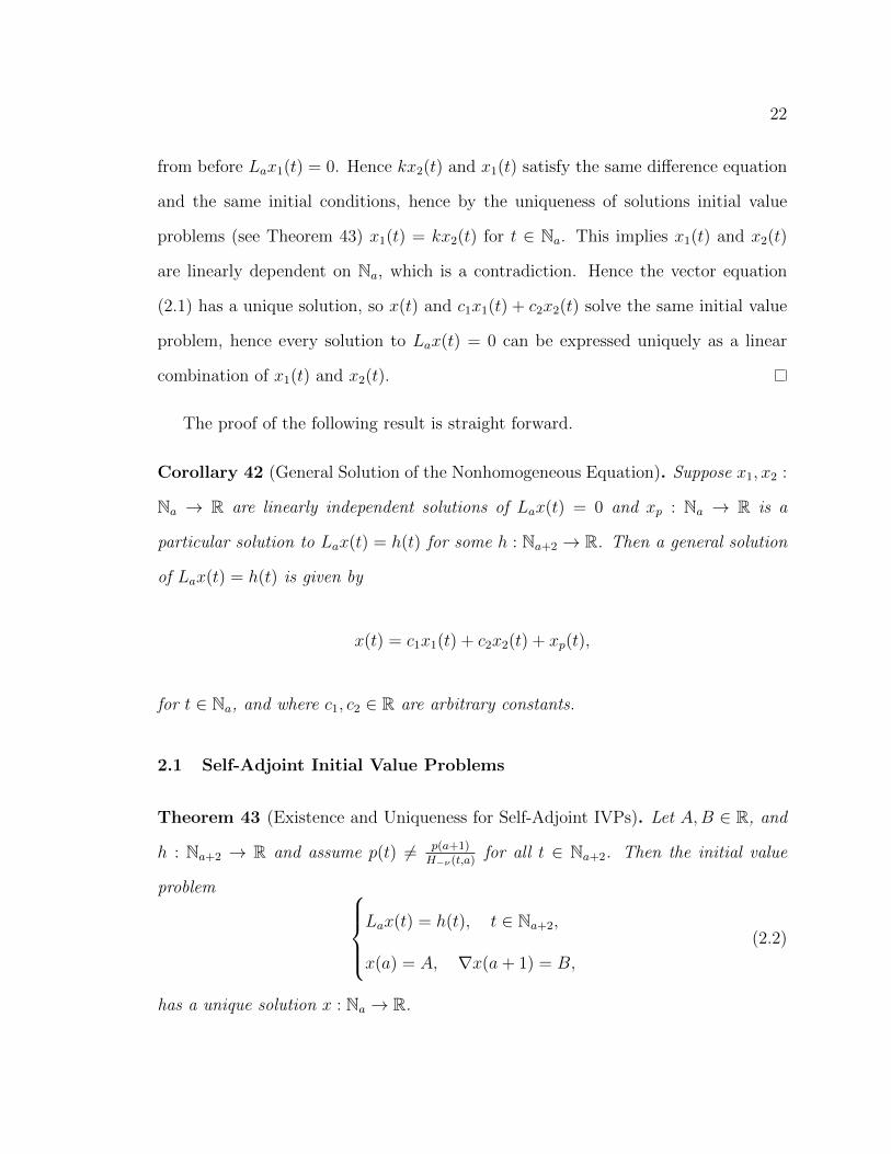
2 4 6 8 10 12 14t

-1.5

-1.0

-0.5

GHt,7L

Figure 3.1: Conjugate Green’s Function as a function of t where b = 15, a = 0,ν = 0.4 and fixed s = 7.

with its maximum value at t = a+b2

. Hence

(t− a)(b− t)Γ(ν + 2)

≤(a+b

2− a)(b− a+b

2)

Γ(ν + 2)=

(b− a)2

4Γ(ν + 2).

Therefore∫ ba+1|G(t, s)|∇s ≤ (b−a)2

4Γ(ν+2), for all t ∈ Nb

a.

3.1.3 Graph of Conjugate Green’s Function

Example 63. Consider the Green’s function for (3.1) where b = 15, a = 0, and

ν = 0.4. Fixing s = 7, the graph of the Green’s function is given in Figure 3.1.

Figure 3.1 illustrates the properties of the Green’s function previously proven.

First we see that G(t, 7) ≤ 0 for t ∈ N150 and that the minimum occurs when t =

ρ(s) = 6 as per Theorem 61. Also, if t ≤ ρ(s) = 6, then ∇tG(t, 7) ≤ 0 as in (3.3),

and if t ≥ s, then ∇tG(t, 7) ≥ 0 as in (3.4).

53

3.2 A Right Focal Boundary Value Problem

The results in this short section are from St. Goar in [16]. The results are included

because it represents a specific and important case for the more general three point

boundary value problem given in Section 3.3. Note similar results for the delta case

is given in [18].

We consider the fractional, homogeneous, self-adjoint, right focal boundary value

problem ∇∇ν

a∗x(t) = 0, t ∈ Nba+2,

x(a) = 0,

∇x(b) = 0,

(3.7)

and the corresponding fractional, nonhomogeneous, self-adjoint, right focal boundary

value problem ∇∇ν

a∗x(t) = h(t), t ∈ Nba+2,

x(a) = A,

∇x(b) = B,

(3.8)

where 0 < ν < 1, b− a ∈ N2, and h(t) : Na+2 → R.

3.2.1 Right Focal Green’s Function

Definition 64. [16, Theorem 5.10] The Green’s function for (3.7) is given by

G(t, s) =

−Hν−1(b,ρ(s))Hν(t,a)

Hν−1(b,a), t ∈ Nb−1


−Hν−1(b,ρ(s))Hν(t,a)Hν−1(b,a)


a+2 .

54

3.2.2 Right Focal Green’s Function Properties

Theorem 65. [16, Theorem 5.11] The Green’s function for the boundary value prob-

lem (3.7) given by

G(t, s) =


Hν−1(b,a), t ∈ Nb−1




a+2 .

satisfies the inequalities

1. G(t, s) ≤ 0, for t ∈ Nba and s ∈ Nb

a+2,

2. G(t, s) ≥ − b−a+ν−1ν

, for t ∈ Nba and s ∈ Nb

a+2,

3.∫ ba+1|G(t, s)|∇s ≤ (b−a)(b−a−1)

νΓ(2+ν), for t ∈ Nb

a.

3.2.3 Graph of Right Focal Green’s Function


ν = 0.4. Fixing s = 7, the graph of the Green’s function is given in Figure 3.2.

3.3 A Three Point Boundary Value Problem

In this section we consider a particular self-adjoint, three point boundary value prob-

lem. See Goodrich [20] for similar work using the delta fractional difference.

In particular, we want to consider the fractional, homogeneous, self-adjoint, three

55

2 4 6 8 10 12 14t

-3.0

-2.5

-2.0

-1.5

-1.0

-0.5

G(t,7)

Figure 3.2: Right Focal Green’s Function as a function of t where b = 15, a = 0,ν = 0.4 and fixed s = 7.

point boundary value problem

∇∇ν

a∗x(t) = 0, t ∈ Nba+2,

x(a) = 0,

x(b)− αx(a+ k) = 0,

(3.9)

and the corresponding fractional, nonhomogeneous, self-adjoint, three point boundary

value problem ∇∇ν

a∗x(t) = h(t), t ∈ Nba+2,

x(a) = 0,

x(b)− αx(a+ k) = 0,

(3.10)

where 0 < ν < 1, b− a ∈ N2, h : Nba+2 → R, 0 ≤ α ≤ 1, and k ∈ N(b−a)−1

1 .

Note when α = 0, this corresponds to the fractional self-adjoint boundary value

56

problem studied in Section 3.1, and when α = 1 and k = b− a− 1, this corresponds

to the fractional self-adjoint boundary value problem studied in Section 3.2.

3.3.1 Three Point Green’s Function

We are concerned with finding a Green’s function for (3.9)

Using the Cauchy function from Example 49, we have a general solution to (3.10)

is given by

x(t) = c1 + c2Hν(t, a) +

∫ t

a+1

Hν(t, ρ(s))h(s)∇s,

where c1, c2 ∈ R are arbitrary constants.

The first boundary condition yields

x(a) = 0 = c1 + c2Hν(a, a) +

∫ a

a+1

Hν(a, ρ(s))h(s)∇s = c1,

i.e. x(t) = c2Hν(t, a)+∫ ta+1

Hν(t, ρ(s))h(s)∇s, for some c2 ∈ R. Note that the second

boundary condition is equivalent to αx(a+ k)− x(b) = 0, so we consider

αx(a+ k)− x(b) = α

[c2Hν(a+ k, a) +

∫ a+k

a+1

Hν(a+ k, ρ(s))h(s)∇s]

−[c2Hν(b, a) +

∫ b

a+1

Hν(b, ρ(s))h(s)∇s]

= c2 [αHν(a+ k, a)−Hν(b, a)]

+

∫ a+k

a+1

αHν(a+ k, ρ(s))h(s)∇s−∫ b

a+1

Hν(b, ρ(s))h(s)∇s

= 0,

57

so we get that

c2 =

∫ ba+1

Hν(b, ρ(s))h(s)∇s−∫ a+k

a+1αHν(a+ k, ρ(s))h(s)∇s

αHν(a+ k, a)−Hν(b, a).

For convenience, define Ω := αHν(a+ k, a)−Hν(b, a). Thus the solution to (3.10) is

given by

x(t) =

∫ b

a+1


Ωh(s)∇s−

∫ a+k

a+1

αHν(a+ k, ρ(s))Hν(t, a)

Ωh(s)∇s

+

∫ t

a+1

Hν(t, ρ(s))h(s)∇s.

(3.11)

From this, we can deduce the Green’s function for (3.9). Consider the case where we

let t ∈ Nba such that a+ k ≤ t. Then (3.11) is equivalent to

x(t) =

(∫ a+k

a+1


Ωh(s)∇s+

∫ t

a+k


Ωh(s)∇s

+

∫ b

t


Ωh(s)∇s

)−∫ a+k

a+1


Ωh(s)∇s

+

∫ a+k

a+1

Hν(t, ρ(s))h(s)∇s+

∫ t

a+k

Hν(t, ρ(s))h(s)∇s

=

∫ a+k

a+1

(Hν(b, ρ(s))Hν(t, a)

Ω− αHν(a+ k, ρ(s))Hν(t, a)

Ω+Hν(t, ρ(s))

)h(s)∇s

+

∫ t

a+k


Ω+Hν(t, ρ(s))

)h(s)∇s

+

∫ b

t


Ω

)h(s)∇s.

(3.12)

58

Now let t ∈ Nba such that t ≤ a+ k. Then (3.11) is equivalent to

x(t) =

(∫ t

a+1


Ωh(s)∇s+

∫ a+k

t


Ωh(s)∇s

+

∫ b

a+k


Ωh(s)∇s

)−(∫ t

a+1


Ωh(s)∇s

+

∫ a+k

t


Ωh(s)∇s

)+

∫ t

a+1

Hν(t, ρ(s))h(s)∇s

=

∫ t

a+1



Ω+Hν(t, ρ(s))

)h(s)∇s

+

∫ a+k

t



Ω

)h(s)∇s

+

∫ b

a+k


Ω

)h(s)∇s.

(3.13)

Using the convention that∫ taf(s)∇s = 0 for t ≤ a, we can combine the two cases for

t ∈ Nba as

x(t) =

∫ b

a+1

G(t, s)h(s)∇s,

where

G(t, s) =

g1(t, s), t ∈ Nba+1 and s ∈ Nmina+k,t

a+2 ,

g2(t, s), t ∈ Nb−1a and s ∈ Na+k

t+1 ,

g3(t, s), t ∈ Nba+1 and s ∈ Nt

a+k+1,

g4(t, s), t ∈ Nb−1a and s ∈ Nb

maxa+k,t+1,

59

where

g1(t, s) :=Hν(b, ρ(s))Hν(t, a)


Ω+Hν(t, ρ(s))



Ω


Ω+Hν(t, ρ(s))


Ω,

recalling Ω := αHν(a + k, a) − Hν(b, a). Therefore, G(t, s), given by (3.14), is the

Green’s function for the homogeneous, self-adjoint, three point boundary value prob-

lem (3.9).

Remark 67. Note that when t = ρ(s) = s− 1, we have that

g1(t, ρ(s)) = g1(t, t+ 1) =Hν(b, t)Hν(t, a)

Ω− αHν(a+ k, t)Hν(t, a)

Ω+Hν(t, t)

=Hν(b, t)Hν(t, a)

Ω− αHν(a+ k, t)Hν(t, a)

Ω

= g2(t, t+ 1).

Hence g1(t, s) = g2(t, s) when t = ρ(s).

Further, in the case where t = ρ(s) = s− 1, we have that

g3(t, t+ 1) =Hν(b, t)Hν(t, a)

Ω+Hν(t, t)

=Hν(b, t)Hν(t, a)

Ω

= g4(t, t+ 1).

Hence g3(t, s) = g4(t, s) when t = ρ(s). Thus in our piecewise definition of the Green’s

function, the pieces agree on the boundary line t = ρ(s).

60

Remark 68. We now consider the case where s = a+ k + 1. Then we have

g1(t, a+ k + 1) =Hν(b, a+ k)Hν(t, a)

Ω− αHν(a+ k, a+ k)Hν(t, a)

Ω+Hν(t, a+ k)

=Hν(b, a+ k)Hν(t, a)

Ω+Hν(t, a+ k)

= g3(t, a+ k + 1).

Hence g1(t, s) = g3(t, s) when s = a + k + 1. Still in the case where s = a + k + 1,

consider

g2(t, a+ k + 1) =Hν(b, a+ k)Hν(t, a)

Ω− αHν(a+ k, a+ k)Hν(t, a)

Ω

=Hν(b, a+ k)Hν(t, a)

Ω

= g4(t, a+ k + 1).

Hence g2(t, s) = g4(t, s) when s = a+ k+ 1. So we have in the piecewise definition of

the Green’s function, the pieces agree on the boundary line s = a+ k + 1.

With Remark 67 and Remark 68 in hand, we can rewrite the Green’s function for

(3.9).

Definition 69 (Three Point BVP Green’s Function). The Green’s function for the

three point homogeneous boundary value problem (3.9) is given by

G(t, s) =

g1(t, s), t ∈ Nba+1 and s ∈ Nmina+k,t+1

a+2 ,

g2(t, s), t ∈ Na+ka and s ∈ Na+k+1

maxa+2,t+1,

g3(t, s), t ∈ Nba+k and s ∈ Nminb,t+1

a+k+1 ,

g4(t, s), t ∈ Nb−1a and s ∈ Nb

maxa+k,t+1.

(3.14)

61

3.3.2 Special Cases of the Three Point Boundary Value Problem

Recall from Section 3.1, the Green’s function for the conjugate boundary value prob-

lem ∇∇ν

a∗x(t) = 0, t ∈ Nba+2,

x(a) = 0,

x(b) = 0.

is given by

C(t, s) =






a+2 .

Remark 70 (Conjugate BVP Special Case). Let α = 0, and note that in this case

the three point boundary value problem reduces to the conjugate boundary value

problem. So consider the Green’s function (3.14) with α = 0. We have that g1(t, s) =

g3(t, s) and g2(t, s) = g4(t, s). Further, g1(t, s) = −Hν(b,ρ(s))Hν(t,a)Hν(b,a)

+ Hν(t, ρ(s)) and

g2(t, s) = −Hν(b,ρ(s))Hν(t,a)Hν(b,a)

. Thus when α = 0, we see that C(t, s) = G(t, s).

Recall from Section 3.2, the Green’s function for the right focal boundary value

problem ∇∇ν

a∗x(t) = 0, t ∈ Nba+2,

x(a) = 0,

∇x(b) = 0,

62

is given by

R(t, s) =


Hν−1(b,a), t ∈ Nb−1




a+2 .

Remark 71 (Right Focal BVP Special Case). When α = 1 and k = b − a − 1, we

have that the three point boundary value problem (3.10) is equivalent to the right

focal boundary value problem. To verify that the Green’s functions match in this

case, first consider, with α = 1 and k = b− a− 1,

Ω = Hν(b− 1, a)−Hν(b, a) = −∇tHν(t, a)|t=b = −Hν−1(b, a).

When α = 1 and k = b − a − 1, the domain for g2(t, s) is t ∈ Nb−1a and s ∈

Nbmaxa+2,t+1. Let t ∈ Nb−1

a and s ∈ Nbmaxa+2,t+1 and consider

g2(t, s) = −Hν(b, ρ(s))Hν(t, a)

Hν−1(b, a)+Hν(b− 1, ρ(s))Hν(t, a)

Hν−1(b, a)

= − Hν(t, a)

Hν−1(b, a)[Hν(b, ρ(s))−Hν(b− 1, ρ(s))]

= −Hν−1(b, ρ(s))Hν(t, a)

Hν−1(b, a),

which matches the appropriate piecewise portion of the Green’s function for the right

focal boundary value problem with domain t ∈ Nb−1a and s ∈ Nb

maxa+2,t+1.

Similarly, when α = 1 and k = b− a− 1, the domain for g1(t, s) is t ∈ Nba+1 and

s ∈ Nminb,t+1a+2 . So let t ∈ Nb

a+1 and s ∈ Nminb,t+1a+2 and consider

g1(t, s) = g2(t, s) +Hν(t, ρ(s))

= −Hν−1(b, ρ(s))Hν(t, a)

Hν−1(b, a)+Hν(t, ρ(s)),

63

which again matches the appropriate piecewise portion of the Green’s function with

domain t ∈ Nba+1 and s ∈ Nminb,t+1

a+2 .

Since k = b−a−1 in this special case, we have the g3(t, s) and g4(t, s) components

of the Green’s function occur when s = b. But by Remark 68 we have g1(t, s) = g3(t, s)

and g2(t, s) = g4(t, s) when s = b = a+ k + 1

Therefore in the case of α = 1 and k = b− a− 1, we have G(t, s) = R(t, s).

3.3.3 Three Point Green’s Function Properties

In this subsection we explore some properties of the Green’s function for the boundary

value problem (3.9). The general strategy for the proofs of these results is to eliminate

the terms with α by considering continuous derivatives with respect to α and then

use results already proven for the conjugate boundary value problem case. To start,

we show the constant term Ω is negative.

Lemma 72. For k ∈ N(b−a)−11 and 0 ≤ α ≤ 1,

Ω := Ω(α) = αHν(a+ k, a)−Hν(b, a) < 0.

Proof. Consider

Ω′(α) = Hν(a+ k, a) =(a+ k − a)ν

Γ(ν)=

Γ(k + ν)

Γ(k)Γ(ν).

Since k ∈ N(b−a)−1a and ν > 0, we have that Γ(k + ν) > 0, Γ(k) > 0, and Γ(ν) > 0.

Hence Ω′(α) > 0, i.e. Ω is an increasing function in α. Therefore

maxα∈[0,1]

Ω(α) = Ω(1) = 1 ·Hν(a+ k, a)−Hν(b, a).

64

Therefore, Ω < 0, for α ∈ [0, 1], if and only if

Hν(a+ k, a) < Hν(b, a),

if and only if

kν < (b− a)ν ,

which is true because k ∈ N(b−a)−11 . Therefore Ω < 0 as claimed.

Lemma 73. If

f(α) :=Hν(b, ρ(s))Hν(t, a)− αHν(a+ k, ρ(s))Hν(t, a)

αHν(a+ k, a)−Hν(b, a),

then

f ′(α) ≤ 0,

for k ∈ N(b−a)−11 , t ∈ Nb

a, and s ∈ Nba+2.

Proof. By the quotient rule,

f ′(α) =[αHν(a+ k, a)−Hν(b, a)] (−Hν(a+ k, ρ(s))Hν(t, a))

(αHν(a+ k, a)−Hν(b, a))2

− [Hν(b, ρ(s))Hν(t, a)− αHν(a+ k, ρ(s))Hν(t, a)]Hν(a+ k, a)

(αHν(a+ k, a)−Hν(b, a))2

=Hν(b, a)Hν(a+ k, ρ(s))Hν(t, a)−Hν(b, ρ(s))Hν(t, a)Hν(a+ k, a)

(αHν(a+ k, a)−Hν(b, a))2 .

Then f ′(α) ≤ 0 if and only if

Hν(b, a)Hν(a+ k, ρ(s))Hν(t, a) ≤ Hν(b, ρ(s))Hν(a+ k, a)Hν(t, a). (3.15)

Note if t = a then (3.15) holds trivially, so we only need to consider t ∈ Nba+1. If

65

t ∈ Nba+1, then Hν(t, a) > 0, so (3.15) is equivalent to

Hν(b, a)Hν(a+ k, ρ(s)) ≤ Hν(b, ρ(s))Hν(a+ k, a). (3.16)

Since k ∈ N(b−a)−11 and s ∈ Nb

a+2, we have that Hν(a + k, a) > 0 and Hν(b, ρ(s)) > 0

respectively. Hence Hν(b, ρ(s))Hν(a + k, a) > 0. But if k = 1 and s ∈ Nba+2, then

Hν(a + k, ρ(s)) = 0 by convention, so (3.16) holds. Hence we only need to consider

k ∈ N(b−a)−12 . Again, by convention, Hν(a + k, ρ(s)) = 0 for s ∈ Nb

a+k+1. Hence if

s ∈ Nba+k+1, we have that (3.16) holds. Hence we only need to consider s ∈ Na+k

a+2.

So for k ∈ N(b−a)−12 and s ∈ Na+k

a+2, (3.16) is true if and only if

Hν(b, a)Hν(a+ k, ρ(s))

Hν(b, ρ(s))Hν(a+ k, a)≤ 1. (3.17)

Consider

Hν(a+ k, ρ(s))

Hν(a+ k, a)=

(a+ k − ρ(s))ν

(a+ k − a)ν

=Γ(a+ k − ρ(s) + ν)

Γ(a+ k − ρ(s))

Γ(a+ k − a)

Γ(a+ k − a+ ν)

=Γ(a+ k − ρ(s) + ν)

Γ(a+ k − a+ ν)

Γ(a+ k − a)

Γ(a+ k − ρ(s))

=

(Γ(a+ k − ρ(s) + ν)

Γ(a+ k − ρ(s) + ν + ρ(s)− a)

)(Γ(a+ k − ρ(s) + ρ(s)− a)

Γ(a+ k − ρ(s))

)=

1

(a+ k − ρ(s) + ν)ρ(s)−a(a+ k − ρ(s))ρ(s)−a

=(a+ k − ρ (s)) · · · (k − 2)(k − 1)

(a+ k − ρ(s) + ν) · · · (k − 2 + ν)(k − 1 + ν)

=

(a+ k − ρ(s)

a+ k − ρ(s) + ν

)· · ·(

k − 2

k − 2 + ν

)(k − 1

k − 1 + ν

).

Note that there are exactly ρ(s) − a decreasing factors. Since s ∈ Na+ka+2 and k ∈

N(b−a)−12 , there will always be at least one factor in this expansion.

66

In a similar manner, we can expand

Hν(b, a)

Hν(b, ρ(s))=

(b− ρ(s) + ν

b− ρ(s)

)· · ·(b− (a+ 2) + ν

b− (a+ 2)

)(b− (a+ 1) + ν

b− (a+ 1)

),

where there are exactly ρ(s)− a factors. Again, since s ∈ Na+ka+2 and k ∈ N(b−a)−1

2 , we

have there will always be at least one factor in this expansion.

Therefore

Hν(b, a)Hν(a+ k, ρ(s))

Hν(b, ρ(s))Hν(a+ k, a)

=

(a+ k − ρ(s)

a+ k − ρ(s) + ν

)· · ·(

k − 2

k − 2 + ν

)(k − 1

k − 1 + ν

)(b− ρ(s) + ν

b− ρ(s)

)· · ·(b− (a+ 2) + ν

b− (a+ 2)

)(b− (a+ 1) + ν

b− (a+ 1)

)=

[(a+ k − ρ(s)

a+ k − ρ(s) + ν

)(b− ρ(s) + ν

b− ρ(s)

)]· · ·

·[(

k − 2

k − 2 + ν

)(b− (a+ 2) + ν

b− (a+ 2)

)]·[(

k − 1

k − 1 + ν

)(b− (a+ 1) + ν

b− (a+ 1)

)],

(3.18)

where there are ρ(s)− a grouped factors in square brackets.

Note [(k − 1

k − 1 + ν

)(b− (a+ 1) + ν

b− (a+ 1)

)]≤ 1 (3.19)

if and only if

(k − 1)(b− (a+ 1) + ν) ≤ (k − 1 + ν)(b− (a+ 1))

if and only if

(k − 1)(b− (a+ 1)) + ν(k − 1) ≤ (k − 1)(b− (a+ 1)) + ν(b− (a+ 1))

67

if and only if

(k − 1) ≤ (b− a)− 1,

but k ∈ N(b−a)−12 , hence (3.19) holds. We can similarly show the other ρ(s) − a − 1

grouped factors in (3.18) are less than or equal to 1. Hence (3.17) holds, so we have

f ′(α) ≤ 0.

Theorem 74. The Green’s function for (3.9) given by (3.14) satisfies

G(t, s) ≤ 0,

for t ∈ Nba and s ∈ Nb

a+2.

Proof. We will start with the easier cases. First, let t ∈ Nb−1a and s ∈ Nb

maxa+k,t+1,

i.e.

G(t, s) = g4(t, s) =Hν(b, ρ(s))Hν(t, a)

Ω.

By the domain on s and t, we have that Hν(b, ρ(s)) ≥ 0 and Hν(t, a) ≥ 0. Also, by

Lemma 72, Ω < 0. Hence g4(t, s) ≤ 0 for t ∈ Nb−1a and s ∈ Nb

maxa+k,t+1.

Now let t ∈ Na+ka and s ∈ Na+k+1

t+1 , i.e.



Ω.

Then g2(t, s) ≤ 0 if and only if


Ω≤ αHν(a+ k, ρ(s))Hν(t, a)

Ω.

This inequality is immediately true when t = a and s = a + k + 1, so consider

t ∈ Na+ka+1 and s ∈ Na+k

t+1 . Then for this new domain, we have Hν(t, a) > 0 and

68

Hν(a + k, ρ(s)) > 0. Also, note that if α = 0, we have by the previous case that

g2(t, s) ≤ 0, hence we consider α ∈ (0, 1]. Since Ω < 0 by Lemma 72, g2(t, s) ≤ 0 if

and only if

Hν(b, ρ(s))

αHν(a+ k, ρ(s))≥ 1.

Since α ∈ (0, 1], hence

Hν(b, ρ(s))

αHν(a+ k, ρ(s))≥ Hν(b, ρ(s))

Hν(a+ k, ρ(s))=

(b− ρ(s))ν

(a+ k − ρ(s))ν, (3.20)

but a+ k ∈ Nb−1a+1 and s ∈ Na+k

t+1 , so inequality (3.20) is true. Therefore g2(t, s) ≤ 0.

Consider the case when t ∈ Nba+k and s ∈ Nt+1

a+k+1, i.e.


Ω+Hν(t, ρ(s)).

In the proof of Lemma 72 we see Ω is an increasing function in α, hence 1Ω

is a

decreasing function in α. So

g3(t, s) =Hν(b, ρ(s))Hν(t, a)

Ω+Hν(t, ρ(s))

=Hν(b, ρ(s))Hν(t, a)

αHν(a+ k, a)−Hν(b, a)+Hν(t, ρ(s))

≤ Hν(b, ρ(s))Hν(t, a)

−Hν(b, a)+Hν(t, ρ(s)).

But by the proof of Theorem 61 part 1, we see that Hν(b,ρ(s))Hν(t,a)−Hν(b,a)

+ Hν(t, ρ(s) ≤ 0,

hence g3(t, s) ≤ 0.

Finally we consider the case when t ∈ Nba+1 and s ∈ Nmina+k,t+1

a+2 , i.e



Ω+Hν(t, ρ(s)).

69

Note that g1(t, s) ≤ 0 if and only if



Ω≤ −Hν(t, ρ(s)). (3.21)

By Lemma 73, we have the left hand side of (3.21) is decreasing in α, hence



Ω≤ Hν(b, ρ(s))Hν(t, a)

−Hν(b, a).

We have in the proof of Theorem 61 part (1) that

−Hν(b, ρ(s))Hν(t, a)

Hν(b, a)≤ −Hν(t, ρ(s)),

so (3.21) holds, hence g1(t, s) ≤ 0.

Definition 75. Define the function F : [0, 1]× N(b−a)−11 × Nb

a × Nba+2 → R as

F (α, k, t, s) :=

f1(α, k, t, s), t ∈ Nba+1 and s ∈ Nmina+k,t+1

a+2 ,

f2(α, k, t, s), t ∈ Na+ka and s ∈ Na+k+1

maxa+2,t+1,

f3(α, k, t, s), t ∈ Nba+k and s ∈ Nminb,t+1

a+k+1 ,

f4(α, k, t, s), t ∈ Nb−1a and s ∈ Nb

maxa+k,t+1,

70

where

f1(α, k, t, s) :=Hν(b, ρ(s))Hν(t, a)

Ω(α, k)− αHν(a+ k, ρ(s))Hν(t, a)

Ω(α, k)+Hν(t, ρ(s))

f2(α, k, t, s) :=Hν(b, ρ(s))Hν(t, a)

Ω(α, k)− αHν(a+ k, ρ(s))Hν(t, a)

Ω(α, k)

f3(α, k, t, s) :=Hν(b, ρ(s))Hν(t, a)

Ω(α, k)+Hν(t, ρ(s))

f4(α, k, t, s) :=Hν(b, ρ(s))Hν(t, a)

Ω(α, k),

Ω(α, k) := αHν(a+ k, a)−Hν(b, a).

Lemma 76. The function F (α, k, t, s) satisfies

∂

∂αF (α, k, t, s) ≤ 0,

for all k ∈ N(b−a)−11 , t ∈ Nb

a, and s ∈ Nba+2.

Proof. We will show each component of F (α, k, t, s) is non-increasing in α. Let k ∈

N(b−a)−11 be fixed but arbitrary.

Suppose t ∈ Nba+1 and s ∈ Nmina+k,t+1

a+2 . Then F (α, k, t, s) = f1(α, k, t, s) =

Hν(b,ρ(s))Hν(t,a)Ω(α,k)

−αHν(a+k,ρ(s))Hν(t,a)Ω(α,k)

+Hν(t, ρ(s)). Note from Lemma 73, ∂∂αf1(α, k, t, s) ≤

0.

Suppose t ∈ Na+ka and s ∈ Na+k+1

maxa+2,t+1. Then F (α, k, t, s) = f2(α, k, t, s) =


− αHν(a+k,ρ(s))Hν(t,a)Ω(α,k)

. Again by Lemma 73, ∂∂αf2(α, k, t, s) ≤ 0.

Suppose t ∈ Nba+k and s ∈ Nminb,t+1

a+k+1 . Then F (α, k, t, s) = f3(α, k, t, s) =


+ Hν(t, ρ(s)). By the proof Lemma 72, we have that Ω(α, k) is a

non-decreasing function in α, hence 1Ω(α,k)

is a non-increasing function in α. This

implies ∂∂αf3(α, k, t, s) ≤ 0.

Finally, suppose t ∈ Nb−1a and s ∈ Nb

maxa+k,t+1. Then F (α, k, t, s) = f4(α, k, t, s) =

71


. Again, by the proof Lemma 72, we have that Ω(α, k) is a non-

decreasing function in α, hence 1Ω(α,k)

is a non-increasing function in α. This implies

∂∂αf4(α, k, t, s) ≤ 0.

Lemma 77. For fixed t ∈ Nba and s ∈ Nb

a+2, the function F (1, k, t, s) satisfies

1. ∇kF (1, k, t, s) ≤ 0, for k ∈ Nρ(s)−a2 ,

2. ∇kF (1, k, t, s) ≥ 0, for k ∈ N(b−a)−1s−a .

Proof. Fix t ∈ Nba and s ∈ Nb

a+2. For k ∈ Nρ(s)−a2 , consider

∇kHν(b, ρ(s))Hν(t, a)

Ω(1, k)= ∇k


Hν(a+ k, a)−Hν(b, a)

= − Hν(b, ρ(s))Hν(t, a)Hν−1(a+ k, a)

(Hν(a+ k, a)−Hν(b, a)) (Hν(a+ k − 1, a)−Hν(b, a)).

Since t ∈ Nba, s ∈ Nb

a+2, k ∈ Nρ(s)−a2 , ν > −1, and ν − 1 > −1, we have by Lemma

27 that Hν(b, ρ(s)) > 0, Hν(t, a) ≥ 0, and Hν−1(a + k, a) > 0. Also, by Lemma 72,

Hν(a+ k, a)−Hν(b, a) < 0 and Hν(a+ k − 1, a)−Hν(b, a) < 0. Therefore


Ω(1, k)≤ 0,

for k ∈ Nρ(s)−a2 . Since ∇kf3(1, k, t, s) = ∇kf4(1, k, t, s) = ∇k

Hν(b,ρ(s))Hν(t,a)Ω(1,k)

, we have

that ∇kf3(1, k, t, s) ≤ 0 and ∇kf4(1, k, t, s) ≤ 0 for k ∈ Nρ(s)−a2 . But note when

k ∈ Nρ(s)−a1 , F (1, k, t, s) = f3(1, k, t, s) or F (1, k, t, s) = f4(1, k, t, s), hence we have

shown ∇kF (1, k, t, s) ≤ 0 for k ∈ Nρ(s)−a2 .

If b − a > 2, then consider the case where we fix t ∈ Nba and s ∈ Nb−1

a+2. For

72

k ∈ N(b−a)−1s−a , consider


Ω(1, k)− Hν(a+ k, ρ(s))Hν(t, a)

Ω(1, k)

= ∇kHν(b, ρ(s))Hν(t, a)−Hν(a+ k, ρ(s))Hν(t, a)

Hν(a+ k, a)−Hν(b, a)

=[Hν(a+ k, a)−Hν(b, a)] (−Hν−1(a+ k, ρ(s))Hν(t, a))

(Hν(a+ k, a)−Hν(b, a)) (Hν(a+ k − 1, a)−Hν(b, a))

− [Hν(b, ρ(s))Hν(t, a)−Hν(a+ k, ρ(s))Hν(t, a)]Hν−1(a+ k, a)

(Hν(a+ k, a)−Hν(b, a)) (Hν(a+ k − 1, a)−Hν(b, a)).

(3.22)

Note then that (3.22) is nonnegative if and only if

Hν(t, a)

Ω(1, k)Ω(1, k − 1)[Hν−1 (a+ k, ρ(s)) (Hν (b, a)−Hν (a+ k, a))

−Hν−1 (a+ k, a) (Hν (b, ρ(s))−Hν (a+ k, ρ(s)))]

≥ 0.

(3.23)

By Lemma 27 and Lemma 72, we have that Hν(t,a)Ω(1,k)Ω(1,k−1)

≥ 0. Hence (3.23) is true if

and only if

Hν−1(a+ k, ρ(s))[Hν(b, a)−Hν(a+ k, a)]

≥ Hν−1(a+ k, a) [Hν(b, ρ(s))−Hν(a+ k, ρ(s))] ,

which is true if and only if

Hν(b, a)−Hν(a+ k, a)

Hν−1(a+ k, a)≥ Hν(b, ρ(s))−Hν(a+ k, ρ(s))

Hν−1(a+ k, ρ(s)), (3.24)

as Hν−1(a + k, a) > 0 and Hν−1(a + k, ρ(s)) > 0 since s ∈ Nba+2 is fixed and k ∈

N(b−a)−1s−a .

Note that (3.24) holds if we can show the right hand side is non-increasing in s,

73

i.e.

∇sHν(b, ρ(s))−Hν(a+ k, ρ(s))

Hν−1(a+ k, ρ(s))≤ 0. (3.25)

Using the quotient rule, we get

∇sHν(b, ρ(s))−Hν(a+ k, ρ(s))

Hν−1(a+ k, ρ(s))

=Hν−1(a+ k, ρ(s)) [−Hν−1(b, ρ(s)− 1) +Hν−1(a+ k, ρ(s)− 1)]

Hν−1(a+ k, ρ(s))Hν−1(a+ k, ρ(s)− 1)

− [Hν(b, ρ(s))−Hν(a+ k, ρ(s))] (−Hν−2(a+ k, ρ(s)− 1))

Hν−1(a+ k, ρ(s))Hν−1(a+ k, ρ(s)− 1)

≤ 0,

if and only if

Hν−1(a+ k, ρ(s)) [−Hν−1(b, ρ(s)− 1) +Hν−1(a+ k, ρ(s)− 1)]

− [Hν(b, ρ(s))−Hν(a+ k, ρ(s))] (−Hν−2(a+ k, ρ(s)− 1))

≤ 0.

(3.26)

Applying Lemma 29 to all the monomials with ρ(s)−1 in the second variable, we get

74

(3.26) holds if and only

Hν−1(a+ k, ρ(s))

[−(

ν

b− ρ(s)

)Hν(b, ρ(s)) +

(ν

a+ k − ρ(s)

)Hν(a+ k, ρ(s))

]− [Hν(b, ρ(s))−Hν(a+ k, ρ(s))]

·(−(

ν − 1

a+ k − ρ(s)

)Hν−1(a+ k, ρ(s))

)= Hν−1(a+ k, ρ(s))

·[−(

ν

b− ρ(s)

)Hν(b, ρ(s)) +

(ν

a+ k − ρ(s)

)Hν(a+ k, ρ(s))

+

(ν − 1

a+ k − ρ(s)

)Hν(b, ρ(s))

−(

ν − 1

a+ k − ρ(s)

)Hν(a+ k, ρ(s))

]≤ 0.

Since Hν−1(a+ k, ρ(s)) ≥ 0 by Lemma 27, we have this is true if and only if

[−(

ν

b− ρ(s)

)Hν(b, ρ(s)) +

(ν

a+ k − ρ(s)

)Hν(a+ k, ρ(s))

+

(ν − 1

a+ k − ρ(s)

)Hν(b, ρ(s))

−(

ν − 1

a+ k − ρ(s)

)Hν(a+ k, ρ(s))

]≤ 0.

75

Since Γ(ν + 1) > 0, this is true if and only if

[−(

ν

b− ρ(s)

)(b− ρ(s))ν +

(ν

a+ k − ρ(s)

)(a+ k − ρ(s))ν

+

(ν − 1

a+ k − ρ(s)

)(b− ρ(s))ν

−(

ν − 1

a+ k − ρ(s)

)(a+ k − ρ(s))ν

]≤ 0.

(3.27)

Define q := b− ρ(s) and r := a+ k − ρ(s). Then (3.27) is equivalent to

−(ν

q

)qν +

(νr

)rν +

(ν − 1

r

)qν −

(ν − 1

r

)rν

= −(ν

q

)qν +

(1

r

)rν +

(ν − 1

r

)qν

≤ 0,

which is true if and only

−νrqν + qrν + q(ν − 1)qν ≤ 0,

if and only if

−νrqν + qrν ≤ q(1− ν)qν ,

if and only if

−ν rq

+rν

qν≤ 1− ν. (3.28)

To show (3.28), we will find the maximum of the left hand side. We want to show

∇r

(−ν r

q+rν

qν

)=νrν−1

qν− ν

q= ν

(rν−1

qν− 1

q

)≤ 0, for r ∈ Nq+1. (3.29)

76

As ν > 0, this is true if and only if

rν−1

qν− 1

q≤ 0,

if and only if

rν−1 ≤ qν

q=

Γ(q + ν)

Γ(q)q=

Γ(q + 1 + ν − 1)

Γ(q + 1)= (q + 1)ν−1.

But note ∇rrν−1 = (ν − 1)Γ(r+ν−2)

Γ(r)≤ 0 for r ∈ Nq+2. Hence for r ∈ Nq+1,

rν−1 ≤ (q + 1)ν−1,

i.e. (3.29) holds.

We now want to show

∇r

(−ν r

q+rν

qν

)= ν

(rν−1

qν− 1

q

)≥ 0, for r ∈ Nq

2. (3.30)

Again, as ν > 0, this is true if and only if

rν−1 ≥ (q + 1)ν−1,

but still ∇rrν−1 ≤ 0 for r ∈ Nq

3, hence

rν−1 ≥ (q + 1)ν−1,

i.e. (3.30) holds.

Since (3.29) and (3.30) hold, we have that maxr∈N2−ν rq + rν

qν = −ν q

q+ qν

qν=

1 − ν, therefore (3.28) is true. Thus it is shown that (3.22) is nonnegative. Fur-

77

ther, ∇kf1(1, k, t, s) and ∇kf2(1, k, t, s) are equivalent to (3.22). Finally, note that

for k ∈ N(b−a)−1ρ(s)−a , F (1, k, t, s) = f1(1, k, t, s) or F (1, k, t, s) = f2(1, k, t, s), hence

∇kF (1, k, t, s) ≥ 0 for k ∈ N(b−a)−1s−a .

Theorem 78. The Green’s function for (3.9) given by (3.14) satisfies

∫ b

a+1

|G(t, s)| ∇s ≤

(b+ (b−a+1)2

ν− a)2

4Γ(ν + 2),

for t ∈ Nba.

Proof. By Theorem 74, we have that G(t, s) ≤ 0. Combining this with Lemma 76, we

have F (1, k, t, s) ≤ G(t, s) ≤ 0. Finally, note Lemma 77 implies F (1, ρ(s)− a, t, s) ≤

F (1, k, t, s). Hence

F (1, ρ(s)− a, t, s) ≤ G(t, s) ≤ 0,

implying

|G(t, s)| ≤ |F (1, ρ(s)− a, t, s)|.

Note when α = 1 and k = ρ(s)− a, we have that

f1(α, k, t, s) = f1(1, ρ(s)− a, t, s) :=Hν(b, ρ(s))Hν(t, a)

Ω(1, ρ(s)− a)

− Hν(a+ ρ(s)− a, ρ(s))Hν(t, a)

Ω(1, ρ(s)− a)

+Hν(t, ρ(s))

=Hν(b, ρ(s))Hν(t, a)

Ω(1, ρ(s)− a)+Hν(t, ρ(s))

= f3(1, ρ(s)− a, t, s).

Similarly,

f2(α, k, t, s) = f2(1, ρ(s)− a, t, s) = f4(1, ρ(s)− a, t, s).

78

Therefore,

F (1, ρ(s)− a, t, s) =

Hν(b,ρ(s))Hν(t,a)

Ω(1,ρ(s)−a), t ∈ Nb−1

a and s ∈ Nbmaxt+1,a+2

Hν(b,ρ(s))Hν(t,a)Ω(1,ρ(s)−a)


a+2 .

Thus

∫ b

a+1

|G(t, s)|∇s ≤∫ b

a+1

|F (1, ρ(s)− a, t, s)|∇s

= −∫ b

a+1

F (1, ρ(s)− a, t, s)∇s

= −∫ t

a+1


Ω(1, ρ(s)− a)+Hν(t, ρ(s))

)∇s

−∫ b

t


Ω(1, ρ(s)− a)∇s

=

∫ b

a+1


−Ω(1, ρ(s)− a)∇s−

∫ t

a+1

Hν(t, ρ(s))∇s.

Note that −Ω(1, ρ(s)− a) = Hν(b, a)−Hν(a+ ρ(s)− a, a) is a decreasing function in

s by Lemma 27 and since s ∈ N(b−a)−11 , we have

−Ω(1, ρ(s)− a) := Hν(b, a)−Hν(a+ ρ(s)− a, a)

≥ Hν(b, a)−Hν(b− a− 1, a)

= Hν−1(b, a).

Therefore,

∫ b

a+1

|G(t, s)|∇s ≤∫ b

a+1


Hν−1(b, a)∇s−

∫ t

a+1

Hν(t, ρ(s))∇s

=Hν+1(b, a+ 1)Hν(t, a)

Hν−1(b, a)−Hν+1(t, a+ 1).

79

Consider

Hν+1(b, a+ 1)

Hν−1(b, a)=

Γ(b− a− 1 + ν + 1)

Γ(b− a− 1)Γ(ν + 2)

Γ(b− a)Γ(ν)

Γ(b− a+ ν − 1)

=(b− a+ ν − 1)Γ(b− a+ ν − 1)

Γ(b− a− 1)(ν + 1)(ν)Γ(ν)

(b− a− 1)Γ(b− a− 1)Γ(ν)

Γ(b− a+ ν − 1)

=(b− a+ ν − 1)(b− a− 1)

(ν + 1)ν,

hence

Hν+1(b, a+ 1)Hν(t, a)

Hν−1(b, a)−Hν+1(t, a+ 1)

=(b− a+ ν − 1)(b− a− 1)

(ν + 1)νHν(t, a)−Hν+1(t, a+ 1)

=(b− a+ ν − 1)(b− a− 1)

(ν + 1)ν

Γ(t− a+ ν)

Γ(t− a)Γ(ν + 1)

− Γ(t− a− 1 + ν + 1)

Γ(t− a− 1)Γ(ν + 2)

=(b− a+ ν − 1)(b− a− 1)

ν

Γ(t− a+ ν)

Γ(t− a)Γ(ν + 2)

− Γ(t− a+ ν)(t− a− 1)

Γ(t− a)Γ(ν + 2)

=(t− a)ν

Γ(ν + 2)

((b− a+ ν − 1)(b− a− 1)

ν− t− a− 1

).

Since 0 < ν < 1, by Lemma 62, we have that

Hν+1(b, a+ 1)Hν(t, a)

Hν−1(b, a)−Hν+1(t, a+ 1)

≤ (t− a)

Γ(ν + 2)

((b− a+ ν − 1)(b− a− 1)

ν− t− a− 1

)=

(t− a)

Γ(ν + 2)

((b− a− 1)2 + ν(b− a− 1)

ν− ν(t− a− 1)

ν

)=

(t− a)

Γ(ν + 2)

((b− a− 1)2

ν+ b− t

).

Note that this is a parabola in t opening downwards with roots of t = a and t =

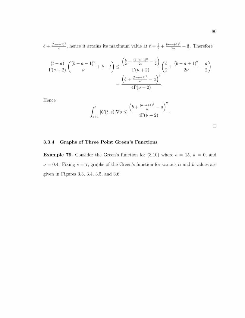
80

b+ (b−a+1)2

ν, hence it attains its maximum value at t = b

2+ (b−a+1)2

2ν+ a

2. Therefore

(t− a)

Γ(ν + 2)

((b− a− 1)2

ν+ b− t

)≤

(b2

+ (b−a+1)2

2ν− a

2

)Γ(ν + 2)

(b

2+

(b− a+ 1)2

2ν− a

2

)

=

(b+ (b−a+1)2

ν− a)2

4Γ(ν + 2).

Hence ∫ b

a+1

|G(t, s)|∇s ≤

(b+ (b−a+1)2

ν− a)2

4Γ(ν + 2).

3.3.4 Graphs of Three Point Green’s Functions


ν = 0.4. Fixing s = 7, graphs of the Green’s function for various α and k values are

given in Figures 3.3, 3.4, 3.5, and 3.6.

81

2 4 6 8 10 12 14t

-2.0

-1.5

-1.0

-0.5

G(t,7)

Figure 3.3: Right Focal Green’s Function as a function of t where b = 15, a = 0,ν = 0.4, α = 0.25, k = 4, and fixed s = 7.

2 4 6 8 10 12 14t

-3.0

-2.5

-2.0

-1.5

-1.0

-0.5

G(t,7)


82

2 4 6 8 10 12 14t

-1.5

-1.0

-0.5

G(t,7)


2 4 6 8 10 12 14t

-2.0

-1.5

-1.0

-0.5

G(t,7)


83

Chapter 4

Applications of the Contraction Mapping Theorem to

Fractional Self-Adjoint Difference Equations

Definition 80 (Contraction Mapping). Let (X, d) be a metric space. Then a map

T : X → X is called a contraction mapping on X if there exists q ∈ [0, 1) such that

d(T (x), T (y)) ≤ qd(x, y) for all x, y in X.

Theorem 81. [24] Let (X, d) be a non-empty complete metric space with a con-

traction mapping T : X → X. Then T admits a unique fixed-point x0 in X (i.e.

T (x0) = x0).

4.1 Long Run Behavior of Equations with Generalized Forcing Terms

Here we will focus on the long run behavior of solutions to the self-adjoint nonlinear

fractional difference equation

∇[p(t)∇νa∗x(t)] = F (t, x(t− 1)), for t ∈ Na+2, (4.1)

where p : Na+1 → (0,∞), 0 < ν < 1, and F : Na+2 × R→ [0,∞).

Remark 82. In a similar methodology of the proof for Theorem 43, we can prove

84

that that the initial value problem

∇[p(t)∇ν

a∗x(t)] = F (t, x(t− 1)), t ∈ Na+2,

x(a) = 0,

∇x(a+ 1) = 0,

has a unique solution. Note that in this section, we specify only one initial condition,

∇x(a + 1) = 0. These results however also specify a boundary condition at infinity,

namely the long run behavior of a solution.

4.1.1 Long Run Behavior Theorem

This subsection’s main result is Theorem 87. In order to prove it, we build up an

equivalence of solutions between the forced fractional difference equation (4.1) and an

integral equation in Theorem 83. Using Theorem 83 and a Lipschitz condition on the

nonlinear forcing term, the Contraction Mapping Theorem is applied in Theorem 87 to

guarantee the existence of a unique solution with long run behavior approaching any

nonnegative real number. See [10] for a similar result in the delta discrete fractional

setting.

Theorem 83. Let p : Na+1 → (0,∞), 0 < ν < 1, and F : Na+2×R→ [0,∞). Define

ζ := x : Na → [0,∞)|x(t) is bounded on Na and ∇x(a + 1) = 0. Furthermore,

assume for all x ∈ ζ,

∫ ∞a

∣∣∣∣∫ k

a

Hν−2(k, ρ(s))

p(s)

∫ s

a+1

F (τ, x(τ − 1))∇τ∇s∣∣∣∣∇k <∞. (4.2)

85

Then, x(t) is a solution to the integral equation

x(t) = L−∫ ∞t

∫ k

a

Hν−2(k, ρ(s))

p(s)

∫ s

a+1

F (τ, x(τ − 1))∇τ∇s∇k, (4.3)

if and only if the forced fractional self-adjoint difference equation

∇[p(t)∇νa∗x(t)] = F (t, x(t− 1)), t ∈ Na+2 (4.4)

has solution x ∈ ζ with limt→∞ x(t) = L.

Before this result is proven, we need two lemmas to simplify the proof. This first

lemma gives us a way to rewrite the integral equation given in Theorem 83.

Lemma 84. Let p : Na+1 → (0,∞), 0 < ν < 1, F : Na+2 × R → [0,∞), and

x : Na → R. Assume (4.2) holds. then

−∫ ∞t

∫ k

a

Hν−2(k, ρ(s))

p(s)

∫ s

a+1

F (τ, x(τ − 1))∇τ∇s∇k

=

∫ t

a

Hν−1(t, ρ(s))

p(s)

∫ s

a+1

F (τ, x(τ − 1))∇τ∇s.(4.5)

Proof. Assume (4.2) and define z(s) := 1p(s)

∫ sa+1

F (τ, x(τ − 1))∇τ . Then consider

∫ ∞t

∫ k

a

Hν−2(k, ρ(s))

p(s)

∫ s

a+1

F (τ, x(τ − 1))∇τ∇s∇k

=

∫ ∞t

∫ k

a

Hν−2(k, ρ(s))z(s)∇s∇k

=∞∑

k=t+1

k∑s=a+1

Hν−2(k, ρ(s))z(s)

=∞∑

k=t+1

t∑s=a+1

Hν−2(k, ρ(s))z(s) +∞∑

k=t+1

k∑s=t+1

Hν−2(k, ρ(s))z(s).

86

Since this summation is absolutely convergent by assumption, we can interchange the

order of summation to get

∞∑k=t+1

t∑s=a+1

Hν−2(k, ρ(s))z(s) +∞∑

k=t+1

k∑s=t+1


=t∑

s=a+1

∞∑k=t+1

Hν−2(k, ρ(s))z(s) +∞∑

s=t+1

∞∑k=s

Hν−2(k, ρ(s))z(s).

Rewriting some of the inner summations in integral form gives

t∑s=a+1

∞∑k=t+1

Hν−2(k, ρ(s))z(s) +∞∑

s=t+1

∞∑k=s


=t∑

s=a+1

∫ ∞t

Hν−2(k, ρ(s))z(s)∇k +∞∑

s=t+1

∫ ∞ρ(s)

Hν−2(k, ρ(s))z(s)∇k.

Evaluating these integrals using Theorem 25 and applying Lemma 26, we get that

t∑s=a+1

∫ ∞t

Hν−2(k, ρ(s))z(s)∇k +∞∑

s=t+1

∫ ∞ρ(s)

Hν−2(k, ρ(s))z(s)∇k

=t∑

s=a+1

(Hν−1(k, ρ(s))z(s)|k→∞k=t

)+

∞∑s=t+1

(Hν−1(k, ρ(s))z(s)|k→∞k=ρ(s)

)=

t∑s=a+1

(0−Hν−1(t, ρ(s))) z(s) +∞∑

s=t+1

(0− 0) z(s)

= −t∑

s=a+1

Hν−1(t, ρ(s))z(s)

= −∫ t

a

Hν−1(t, ρ(s))

p(s)

∫ s

a+1

F (τ, x(τ − 1))∇τ∇s.

87

Therefore

−∫ ∞t

∫ k

a

Hν−2(k, ρ(s))

p(s)

∫ s

a+1

F (τ, x(τ − 1))∇τ∇s∇k

=

∫ t

a

Hν−1(t, ρ(s))

p(s)

∫ s

a+1

F (τ, x(τ − 1))∇τ∇s.

This next lemma helps show that the integral equation in Theorem 83 is nonneg-

ative.

Lemma 85. Let p : Na+1 → (0,∞), 0 < ν < 1, F : Na+2 × R → [0,∞), and

x : Na → R. Then

∫ t

a

Hν−1(t, ρ(s))

p(s)

∫ s

a+1

F (τ, x(τ − 1))∇τ∇s ≥ 0,

for all t ∈ Na.

Proof. Note that by our assumptions on p(t) and F (t, x(t)) being nonnegative, we

have that

1

p(s)

∫ s

a+1

F (τ, x(τ − 1))∇τ ≥ 0, (4.6)

for all s ∈ Na+2. Note for s = a + 1, we have that 1p(s)

∫ sa+1

F (τ, x(τ − 1))∇τ = 0,

hence (4.6) holds for s ∈ Na+1.

Since ν − 1 > −1, we have by Lemma 27 that Hν−1(t, ρ(s)) ≥ 0 for t ∈ Na+1 and

s ∈ Nta+1. Finally, if t = a, we have

∫ taHν−1(t,ρ(s))

p(s)

∫ sa+1

F (τ, x(τ −1))∇τ∇s = 0. Hence

∫ t

a

Hν−1(t, ρ(s))

p(s)

∫ s

a+1

F (τ, x(τ − 1))∇τ∇s ≥ 0,

for all t ∈ Na.

88

Proof of Theorem 83: Assume that x satisfies (4.3) and that (4.2) holds. Then, taking

the nabla difference of (4.3), we get that

∇x(t) =

∫ t

a

Hν−2(t, ρ(s))

p(s)

∫ s

a+1

F (τ, x(τ − 1))∇τ∇s

= ∇1−νa

1

p(t)

∫ t

a+1

F (τ, x(τ − 1))∇τ.

Note here that ∇x(a + 1) = 0. Composing both sides of the previous equation with

the operator ∇−(1−ν)a yields

∇−(1−ν)a ∇x(t) = ∇ν

a∗x(t) =1

p(t)

∫ t

a+1

F (τ, x(τ − 1))∇τ.

Rearranging and taking the nabla difference, we get that

∇ [p(t)∇νa∗x(t)] = F (t, x(t− 1)),

hence x(t) satisfies (4.4).

Since by assumption (4.2) holds, we get that there exists N ∈ Na such that

∣∣∣∣∫ ∞t

∫ k

a

Hν−2(k, ρ(s))

p(s)

∫ s

a+1

F (τ, x(τ − 1))∇τ∇s∇k∣∣∣∣ ≤ 1

for all t ∈ NN . Thus |x(t)| ≤ max|x(a)|, |x(a + 1)|, . . . , |x(N − 1)|, L + 1, hence

x(t) is bounded on Na. Also, by Lemma 84 and Lemma 85 we have that x(t) ≥ 0.

Therefore x ∈ ζ. Finally, since (4.2) holds, limt→∞ x(t) = L. Hence the forward

direction is proven.

Now assume x ∈ ζ where limt→∞ x(t) = L is a solution to (4.4). Then

∇ [p(t)∇νa∗x(t)] = F (t, x(t− 1)).

89

By integrating from a+ 1 to t, we get

p(t)∇νa∗x(t)− p(a+ 1)∇ν

a∗x(a+ 1) =

∫ t

a+1

F (τ, x(τ − 1))∇τ.

By Lemma 37 and since x ∈ ζ, we have that ∇νa∗x(a+ 1) = ∇x(a+ 1) = 0. Hence

p(t)∇νa∗x(t) =

∫ t

a+1

F (τ, x(τ − 1))∇τ.

Rearranging and rewriting yields

∇νa∗x(t) = ∇−(1−ν)

a ∇x(t) =1

p(t)

∫ t

a+1

F (τ, x(τ − 1))∇τ.

Now composing both sides with the operator ∇1−νa gives

∇1−νa ∇−(1−ν)

a ∇x(t) = ∇x(t) = ∇1−νa

1

p(t)

∫ t

a+1

F (τ, x(τ − 1))∇τ

=

∫ t

a

Hν−2(t, ρ(s))

p(s)

∫ s

a+1

F (τ, x(τ − 1))∇τ∇s.

Finally, by integrating from t to infinity, we get that

limb→∞

x(b)− x(t) =

∫ ∞t

∫ k

a

Hν−2(k, ρ(s))

p(s)

∫ s

a+1

F (τ, x(τ − 1))∇τ∇s∇k.

But limb→∞ x(b) = L by assumption, hence

x(t) = L−∫ ∞t

∫ k

a

Hν−2(k, ρ(s))

p(s)

∫ s

a+1

F (τ, x(τ − 1))∇τ∇s∇k,

i.e. x(t) satisfies (4.3).

90

Lemma 86. For 0 < ν < 1 and for any fixed t ∈ Na, we have that

maxs∈Nta+1

|Hν−1(t, ρ(s))| = 1.

Proof. First note that when t = a, we have by convention that Hν−1(t, ρ(s)) = 0 for

s ∈ Na+1, so let t ∈ Na+1 be fixed but arbitrary. Since ν − 1 > −1, we have by

Lemma 27 that Hν−1(t, ρ(s)) ≥ 0. Thus |Hν−1(t, ρ(s))| = Hν−1(t, ρ(s)), for s ∈ Nta+1.

By Lemma 28, we have that ∇sHν−1(t, ρ(s)) ≥ 0. Therefore

maxs∈Nta+1

|Hν−1(t, ρ(s))| = Hν−1(t, ρ(t)) = 1.

Theorem 87. Assume p : Na+1 → (0,∞), 0 < ν < 1, and F : Na+2 × R → [0,∞)

satisfies a Lipschitz condition with respect to its second variable in Na+2 × R, i.e.

there exists M > 0 such that, if u, v ∈ R, then for each fixed t ∈ Na+2,

|F (t, u)− F (t, v)| ≤M |u− v|.

Let ζ := x : Na → [0,∞) : x(t) is bounded on Na, and ∇x(a + 1) = 0 and ‖·‖ be

the supremum norm, noting that (ζ, ‖·‖) is a complete metric space. If

1. the series∑∞

k=a+1

∣∣∣∫ ka Hν−2(k,ρ(s))p(s)

∫ sa+1

F (τ, x(τ − 1))∇τ∇s∣∣∣ converges for all x ∈

ζ, and

2. β := M∫∞a

s−(a+1)p(s)

∇s < 1,

then there exists a unique nonnegative solution of the fractional difference equation

(4.4) with limt→∞ x(t) = L for any L ≥ 0.

91

Proof. Let (ζ, ‖·‖) be the complete metric space noted above, L ≥ 0 be fixed but

arbitrary, and define the operator T as

Tx(t) := L−∫ ∞t

∫ k

a

Hν−2(k, ρ(s))

p(s)

∫ s

a+1

F (τ, x(τ − 1))∇τ∇s∇k.

We want to show that T is a contraction mapping in ζ, so first we show T : ζ → ζ.

Note that in summation notation, Tx is equivalent to

Tx(t) = L−∞∑

k=t+1

∫ k

a

Hν−2(k, ρ(s))

p(s)

∫ s

a+1

F (τ, x(τ − 1))∇τ∇s,

and so by the convergence given in Condition 1, we have that Tx(t) is well defined for

t ∈ Na. Also by the absolute convergence given in Condition 1, there exists N ∈ Na

such that ∣∣∣∣∣∞∑

k=t+1

∫ k

a

Hν−2(k, ρ(s))

p(s)

∫ s

a+1

F (τ, x(τ − 1))∇τ∇s

∣∣∣∣∣ ≤ 1,

for all t ∈ NN . This implies

|Tx(t)| ≤ max|Tx(a)|, |Tx(a+ 1)|, . . . , |Tx(N − 1)|, L+ 1,

for all t ∈ Na, hence Tx is bounded for all t ∈ Na. We also have by Lemma 84 and

Lemma 85 that Tx(t) ≥ 0 for all t ∈ Na. Finally,

∇Tx(t) =

∫ t

a

Hν−2(t, ρ(s))

p(s)

∫ s

a+1

F (τ, x(τ − 1))∇τ∇s,

92

so

∇Tx(a+ 1) =

∫ a+1

a

Hν−2(a+ 1, ρ(s))

p(s)

∫ s

a+1

F (τ, x(τ − 1))∇τ∇s

=a+1∑s=a+1

Hν−2(a+ 1, ρ(s))

p(s)

∫ s

a+1

F (τ, x(τ − 1))∇τ

=Hν−2(a+ 1, a)

p(a+ 1)

∫ a+1

a+1

F (τ, x(τ − 1))∇τ

= 0.

Hence Tx ∈ ζ, thus T : ζ → ζ.

We now show that Tx is contraction mapping. To see this, let x, y ∈ ζ and t ∈ Na

be fixed but arbitrary. By Lemma 84

|Tx(t)− Ty(t)| =∣∣∣∣(L+

∫ t

a

Hν−1(t, ρ(s))

p(s)

∫ s

a+1

F (τ, x(τ − 1))∇τ∇s)

−(L+

∫ t

a

Hν−1(t, ρ(s))

p(s)

∫ s

a+1

F (τ, y(τ − 1))∇τ∇s)∣∣∣∣

=

∣∣∣∣∫ t

a

Hν−1(t, ρ(s))

p(s)

∫ s

a+1

(F (τ, x(τ − 1))− F (τ, y(τ − 1)))∇τ∇s∣∣∣∣

≤∫ t

a

|Hν−1(t, ρ(s))|p(s)

∫ s

a+1

|F (τ, x(τ − 1))− F (τ, y(τ − 1))| ∇τ∇s.

Using the Lipschitz condition assumption, we get that

|Tx(t)− Ty(t)| ≤∫ t

a

|Hν−1(t, ρ(s))|p(s)

∫ s

a+1

M |x(τ − 1)− y(τ − 1)| ∇τ∇s

≤M

∫ t

a

|Hν−1(t, ρ(s))|p(s)

∫ s

a+1

‖x− y‖∇τ∇s

= M ‖x− y‖∫ t

a

|Hν−1(t, ρ(s))|p(s)

(s− (a+ 1))∇s.

93

By Lemma 86,

|Tx(t)− Ty(t)| ≤M ‖x− y‖∫ t

a

1

p(s)(s− (a+ 1))∇s

≤M ‖x− y‖∫ ∞a

s− (a+ 1)

p(s)∇s

< β ‖x− y‖ ,

using Condition 2 to simplify. Since Tx and Ty are bounded and the previous in-

equality is true for all t ∈ Na, we have that

‖Tx− Ty‖ ≤ β ‖x− y‖ ,

but β < 1 by assumption, therefore T is a contraction mapping on ζ. Thus there

exists a unique fixed point x0 ∈ ζ, i.e. x0 = Tx0. This implies

x0(t) = L−∫ ∞t

∫ k

a

Hν−2(k, ρ(s))

p(s)

∫ s

a+1

F (τ, x0(τ − 1))∇τ∇s∇k,

so by Theorem 83, x0(t) solves the forced fractional self-adjoint difference equation

∇ [p(t)∇νa∗x(t)] = F (t, x(t− 1)), t ∈ Na+2,

with limt→∞ x0(t) = L.

4.1.2 Example

Example 88. Let a = 0, ν = 0.6, and p(t) := t3. Let M ∈ R such that 0 < M <

1(π2

6−ζ(3)

) ≈ 2.258, where ζ is the Riemann zeta function. Finally, define F (t, x) :=

M(1 + sin(x)). We will apply the previous theorem. To show that F is uniformly

94

Lipschitz with respect to its second variable, consider the known identity for u, v ∈ R

and fixed t ∈ Na+2

|F (t, u)−F (t, v)| = |(M+M sin(u))−(M+M sin(v))| = M | sin(u)−sin(v)| ≤M |u−v|.

To show the first hypothesis holds, consider

∞∑k=a+1

∣∣∣∣∫ k

a

Hν−2(k, ρ(s))

p(s)

∫ s

a+1

F (τ, x(τ − 1))∇τ∇s∣∣∣∣

=∞∑k=1

∣∣∣∣∫ k

0

H−1.4(k, ρ(s))

s3

∫ s

1

M (1 + sin (x (τ − 1)))∇τ∇s∣∣∣∣

≤∞∑k=1

∫ k

0

∣∣∣∣H−1.4(k, ρ(s))

s3

∣∣∣∣ ∫ s

1

|1 + sin(x(τ − 1))| ∇τ∇s

≤ 2M∞∑k=1

∫ k

0

∣∣∣∣H−1.4(k, ρ(s))(s− 1)

s3

∣∣∣∣∇s= 2M

∞∑k=1

k∑s=1

s− 1

s3|H−1.4(k, ρ(s))| .

Interchanging the summations, we get

2M∞∑k=1

k∑s=1

|H−1.4(k, ρ(s))|s2

= 2M∞∑s=1

s− 1

s3

∞∑k=s

|H−1.4(k, ρ(s))| .

Note H−1.4(k, ρ(s)) = 1 when k = s and H−1.4(k, ρ(s)) ≤ 0 when k ∈ N∞s+1, hence

95

eliminating the absolute value yields

2M∞∑s=1

s− 1

s3

∞∑k=s

|H−1.4(k, ρ(s))| = 2M∞∑s=1

s− 1

s3

[1−

∞∑k=s+1

H−1.4(k, ρ(s))

]

= 2M∞∑s=1

s− 1

s3

[1−

∫ ∞s

H−1.4(k, ρ(s))∇k]

= 2M∞∑s=1

s− 1

s3

[1−

(limb→∞

H−0.4(k, ρ(s))|k=bk=s

)].

By Lemma 26, limb→∞H−0.4(b, s) = 0 for fixed s ∈ N∞1 . Therefore

∞∑k=a+1

∣∣∣∣∫ k

a

Hν−2(k, ρ(s))

p(s)

∫ s

a+1

F (τ, x(τ − 1))∇τ∇s∣∣∣∣ ≤ 4M

∞∑s=1

s− 1

s3<∞,

hence the first hypothesis of Theorem 87 holds.

Finally, we show the second hypothesis holds, i.e. we consider

β := M

∫ ∞a

s− (a+ 1)

p(s)∇s = M

∞∑s=1

s− 1

s3= M

∞∑s=1

s− 1

s3= M

(π2

6− ζ(3)

)< 1.

Thus Theorem 87 applies, so for any fixed L ≥ 0, there exists a unique nonnegative

x(t) that solves the nonlinear self-adjoint difference equation

∇[t3∇0.6

0∗ x(t)]

= M (1 + sin (x (t− 1))) ,

where limt→∞ x(t) = L.

4.2 Unique Solutions to Nonlinear Boundary Value Problems

In this section, we will look at a theorem that uses the Contraction Mapping Theorem

which give sufficient conditions for unique solutions to the specific boundary value

96

problems studied in Chapter 3.

We will consider the nonlinear conjugate boundary value problem

∇∇ν

a∗x(t) = F (t, x(t− 1)), t ∈ Nba+2,

x(a) = A,

x(b) = B,

(4.7)

the nonlinear right-focal boundary value problem

∇∇ν

a∗x(t) = F (t, x(t− 1)), t ∈ Nba+2,

x(a) = A,

∇x(b) = B,

(4.8)

and the nonlinear three point boundary value problem

∇∇ν

a∗x(t) = F (t, x(t− 1)), t ∈ Nba+2,

x(a) = 0,

x(b)− αx(a+ k) = 0,

(4.9)

where 0 < ν < 1, b − a ∈ N2, A,B ∈ R, F : Nba+2 × R → R, 0 ≤ α ≤ 1, and

k ∈ N(b−a)−11 .

4.2.1 Unique Solutions to a Nonlinear Conjugate BVP

We will consider the following nonlinear, self-adjoint, conjugate boundary value prob-

lem given in (4.7)

Theorem 89. Assume F : Nba+2×R→ R satisfies a Lipschitz condition with respect

to its second variable in Nba+2 × R, i.e. there exists a constant K > 0 such that, if

97

u, v ∈ R and t ∈ Nba+2,

|F (t, u)− F (t, v)| ≤ K |u− v| .

If b− a < 2√

Γ(ν+2)√K

, then the nonlinear self-adjoint boundary value problem (4.7) has

a unique solution.

Proof. If x is a solution to (4.7), then it is a solution to the linear self-adjoint boundary

value problem

∇∇ν

a∗x(t) = h(t) := F (t, x(t− 1)), t ∈ Nba+2,

x(a) = A,

x(b) = B.

(4.10)

By Corollary 58, the boundary value problem (4.10) has solution x(t) if and only

if x(t) is a solution to the integral equation

x(t) = w(t) +

∫ b

a+1

G(t, s)h(s)∇s = w(t) +

∫ b

a+1

G(t, s)f(s, x(s− 1))∇s, (4.11)

where w : Nba → R is the unique solution to

∇∇ν

a∗w(t) = 0, t ∈ Nba+2,

w(a) = A,

w(b) = B,

98

and G(t, s) is the Green’s function for

∇∇ν

a∗x(t) = 0, t ∈ Nba+2,

x(a) = 0,

x(b) = 0.

Define ζ := x : Nba → R and ‖x‖ := maxt∈Nba |x(t)|, noting that (ζ, ‖ · ‖) is a

complete metric space. Define the operator T on (ζ, ‖ · ‖) as

Tx(t) := w(t) +

∫ b

a+1

G(t, s)f(s, x(s− 1))∇s,

where w(t) and G(t, s) are given as above. Note that T : ζ → ζ. We claim T is a

contraction mapping, so for a fixed t ∈ Nba, consider for arbitrary x, y ∈ ζ

|Tx(t)− Ty(t)| =∣∣∣∣∫ b

a+1

G(t, s)f(s, x(s− 1))∇s−∫ b

a+1

G(t, s)f(s, y(s− 1))∇s∣∣∣∣

=

∣∣∣∣∫ b

a+1

G(t, s) [f(s, x(s− 1))− f(s, y(s− 1))]∇s∣∣∣∣

≤∫ b

a+1

|G(t, s)||f(s, x(s− 1))− f(s, y(s− 1))|∇s.

Using the Lipschitz condition,

|Tx(t)− Ty(t)| ≤∫ b

a+1

|G(t, s)|K|x(s− 1)− y(s− 1)|∇s

≤ K

∫ b

a+1

|G(t, s)| ‖x− y‖∇s

≤ K ‖x− y‖∫ b

a+1

|G(t, s)|∇s.

99

Then, by the bound on the Green’s function given in Theorem 61, we get

|Tx(t)− Ty(t)| ≤ K ‖x− y‖ (b− a)2

4Γ(ν + 2)= α ‖x− y‖ , (4.12)

where α := K (b−a)2

4Γ(ν+2). Note that this is true for all t ∈ Nb

a, so

‖Tx− Ty‖ ≤ α ‖x− y‖ ,

but, by assumption, b− a < 2√

Γ(ν+2)√K

, so

α <K

4Γ(ν + 2)

(2√

Γ(ν + 2)√K

)2

=K

4Γ(ν + 2)

(4Γ(ν + 2)

K

)= 1,

hence T is a contraction mapping on ζ. So by the Contraction Mapping Theorem,

there exists a unique fixed point x0 ∈ ζ such that

x0(t) = Tx0(t) = w(t) +

∫ b

a+1

G(t, s)f(s, x0(s))∇s,

hence x0(t) is the unique solution to the nonlinear self-adjoint boundary value problem

(4.7).

100

4.2.1.1 Nonlinear Conjugate BVP Example

Example 90. Consider the following boundary value problem.

∇∇0.6

0∗ x(t) = K√x2(t− 1) + 5 + h(t), t ∈ N5

2,

x(0) = A,

x(5) = B,

where K is a constant such that 0 < K < 425

Γ(2.6) ≈ 0.22874 and h : N52 → R.

Note that this is a specific case of (4.7) where a = 0, b = 5, ν = 0.6, and

F (t, x) = K√x2 + 5 +h(t). Then note Fx(t, x) = Kx√

x2+5≤ K for all x ∈ R, hence our

Lipschitz constant for F (t, x) with respect to the second variable is K. But now we

have

2√

Γ(ν + 2)√K

=2√

Γ(0.6 + 2)√K

>2√

Γ(2.6)√425

Γ(2.6)= 5 = b− a.

Hence, by Theorem 89, we have that the above boundary value problem has a unique

solution.

4.2.2 Unique Solutions to a Nonlinear Right Focal BVP


lem given in (4.8)




|F (t, u)− F (t, v)| ≤ K |u− v| .

101

If (b− a)(b− a− 1) < νΓ(2+ν)K

, then the nonlinear self-adjoint boundary value problem

(4.8) has a unique solution.

Proof. The proof will follow nearly identically to Theorem 89. In this case, we have

that w : Nba → R will solve the boundary value problem

∇∇ν

a∗w(t) = 0, t ∈ Nba+2,

w(a) = A,

∇w(b) = B.

In place of (4.12), we would have, as a result of Theorem 65, that

|Tx(t)− Ty(t)| ≤ K ‖x− y‖ (b− a)(b− a− 1)

νΓ(2 + ν)= α ‖x− y‖

where α := K (b−a)(b−a−1)νΓ(2+ν)

. But by assumption (b− a)(b− a− 1) < νΓ(2+ν)K

, so

α := K(b− a)(b− a− 1)

νΓ(2 + ν)< K

νΓ(2 + ν)

KνΓ(2 + ν)= 1,

hence we get T is a contraction mapping on ζ, and the proof finishes in similar manner

to Theorem 89.

4.2.2.1 Nonlinear Right Focal BVP Example


∇∇0.6

0∗ x(t) = K√x2(t− 1) + 5 + h(t), t ∈ N5

2,

x(0) = A,

∇x(5) = B,

102

where K is a constant such that 0 < K < 0.6Γ(2.6)20

≈ 0.04289 and h : N52 → R.

Note that this is a specific case of (4.8) where a = 0, b = 5, ν = 0.6, and




have

νΓ(2 + ν)

K=

0.6Γ(2.6)

K> 5 · 4 = (b− a)(b− a− 1).


solution.

4.2.3 Unique Solutions to a Nonlinear Three-Point BVP


lem given in (4.9)




|F (t, u)− F (t, v)| ≤ K |u− v| .

If (b+ (b−a+1)2

ν−a) <

2√

Γ(ν+2)√K

, then the nonlinear self-adjoint boundary value problem

(4.9) has a unique solution.

Proof. The proof will follow nearly identically to Theorem 89. In this case, we have

that w ≡ 0.

In place of (4.12), we would have, as a result of Theorem 78, that

|Tx(t)− Ty(t)| ≤ K ‖x− y‖(b+ (b−a+1)2

ν− a)2

4Γ(ν + 2)= α ‖x− y‖

103

where α := K(b+

(b−a+1)2

ν−a)2

4Γ(ν+2). But by assumption (b+ (b−a+1)2

ν− a) <

2√

Γ(ν+2)√K

, so

α := K(b+ (b−a+1)2

ν− a)2

4Γ(ν + 2)< K

4Γ(ν + 2)

K4Γ(ν + 2)= 1,

hence we get T is a contraction mapping on ζ, and the proof finishes in similar manner

to Theorem 89.

4.2.3.1 Nonlinear Right Focal BVP Example


∇∇0.6

0∗ x(t) = K√x2(t− 1) + 5 + h(t), t ∈ N5

2,

x(0) = 0,

x(5)− αx(3) = B,

where K is a constant such that 0 < K < 4652

Γ(2.6) ≈ 0.00135, 0 ≤ α ≤ 1, and

h : N52 → R.

Note that this is a specific case of (4.9) where a = 0, k = 3, b = 5, ν = 0.6, and




have

2√

Γ(ν + 2)√K

= 2

√Γ(2.6)√K

> 2

√Γ(2.6)√4

652Γ(2.6)

= 65

=

(5 +

62

0.6− 0

)2

=

(b+

(b− a+ 1)2

ν− a)2

.


solution.

104

Bibliography

[1] Fractional Calculus and Waves in Linear Viscoelasticity. Imperial College Press,

2010.

[2] K. Ahrendt, L. Castle, and K. Yochman. Laplace transforms for the nabla-

difference operator and a fractional variation of parameters formula. Communi-

cations in Applied Analysis, 2011.

[3] K. Ahrendt, L. DeWolf, L. Mazurowski, K. Mitchell, T. Rolling, and D. Ve-

coni. Initial and boundary value problems for the caputo fractional self-adjoint

difference equations. Enlightenment in Pure and Applied Mathematics, 2, 2016.

[4] G.A. Anastassiou. Nabla discrete fractional calculus and nabla inequalities.

Mathematical and Computer Modelling, 2010.

[5] D.R. Anderson. Taylor polynomials for nabla dynamic equations on time scales.

PanAmerican Mathematical Journal, 12, 2002.

[6] George B. Arfken and Hans J. Weber. Mathematical Methods for Physicists.

Academic Press, 6 edition, 2005.

[7] Ferhan M. Atici and Paul W. Eloe. Two-point boundary value problems for finite

fractional difference equations. Journal of Difference Equations and Applications,

17:445–456, 2011.

105

[8] Ferhan M. Atici and Sevgi Sengul. Modeling with fractional difference equations.

J. Math. Anal. Appl., 2010.

[9] F. M. Attici and P. W. Eloe. A transform method in discrete fractional calculus.

International Journal of Difference Equations, 2:165–176, 2007.

[10] Pushp R. Awasthi. Boundary Value Problems for Discrete Fractional Equations.

PhD thesis, University of Nebraska-Lincoln, 2013.

[11] D. Benson, R. Shumer, S. Wheatcraft, and S. Meerschaert. Fractional dispersion,

levy motion, and the made tracer tests. Transport Porous Media, 42:211–240,

2001.

[12] D. Benson, S. Wheatcraft, and M. Meerschaert. Application of a fractional

advection-dispersion equation. Water Resources, 36:1403–1412, 200.

[13] Martin Bohner and Allan Peterson. Dynamic Equations on Time Scales.

Birkhauser, 2001.

[14] Martin Bohner and Allan Peterson. Advances in Dynamic Equations on Time

Scales. Birkhauser, 2003.

[15] A. Brackins. Boundary Value Problems of Nabla Fractional Difference Equations.


[16] Julia St. Goar. A Caputo Boundary Value Problem in Nabla Fractional Calculus.


[17] C. Goodrich and A. C. Peterson. Discrete Fractional Calculus. Springer Inter-

national Publishing, 2015.

106

[18] C. S. Goodrich. Solutions to a discrete right-focal fractional problem. Interna-

tional Journal of Difference Equations, 5:195–216, 2010.

[19] C. S. Goodrich. On a fractional boundary value problem with fractional boundary

conditions. Applied Mathematics Letters, 25:1101–1105, 2012.

[20] Christopher S. Goodrich. An Analysis of Nonlocal Boundary Value Problems of

Fractional and Integer Order. PhD thesis, University of Nebraska-Lincoln, 2012.

[21] J. Hein, S. McCarthy, N. Gaswick, B. McKain, and K. Spear. Laplace transforms

for the nabla difference operator. PanAmerican Mathematical Journal, 21(3):79–

96, 2011.

[22] Michael Holm. Sum and difference compositions in discrete fracctional calculus.

CUBO Mathematical Journal, 13, 2011.

[23] Michael Holm. The theory of discrete fractional calculus: Development and ap-

plication. PhD thesis, University of Nebraska-Lincoln, 2011.

[24] John Hunter and Bruno Nachtergaele. Applied Analysis. World Scientific Pub-

lishing, 2001.

[25] Francesco Mainardi J. A. Tenreiro Machado, Virginia Kriyakova. A poster about

the recent history of fractional calculus. Frtactional Calculus and Applied Anal-

ysis, 13(3), 2010.

[26] W.G. Kelley and A.C. Peterson. The Theory of Differential Equations. Springer,

second edition, 2010.

[27] W.G. Kelley and A.C. Peterson. Difference Equations. Academic Press, second

edition, 2011.

107

[28] S. Hamani M. Benchohra and S. K. Ntouyas. Boundary value problems for

differential equations with fractional order and nonlocal conditions. Nonlinear

Analysis: Theory Methods and Applications, 71:2391–3296, 2009.

[29] S. P. Nasholm and S. Holm. On a fractional zener elastic wave equation. Frac-

tional Calculus and Applied Analysis, 16(1):26–50, 2013.

[30] I. Podlubny. Fractional Differential Equations. Academic Press, 1999.

the existence of solutions for a nonlinear, fractional

Documents