the evaluation of economic forecasts - national bureau of
TRANSCRIPT

This PDF is a selection from an out-of-print volume from the National Bureau of Economic Research
Volume Title: Economic Forecasts and Expectations: Analysis of Forecasting Behavior and Performance
Volume Author/Editor: Jacob A. Mincer, editor
Volume Publisher: NBER
Volume ISBN: 0-870-14202-X
Volume URL: http://www.nber.org/books/minc69-1
Publication Date: 1969
Chapter Title: The Evaluation of Economic Forecasts
Chapter Author: Jacob A. Mincer, Victor Zarnowitz
Chapter URL: http://www.nber.org/chapters/c1214
Chapter pages in book: (p. 3 - 46)

ECONOMIC FORECASTS AND EXPECTATIONS


ONE
The Evaluationof Economic Forecasts
JACOB MINCER AND VICTOR ZARNOWITZ
INTRODUCTION
An economic forecast may be called "scientific" if it is formulated asa verifiable prediction by means of an explicitly stated method whichcan be reproduced and checked.1 Comparisons of such predictions andthe realizations to which they pertain provide tests of the validity andpredictive power of the economic model which produced the forecasts.Such empirical tests are an indispensable basis for further scientificprogress. Conversely, as knowledge accumulates and the models im-prove, the reliability of forecasts, viewed as information about thefuture, is likely to improve.
Forecasts of future economic magnitudes, unaccompanied by anexplicit specification of a forecasting method, are not scientific in theabove sense. The analysis of such forecasts, which we shall call "busi-ness forecasts," is nevertheless of interest.2 There are a number ofreasons for this interest in business forecasts:
NOTE: Numbers in brackets refer to bibliographic references at the end of eachchapter.
'The definition is borrowed from Henri Theil [7, pp. 10 if.].2 In practice, sharp contrasts between scientific economic model forecasts and busi-
ness forecasts are seldom found; more often, the relevant differences are in the degree

4 ECONOMIC FORECASTS AND EXPECTATIONS
1. To the extent that the predictions are accurate, they provide in-formation about the future.
2. Business forecasts are relatively informative if their accuracy isnot inferior to the accuracy of forecasts arrived at scientifically, par-ticularly if the latter are more costly to obtain.
3. Conversely, the margin of inferiority (or superiority) of businessforecasts relative to scientific forecasts serves as a yardstick of prog-ress in the scientific area.
4. Regardless of the predictive performance ascertainable in thefuture, business forecasts represent a sample of the currently prevail-ing climate of opinion. They are, therefore, a datum of some impor-tance in understanding current economic behavior.
5. Even though the methods which produce the forecasts are notspecified by the forecasters, it is possible to gain some understandingof the genesis of forecasts by relating the predictions to other avail-able data.
In this paper we are concerned with the analysis of business fore-casts for some of these purposes. Specifically, we are interested inmethods of assessing the degree of accuracy of business forecasts bothin an absolute and in a relative sense. In the Absolute Accuracy Analy-sis (Section I) we measure the closeness with which predictions ap-proximate their realizations. In the Relative Accuracy Analysis (Sec-tion II) we assess the net contributions, if any, of business forecaststo the information about the future available from alternative, relativelyquick and cheap methods. The particular alternative or benchmarkmethod singled out here for analysis is extrapolation of the pasthistory of the series which is being predicted. The motivation for thischoice of benchmark is spelled out in Section II. It will be apparent,however, that our relative accuracy analysis is suitable for compari-Sons of any two forecast methods.
The treatment of extrapolations as benchmarks against which thepredictive power of business forecasts is measured does not imply
to which the predictions are explicit about their methods, and are reproducible. In-formation on the methods is not wholly lacking for the business forecasts, nor is it al-ways fully specified for econometric model predictions. Note also that distinctions be-tween unconditional and conditional forecasting, or between point and interval forecastsare not the same as between scientific and nonscientific forecasts. The latter are usuallyunconditional point predictions, but so can "scientific" forecasts be. [Cf. 7. p. 4.]

EVALUATION OF FORECASTS S
that business forecasts and extrapolations constitute mutually exclu-sive methods of prediction. It is rather plausible to assume that mostforecasts rely to some degree on extrapolation. If so, forecast errorsare partly due to extrapolation errors. Hence, an analysis of the pre-dictive performance of extrapolations can contribute to the understand-ing and assessment of the quality of business forecasts. Accordingly,we proceed in Section III to inquire into the relative importance ofextrapolations in generating business forecasts, and to study the ef-fects of extrapolation error on forecasting error.3
All analysts of economic forecasting owe a large intellectual debt toHenri Theil, who pioneered in the field of forecast evaluation. A partof the Absolute Accuracy Analysis section in this paper is an expan-sion and direct extension of Theil's ideas formulated in [8]. Our treat-ment, indeed, parallels some of the further developments which Theilrecently published.4 However, while the starting point is similar, weare led in different directions, partly by the nature of our empiricalmaterials, and partly by a different emphasis in the conceptual frame-work. The novel elements include our treatment of explicit benchmarkschemes for forecast evaluation, which goes beyond the familiar naivemodels to autoregressive methods; our attempt to distinguish theextrapolative and the autonomous components of the forecasts; andour analysis of multiperiod or variable-span forecasts and extrapola-tions.
The empirical materials used in this paper consist of eight differentsets of business forecasts, denoted by eight capital letters, A throughH. These forecasts are produced by groups of business economists,economic departments of large corporations, banks, and financialmagazines. Most use is made here, for illustrative purposes, of a sub-group of three sets of forecasts, E, F, and G, which represent a largeopinion poii and small teams of business analysts and financial experts.The data for all eight sets summarize the records of several hundredforecasts, all of which have been prc,cessed in the NBER study ofshort-term economic forecasting.5 It is worth noting that our substan-tive conclusions in this paper are broadly consistent with the evidence
' For an analysis of a particular extrapolation method, known as "adaptive forecast-ing," see Jacob Mincer, "Models of Adaptive Forecasting," Chapter 3 in this volume.
Theil [7, Chapter 2, especially pp. 3 3—36].For a detailed description of data and of findings, see [13].

6 ECONOMIC FORECASTS AND EXPECTATIONS
based on the complete record. A summary of the analyses and of thefindings is appended for the benefit of the impatient reader.
I. ABSOLUTE ACCURACY ANALYSIS
ERRORS IN PREDICTIONS OF LEVELS
At the outset, it will be helpful to state a few notations and defini-tions: represents the magnitude of the realization at time (t + A-);and z÷kPs, the prediction of At÷k at time t. The left-hand subscript of Pis the target date, the right-hand subscript is the base date of the fore-cast; and k is the time interval between forecast and realization, alsocalled the forecast' span.
Although the terms "forecast" and "prediction" are synonyms ingeneral usage, we shall reserve the former to describe a set of predic-tions produced by a given forecaster or forecasting method, and per-taining to the set of realizations of a given time series A. Singlepredictions t+kPt are elements in the set, or in the forecast P, just assingle realizations A(+k are elements in the time series A. Differentforecasts (methods or forecasters) may apply to the same set ofrealizations, but not conversely.6
Consider a population of constant-span (say, k = 1) predictions andrealizations of a time series A. The analytical problem is to devisecomparisons between forecasts ,P1_1 and realizations which willyield useful descriptions of sizes and characteristics of forecastingerrors = —
A simple and useful graphic comparison is obtained in a scatterdiagram relating predictions to realizations.7 As Figure 1 indicates,a perfect prediction = 0) is represented by a point on the 450 linethrough the origin, the line of perfect forecasts (LPF). Clearly, thesmaller the dispersion around LPF the more accurate is the forecast.A measure of dispersion around LPF can, therefore, serve as a meas-ure of forecast accuracy. One such measure, the variance around LPF,is known as the mean square error of forecast. We will denote it by
For some purposes, not considered in this paper, the converse may be admissible.A forecaster may be evaluated by the performance of a number of forecasts he pro-duced, each set of predictions pertaining to different sets of realizations.
The "prediction-realization diagram" was first introduced by Theil in [8, pp. 30 if.].

EVALUATION OF FORECASTS 7
Its definition is:
(1) = E(A — P)2,
where E denotes expected value. Preference for this measure as ameasure of forecast accuracy is based on the same considerationsas the preference for the variance as a measure of dispersion inconventional statistical analysis: This is its mathematical and statisti-cal tractability. We note, of course, that this measure gives more than
FIGURE 1-1. The Prediction-Realization Diagram
— Line of perfect forecasts— Regression line— Mean realization— Mean prediction— Mean corrected prediction— Mean point— Corrected mean point
RealizationsA
P
Key:L PFRLAPbc
E

8 ECONOMIC FORECASTS AND EXPECTATIONS
proportionate weight to large errors, an assumption which is not par-ticularly inappropriate in economic forecasting.8
The square root of measures the average size of forecast error,expressed in the same units as the realizations. The expression = 0
represents the unattainable case of perfection, when all points in theprediction-realization diagram lie on LPF. In general, most points areoff LPF. However, special interest attaches to the location of themean point, defined by [E(A), E(P)]. The forecast is unbiased if thatpoint lies on LPF, that is if E(P) = E(A). The difference E(A) — E(P) =E(u) measures the size of bias. The forecast systematically under-estimates or overestimates levels of realizations, if the sign of the biasis positive or negative, respectively.
Unbiasedness is a desirable characteristic of forecasting, but it doesnot, by itself, imply anything about forecast accuracy. Biased fore-casts may have a smaller than unbiased ones. However, otherthings being equal, the smaller the bias, the greater the accuracy of theforecast. The "other things" are the distances between the points ofthe scatter diagram: Given that E(P) E(A), a translation of the axesto a position where the new LPF passes through the mean point willproduce a mean square error, which is smaller than the originalThis is because the variance around the mean is smaller than the vari-ance around any other value.
Formally, we have:
(2) = E(A — P)2 = E(u2) = [E(u)]2 + cr2(u)
and
= o2(u).
The presence of bias augments the mean square error by the meancomponent [E(u)]2. The other component of the variance of theerror around its mean, o-2(u), is an (inverse) measure of forecastingefficiency.
Further consideration of the prediction-realization scatter diagramyields additional insights into characteristics of forecast errors. Thusnonlinearity of the scatter indicates different (on average) degrees of
'From a decision point of view, this measure is optimal under a quadratic loss cri-terion. For an extensive treatment of this criterion see Theil [9].

EVALUATION OF FORECASTS 9
over- or underprediction at different ranges of values. its heteroscedas-ticity reflects differential accuracy at different ranges of values.
These properties of the scatter are difficult to ascertain in smallsamples. Of greater interest, therefore, is the inspection of a least-squares straight-line fit to the scatter diagram. The mean point is onepoint on the least-squares regression line. Just as it is desirable for themean point to lie on the line of perfect forecasts, so it would seem in-tuitively to be as desirable for all other points. In other words, thewhole regression line should coincide with LPF. If the forecast isunbiased, but the regression line does not coincide with LPF, it mustintersect it at the mean point. At ranges below the mean, realizationsare, on average, under- or overpredicted, with the opposite tendencyabove the mean. The greater the divergence of the regression line fromLPF, the stronger this type of error. In other words, the larger thedeviation of the regression slope from unity, the less efficient the fore-cast: It is intuitively clear that rotation of the axes until LPF coincideswith the regression line will reduce the size of cr2(u).
Before the argument is expressed rigorously, one matter must bedecided: As is well known, two different regression lines can be fitted inthe same scatter, depending on which variable is treated as predictorand which is predictand. Because, by definition, the forecasts are pre-dictors, and because they are available before the realizations, wechoose P as the independent and A as the dependent variable.
While
(3)
is an identity, a least-squares regression of on produces, generally:
(4)
Only when the forecast error is uncorrelated with the forecast valuesis the regression slope f3 equal to unity, in this case, the residual
variance in the regression o2(v) is equal to the variance of the forecasterror cr2(u). Otherwise, cT2(u) > o'2(v). Henceforth, we call forecastsefficient when o'2(u) = o-2(v). If the forecast is also unbiased, 0,cr2(v) = cr2(u) =
To illustrate the argument, consider a forecaster who underestimatedthe level of the predicted variable repeatedly over a succession oftime periods. His forecasts would have been more accurate if they were

10 ECONOMIC FORECASTS AND EXPECTATIONS
all raised by some constant amount, i.e., the historically observedaverage error. Other things being equal—specifically, assuming thatthe process generating the predicted series remains basically un-changed as does the forecasting method used—such an adjustmentwould also reduce the error of the forecaster's future predictions. Nowsuppose that the forecaster generally underestimates high values andoverestimates low values of the series, so that his forecasts can besaid to be inefficient. Under analogous assumptions, he could reducethis type of error by raising his forecasts of high values and loweringthose of low values by appropriate amounts.
Since, generally, o-2(u) o-2(v), a forecast which is unbiasedand efficient is desirable. In the general case of biased and/or inefficientforecasts, we can think of regression (4) as a method of correcting theforecast to improve its accuracy.9
The corrected forecast is PC a + and the resulting mean squareerror equals M$ = o2(u) M,. We can visualize this linearcorrection as being achieved in two steps: (I) A parallel shift of theregression line to the right until the mean point is on the 450 diagonalin Figure 1. This eliminates the bias and reduces the mean squareerror to o-2(u), in equation 2. (2) A rotation of the regression linearound the mean point (E = EC) until it coincides with LPF (i.e.,/3 = 1). This further reduces the to 472(v).
We can express the successive reductions as components of themean square error:
(5) = E(u)2 = {E(u)]2 + ff2(u) = [E(u)]2 + [o.2(u) — + cr2(v).
"Theil calls it the "optimal linear correction," [7, p. 33, ff.1.It might be tempting to call optimal those forecasts which are both unbiased and
efficient. We refrain from this terminology for the following reason: The regressionmodel (4), in which we regress A on P rather than conversely, can also be interpretedby viewing realizations (A,) as consisting of a stochastic component €, and a nonstochas-tic part A, [cf. 7, Ch. 2], (4a) A, = A, + €,, with E(e,) = 0, and E(A,€,) = 0.
The stochastic component can be viewed as a "random shock" representing theoutcome of forces which make future events ultimately unpredictable. The forecasterdoes his best trying to predict A, attaining €, as the smallest, irreducible forecast error.Thus, we prefer to reserve the notion of optimality to forecasts P, = A, whose isminimal, namely = o.2(€,). It is clear, from this formulation, that optimal forecasts areunbiased and efficient, but the converse need not be true. Questions of optimality arenot directly considered in the present study.
The concept of "rational forecasting," as defined by J. F. Muth [5, pp. 3 15—335],implies unbiased and efficient forecasts utilizing all available information.

EVALUATION OF FORECASTS 11
If denotes the coefficient of determination in the regression of Aon P, then r2(v) = (1 — Also,'° cr2(u) — cr2(v) = (1 — /3)2o2(P).
Hence, the decomposition of the mean square error is:
(5a) = [E(u)]2 + (1 — /3)2o-2(P) + (1 —
We call the first component on the right the mean component (MC),the second the slope component (SC), and the third the residual com-ponent (RC) of the mean square error. In the unbiased case, MCvanishes; in the efficient case SC vanishes. In forecasts which areboth unbiased and efficient both MC and SC vanish, and the meansquare error equals the residual variance (RC) in (4).
Thus far we have analyzed the relation between predictions andrealizations in terms of population parameters. However, in empiri-cal analyses we deal with limited samples of predictions and realiza-tions. The calculated mean square errors, their components, and theregression statistics of (4) are all subject to sampling variation. Thus,even if the predictions are unbiased and efficient in the population, thesample results will show unequal means of predictions and realiza-tions, a nonzero intercept in the regression of A on P, a slope of thatregression different from unity, and nonzero mean and slope compo-nents of the mean square error. To ascertain whether the forecasts areunbiased and/or efficient, tests of sampling significance are required.
Expressing the statistics for a sample of predictions and realizations,regression (4) becomes:(6)
and, corresponding to (5a), the decomposition of the sample meansquare error, is:
(7)
The test that P is both unbiased and efficient is the test of the jointnull hypothesis a = 0 and /3 = 1 in (4). If the joint hypothesis is re-jected, separate tests for bias and efficiency are indicated. The respec-tive null hypotheses are E(u) 0 and /3 = 1.
= ff2(A) + cr2(P) — 2 Coy (A, P) = o-2(A) + —
cr2(v) = o-2(A) —
Subtracting, o2(u) — = o-2(P) — 213cr2(P) + = (1 — /3)2a2(P)

12 ECONOMIC FORECASTS AND EXPECTATIONS
TABLE 1-1. Accuracy Statistics for Selected Forecasts of Annual Levels of FourAggregative Variables, 1953—63
Code and
A. Summary Statistics for Predictions (P), Realizations (A), and Errors
Root Percentage of Accounted for byStandard Mean
Mean Deviation Square Mean Slope ResidualType of Error Component Component Variance
Line Forecast a Ab P SA VM (MC) (SC) (RV)(1) (2) (3) (4) (5) (6) (7) (8)
Gross National Product (GNP)(billion dollars)
1 E (11) 458.1 447.3 76.4 79.3 16.7 39.4 5.4 55.22 F (11) 458.1 453.2 76.4 79.5 8.8 28.1 14.0 57.93 G (11) 458.1 459.9 76.4 82.3 7.9 4.6 54.8 40.6
Personal Consumption Expenditures (PC)(billion dollars)
4 E (11) 296.4 287.6 49.0 52.6 5.5 76.2 12.2 11.75 F (11) 296.4 293.4 49.0 52.1 10.0 27.7 27.8 44.5
Plant and Equipment Outlays (PE)(billion dollars)
6 E (10) 32.6 32.0 3.8 5.2 2.9 4.2 44.1 51.7
Index of Industrial Production (IP)(index points, 1947—49 = 100)
7 E (Ii) 149.6 148.8 21.6 21.9 6.0 1.7 3.1 95.18 F (11) 149.6 150.4 21.6 21.8 4.6 2.6 2.0 95.49 0 (11) 149.6 152.1 21.6 23.3 4.8 24.2 17.0 58.7
(continued)
Table 1-1 presents accuracy statistics for several sets of businessforecasts of GNP, consumption, plant and equipment outlays, andindustrial production. Part A shows means and variances of predic-tions and realizations, as well as the mean square error and its com-ponents expressed as proportions of the total. Part B shows the re-gression and test statistics for the hypotheses of unbiasedness andefficiency.
The statistical tests in most cases reject the joint hypothesis of un-biasedness and efficiency. This is accounted for largely by bias, andthe preponderant bias is an underestimation of consumption and of

EVALUATION OF FORECASTS 13
TABLE 1-1 (concluded)
Line
Code andType of
Forecast a
B. Regression and Test Statistics
F-Ratio for(a = 0,
a b /3 = 1)
(1) (2) (3) (4)
t-Test forE(A) = E(P)
(5)
t-Test for/3 =
(6)
Gross National Product (GNP)101112
E (11)F (11)G (11)
33.252 .950 .972 3.85 *24.357 .957 .992 2.4532.531 .925 .995 *
—2.68 *—2.07 *
•931.47 **349 *
Personal Consumption Expenditures (PC)1314
E (11).F (11)
28.753 .931 .995 40.04*20.893 .939 .994 68.20 * —2.07 *
3.25*2.61 *
Plant and Equipment Outlays (PE)15 £ (10) 13.256 .605 .667 3.70* —.66 2.61*
Index of Industrial Production (IP)161718
E (11)F (11)G (11)
8.771 .950 .918 .143.968 .968 .952 .24
10.989 .912 .968 3.10*
—.44.54
1.87*
.53
.431.62**
Number of years covered is given in brackets. All forecasts refer to the period 195 3—63, except theplant and equipment forecasts E (line 6), which cover the years 1953—62.
The realizations (A) are the first annual estimates of the given variable reported by the compiling agency.* Significant at the 10 per cent level.• * Significant at the 25 per cent level.
GNP. Most of the forecasts seem inefficient. However, the degree ofinefficiency is relatively minor, as the regression slopes are close tounity, though they are consistently below unity (Part B, column 2).
The decomposition of the mean square error in Part A of Table 1-1suggests that the residual variance component is by far the most im-portant component of error, and the slope component rather negli-gible. The mean component often accounts for as much as one-fourthof the total mean square error.
The correlations between forecasts and realizations are all positiveand very high (their squares are shown in Part B, column 3). This isto be expected in series dominated by strong trends. Where trend dom-

14 ECONOMIC FORECASTS AND EXPECTATIONS
ination is weaker, as in the plant and equipment series, the correlationis lower. These coefficients do not measures or componentsof absolute forecasting accuracy. They are shown here merely for thesake of completeness and conventional usage. The coefficient of deter-mination is, at best, a possible measure of relative accuracy. It spe-cifically relates the mean square error of a linearly corrected forecastto the variance of realization [see Section III, equation (18), note 28].This is not a generally useful measure of forecasting accuracy.
ERRORS IN PREDICTIONS OF CHANGES
Economic forecasts may be intended and expressed as predictions.of changes rather than of future levels. The accuracy analysis of levelscan also be applied to comparisons of predicted changes (P, — A,...,)with realized changes (A, —A,_,). A complicating factor in this analysisof changes are base errors, due to the fact that the value of A,_, wasnot fully known at the time the forecast was made.'1 This is why thebase is denoted by A,_,.
If the forecast base were measured without error, the accuracystatistics for changes would be almost identical with those for levels.Clearly, the forecast error and, hence, the mean square error wouldbe the same since:
(A, — A,_,) — (F, — A,_,) = A, — P1 = Ut.
By the same token, the mean and variance components of the meansquare error would be identical. The only difference would emerge inthe decomposition of the variance into slope and residual components.This is because the regression of on (P,—A,_,) differs fromthe regression of A, on P,.
Denote the regression slope in this case by
Coy (A, —A,_,, P,2 '
from which it follows that:
Though we excluded them in the preceding section, base errors also tend to obscuresomewhat the analysis of forecast errors in predictions of levels. For an intensiveanalysis of the effects of base errors on forecasting accuracy, see Rosanne Cole, "DataErrors and Forecasting Accuracy," in this volume.

EVALUATION OF FORECASTS 15
— Coy (u,, — Coy (ui, F,)(8) 1 —
— cr2(P, — A,_1)
Assume that the level forecast is efficient in the sense that f3 = 1,
because Coy (u,, F,) = 0. Then = 1 only if Coy (u,, A,...,) = 0. Theadditional requirement that Coy (U,, A,_,) = 0 for the efficiency of fore-casts of changes 12 is an additional aspect of efficiency in forecasts oflevels. It indicates that forecast errors cannot be reduced by takingaccount of past values of realizations or, put in other words, the extrap-olative value of the base (A,_,) has already been incorporated in theforecast.
In Table 1-2 the same accuracy statistics are shown for forecasts ofchanges as were shown for forecasts of levels in Table 1-1. We notethat, while the regression slopes b in Table 1-1 were close to unity,here they are substantially smaller. It appears that this is explainablelargely by a positive Coy (u,, A,...,) in equation (8) and also as an effectof base errors.'3 Not surprisingly, the correlations between forecastsand realization (Part B, column 3) are weaker here than they are forpredictions of levels.
UNDERESTIMATION OF CHANCES
A systematic and repeatedly observed property of forecasts is thetendency to underestimate changes. Comparisons of predicted andobserved changes permit the detection of such tendencies. We searchfor their presence also in our data.
In order to understand better the empirical results, it is useful todefine clearly the existence of such tendencies and to inquire into theirpossible sources.'4 Underestimation of change takes place wheneverthe predicted change (F, — A,...,) is of the same sign but of smaller size
12 = I also when Coy (U,, A,_,) = Coy (ui, P,) 0. However, in that case both leveland change forecasts are inefficient, since is larger when Coy (u,, P,) 0 than whenit is zero.
" See Rosanne Cole's essay, pp. 64—70 of this volume. It might seem that the baseerrors which bias the regression slopes downward in Table 1-2 would also increase themean square errors of predicted changes compared to the mean square error in levels.This is not necessarily true, however, and Table 1-2, in fact, shows mean square errorssmaller than in Table 1-1. According to Rosanne Cole's analysis, the explanation, again,lies in the way base errors affect forecasts.
For a different and more extensive discussion of this issue, see Theil [8, especiallyChapter V].
16 ECONOMIC FORECASTS AND EXPECTATIONS
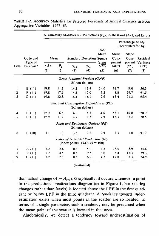
TABLE 1-2. Accuracy Statistics for Selected Forecasts of Annual Changes in FourAggregative Variables, 1953—63
A. Summary Statistics for Predictions (Pa), Realizations and Errors
Percentage ofAccounted for by
RootMean Mean Slope
Code and Mean Standard Deviation Square Corn- Corn- ResidualType of Error ponent ponent Variance
Line Forecast a b (MC) (SC) (R V)(1) (2) (3) (4) (5) (6) (7) (8)
Gross National Product (GNP)(billion dollars)
1 E (11) 19.8 11.3 14.1 13.4 14.0 34.7 9.0 56.32 F (11) 19.8 17.5 14.1 17.0 7.5 8.8 29.7 61.53 G (11) 19.8 22.8 14.1 16.2 7.9 13.4 21.2 65.4
Personal Consumption Expenditures (PC)(billion dollars)
4 E (11) 12.9 6.5 4.9 6.5 4.6 63.1 16.0 20.95 F (11) 12.9 11.2 4.9 8.3 7.9 12.3 67.2 20.5
Plant and Equipment Outlays (PE)(billion dollars)
6 E (10) 1.1 .3 3.5 2.2 2.9 7.3 1.0 91.7
Index of Industrial Production (IP)(index points, 1947—49 = 100)
7 E (11) 5.2 2.4 8.6 5.0 6.3 18.5 5.9 75.68 F (11) 5.2 4.5 8.6 9.5 3.6 3.4 17.3 79.39 G (11) 5.2 7.1 8.6 8.9 4.3 17.8 7.3 74.9
(continued)
than actual change Graphically, it occurs whenever a pointin the predictions — realizations diagram (as in Figure 1, but relatingchanges rather than levels) is located above the LPF in the first quad-rant or below LPF in the third quadrant. A tendency toward under-estimation exists when most points in the scatter are so located. Interms of a single parameter, such a tendency may be presumed whenthe mean point of the scatter is located in that area.
Algebraically, we detect a tendency toward underestimation of
EVALUATION OF FORECASTS 17
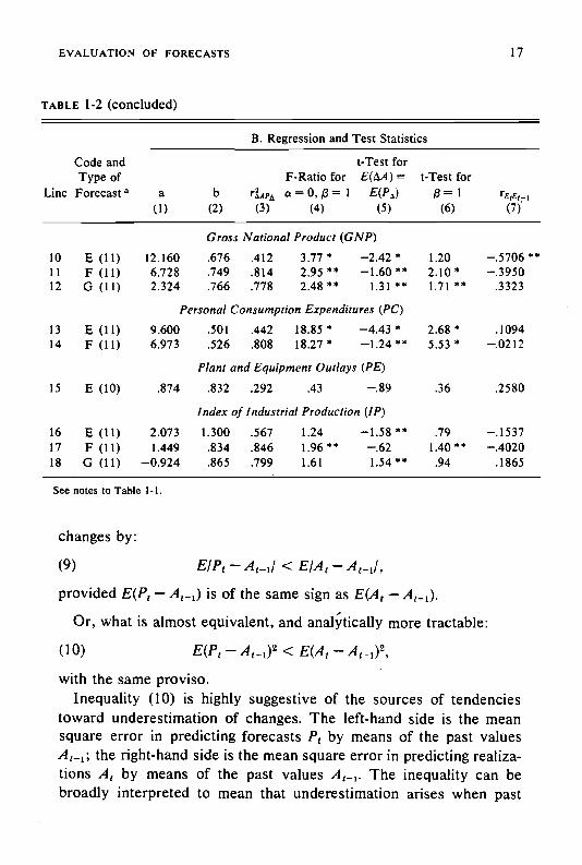
TABLE 1-2 (concluded)
Line
Code andType ofForecast
B. Regression and Test Statistics
t-Test forF-Ratio for =
a b rLpA a = 0, $ 1
(1) (2) (3) (4) (5)
t-Test for/3 = 1
(6)r515,_1
(7)
Gross National Product (GNP)101112
E (11)F (11)G (11)
12.160 .676 .412 377*6.728 .749 .814 2.95**2.324 .766 .778 2.48** 1.31 **
1.202.10*1.71 **
—.3950.3323
Personal Consumption Expenditures (PC)1314
E (11)F (11)
9.600 .501 .442 18.85*6.973 .526 .808 18.27*
2.68*553*
.1094—.0212
Plant and Equipment Outlays (PE)15 E (10) .874 .832 .292 .43 —.89 .36 .2580
Index of Industrial Production (IP)16
17
18
E (11)
F (11)
0 (11)
2.073 1.300 .567 1.24
1.449 .834 .846 1.96** —.62
—0.924 .865 .799 1.61 1.54**
.791.40**.94
—.1537—.4020.1865
See notes to Table 1-1.
changes by:
(9) — <E/A1 —
provided — A1_1) is of the same sign as E(A1 —
Or, what is almost equivalent, and more tractable:
(10) — < —
with the same proviso.Inequality (10) is highly suggestive of the sources of tendencies
toward underestimation of changes. The left-hand side is the meansquare error in predicting forecasts by means of the past values
the right-hand side is the mean square error in predicting realiza-tions by means of the past values The inequality can bebroadly interpreted to mean that underestimation arises when past

18 ECONOMIC FORECASTS AND EXPECTATIONS
events bear a closer (and positive) relation to the formation of fore-casts than to future realizations. This is very plausible. Forecastsdiffer from realizations because information is incomplete. To theextent that some elements of information are lacking, the effect islikely to be produced.
Now, decomposing (10), we get:
(11)— + — A1_1) < [E(A,) — +
According to (II), underestimation of changes occurs because:(12a) E(P1)
when both and are greater than A1_1, or
(12b) E(P1) >
when both and are less than and/or because
(13) — < — A1_1).
It is important to note that condition (13) necessarily holds when pre-dictions of changes are efficient, i.e., when = 1, because, in thatcase: o2(A1 — = + cT2(Ut).15 Thus, underestimation ofchanges is a property of unbiased and efficient forecasts of changes,or, what is equivalent, of unbiased and efficient forecasts of levels inwhich all of the extrapolative information contained in the base (A1_1)has been exploited.t6 But, as the analysis shows, it can also arise inbiased or incorrect forecasting.
In Table 1-2, the actual forecast base contains errors. These,as we noted, tend to bias the regression slopes downward. They maytherefore contribute to the observed reversal of inequality (13). Ascomparisons of columns 3 and 4, Part A, show, > S2(A,—
A1_1) in six of the nine recorded cases. Whether a better agreementwith the inequality in (13) would obtain in the absence of base errors
Since A, — A, = P, — A,_ + u,, it follows that var (A, — A,_1) = var (P, — A,_) +var (u,) + 2 coy (P, — A,.,, u,). But the last term in the above vanishes under the assumedconditions, since, for efficient forecasts with = I, coy (u,_,, A,_,) = coy (U,, P,) = 0(see note 12).
' A fortiori, underestimation of changes is a property of "rational" forecasting in thesense of Muth [5, p. 334].

EVALUATION OF FORECASTS 19
is not clear. It depends,. in part, on the effects past errors exert on theforecast levels
Where the variance of predicted change exceeds the variance ofactual change in Table 1-2, the source of underestimation of changesin our data must lie in the underestimation of levels (12). This char-acteristic is observed in Table 1-1. Changes are, indeed, underesti-mated in all these forecasts where levels were underestimated, andoverestimated in those few forecasts where levels were overestimated.(Compare Part A, columns I and 2,-of Tables 1-1 and 1-2.)
The tendency to underestimate changes is explored in greater detailin Table 1-3. Here each of the individual predictions of change isclassified as an under- or overestimate. We find that two-thirds of theincreases in GNP were underestimated, and one-third overestimated.But of the decreases, which were relatively few and shallow, half weremissed and barely one-fourth underestimated. For consumption, noyear-to-year decreases are recorded, and underpredictions of in-creases represent nearly two-thirds of all observations. It seems un-likely that such high proportions could be due to chance.
At the same time, in series with weaker growth but stronger cyclicaland irregular movements, underestimates of increases, while frequent,are not dominant. Table 1-3 shows this clearly for the forecasts ofgross private domestic investment and plant and equipment outlays.For industrial production, the situation is similar, though the pro-portion of underestimates for the decreases may be significant.'8
We conclude that the underestimation of changes reflects mainly aconservative prediction of growth rates in series with upward trends.This implies, in turn, that the levels of such series must also be under-estimated, a fact already noted. To what extent the purported general-ity of underestimation of changes is true beyond the conservative un-derestimation of increases remains an open question.
'7The reader is referred again to Rosanne Cole's essay. Here we may note thatto the extent that base errors are incorporated in P,. S2(P,) is augmented. This mayexplain the observation in Table I - I where > S2(A,) in all cases (columns 3 and4. Part A).
18 It should be noted that Table 1-3 includes all forecast sets that have thus far beenanalyzed in the NBER study and is thus based on much broader evidence than TableI-I. In particular, the representation of investment forecasts is greatly strengthenedhere by the inclusion of gross private domestic investment forecasts (GNP component)along with those of plant and equipment outlays (OBE-SEC definition).

20 ECONOMIC FORECASTS AND EXPECTATIONS
TABLE 1-3. Forecasts of Annual Changes in Five Comprehensive Series, Distribu-tion by Type of Error, 1953—63
Predicted Variable
Forecast of An nual Changes b Probabilityof as Many
or MoreTurningand Total Under- Over- Point Under-
Type of Change a Number(1)
estimates(2)
estimates(3)
Errors(4)
estimates(5)
Gross national product (8)Increases 64 43 21 0 .004Decreases 14 3 4 7 .756
Personal consumption expenditure (5)Increasesd 45 29 13 3 .010
Gross private domestic investment (4)Increases 22 10 9 3 .500Decreases 12 5 4 3 .500
Plant and equipment outlays (2)Increases 5 4 2 .500Decreases 5 2 3 0 .812
industrial production (7)Increases 57 28 23 6 .288Decreases 13 9 3 1 .073
0 The number of forecast sets covered is given in parentheses. Increases and decreases refer to the direc-tion of changes in the actual values (first estimates for the given series).
Underestimates indicate that predicted change is less than the actual change; overestimates, that pre-dicted change exceeds actual change; turning point errors, that the sign of the predicted change differs fromthe sign of the actual change.
Based on the proportion of all observations, other than those with turning point errors, accounted forby the underestimates (i.e., column 2 divided by the difference between column I and column 4). Prob-abilities taken from Harvard Computation Laboratory, Tests of the Cumulative Binomial Probability Dis-tribution, Cambridge, Mass., 1955.
All observed changes are increases.° Includes one perfect forecast (hence the total of observations in columns 2—4 in this line is II).
II. RELATIVE ACCURACY ANALYSIS
The quality of forecasting performance is not fully described by thesize and characteristics of forecasting error as analyzed in Section 1.Sizes of forecasting errors cannot even be compared when sets of pre-dictions differ in target dates or in the economic variables to be pre-dicted. Theil goes beyond the matter of comparability in suggestingthat a sharp distinction must be made between size of forecasting error

EVALUATION OF FORECASTS 21
and consequences of forecasting error. According to him, "the qualityof a forecast is determined by the quality of the decision to which itleads." 19
This emphasis on consequences can be further generalized by re-lating, incrementally, the gains obtainable from reducing forecasterrors which the particular forecasting method accomplishes relativeto an alternative, to the cost of producing such reductions. In prin-ciple, such a rate-of-return criterion is a ratio of imputed dollar val-ues, in which numerator and denominator provide for comparabilityand for an economically unambiguous ranking of forecasting perform-ance regardless of target dates and variables.
In this part of our analysis, we suggest a criterion for the appraisalof forecasting quality which derives from this economic concept butis necessarily more limited. In the absence of a gain function (for thenumerator) and of an investment cost function (for the denominator),we measure the payoff only in terms of the reduction in forecastingerror obtained by the forecast (P) compared with an alternative, lesscostly, "benchmark" method (B). The benchmark we propose is theextrapolation of the past own history of the target series. Our pro-posed index of forecasting quality is the ratio of the mean square errorof forecast to the mean square error of extrapolation M1. The ratiorepresents the relative reduction in forecasting error. It ranks thequality of forecasting performance the same way as a rate-of-returnindex, in which the return (numerator) is inversely proportional tothe mean square error of forecast, and the cost (denominator) inversely
20 to the mean square error of extrapolation, the latterrepresenting the difficulties encountered in forecasting a given series.
Benchmarks other than extrapolations could be used when the com-parison is considered relevant. In this sense, our procedure is generaland the particular benchmark illustrative. However, the justificationfor the extrapolative benchmark is that it is a relatively simple, quick,and accessible alternative; at least the recent history of a variable tobe forecast is usually available to the forecaster. Trend projection isan old and commonly used method of forecasting, and naive extrapo-
'9TheiI [7, p. 15].20 With proportionality coefficients fixed across forecasts.

22 ECONOMIC FORECASTS AND EXPECTATIONS
lation models have already acquired a traditional role as benchmarksin forecast evaluation.21
It should be noted that the generally used naive extrapolation bench-marks do not depend on the statistical structure of the time series andrequire no more than knowledge of the forecast base. This knowledge,moreover, is not utilized optimally.22 In contrast, our B assumes, inprinciple, that all the available information on past values has beenutilized optimally fo¼r prediction; a best extrapolation being definedas one which produces a minimal forecast error.
Optimal extrapolations are not easy to construct. In this paper weuse autoregressive extrapolations (to be labeled X) as comparativelysimple substitutes.23 The regression estimates used in producingbenchmarks are derived from values of realizations which are avail-able to the forecaster in the base period. In this respect, the practicalforecasting situation is reasonably well simulated, including the lim-ited knowledge that the forecaster has of current and of more recentdata, which are typically preliminary.
THE RELATIVE MEAN SQUARE ERROR AND ITS DECOMPOSITION
We shall call our index of forecasting quality, which is a ratio of themean square error of forecast to the mean square error of extrapola-tion, the relative mean square error, and denote it by RM. If "good"forecasts are those that are superior to extrapolation, the relative meansquare error provides a natural scale for them: 0 < RM < 1. IfRM > 1, the forecast is, prima facie, inferior.
Since each of the mean square errors entering RM can be decom-posed into mean, slope, and residual components, it is useful to in-quire how the components affect the size of RM. Denoting the "lin-early corrected" mean square errors (or residual components) byand and the remainders by and we have:
2) An early application of a model test is found in [4]. See also Carl Christ in [2]and Milton Friedman, "Comment" in the same volume, pp. 56—57, 69, 108—Ill. Morerecently, Arthur M. Okun has applied such tests to selected business forecasts in [6,pp. 199—211]. Furthermore, our index can be seen as a generalization of Theil's "in-equality index," where B is the "most naive," "no-change" extrapolation [7, p. 28].
22 For recent references from a large and growing mathematical literature whichaddresses itself to optimality defined by the mean square error criterion, see P. Whittle[11] and A. M. Yaglom [12].
23 For a description and evaluation of these models, see Section 111 below.

4-
EVALUATION OF FORECASTS 23
(14) .RMC.
If X is a best extrapolation, it must be unbiased and efficient. In that
case, we would expect = and g = 1, and, therefore,RMC RM.
The autoregressive extrapolations used in our empirical illustra-tions may be far from optimal. Moreover, sampling fluctuations tend toobscure expected relations. Nonetheless, we find in Table 1-4 thatRMC < RM in twelve out of The instances in whichRMC > RM are concentrated in forecasts of industrial production,where the extrapolations used are apparently well below the envisagedstandard. Similar results are obtained below for predictions with vary-ing spans in quarterly and semiannual units (Table 1-8, columns 3 and4).
Judging by the size of RM, most forecasts (six out of nine) studiedin Table 1-4 are superior to autoregressive extrapolations, and allbut one set (this one predicting plant and equipment outlays) of cor-rected forecasts are superior. The margin of superiority in the cor-rected forecasts is substantial: Most RMC are less than half. Note thatsome forecasts, which would seem inferior on the basis of RM > 1,are nevertheless relatively efficient judging by RMC < 1.
It is also interesting to note that forecasts perform relatively poorlyin series which are very volatile, hence very difficult to extrapolate,such as plant and equipment outlays. They also perform relativelypoorly at the other extreme, where the series, being smooth, are quiteeasy to extrapolate, as in the case of consumption. In the former case,however, the inferiority is due mainly to inefficiency, whereas in thecase of consumption, the inferiority is largely due to bias: the RMCare small.
CONTRIBUTIONS OF EXTRAPOLATIVE AND OF AUTONOMOUSCOMPONENTS TO FORECASTING EFFICIENCY
Thus far, we have viewed extrapolation as an alternative method offorecasting. In practice, however, P and X are not mutually exclusive.Extrapolation is likely to be used in some degree by forecasters in

TABLE 1-4. Absolute and Relative Measures of Error, Selected Annual Forecastsof Four Aggregative Variables, 1953—63
Absolute Error Measures b Relative E rror MeasuresRelative
Mean Ratios t&Mean Mean ComponentsCode and Square Components of M Square Error Square of RMType of Error Error
Line Forecast a M U MC UIM MCIM(1) (2) (3) (4) (5)
RM(6)
g RMC(7) (8)
Gross National Product (GNP)I E Level 279.12 125.05 154.07 .448 .552 1.178 1.444 .8162 Change 195.52 85.44 110.08 .437 .563 1.074 1.461 .7353 F Level 78.15 32.90 45.25 .421 .579 .330 1.375 .2404 Change 56.24 21.65 34.59 .385 .615 .309 1.338 .2315 G Level 62.85 37.33 25.52 .594 .406 .265 1.963 .1356 Change 62.55 21.64 40.91 .346 .654 .344 1.260 .2737 X Level 236.85 48.15 188.70 .203 .7978 Change 181.98 32.21 149.77 .177 .823
Personal Consumption Expenditures (PC)9 E Level 100.72 88.94 11.78 .886 .117 2.855 7.613 .375
10 Change 61.84 48.92 12.92 .791 .209 2.314 3.679 .62911 F Level 30.23 16.78 13.45 .555 .445 .857 2.002 .42812 Change 20.70 16.46 4.24 .795 .205 .774 3.739 .20713 X Level 35.28 3.85 31.43 .109 .89114 Change 26.73 6.20 20.53 .232 .768
Plant and Equipment Outlays (PE)15 E Level 8.58 .74 7.84 .086 .914 2.480 .908 2.73216 Change 8.58 .71 7.37 .083 .917 2.124 1.095 1.93917 X Level 3.46 .59 2.87 .171 .82918 Change 4.04 .24 3.80 .059 .941
Index of Industrial Production (IP)19 E Level 36.63 1.79 34.84 .049 .951 .397 .841 .47220 Change 39.21 9.57 29.64 .244 .756 .540 .81 1 .666,21 F Level 21.59 .99 20.60 .046 .954 .234 .839 .27922 Change 13.09 2.71 10.38 .207 .793 .180 .773 .23323 G Level 23.31 9.63 13.68 .413 .587 .252 1.362 .18524 Change 18.37 4.61 13.76 .251 .749 .253 .819 .30925 X Level 92.35 18.47 73.88 .200 .80026 Change 72.59 28.09 44.50 .387 .613
a Eleven years were covered in all cases except lines IS and 16, when only ten were covered. For moredetail on the included forecasts, see Table 1-1, note a. Code X refers to autoregressive extrapolations usedas benchmarks for the relative error measures (see text).
Lines 1—18: billions of dollars squared; lines 19—26: index points, squared, 1947—49 100. In eachcase, M = U + Mc (i.e., the numbers in column I equal algebraic sums of the corresponding entries incolumns 2 and 3).
RM = gRMC. See text and equation 14.

EVALUATION OF FORECASTS 25
producing P. Indeed, we can think of every forecast P as having beenderived from: (a) projections from the past of the series itself, (b)analyses of relations with other series, and (c) otherwise obtainedcurrent anticipations about the future. Write P =
P is a sum of the extrapolative component and a remainder,the autonomous component PR.
This scheme of forecast genesis leads to a further analysis of fore-casting quality in terms of two questions: (a) To what extent is thepredictive power of P due to the autonomous component? (b) Does Pefficiently utilize all of the available extrapolative information? Thesequestions have a bearing on the interpretation of our indexes RM.
It is clear that when RM < 1, useful (that is, contributing to a re-duction in error) autonomous information must have been appliedin the forecast P. Otherwise, the forecast can do no better than theextrapolation. We have already seen, however, that even whenRM> 1, the forecast may well be relatively efficient, that is whenRMC < 1. This case again reveals the contribution of autonomouscomponents to predictive efficiency. In other words, the correctedforecast and, therefore, P may contain predictive value beyondextrapolation, even when RM> 1. But what if RMC> 1? Do we thenconclude that P contains no predictive value beyond extrapolation?
It is obvious that such a conclusion is unwarranted in the examplewhen RMC = 1. Here the mean square error of and of X (assumeXC = X) are the same. But this does not mean that X, unless eachof the predictions produced by the two forecasts are identical. Hence,in general, so long as differs from X, but RMC = I, P must containpredictive power stemming from sources other than extrapolation,while X must contain predictive power not all of which was used byP. Relating, in multiple regression, both P and X to A, the partialcorrelations of P and of X must be positive. Indeed, in the specialcase RMC = 1, it is easily shown that these partials must be equal toone another. For recall the well-known correlation identities:
1 — — (1 2 \!1 — 2 \ — (1 — 2 \(1 — 2A.PX — \ — \1 rApx
It follows that:
(15) RMC= 1
1 — 1 —

26 ECONOMIC FORECASTS AND EXPECTATIONS
For RMC = 1, the equality = must hold. But for PC X,both partials must be equal to zero. In the general case when RMC 1,we see from expression (15) that RMC < 1 when > andRMC> I when <
The fact that > 0 means that the forecast P contains predictivepower based not only on extrapolation but also on its autonomouscomponent. Indeed, is a measure of the net contribution of theautonomous component. At the same time, > 0 means that Xcontains some amount of predictive power that was not used in P.
P, is not identical with X, and isindeed inferior to X in terms of predictive power. is thus a meas-ure of the extent to which available extrapolative predictive powerwas not utilized by the forecast P.
Combining (14) and (15), one can now also write:
(16) RM=g 1 —r3p.1
The anatomy of the measure of relative accuracy and its usefulnessare now fully visible. The extent to which P is better than X dependson:
a. the relative mean and slope proportions of error measured by g.This is more likely to affect adversely the performance of P than of X.
b. the relative amounts of independent24 effective information con-tained within P and X (i.e., on and
The above analysis makes it clear that a thorough evaluation of Pcannot rely merely on the size of RM, the ratio of the total mean squareerrors. RM may be large, indicating a poor forecast. But P may behighly efficient (its RMC being small) and, even if it is not, it may stillcontain information of value, in the sense of being capable of reducingforecast errors when introduced in addition to X. This information,the net predictive value of the autonomous component of the forecastP, is measured by the partial regardless of the sizes of the othercomponents.
Table 1-5, columns 1—5, shows, for the selected forecasts, the ele-ments that enter the function RMC according to equation 15.
The predictive efficiency of P, as measured by the simple determina-24 Strictly speaking, uncorrelated, since the applied decomposition procedures are
linear.

EVALUATION OF FORECASTS 27
tion coefficients in column 4, is typically very high for the levelforecasts (.910 to .995) and considerably smaller, but still significantlypositive (.412 to .846) for changes. There is, however, one particularlyweak set of plant and equipment forecasts of set E, for which thesecoefficients are much lower (.667 for levels and .282 for changes, seelines 11 and 12).
TABLE 1-5. Net and Gross Contributions of Forecasts and of Extrapolationsto Predictive Efficiency a
Coefficients of DeterminationPartial Simple
Code and TypeLine of Forecast RMC
(1) (2) (3) (4) (5)
Gross National Product (GNP)1 E Level .816 .345 .180 .972 .9652 Change .736 .361 .107 .412 .179
3 F Level .240 .804 .176 .992 .9654 Change .231 .789 .074 .814 .179
S G Level .135 .873 —.067 .995 .9656 Change .273 .736 .029 .778 .179
Personal Consumption Expenditures (PC)7 E Level .383 .694 —.075 .995 .9868 Change .617 .647 —.389 .442 .0429 F Level .438 .775 .427 .994 .986
10 Change .202 .822 —.119 .808 .042
Plant and Equipment (PE)11 E Level 2.732 .007 .344 .667 .78312 Change 2.704 .038 .531 .282 .650
Index of Industrial Production (IP)13 E Level .474 .542 .044 .910 .829
14 Change .672 .324 .001 .567 .361
15 F Level .280 .833 .412 .952 .829
16 Change .235 .783 .092 .846 .361
17 G Level .186 .816 .001 .968 .829
18 Change .312 .733 .145 .799 .361
This table includes the same forecasts as those covered in Tables I-I. 1-2. and 1-4. Eleven yearsare covered except for lines II and 12, where ten years are covered.

28 ECONOMIC FORECASTS AND EXPECTATIONS
The correlations between A and X are, as a rule, lower than thosebetween A and P (compare columns 4 and 5). Also, the coefficientstend to be much higher for levels than for changes (column 5). Again,the FE forecasts of set E provide some exception to those regulari-ties. The values of are very low for changes in GNP and consump-tion, but significantly higher for changes in production and ratherhigh for those in plant and equipment outlays.25
The partial coefficients are lower than the simple onesexcept for the forecasts of changes in consumption (compare col-umns 2 and 4). However, all but two of them (those for the FE out-lays) are significantly positive. On the other hand, the partials are,with four exceptions, very low and not significant. Only for the ex-tremely poor forecasts of investment does exceed in allother instances, the reverse is emphatically true (columns 2 and 3).
The interpretation of these results is as follows: The included fore-casts of GNP, PC, and IF are more efficient than the autoregressiveextrapolations X, since they show RMC < 1 (column 1). The pre-dictive efficiency of these forecasts is attributable in large measureto (autonomous) information other than that conveyed by the extrapo-lations, as indicated by the relatively high coefficients (column 2).The extrapolations contribute very little to the reduction of the re-sidual variance of A, which was left unexplained by these forecasts,as indicated by the very low coefficients in columns 3 (the twoexceptions here are the level forecasts F for consumption and pro-duction, see lines 9 and 15). This is not to say that forecasters donot engage in extrapolation. It means, rather, that whatever extrapo-lative information (X) was available was already embodied in P.
For the FE forecasts of set E, the situation is almost reversed. HereRMC > 1, and is not significantly different from zero, but is;and, for changes, is even larger than (lines 11 and 12).
To sum up the findings in Table 1-5: With the exception of PEforecasts, autonomous components significantly contribute to thepredictive power of forecasts. At the same time, again with the ex-
25The coefficients rix for changes in GNP, in PC, and inIP are .179, .042, and .361,respectively. For PE, the coefficient rix is .650.
There is, of course, only one value of (or of for any given series covered(levels or changes). For convenient comparisons, some of these values are entered morethan once in column 5.

EVALUATION OF FORECASTS 29
ception of FE forecasts, business forecasts P seem to exploit most ofthe extrapolative information available in X. Since is small,there is an almost perfect (inverse) correlation between and RMC.RMC is, therefore, a good index of the contribution of autonomous com-ponents to forecasting efficiency of P. Indeed, significant contributionsof autonomous components are reflected in RMC below unity.
III. FORECASTS AS EXTRAPOLATIONS
EXTRAPOLATIVE COMPONENTS OF FORECASTS
Table 1-5 and other evidence suggested that most of the predictivevalue contained in extrapolations was exploited by forecasters in P.This does not mean, however, that extrapolations necessarily are animportant ingredient in business forecasting. To the extent that theyare important, extrapolation errors (A — X) are an important part offorecast errors (A — P), and the analysis of the predictive performanceof extrapolations is useful in evaluating the quality of forecasting P.
In order to establish the empirical relevance of extrapolation errorin appraising forecast errors, we first inquire about the relative im-portance of extrapolation in generating the forecasts P. Next we pro-ceed to a closer study of extrapolations and their forecasting prop-erties. The conclusions are in turn applied to the analysis of forecasterrors.
Since a good extrapolation is expected to be unbiased and efficient,the mean and slope components are not likely to be attributable toextrapolation errors. We, therefore, restrict our question to the roleof extrapolation in generating the adjusted forecast If X is theextrapolation, the question can be answered by the coefficient of deter-mination These coefficients are shown in column I of Table 1-6.
We may note that underestimates the relative importance ofextrapolative ingredients .in P. This is because our autoregressive
26 Our statistical procedures, which measure the net contribution of the forecast topredictive efficiency by and the importance of extrapolative components in gen-erating the corrected forecasts by classify as extrapolative all the autonomouslyformulated forecasting which is collinear with extrapolation. We implicitly treat asautonomous only those elements of P6 which are uncorrelated with

30 ECONOMIC FORECASTS AND EXPECTATIONS
benchmark X does not necessarily coincide with the extrapolativecomponent contained in P, even if it was arrived at by linear auto-regression: The implicit weights allocated to the various past valuesof A in formulating P1 may be different from those which determine X.Our X is the systematic component in the autoregression of A on itspast values. The best estimate of however, is the systematic com-ponent of the regression of P on the past values of A:
(17) = a + + . . +
The residual in (17) is an estimate of the autonomous componentin P; the systematic part of (17) is an estimate of the extrapolativecomponent The coefficient of determination measures therelative importance of (autoregressive) extrapolation in generatingjOC• Clearly, is an underestimate of since P1 is a linear combi-nation of the same variables as X, but the coefficients in are deter-mined by maximizing the correlation.
As a comparison of columns 1 and 2 in Table 1-6 shows, there isactually little difference between the two measures and es-pecially in the GNP forecasts. Extrapolation is an important ingre-dient in all forecasts of levels. Trend projection is a common, simplemethod of forecasting. It is not surprising to find the extrapolativecomponent of forecasting to be more important when the trend isstronger and the fluctuations around the trend in the series are less pro-nounced. As shown in Table 1-6, the relative importance of extrapo-lative components is greatest in consumption, least in industrial pro-duction and plant and equipment. And, by the same token, forecastsof change contain much less extrapolation than forecasts of levels.
Regression (17) constitutes an orthogonal decomposition of the fore-cast P into an extrapolative component P1 and autonomous com-ponent = 6. The net contribution of each to forecasting efficiencycan, therefore, be measured by the simple coefficients of determination
2 2rAoand Moreover, since + = the ratios and —j--
— can be used to measure the relative contribution of each corn-
ponent to the forecasting power ofThese absolute and relative coefficients of determination are shown

EVALUATION OF FORECASTS 31
TABLE 1-6. Extrapolative and Autonomous Components of Forecasts: TheirRelative Importance in Forecast Genesis and in Prediction
LineCode and Type
of Forecast '1p(5)
'18
(6)
Gross National Product (GNP)1 E Level .983 .984 .967 .005 .995 .0052 Change .002 .064 .001 .411 .002 .998
3 F Level .968 .968 .976 .016 .984 .016
4 Change .046 .078 .097 .717 .119 .881
5 G Level .987 .988 .978 .017 .983 .017
6 Change .063 .091 .110 .668 .141 .859
Personal Consumption Expenditures (PC)
7 E Level .991 .991 .994 .001 .999 .001
8 Change .003 .481 .032 .410 .072 .928
9 F Level .987 .987 .994 .000 1.000 .00010 Change .039 .097 .023 .785 .028 .972
Plant and Equipment Outlays (PE)11 E Level .775 .923 .481 .186 .721 .279
12 Change .289 .289 .362 .060 .856 .143
Index of Industrial Production (IP)13 E Level .950 .968 .880 .030 .967 .033
14 Change .143 .143 .022 .545 .039 .961
15 F Level .851 .877 .849 .103 .892 .108
16 Change .116 .255 .152 .694 .180 .820
17 G Level .922 .922 .864 .104 .893 .107
18 Change .066 .145 .242 .557 .303 .697
Note: Forecasts cover eleven years in all cases.
in columns 3 through 6 of Table 1-6. We find that wherever extrapola-tion is an important ingredient of forecasting (see column 2), its rela-tive contribution (column 5) to predictive power is also very strong.Thus the importance of trend extrapolation in predicting levels dwarfsthe autonomous component both as an ingredient and in its relativecontribution to predictive accuracy. The relative importance of autono-mous components becomes visible and strong in the (trendless andvolatile) predictions of changes.

32 ECONOMIC FORECASTS AND EXPECTATIONS
Quite reasonably, we may ascribe to forecasters a heavier relianceon extrapolation whenever it is likely to be relatively efficient.
EXTRAPOLATIVE BENCHMARKS AND NAIVE MODELS
Table 1-6 showed that linearly corrected forecasts of levels verystrongly resemble extrapolations. Thus, aside from mean and slopeerrors, which are more properly attributable to autonomous forecast-ing, errors in forecasting levels consist largely of extrapolation errors.We proceed, therefore, to the analysis of the predictive properties ofextrapolations.
Different kinds of extrapolation error are generated by differentextrapolation models. Various models have been used in the fore-casting field, either as benchmarks for evaluating forecasts or asmethods of forecasting. If extrapolation is viewed as a method of fore-casting, those extrapolations are best which minimize the forecastingerror.27 If extrapolative benchmarks are to represent best availableextrapolative alternatives, the same criterion applies. The same naivemodel, therefore, cannot serve for any and all series. The optimalbenchmark in each case depends on the stochastic structure of theparticular series. When the assumptions about the structure of A arespecified, the appropriate benchmarks and their mean square errorscan be deduced.
For example, consider a series A which is entirely random. The bestextrapolation is the expected value of A, and the mean square error ofextrapolation is the variance of A. Our relative mean square 28 is, inthis case:
(18)
Proceeding to the case of serially correlated realizations A, thesimplest specification of the stochastic structure of A is a first orderautoregression:
(19)
where is uncorrelated with has mean zero, and is not serially27 Minimization of the mean square error is the prominent criterion in the mathematical
literature (see note 22).28 Note that the randomness of A does not make it unpredictable by means of P. P may
possibly utilize lagged values of another, related random series. Note also that RM =when P = PC.

EVALUATION OF FORECASTS 33
correlated. Here, the mean square error of extrapolation is the varianceof which can be expressed
(20) = = (1 — p2)aj
where p is the first order autocorrelation coefficient in A. The relativemean square error becomes:
(21) RM= (1—p
It is easily seen that expression (21) holds in the more general case,with p as the multiple autocorrelation coefficient, when the series tobe predicted has the following linear autoregressive structure:
(22) = a + + . +
Specification (22) is not necessarily the best or even a sufficientlygeneral assumption about the stochastic nature of most economic timeseries. However, it can easily be generalized into a polynomial func-tion with power terms for the various A's including time and itspowers as variables.
(23)k=1 i=I
The relative mean square error (21) remains of the same form in thisgeneralized case. In all cases, RM is a criterion which takes into ac-count the difficulty in extrapolating: The larger the variance of theseries and the smaller the serial correlation in it, the more difficult itis to extrapolate. The denominator of RM, the benchmark for isprecisely the product of these two factors.
It might seem that a best benchmark derived from an optimal ex-trapolation is too stringent a criterion of forecasting quality. Recall,however, that forecasts contain (autonomous) information in additionto extrapolation. A good forecast is one which exploits all availableknowledge, not just the past history of the series A. In terms of ourcriterion, good forecasts should exhibit RM < 1, even when the bench-mark is optimal.
Naive models are benchmark forecasts which have been con-structed as shortcuts for purposes here under consideration. Indeed,

34 ECONOMIC FORECASTS AND EXPECTATIONS
the present discussion is an extension of the ideas underlying thisconstruction.29
(Ni) and
(N2) = + — +w1.
The first of these models projects the last known level of the series(say, that at t) to the next period (t + 1); the forecast here is simply
= The second model projects the last known change oneperiod forward, by adding it to the last known level; in this case, theforecast is = + It is clear that these models are specialcases of the general autoregressive model (22). For example, N I as-sumes that in (23) equals one, and all other coefficients equal zero.The naive models obviously exploit only part of the information con-tained in the given series.
While some knowledge of the structure of the series may suggesta preference for one or the other of the two naive models,3° it shouldbe clear that neither is in any sense an optimal benchmark. In fact, noclaim was ever made on behalf of these models that they can servesuch a function. They are simply very convenient, and can serve assufficient criteria for discarding inferior forecasts. But they cannot beused alone to determine acceptability of the forecasts, even in therestricted sense here proposed.
Table 1-7 shows that the root mean square errors of the naive modelsN I and N2 are substantially greater than those of the linear autoregres-sive models X for each of the four variables covered in this study(compare the corresponding entries in lines 1—8 and 9—16, columns1 and 2). The margins of superiority of X are large, except for in-dustrial production. N 1 is slightly better than N2 for plant and equip-ment outlays; it is worse than N2 for the other variables (comparecolumns 1 and 2, lines 9—16).
N 1 shows substantial biases for GNP and consumption, but not forinvestment and industrial production (Table 1-7, column 3, lines 9—16).
29 See note 21. An interesting application of a particular autoregressive model as atesting device is found in [1, pp. 402—409]. (These tests use exclusively comparisons ofcorrelation coefficients.)
30 If a first order autoregression holds (as in equation 19), then N I can be shown tobe more suitable than N2. If the autoregressive structure is of a higher order (with morelagged terms), N2 will likely do a better job than NI.

EVALUATION OF FORECASTS 35
The bias proportions for N2 are negligible for levels but fairly largefor changes in GNP, consumption, and production (only in the lastcase is N2 more biased than Ni; see columns 3 and 4, lines 9—16 inTable 1-7). The autoregressive extrapolations, which are virtually allunbiased, are on the whole definitely better in these terms than eitherof the naive models.
TABLE 1-7. Accuracy Statistics for Autoregressive and Naive Model Projections ofAnnual Levels and Changes in Four Aggregative Variables, 1953—63
LinePredictedVariable a
Proportion ofRoot Mean Square Systematic Error
Error
Correlation withObserved Values
(rAy)
Autoregressive Models bSelected Selected SelectedModel c Range ci Model c Range ci Model c Range
1 GNP Level 15.39 15.39—18.12 .203 .07—.28 .982 .977—9822 Change 13.49 13.49—15.23 .177 .09—.27 .424 .018—4243 PC Level 5.94 5.94— 6.40 .109 .l1—.23 .993 .993
4 Change 5.17 5.17— 5.33 .232 .23—.30 .204 .204—427
5 PE Level 1.86 1.86— 2.32 .171 .12—.20 .885 .808—885
6 Change 2.01 2.01— 2.42 .059 .0i—.07 .806 .567—806
7 IP Level 9.61 9.61—11.23 .200 .09—.36 .911 .865—911
8 Change 8.52 8.52— 9.81 .387 .14—.48 .601 .200—601
Naive Models
Ni N2 Ni N2 Ni N2
9 GNP Level 24.60 19.34 .657 .195 .981 .97210 Change 23.96 17.46 .664 .527 0 .46011 PC Level 13.68 8.77 .881 .206 .995 .98612 Change 13.67 7.64 .876 .669 0 .31913 PE Level 2.23 1.65 .144 .208 .824 .91514 Change 3.46 1.66 .050 .007 0 .37915 1P Level 10.58 11.78 .154 .324 .883 .882
16 Change 9.75 10.36 .268 .553 0 .512
GNP = gross national product; PC = personal consumption expenditures; PE plant and equipmentoutlays; tP = index of industrial production.
For explanation of the general form of autoregressive models, see equation (24) in the text.Five-lag models for GNP and industrial production and two-lag models for consumption and plant and
equipment outlays were selected on the basis of minimum M5. For a description of these models, see p.34ff.
Refers to the results for models with varying numbers of lagged terms (from one to five quarters), asestimated for each of the variables covered.
Naive model N I extrapolates the last known level of the given series, N2 extrapolates the last knownchange. See the text below.

36 ECONOMIC FORECASTS AND EXPECTATIONS
Finally, the highest correlations with observed values obtained forthe X models exceed those for Ni and N2 in most instances, but thedifferences here are often small (Table 1-7, columns 5 and 6, lines1—8, compared with lines 9_16).31 This is not surprising, since corre-lations for N models are equivalent to X models with one or tw9 laggedterms. The correlations based on levels are high for both N 1 and N2but those based on changes are, of course, always zero for the N 1model, which assumes that the change in each forecast period is identi-cally zero.
To sum up, the differences in predictive performance between theextrapolative models reflect the differences in statistical structure ofthe series to which the models are applied. Thus, for series such asGNP, IP, and PC, which are fairly smooth and have persistent trends(are highly autocorrelated), N2 proves to be superior to Ni. For themore cyclical and irregular series, such as PE (which are less stronglyautocorrelated), N2 is, on the contrary, the inferior one.32 But for allfour series X has a better over-all record than either Ni or N2. In-deed, only one lagged term in the X model suffices to achieve superior-ity over Ni, since in that case X is identical with a linearly correctedNi.
EMPIRICAL AUTOREGRESSIVE BENCHMARKS
In practical applications it is difficult to specify and to estimate theautoregressive extrapolation function. If specification (22) is assumedto be correct,33 the best estimate is obtained by a linear least-squaresfit of to past data.34
(24) = a + + + v1.
The prediction made at the end of the current year t for the next yeart + I then takes the form:
(24a) = a + + b2A1_1 . . + 0;
31 Large margins in favor of X are found for industrial production and changes in PEoutlays only. Model N2 shows slightly higher correlations than X in two cases (GNPchanges and PE levels) and Ni in one case (consumption).
32 Note that such series have greater frequencies of turning points, it is also clearthat N I produces smaller errors than N2 at turning points.
:13 For experiments with the more general specification (23), see [3].34See [10, pp. 173—220].
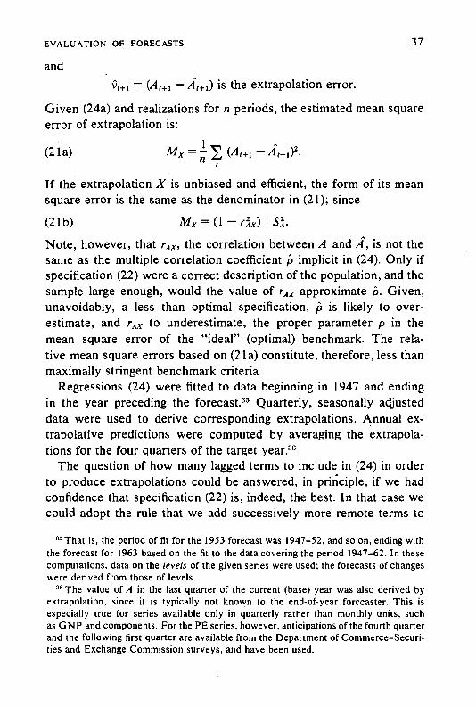
EVALUATION OF FORECASTS 37
and= — is the extrapolation error.
Given (24a) and realizations for n periods, the estimated mean squareerror of extrapolation is:
(21a) _At+i)2.
If the extrapolation Xis unbiased and efficient, the form of its meansquare error is the same as the denominator in (21); since(21b) = (1 — 'Si.Note, however, that the correlation between A and A, is not thesame as the multiple correlation coefficient implicit in (24). Only ifspecification (22) were a correct description of the population, and thesample large enough, would the value of rAx approximate Given,unavoidably, a less than optimal specification, is likely to over-estimate, and rAx to underestimate, the proper parameter p in themean square error of the "ideal" (optimal) benchmark. The rela-tive mean square errors based on (21a) constitute, therefore, less thanmaximally stringent benchmark criteria.
Regressions (24) were fitted to data beginning in 1947 and endingin the year preceding the forecast.35 Quarterly, seasonally adjusteddata were used to derive corresponding extrapolations. Annual ex-trapolative predictions were computed by averaging the extrapola-tions for the four quarters of the target year.36
The question of how many lagged terms to include in (24) in orderto produce extrapolations could be answered, in principle, if we hadconfidence that specification (22) is, indeed, the best. In that case wecould adopt the rule that we add successively more remote terms to
35That is, the period of fit for the 1953 forecast was 1947—52, and so on, ending withthe forecast for 1963 based on the fit to the data covering the period 1947—62. In thesecomputations, data on the levels of the given series were the forecasts of changeswere derived from those of levels.
The value of A in the last quarter of the current (base) year was also derived byextrapolation, since it is typically not known to the end-of-year forecaster. This isespecially true for series available only in quarterly rather than monthly units, suchas GNP and components. For the PE series, however, anticipations of the fourth quarterand the following first quarter are available from the Department of Commerce—Securi-ties and Exchange Commission surveys, and have been used.

38 ECONOMIC FORECASTS AND EXPECTATIONS
the right hand side of (24) until we used At_k, such that the additionalset At_k_I to (in our case, t — n is 1947) yields no further increasein the adjusted multiple correlation coefficient
In practice, again, maximization of will not necessarily minimizeExperiments with stopping rules on autoregressive equations
(24) of successively higher order showed that the addition of longerlags does reduce the over-all extrapolation error in some cases whereit does not increase ,E. Such reductions, however, are, on the whole,small. The experiments indicate that the smallest extrapolation errorsare obtained by using five-term lags for GNP and industrial produc-tion, and two-term lags for consumption and plant and equipment ex-penditures.37
Table 1-7 (columns 3 and 4, lines 1—8) shows the proportions ofsystematic error in the extrapolative forecasts and the co-efficients of correlation between the extrapolated and observedchanges (rAx). As would be expected, the autoregressive predictionsare largely free of significant biases: the systematic components aresmall, not only for the models selected here but typically also forthose with fewer or more lagged terms in the range covered in thesetests.38 The correlations rAx are high for the autoregressive predictionsof levels, but (except in the case of investment) rather low for changes.Here the results often differ considerably, depending on the numberof the lagged terms included in the models. But the models selected,which are those with the lowest values, also turn out, with onlyone exception, to be the models with the highest r4x values (comparecolumns 5 and 6, lines 1—8).
We conclude that the autoregressive extrapolations, while notnecessarily optimal, show a substantial margin of superiority over theusual naive models. This is partly because the former are less likelyto be biased than the latter, and partly because they are more efficient.A relatively small number of lags is sufficient to produce satisfactorybenchmarks in terms of minimizing
It should be noted that these particular conclusions are based on the entire forecastperiod 1953—63. The choice of numbers of lagged terms is thus ex post, utilizing moreinformation than was available to the forecaster. But, as Table 1-7 shows, the effects ofvarying lag periods on the mean square extrapolation errors are rather small, at least inthe selected data.
Only for the changes in industrial production did some of the X models yield sig-nificant bias proportions.

4.—
EVALUATION OF FORECASTS 39
EXTRAPOLATION ERRORS IN MULTIPERIOD FORECASTING
Consider a series that has an autoregressive representation (22).Suppose that, in addition to extrapolating one period ahead, we alsowant to extrapolate any number (k) of periods ahead: It can be shownthat an optimal (in the sense of minimum extrapolation error) extrapo-lation at t — k for k spans ahead is achieved by substitution of the asyet unknown magnitudes in the autoregression (22) by their extrapo-lated values:
(25) tAl_k = 135(t_IAt_k) + /32G_2A1_k) . . +
/3 kA 1-k + /3k+lA
For example, let k = 2: We substitute
= a + /31A1_2 + f32A1_3into(22a) A1= a+/31(A1_1 + +• . . +
obtaining
(26) A1 = a (1 + /3k) + + /32)A1_2 + (131/32 + f33)A1_3
+ (J3i€t_i E1).
According to (26), the mean square error of extrapolation in pre-dicting A1 at time t — 2 is the variance of + Given thestationarity assumptions underlying the autoregressive model (22),which state that El is not serially correlated and that the varianceof El_k 15 the same for all k, we have:
(27) = (1 +
It can be seen, by similar substitutions, that the mean square extrapo-lation error for any span (k) is equal to:
(28) hMX = (1 + + + • + .
40
=$çy1_3, (with Yo = 1).
For a sophisticated mathematical treatment of this topic, see [II].For the derivation and a more intensive study of these patterns and their implica-
tions in forecasting see Mincer's "Models of Adaptive Forecasting" in this volume.

40 ECONOMtC FORECASTS AND EXPECTATIONS
We see that in stationary linear autoregressive series, the extrapola-tion error kMX increases with lengthening of the span k. The rate atwhich the predictive power of extrapolations deteriorates as the targetis moved further into the future depends on the patterns of coefficientsin the autoregression (22) (see reference in footnote 40).
To the extent that forecasts P rely on extrapolations, and the latterare based on, or can be represented by, linear autoregressions, wewould expect their accuracy to deteriorate with lengthening of thespan. There is, indeed, ample evidence that forecasts deteriorate withlengthening span.
This can be seen in Table 1-8, where mean square errors of fore-casts kMp and of extrapolation kMx increase with span k (columns 1through 4). As in the previously observed case k = 1, we now alsofind that forecast errors are generally smaller than extrapolationerrors in multispan forecasting.
Accordingly, the relative mean square errors are, without excep-tion, less than one (column 5). On the whole, the RM indexes arelarger for changes than for levels, indicating that forecasts have a com-parative advantage in predicting levels, regardless of span.
The mean square errors of forecasts and of extrapolations increasewith span, as we expected. An interesting question is: Do forecastsor extrapolations deteriorate more rapidly? The answer is given by theRM indexes in Table 1-8 (column 5), which show a tendency to in-crease with span. With the exception of quarterly GNP forecasts(lines 1—8), this regularity is more closely observed in the correctedrelative mean square errors RMC (column 6).
Looking further into the components of RMC = 1 we see1 —
that the partials rApt decline with the extension of span (column 7),while rAx.p increases (column 8). Evidently, the contribution of theautonomous component of P to predictive efficiency tends to declinein longer-span forecasts. At the same time, the degree to which fore-casts fail to utilize the predictive power of extrapolations tends toincrease with lengthening of the span.
Our finding that the autonomous components of forecasts deter-iorate with span faster than the extrapolations can be explained bythe following: Consider the ingredients of general economic forecasts.In addition to extrapolations of some kind, forecasters use relations

EVALUATION OF FORECASTS 41
between the series to be predicted and known or estimated values ofother variables; various anticipatory data, such as investment inten-tion surveys and government budget estimates; and, finally, their ownpresumably informed judgments. Each of these potential sources offorecast is subject to deterioration with lengthening span. The fore-casting relations between time series involve lags of various lengths.Typically, the relations weaken as the lags are increased. Most indi-cators and anticipatory data have relatively short effective forecast-ing leads beyond which their usefulness declines. Informed judgmentsand estimates will probably also serve best over short time ranges.Hence, a hypothesis that P would tend to improve relative to X forthe longer spans may well be contradicted by the data, and apparentlyoften is, according to Table 1-8.
Evidence presented elsewhere indicates that similar results are alsoobtained in comparing forecasts with certain simple trend extrapola-tions: The errors of forecasts tend to increase more than the errorsof these extrapolations. Relative to the naive models Ni and N2,however, the performance of most forecasts improves with extensionsof the span.4' Clearly, these models fail to provide trend projections.
Such projections become more useful with lengthening of span.Forecasts do in part incorporate trend projections. Still greater re-liance on them might improve forecasting performance in the longerspans.
SUMMARY
This study is an exposition of certain criteria and methods of evalu-ating economic forecasts, and provides examples of their empiricalapplication. The forecasts are sets of numerical point predictions,classified by source (individuals or groups), subject (time series foraggregative economic variables), and span (time from issue to targetdate).
Analysis of absolute forecast errors proceeds from a simple scatterdiagram and a regression of realizations on predictions. A forecast isunbiased if the mean values of the predictions and the realizations areequal, that is, if the average error is zero. It is efficient if the pre-
Zarnowitz [13].

42 ECONOMIC FORECASTS AND EXPECTATIONS
TABLE 1-8. Comparisons of Forecasts and Extrapolations for Varying Spans,195 3—63
RelativeMean Square
ErrorPartial
Span RM RMC Correlation
LineCode and Type
of Forecast a
ofFore-cast b
k
Mean Square Error (col. I (col. 2÷ ÷
col. 3) col. 4)(5) (6)
Coefficients
r4py(7) (8)
kMP kMcp kMX(1) (2) (3) (4)
A. Gross National Product
Quarterly forecasts,1953—63
Forecast G (20)1 Level 1 83.6 68.5 205.2 160.6 .407 .427 .771 —.228
2 Level 2 99.5 62.3 340.3 247.2 .292 .252 .873 —.2343 Level 3 243.0 223.1 512.3 498.6 .474 .447 .751 —.1624 Level 4 306.4 91.5 446.6 311.4 .686 .294 .840 .048
5 Change 1 36.9 29.3 52.7 44.0 .700 .666 .589 .1386 Change 2 89.0 71.1 119.5 100.0 .744 .712 .614 .3527 Change 3 306.8 252.0 377.0 377.0 .814 .668 .599 .0798 Change 4 211.4 136.7 221.0 191.4 .957 .714 .614 .357
Semiannual forecasts, .
1955—63
Forecast D (16)
9 Level 1 160.0 87.6 265.0 186.6 .604 .470 .728 .04810 Level 2 327.1 211.3 429.8 288.7 .761 .732 .562 .254
II Change I 67.1 61.9 143.9 107.0 .466 .579 .649 .02012 Change 2 223.0 181.2 273.2 203.6 .816 .890 .390 .217
Forecast G (16)13 Level 1 79.5 45.5 265.0 186.6 .300 .244 .888 —.36014 Level 2 169.0 87.2 429.8 288.7 .393 .302 .836 —.016
15 Change 1 53.2 38.0 143.9 107.0 .370 .355 .804 .075
16 Change 2 179.1 99.2 273.2 203.6 .656 .487 .719 .097
(continued)

EVALUATION OF FORECASTS 43
TABLE 1-8 (concluded)
RelativeMean Square
. ErrorPartial
Span RM RMC Correlation
LineCode and Type
of Forecast a
of Mean Square ErrorFore-cast b kMp
k (1) (2) (3) (4)
(cot. I (col. 2÷ ÷
cot. 3) cot. 4)(5) (6)
Coefficients
(7) (8)
B. Index of Industrial ProductionQuarterly forecasts,1953-63
Forecast G (19)17 Level 1 14.4 10.3 68.6 60.4 .210 .171 .922 —.35218 Level 2 25.4 20.0 100.3 80.9 .253 .247 .868 .00219 Level 3 88.4 36.4 113.9 94.1 .776 .387 .786 .12120 Level 4 73.7 52.3 163.0 108.8 .452 .480 .730 .165
21 Change 1 9.9 9.0 18.9 18.4 .524 .488 .743 .28722 Change 2 23.8 23.6 51.1 40.1 .467 .588 .698 .35623 Change 3 49.9 45.9 83.2 59.3 .600 .773 .593 .40224 Change 4 76.5 66.8 126.6 79.1 .604 .845 .528 .383
Semiannual forecasts,1955—63
Forecast D (16)25 Level 1 29.1 29.1 85.9 78.9 .339 .369 .764 .10426 Level 2 69.7 69.7 165.8 123.3 .420 .570 .667 .38227 Change 1 32.3 32.3 56.4 49.0 .573 .659 .537 .26228 Change 2 75.7 75.7 136.4 94.4 .555 .802 .455 .369
Forecast G (16)29 Level 1 18.0 14.9 85.9 78.9 .210 .189 .901 —.06930 Level 2 70.3 55.9 165.8 122.3 .424 .457 .751 .21031 Change 1 40.0 17.2 56.4 49.0 .708 .352 .808 .11432 Change 2 75.6 64.4 136.4 94.4 .554 .682 .615 .300
a Number of predictions for each forecast set per span is given in parentheses.Quarterly forecasts refer to levels and changes in the given series one, two, three, and four quarters
following the quarter (base period) in which the forecast was made. Semiannual forecasts refer to levelsand changes in the series one and two halves following the half (base period) in which the forecast was made.Changes are computed from the base period to the relevant quarter (or half).
Lines 1—16, billions of dollars squared; lines 17—32, index points squared (1947—49 100).

44 ECONOMIC FORECASTS AND EXPECTATIONS
dictions are uncorrelated with errors, so that the slope of the re-gression equals unity. A convenient summary measure is the meansquare error, which includes the variance of the residuals from thatregression as well as two other components reflecting the bias andinefficiency of the forecast, respectively. The mean component iszero for an unbiased forecast, and the "slope component" is zero foran efficient forecast; hence, if the predictions are both unbiased andefficient, the mean square error reduces to the residual variance.
In dealing with limited samples of predictions and realizations, sta-tistical tests are necessary to ascertain whether the forecasts aresignificantly biased or inefficient, or both. Measures of accuracy anddecomposition of mean square errors are presented for several sets ofbusiness forecasts, along, with test statistics for lack of bias and forefficiency. Bias is found most often in predictions of GNP and con-sumption. The residual variance accounts for most of the total meansquare error, while the slope component is the smallest.
Another fact revealed by the accuracy analysis of forecasts ofchanges is the tendency to underestimate the absolute size of changes,a tendency reported in other studies. This tendency may be due tounderestimation of levels in upward-trending series, or to an appar-ent underestimation of the variance of actual changes. The latter istheoretically implicit in efficient forecasting and is, therefore, not initself a forecasting defect. In the forecasts examined here, however,it is the underestimation of levels that mainly accounts for the observedunderestimation of changes. There is also evidence that increasesin series with strong upward trends are likely to be underpredicted, butthis is not so for decreases in series with little or no such trends. Inshort, the one established phenomenon is tendency toward a con-servative estimation of growth prospects.
Extrapolations of past values are relatively simple and inexpensiveforecasting procedures which can be.deflned and reproduced. A fore-cast may be judged satisfactory according to its absolute errors; butif a less costly extrapolation is about as accurate, the comparativeadvantage is on the side of the extrapolation. We compared forecasterrors to extrapolation errors in the form of a ratio of the two meansquare errors. This ratio, the relative mean square error, can thus beviewed as an index of the marginal rather than total productivity ofbusiness forecasting. Moreover, it provides a degree of commensura-

EVALUATION OF FORECASTS 45
bility for diverse forecasts whose absolute errors cannot be meaning-fully compared.
Optimal, that is predictively most accurate, extrapolations are diffi-cult to construct. As convenient substitutes, we use autoregressiveextrapolations of a relatively simple sort, based on information avail-able to the forecaster. Unlike the naive models, which have beenwidely used as standard criteria of forecast evaluation, the autore-gressive benchmarks take partial account of the statistical structureof the time series to be predicted. They are largely free of bias anddefinitely superior to the naive models.
It is possible for a forecast to be less accurate than the benchmarkextrapolations, yet to be superior after correction for bias and in-efficiency. Even without such corrections, our collection of forecastsshows a consistently greater accuracy than autoregressive predic-tions.42 The margin of superiority is increased when corrected fore-casts are compared to corrected extrapolations.
Extrapolation is an alternative, but not an exclusive, method of fore-casting. It is, to some degree, incorporated in the business forecasts,and, to that degree, implicit extrapolation errors are a part of ob-served forecast errors. Our analysis permits us to decompose observedforecasts into extrapolative and other (autonomous) components, andto estimate the relative contributions of each to the predictive accu-racy of the forecast.
It is, of course, the autonomous component that is responsible forthe superior efficiency of forecasts over the benchmark extrapolations.At the same time, we find that available extrapolative information islargely utilized by forecasters. The extrapolative component of fore-casting is clearly more pronounced in strongly trending and relativelysmooth series than in others.
In the final section we extend our accuracy analyses to multispanforecasting. We compare errors of forecasting one quarter to fourquarters ahead. On the average, forecast errors increase with lengthof predictive span. One reason for this is that forecasts consist, inpart, of extrapolations whose accuracy declines for more distant tar-get dates. However, longer-term forecasts are generally worse than
42 Some other forecasts, however, particularly those for GNP components and longerspans, were found to be inferior to extrapolative benchmark predictions; see Zarnowitz[13, pp. 86—104].
46 ECONOMIC FORECASTS AND EXPECTATIONS
the short ones, when compared with such extrapolations. Evidently,the predictive power of the autonomous components of forecastsdeteriorates more rapidly with lengthening span. In addition, the po-tential of extrapolative prediction is utilized to a lesser degree bythe longer-span forecasts. Such forecasts, therefore, can gain from in-creased reliance on trend projection.
REFERENCES
[1] Alexander, S. S.. and Stekier, H. 0., "Forecasting Industrial Produc-tion— Leading Series vs. Autoregression," Journal of Political Economy,August 1959.
[2] Christ, Carl, "A Test of an Econometric Model forthe U.S. 192 1—1947,"in Conference on Business Cycles, NBER, New York, 1951.
[3] Cunnyngham, Jon, "The Short-Term Forecasting Ability of EconometricModels," NBER, unpublished.
[4] Hickman, W. Braddock, "The Term Structure of Interest Rates: AnExploratory Analysis," NBER, 1942, mimeographed.
[5] Muth, J. F., "Rational Expectation and the Theory of Price Movements,"Econometrica, July 1961.
[6] Okun, A. M., "A Review of Some Economic Forecasts for 1955—57,"Journal of Business, July 1959.
[7] Theil, H., Applied Economic Forecasting, Chicago, 1966.[8] , Economic Forecasts and Policy, Amsterdam, 1961.[9] , Optimal Decision Rules for Government and Industry, Amster-
dam, 1964.[10] Wald, A., and Mann, H. B., "On the Statistical Treatment of Linear
Stochastic Difference Equations," Econometrica, July 1943.[11] Whittle, P., Prediction and Regulation, London, 1963.[12] Yaglom, A. M., Stationary Random Functions, Englewood Cliffs, N.J.,
1962.[13] Zarnowitz, Victor, An Appraisal of Short-Term Economic Forecasts,
Occasional Paper 104, New York, NBER, 1967.