1

EPRI Lightning ProtectionDesign Workstation

Tom McDermottElectrotek Concepts, Inc.

2000 Winter Power Meeting

LPDW v5 Components

• Includes 1988-97 flash data from theNational Lightning Detection Network

• CFlash for underground distribution (new)• DFlash for overhead distribution• TFlash for overhead transmission• LPData.exe - manages main database• On-line reference

2

LPDW History• 1992 v1 Release (DFlash)• 1994 v2 Release

– DFlash pole drawing– MultiFlash for transmission

• 1997 v4 Release– brand new TFlash for transmission– multiple circuits in DFlash

• 1999 v5 - brand new CFlash for cables

DFlash Features• Lightning Flash Data (EPRI RP 2431)

– Ground Flash Density maps– Peak currents of the first stroke

• Pole Insulation Strength analysis (EPRI RP 2874)• Shielding

– Overhead shield wires– Nearby trees and houses

• Surge Arresters at various spacings• Pole Ground Resistance• Transformer Protection (lead length, low-side surges)• Equipment Inventory

3

DFlash Line Flashover Calculation

TransientsProgram

Critical Currentsto Cause Flashover Electrogeometric

ModelCFO

Volt-timeModel

Arresters

Stroke Front Times

Framing

Insulators

ImpulseResistance

Grounding

Distribution of First-StrokePeak Currents

Flashovers

Ground Flash Density

Line Length

Nearby Objects

Line Section

Pole Design

DFlash Pole Design Dialog

4

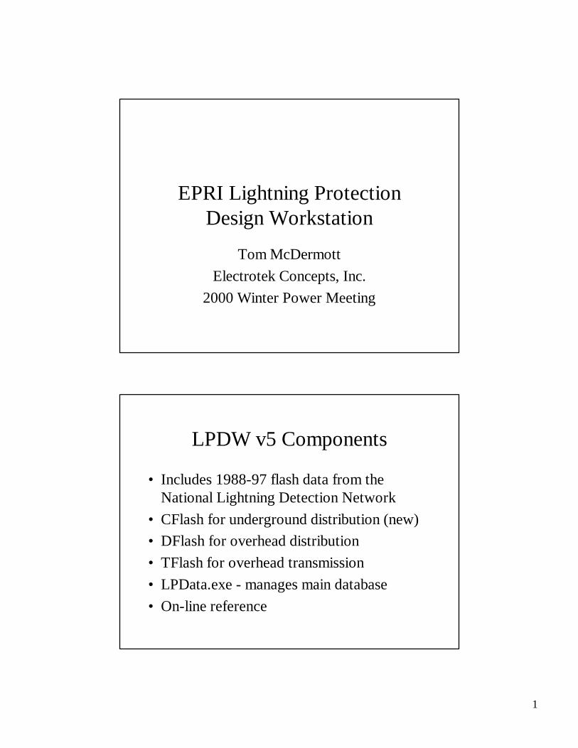
DFlash Conductor and InsulatorSpecification

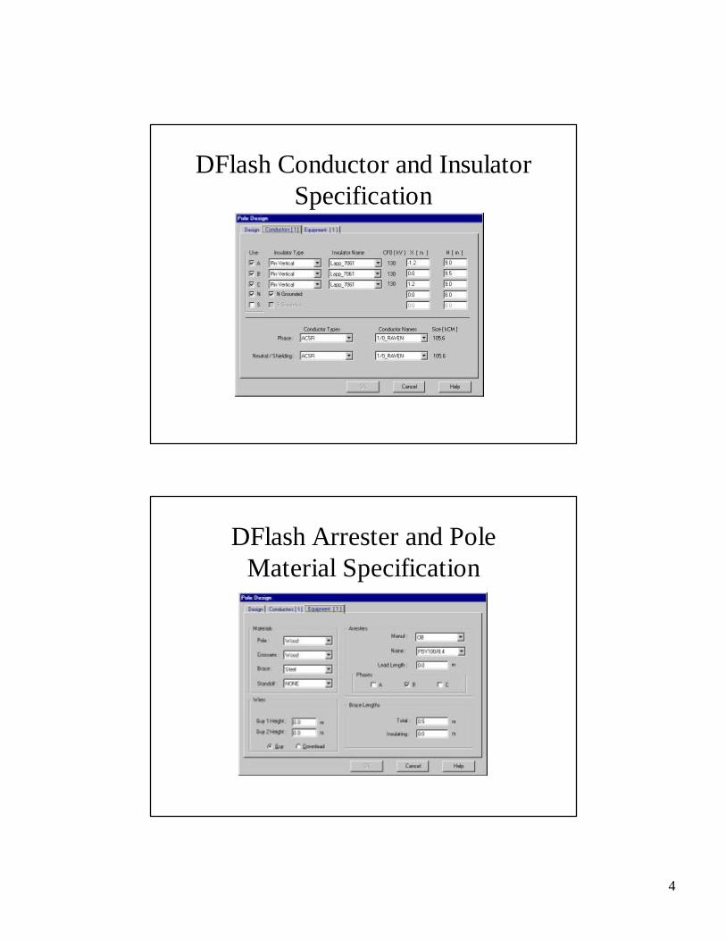
DFlash Arrester and PoleMaterial Specification

5

Distribution of Total VoltageAcross Pole Insulation

CFO Added Values

6

Sample Pole CFO [kV]

Phase No Arrester Phase B ArresterA 370 340B 439 130C 370 340

Time to Flashover• CFO is based on a 1.2 x 50 µs standard

laboratory test waveshape• Destructive Effect (Dflash v1-4.1):

• Leader Progression Model (Dflash v5):

−= 0

)()(/ E

xte

tKedtdx where K = propagation constantE0 = breakdown gradientx = unbridged gap lengthe(t) = voltage across gap

( )∫ −= dtVeDE bβ

7

Air-Porcelain Volt-Time CurvesTime-lag Curves for 100 kV CFO

0

50

100

150

200

250

0 2 4 6 8

Time to Flashover [us]

Cres

t Vol

tage

[kV] DE 1-cos

DE Concave

LPM 1-cos

LPM Concave

CFO Guidelines for Dflash

• Large impact on flashovers from inducedvoltages - want CFO at least 300 kV

• Not much effect on direct-stroke flashovers(it’s hard to make overhead shield wireswork on distribution lines)

• Steel and concrete structural elements hurt• Guy wires, downleads, fuse cutouts, and

switches also hurt

8

DFlash Line Section Dialog

DFlash Line Section Flashovers

9

Sample Line Flashover Results100 km, GFD=1, 9.1 first strokes to line/year0.188 shielding failure flashovers in all cases

Arrester Ground Stroke to B ExcessSpacing 1-φ FO 2,3-φ FO EnergyNone 50 8.910 0.000 0.000Every 2 50 4.368 0.985 3.130Every 1 50 0.000 1.969 5.311None 10 8.910 0.000 0.000Every 2 10 4.516 0.126 3.841Every 1 10 0.000 0.373 6.907

Arresters at Every GroundVp = Vn + Ea

Vn = I * R

RI

Ea Ea

Stroke

(Ground resistance makes no difference)

10

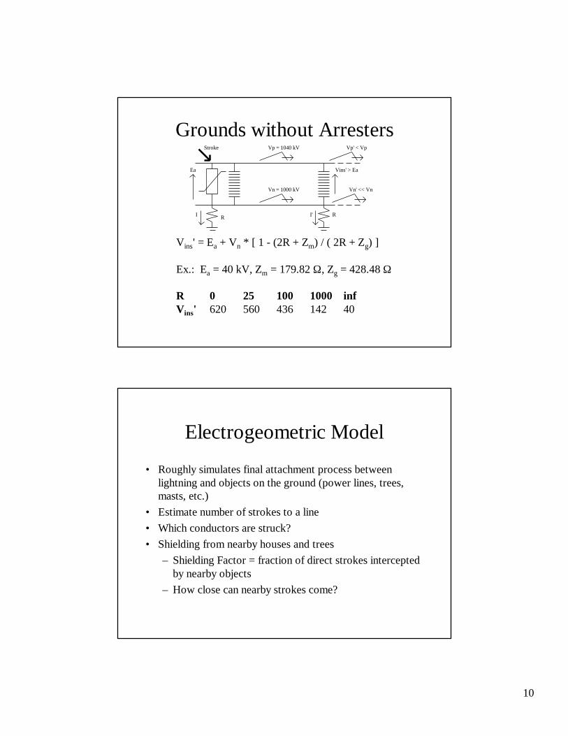
Grounds without ArrestersVp = 1040 kV

Vn = 1000 kV

RI

Ea Vins' > Ea

Stroke

RI'

Vp' < Vp

Vn' << Vn

Vins' = Ea + Vn * [ 1 - (2R + Zm) / ( 2R + Zg) ]

Ex.: Ea = 40 kV, Zm = 179.82 Ω , Zg = 428.48 Ω

R 0 25 100 1000 infVins' 620 560 436 142 40

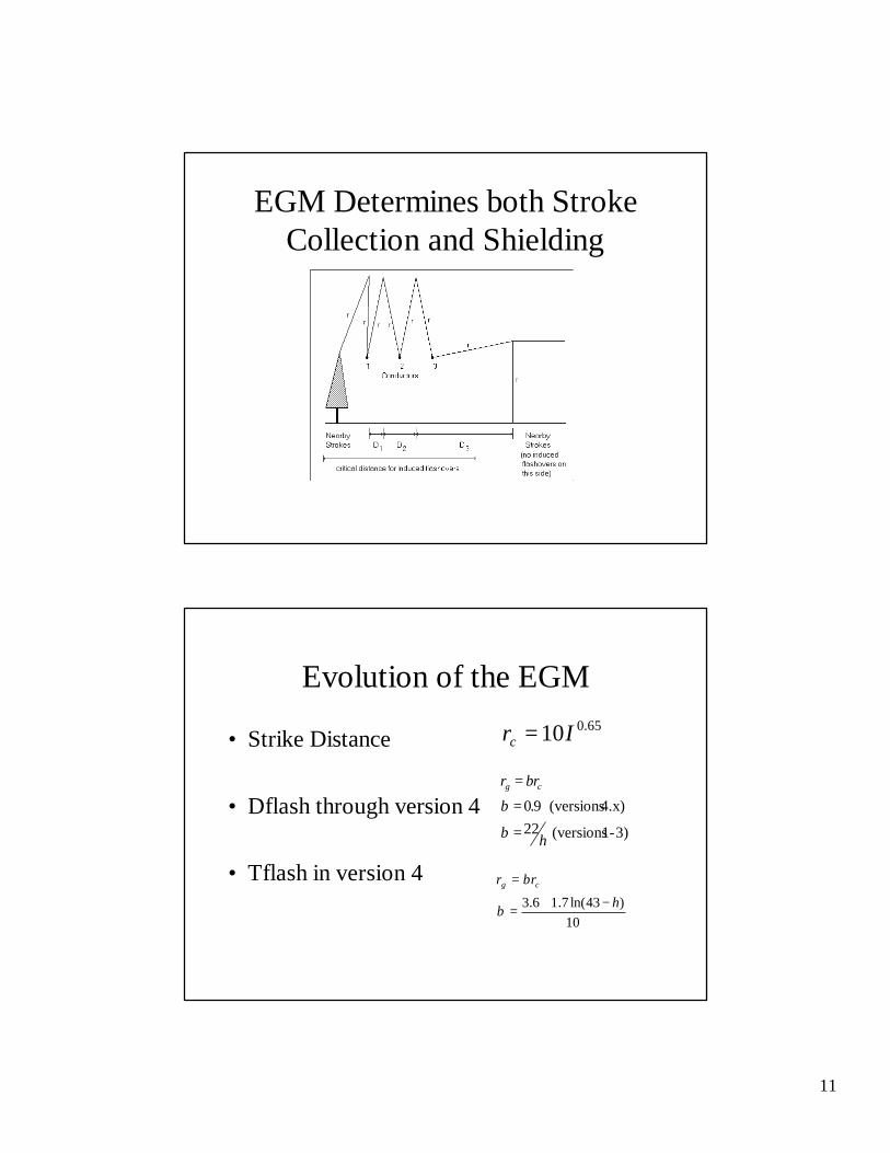
Electrogeometric Model

• Roughly simulates final attachment process betweenlightning and objects on the ground (power lines, trees,masts, etc.)

• Estimate number of strokes to a line• Which conductors are struck?• Shielding from nearby houses and trees

– Shielding Factor = fraction of direct strokes interceptedby nearby objects

– How close can nearby strokes come?

11

EGM Determines both StrokeCollection and Shielding

Evolution of the EGM

• Strike Distance

• Dflash through version 4

• Tflash in version 4

3)-1 (versions 224.x) (versions 9.0

h

rr cg

===

ββ

β

65.010Irc =

10)43ln(7.16.3 h

rr cg

−+=

=

β

β

12

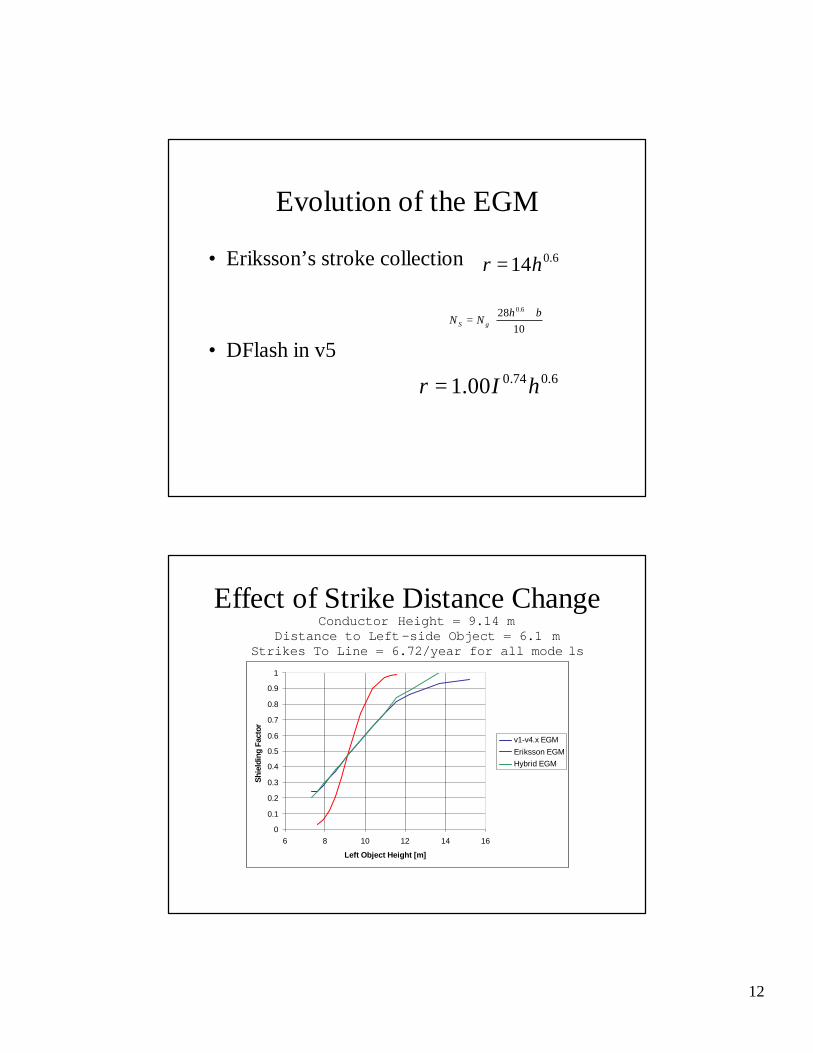
Evolution of the EGM

• Eriksson’s stroke collection

• DFlash in v5

6.014hr =

+=

1028 6.0 bh

NN gS

6.074.000.1 hIr =

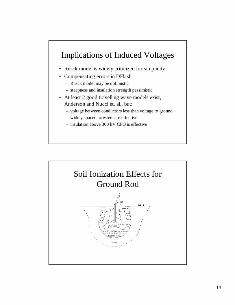
Effect of Strike Distance ChangeConductor Height = 9.14 m

Distance to Left-side Object = 6.1 m Strikes To Line = 6.72/year for all mode ls

0

0.1

0.2

0.3

0.4

0.5

0.6

0.7

0.8

0.9

1

6 8 10 12 14 16

Left Object Height [m]

Shie

ldin

g Fa

ctor

v1-v4.x EGMEriksson EGMHybrid EGM

13

Implications of the EGM• Need to match shielding with stroke collection• Median current of strokes to the line increases

with height• NLDN current distribution may become preferred

data source, median to flat ground is in the 20’s ofkA

• A leader progression model (Rizk, Dellera andGarbagnati) might be better

• Could use a 3D model for nearby objects

ApplyingRusck’s Model

Maximum Voltage:

Voltage for 1-kA stroke, 1foot away from a conductor1 foot above ground:

Critical distance for anearby stroke:

14

Implications of Induced Voltages• Rusck model is widely criticized for simplicity• Compensating errors in DFlash

– Rusck model may be optimistic– steepness and insulation strength pessimistic

• At least 2 good travelling wave models exist,Anderson and Nucci et. al., but:– voltage between conductors less than voltage to ground– widely spaced arresters are effective– insulation above 300 kV CFO is effective

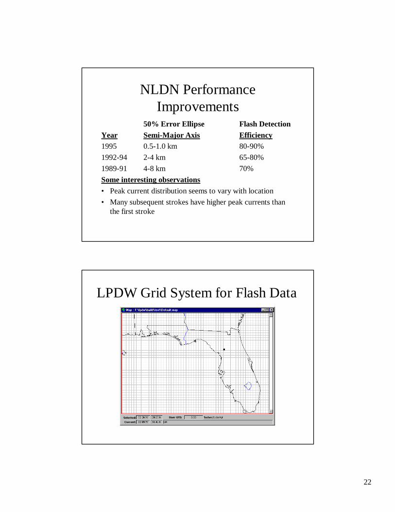
Soil Ionization Effects forGround Rod

15

Weck’s Approximation

Effect of Pole Ground on theInduced Voltage

V' = V 1 - (hg / hp) [Zm / (2R + Zg)]Vn = V (hg / hp) * [2R / (2R + Zg)]Vins = V' - Vn

= V 1 - (hg / hp) [(2R + Zm) / (2R + Zg)]

16

Example: Induced Voltage withPole Ground

hp = 30 ft hn = 24 ft Zg = 500 ΩZm = 150 Ω R = 50 Ω CFO = 300 kV

Suppose V = 300 kV from nearby stroke, on a conductor 30 ft above ground

Vins = 300 [1 - (24/30)] = 60 kV at ungrounded poles

V' = 300 1 - (24/30) * [150/(2 * 50 + 500)] = 240 kV

Vn = 300 (24/30) * [(2 * 50)/(2 * 50 + 500)] = 40 kV

Vins = 240 - 40 = 200 kV at grounded poles

Crest Current Distributions

17

Front of Wave Distributions

Stroke Front Time Options

0

0.5

1

1.5

2

2.5

3

3.5

0 50 100 150 200 250 300First-stroke Peak Curent [kA]

Front Time [microsecnds]

Cigre/NLDN

IEEE

18

Arrester VI Characteristics

Arrbez Turn-On Conductance and Inductance Model, Uref = 0.051, L = 0.3 µH,20 kA, 1x20 Discharge Current

Arrester Time Dependence

19

Stroke Tail Time• Arrester energy approximation for an

Exponential tail– Time Constant: τ = 1.44 T50

– Energy: E = I V τ– Charge: Q = I τ

• For median Q = 4.65 and I = 31.1, τ = 150µs, or T50 = 104 µs

• Berger’s basic data was 77.5 µs

Arrester Energy Sharing

Arrester Discharge Currents with 37 Parallel Arresters

20

Arrester Energy SharingArrester Energy Sharing, Single-Phase Line, 150-ft

Span

0

10

20

30

40

50

0 5 10 15 20 25 30 35 40

Number of Arresters

Max

Ene

rgy

[kJ]

39.04 14.54 10.26

Effect of Arrester on InducedVoltage

CFO = FOWPL + 2 t Sv= FOWPL + 2 L Vpk / Tfront c

The "unprotected" induced voltage required to cause flashover is:Vpk = (CFO - FOWPL) * Tfront * c / (2 L)

21

Example: Induced Voltage withArresters and Grounds

FOWPL = 45 kV L = 150 ft/spanTfront = 1 µsec c = 984 ft/µsecCFO = 300 kV R = 50 Ω

Arr. Sep. L [ft] Vpk for Vins >= 300 kV

0 infinite

150 1255 kV

300 627 kV

infinite 450 kV

(1500 kV for ungrounded)

IMPACT Sensors in the NLDN• Combines magnetic direction finding with time-

of-arrival• Time of Arrival (TOA) modified to use absolute

times from GPS clock, changes hyperbolas torange circles

• Improved hardware, calibration, adjustments, andalgorithms

• The new NLDN is roughly half IMPACT, halfTOA, and includes Canada

22

NLDN PerformanceImprovements

50% Error Ellipse Flash DetectionYear Semi-Major Axis Efficiency1995 0.5-1.0 km 80-90%1992-94 2-4 km 65-80%1989-91 4-8 km 70%Some interesting observations• Peak current distribution seems to vary with location• Many subsequent strokes have higher peak currents than

the first stroke

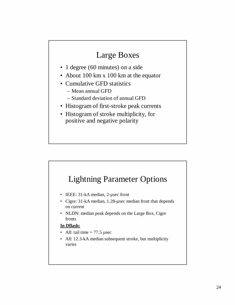
LPDW Grid System for Flash Data

23

Small Boxes

• 10 minutes on a side• About 16 x 16 km at the equator• Cumulative flash counts for positive and

negative polarity• Use for local ground flash density (GFD)• Line Sections and Towers are located in

small boxes

GFD from NLDN

24

Large Boxes• 1 degree (60 minutes) on a side• About 100 km x 100 km at the equator• Cumulative GFD statistics

– Mean annual GFD– Standard deviation of annual GFD

• Histogram of first-stroke peak currents• Histogram of stroke multiplicity, for

positive and negative polarity

Lightning Parameter Options

• IEEE: 31-kA median, 2-µsec front• Cigre: 31-kA median, 1.28-µsec median front that depends

on current• NLDN: median peak depends on the Large Box, Cigre

frontsIn Dflash:• All: tail time = 77.5 µsec• All: 12.3-kA median subsequent stroke, but multiplicity

varies

25

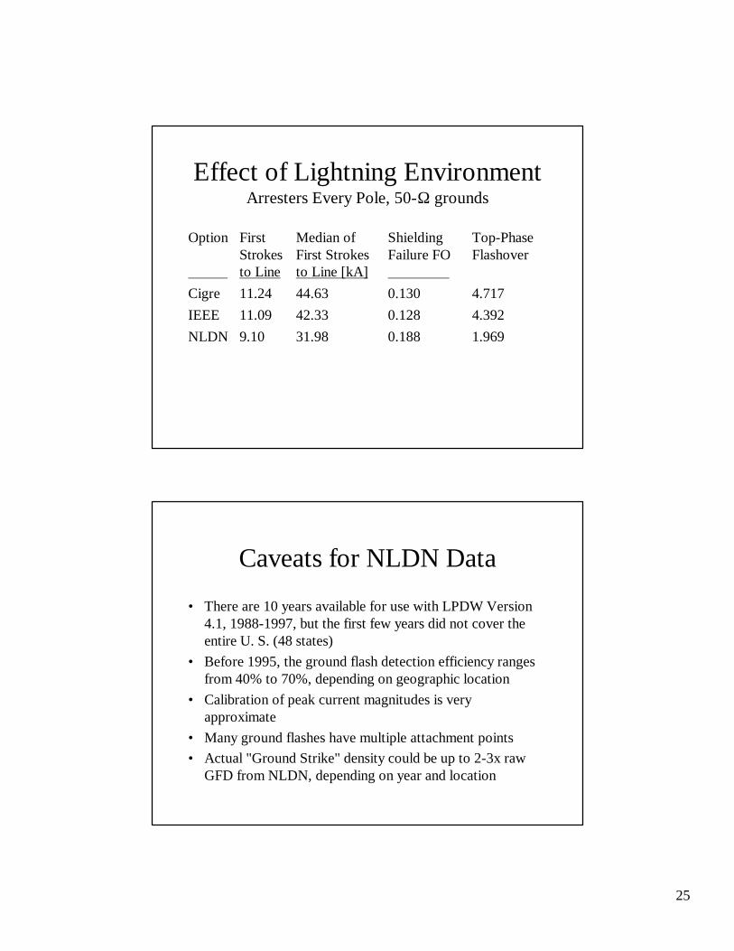
Effect of Lightning EnvironmentArresters Every Pole, 50-Ω grounds

Option First Median of Shielding Top-PhaseStrokes First Strokes Failure FO Flashover

to Line to Line [kA] Cigre 11.24 44.63 0.130 4.717IEEE 11.09 42.33 0.128 4.392NLDN 9.10 31.98 0.188 1.969

Caveats for NLDN Data

• There are 10 years available for use with LPDW Version4.1, 1988-1997, but the first few years did not cover theentire U. S. (48 states)

• Before 1995, the ground flash detection efficiency rangesfrom 40% to 70%, depending on geographic location

• Calibration of peak current magnitudes is veryapproximate

• Many ground flashes have multiple attachment points• Actual "Ground Strike" density could be up to 2-3x raw

GFD from NLDN, depending on year and location

26

Fault Analysis and LightningLocation System (FALLS)

• First release in 1995• GIS-based (MapInfo)• Uses NLDN flash or stroke data with time-

correlated power system events• Small-area GFD and stroke parameter maps• Asset exposure and reliability analysis

– difference between “hot lightning areas” and “hotflashover areas”

• Solaris/Sybase server, Solaris or NT client

TFlash Features

• Complete modeling of the line, tower-by-tower• Ground rods, radial and continuous counterpoise

with impulse resistance• Transmission line surge arresters• Shielding from nearby objects• Transmission line surge arresters• Corona effects• Tower surge impedance

27

Improvements for Version 6

• Map based on commercial GIS• Improve archived NLDN data, with stroke

current distributions in the 10-minute boxes• Internationalization, allow other sources of

lightning data• Pole model options (underbuild, H-frame)• More access to modeling options

Future Work

• Revised/redone electrogeometric model• Better characterize the arrester energy

discharge capability• CFO added from fiberglass guy insulators

(needs laboratory testing)• Time-domain simulation of induced

voltages