the emergent properties of spatial self-organization - rug.nl fileplease check the document ......
TRANSCRIPT

University of Groningen
The emergent properties of spatial self-organizationLiu, Quan-Xing
IMPORTANT NOTE: You are advised to consult the publisher's version (publisher's PDF) if you wish to cite fromit. Please check the document version below.
Document VersionPublisher's PDF, also known as Version of record
Publication date:2013
Link to publication in University of Groningen/UMCG research database
Citation for published version (APA):Liu, Q-X. (2013). The emergent properties of spatial self-organization: A study of patterned mussel beds.Groningen: s.n.
CopyrightOther than for strictly personal use, it is not permitted to download or to forward/distribute the text or part of it without the consent of theauthor(s) and/or copyright holder(s), unless the work is under an open content license (like Creative Commons).
Take-down policyIf you believe that this document breaches copyright please contact us providing details, and we will remove access to the work immediatelyand investigate your claim.
Downloaded from the University of Groningen/UMCG research database (Pure): http://www.rug.nl/research/portal. For technical reasons thenumber of authors shown on this cover page is limited to 10 maximum.
Download date: 25-05-2019

Chapter 3
Phase separation explains a new class
of self-organized spatial patterns in
ecological systems
Self-organization is a process in which pattern at theglobal level of a system emerges solely from numerousinteractions among the lower-level components of thesystem. Moreover, the rules specifying interactionsamong the systems components are executed usingonly local information, without reference to the globalpattern.
According to Scott Camazine et al. (2003)
This chapter is based on the manuscript: Q.-X. Liu, A. Doelman, V. Rottschafer, M. d. Jager,
P. M.J. Herman, M. Rietkerk, and J. v.d. Koppel – “Phase separation explains a new class of
self-organized spatial patterns in ecological systems,” Proc. Natl. Acad. Sci. USA, vol. 110 (29)
11905-11910, doi: 10.1073/pnas.1222339110, 2013.

48 Phase separation in ecological systems
Abstract
Turing’s activator-inhibitor principle has been the central paradigmfor explaining regular, self-organized spatial patterns in ecology.According to this principle, local activation combined with long-range inhibition of growth and survival is an essential prerequisitefor the formation of regular ecological patterns. Here, we revealdensity-dependent motion of animals as a new mechanism for self-organization in ecology, and show that it conforms to the principleof phase separation in physics. The basis of this mechanism is aswitch from dispersal to aggregation with increasing density. First,using experiments with self-organizing mussel beds, we derive anempirical relation between animal movement speed and local animaldensity. Second, we incorporate this relation in a partial differentialequation, and show that this model corresponds mathematically to thewell-known Cahn-Hilliard equation for phase separation in physics.Third, we show that the assumptions and predictions of this modelwith regard to development of patterns are in close agreement with theresults of our experiments and field observations. Hence, our resultsuncover a new principle for ecological self-organization, where motionrather than activation and inhibition processes explains spatial patternformation.

Chapter 3 49
Introduction
The activator-inhibitor principle, originally conceived by Turing in1952 (Turing, 1952), and further developed by Belousov (Belousov,
1959), Zhabnotinsky (Zhabotinsky, 1964) and Meinhardt (Meinhardt, 1982)provided a potential theoretical explanation for the occurrence of regularpatterns in biology (Murray, 2002; Kondo and Miura, 2010; Maini, 2003) andchemistry (Zhabotinsky, 1964; Castets et al., 1990; Ouyang and Swinney,1991). In the past decades, this principle has been applied to a wide rangeof ecological systems, including arid bush lands (Klausmeier, 1999; van deKoppel and Crain, 2006; von Hardenberg et al., 2001; Rietkerk et al., 2002;Borgogno et al., 2009), mussel beds (van de Koppel et al., 2005; Liu et al.,2012), and boreal peat lands (Eppinga et al., 2009; Rietkerk and Van deKoppel, 2008). The activator-inhibitor principle, where a local positive,activating feedback interacts with large-scale inhibitory feedback to drivespatial differences in growth, birth, mortality, respiration or decay, explainsthe spontaneous emergence of regular spatial patterns. These patterns mayhave important emergent effects on the functioning of ecosystems, such asincreased growth efficiency, resource utilization and ecosystem resilience,independent of the organizational level (Liu et al., 2012; Pringle et al., 2010;Kondo and Miura, 2010; Rohani et al., 1997; Sole and Bascompte, 2006).
Physical theory offers an alternative mechanism for pattern formation,proposed by Cahn and Hilliard in 1958 (Cahn and Hilliard, 1958). Theypointed at the possibility that density-dependent rates of dispersal wouldlead to separation of a mixed fluid into two phases that are separated indistinct spatial regions, subsequently leading to pattern formation. Theprinciple of density-dependent dispersal, switching between dispersion andaggregation as local density increases, has become a central mathematicalexplanation for phase separation in many fields (Bray, 2002) such asmultiphase fluid flow (Falk, 1992), mineral exsolution and growth (Kuhland Schmid, 2007), and biological applications (Cohen and Murray, 1981;Chomaz et al., 2004; Khain and Sander, 2008; Cates et al., 2010; Liu et al.,2011). However, while aggregation due to individual motion is a commonlyobserved phenomenon within ecology, application of the Cahn-Hilliard(CH) framework to explain pattern formation in ecological systems is absentboth in terms of theory and experiments (Cohen and Murray, 1981; Cateset al., 2010).

50 Phase separation in ecological systems
Here, we apply the concept of phase separation to the formation ofspatial patterns in the distribution of aggregating mussels. On intertidalflats, establishing mussel beds exhibit spatial self-organization by forminga pattern of regularly spaced clumps. By so doing, they balance optimalprotection against predation with optimal access to food, as demonstratedin a field experiment (van de Koppel et al., 2008). This self-organizationprocess has been attributed to the dependence of the speed of movementon local mussel density (van de Koppel et al., 2008). Mussels move athigh speed when they occur in low density and decrease their speedof movement once they are included in small clusters. However, whenoccurring in large and dense clusters, they tend to move faster again,due to food shortage. Mussel pattern formation is a fast process, givingrise to stable patterning within the course of a few hours, and clearly isindependent from birth or death processes (Figure 3.1A and B). Althoughmussel pattern formation at centimeter scale was successfully reproducedby an empirical individual-based model (van de Koppel et al., 2008), to dateno satisfactory continuous model has been reported that can identify theunderlying principle in a general theoretical context.
In this paper, we present the derivation and analysis of a partialdifferential equation model based on an empirical description of density-dependent movement in mussels (van de Koppel et al., 2008), anddemonstrate that it is mathematically equivalent to the original model ofphase separation by Cahn and Hilliard (Cahn and Hilliard, 1958). We thencompare the predictions of this model with observations from real musselbeds and experiments with mussel pattern formation in the laboratory.
Results
Model Description
Mussel speed of movement was observed to initially decrease withincreasing mussel density, but to increase when the density exceeded thattypically observed in nature (Figure 3.1C). We analyzed the experimentaldata of movement speed as a function of mussel density statistically withtwo different models.

Chapter 3 51
A B
=⇒
0.0 0.2 0.4 0.6 0.8 1.0Rescaled mussel density
0.0
0.2
0.4
0.6
0.8
V(m
) and g
(m)
(cm
/min
)
Cg(m)
V(m)
0
0.2
0.4
0.6
0.8D
Figure 3.1: Pattern formation in mussels and statistical properties of the density-dependent movement of mussels under experimental laboratory conditions. (A)and (B), Mussels that were laid out evenly under controlled conditions on ahomogeneous substrate developed spatial patterns similar to ‘labyrinth-like’ after24 hours (images represent a surface of 60 cm by 80 cm). (C), Relation betweenmovement speed and density within clusters of 1, 2, 4, 6, 8, 16, 24, 32, 64, 80, 104,and 128 mussels (mussel density is rescaled, where 128 equals to 1). The blue linedescribes the rescaled second order polynomial fit with Eq.(3.1). The red line depictsthe effective diffusion g(m) of mussels as a function of the local densities accordingto the diffusion-drift theory. The circles show the original experiment data. (D),The numerical simulation of Eq. (3.4) implemented with parameters β = 1.89,D0 = 1.0, and κ1 = 0.1, simulating the development of spatial patterns from anear-uniform initial state.
The movement speed data was fitted to the equation
V(M) = aM2 − bM + c (3.1)
with a = 2.211, b = 2.102 and c = 0.6208 (Figure 3.1C; blue line). A linear

52 Phase separation in ecological systems
model proved not significant (P = 0.778). The quadratic model was overallsignificant (P < 0.001), where the coefficient for the second-order term washighly significant (t = 4.732, P < 0.0001), and the AIC-test showed that thequadratic model was highly preferable over the linear one (see Table 3.A1for details).
Based on this formulation, we now derive an equation for the changesin local density M of a population of mussels, in a 2-dimensional space.As the model describes pattern formation at time scales shorter than 24hours, growth and mortality (as factors affecting local mussel density) canbe ignored. Local fluxes of mussels at any specific location can therefore bedescribed by the generic conservation equation:
∂M
∂t= −∇ · J. (3.2)
Here J is the net flux of mussels, and ∇ = (∂x, ∂y) is the gradient in twodimensions. To derive the net flux J , we assume that mussel movement canbe described as a random, step-wise walk with a step size V that is a functionof mussel density, and a random, uncorrelated reorientation. In the case ofdensity-dependent movement, the net flux arising from the local gradient inmussel density can be expressed as (see Appendix 3.A)
Jv = − 1
2τ
(V(V +M
∂V∂M
))∇M, (3.3)
where τ is the turning rate (Schnitzer, 1993, see equation (4.14)). The “drift”term M∂V/∂M accounts for the effect of spatial variation in local musseldensity on the spatial flux of mussels. This term does not appear in the caseof density-independent movement, but its contribution is crucial when up-scaling the density-dependent movement of individuals to the populationlevel.
Following earlier treatments of biological diffusion as a result of indi-vidual movement (Murray, 2002, see p.408-416 for details), we complementthis linear diffusion term representing local movement by including higher-order (non-local) diffusion as Jnl = ∇(κ∆M) with nonlocal diffusioncoefficient κ. The non-local diffusion process has a relatively low intensity,and hence parameter κ is much smaller in magnitude than the localmovement coefficient in Eq.(3.3). We can now gather both fluxes into the

Chapter 3 53
total net flux rate in Eq.(3.2) to define the general rescaled conservationequation (see text in Appedix 3.A):
∂m
∂t= D0∇
[g(m)∇m− κ1∇(∆m)
]. (3.4)
Here, g(m) = v(m)(v(m) + m∂v(m)
∂m
), where v(m) = m2 − βm + 1
is a rescaled speed. D0 is a rescaled diffusion coefficient that describesthe average mussel movement, and κ1 is the rescaled non-local diffusioncoefficient. Rescaling at the basis of equation (3.4) is given by the followingrelations: g(m) = (m2 − βm + 1)(3m2 − 2βm + 1) with m =
√a/cM ,
D0 = c2
2τ , κ1 = 2τκc2
, and β = b/√ac. Here, β captures the depression of
diffusion at intermediate densities in a single parameter. In this model,spatial patterns develop once the inequalities β >
√3 and β < 2 are
satisfied, leading to a negative effective diffusion (aggregation) g(m) atintermediate mussel densities. Thus, if mussel movement is significantlydepressed at intermediate density, then effective diffusion g(m) becomesnegative, mussels aggregate, and patterns emerge. If the depression ofmussel movement speed at intermediate mussel density is weak, theng(m) remains positive, and no aggregation occurs at intermediate biomass(see Figure 3.A4). Under these conditions, no patterns emerge. Thefitted values for a, b and c reveal that the effective diffusion clearly canbecome negative (as β = 1.7901), as shown in (Figure 3.1C). Equation (3.4)predicts the formation of regular patterns (Figure 3.1D), in close agreementwith the patterns as observed in our experiments (Figure 3.1B). Using theprecise parameter setting obtained from our experiments we are able todemonstrate that reduced mussel movement v(m) at intermediate musseldensity results in an effective diffusion g(m) that can change sign, whichleads to the observed formation of patterns.
A Physical Principle
We now derive that equation (3.4) is mathematically equivalent to the well-known extended Cahn-Hilliard equation for phase separation in binaryfluids (see Appendix 3.A). The original Cahn-Hilliard equation describes theprocess by which a mixed fluid spontaneously separates to form two purephases (Cahn and Hilliard, 1958; Chomaz et al., 2004). The Cahn Hilliard

54 Phase separation in ecological systems
equation follows the general mathematical structure:
∂s
∂t= D∇2
[P(s)− κ∆s
]= D∇
[P ′(s)∇s− κ∇(∆s)
], (3.5)
where P(s) typically has the form of the cubic s3 − s. In the SupportingInformation, we show that density-dependent functions of g(m) of Eq.(3.4)and its corresponding expression P ′(s) in Eq. (3.5) have the samemathematical shape (concave upwards) with two zero solutions, providedthat movement speed V(M) remains positive for all values of M , whichis inevitably valid for any animal. Hence, in a similar way as describedin the Cahn-Hilliard equation, net aggregation of mussels at intermediatedensities generates two phases, one being the mussel clump, the otherbeing open space. This occurs due to a decrease in movement speed atintermediate density, leading to net aggregation when g(m) < 0, similarto what is predicted by the Cahn-Hilliard equation. Hence, we find thatpattern formation in mussel beds follows a process that is principallysimilar to phase separation, triggered by a behavioral response of musselsto encounters with conspecifics.
Comparison of Experimental Results and Model’s Predictions
Equation (3.4) yields a wide variety of spatial patterns with increasingmussel density, which are in close agreement with the patterning observedin the field (Figure 3.2), as well as in laboratory experiments (seeFigure 3.A2). Theoretical results demonstrate that with the specific value ofβ determined in our experiment, four kinds of spatial patterns can emerge,depending on mussel density. When mussel numbers are increased froma low value, a succession of patterns develops from sparsely distributeddots (Fig.3.2E) to a ‘labyrinth pattern’ (Fig.3.2F) and a ‘gapped pattern’(Fig.3.2G), and finally the patterns weaken before disappearing (Fig.3.2H).Note that the theoretical results closely match the patterns observed in thefield (Fig.3.2A-D). Moreover, a similar succession of patterns has been foundunder controlled experimental conditions (van de Koppel et al., 2008) whenthe number of mussels is increased (Figure 3.A2). The spatial correlationfunction of the images obtained during the experiments generally agreeswith that of the patterns predicted by equation (3.4), displaying a dampedoscillation that is characteristic of regular patterns (see Figure 3.A6 and

Chapter 3 55
A
0
0.2
0.4
0.6
0.8
E
B
0
0.2
0.4
0.6
0.8
F
C
0
0.2
0.4
0.6
0.8
G
D
0
0.2
0.4
0.6
0.8
H
56 Phase separation in ecological systems
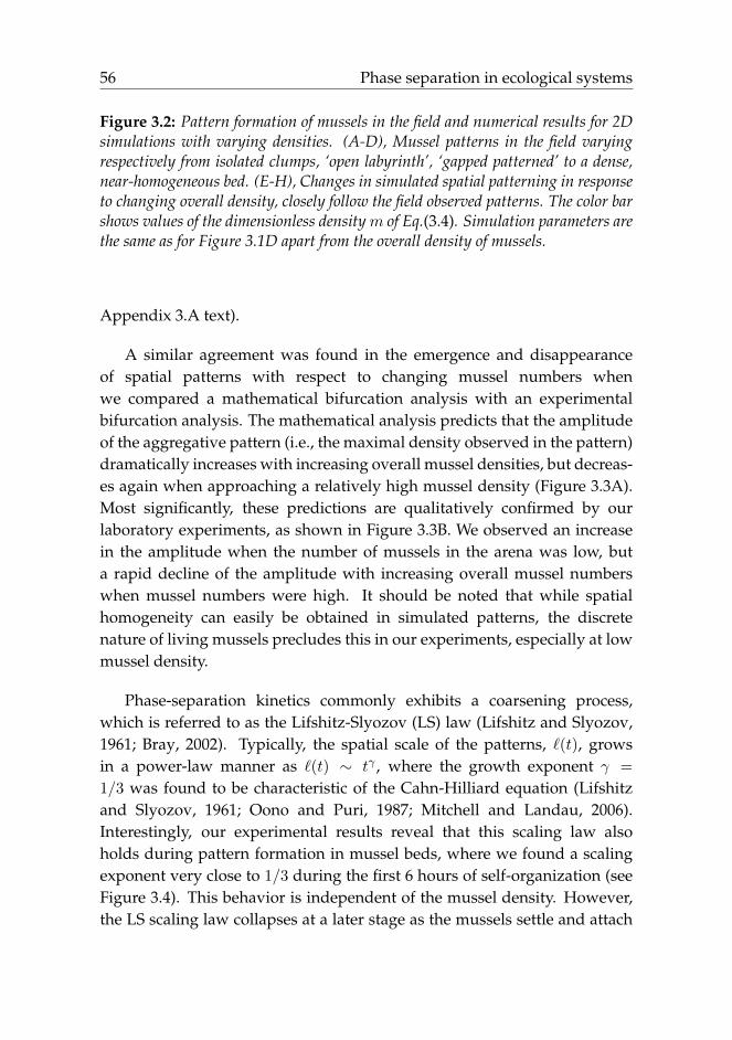
Figure 3.2: Pattern formation of mussels in the field and numerical results for 2Dsimulations with varying densities. (A-D), Mussel patterns in the field varyingrespectively from isolated clumps, ‘open labyrinth’, ‘gapped patterned’ to a dense,near-homogeneous bed. (E-H), Changes in simulated spatial patterning in responseto changing overall density, closely follow the field observed patterns. The color barshows values of the dimensionless densitym of Eq.(3.4). Simulation parameters arethe same as for Figure 3.1D apart from the overall density of mussels.
Appendix 3.A text).
A similar agreement was found in the emergence and disappearanceof spatial patterns with respect to changing mussel numbers whenwe compared a mathematical bifurcation analysis with an experimentalbifurcation analysis. The mathematical analysis predicts that the amplitudeof the aggregative pattern (i.e., the maximal density observed in the pattern)dramatically increases with increasing overall mussel densities, but decreas-es again when approaching a relatively high mussel density (Figure 3.3A).Most significantly, these predictions are qualitatively confirmed by ourlaboratory experiments, as shown in Figure 3.3B. We observed an increasein the amplitude when the number of mussels in the arena was low, buta rapid decline of the amplitude with increasing overall mussel numberswhen mussel numbers were high. It should be noted that while spatialhomogeneity can easily be obtained in simulated patterns, the discretenature of living mussels precludes this in our experiments, especially at lowmussel density.
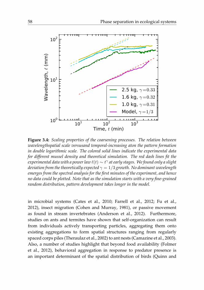
Phase-separation kinetics commonly exhibits a coarsening process,which is referred to as the Lifshitz-Slyozov (LS) law (Lifshitz and Slyozov,1961; Bray, 2002). Typically, the spatial scale of the patterns, `(t), growsin a power-law manner as `(t) ∼ tγ , where the growth exponent γ =
1/3 was found to be characteristic of the Cahn-Hilliard equation (Lifshitzand Slyozov, 1961; Oono and Puri, 1987; Mitchell and Landau, 2006).Interestingly, our experimental results reveal that this scaling law alsoholds during pattern formation in mussel beds, where we found a scalingexponent very close to 1/3 during the first 6 hours of self-organization (seeFigure 3.4). This behavior is independent of the mussel density. However,the LS scaling law collapses at a later stage as the mussels settle and attach

Chapter 3 57
0.2 0.3 0.4 0.5 0.6 0.7Mussel density
0.2
0.3
0.4
0.5
0.6
0.7A
mplit
ude a
t peak
E
F
G
H
A
050100
150
200
0.2 0.4 0.6 0.8 1.0 1.2 1.4Mussel density (cm−2 )
0.2
0.4
0.6
0.8
1.0
1.2
1.4
Am
plit
ude a
t peak
B
Figure 3.3: Bifurcation of the amplitude of patterns as a function of mussel densityas predicted by the theoretical model (A) and found in the experimental patterns(B). (A), Parameter values are β = 1.89, D0 = 1.0, and κ = 0.1, apart frommussel density; letters indicate position on the plot corresponding to the foursnapshots E, F, G and H in Figure 3.2. The mussel density represents values ofthe dimensionless density. (B), Laboratory measurement of patterned amplitudeswith different densities on surface of 30 cm by 50 cm, where the number of musselsranges from 100 to 1400 individuals. Amplitude versus the mean density is depictedas symbol lines with solid squares (�), the red lines depict average density.
to each other with byssus threads. Our theoretical model (3.4) matches thisresult displaying the same scaling exponent as our experiments (note that asthe simulation starts with a very fine-grained random distribution, patterndevelopment takes longer in the model in Figure 3.4).
Discussion
The results reported here establish a new general principle for spatialself-organization in ecological systems that is based on density-dependentmovement rather than scale-dependent activator-inhibitor feedback. Thisphase separation-based process was until now not recognized as ageneral mechanism for pattern formation in ecology, despite aggregationby individual movement being a commonly described phenomenon inbiology (Turchin, 1998; Mittal et al., 2003; Buhl et al., 2006; Liu et al., 2011;Vicsek and Zafeiris, 2012). Recent theoretical studies highlight similaraggregative processes as a possible mechanism behind pattern formation
58 Phase separation in ecological systems
101 102 103
Time, t (min)
100
101
102
Wavele
ngth
, `
(mm
)
2.5 kg, γ=0.33
1.6 kg, γ=0.32
1.0 kg, γ=0.31
Model, γ=1/3
Figure 3.4: Scaling properties of the coarsening processes. The relation betweenwavelengthspatial scale versusand temporal-increasing aton the pattern formationin double logarithmic scale. The colored solid lines indicate the experimental datafor different mussel density and theoretical simulation. The red dash lines fit theexperimental data with a power law `(t) ∼ tγ at early stages. We found only a slightdeviation from the theoretically expected γ = 1/3 growth. No dominant wavelengthemerges from the spectral analysis for the first minutes of the experiment, and henceno data could be plotted. Note that as the simulation starts with a very fine-grainedrandom distribution, pattern development takes longer in the model.
in microbial systems (Cates et al., 2010; Farrell et al., 2012; Fu et al.,2012), insect migration (Cohen and Murray, 1981), or passive movementas found in stream invertebrates (Anderson et al., 2012). Furthermore,studies on ants and termites have shown that self-organization can resultfrom individuals actively transporting particles, aggregating them ontoexisting aggregations to form spatial structures ranging from regularlyspaced corps piles (Theraulaz et al., 2002) to ant nests (Camazine et al., 2003).Also, a number of studies highlight that beyond food availability (Folmeret al., 2012), behavioral aggregation in response to predator presence isan important determinant of the spatial distribution of birds (Quinn and

Chapter 3 59
Cresswell, 2006). These studies indicate there may be a wide potential forapplication of the Cahn-Hilliard framework of phase separation in ecologyand animal behavior that extends well beyond our mussel case study.
A fundamental difference exists between pattern formation as predictedby Turing’s activator-inhibitor principle and that predicted by Cahn-Hilliard principle for phase separation. Characteristic of Turing patternsis that a homogeneous ‘background state’ becomes unstable with respectto small spatially periodic perturbations: this so-called Turing instability isthe driving mechanism behind the generation of spatially periodic Turingpatterns. Moreover, the fixed wavelength of these patterns is determinedby this instability. In the Cahn-Hilliard equation there is no such ‘unstablebackground state’ that can be seen as the core from which patterns grow.Moreover, there is no specific wavelength that defines the pattern. Rather,the Cahn-Hilliard equation exhibits a coarsening process: the wavelengthslowly grows in time. Hence, Cahn-Hilliard dynamics have the nature ofbeing forced to interpolate between two stable states, or phases, while aTuring instability is ‘driven away from an unstable state’.
Strikingly, in mussels, both processes may occur at the same time. Mus-sels aggregate because they experience lower mortality due to dislodgementor predation in clumps (van de Koppel et al., 2008). This explains why on theshort term, they aggregate in a process that, as we argue in this paper, can bedescribed by Cahn and Hilliard’s model for phase separation. On the longterm, however, they settle and attach to other mussels using byssal threads,a process that arrests pattern formation, thereby disabling the coarseningnature of ‘pure’ Cahn-Hilliard dynamics by a biological mechanism thatacts on intermediate time scales and has not been taken into account in thepresent model that focuses on the first 24 hours of the process. Moreover, atan even longer time scale, mortality and individual growth further shapesthe spatial structure of mussel beds, unless a disturbance leads to large-scaledislodgement, which is likely to reinitiate aggregative movement. Hence,on the long run, both demographic processes (van de Koppel et al., 2005)and aggregative movement (van de Koppel et al., 2008) shape the patternsthat are observed in real mussel beds.
Finally, our results demonstrate that to understand complexity inecological systems, we need to recognize the importance of movement as a
60 Phase separation in ecological systems
process that can create coherent spatial structure in ecosystems, rather thanjust dissipate them. Unlike the growth/mortality based Turing mechanism,the movement-based Cahn-Hilliard mechanism has short time scales. Itmay thus allow for fast adaptation and generate transient spatial structuresin ecosystems. In natural ecosystems, both processes occur, sometimeseven within the same ecosystems. How the interplay between these twomechanisms affects the complexity and resilience of natural ecosystems isan important topic for future research.
Chapter 3 61
Appendix 3.A: Materials and Methods
Laboratory setup and mussel sampling
The laboratory setup followed that of a previous study by van de Koppelet al. (2008). Pattern formation by mussels was studied in the laboratorywithin a 130 cm by 90 cm by 27 cm polyester container filled with seawater.Mussel samples were obtained from wooden wave-breaker poles on thebeaches near Vlissingen, the Netherlands (51.458713◦N, 3.531643◦E). Theywere kept in containers and fed live cultures of Phaeodactylum tricornutumdaily. In the experiments, mussels were laid-out evenly on a surface ofeither concrete tiles or a red PVC sheet. The container was illuminated usingfluorescent lamps. Fresh, unfiltered seawater was supplied to the containerat a rate of approximately one liter per minute.
Imaging procedures and mussels’ tracking
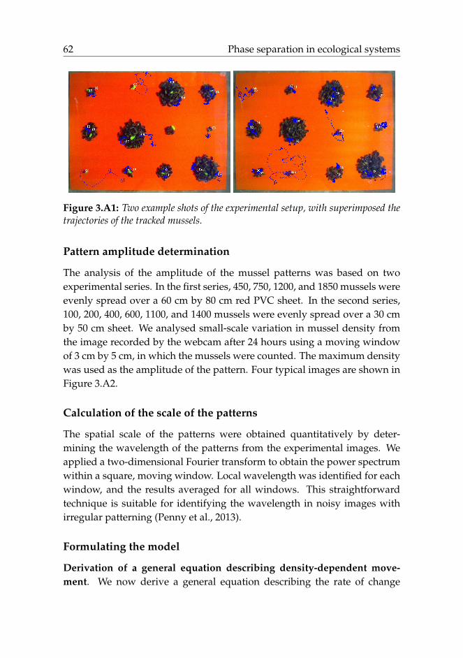
The movement of individual mussels was recorded by taking an imageevery minute using a Canon PowerShot D10, which was positioned about60 cm above the water surface, and attached to a laptop computer. Eachimage contained the entire experimental domain at a 3000 by 4000 pixelsresolution. We tested the effect of increasing mussel densities on movementspeed. We set up a series of mussel clusters with 1, 2, 4, 6, 8, 16, 24, 32,64, 80, 104, and 128 mussels respectively on a red PVC sheet to providea contrast-rich surface for later analysis (see Figure 3.A1). The movementspeed of individual mussels was obtained by measuring the movementdistance along the trajectories during one minute. All image analysis andtracking programs are developed in Matlab (R2012a, c© The Mathworks,Inc) (www.mathworks.com).
Field photos of mussel patterns
Field photos of mussel patterns with different densities were taken on thetidal flats opposite to Gallows Point (53.245238◦N, -4.104166◦E) near MenaiBridge, UK, in July 2006.
62 Phase separation in ecological systems
Figure 3.A1: Two example shots of the experimental setup, with superimposed thetrajectories of the tracked mussels.
Pattern amplitude determination
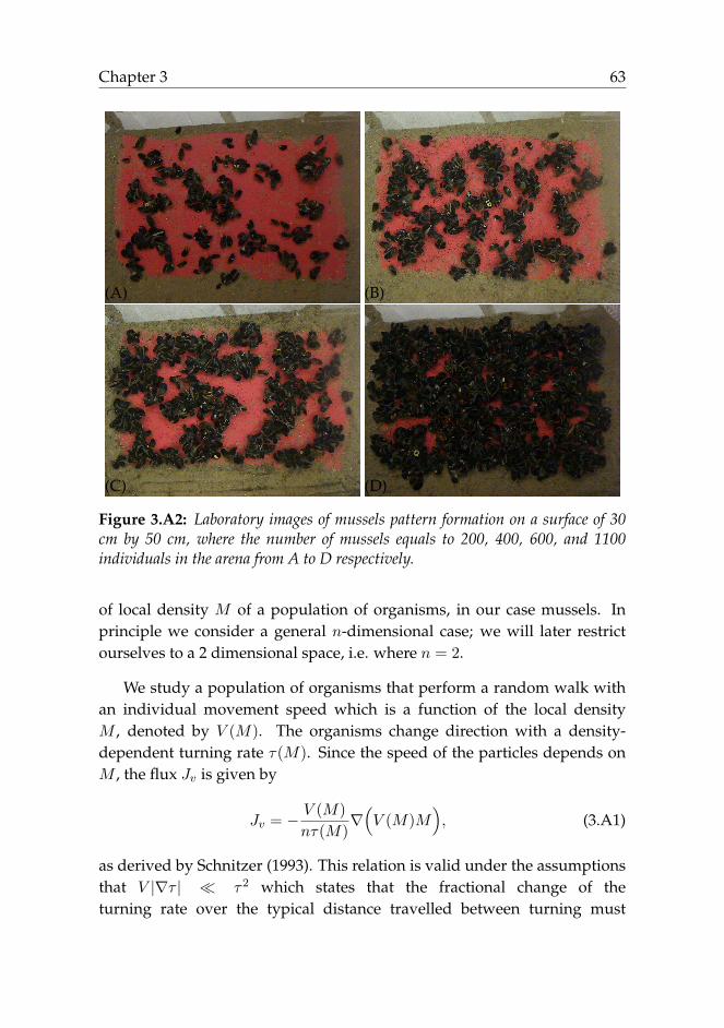
The analysis of the amplitude of the mussel patterns was based on twoexperimental series. In the first series, 450, 750, 1200, and 1850 mussels wereevenly spread over a 60 cm by 80 cm red PVC sheet. In the second series,100, 200, 400, 600, 1100, and 1400 mussels were evenly spread over a 30 cmby 50 cm sheet. We analysed small-scale variation in mussel density fromthe image recorded by the webcam after 24 hours using a moving windowof 3 cm by 5 cm, in which the mussels were counted. The maximum densitywas used as the amplitude of the pattern. Four typical images are shown inFigure 3.A2.
Calculation of the scale of the patterns
The spatial scale of the patterns were obtained quantitatively by deter-mining the wavelength of the patterns from the experimental images. Weapplied a two-dimensional Fourier transform to obtain the power spectrumwithin a square, moving window. Local wavelength was identified for eachwindow, and the results averaged for all windows. This straightforwardtechnique is suitable for identifying the wavelength in noisy images withirregular patterning (Penny et al., 2013).
Formulating the model
Derivation of a general equation describing density-dependent move-ment. We now derive a general equation describing the rate of change
Chapter 3 63
(A) (B)
(C) (D)
Figure 3.A2: Laboratory images of mussels pattern formation on a surface of 30cm by 50 cm, where the number of mussels equals to 200, 400, 600, and 1100individuals in the arena from A to D respectively.
of local density M of a population of organisms, in our case mussels. Inprinciple we consider a general n-dimensional case; we will later restrictourselves to a 2 dimensional space, i.e. where n = 2.
We study a population of organisms that perform a random walk withan individual movement speed which is a function of the local densityM , denoted by V (M). The organisms change direction with a density-dependent turning rate τ(M). Since the speed of the particles depends onM , the flux Jv is given by
Jv = − V (M)
nτ(M)∇(V (M)M
), (3.A1)
as derived by Schnitzer (1993). This relation is valid under the assumptionsthat V |∇τ | � τ2 which states that the fractional change of theturning rate over the typical distance travelled between turning must

64 Phase separation in ecological systems
be small (Schnitzer, 1993). We also incorporate the effect of non-localmovement in the model which results in a second contribution to theflux (Murray, 2002, see p.408-416 for details),
Jnl = κ∇(∆M), (3.A2)
for some constant κ > 0 (here ∆ = ∇2). See literature (Cates et al., 2010;Murray, 2002) for a similar approach.
We study the population on relatively short time-scales of maximallyone day, at which birth and mortality processes play a relatively minor role.For this reason, we do not consider demographic processes in our modelanalysis. Combining the above assumptions, changes in the local density oforganisms can be described by
∂M
∂t= −∇(Jv + Jnl),
in which M is - by construction - a conserved quantity. Combining (3.A1)and (3.A2), leads to
∂M
∂t= ∇ [f(M)∇M − κ∇∆M ] , (3.A3)
where f(M) = V2τ
(V +M ∂V
∂M
), and V and τ are, in general, functions of M .
For simplicity, we consider the turning rate τ to be independent of M .Moreover, we restrict the problem to two dimensions, and hence n = 2.Note that since V is the speed of the organisms in the population, V (M) > 0,for all M and since f(M) = V
2τ (V +M ∂V∂M ), the occurrence of zeros in f(M)
is controlled by V +M ∂V∂M , and thus by the parameters in V .
The derivation of the mussel movement model (3.4). Based on the dataobtained from the experiments and the analysis provided in the main text,we assume a parabolic relation between speed V and density M :
V (M) = aM2 − bM + c,
where the values of the constants a, b, c can be obtained from theexperimental data.
Chapter 3 65
With this definition of V , we can derive function f(M):
f(M) =1
2τ(aM2 − bM + c)(3aM2 − 2bM + c),
so that by introducing m =√
acM and β = b√
ac, (3.A3) can be written as
∂m
∂t= D0∇ [g(m)∇m− κ1∇ ·∆m] , (3.A4)
where g(m) =(m2 − βm+ 1
) (3m2 − 2βm+ 1
), with D0 = c2
2τ , κ1 = 2τκc2
,and β2 < 4 (since V (m) > 0).
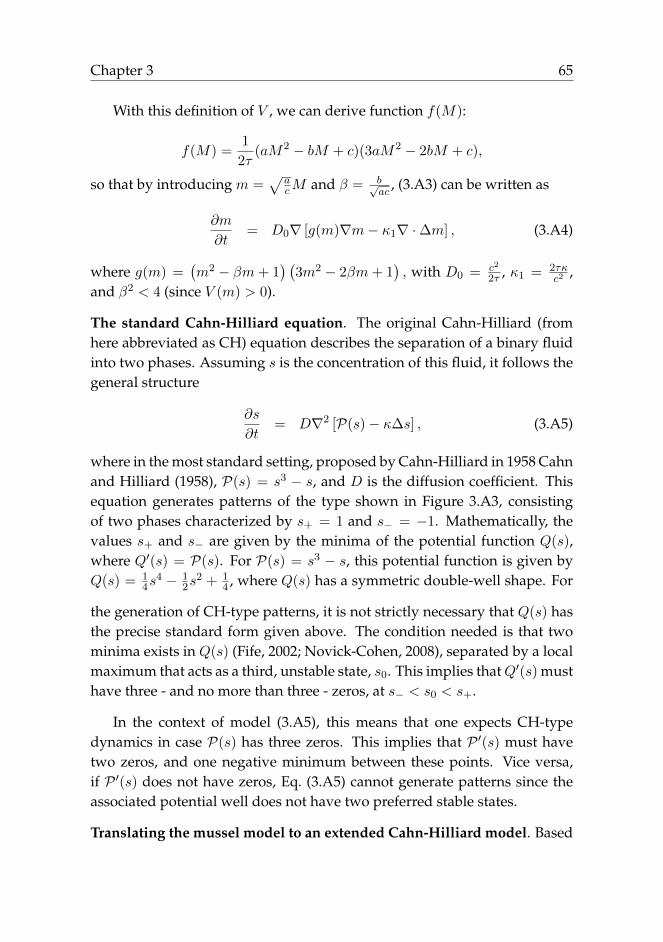
The standard Cahn-Hilliard equation. The original Cahn-Hilliard (fromhere abbreviated as CH) equation describes the separation of a binary fluidinto two phases. Assuming s is the concentration of this fluid, it follows thegeneral structure
∂s
∂t= D∇2 [P(s)− κ∆s] , (3.A5)
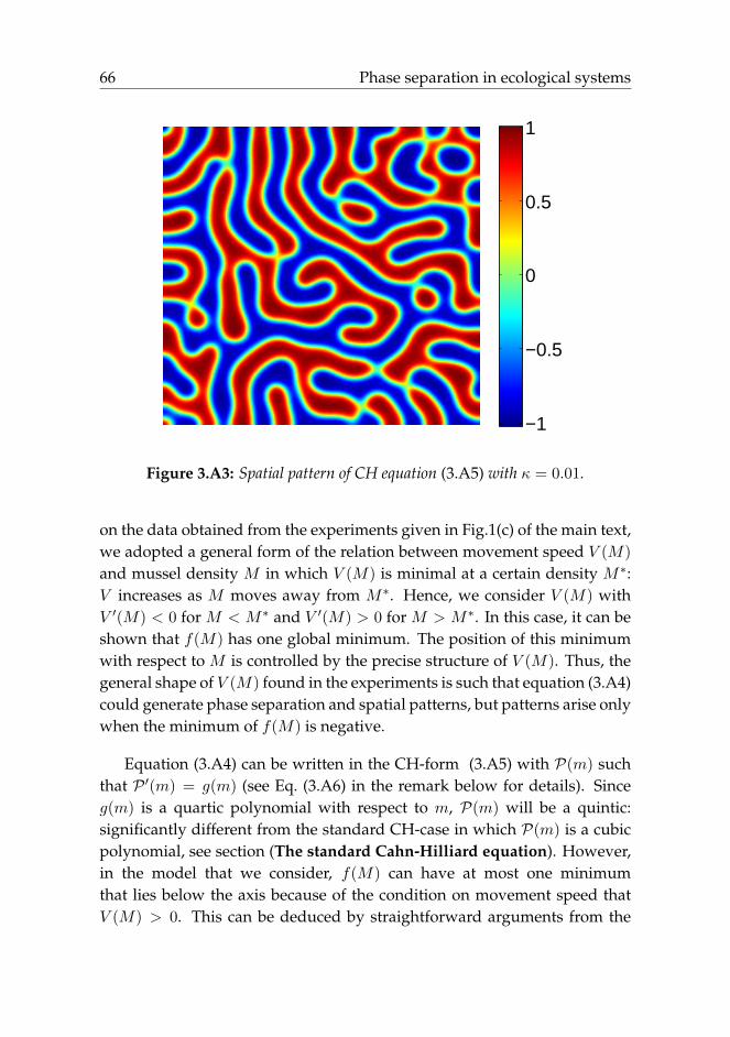
where in the most standard setting, proposed by Cahn-Hilliard in 1958 Cahnand Hilliard (1958), P(s) = s3 − s, and D is the diffusion coefficient. Thisequation generates patterns of the type shown in Figure 3.A3, consistingof two phases characterized by s+ = 1 and s− = −1. Mathematically, thevalues s+ and s− are given by the minima of the potential function Q(s),where Q′(s) = P(s). For P(s) = s3 − s, this potential function is given byQ(s) = 1
4s4 − 1
2s2 + 1
4 , where Q(s) has a symmetric double-well shape. For
the generation of CH-type patterns, it is not strictly necessary that Q(s) hasthe precise standard form given above. The condition needed is that twominima exists in Q(s) (Fife, 2002; Novick-Cohen, 2008), separated by a localmaximum that acts as a third, unstable state, s0. This implies thatQ′(s) musthave three - and no more than three - zeros, at s− < s0 < s+.
In the context of model (3.A5), this means that one expects CH-typedynamics in case P(s) has three zeros. This implies that P ′(s) must havetwo zeros, and one negative minimum between these points. Vice versa,if P ′(s) does not have zeros, Eq. (3.A5) cannot generate patterns since theassociated potential well does not have two preferred stable states.
Translating the mussel model to an extended Cahn-Hilliard model. Based
66 Phase separation in ecological systems
−1
−0.5
0
0.5
1
Figure 3.A3: Spatial pattern of CH equation (3.A5) with κ = 0.01.
on the data obtained from the experiments given in Fig.1(c) of the main text,we adopted a general form of the relation between movement speed V (M)
and mussel density M in which V (M) is minimal at a certain density M∗:V increases as M moves away from M∗. Hence, we consider V (M) withV ′(M) < 0 for M < M∗ and V ′(M) > 0 for M > M∗. In this case, it can beshown that f(M) has one global minimum. The position of this minimumwith respect to M is controlled by the precise structure of V (M). Thus, thegeneral shape of V (M) found in the experiments is such that equation (3.A4)could generate phase separation and spatial patterns, but patterns arise onlywhen the minimum of f(M) is negative.
Equation (3.A4) can be written in the CH-form (3.A5) with P(m) suchthat P ′(m) = g(m) (see Eq. (3.A6) in the remark below for details). Sinceg(m) is a quartic polynomial with respect to m, P(m) will be a quintic:significantly different from the standard CH-case in which P(m) is a cubicpolynomial, see section (The standard Cahn-Hilliard equation). However,in the model that we consider, f(M) can have at most one minimumthat lies below the axis because of the condition on movement speed thatV (M) > 0. This can be deduced by straightforward arguments from the

Chapter 3 67
observational fact that V (M) only has one minimum at M = M∗ (anddecreases, respectively increases, for M < M∗, resp. M > M∗). Thus, inthe present model only CH-type patterns may develop. This is also typicalbehavior if we drop the assumption that the turning rate τ is constant, andtake it to depend on the mussel concentration M . Since the turning ratemust remain positive for all M , it is not possible to create additional zeroesin f(M) by varying τ . Hence, also in this more general case, the dynamicsgenerated by (3.A3) remain of CH-type.
It is straightforward to ‘control’ the appearance of zeros of g(m): g(m) >
0 for all m when β <√
3. As β crosses through√
3, two zeros appear: thus,CH-like patterns will appear as β2 increases through 3. This is confirmed byour simulations in the bifurcation analysis in Figure 3.A4 and the simulatedpattern in Fig.1(d).
1.7 1.8 1.9 2.0
0.4
0.6
0.8
1.0βc =
√3
Preferred
stablestates,M
Aggregation, β
Figure 3.A4: Bifurcation diagram of equation (5.4).
Remark We can easily obtain the exact expression of the CH-formula of musselmodel (3.A4) as
∂m
∂t= D0∇2 [P(m)− κ1∆m] , (3.A6)
with P(m) = 3m5
5 −5βm4
4 + (4+2β2)m3
3 − 3βm2
2 +m+H. Here,H ∈ R is a new

68 Phase separation in ecological systems
parameter.
Numerical implementation
The continuum equation (3.A4) was simulated on a HP Z800 workstationwith an NVidia Tesla C1060 graphics processor. For the two-dimensionalspatial patterns, our computation code was implemented in the CUDAextension of the C language (www.nvidia.com/cuda). The spatial fourth-order kernel is implemented in two-dimensional space using the numericalschemes shown in Figure 3.A5. Spatial patterns were obtained by Eulerintegration of the finite-difference equation with discretization of thediffusion van de Koppel et al. (2011). The model’s predictions wereexamined for different grid sizes and physical lengths. We adopted periodicboundary conditions for the rectangular spatial grid. Starting conditionsconsisted of a homogeneous distribution of mussels with a slight randomperturbation. All results were obtained by setting ∆t = 0.001 and ∆x =
0.15.
1 -4 6 -4 1
1
2 -8 2
1 -8 20 -8 1
2 -8 2
1
Figure 3.A5: The kernel∇4 in two-dimensional space.
Correlations analysis
The comparison of images obtained from the mussel beds on the tidal flatsnear Menai Bridge with results of the numerical solution of model (3.A4)

Chapter 3 69
reveals a remarkable similarity of the real mussel beds with the modelprediction (see Fig. 2 in main text). Of course, due to the inherentstochastic nature of the real mussel ecological system, the snapshots donot match precisely. To reach a quantitative assessment on the validity ofthe model (3.A4) to describe the spatial properties of the mussel system inthe short-time scale, we have computed spatial correlation function for thesystem’s spatial patterns.
We consider equal-time spatial correlation functions (in fact, thesystem displays coarsening at long-time scale, then we must choose theappropriate timescale), which yield information about the size of theemerging patterns. Here, we focus on the correlation function, whereG(r) = 〈m(r+r′)m(r)〉−〈m(r,t)〉2
〈m(r,t)2〉−〈m(r,t)〉2 , which expressed how the value at positionm(r, t) is related to data points at some distance r′ (Arfken and Weber,2005). The spatial correlation function, G(r), averaged for specie distanceclasses over the entire density field, reveals the global behavior of thepattern as a function of spatial scale. The position of the first peak gives themean wavelength of spatial patterns. In Figure 3.A6, we show the spatialcorrelation function obtained for both field patterns and from the predictedpatterns of model (3.A4), after a timescale of about 24 hours, revealing anexcellent agreement.
0 5 10 15 20 25 30distance, r (cm)
0.2
0.0
0.2
0.4
0.6
0.8
1.0
Corr
ela
tion f
unct
ion
Experiment
Simulation
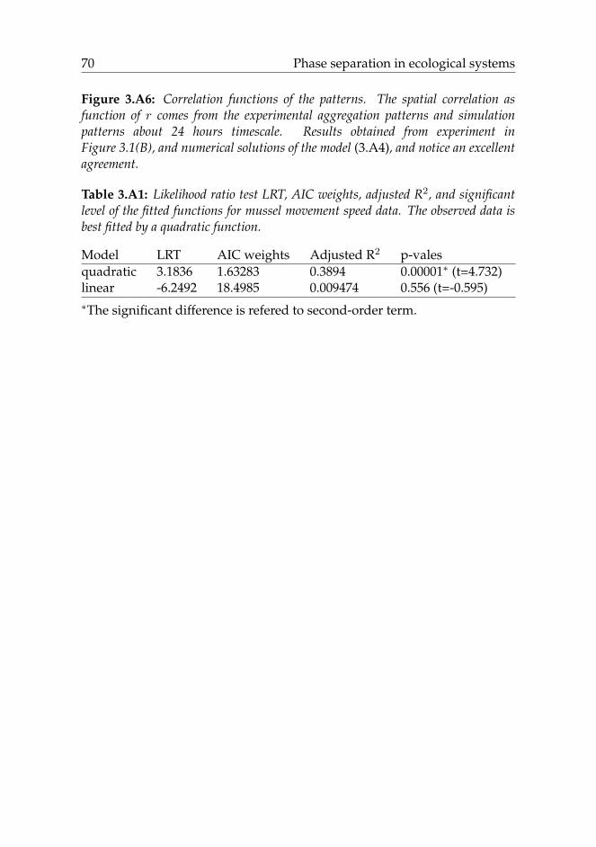
70 Phase separation in ecological systems
Figure 3.A6: Correlation functions of the patterns. The spatial correlation asfunction of r comes from the experimental aggregation patterns and simulationpatterns about 24 hours timescale. Results obtained from experiment inFigure 3.1(B), and numerical solutions of the model (3.A4), and notice an excellentagreement.
Table 3.A1: Likelihood ratio test LRT, AIC weights, adjusted R2, and significantlevel of the fitted functions for mussel movement speed data. The observed data isbest fitted by a quadratic function.
Model LRT AIC weights Adjusted R2 p-valesquadratic 3.1836 1.63283 0.3894 0.00001∗ (t=4.732)linear -6.2492 18.4985 0.009474 0.556 (t=-0.595)∗The significant difference is refered to second-order term.