1

The effects of variation in management objectives on responses to

forest diseases under uncertainty

C.E. Dangerfielda, A.E. Whalleyb, N. Hanleyc, J.R. Healeyd and C.A. Gilligana

a Department of Plant Sciences, University of Cambridge, Downing Street, Cambridge, CB2 3EA, UK b Warwick Business School, The University of Warwick, Coventry, CV4 7AL, UK c School of Geography & Geosciences, Irvine Building, University of St Andrews, North Street, St Andrews, Fife, KY16 9AL, UK d School of Environment, Natural Resources & Geography, Thoday Building, University of Bangor, Deiniol Road, Bangor, Gwynedd, LL57 2UW, UK

Abstract

The real options approach provides a powerful tool for determining the optimal time at which

to adopt disease control measures given that there is uncertainty about the future spread of an

invading pest or pathogen. Previous studies have considered the timing of control from the

point of view of a central planner. However, decisions regarding the deployment of control

measures are typically taken by individual forest managers, who may have widely differing

objectives. In this article we investigate how management objectives impact the optimal

timing of control measures given uncertainty in disease spread. Our results show that

differences in management objectives can lead managers to act at different times, and

potentially never adopt disease control. In particular, these differences in the timing of

disease control for diverse types of managers become more significant if the disease impacts

the range of benefits from the forest to varying extents. This creates tensions at the landscape

scale if there are managers with divergent objectives due to the transferable externality (the

disease). Targeted subsidies which lower the ongoing costs of control can reduce differences

in control strategies between managers with divergent objectives. Our results have important

implications for national decision making bodies and suggest that incentives may need to be

targeted at specific groups to ensure a coherent response to disease control.

We thank the BBSRC for funding this work under the Tree Health and Plant

Biosecurity Initiative.

2

There has been a significant rise in invasive pathogens and pests within forests in recent

years, and the problem is set to worsen in the future, largely due to climate change and

changing trade patterns (Hanley and MacPherson 2016; Sturrock et al. 2011; Freer-Smith and

Webber 2015). Such pathogens and pests can cause significant damage (often mortality) to

trees leading to negative economic and ecological impacts on forests and so pose an

important threat to the British forestry industry, and to public goods such as recreation and

biodiversity conservation that forests provide.

When a new pest or pathogen1 arrives, a key choice facing a forest owner is whether or not to

adopt control measures to reduce the spread of the pest or pathogen. The owner must weigh

up the costs of control against the potential reduction to the benefits of their forest as a result

of pest or pathogen damage. However, these future benefits are uncertain due to the

uncertainty in the future progression of the pest or pathogen as a result of environmental

fluctuations such as climatic conditions, evolution within the pathogen species, and scientific

uncertainty about how the disease is transmitted and about the effectiveness of treatment

options. Furthermore, owners differ in the benefits they obtain from the forest depending on

their given objectives. So while it may be in one owner’s interest to adopt control, the same is

not necessarily true for another owner with different objectives for their forest. A key aim of

this article it to bring these two elements together so as to investigate how the interaction

between future uncertainty in disease spread and forest management objectives affect when

(if ever) it is optimal for an individual forest manager to adopt control measures to mitigate

damage due to invasive pathogens or pests.

Our findings suggest there can be significant variation in the timing of pest or pathogen

control measures between forests managed under different management objectives. This can

create tensions at the landscape scale due to the transferable externality (the disease) which

1 We use the terms ‘disease’ and ‘pest or pathogen’ interchangeably; see Section 2 for further discussion.

3

does not respect land ownership boundaries. We thus further investigate the impact of

subsidies on control strategies and the extent to which targeted subsidies can reduce the

divergence in these strategies between forests managed with different objectives. We find

that subsidies which reduce ongoing costs of control both bring forward the initial adoption

of control and delay any subsequent cancellation of control measures, whereas subsidies

which reduce control initiation costs bring forward not only initial adoption but also

subsequent cancellation of control measures. These results rely on the dynamic nature of our

epidemiologically-based real options modelling framework, which allows for both adoption

and cancellation of control measures as the impact of pests or pathogens varies over time.

A major economic challenge in controlling invasive pests and pathogens is that such

measures involve both sunk and on-going costs. Sunk costs represent irreversible losses to

the land manager. This, combined with the uncertainty in the future progress of disease

means there can be value in waiting to learn more before initiating costly control measures (J

Saphores 2000; Sims and Finnoff 2012; Sims and Finnoff 2013; Ndeffo Mbah et al. 2010;

Marten and Moore 2011). Previous studies have shown this using a real options approach,

since it provides a powerful way to analyse the joint effects of uncertainty and learning, in the

context of irreversibility. By viewing disease control as an option that can be exercised to

reduce damage by a pest or pathogen to the host species, the real options approach provides a

threshold in the proportion of infected area at which it is optimal to deploy control

immediately.

Saphores (2000) first applied the real options approach to determine the impact of uncertainty

in future area infected by a pest on the optimal timing of pesticide application. Varying the

level of uncertainty, Saphores (2000) showed that greater uncertainty in future infected area

increases the threshold at which it is optimal to spray. This gives rise to the “wait-and-see”

approach to dealing with invasive pests or pathogens: when there is uncertainty in the future

4

dynamics of area infected by a pest or pathogen, there is value in waiting to learn more before

investing in control. Saphores (2000) assumes that the application of pesticide is irreversible,

that is once pesticide application is initiated it can never be cancelled. However, in reality this

is usually not the case since such measures are on-going and can be stopped at any time.

Indeed, Sims et al. (2016) argue that the only example of a truly irreversible control measure,

i.e. one that cannot be stopped at some point in the future once it has been initiated, is the

release of a biological control agent. Sims & Finnoff (2013) consider the implications of the

reversibility of the control measure on how long a regulator should wait to take action. They

find that if control measures are partly reversible (for example trade bans), then it is optimal

to act earlier than if measures are completely irreversible. This shows that how long it is

optimal to “wait and see” depends not only on the future uncertainty in infected area but also

on the nature of actions which can be taken, i.e. how reversible the control measures are.

Traditionally, the uncertainty in the spread of the pest or pathogen is assumed to follow a

Geometric Brownian Motion (GBM) (Saphores 2000). The advantage of such an assumption

is that GBM is well understood and allows for closed-form solutions to the real options

problem. However, GBM is unbounded above and so it does not respect the upper boundary

in the infected area which arises due to the limited number of available hosts within a given

spatial domain. Sims & Finnoff (2012) consider the impact of introducing a spatial boundary

on the timing of control, by incorporating an exogenous upper boundary into the decision

problem. This is to prevent the threshold at which control occurs rising above the maximum

area that can be infected. They find that spatial scale can affect the timing and stringency of

control strategies, and so incorporating an upper bound is important in planning measures to

minimise losses from pest or pathogen damage (Sims and Finnoff 2012).

Other authors have tried to incorporate the limiting nature of pest or pathogen spread by

adapting the stochastic processes used to describe the uncertainty in future infected area.

5

Ndeffo Mbah et al. (2010) incorporate a logistic-type term into the drift coefficient of the

stochastic differential equation (SDE) describing the increase in area infected by the pest or

pathogen, so the mean growth of the process is limited by a parameter that represents the

maximum area that can be infected. They find that the new SDE leads to qualitatively

different behaviour in the relationship between the optimal timing of control adoption and

uncertainty. While the SDE used by Ndeffo Mbah et al. (2010) more realistically captures the

logistic nature of growth in area infected by the pest or pathogen, such a process does not

respect the upper boundary in infected area. Dangerfield et al. (2016) show that incorporating

a logistic-type term into both the drift and diffusion coefficients of the SDE describing

growth in infected area ensures that the upper boundary is endogenously incorporated into the

decision problem. Formulating the dynamics using this epidemiologically-based stochastic

process leads to control being deployed earlier, which has important implications for decision

makers such as forest managers or government agencies.

In previous studies, the optimal timing of control is typically considered from the point of

view of a central planner (Sims and Finnoff 2013; Sims and Finnoff 2012; Marten and Moore

2011). However, since areas of forest can be privately owned, for example in Britain it is

estimated that around 70% of forests are privately owned (Fitter 1980), whether or not to

adopt control measures will be decided by the individual owners, rather than a central

planner. Furthermore, the way in which an owner manages their forest will depend on a

specific set of forestry objectives, which can vary significantly between different owners.

Urquhart & Courtney (2011) identified six distinct groups of forest owners in England based

on common objectives, motivations and attitudes within each group. For example, Urquhart

& Courtney (2011) defined the ‘investor’ group as those who prioritise timber production and

investment opportunities in their forestry objectives, and do not manage their forests for non-

timber benefits such as wildlife conservation or recreation. On the other hand, the

6

‘conservationist’ group were motivated to manage their forests to conserve biodiversity and

do not consider timber production as a significant output (Urquhart and Courtney 2011). This

heterogeneity in the priorities of different forest owners means they place different

weightings on the individual benefits obtained from the forest. Combined with this is the fact

that pests and pathogens do not affect the different benefits arising from the forest uniformly,

and so there is inconsistency in the level of effect a given pest or pathogen has on a particular

benefit. For example, dothistroma needle blight causes premature needle loss on pine trees,

which leads to significant reductions in tree growth and so can result in substantial losses in

timber value over a rotation period2. On the other hand, this reduction in growth has a lower

impact on biodiversity and amenity value. In such situations there is less of an incentive for

an owner within the conservationist group to control against the pathogen or pest as

compared with an investor whose priority is timber production. Differences in the objective

function explicitly or implicitly used by each forest owner are therefore likely to affect how

they respond to a particular pest or pathogen risk, and thus how that pest or pathogen spreads

across a landscape.

In this article we investigate how the objectives of a forest owner affect how long they will

optimally wait before adopting a control measure, given that there is uncertainty over the

future progress of the pest or pathogen. Using a real options approach to incorporate

uncertainty into the decision process, we explore how varying the function that describes the

value of the forest (the owner’s objective function) influences the threshold at which control

should be adopted immediately. This provides insight into how variations in the different

benefits obtained from a forest will affect an individual forest owner’s optimal time to

control. These benefits could reflect the value which a forest owner gets from both timber and

non-timber attributes, and/or a Payment for Ecosystem Services which they receive for

2 http://www.forestry.gov.uk/pdf/fcrn002.pdf/$FILE/fcrn002.pdf

7

producing public good-type benefits along with the financial benefits of timber production.

We model the forest owner as taking decisions over control measures in their forest

independently of other forest owners, in the sense that expectations over the actions of others

do not enter into their decision-making process.

We find that while the heterogeneity in forest management objectives leads to differences in

the region of infected area at which control should be adopted, these differences are small

when the pest or pathogen affects the timber and non-timber benefits of the forest in a

uniform way. Therefore, our results suggest that the diversity in forest management

objectives alone does not lead to significant variation in the timing of pest or pahtogen

control measures between different managers. On the other-hand when the heterogeneity of

management objectives is combined with differences in the reduction of timber and non-

timber benefits then the discrepancies between the control strategies of dissimilar managers

becomes more significant. Indeed it may be optimal for one manager never to adopt control,

while the other should adopt control as soon as the proportion of infected area exceeds some

threshold level. In such situations, we show that the discrepancy in the control strategies of

different managers can be reduced through subsidy schemes that reduce the costs of control.

We consider two types of subsidy: the first reduces the one-off cost of initiating disease

control, whereas the second instead reduces the ongoing costs of control. We find that, while

both types of subsidy increase the range of proportions of infected area for which control is

adopted, subsidies which reduce ongoing costs of control are more effective in expanding the

region where control continues to be applied.

Our results have important implications for local and national decision making bodies, such

as the UK Government Department for Environment Food and Rural Affairs (DEFRA), the

Forestry Commission in England and Scotland and Natural Resources Wales, who seek to

achieve reductions in pest or pathogen spread at a larger spatial scale than an individual

8

forest. Our results identify the combinations of disease characteristics for which disease

control strategies are likely to differ significantly for forests managed according to different

objectives, indicate how subsidies affect these disease control strategies and hence suggest

which form of subsidies (lump-sum or ongoing) are more likely to be effective in increasing

the long-term incidence of disease control. The structure of the remainder of the paper is as

follows. Section 2 introduces the model, Section 3 presents the results, and Section 4

concludes.

2. Method

In this article, we use terminology typically associated with an invasive pathogen rather than

pest, and so we refer to trees as being infected or diseased, rather than invaded. This is for

ease of writing, but we note that the model frameworks described here apply equally well to

invasive pests, such as oak processionary moth and oriental gall wasp, two pests that have

been found in England in recent years.

2.1 Value of the Forest in the Absence of Disease

Consider an area of even-aged forest composed of a single species that is of size L hectares.

We assume the value of the forest after a fixed period of time T years, where T is an

exogenous time that could, for example, represent the length of a pre-determined rotation

period, to be composed of two parts: a single payment that is received at the final time T,

which represents the net return from selling the timber, 𝑀(𝐿) , and an annual payment that

characterises the value obtained from a flow of non-timber benefits, 𝑆(𝐿). These non-timber

benefits could for example describe amenity, recreation or biodiversity values for which

either (i) the owner derives utility or (ii) for which they obtain a payment from a third party

9

such as the government. Therefore, the present value of benefits from the forest, in the

absence of disease, is given by the following equation,

𝑉𝐷𝐹(𝑇) = 𝑀(𝐿)𝑒−𝑟𝑇 + ∫ 𝑆(𝐿)

𝑇

0

𝑒−𝑟𝑡𝑑𝑡, (1)

where 𝑟 is the discount rate.

We assume that functions 𝑀(𝐿) and 𝑆(𝐿) take the following forms,

𝑀(𝐿) = 𝑝𝐿 (2)

𝑆(𝐿) = 𝑏𝐿 (3)

where p is the net return per hectare from timber sold at the end of the rotation and b is the

value per hectare of annual non-timber benefits.

2.2 Value of Forest in the Presence of Disease

Consider the outbreak of a disease within the forest of interest. We assume that the future

progress of area infected is uncertain due to the variability in infection transmission as a

result of external factors such as climatic conditions. Therefore, the proportion of area

infected over time (𝐼) changes according to the following stochastic differential equation

SDE, which we term the logistic SDE, (Dangerfield et al. 2016),

𝑑𝐼 = 𝛽𝐼(1 − 𝐼)𝑑𝑡 + 𝜎𝐼(1 − 𝐼)𝑑𝑊, (4)

where 𝛽 is the transmission rate and 𝜎 is the level of uncertainty. Since the noise term (given

by the second term in equation (4)) represents the fluctuations in the transmission parameter

𝛽 due to external factors, we assume that 𝜎 scales with 𝛽 and so 𝜎 = 𝛽 × 𝐹. The constant 𝐹

measures the magnitude of the fluctuations associated with the transmission parameter 𝛽

(Keeling and Rohani 2008). Formulating the uncertainty parameter in this way ensures that

when the transmission rate falls to 0 (i.e. when there is no transmission), the uncertainty in

10

disease spread also falls to 0. We describe the future evolution of the infected area using the

logistic SDE rather than GBM which is typically used in the literature (J Saphores 2000;

Sims and Finnoff 2013), because the logistic SDE better captures key epidemiological

features of disease spread and so ensures applicability of our results to real-world epidemics

(Dangerfield et al. 2016).

We assume that both the timber and non-timber benefits from the forest are reduced by

disease, and so infected timber value is decreased by a factor 0≤ 𝜌 ≤ 1 (e.g. because of

lower timber volume as a result of reduction in tree growth rate) and similarly annual non-

timber benefits from infected trees are lowered by a factor 0 ≤ 𝜑 ≤ 1. We assume that 𝜌 and

𝜑 are independent and consider the impact of a range of different combinations of 𝜌 and 𝜑 on

the optimal timing of control. The value of the forest, per hectare, in the presence of disease

is given by

𝑉𝐷(𝐼, 𝑇) × 𝐿 = 𝐸 [𝑝 𝐿 (1 + (𝜌 − 1)𝐼(𝑇))𝑒−𝑟𝑇

+ 𝐿 ∫ 𝑏(1 + (𝜑 − 1)𝐼(𝑡))𝑇

0

𝑒−𝑟𝑡𝑑𝑡]

(5)

where 𝐼(𝑡) is the proportion of the forest area (𝐿) that is infected at time 𝑡. Note that this is

the expected value of the forest (𝐸 in equation (5) represents the expectation), since the future

forest value is stochastic, due to the uncertainty in the future level of infection.

2.3 Optimal Timing of Disease Control

Consider a control policy that reduces the rate at which the disease spreads by a factor 0 ≤

ω ≤ 1, so the transmission rate after a control option is implemented is 𝛽𝐴 = 𝛽 × 𝜔. Since

the volatility (𝜎) is a function of 𝛽, the volatility will also be reduced after the initiation of

control measures, that is 𝜎𝐴 = 𝛽𝐴 × 𝐹. Examples of such control measures would be

11

restrictions on the movement of people and vehicles, increased biosecurity measures such as

the washing of footwear and boots, the removal of weeds and debris from the forest

understorey, or chemical spraying treatments that reduce the susceptibility of trees. Routine

thinning of the forest is also advised by the Forestry Commission to reduce the transmission

of some diseases3, however our model does not accurately encompass this since we do not

directly account for the removal of trees (and thus changes in the density of individuals)

within the epidemic model. We thus omit thinning from the list of control options which the

model describes.

We assume that control can be adopted for a fixed cost of 𝐾𝐴 per hectare, and that there is a

yearly maintenance cost of 𝑚𝐴 per hectare to continue control. Fixed costs are non-

recoverable, and represent a one-off upfront cost that could, for example, be the initial

investment in specialist equipment, or the cost of time taken to initiate the control policy. The

yearly cost represents the annual payment needed to continue the control programme, for

example this could be the yearly payment to contractors to remove weeds or apply chemical

sprays or alternatively the ongoing cost of increased biosecurity measures. Since many

control measures, with exceptions such as the release of a biological control agent, can be

cancelled at some point in the future, we assume that the control measure is temporary, and

so we can consider the decision to invest in control as reversible. Therefore, if control is

currently being adopted then such a programme can be cancelled at some point in the future,

and when this occurs we consider that a portion of the initial fixed cost is recouped, which is

denoted by 𝐾𝐶 = 𝛼𝐾𝐴 (where 𝛼 ∈ [0,1]). This could, for example, represent the sale of

specialist equipment. In the forestry sector in the UK, many control measures, such as

weeding and thinning, are currently outsourced to contractors and so it is unlikely that any

costs will be recouped by the forest owner upon the cancellation of control measures.

3 http://www.forestry.gov.uk/pdf/fcrn002.pdf/$FILE/fcrn002.pdf

12

Therefore, in all our analysis we take 𝛼 = 0, however we keep this parameter in the

formulation of the decision problem to ensure the generality of our method to other problems.

Let 𝑊𝑁(𝐼, 𝑡) be the value of the forest when control is not currently adopted. It comprises two

parts: the discounted expected value of the forest if control is never implemented and the

value of the option to adopt control in the future. This option value arises since the future

uncertainty in the proportion of infected area means that there is an opportunity cost of

applying control immediately, rather than waiting to see what happens in the future.

Similarly, if control measures are currently being applied then there will be an opportunity

cost associated with cancelling them now rather than waiting. Therefore the value of the

forest when control is being adopted, 𝑊𝐴(𝐼, 𝑡), will be the discounted expected value of the

forest obtained when control is applied indefinitely plus the value of the option to cancel

control in the future.

If there are currently no control measures in place then control should be adopted as soon as

the area infected reaches 𝐼𝐴, which we term the adoption threshold. At 𝐼𝐴 the following two

boundary conditions are satisfied:

𝑊𝑁(𝐼𝐴, 𝑡𝐴) = 𝑊𝐴(𝐼𝐴, 𝑡𝐴) − 𝐾𝐴

(6)

𝜕𝑊𝑁

𝜕𝐼(𝐼𝐴, 𝑡𝐴) =

𝜕𝑊𝐴

𝜕𝐼(𝐼𝐴, 𝑡𝐴).

(7)

The first condition is called the value matching condition and ensures that the payoff from

adopting control immediately is equal to the payoff from not adopting control. The second

condition is called the smooth pasting condition and requires 𝑊𝑁(𝐼, 𝑡) and 𝑊𝐴(𝐼, 𝑡) to meet

tangentially at 𝐼𝐴 to ensure the optimality of 𝐼𝐴 (see (Dixit and Pindyck 1994) for further

discussion).

13

Similarly if control measures are currently being adopted then control should be cancelled as

soon as the area infected reaches 𝐼𝐶, which we term the cancellation threshold. At 𝐼𝐶 the

following two boundary conditions are satisfied:

𝑊𝐴(𝐼𝐶 , 𝑡𝐶) = 𝑊𝑁(𝐼𝐶 , 𝑡𝐶) + 𝐾𝐶 (8)

𝜕𝑊𝐴

𝜕𝐼(𝐼𝐶 , 𝑡𝐶) =

𝜕𝑊𝑁

𝜕𝐼(𝐼𝐶 , 𝑡𝐶).

(9)

Once again, the first condition ensures that the payoff from cancelling control immediately is

equal to the payoff from not cancelling control while the smooth pasting condition (equation

(9)) ensures optimality of 𝐼𝐶 (Dixit and Pindyck 1994).

Following the standard dynamic programming approach, the value of the forest when control

is not adopted, 𝑊𝑁(𝐼, 𝑡), and when it is adopted, 𝑊𝐴(𝐼, 𝑡), will satisfy the following partial

differential equations (PDEs)

𝜕𝑊𝑁

𝜕𝑡+ 𝜎2𝐼2(1 − 𝐼)2

𝜕2𝑊𝑁

𝜕𝐼2+ 𝛽𝐼(1 − 𝐼)

𝜕𝑊𝑁

𝜕𝐼− 𝑟𝑊𝑁 + 𝑏 + 𝑏(𝜑 − 1)𝐼 = 0,

(10)

𝜕𝑊𝐴

𝜕𝑡+ 𝜎𝐴

2𝐼2(1 − 𝐼)2𝜕2𝑊𝐴

𝜕𝐼2+ 𝛽𝐴𝐼(1 − 𝐼)

𝜕𝑊𝐴

𝜕𝐼− 𝑟𝑊𝐴 − 𝑚𝐴 + 𝑏 + 𝑏(𝜑 − 1)𝐼

= 0,

(11)

subject to the boundary conditions given by equations (6) – (9) and terminal conditions

𝑊𝑁(𝐼, 𝑇) = 𝑝(𝜌 − 1)𝐼(𝑇) + 𝑝, (12)

𝑊𝐴(𝐼, 𝑇) = 𝑝(𝜌 − 1)𝐼(𝑇) + 𝑝. (13)

Since the boundary conditions (6) – (9) are specified at points that are yet to be determined,

this system is a free-boundary problem. Solving the system (6) – (13) determines the

adoption and cancellation thresholds, which will be functions of time since we consider the

timing of control over a finite time horizon. In this article we are primarily interested in the

14

optimal timing of control at the beginning of the time horizon of interest, that is 𝐼𝐴(0) and

𝐼𝐶(0). Therefore, unless specified we use 𝐼𝐴 and 𝐼𝐶 to denote the adoption and cancelation

thresholds at time t = 0.

Due to the logistic nature of both the drift and diffusion terms in the logistic SDE, it is not

possible to obtain closed-form solutions to this problem. Therefore we solve the free

boundary problem given by equations (6) to (13) numerically using the Euler method in

MATLAB (Wilmott, Howison, and Dewynne 1995). Further details are given in the

Appendix.

3. Results

This is the first time that the logistic equation has been used within an investment decision

problem that is reversible. Therefore, we initially explore the behaviour of the adoption and

cancellation thresholds for the decision problem outlined in the previous section.

3.1 Adoption and Cancellation Thresholds

We find that there exist two adoption thresholds, 𝐼𝐴𝐿 and 𝐼𝐴

𝑈, and similarly two cancellation

thresholds 𝐼𝐶𝐿 and 𝐼𝐶

𝑈 (Table 2 and Figures 1 a and b). When no control measures are

currently in place, our results show that it is optimal to apply control immediately providing

that the level of infection lies within the two adoption thresholds, that is providing 𝐼𝐴𝐿 ≤ 𝐼 ≤

𝐼𝐴𝑈. We term this range of 𝐼 values the adoption region. If the area currently infected, 𝐼, is

too small, the benefits of control do not outweigh the costs and so control should not be

adopted until the proportion of area infected is large enough. Similarly when the proportion

of area infected is close to 1 there will be little benefit from adopting control measures, as

most of the forest is infected. Such an upper threshold may be exceeded even at the initial

time if the damage remains undetected, which could occur, for example, if insufficient

resources are devoted to surveillance efforts.

15

If control is currently being adopted then our results suggest that a forest manager should

cancel control and go back to doing nothing as soon as the level of infection drops below or

above the cancellation thresholds, that is when 𝐼 ≤ 𝐼𝐶𝐿 or 𝐼𝐶

𝑈 ≤ 𝐼. We term this the

cancellation region and we note that this region is disjoint. Similarly to the adoption

thresholds, the upper and lower thresholds arise since at very low or high levels of infection

the benefits from control no longer offset the costs, and so control measures should be

cancelled immediately.

The existence of two adoption and cancellation thresholds is in contrast to traditional results

within the investment and real options literature, where such decision problems typically lead

to a single adoption threshold and single cancellation threshold (Dixit and Pindyck 1994;

Saphores 2000). Conventionally Geometric Brownian Motion (GBM) is used to describe the

future uncertainty in infected area (Saphores 2000; Saphores and Shogren 2005) and such a

process is unbounded. In contrast the logistic SDE (equation (4)) used here is bounded above

by 1, which represents the total area that can be infected. The incorporation of the spatial

scale that is implicit in the spread of disease endogenously into the decision problem results

in both the value of the forest if control is never adopted, and the value of the forest if control

is adopted being convex, Figure 2. The difference in the convexity of the two value functions

(Figure 2) arises because of the reduction in the mean and standard deviation of the

transmission rate, 𝛽 and 𝜎, after control is adopted to is 𝛽𝐴 = 𝛽 × 𝜔 and 𝜎𝐴 = 𝜎 × 𝜔

respectively. The benefit of control is that it reduces the loss in value of the forest as the level

of infection increases, since the impact of control is to slow the spread of disease. Near the

boundaries, 0 and 1, this reduction does not outweigh the costs of control (shown on Figure 2

by comparison of the red solid line and the dashed green line) and so control should not be

adopted. Therefore, the upper boundaries arise as a result of the spatial upper boundary of the

system. In particular, the fact that the upper thresholds exist in the absence of uncertainty

16

(Figure 1 c and d), suggests that future uncertainty is not the driving factor for the presence of

these upper thresholds. This is similar to the findings of Sims and Finnoff (2012) where the

authors find the existence of an upper threshold when they enforce an upper boundary on

GBM representing the maximum area that can be infected.

The impact of uncertainty is to increase the lower adoption threshold, 𝐼𝐴𝐿, while decreasing

the upper threshold, 𝐼𝐴𝑈, so the net effect is to reduce the size of the adoption region (Figure

1a and c). Similarly, the lower cancellation threshold, 𝐼𝐶𝐿, increases with increasing

uncertainty, while the upper threshold decreases, 𝐼𝐶𝑈 (Figure 1b and d). When future

uncertainty is taken into account, the area infected can both increase and decrease over time.

This gives rise to an opportunity cost of adopting control now rather than waiting to see how

the infection progresses within the forest. This opportunity cost is termed the option value

within the real options literature and characterises the benefit from waiting before adopting

control, which arises due to the uncertainty in the future progression of infection. Therefore,

the option value increases the benefit of waiting to adopt control and so the lower adoption

threshold increases and the upper adoption threshold decreases. Analogously the same is true

for the upper and lower cancellation thresholds.

As uncertainty increases, both the value of the forest when adopting and the value of the

forest when not adopting control increase as a result of the option values to adopt or cancel

respectively. However, the increase in the value of the forest when not adopting control is

greater than the increase in the value of the forest when adopting. This difference arises since

we assume that the magnitude of the volatility term in equation (4) depends on transmission

parameter 𝛽. Since 𝛽 decreases after control is adopted, for a fixed uncertainty constant 𝐹 the

result is that the magnitude of the volatility term will also decrease after control adoption and

so the increase in the value of the forest as a result of adopting will be less. This difference in

the increase in the value of the forest when adopting and not adopting is what causes the

17

upper threshold to decrease as uncertainty increases. Again this is also why the upper

cancellation threshold decreases with increasing uncertainty.

3.2 Managing for Timber versus Non-timber Objectives

Since the main aim of this article is to understand the impact of a forest owner’s objectives on

the timing of control adoption, we focus on the adoption and cancellation thresholds for two

forest owners with divergent objectives for their forest.

So far we have discussed the different objectives of the forest owner, not the manager, since

the “owner” is the person who sets the objectives for a forest while the “manager” is the

person who maintains the forest (this could be the owner themselves or someone acting as an

agent for the owner). In what follows we consider the decision of whether or not to adopt

control, which will ultimately be made by the forest manager, to be in line with the objectives

set out by the owner. Therefore, to avoid confusion between these two terms, from here on

we use the terminology of manager rather than owner, and so when we refer to the forest

manager’s objectives, these will be the objectives set out by the owner.

Consider two forest managers who are managing for different objectives: the first manages a

forest solely for the timber benefits (𝑏 = 0 in equation (5)), while the second manages a

forest solely for the non-timber benefits (𝑝 = 0 in equation (5)). We assume that both

managers take decisions with regards to disease control independently of the other’s and so

they do not take into account expectations of the other’s actions in their decision-making

process. To ensure a fair comparison between the two, we set 𝑏 so that the initial value of the

forest in the absence of disease for the non-timber manager is the same as for the timber

manager when 𝑝 = 1. Independently varying the reduction in timber (𝜌) and non-timber

benefits (𝜑) as a result of disease, we initially examine the impact of increasing disease

18

damage on the adoption regions (in Figure 3) and cancellation regions of control (in Figure 4)

for the two managers.

3.2.1 Impact of increasing disease damage on timing of control

We find that for both forest managers, when the damage due to infected trees is very low (so

1 − 𝜌 or 1 − 𝜑 are close to zero), the adoption thresholds do not exist and so it is never

optimal to apply control. This is denoted in Figure 3 by the ‘never adopt control’ region. The

advantage of adopting control is the reduction in the speed of infection spread and resulting

increase in the timber and non-timber benefits as more trees remain healthy for longer. If

infection reduces the timber benefits by very little then the increase in the value of the forest

when adopting control versus not adopting will be small. Indeed, in the never-adopt region,

the reduction in benefits from the forest due to slower disease spread leads to an increase in

the value of the forest when adopting that does not outweigh the costs of control. Therefore

the benefits of control do not justify the costs and so there is no level of infection at which

control measures should be undertaken. As the damage due to disease increases (𝜌 or 𝜑

decrease further from 1), the difference in the value of the forest when adopting control

versus not adopting increases. This leads to the appearance of two adoption thresholds and so

there is a region in which it is optimal to apply control. As 𝜌 or 𝜑 become closer to zero, the

benefit from adopting control rises and so the adoption region becomes larger (Figure 3).

Similarly the size of the cancellation region becomes smaller (Figure 4). We term the level of

damage at which the optimal strategy switches from ‘never control’ to ‘control within the

adoption region’ the strategy switch point.

Providing the disease affects both timber and non-timber benefits to the same extent, that is

𝜌 = 𝜑, in the region where the adoption thresholds exist we find that the lower adoption

threshold for the timber-objective manager is always smaller than for the non-timber-

19

objective manager, Figure 3a. The same is also true for the upper thresholds. Furthermore, the

strategy switch point for the non-timber manager is higher than for the timber manager and so

the reduction in non-timber benefits due to disease must be greater before it is optimal for the

non-timber manager to adopt control for any level of infected area. However, the difference

between the strategy switch points is very small when 𝜌 = 𝜑 and so the region where it is

optimal for the timber manager to control within the adoption region, while the non-timber

manager should never control, is very small. While we find that there are differences in the

size and positioning of adoption regions between timber and non-timber managers, for

diseases for which ρ= φ there is a large overlap in the region in which both managers should

adopt. Similarly, the cancellation regions for the two managers are very similar (Figure 4a).

Therefore, in these situations differences in management objectives will lead to similar

control strategies for the two different types of managers.

The reduction in timber and non-timber benefits will not always be the same and will depend

on the impact of a given disease on the trees. For example, dothistroma needle blight, which

affects pine trees, reduces timber values significantly, but has little effect on (the flow of)

biodiversity or amenity value, whereas oak processionary moth has a relatively low impact on

timber values but has detrimental health effects on human and animal contacts, potentially

leading to a significant loss of amenity value. We find that when 𝜌 ≠ 𝜑, the difference

between the adoption regions for the timber and non-timber managers becomes greater and so

more significant. In Figure 3b we show the adoption regions for both types of manager in the

case where 𝜌 = 1 − 𝜑, so along the x-axis reduction in timber benefits is increasing (1 − 𝜌

is increasing) while the reduction in non-timber benefits is decreasing (1 − 𝜑 is decreasing).

When the reduction to timber or non-timber benefits is in an intermediate range there is an

overlap in the adoption regions between the optimal strategies of the timber and non-timber

managers. However this overlap is significantly smaller than when 𝜌 = 𝜑. Similarly Figure

20

4b shows that the cancellation regions for the two managers begin to diverge as 𝜌 and 𝜑

become more disparate. The difference between the optimal strategy for the timber and non-

timber managers is greatest for extreme levels of reduction in benefits, i.e. when the disease

has either a large impact on timber values (𝜌 close to zero) but a negligible effect on non-

timber values (𝜑 close to 1) or vice versa. In particular, depending on the extent to which 𝜌

and 𝜑 differ, it may be optimal for the non-timber manager never to adopt control, while the

timber manager should control when the proportion of area infected lies within the adoption

region (and vice-versa). Such cases are summarised in the bottom two rows of Table 3, along

with examples of diseases where such a situation arises.

3.2.2 Impact of Epidemiological Parameters on Adoption Thresholds

In Figure 5 we investigate the sensitivity of the adoption thresholds for each manager to

epidemiological parameters, namely the transmission rate, 𝛽, the reduction in spread, 𝜔, and

the uncertainty parameter, 𝐹 (results for cancellation thresholds are similar). Other

parameters are as before with an equal proportional reduction in timber and non-timber value

(𝜌 = 𝜑 = 0.4).

We find that an increase in either the transmission rate, 𝛽, or the reduction in the transmission

rate due to control, 𝜔, decreases the upper and lower adoption thresholds for both the timber

and the non-timber managers (Figure 5a and b), but that the decrease in thresholds is much

greater for the timber manager than the non-timber manager. Figure 5c shows that as

uncertainty increases, the upper thresholds decrease while the lower thresholds increase for

both the timber and non-timber managers and so the overall size of the adoption region

becomes smaller. Once again, the reduction in the size of the adoption region is greater for

the timber manager.

21

The difference in adoption regions is greatest when the disease is fast spreading (high 𝛽),

when uncertainty about the transmission rate is high (high 𝐹) and particularly when the

control measure is not very effective (high 𝜔). In all these cases the non-timber manager

adopts disease control for a wider range of proportions of area infected than timber managers,

even when the proportional reduction in timber and non-timber benefits is identical.

To summarise, differences between adoption (and cancellation) regions between managers

with divergent objectives can thus arise either because of the differing impact of a disease on

timber and non-timber benefits (𝜌 ≠ 𝜑) or because of each manager’s sensitivities to

disease-related parameters. These differences are smaller when the impact of the disease on

timber and non-timber benefits is similar (𝜌 ≈ 𝜑), and when the disease is slow spreading,

uncertainty about the transmission rate is low and the control measure is effective. In these

cases, the range of management objectives between different owners will not lead to a

heterogeneous approach to the adoption of disease control measures at the landscape scale.

On the other hand, when the impact of disease on the different benefits of the forest are

disparate, such as dothistroma needle blight or oak processionary moth, our results show the

contrasting objectives between forest managers will lead to significant dissimilarities in their

optimal disease management strategies. This is important for the control of disease at the

landscape scale since infection can spread from one forest to another (i.e. the spread of

infection does not respect land ownership boundaries). Therefore if, for example, the non-

timber manager never controls the disease, the benefits of control may be reduced for a

neighbouring timber manager, as a result of an increase in the level of infection pressure from

the non-timber manager’s forest due to no disease control measures.

22

3.3 Subsidies to align disease control strategies of different forest managers

These heterogeneities in the adoption of control at the landscape scale due to divergent

management objectives and the presence of a transferrable externality (the disease) may

prompt a government or other national or regional decision-making body to attempt to align

disease control boundaries more closely (for example, by targeting subsidies at managers

with relatively small control regions to induce them to adopt control over a wider range of

proportions of infected area). We thus incorporate subsidies into our model in order to

investigate the effect on managers’ adoption and cancellation thresholds. In practice,

subsidies for the adoption of disease control could have two components: a reduction in the

one-off cost of initiating control or a reduction in the annual ongoing control cost. We

consider two extreme types of subsidy: the first pays out a one-off fixed amount when control

is initially adopted while the second pays out a yearly subsidy for the whole period over

which control is adopted. The first scheme essentially reduces the fixed cost of adopting

control, while the second decreases the yearly maintenance costs that a manager incurs whilst

adopting control measures.

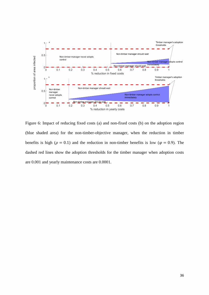
We take as an example a disease that has a high impact on timber benefits (𝜌 = 0.1) but little

effect on non-timber benefits (𝜑 = 0.9). In this case it is optimal for the timber manager to

adopt control immediately, providing that the proportion of infected area is within the region

[0.004, 0.8], while the non-timber manager should never adopt control. Figures 6 and 7 show

the adoption and cancellation regions respectively for the non-timber manager as the

proportional reduction in fixed costs, that is subsidy scheme 1 (top), and the reduction in

yearly costs, that is subsidy scheme 2 (bottom), increase. For comparison we also show the

adoption and cancellation thresholds for the timber manager. Note that we assume that both

subsidy schemes are only targeted at non-timber managers, so that is the timber managers’

costs remain fixed at the baseline values.

23

We find that both subsidy schemes switch the optimal strategy for the non-timber manager

from one where they should never adopt control to one where control should be adopted,

providing that the level of subsidy is large enough. Both types of subsidy thus succeed in

increasing the range of proportions of infected area for which the non-timber manager will

start to control, bringing the non-timber manager’s adoption thresholds closer to those of the

timber manager.

While the adoption thresholds behave in qualitatively the same way for both subsidy

schemes, this is not however the case for the cancellation thresholds. For subsidy scheme 1,

the upper cancellation threshold decreases, while the lower threshold increases as the

reduction in fixed costs increases (Figure 7a). Therefore, the overall effect is to increase the

size of the cancellation region as the reduction in costs increases. In particular, when fixed

costs are completely eliminated the adoption and cancellation thresholds are identical,

compare Figures 6a and 7a. This suggests that while there is a region over which it is optimal

for the non-timber manager to adopt control, they may cancel control almost immediately

upon adoption (if the proportion of area infected moves back into the cancellation region). On

the other-hand, for subsidy scheme 2, the cancellation thresholds behave in the same way as

the adoption thresholds, and so the size of the cancellation region decreases as yearly costs

are reduced (Figure 7b). Indeed if subsidy payments are large enough to remove all yearly

costs there is no longer a cancellation region. Therefore, once control has been adopted, the

non-timber manager will not cancel control.

This difference in the effects of differing subsidy types on the cancellation threshold suggests

that subsidising ongoing costs (rather than one-off upfront costs) may be more effective in

ensuring the continuation of disease control once it has been initiated. The intuition is that

both adoption and cancellation thresholds take account of future costs only. Once disease

control has started, a reduction in ongoing costs of control which are incurred each period

24

whilst control continues gives greater incentives to continue control than a reduction in the

costs of initiating control, which will only be incurred again if control is first discontinued

and then re-started.

4. Conclusions

There is a wide range of different management objectives amongst forests in the UK, as in

other countries. Understanding how this heterogeneity affects the disease control strategy

adopted by forest managers, and in particular when they will initiate control measures, is

therefore important for national decision-making institutions, such as DEFRA and the

Forestry Commission, whose aim is to minimise the spread of disease at the national, rather

than at the individual forest, level.

In this article we use a real options approach to investigate how forest management objectives

affect when (if ever) it is optimal for the manager of a forest to adopt control measures to

reduce damage due to disease, given that there is uncertainty in the future spread of infection.

Using the logistic SDE to describe the uncertainty in infection spread, unlike previous studies

(Saphores 2000; Saphores and Shogren 2005; Dixit and Pindyck 1994) which assume GBM,

we find that there exist two adoption thresholds, and similarly two cancellation thresholds.

The upper thresholds arise as a result of the bounded nature of the logistic SDE, which means

that when the level of infection is very high there is little to be gained from applying control

since most of the forest is infected, and so control should not be applied. Therefore, our

results show that control should only be initiated when the proportion of infected area lies

between these two thresholds, which we term the adoption region. The existence of two

adoption thresholds has important implications for decision makers as it suggests that, as well

as it being advantageous to wait when the area infected is low, it is also beneficial not to

25

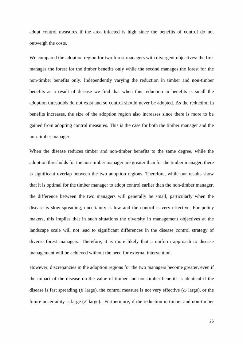
adopt control measures if the area infected is high since the benefits of control do not

outweigh the costs.

We compared the adoption region for two forest managers with divergent objectives: the first

manages the forest for the timber benefits only while the second manages the forest for the

non-timber benefits only. Independently varying the reduction in timber and non-timber

benefits as a result of disease we find that when this reduction in benefits is small the

adoption thresholds do not exist and so control should never be adopted. As the reduction in

benefits increases, the size of the adoption region also increases since there is more to be

gained from adopting control measures. This is the case for both the timber manager and the

non-timber manager.

When the disease reduces timber and non-timber benefits to the same degree, while the

adoption thresholds for the non-timber manager are greater than for the timber manager, there

is significant overlap between the two adoption regions. Therefore, while our results show

that it is optimal for the timber manager to adopt control earlier than the non-timber manager,

the difference between the two managers will generally be small, particularly when the

disease is slow-spreading, uncertainty is low and the control is very effective. For policy

makers, this implies that in such situations the diversity in management objectives at the

landscape scale will not lead to significant differences in the disease control strategy of

diverse forest managers. Therefore, it is more likely that a uniform approach to disease

management will be achieved without the need for external intervention.

However, discrepancies in the adoption regions for the two managers become greater, even if

the impact of the disease on the value of timber and non-timber benefits is identical if the

disease is fast spreading (𝛽 large), the control measure is not very effective (𝜔 large), or the

future uncertainty is large (𝐹 large). Furthermore, if the reduction in timber and non-timber

26

benefits due to the disease differ significantly then there can be substantial differences

between the timing of control measures for different types of manager. Indeed it can be

optimal for some managers to adopt control while for others it is never optimal to adopt

control. In these situations, particularly if the disease has differing impacts on timber and

non-timber benefits, for example dothistroma needle blight, the diversity of forest

management objectives creates tension in landscapes with multiple owner types, due to a

transferable externality (the disease).

Our results have important implications for policy makers since they show that the diversity

in management objectives alone does not lead to significantly different disease management

strategies between different manager types, but that it is a combination of the diversity in

management objectives and the way in which the disease affects these benefits that will

determine how uniform the adoption of control measures is at the landscape scale. Hence it is

important for decision makers to consider both these factors to ensure homogenous adoption

of control across the whole landscape.

When the impacts of a tree disease on the different benefits of a forest are divergent, we find

that subsidy schemes that reduce either the fixed cost or yearly maintenance cost can reduce

this discrepancy in the timing of initiation of disease control measures between different

types of forest manager. However, while under such a subsidy scheme the non-timber

manager will adopt control within a certain region, it is unlikely that such control measures

will be sustained in the long term. This is because the cancellation region becomes larger

with increasing subsidy payments (decreasing fixed costs) and when fixed costs are

eliminated then the cancellation and adoption thresholds coincide.

On the other-hand, a subsidy scheme that reduces yearly costs ensures that control measures

are more likely to be continued after initial adoption, since the size of the cancellation region

27

decreases as the subsidy payments increase (yearly costs decrease). This has implications for

policy makers on the performance of different types of subsidy schemes on aligning the

disease control strategies of different types of managers when the disease affects different

timber benefits in diverse ways. In particular, our results suggests that subsidy schemes

which reduce yearly maintenance costs may be more effective in ensuring continued

implementation of disease control measures over the longer term.

The main aim of this article is to investigate the effect of heterogeneity in management

objectives on the timing of control, rather than strategic interactions between forest managers

at the landscape scale. In particular, we have assumed that each forest manager makes

decisions independently of neighbouring forest managers. However, since the decision of a

manager to adopt control measures or not will impact on the spread of the disease to their

neighbours, for successful control a co-ordinated control response is needed. Epanchin-Niell

and Wilen (2015) consider the impact of local cooperative and coordinated control

agreements to manage invasions in a landscape with multiple independent identical

landowners. They find that the level of co-operation needed to mitigate damage caused by

disease depends on the cost of controls. In particular, their work shows that strategic

interactions between independent landowners can be important to ensure a successful control

response at the landscape scale. An interesting extension to the work presented here would be

to incorporate strategic interactions between two forest managers with differing objectives, so

as to investigate how the decision or whether or not to adopt control impacts the timing of

control adoption for a neighbouring forest manager with different objectives.

In this article we have considered a control measure that reduces that rate at which a tree

disease spreads, which could, for example, be the spraying of fungicides or pesticides that

reduce the susceptibility of trees, removal of weeds to increase the vigour of the trees and

reduce humidity or movement restrictions that reduce the chance of infected material being

28

bought in from elsewhere. However, other control measures involve the removal of infected

material, or treating currently infected trees, rather than altering the transmission rate

parameter. The model presented here could be extended to explore how the optimal timing of

control depends on the way in which a control measure alters disease spread. The model

could also be extended to consider the optimal timing of control over multiple timber rotation

periods, which would allow us to take into account that some non-timber benefits accumulate

over multiple rotations.

This article represents the first attempt to investigate how the interaction between future

uncertainty in disease spread and forest management objectives affect when (if ever) it is

optimal for an individual forest manager to adopt control measures to reduce damage due to

invasive pathogens or pests. We have shown that managers will adopt control at different

times depending on the management objectives of the forest, specifically what value is placed

on the various benefits from the forest, and the relative impact that disease has on these

different benefits. Furthermore, whilst subsidies always accelerate the adoption of disease

control measures (the adoption region widens), once control has been adopted, different

forms of subsidy can have opposite effects on the continuation of disease control (either

widening or narrowing the cancellation regions). Therefore, policy makers need to take into

account the range of different management objectives to ensure a uniform approach to

disease control at the landscape scale.

Acknowledgements

This work is funded jointly by a grant from BBSRC, Defra, ESRC, the Forestry Commission, NERC

and the Scottish Government, under the Tree Health and Plant Biosecurity Initiative.

29

Tables

Table 1: Parameter values used in numerical simulations.

Model Parameter Description Base case (Range)

𝛽 Initial infection transmission rate (i.e.

transmission rate when no control

deployed)

0.15

𝜔 Reduction in infection transmission rate

as a result of adopting control measures

0.1

𝐹 Magnitude of fluctuations in infection

transmission rate (uncertainty constant)

2.8

𝑏 Net value per hectare of annual non-

timber benefits

12⁄ 𝑟𝑒−𝑟𝑇/(1 − 𝑒−𝑟𝑇)

( 0 for timber manager,

𝑟𝑒−𝑟𝑇/(1 − 𝑒−𝑟𝑇) for non-

timber manager)

𝑝 Net return per hectare from timber sold 12⁄

(1 for timber manager, 0 for

non-timber manager)

𝜑 Factor by which non-timber benefits are

reduced as a result of infection

0.7 (in Figure 1),

0.4 (in Figure 5),

0.9 (in Figure 6,7),

(0, 1)

𝜌 Factor by which timber benefits are

reduced by as a result of infection

0.7 (in Figure 1),

0.4 (in Figure 5),

0.1 (in Figure 6,7),

(0, 1)

𝐾𝐴 Fixed cost of control measures 0.001 ([0, 0.001])

𝑚𝐴 Yearly maintenance cost of control

measures

0.0001 ([0, 0.0001])

𝛼 Proportion of initial sunk cost that is

recouped upon cancelling control

measures

0

𝑟 Risk-free interest rate 0.03

𝑇 Time period over which to consider the

value of the forest

80 years

30

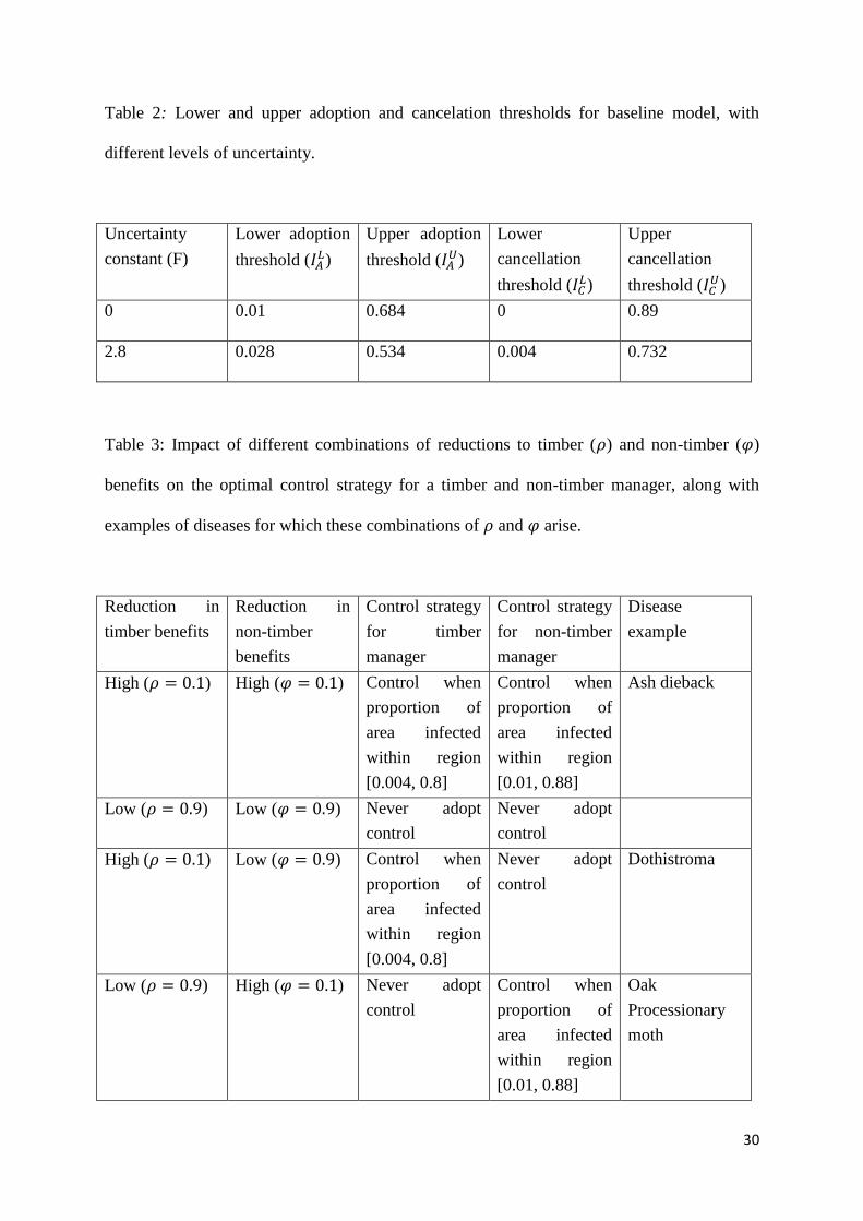
Table 2: Lower and upper adoption and cancelation thresholds for baseline model, with

different levels of uncertainty.

Uncertainty

constant (F)

Lower adoption

threshold (𝐼𝐴𝐿)

Upper adoption

threshold (𝐼𝐴𝑈)

Lower

cancellation

threshold (𝐼𝐶𝐿)

Upper

cancellation

threshold (𝐼𝐶𝑈)

0 0.01 0.684 0 0.89

2.8 0.028 0.534 0.004 0.732

Table 3: Impact of different combinations of reductions to timber (𝜌) and non-timber (𝜑)

benefits on the optimal control strategy for a timber and non-timber manager, along with

examples of diseases for which these combinations of 𝜌 and 𝜑 arise.

Reduction in

timber benefits

Reduction in

non-timber

benefits

Control strategy

for timber

manager

Control strategy

for non-timber

manager

Disease

example

High (𝜌 = 0.1) High (𝜑 = 0.1) Control when

proportion of

area infected

within region

[0.004, 0.8]

Control when

proportion of

area infected

within region

[0.01, 0.88]

Ash dieback

Low (𝜌 = 0.9) Low (𝜑 = 0.9) Never adopt

control

Never adopt

control

High (𝜌 = 0.1) Low (𝜑 = 0.9) Control when

proportion of

area infected

within region

[0.004, 0.8]

Never adopt

control

Dothistroma

Low (𝜌 = 0.9) High (𝜑 = 0.1) Never adopt

control

Control when

proportion of

area infected

within region

[0.01, 0.88]

Oak

Processionary

moth

31

Figures

Figure 1: Adoption (a and c) and cancellation regions (b and d) when there is no uncertainty

(c and d) and when uncertainty is included (a and b) in the decision problem (F=2.8).

Parameter values used for simulation are given in Table 1. Coloured regions show where

control should be adopted/cancelled immediately, while white regions show where the

manager should wait and see.

32

Figure 2: Stylised value of the forest if you adopt control and never cancel (green dot-dashed

line) and value of the forest if control is never adopted (red solid line). Note that these are the

value functions in the absence of any option values. The dotted green line indicates the value

of the forest if you adopt control and never cancel minus the cost of control.

33

Figure 3: Adoption regions for timber-objective manager (red) and non-timber-objective

manager (blue) when (a) the reduction in timber benefits equals the reduction in non-timber

benefits (1 − 𝜌 = 1 − 𝜑) and when (b) the reduction in timber benefits is not equal to the

reduction in non-timber benefits (1 − 𝜌 = 𝜑). Dashed lines show the switch points when

moving from a region where the adoption thresholds exist to one where control should never

be adopted.

34

Figure 4: Cancellation regions for timber-objective manager (red) and non-timber-objective

manager (blue) when (a) the reduction in timber benefits equals the reduction in non-timber

benefits (1 − 𝜌 = 1 − 𝜑) and when (b) the reduction in timber benefits is not equal to the

reduction in non-timber benefits (1 − 𝜌 = 𝜑). Dashed lines show the switch points when

moving from a region where the cancellation thresholds exists to one where control should

never be cancelled.

35

Figure 5: Upper and lower adoption thresholds for timber manager (blue dotted lines) and

non-timber manager (red solid lines) as a function of: (a) the transmission rate 𝛽, (b) the

reduction in transmission rate due to control 𝜔 and (c) the uncertainty parameter 𝐹. The

reduction to timber and non-timber is assumed to be fixed, 𝜌 = 𝜑 = 0.4.

36

Figure 6: Impact of reducing fixed costs (a) and non-fixed costs (b) on the adoption region

(blue shaded area) for the non-timber-objective manager, when the reduction in timber

benefits is high (𝜌 = 0.1) and the reduction in non-timber benefits is low (𝜑 = 0.9). The

dashed red lines show the adoption thresholds for the timber manager when adoption costs

are 0.001 and yearly maintenance costs are 0.0001.

37

Figure 7: Impact of reducing fixed costs (a) and non-fixed costs (b) on the cancellation region

(red shaded area) for the non-timber-objective manager, when the reduction in timber

benefits is high (𝜌 = 0.1) and the reduction in non-timber benefits is low (𝜑 = 0.9). The

dashed green lines show the cancellation thresholds for the timber manager when adoption

costs are 0.001 and yearly maintenance costs are 0.0001.

38

References

Dangerfield, CE, AE Whalley, N Hanley, and CA Gilligan. 2016. “What a Difference a

Stochastic Process Makes: Epidemiologicalbased Real Options Models of Optimal

Treatment of Diseaseitle.” In Prep. http://www.st-andrews.ac.uk/media/dept-of-

geography-and-sustainable-development/pdf-s/DP 2016-03 Dangerfield et al.pdf.

Dixit, Avinash, and Robert Pindyck. 1994. Investment Under Uncertainty. Princeton

University Press.

Epanchin-Niell, R. S., and J. E. Wilen. 2015. “Individual and Cooperative Management of

Invasive Species in Human-Mediated Landscapes.” American Journal of Agricultural

Economics 97 (1): 180–98. doi:10.1093/ajae/aau058.

Fitter, Alistair. 1980. Trees. Collins Gem.

Freer-Smith, Peter H., and Joan F. Webber. 2015. “Tree Pests and Diseases: The Threat to

Biodiversity and the Delivery of Ecosystem Services.” Biodiversity and Conservation.

Springer Netherlands. doi:10.1007/s10531-015-1019-0.

Hanley, Nick, and Morag MacPherson. 2016. “Economics of Invasive Pests and Diseases: A

Guide for Policy Makers and Managers.” University of St Andrews Discussion Papers in

Environmental Economics.

Insley, Margaret. 2002. “A Real Options Approach to the Valuation of a Forestry Investment

1.” Journal of Environmental Economics and Management 44: 471–92.

Keeling, Matt J, and Pejman Rohani. 2008. Modeling Infectious Diseases In Humans and

Animals. Princeton University Press.

Marten, Alex L., and Christopher C. Moore. 2011. “An Options Based Bioeconomic Model

for Biological and Chemical Control of Invasive Species.” Ecological Economics 70

39

(11). Elsevier B.V.: 2050–61. doi:10.1016/j.ecolecon.2011.05.022.

Ndeffo Mbah, Martial L, Graeme a Forster, Justus H Wesseler, and Christopher a Gilligan.

2010. “Economically Optimal Timing for Crop Disease Control under Uncertainty: An

Options Approach.” Journal of the Royal Society, Interface / the Royal Society 7 (51):

1421–28. doi:10.1098/rsif.2010.0056.

Saphores, J. 2000. “Pest Population : A Real Options Approach.” American Journal of

Agricultural Economics 82: 541–55.

Saphores, Jean-daniel. “Barriers and Optimal Investment Rules. 1,” no. 949.

Saphores, Jean-Daniel M., and Jason F. Shogren. 2005. “Managing Exotic Pests under

Uncertainty: Optimal Control Actions and Bioeconomic Investigations.” Ecological

Economics 52 (3): 327–39. doi:10.1016/j.ecolecon.2004.04.012.

Sims, Charles, and David Finnoff. 2012. “The Role of Spatial Scale in the Timing of

Uncertain Environmental Policy.” Journal of Economic Dynamics and Control 36 (3).

Elsevier: 369–82. doi:10.1016/j.jedc.2011.09.001.

———. 2013. “When Is a ‘wait and See’ Approach to Invasive Species Justified?” Resource

and Energy Economics 35 (3). Elsevier B.V.: 235–55.

doi:10.1016/j.reseneeco.2013.02.001.

Sims, Charles, David Finnoff, and Jason F Shogren. 2016. “Bioeconomics of Invasive

Species : Using Real Options Theory to Integrate Ecology , Economics , and Risk

Management.” Food Security. doi:10.1007/s12571-015-0530-1.

Sturrock, R. N., S. J. Frankel, A. V. Brown, P. E. Hennon, J. T. Kliejunas, K. J. Lewis, J. J.

Worrall, and A. J. Woods. 2011. “Climate Change and Forest Diseases.” Plant

Pathology 60 (1): 133–49. doi:10.1111/j.1365-3059.2010.02406.x.

40

Urquhart, Julie, and Paul Courtney. 2011. “Seeing the Owner behind the Trees: A Typology

of Small-Scale Private Woodland Owners in England.” Forest Policy and Economics 13

(7). Elsevier B.V.: 535–44. doi:10.1016/j.forpol.2011.05.010.

Wilmott, P, S Howison, and J Dewynne. 1995. The Mathematics of Financial Derivatives.

Cambridge University Press.

41

Appendix

We solve the free boundary problem given by equations (10) and (11) along with the

boundary conditions given by equations (6) to (9), (12) and (13) in MATLAB using the Euler

method (Wilmott, Howison, and Dewynne 1995). To ensure numerical convergence, the time

step used for numerical simulation, 𝑑𝑡, must satisfy the following condition,

𝑑𝑡 <1

2(𝜎 × 𝑑𝐼)2 ,

where 𝑑𝐼 is the mesh size for the infected area variable (𝐼) that is used in simulation (we take

𝑑𝐼 = 0.002 in all simulations). Since this is a free-boundary problem, in order to solve the

problem numerically, an upper boundary condition must be stipulated in the case where 𝐼 = 1

as well as a lower boundary condition in the case where 𝐼 = 0. Therefore, we assume that

∂2𝑊𝐴∂I2⁄ =

∂2𝑊𝐶∂I2⁄ = 0 at 𝐼 = 1, 0 which is used to obtain the finite difference scheme

at the upper boundary (Insley 2002).