DRAFT – October 2005 – DRAFT

The Effects of Name and Sector Concentrations on the Distribution of Losses for Portfolios

of Large Wholesale Credit Exposures*

Erik Heitfield Federal Reserve Board erik.heitfield@frb.gov

Steve Burton Federal Deposit Insurance Corporation

sburton@fdic.gov

Souphala Chomsisengphet Office of the Comptroller of the Currency souphala.chomsisengphet@occ.treas.gov

Abstract: This paper examines the influence of systematic and idiosyncratic risk on credit losses for portfolios of large wholesale bank loans. Information on banks’ largest credit exposures from US bank regulators’ Syndicated National Credits (SNC) examination program and a hierarchical factor model calibrated from KMV data are used to simulate the distribution of portfolio credit losses for 30 real-world loan portfolios. We find that for very large SNC portfolios idiosyncratic risk is of limited importance, but it can meaningfully increase Value-at-Risk (VaR) for smaller portfolios. The average contribution of systematic risk to Value-at-Risk is similar in groups of relatively large and relatively small SNC portfolios. Simple indexes of name and sector concentration are positively correlated with portfolio VaR even after controlling for differences in average credit quality and portfolio size. We use Monte Carlo simulations to estimate the marginal contribution to portfolio VaR of credit exposures to individual sectors and find that exposures to different economic sectors have dramatically different influences on VaR. These differences result not only from variation in the average credit quality of obligors across sectors, but also from features of the dependence structure of credit losses. The relative importance of expected loss, systematic risk, and idiosyncratic risk varies considerably from sector-to-sector and is sensitive to the distribution of exposures within a given portfolio.

* The views expressed here are solely those of the authors. They do not reflect the opinions of the Federal Reserve Board of Governors, the Federal Deposit Insurance Corporation, or the Office of the Comptroller of the Currency.

1. Introduction

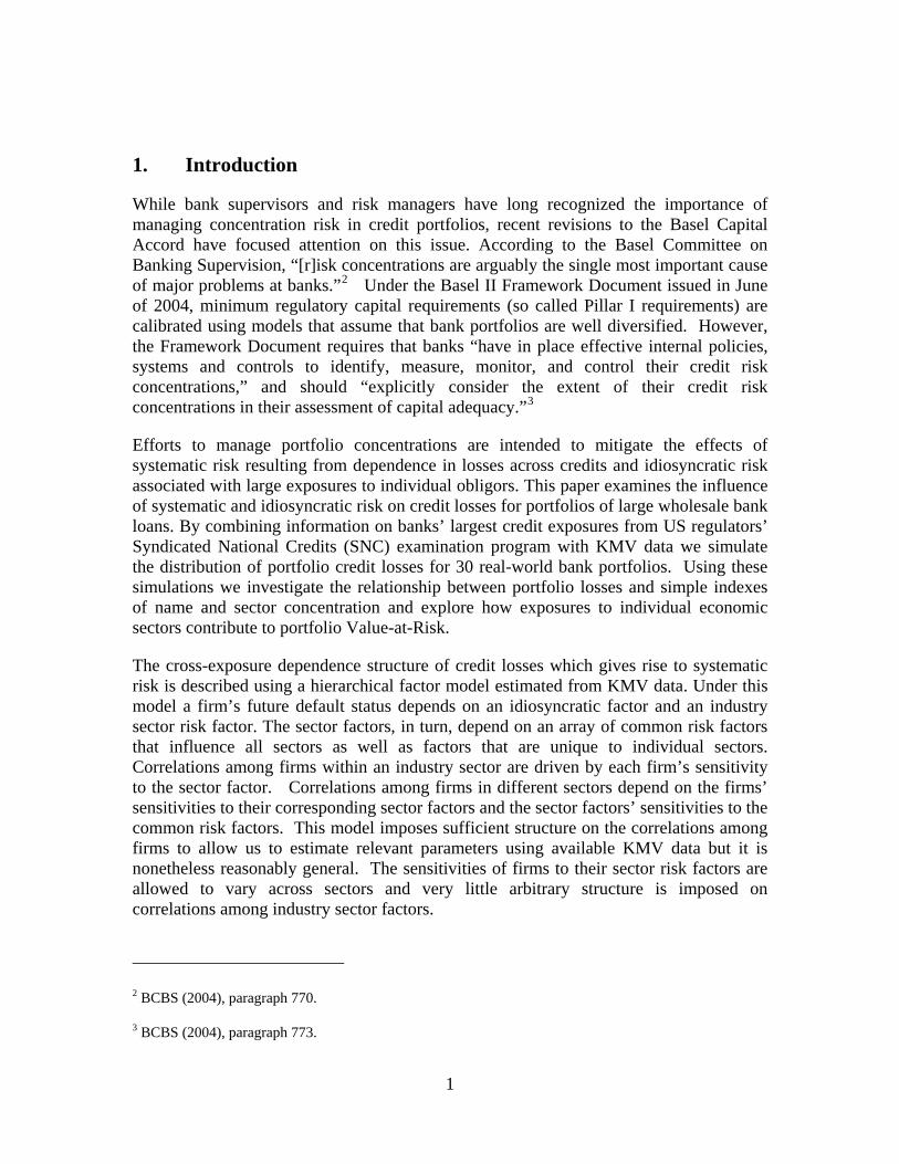
While bank supervisors and risk managers have long recognized the importance of managing concentration risk in credit portfolios, recent revisions to the Basel Capital Accord have focused attention on this issue. According to the Basel Committee on Banking Supervision, “[r]isk concentrations are arguably the single most important cause of major problems at banks.”2 Under the Basel II Framework Document issued in June of 2004, minimum regulatory capital requirements (so called Pillar I requirements) are calibrated using models that assume that bank portfolios are well diversified. However, the Framework Document requires that banks “have in place effective internal policies, systems and controls to identify, measure, monitor, and control their credit risk concentrations,” and should “explicitly consider the extent of their credit risk concentrations in their assessment of capital adequacy.”3

Efforts to manage portfolio concentrations are intended to mitigate the effects of systematic risk resulting from dependence in losses across credits and idiosyncratic risk associated with large exposures to individual obligors. This paper examines the influence of systematic and idiosyncratic risk on credit losses for portfolios of large wholesale bank loans. By combining information on banks’ largest credit exposures from US regulators’ Syndicated National Credits (SNC) examination program with KMV data we simulate the distribution of portfolio credit losses for 30 real-world bank portfolios. Using these simulations we investigate the relationship between portfolio losses and simple indexes of name and sector concentration and explore how exposures to individual economic sectors contribute to portfolio Value-at-Risk.

The cross-exposure dependence structure of credit losses which gives rise to systematic risk is described using a hierarchical factor model estimated from KMV data. Under this model a firm’s future default status depends on an idiosyncratic factor and an industry sector risk factor. The sector factors, in turn, depend on an array of common risk factors that influence all sectors as well as factors that are unique to individual sectors. Correlations among firms within an industry sector are driven by each firm’s sensitivity to the sector factor. Correlations among firms in different sectors depend on the firms’ sensitivities to their corresponding sector factors and the sector factors’ sensitivities to the common risk factors. This model imposes sufficient structure on the correlations among firms to allow us to estimate relevant parameters using available KMV data but it is nonetheless reasonably general. The sensitivities of firms to their sector risk factors are allowed to vary across sectors and very little arbitrary structure is imposed on correlations among industry sector factors.

2 BCBS (2004), paragraph 770.

3 BCBS (2004), paragraph 773.

1

We use the hierarchical factor model to investigate the effects of systematic and idiosyncratic risk on the distribution of losses for banks’ syndicated loan portfolios. Among the different types of credit exposures held by banks, syndicated loans are especially useful for studying the implications of sector and name concentrations.4 These credit exposures, as represented by SNC examination data, account for an estimated one-third or more of large U.S. agent banks’ total corporate loan exposures, and consist primarily of exposures to large domestic and multinational companies. As such, the performance of syndicated loans often provides a window into broader corporate credit trends and credit conditions.5 For instance, the credit deterioration experienced by various large U.S. banking organizations during the recessionary period of 2000 to 2002 corresponded to a significant rise in problem syndicated loans as identified through the SNC program. Because they represent loan exposures of the largest firms within any given sector, syndicated loan exposures also serve as a meaningful barometer of industry conditions and trends.

By simulating the distribution of losses for syndicated credit portfolios, we are able to decompose portfolio Value-at-Risk into expected, systematic, and idiosyncratic risk components. We find that both idiosyncratic and systematic risk can have significant effects on the distribution of losses for banks’ large wholesale credit portfolios. For very large SNC portfolios idiosyncratic risk is of limited importance, but it meaningfully increases Value-at-Risk for smaller portfolios. Banks with relatively small SNC portfolios may therefore need to more actively manage concentrations to individual obligors than banks with larger portfolios, or they may need to hold additional capital to offset the effects of idiosyncratic risk. The average contribution of systematic risk to Value-at-Risk is similar in groups of relatively large and relatively small SNC portfolios. Although larger portfolios tend to be better diversified across sectors than smaller ones, portfolio size alone does not appear to substantially mitigate the effects of systematic risk.

Simple indexes of name and sector concentration are positively correlated with portfolio Value-at-Risk, even after controlling for differences in average obligor credit quality and portfolio size. However, though correlated with VaR, these indexes cannot fully explain observed variation in VaR among the 30 SNC portfolios we study. Concentration indexes based only on portfolio exposure weights can provide useful metrics for assessing the extent to which bank exposures are diversified across sectors or names, but because they are not sensitive to cross-sector differences in exposure characteristics they are of limited utility for managing exposures to individual sectors or obligors.

4 Syndicated loans are large corporate loan exposures held by a group (or syndicate) of lenders.

5 See http://www.federalreserve.gov/boarddocs/press/bcreg/2002/20021008/default.htm.

2

In order to effectively manage name and sector concentrations banks need to compare the relative impact of exposures to different sectors on portfolio loss distributions. We use Monte Carlo simulations to estimate the marginal contribution of credit exposures to individual sectors to portfolio Value-at-Risk and find that different economic sectors have dramatically different influences on VaR. These differences result not only from variation in the average credit quality of obligors in different sectors, but also from features of the dependence structure of credit losses across sectors. The relative importance of expected loss, systematic risk, and idiosyncratic risk varies from sector-to-sector and is sensitive to the distribution of exposures within a particular SNC portfolio. Thus, efforts to manage name concentration can be expected to have a greater impact on VaR in some sectors and portfolios than others. The benefits of reducing aggregate exposures to particular sectors will similarly vary across sectors and will depend on the weighting of sector exposures within a given portfolio.

The paper is organized as follows. Section 2 describes the SNC examination data used in this analysis. Section 3 introduces several simple concentration measures that can be calculated with a minimum of information on the sector weighting and number of exposures within a portfolio. Sections 4 and 5 discuss calibration of the hierarchical factor model and show how it can be used to simulate the distribution of realized credit losses for a portfolio of loans. In Sections 6 and 7 we examine the relationship between observable portfolio characteristics and the distributions of simulated portfolio losses. Section 6 focuses on three bank portfolios in detail while Section 7 investigates patterns in the full sample of 30 bank portfolios. Section 8 shows how Monte Carlo simulations can be used to estimate the marginal contribution of exposures in different sectors to portfolio VaR and applies this approach to selected SNC portfolios. Section 9 summarizes conclusions and shows how they relate to recent empirical and theoretical research on the management of credit risk in bank loan portfolios.

2. Portfolios of Syndicated National Credits

The SNC examinations program provides U.S. banking supervisors with an important source of information about corporate credit market trends and conditions. This program was developed in 1977 for the primary purpose of ensuring the consistency and accuracy of supervisory risk ratings for commonly-shared syndicated loan exposures held by regulated banking organizations. The program is supported by a database that is updated annually with SNC exposure information. Reporting requirements are triggered when a syndicated loan commitment exceeds $20 million and when that exposure is held by three or more regulated entities.6 Based on the most recently available 2005 SNC data, the SNC database captures nearly $1.7 trillion in commercial credit exposures to roughly 4,700 borrowers. These exposures represent an estimated one-third of the total commercial loan exposures (on and off-balance sheet) of U.S. regulated banking organizations. With an average credit exposure of $350 million per borrower, the 6 That is, regulated by one of the three U.S. federal bank regulators: the Federal Reserve System, the Office of the Comptroller of the Currency, or the Federal Deposit Insurance Corporation.

3

database predominantly reflects credit exposures of large domestic and multinational corporations.

We analyze the SNC portfolios for the 30 largest SNC lenders as measured by the total dollar value of SNC commitments in 2005. Taken together, these banks hold roughly $760 billion in SNC commitments, which represents about 46 percent of the total value of commitments included in the SNC examination database. Among these banks are the largest US commercial banks, as well as smaller regional, monoline, and processing banks.

For each bank SNC exposures are grouped into 50 broadly-defined industry sectors. These industry sectors are comprised of companies in economically related financial and non-financial businesses as determined by each firm’s primary industry classification code using either North American Industry Classification System (NAICS) or Standard Industrial Classification (SIC) codes. The composition of each of these 50 broad sectors, based on SIC codes, is detailed in Table 1.

The SNC database includes detailed information on each SNC exposure, but for this analysis we use sector-level data. For each of the banks in our sample we have compiled data on the total dollar value of SNC commitments in each industry sector and the number of SNC exposures to each sector. Importantly, our data do not included information on the size distribution of exposures within a sector or the identities of the obligors associated with individual exposures. For this reason, we assume that all of a bank’s commitments to a particular sector are the same size. Thus, for example, if the total loan commitment by a bank to the Aerospace and Defense sector is fifty-million dollars and the bank has extended 10 loans to this sector, we assume that the commitment amount for each facility is five-million dollars. Throughout this paper, we will use ws to denote the portfolio weight on sector s as measured by the sector’s share of total commitments. We will use ns and n to denote the number of exposures in sector s and the number of exposures in the portfolio respectively.

Table 2 reports information on the distribution and the number of SNC exposures by industry sector for the aggregate portfolio containing all syndicated national credits including those held by banks not represented in our sample. As we shall see presently, this “All SNC” portfolio provides a useful benchmark for assessing the degree of concentration of individual bank portfolios. To provide a sense of the relative credit quality of exposures in each sector, Table 2 also reports sector-wide average KMV EDFs.7

7 Some institutions in our sample have a small number of SNC exposures to real-estate investment trusts (REITs) which are not included in this analysis. As discussed in Section 3, our model of credit losses is calibrated using imputed asset values and EDFs from KMV. While KMV publishes EDFs for some REITs, it recommends that these parameters be treated with particular caution. An obligor’s EDF and imputed asset value is sensitive to its liability structure which, in the case of a REIT, can change rapidly. Because data on REIT liability structures are updated relatively infrequently, a REIT’s EDF may not reflect its current liability structure, and conversely, its EDF may change dramatically as new liability information becomes available.

4

Because of the confidential nature of SNC examination data, we cannot report detailed information on the sector distribution of syndicated credit exposures for individual institutions. To preserve the anonymity of bank-level information and to aid in summarizing the available SNC data, we have divided the 30-bank sample into banks with small, medium, and large SNC portfolios. Small portfolios are defined as those with total commitments of less than $10 billion; medium portfolios are those with total commitments between $10 and $20 billion; and large portfolios are those with total commitments of greater than $20 billion. The rows labeled “Portfolio Characteristics” in Table 3 report summary information on the portfolios in each of the three size categories as well as the All SNC portfolio.

3. Simple indexes of name and sector concentration

The credit risk for a portfolio of exposures at some future horizon can be decomposed into three components: expected loss (EL), systematic risk, and idiosyncratic risk. Expected loss refers to that component of future losses that can be forecast from currently-available information on the characteristics of portfolio exposures. Because it can be predicted, EL can be managed relatively easily by appropriately pricing newly-originated loans and by setting aside reserves for seasoned loans that have declined in credit quality. Systematic risk is that component of portfolio losses attributable to dependence in losses across individual credit exposures. Typically, systematic risk is modeled as arising from common shocks that affect many obligors at once. This risk component can be managed but it cannot be eliminated. Banks can lessen the influence of systematic risk by shifting lending toward exposures whose losses tend to be less highly correlated with one another. For example, if losses on loans to obligors within an economic sector tend to be more highly correlated than those of loans to obligors in different sectors, then spreading exposures across sectors may reduce the volatility of portfolio losses. Idiosyncratic risk refers to that component of future losses that can potentially be diversified away. Typically, idiosyncratic risk is seen as arising from independent shocks to individual obligors. In principle, by distributing exposures in a portfolio across a large number of obligors, idiosyncratic risk can be largely eliminated.

Equity capital serves as a buffer to cover unexpected portfolio losses arising from systematic and idiosyncratic risk. Efforts by banks to limit exposures to particular economic sectors or to individual obligors are intended to reduce unexpected losses, thereby lessening the need for costly capital. Indexes designed to measure “name concentration” and “sector concentration” are often used to summarize the distribution of exposures within a portfolio across obligors or sectors. In this section we describe typical examples of such indexes and use them to compare SNC portfolios. In Sections 6 and 7 we will examine how these indexes are related expected loss and systematic and idiosyncratic risk in these portfolios.

Broadly speaking, name concentration refers to any granularity in exposures to individual obligors within a portfolio. Gordy (2003) suggests a standard for measuring name concentration. He defines an infinitely-fine-grained portfolio as one in which no exposure to a single obligor is large enough relative to the total portfolio to meaningfully

5

affect the realized portfolio loss rate. In practice, of course, no portfolio can achieve this level of diversification across names, but the infinitely-fine-grained portfolio serves as a useful benchmark for measuring name concentration. The name-concentration Herfindahl index

2s

N ss

whn

≡∑

provides a simple measure of the deviation of an actual portfolio from the infinitely-fine-grained portfolio benchmark. This index reflects information about both the number and the relative sizes of individual obligor exposures in a portfolio. A portfolio consisting of only one exposure would have a Herfindahl index equal to one and a portfolio consisting of an infinite number of very small exposures – Gordy’s infinitely-fine-grained portfolio – would have a Herfindahl index of zero.

An alternative to measuring name concentration relative to a theoretical fully diversified portfolio is to measure such concentration relative to a well diversified market portfolio. In this analysis we will use the All SNC portfolio as a benchmark for assessing name concentration. Let ws

* and ns* denote the sector exposure weight and the number of

obligors in sector s for the All SNC portfolio. We define the name-concentration entropy index as

( ) ( )( )( )( )

* *

* *

ln ln

ln mins s s s ss

Ns s s

w w n w ne

w n

−≡ −∑

.

This index is equal to zero if all obligor exposures in the portfolio receive the same weight as those in the All SNC portfolio and it approaches one in the limiting case where the portfolio weight on the single obligor with the smallest weight in the All SNC portfolio grows to dominate all others. If the sector exposure weights and the relative number of exposures in each sector are held constant, then eN is decreasing in the number of exposures in the portfolio.8

Sector concentration is a bit harder to define than name concentration. Since the number of industry sectors is finite and fixed, it is not meaningful to consider a benchmark diversified portfolio in which exposure to any given sector is so small that no sector has a significant effect on portfolio losses. It also would not be particularly meaningful to assume that a diversified portfolio is one in which each sector receives equal weight because some sectors clearly play a much larger role in the economy than others. For

8 Note that both hN and eN are derived under the assumption that all exposures within a sector are the same size so that the portfolio weight on obligor i in sector s is ws/ns. These measures are only approximations to those indexes that would be calculated from actual obligor exposure weights. hN will understate the “true” name concentration Herfindahl index.

6

these reasons, it is particularly desirable to assess sector concentration relative to a real-world benchmark portfolio. The sector-concentration entropy index

( ) ( )( )( )( )

*

*

ln ln

ln mins s ss

Ss s

w w we

w

−≡ −∑

provides a measure of the difference between a portfolio’s sector exposure weights and those of the All SNC portfolio. This entropy index has the following appealing properties: (i) when all weight in a bank portfolio is concentrated in that sector with the smallest weight in the All SNC portfolio eS = 1, (ii) when the bank sector weights are equal to those of the All SNC portfolio eS = 0, and (iii) in all other cases eS lies between zero and one.

The sector-concentration Herfindahl index is defined as

2S ss

h w≡∑ .

While hS is commonly used to summarize sector concentration, it has some unappealing features. It is very sensitive to sector definitions. For example, if two large sectors are aggregated together, hS may increase substantially. Moreover, in contrast to the entropy measure, the Herfindahl index is insensitive to differences in the overall size of different sectors. This measure attains a minimum when a portfolio is equally weighted across all sectors, even though some sectors are presumably much larger than others.

The rows labeled “Concentration Indexes” in Table 3 report SNC portfolio group averages, minimums, and maximums of the four measures of portfolio concentration discussed above. As expected, smaller portfolios appear by our measures to be more concentrated than larger portfolios. However, notice that for all four concentration measures there are substantial overlaps in the range of index values across groups. Thus, there is not a strict decreasing relationship between portfolio size and either name or sector concentration.

Table 4 reports Kendall correlation coefficients among the four concentration indexes calculated for the 30 SNC portfolios in our sample.9 The entropy and Herfindahl indexes of name concentration are very highly correlated, suggesting that both these measures convey similar information. The entropy and Herfindahl indexes of sector concentration are somewhat less highly correlated, so there may be some advantage in using one of these indexes over the other. The name- and sector- concentration indexes are positively correlated with one another because, in general, larger portfolios tend to be less concentrated across both names and sectors.

9 Unlike the more common Pearson correlation coefficient, Kendall’s tau is invariant to monotone transformations of the variables of interest. Hence it provides a better indication of whether two indexes convey similar information.

7

None of the concentration indexes discussed here are directly linked to standard portfolio risk metrics such as Value-at-Risk. While it is intuitive to think that a portfolio that is more evenly distributed across names or sectors may be less subject to the effects of idiosyncratic and systematic risk, the relationship between portfolio exposure weights and the distribution of portfolio credit losses is quite complex and – except under very stylized assumptions – it cannot be accurately described using simple portfolio-wide concentration indexes.10 To fully understand the roles of expected, systematic, and idiosyncratic risk in credit portfolios a model of the dependence of credit losses across exposures is needed.

4. Modeling dependence in exposure losses

To model dependence in credit losses across exposures we use a framework based on Merton (1974) similar to that underlying industry-standard credit risk models such as those developed by KMV (Crosbie and Bohn, 2005) and the Risk Metrics Group (Gupton, Finger, and Bhatia, 1997). Under this framework the default status of firm i at a one-year-ahead assessment horizon depends on the realization of a continuous index of the firm’s credit quality denoted Yi. This variable is commonly interpreted as a measure of the firm’s return on assets over the assessment horizon. If the realized value of Yi lies below a critical default threshold γi then firm i defaults and exposures to that firm accrue a credit loss; if the realized value of Yi exceeds the default threshold no loss arises from exposures to the firm. The probability of default of firm i is simply the probability that Yi lies below γi. For simplicity we assume that the loss-given-default (LGD) per dollar exposure is exogenous and is the same for all firms. Given this framework, the loss rate per dollar exposure to firm i is

(1) 0 if

if >⎧

= ⎨ ≤⎩i i

ii i

YL

YLGDγγ

We assume that Yi can be expressed as the sum of two risk factors: an idiosyncratic risk factor that is unique to firm i and a sector risk factor that affects all firms in firm i’s industry sector. If firm i is part of sector s then

(2) 21i s s i sY Z Eλ λ= + −

where Zs is the sector risk factor, Ei is the idiosyncratic risk factor, and λs is a sector-specific parameter that lies between zero and one. Zs and Ei are standard normal random variables that are independent of one-another so that, by construction, the marginal distribution of Yi is also standard normal. λs, the sector factor loading, describes the

10 One can conclude that as the name-concentration Herfindahl index approaches zero the contribution of idiosyncratic risk to portfolio losses approaches zero as well. However, there is no direct relationship between values of this index that are different from zero and the magnitude of the contribution from idiosyncratic risk at the portfolio level.

8

sensitivity of firms in sector s to the sector risk factor Zs. Notice that a higher value for λs implies that firm i is more sensitive to the industry factor and less sensitive to the idiosyncratic factor.

We next assume that each sector risk factor can be expressed as a linear combination of K common factors and one sector-specific factor. The sector risk factor for sector s is defined as

(3) ' 1s s s sZ U= + −X ω ω 'ωs

1

where X is a K-dimensional standard normal random vector of common risk factors, Us is a standard normal random variable that is independent of X, and ωs is a K-dimensional parameter vector that is normalized so that ' ≤s sω ω . ωs, the common factor loadings, describes the sensitivity of the sector risk factor Zs to the vector X of common factors. Because all sector risk factors depend on some or all of the common factors, the sector risk factors will be correlated with one-another. The magnitude and direction of such correlations depends on each the common factor loadings for each sector.

Correlations in loss rates across firms are driven by correlations in the firms’ credit quality indexes. Consider firm i in sector s and firm j in sector t. Equations (2) and (3) imply that

(4) ( ) ( )

2 if Cor ,

if '⎧ =⎪= ⎨ ≠⎪⎩

si j

s t s t

s tY Y

s tλ

λ λ ω ω.

Observe that when λs is high, credit losses for two firms in sector s will be highly correlated with one another. The correlation in loss rates among exposures to two firms in different industry sectors depends on each firm’s sensitivity to its sector risk factor and the two sector risk factors’ sensitivities to the common risk factors. All else equal, losses for exposures to two firms in the same sector are more likely to occur together than losses for two firms in different sectors.11 Under this simple model estimates of the sector factor loading λs and estimates of each sector’s common factor loadings ωs are all that are needed to describe dependencies in loss rates across exposures.

To estimate the factor loadings, we use monthly KMV data on the asset values for 4,516 large corporate firms with average historical asset values exceeding $500 million between 1993 and 2004. For each firm it rates, KMV imputes an asset value from data on the firm’s leverage and its equity price and volatility.12 We use these imputed assets 11 A single-risk-factor model consistent with the assumptions used to derive minimum regulatory capital requirements under Basel II arises as a special case of the hierarchical model in which for every sector s, ωs’ ωs = 1. In this special case all sector factors are perfectly correlated, and the correlation between Yi and Yj is simply the product of the sector factor loadings for firms i and j.

12 The details of this procedure are proprietary to KMV Corporation, but the basic methodology is described by Crosbie and Bohn (2005). Treating equity as a call option on the assets of a firm, KMV

9

values to construct annual rates of return on assets for each firm which can stand in as proxies for the credit quality indexes, Yi. Equation (4) implies that the sector factor loading λs is equal to the square-root of the pair-wise correlation between Yi and Yj for any two firms i and j in sector s. Using this fact, we estimate each sector’s sector factor loading as the square-root of the average empirical correlation between all pairs of obligors in the sector.

Table 5 reports estimated sector factor loadings. As can be seen from these results, the correlation among the asset returns of the firms in a sector varies considerably across sectors. Returns for firms in the Oil Refining and Delivery sector, for example, appear to move together rather closely while those of firms in the Commercial Banking sector appear to be much less correlated with one-another. In interpreting these figures it is important to keep in mind that although the asset returns for firms in a sector may not be highly correlated, the aggregate returns for the sector as a whole may nonetheless be closely linked with those of other sectors. Within a sector the fortunes of individual firms may differ for a variety of largely idiosyncratic reasons including management quality, market power, and even simple luck. In aggregate the idiosyncrasies associated with individual firms should average out so that sector-wide returns may tend to more directly reflect fundamental economic drivers of profitability. To investigate the relationship among returns in different sectors it is therefore useful to examine correlations among sector-wide mean returns captured in our model by industry sector risk factors.

Normalized annual average rates of return for each industry sector provide proxies for the sector factors and the empirical correlation among these proxy sector factors provides an estimate of the correlation matrix of sector factors. Deriving estimated common factor loadings from an empirical correlation matrix is a standard factor analysis problem. Let Z be the vector of sector factors (Zs) for each of S sectors and let Ω be a K-by-S matrix whose columns are the K-dimensional common factor loadings (ωs). Equation (3) implies that

(5) [ ] ( )Cor ' diag 'S= + −Z Ω Ω I Ω Ω .

Given the empirical proxy sector factor correlation matrix, a standard iterative principle components method is used to derive parameters for Ω that minimize discrepancies between the left- and right-hand-sides of equation (5). The estimates presented here assume six common factors (K = 6). Several other specifications of K were considered. The majority of the correlation among sectors can be explained by only one common factor. Adding common factors beyond the first six does little to improve the fit of the model.

Estimated common factor loadings for each sector are reported in Table 5. Shaded cells identify large loadings of particular interest. If two sectors have loadings on a given

inverts an options pricing formula to impute a firm’s asset price and volatility from observable data on firm leverage and the value and volatility of equity.

10

factor that are large in magnitude and share the same sign then aggregate returns for these sectors tend to be more highly correlated with one another. Interpreting loadings from a multifactor model is a notoriously ambiguous exercise that invariably involves a degree of judgment. Nonetheless an examination of the estimated common factor loadings provides insights into the relationships among sector returns. Loadings on the first common factor are all the same sign and are relatively large in magnitude. This factor would seem to capture the influence of a general macroeconomic cycle on all sectors. Loadings on the second factor suggest high correlations in returns among high-tech sectors. Large loadings on the third and fourth factors point to high correlations among returns in fossil energy and other resource extraction sectors. Loadings on the fifth factor suggest that the fortunes of firms in Healthcare and Medical Equipment sectors tend to move together.

5. Simulating portfolio losses

To examine the roles of expected loss, systematic risk, and idiosyncratic risk in SNC portfolios we use Monte Carlo simulation to estimate portfolio loss distributions. We assume that all credit losses occur at the end of a one-year horizon and arise only from obligor defaults. This default-mode approach abstracts from exposure revaluation effects that arise in a mark-to-market setting when exposures have maturities longer than one year. As mentioned earlier, we assume that the loss-given-default for all exposures is non-stochastic.13 Finally, we assume that the amount of an exposure at default is 100% of the current exposure commitment amount. Taken together, these assumptions imply that the only source of uncertainty surrounding a portfolio’s one-year-ahead loss rate is the default status of obligors.

For practical reasons we all loans within a sector as if the were interchangeable, ex ante. The dataset used in this analysis provides information on the total dollar value of loan commitments by in each sector and the number of obligors in each sector. It does not include the credit amounts committed to individual obligors, so we assume that all loans within a given sector receive equal weight in the portfolio. Because we do not know the counterparty associated with individual exposures, we assume that each obligor has a PD equal to the average KMV EDF for all SNC exposures in that obligor’s sector.14

Given these stylized assumptions, the loss per dollar exposure to sector s is

13 For all exposures we assume an LGD of 45 percent. This is consistent with the regulatory treatment for unsecured wholesale exposures under Basel II’s foundation internal-ratings-based approach. If LGD were stochastic but independent across exposures, it would contribute to idiosyncratic risk. If it were stochastic and was not independent across exposures, it would contribute to both idiosyncratic and systematic risk.

14 If PD is the average KMV EDF for sector s then for each obligor i in sector s we set γ = Φ (PD ). It is easy to verify that given this calibration equation (1) implies that the one-year-ahead unconditional default probability for each obligor in sector s is equal to PD .

s i-1

s

s

11

(6) ss

s

DL LGDn

= ⋅

where Ds in an integer-valued random variable that describes the number of defaults in the sector. Ds depends on idiosyncratic and sector risk factors. Since we assume that all obligors in a sector share the same default probability, the expected loss per dollar exposure to sector s is simply

(7) [ ]E s sL PD LGD= .

Conditional on the sector risk factor Zs, Ds is a binomial random variable composed of ns independent Bernoulli trials. Equations (1) and (2) imply that the expected loss rate for sector s given the sector risk factor Zs is

(8) [ ] ( )E |s s s sL Z p Z LG= D

where

( ) ( )1

21s s s

s s

s

PD Zp Z

λ

λ

−⎛ ⎞Φ −⎜ ⎟= Φ⎜ ⎟−⎝ ⎠

The Law of Large Numbers implies that as ns grows large for a given realization of Zs equation (6) converges in probability to equation (8).15

The loss rate per dollar exposure in a portfolio of sector exposures is

(9) s ssL w L=∑ .

Equation (9) can be decomposed in a way which allows us to parse out the incremental effects of expected loss, systematic risk, and idiosyncratic risk on portfolio losses. Observe that

(9’) [ ] [ ] [ ]( ) [ ]( )A B C

E E | E Es s s s s s s s s ss s s

L w L w L Z L w L L Z= + − + −∑ ∑ ∑ |

Term A in this expression is the portfolio expected loss rate. It is non-stochastic and can be readily calculated using equation (7). Term B is that component of the portfolio loss rate that can be attributed to common shocks within and across sectors. Term C is that component of the portfolio loss that can be attributed to lack of diversification across names within sectors. As the number of exposures in all sectors grows large, Term C approaches zero for any realization of the sector risk factors.

15 See Vasicek (1991) for a derivation of (8).

12

The distribution of L for a given bank portfolio is estimated using Monte Carlo simulation. We first draw a realization of each sector risk factor Zs using equation (3) and the estimated common factor loadings. For each sector we then simulate the loss rate per dollar exposure conditional on the realized sector risk factor by drawing a value of Ds from a binomial distribution with ns trials and success probability ps(Zs). Finally, we use equations (6) and (9) to calculate a realized portfolio loss rate which embeds the effects of both systematic and idiosyncratic risk. For each simulated draw of L, equation (9’) can be used to decompose the loss rate into expected, systematic, and idiosyncratic components. By simply dropping term C from the simulated loss calculations we are able to derive the portfolio loss distribution consistent with the assumption of perfect diversification across names.

6. The role of systematic risk and idiosyncratic risk in selected portfolios

In this section we compare simulated loss distributions for three bank portfolios chosen from the portfolio-size groups described in Section 2. We have deliberately selected three portfolios with similar expected losses to allow us to focus on the effects of systematic and idiosyncratic risk on portfolio loss distributions.

Table 6 reports concentration indexes for the three portfolios. As expected, smaller portfolios have greater name concentrations as measured by the entropy and Herfindahl concentration indexes. Note, however, that the entropy and Herfindahl indexes give conflicting information about the relative importance of sector concentration in the Small Bank portfolio. The Herfindahl index suggests that this portfolio is less concentrated among sectors than the Medium Bank or Large Bank portfolio, while the entropy index suggests that it is more concentrated.

The Lorenz curves in Figure 1 provide a more detailed look at the distribution of portfolio exposures across sectors. The difference between a portfolio’s Lorenz curve and the 45-degree line indicates a difference between the portfolio sector weights and the All SNC portfolio weights. In the figure cumulative sector weights are calculated based on a sorting of sectors from highest to lowest average EDF, so a Lorenz curve above the 45-degree line indicates a portfolio that is weighted toward sectors with higher average default probabilities relative to the All SNC portfolio. As can be seen from this figure, the Large Bank portfolio is slightly more weighted toward particularly low- and particularly high-EDF sectors than the All SNC portfolio. The differences between the Medium Bank and Small Bank portfolios and the All SNC portfolio are more significant. Both portfolios are substantially less weighted toward sectors with particularly high EDFs than the All SNC portfolio and contain a larger share of exposures in sectors with mid-range EDFs..

For each portfolio 400,000 Monte Carlo trials were used to simulate the distribution of portfolio losses at a one-year horizon. Table 7 reports characteristics of the simulated loss distributions with and without incorporating the effects idiosyncratic risk. Density plots of the simulated loss distributions are shown in Figure 2. Incorporating

13

idiosyncratic risk in the loss simulations has no effect on expected loss, but shifts mass to the tail of the loss distribution.

Table 8 decomposes the Value-at-Risk for each portfolio into expected, systematic, and idiosyncratic risk components based on equation (9’). VaR is defined as the 99.9th percentile of the loss distribution. Unexpected loss (UL) is defined as the difference between VaR and EL and reflects the combined effects of systematic and idiosyncratic risk.16 In all four portfolios the majority of Value-at-Risk is attributable to unexpected loss, and most of UL arises from systematic risk.

While the Large Bank portfolio has lower EL than the All SNC portfolio, it has slightly higher UL. The effects of systematic risk are greater in the Medium Bank portfolio than in either the All SNC or the Large Bank portfolios. The UL per dollar exposure attributed to systematic risk for the Medium Bank portfolio is about seven percent larger than that of the All SNC portfolio. The systematic risk component of UL for the Small Bank portfolio is only slightly larger than that of the Medium Bank portfolio.

For the All SNC and the Large Bank portfolios, idiosyncratic risk plays very little role. It increases UL for the All SNC portfolio by less than one percent and it increases UL for the Large Bank portfolio by about 1.5 percent. Name concentration has a somewhat larger effect in the Medium Bank portfolio; it increases UL by about 3.3 percent. The effect of name concentration is very significant in the Small Bank portfolio. Idiosyncratic risk increases UL for the Small Bank portfolio by about 10 percent.

These comparisons suggest that idiosyncratic risk can meaningfully increase Value-at-Risk and UL for smaller SNC portfolios that are less well diversified across names. Systematic risk is the most important contributor to VaR and UL for all portfolios, but larger portfolios that are better diversified across sectors do appear to be somewhat less affected by systematic risk. In the next section we examine the relationship between portfolio size, indexes of name and sector concentration, and unexpected loss for a broader set of SNC portfolios.

7. The relationship between SNC portfolio characteristics and Value-at-Risk

The comparison of simulated loss distributions for three banks’ SNC portfolios in the previous section suggests that differences in portfolio size and name and sector concentration measures are closely related to the distribution of realized credit losses. This section examines the relationship between portfolio characteristics and the distribution of portfolio losses for our full sample of 30 SNC portfolios. The rows labeled “Components of Value-at-Risk” in Table 3 report information on the distribution of estimated expected and unexpected loss rates for the large, medium, and small SNC

16 This definition of unexpected loss is consistent with that used to calculate minimum regulatory capital requirements under Basel II’s internal-ratings-based approaches.

14

portfolio segments of our sample. As can be seen from the statistics on portfolio expected loss there is no clear relationship between portfolio size and EL. On average, the medium- and small-portfolio groups have lower EL than either the large portfolio group or the All SNC portfolio. The range of expected losses among the small portfolio group is considerably larger than that among the other two groups. Because smaller portfolios are less diversified across sectors, exposures to particular high- or low-credit-quality sectors tend to have larger influences on the EL of these portfolios, leading to greater dispersion of ELs among members of the small-portfolio group.

Table 3 also suggests no clear relationship between portfolio size and unexpected losses arising from systematic and idiosyncratic risk. As with EL, the dispersion in UL across portfolios is greatest for the small-portfolio group. Portfolios in the medium size group have the lowest UL on average, whether or not simulated UL estimates reflect the effects of name concentration. Not surprisingly, idiosyncratic risk affects UL more for smaller portfolios than for larger ones. On average, accounting for the effects of name concentrations increases UL by 3.3 percent, 5.5 percent, and 12.9 percent for the large-, medium-, and small-portfolio groups respectively.

Figure 3 shows the components of portfolio VaR attributed to expected loss, systematic risk, and idiosyncratic risk for each of the SNC portfolios in our sample. As can be seen from this figure, in every case systematic risk is by far the largest contributor to portfolio VaR.17 While expected loss is correlated with VaR, there is not a one-to-one relationship between expected and unexpected losses. The portfolio with the lowest EL in our sample has the lowest VaR and the portfolio with the highest EL has the highest VaR, but for other portfolios there is no clear relationship between EL and either the systematic- or the idiosyncratic-risk components of UL.

Table 9 reports parameter estimates for regressions of portfolio characteristics on simulations of UL (including both systematic and idiosyncratic risk) for the full sample of 30 SNC portfolios.18 Specification (a) confirms that portfolio size (as measured by total exposure) and EL are closely related to portfolio UL. However, a comparison of specifications (a), (b), and (d) suggests that entropy indexes of name and sector concentration are much more informative about portfolio UL than is portfolio size. Including the entropy indexes and omitting portfolio size (specification (b)) provides a much better fit than including size but omitting the entropy indexes (specification (a)).. Adding size to a model that includes the entropy indexes (specification (d)) does little to improve the fit of the model. Comparing specifications that use entropy indexes

17 The relative importance of systematic risk and expected loss as contributors to portfolio VaR depends on the loss percentile used to define VaR. The systematic risk contribution is increasing in the loss percentile while the expected loss contribution is fixed. Our conclusions reflect a 99.9th percentile VaR measure which is consistent with the solvency standard used in Basel II and may be somewhat less conservative than that used internally by banks.

18 A two-step generalized-least-squares procedure was used to correct for heteroscadasticity associated with portfolio size and EL.

15

(specifications (b) and (d)) with those that use Herfindahl indexes (specifications (c) and (e)) suggests that the two entropy indexes are more informative about portfolio UL than are the two Herfindahl indexes. The sector concentration Herfindahl index appears to be of little value for assessing UL. In both specifications that involve the Herfindahl indexes, the sector concentration Herfindahl index is not statistically significant, and in specification (c) it has the wrong sign.

While we find a positive relationship between simple portfolio-wide concentration indexes and unexpected loss, it is important to note that a significant share of observed variation in UL across SNC portfolios is not explained by a combination of expected loss, portfolio size, and concentration indexes. Under specification (e), which provides the best fit among the specifications considered, these factors explain just over three-quarters of the cross-portfolio variation in UL. As discussed in Section 3, portfolio-wide concentration indexes can provide useful summary information on the overall distribution of exposures within a portfolio, but they are too simplistic to fully capture the effects of systematic and idiosyncratic risk on portfolio losses. By their nature, concentration indexes treat exposures to all sectors or obligors in a symmetric fashion. As we shall see in the next section, exposures to different sectors can have very different effects on the distribution of portfolio losses.

8. Managing exposures to individual sectors

The risk associated with a particular exposure can be managed by evaluating that exposure’s marginal contribution to portfolio-wide risk measures such as Value-at-Risk, expected loss, or unexpected loss. For example, it is common to allocate economic capital to a credit exposure commensurate with its marginal contribution to portfolio UL. Similarly, loan-loss provisions may be allocated based on an exposure’s expected loss. Not all exposures contribute equally to portfolio loss measures. Obviously, lower quality credits (in our model, exposures to higher-PD obligors) tend to contribute more to both expected and unexpected portfolio credit losses. What is perhaps less well appreciated is that differences in exposure portfolio weightings and the dependence structure of losses across exposures can have significant influences on an exposure’s marginal contribution to UL, VaR, and other portfolio risk measures. In this section we use Monte Carlo simulations based on the hierarchical factor model developed in Section 4 to examine differences across sectors’ marginal contributions to portfolio VaR. These marginal effects are decomposed into UL and EL components, and the marginal UL contributions are further decomposed into components arising from systematic and idiosyncratic risk.

Let lα be the αth percentile of the portfolio loss rate L. For a specified value of α (99.9 percent in this analysis) lα is the portfolio Value-at-Risk. L depends on the portfolio sector weights so lα depends on these weights as well. To show how one can measure the effect on lα of a small changes in sector weights, we need to introduce some additional notation. Let Es be the vector of obligor-specific idiosyncratic risk factors for exposures in sector s, and let F = Z1…ZS,E1…ES be the vector of all sector risk factors and idiosyncratic factors. Given a realization f of F, the portfolio loss rate is fully determined. The default rate for sector s is

16

(10) ( ) 21, 1 1s

s s s s s i s si Cs

d z z en

λ λ γ∈

= + −∑e <

where Cs is the set of exposures in sector s. The portfolio loss rate is

(11) . ( ) ( ),s s s ssw d z LGD=∑f e

L is discrete, whereas F is continuous. Thus, a given realization of L is consistent with a continuum of realizations of F. The set of realizations of F consistent with the αth percentile of L is

(12) ( ) 0 | lα αℑ = =f f .

Using a result from Gourieroux, Laurent, and Scaillet (2000, Lemma 1) it can be shown that

(13) ( ) 0E , |∂ ⎡ ⎤= ∈ℑ⎣ ⎦∂E Fs s s

s

l d Z LGDwα

α .

Equation (13) gives a unique expression for the marginal effect on portfolio VaR of an increase in investment in sector s. In principle, this expression can be used to calculate the marginal contribution of an exposure to sector s. In practice, however, evaluating the conditional expectation in (14) may not be tractable. When a portfolio contains more than a trivially small number of name exposures, it is impractical to write down a set of constrains on F consistent with membership in 0

αℑ . In this case, Monte Carlo simulation can be used to approximate (14).

The set

(14) ( ) | lεα α εℑ = − <f f

describes realizations of F that produce portfolio loss rates that lie in a neighborhood of the αth percentile of L. Observe that

(15) ( ) ( ) 0

0lim E , | E , |s s s s s sd Z d Zε

α αε→⎡ ⎤ ⎡ ⎤∈ℑ = ∈ℑ⎣ ⎦ ⎣ ⎦E F E F .

Equations (13) and (15) suggest the approximation

(16) ( )E , |∂ ⎡ ⎤≈ ∈ℑ⎣ ⎦∂E Fs s s

s

l d Z LGDw

εαα .

The approximation can be made as precise as desired by choosing a sufficiently small value for ε. For a given value of ε the conditional expectation in (16) can be estimated as a by-product of the Monte Carlo simulation procedure described in Section 5. Recall that

17

to simulate the distribution of L we first generated pseudo-random draws from the marginal distribution of F. Given a sufficiently large number of such draws, a conditional expectation of any function of F can be approximated using Monte Carlo integration and acceptance sampling. The conditional expectation in equation (16) is approximated by computing the average value of ( ),s s sd z e evaluated over all those

pseudo-random draws of F that are members of εαℑ .

When Monte Carlo integration is used to estimate the conditional expectations in equation (16), choosing ε involves a tradeoff. A smaller value of ε improves the accuracy of the approximation described in the equation, but it means that fewer pseudo-random draws are available for estimating the conditional expectation. For this analysis, we set ε = 0.0002. Thus, to estimate marginal contributions for the 99.90th percentile of L we average over pseudo-random draws of the risk factors that are consistent with realized loss rates between the 99.88th and 99.92th percentiles of L. Our Monte Carlo simulation consists of 400,000 draws from the marginal distribution of F which gives us 160 draws with which to evaluate the conditional expectation.19

Using equations (7) and (8), we can rewrite equation (16) as

(16’) ( )

( ) ( )

A

B

C

E |

E , |

≈

⎡ ⎤+ − ∈ℑ⎣ ⎦

⎡ ⎤+ − ∈ℑ⎣ ⎦

F

E F

ss

s s s

s s s s s

l PD LGDw

p Z PD LGD

d Z p Z LGD

α

εα

εα

δδ

Equation (16’) provides a decomposition of the marginal contribution for sector s. Term A is the component that can be attributed to the expected loss of exposures in the sector; term B is that component arising from dependence in defaults across exposures in the sector (systematic risk); and term C is that component arising from name concentration within the sector (idiosyncratic risk).

Figure 4 shows the marginal contribution per dollar exposure to VaR by sector for the All SNC portfolio For selected sectors, Table 10 and Figure 5 compare the marginal contributions to VaR for the All SNC portfolio and the three bank portfolios described in Section 6. For each sector the marginal contributions are separated into components attributable to expected loss, systematic risk, and idiosyncratic risk.

19 With very minor modifications, the method described here can be used to estimate marginal contribution to other measures of portfolio risk such as expected tail loss (ETL). In fact, for a given number of Monte Carlo simulation and a given threshold loss percentile, marginal contributions to ETL can probably be estimated with greater accuracy because more pseudo-random draws are available for approximating the conditional expectation (i.e. the acceptance region is larger).

18

The most striking feature of these results is the dramatic differences in marginal VaR contribution across sectors. For example, in the All SNC portfolio a one-dollar increase in exposure to the Oil and Gas Exploration sector adds less than a penny to VaR while an additional dollar of exposure to the Telecommunications sector adds about 15 cents. Some portion of cross-sector differences in VaR contribution can be attributed to differences in the average credit quality of obligors, but this is not the whole story. Again comparing contributions for the All SNC portfolio, we see that while both the Oil and Gas Exploration sector and the Electric, Gas, and Sanitary sector have similar expected losses (both roughly 0.23 percent) the marginal VaR contribution for the Electric, Gas, and Sanitary sector is nearly double that of the Oil and Gas Exploration sector (1.31 percent versus 0.69 percent). All else equal, sectors whose losses are more highly correlated with aggregate portfolio losses contribute more to portfolio VaR.

Though less dramatic than the cross-sector differences, there are also important differences in the level and character of marginal contributions associated with exposures to the same sectors in different SNC portfolios. The marginal contribution of a one-dollar increase in the Telecommunication sector, for example is 16.5 cents in the Large Bank portfolio and 11.5 cents in the Medium Bank portfolio – a difference of about one-third. Such differences can be attributed to differences in portfolios’ sector exposure weights and to differences in diversification across names within sectors. Not surprisingly, in the Small Bank portfolio a greater share of the marginal contribution to VaR for most sectors can be attributed to idiosyncratic risk.

These results suggest that the most effective strategies for managing the effects of systematic and idiosyncratic risk on portfolio losses will differ across sectors and should be tailored to the particular features of a bank’s loan portfolio. In some sectors defaults are rare but they tend to be highly correlated with one-another and with overall portfolio losses. In such cases it may be most effective to manage aggregate exposure to the sector as a whole rather than working toward greater diversification among names within the sector. In other sectors where defaults among obligors are less highly correlated, reducing name concentration may be more effective. In general, for relatively large SNC portfolios name concentrations within individual sectors appears to contribute little to portfolio VaR. Systematic risk, on the other hand, plays an important role in all sectors and portfolios.

9. Implications for credit-risk management

Systematic risk is an important contributor to portfolio Value-at-Risk for both large and small SNC portfolios. Indeed for all of the 30 SNC portfolios studied, systematic risk accounts for a significantly greater share of portfolio VaR than either expected loss or idiosyncratic risk. Larger SNC portfolios appear to be somewhat better diversified across economic sectors than smaller ones, and a simple entropy index of sector concentration is positively correlated with portfolio VaR. The marginal contribution of systematic risk to portfolio VaR varies greatly across sectors, however, so that even banks with large and relatively well-diversified SNC portfolios can benefit from economic capital systems and sector concentration limits that accurately reflect sector differences.

19

Though considerably less important than systematic risk, idiosyncratic risk can also have a meaningful influence on the distribution of portfolio credit losses and hence on bank solvency and capital adequacy. For banks with smaller SNC portfolios that are not particularly well diversified across names, name concentrations can appreciably increase unexpected losses. For example, we estimate that for a group of nine relatively small SNC portfolios (each with less than $10 billion in total exposure) idiosyncratic risk increases UL over a one-year horizon by more than ten percent on average. The effect for individual banks can be significantly larger. Banks with smaller SNC portfolios may therefore need to more actively manage name concentrations and/or they may need to hold additional economic capital against this source of risk.

In order to effectively manage systematic and idiosyncratic risk, banks need to understand how each exposure in a credit portfolio influences the distribution of future portfolio losses. Analytic work in this area has made extensive use of a single-systematic-risk-factor framework under which losses for individual exposures are assumed to be conditionally independent given a scalar systematic factor. Gordy (2003) demonstrates that given this assumption one can derive a simple closed-form expression for the systematic-risk component of an exposure’s marginal contribution to portfolio Value-at-Risk. Analytic results surveyed by Martin and Wilde (2002) can be used to asses the influence of idiosyncratic risk on portfolio losses under the single-systematic-risk-factor assumption.

Despite its theoretical appeal, empirical research by Akhavein, Kocagil, and Neugebauer (2005), Wendin and McNeil (2005), and Carling, Ronnegard, and Roszbach (2004) suggests that a single-systematic-risk-factor framework is not adequate to fully describe portfolio credit losses. All else equal, the credit losses associated with exposures to obligors in the same industry sectors appear to be more highly correlated with one another than those associated with exposures to obligors in different sectors. Hence, both sector-specific and common risk factors are needed to describe the dependence structure of credit losses within a portfolio. The analysis of imputed asset-value data from KMV presented in Section 3 confirms this finding.20

As shown in Section 8, Monte Carlo simulations can be used to estimate an exposure’s marginal contribution to portfolio VaR and to determine the shares of that contribution attributable to expected loss, systematic risk, and idiosyncratic risk. In principle this approach can be applied under a very wide range of parametric models of credit loss dependence. It does not require that one impose a single systematic risk factor assumption and is therefore compatible with models in which both common risk factors and sector-specific factors influence credit losses. Unfortunately, this flexibility comes at a price. The number of Monte Carlo simulations needed to obtain accurate estimates of sector-specific marginal contributions to VaR is exceptionally large, particularly when VaR is pegged to a high percentile of the portfolio loss distribution. Less 20 This is not a new result. KMV’s own analyses of its data finds support for a model with industry- and country-specific risk factors and such a model is embedded in its Porfolio ManagerTM product (Zeng Zhang, 2001).

20

computationally burdensome analytic approaches to assessing the influence of name or sector exposures on portfolio loss distributions in the presence of sector-specific common risk factors would clearly be of practical value. Recent theoretical research by Hanson, Pesaran, and Schuermann (2005) on the effects of obligor heterogeneity on portfolio losses and by Emmer and Tasche (2003) on semi-analytic approaches to measuring VaR contributions may prove useful in this regard.

21

Works Cited

Akhavein, Jalai D. Ahmet E Kocagil, and Matthias Neugebauer. 2005. “A comparative empirical study of asset correlation.” Fitch Ratings, Quantitative Financial Research Special Report. (Fitch Ratings Ltd.: New York).

Basel Committee on Banking Supervision (BCBS). 2004. International Convergence in Capital Standards, A Revised Framework. (BIS: Basel).

Carling, Kenneth, Lars Ronnegard, and Kasper Roszbach. 2004. “Is firm interdependence within industries important for portfolio credit risk?” Sveriges Riksbank Working Paper Series, no. 168.

Crosbie, Peter and Jeff Bohn. 2005. “Modeling default risk.” White Paper. (Moodys/KMV Corp.: New York).

Emmer S. and D. Tasche. 2003. “Calculating credit risk capital charges with the one factor model.” Unpublished working paper.

Gordy, Michael. 2003. “A risk factor model foundation for ratings-based bank capital rules.” Journal of Financial Intermediation, v. 12, pp. 199-232.

Gupton, Greg, Christopher C. Finger, and Mickey Bhatia. 1997. CreditMetrics – Technical Document. (J. P. Morgan and Co.: New York).

Gourieroux, C., J. P. Laurent, and O. Scailet. “Sensitivity analysis of Value at Risk.” Journal of Empirical Finance, v. 7. 2000. pages 225-245.

Hanson, Samual, M. Hashem Pesaran, and Til Schuermann. 2005. “Scope for credit risk diversification.” Institute of Economic Policy Research Working Paper.

Merton, Robert. 1974. “On the pricing of corporate debt: the risk structure of interest rates.” Journal of Finance, v. 29, pp. 449-470.

Vasicek, Oldrich A. 1991. “Limiting loan loss probability distributions.” White Paper. (KMV LLC: San Francisco).

Wendin, Jonathan and Alexander McNeil. 2005. “Dependent credit migrations.” National Centre for Competence in Research, Financial Valuation and Risk Management Working Paper, no. 182.

Zeng, Bin and Jing Zhang. 2001. “An empirical assessment of asset correlation models.” White Paper. (KMV LLC: San Francisco).

22

Table 1: Industry sector definitions

Industry Sector Sector Composition by Standard Industrial Code (SIC) ClassificationAerospace & Defense 3480-3489, 3720-3728, 3760-3764, 3811-3812Agriculture 100-299, 700-799, 900-999, 5083, 5153-5159, 5191, 5193, 5992Air Transportation 4500-4581Apparel, Footwear, & Textiles 2200-2399, 3100-3199, 3960, 5131-5139, 5611-5699, 5948-5949Automotive 3000-3011, 3700-3716, 5012-5015, 5511-5531, 5561, 5599Broadcast Media 4830-4841, 4891, 4899Business Services 7300-7371, 7373-7399Chemicals 2800-2899, 5169, 5912Commercial Banks 6020-6023, 6712Computer Equipment 3570-3579, 5045, 5734, 7372Construction 1500-1799, 2451-2452, 5032-5039, 5074, 5082, 5198, 5271Consumer Credit & Credit Card Financing 6141Electric, Gas, & Sanitary 4900-4991Electronics & Electrical 3600-3673, 3675-3699, 5063-5065, 5075-5078, 5731Entertainment & Leisure 5091-5092, 5735-5736, 5941, 5945, 7800-7999, 8400-8499Fabricated Metals 3400-3479, 3490-3499Food, Beverages, & Tobacco 2000-2141, 5141-5149, 5181-5182, 5194, 5411-5499, 5921, 5962, 5993General Retail 5200-5799, 5900-5999, 5311, 5331, 5399, 5932, 5943, 5947, 5961, 5963, 5999Glass & Stone 3200-3299Healthcare 5122, 5995, 8000-8999Insurance 6300-6499Legal & Other Services 8100-8399, 8500-8999Lodging 7000-7099Machinery & Equipment 3500-3569, 3580-3599, 3820-3832, 5043-5044, 5046, 5084-5087, 5261, 5722, 5946Medical Equipment 3821, 3841-3851, 5047-5049Mining 1000-1099, 1200-1241, 1400-1499, 5052, 5094, 5944Miscellaneous Manufacturing 3860-3959, 3961-3999, 5093, 5095-5099, 5199Mortgage Credit 6160-6163Nonbank Investment 6700-6711, 6713-6797, 6799Nondefense Trans. & Parts 3717-3719, 3729-3759, 3765-3799, 5088, 5551, 5571Oil Refining & Delivery 2900-2999, 4600-4699, 5171-5172, 5541, 5983-5989Oil & Gas Exploration 1300-1389Other Depository & Trust 6000-6019, 6024-6099, 6111Other Nondepository Credit 6131, 6150-6159, 6172Other Trans. Services 4000-4199, 4300-4399, 4700-4799Paper & Forestry 800-899, 2411-2448, 2490-2499, 2600-2679, 5112-5113Personal Services 7200-7299Primary Metals 3300-3399, 5051Printing & Publishing 2700-2796, 5111, 5192, 5942, 5994REITS 6798Real Estate Operators 6500-6553Repair Services & Rental 7500-7699Restaurants 5800-5813Rubber & Plastics 3012-3099, 5162Securities Broker/Dealers 6200-6299Semiconductors 3674Telecommunications 4810-4822, 4892Trucking & Warehousing 4200-4299Water Transportation 4400-4499Wood, Furniture, & Fixtures 2400-2410, 2449, 2453-2489, 2500-2599, 5021-5031, 5072, 5211-5251, 5712-5719

23

Table 2: Distribution of all Syndicated National Credit exposures among sectors

Sector Exposure Weight

Number of Names

Average EDF

Aerospace & Defense 2.32% 62 1.09% Agriculture 0.67% 72 1.24% Air Transportation 0.27% 18 3.14% Apparel, Footwear, & Textiles 1.26% 126 0.88% Automotive 3.81% 222 1.69% Broadcast Media 3.19% 121 2.95% Business Services 1.69% 165 4.37% Chemicals 3.13% 212 1.26% Commercial Banks 0.63% 48 0.28% Computer Equipment 0.72% 51 4.72% Construction 3.24% 402 2.03% Consumer Credit & Credit Card Financing 3.67% 51 3.57% Electric, Gas, & Sanitary 7.95% 585 0.50% Electronics & Electrical 1.34% 133 2.88% Entertainment & Leisure 2.49% 245 3.15% Fabricated Metals 1.23% 142 1.75% Food, Beverages, & Tobacco 4.70% 378 0.57% General Retail 2.28% 129 1.52% Glass & Stone 0.48% 33 1.36% Healthcare 2.86% 280 2.48% Insurance 3.85% 168 0.47% Legal & Other Services 1.18% 181 3.00% Lodging 1.65% 123 2.63% Machinery & Equipment 2.70% 266 1.49% Medical Equipment 0.72% 64 1.27% Mining 0.44% 46 1.34% Miscellaneous Manufacturing 1.36% 128 1.70% Mortgage Credit 1.42% 65 9.27% Nonbank Investment 4.95% 219 0.93% Nondefense Trans. & Parts 0.16% 15 0.91% Oil Refining & Delivery 1.76% 142 1.08% Oil & Gas Exploration 4.07% 206 0.51% Other Depository & Trust 0.33% 22 0.16% Other Nondepository Credit 4.09% 166 1.68% Other Trans. Services 1.65% 81 0.55% Paper & Forestry 1.73% 109 0.53% Personal Services 0.50% 37 2.25% Primary Metals 0.79% 78 2.85% Printing & Publishing 2.07% 166 0.46% Real Estate Operators 2.69% 343 1.50% Repair Services & Rental 0.97% 85 5.28% Restaurants 0.65% 81 2.47% Rubber & Plastics 1.37% 138 3.78% Securities Broker/Dealers 1.92% 98 0.99% Semiconductors 0.18% 14 2.11% Telecommunications 5.17% 227 8.14% Trucking & Warehousing 0.38% 56 0.67% Water Transportation 0.38% 38 0.57% Wood, Furniture, & Fixtures 0.95% 136 0.38%

24

Table 3: Characteristics of small, medium, and large portfolio groups

Large Portfolios

Medium Portfolios

Small Portfolios

All SNC Portfolioa > $20

Billion $10 - $20

Billion < $10 Billion

Number of institutions represented 3,528 10 9 11

Portfolio size in $ billions (averages for portfolio groups) 1,630.1 58.1 13.6 4.8 Portfolio

Characteristics Number of exposures in portfolio

(averages for portfolio groups) 7,088 2,166 804 312

Minimum 0.022 0.175 0.247 Average 0.147 0.241 0.353 Name-concentration

entropy index Maximum

0b

0.246 0.317 0.417 Minimum 0.000 0.001 0.001 Average 0.001 0.002 0.005 Name-concentration

Herfindahl index Maximum

0.000 0.003 0.004 0.008

Minimum 0.003 0.032 0.040 Average 0.021 0.040 0.093 Sector-concentration

entropy index Maximum

0b

0.038 0.056 0.175 Minimum 0.030 0.032 0.035 Average 0.037 0.045 0.074

Concentration Indexes

Sector-concentration Herfindahl index

Maximum 0.033

0.045 0.072 0.213 Minimum 0.71% 0.74% 0.54% Average 0.91% 0.82% 0.83% Expected Loss

Maximum 0.90%

1.04% 0.95% 1.18% Minimum 3.61% 3.43% 2.54% Average 3.90% 3.72% 3.98% Unexpected loss from

systematic risk Maximum

3.81% 4.31% 4.21% 5.33%

Minimum 3.71% 3.57% 3.44% Average 4.02% 3.93% 4.49%

Components of Value-at-Risk

Unexpected loss from systematic and

idiosyncratic risk Maximum 3.84%

4.40% 4.33% 5.71% Notes a: Entries in the “All SNC Portfolio” column reflect information for the aggregate portfolio of all SNC credits. Entries for all other columns reflect statistics for portfolio size groups. b: Index is zero by construction.

25

Table 4: Kendall correlations among indexes of name and sector concentration

Name-concentration entropy index

Name-concentration Herfindahl index

Sector-concentration entropy index

Name-concentration Herfindahl index 0.876

Sector-concentration entropy index 0.724 0.710

Sector-concentration Herfindahl index 0.517 0.586 0.582

26

Table 5: Estimated loadings for the hierarchical factor model Common Factor Loadings (in order of significance) Sector Sector

Loading 1 2 3 4 5 6 Aerospace & Defense 0.427 0.883 0.235 -0.094 -0.102 0.168 0.007 Agriculture 0.468 0.714 0.293 -0.313 -0.233 0.088 0.156 Air Transportation 0.558 0.772 0.016 -0.058 0.405 0.168 -0.295Apparel, Footwear, & Textiles 0.396 0.850 0.320 0.163 0.081 -0.094 -0.033Automotive 0.462 0.810 0.292 -0.079 -0.172 -0.075 -0.345Broadcast Media 0.447 0.547 -0.730 -0.181 0.143 -0.217 -0.174Business Services 0.438 0.573 -0.711 -0.256 -0.189 -0.069 -0.209Chemicals 0.354 0.691 -0.531 0.222 0.254 0.229 0.128 Commercial Banks 0.288 0.548 0.194 -0.527 0.404 -0.389 -0.081Computer Equipment 0.521 0.496 -0.849 -0.007 -0.105 0.059 -0.059Construction 0.415 0.816 0.206 0.184 0.329 0.068 -0.297Consumer Credit & Credit Card Financing 0.237 0.717 -0.199 0.275 0.114 0.348 0.018 Electric, Gas, & Sanitary 0.482 0.483 0.130 0.012 0.730 0.218 -0.037Electronics & Electrical 0.510 0.532 -0.813 0.152 -0.091 -0.014 0.041 Entertainment & Leisure 0.374 0.868 -0.001 0.069 -0.154 -0.069 -0.242Fabricated Metals 0.528 0.861 0.167 -0.031 0.024 -0.027 0.351 Food, Beverages, & Tobacco 0.399 0.804 0.476 -0.186 0.010 0.059 -0.006General Retail 0.340 0.793 -0.075 -0.146 -0.269 -0.231 -0.351Glass & Stone 0.447 0.721 0.434 -0.137 -0.138 -0.143 -0.132Healthcare 0.443 0.691 0.115 -0.051 -0.030 0.372 0.327 Insurance 0.381 0.775 0.440 -0.090 0.088 0.181 0.049 Legal & Other Services 0.425 0.825 -0.131 -0.275 0.043 0.344 0.073 Lodging 0.468 0.859 0.003 -0.216 0.091 -0.085 0.262 Machinery & Equipment 0.467 0.744 -0.460 0.303 -0.149 0.038 0.185 Medical Equipment 0.406 0.829 -0.126 0.052 -0.033 0.430 -0.140Mining 0.473 0.311 0.285 0.593 -0.509 0.142 -0.171Miscellaneous Manufacturing 0.283 0.810 0.157 0.162 -0.066 -0.106 0.130 Mortgage Credit 0.454 0.491 0.180 -0.092 -0.188 0.286 -0.139Nonbank Investment 0.311 0.579 -0.527 0.188 0.192 0.091 -0.448Nondefense Trans. & Parts 0.455 0.805 0.373 0.169 0.001 -0.089 -0.186Oil Refining & Delivery 0.548 0.476 -0.028 0.517 0.152 -0.171 0.522 Oil & Gas Exploration 0.419 0.427 0.192 0.737 0.267 -0.171 -0.010Other Depository & Trust 0.319 0.665 0.425 -0.096 0.327 -0.185 0.136 Other Nondepository Credit 0.353 0.608 -0.547 -0.267 -0.248 0.006 0.257 Other Trans. Services 0.490 0.836 0.040 0.098 -0.037 -0.144 0.021 Paper & Forestry 0.399 0.754 0.051 0.225 -0.370 -0.186 0.074 Personal Services 0.456 0.584 0.221 -0.520 -0.119 0.300 0.143 Primary Metals 0.453 0.752 -0.118 0.410 -0.299 -0.064 0.182 Printing & Publishing 0.397 0.912 -0.002 -0.226 0.135 -0.086 0.056 Real Estate Operators 0.396 0.688 0.141 -0.381 0.050 -0.381 0.044 Repair Services & Rental 0.342 0.739 -0.072 -0.439 -0.144 -0.178 0.177 Restaurants 0.397 0.745 0.398 0.132 -0.131 0.257 -0.182Rubber & Plastics 0.378 0.874 0.083 -0.173 -0.338 -0.022 0.063 Securities Broker/Dealers 0.499 0.791 -0.317 0.030 0.329 0.025 0.211 Semiconductors 0.748 0.342 -0.838 0.159 -0.018 -0.038 0.003 Telecommunications 0.458 0.446 -0.784 -0.190 0.007 -0.188 -0.109Trucking & Warehousing 0.400 0.382 0.512 0.463 -0.097 -0.258 -0.027Water Transportation 0.373 0.688 -0.206 0.433 0.198 -0.242 0.053 Wood, Furniture, & Fixtures 0.383 0.873 0.276 0.091 -0.038 -0.139 -0.091

27

Table 6: Concentration indexes for selected portfolios

Name-concentration indexes

Sector-concentration indexes Portfolio

Entropy Herfindahl Entropy Herfindahl

All SNC 0a 0.000 0a 0.033

Large Bank 0.077 0.000 0.011 0.038

Medium Bank 0.323 0.001 0.038 0.044

Small Bank 0.448 0.004 0.049 0.037

Note a: Index is zero by construction.

Table 7: Characteristics of simulated loss distributions for selected portfolios (expressed as percentages of portfolio exposure)

Loss percentile Portfolio Simulation Expected

loss 50th 90th 99th 99.9th (VaR)

Systematic risk only 0.74% 1.73% 3.19% 4.72% Systematic and idiosyncratic risk

0.90% 0.74% 1.74% 3.21% 4.75%

All SNC

% difference 0.09% 0.57% 0.46% 0.70%

Systematic risk only 0.71% 1.71% 3.20% 4.74% Systematic and idiosyncratic risk

0.88% 0.71% 1.73% 3.22% 4.80%

Large Bank

% difference 0.10% 0.83% 0.69% 1.21%

Systematic risk only 0.70% 1.70% 3.26% 4.95% Systematic and idiosyncratic risk

0.88% 0.70% 1.75% 3.34% 5.08%

Medium Bank

% difference -0.40% 2.60% 2.44% 2.74%

Systematic risk only 0.70% 1.73% 3.30% 4.98% Systematic and idiosyncratic risk

0.88% 0.69% 1.87% 3.58% 5.40%

Small Bank

% difference -2.02% 8.11% 8.43% 8.60%

28

Table 8: Decomposition of Value-at-Risk per dollar exposure into expected, systematic, and idiosyncratic risk components for selected portfolios

Portfolio Risk Component Percent of portfolio exposure

Share of VaR

Expected loss 0.90% 19.05% Unexpected loss 3.84% 80.95% Systematic 3.81% 80.25% Idiosyncratic 0.03% 0.69%

All SNC

Value-at-Risk 4.75% 100.00% Expected loss 0.88% 18.42% Unexpected loss 3.92% 81.58% Systematic 3.86% 80.38% Idiosyncratic 0.06% 1.20%

Large Bank

Value-at-Risk 4.80% 100.00% Expected loss 0.88% 17.24% Unexpected loss 4.20% 82.76% Systematic 4.07% 80.10% Idiosyncratic 0.14% 2.67%

Medium Bank

Value-at-Risk 5.08% 100.00% Expected loss 0.88% 16.34% Unexpected loss 4.52% 83.66% Systematic 4.09% 75.74% Idiosyncratic 0.43% 7.92%

Small Bank

Value-at-Risk 5.40% 100.00%

29

Table 9: Regressions of portfolio unexpected loss on portfolio characteristics Specification

Portfolio Characteristic (a) (b) (c) (d) (e)

0.01869** 0.00316 0.00771 0.00332 0.00901* Constant 0.00405 0.00351 0.00406 0.00416 0.00393

-0.10868** -0.00242 -0.04716 Total exposure ($billion) 0.02861 0.03190 0.02496

2.97820** 3.61296** 3.58027** 3.61333** 3.59170** Expected loss 0.47088 0.35049 0.41170 0.35743 0.39278

1.38940** 1.14036** Name-concentration Herfindahl index 0.25463 0.27635

-0.00059 0.00174 Sector-concentration Herfindahl index 0.01856 0.01775

0.02302** 0.02252* Name-concentration entropy index 0.00671 0.00954

0.03562* 0.03585* Sector-concentration entropy index 0.01555 0.01615

R-Squared 0.46 0.78 0.73 0.78 0.76

Notes * indicates significance at the 95 percent confidence level. ** indicates significance at the 99 percent confidence level. Standard errors appear below parameter estimates.

30

Table 10: Decomposition of marginal contribution to portfolio Value-at-Risk for selected sectors and portfolios

Portfolio Sector

Component of marginal VaR contribution

All SNCa

Large Bank

Medium Bank

Small Bankb

Expected Loss 0.76% 0.76% 0.76% 0.76% Unexpected loss 4.88% 4.15% 6.59% 5.33% Systematic 4.91% 4.09% 5.99% 4.80% Idiosyncratic -0.03% 0.06% 0.60% 0.53%

Automotive

Value-at-Risk 5.64% 4.91% 7.35% 6.09% Expected Loss 0.91% 0.91% 0.91% 0.91% Unexpected loss 4.78% 4.57% 5.82% 5.37% Systematic 4.83% 4.23% 5.57% 4.30% Idiosyncratic -0.05% 0.34% 0.25% 1.07%

Construction

Value-at-Risk 5.69% 5.48% 6.73% 6.28% Expected Loss 0.23% 0.23% 0.23% 0.23% Unexpected loss 1.08% 1.08% 1.18% 1.39% Systematic 1.04% 1.05% 1.10% 0.97% Idiosyncratic 0.00% 0.03% 0.08% 0.42%

Electric, Gas, & Sanitary

Value-at-Risk 1.31% 1.31% 1.41% 1.62% Expected Loss 1.42% 1.42% 1.42% 1.42% Unexpected loss 6.67% 6.02% 7.09% 7.18% Systematic 6.61% 5.73% 6.82% 6.16% Idiosyncratic 0.06% 0.29% 0.27% 1.02%

Entertainment & Leisure

Value-at-Risk 8.09% 7.44% 8.51% 8.60% Expected Loss 0.23% 0.23% 0.23% 0.23% Unexpected loss 0.46% 0.47% 0.49% 0.67% Systematic 0.42% 0.44% 0.52% 0.44% Idiosyncratic 0.04% 0.03% -0.03% 0.23%

Oil & Gas Exploration

Value-at-Risk 0.69% 0.70% 0.72% 0.90% Expected Loss 3.66% 3.66% 3.66% Unexpected loss 10.97% 12.75% 7.87% Systematic 10.99% 12.57% 7.56% Idiosyncratic -0.02% 0.18% 0.31%

Telecom.

Value-at-Risk 14.63% 16.41% 11.53% Notes a: Negative values in some cells reflect simulation noise. b: The Small Bank portfolio had no exposure to the Telecommunications sector.

31

0 0.1 0.2 0.3 0.4 0.5 0.6 0.7 0.8 0.9 10

0.1

0.2

0.3

0.4

0.5

0.6

0.7

0.8

0.9

1

All SNC Portfolio Cumulative Sector Weights

Ban

k P

ortfo

lio C

umul

ativ

e S

ecto

r W

eigh

ts

All SNCLarge BankMedium BankSmall Bank

Figure 1: Lorenz curves of cumulative sector weights for selected SNC portfolios relative to the All SNC portfolio (sectors are sorted from highest to lowest average EDF)

32

0 0.005 0.01 0.015 0.02 0.025 0.03 0.035 0.04 0.045 0.050

20

40

60

80

100

L

f(L)

All SNC Portfolio

0 0.005 0.01 0.015 0.02 0.025 0.03 0.035 0.04 0.045 0.050

20

40

60

80

100

L

f(L)

Large Bank Portfolio

0 0.005 0.01 0.015 0.02 0.025 0.03 0.035 0.04 0.045 0.050

20

40

60

80

100

L

f(L)

Medium Bank Portfolio

0 0.005 0.01 0.015 0.02 0.025 0.03 0.035 0.04 0.045 0.050

20

40

60

80

100

L

f(L)

Small Bank Portfolio

All riskSystematic risk only

Figure 2: Simulated loss distributions for selected SNC portfolios

33

0.00% 1.00% 2.00% 3.00% 4.00% 5.00% 6.00% 7.00% 8.00%

SNC

Por

tfolio

Value-at-Risk (per $ exposure)

ELSystematicIdiosyncratic

Figure 3: Components Value-at-Risk per dollar exposure for 30 SNC portfolios (portfolios are sorted by VaR)

34

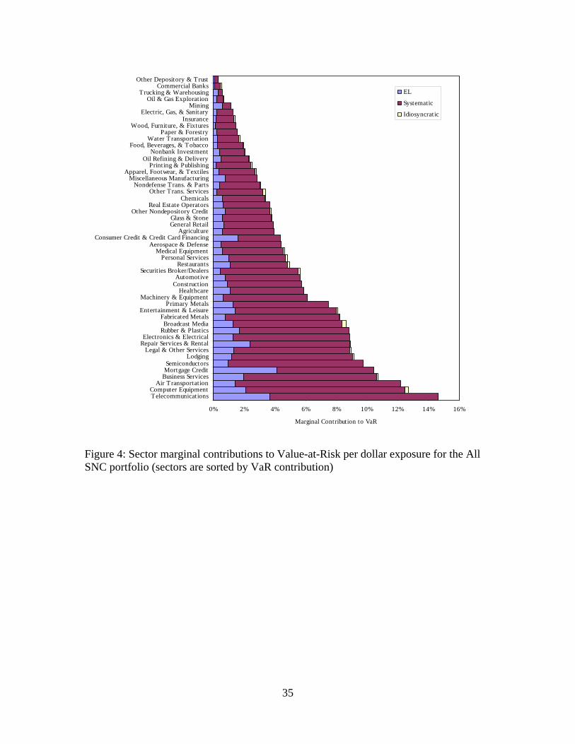
0% 2% 4% 6% 8% 10% 12% 14% 16%

TelecommunicationsComputer Equipment

Air TransportationBusiness ServicesMortgage CreditSemiconductors

LodgingLegal & Other Services

Repair Services & RentalElectronics & Electrical

Rubber & PlasticsBroadcast Media

Fabricated MetalsEntertainment & Leisure

Primary MetalsMachinery & Equipment

HealthcareConstructionAutomotive

Securities Broker/DealersRestaurants

Personal ServicesMedical Equipment

Aerospace & DefenseConsumer Credit & Credit Card Financing

AgricultureGeneral RetailGlass & Stone

Other Nondepository CreditReal Estate Operators

ChemicalsOther Trans. Services

Nondefense Trans. & PartsMiscellaneous Manufacturing

Apparel, Footwear, & TextilesPrinting & Publishing

Oil Refining & DeliveryNonbank Investment

Food, Beverages, & TobaccoWater Transportation

Paper & ForestryWood, Furniture, & Fixtures

InsuranceElectric, Gas, & Sanitary

MiningOil & Gas Exploration

Trucking & WarehousingCommercial Banks

Other Depository & Trust

Marginal Contribution to VaR

EL

Systematic

Idiosyncratic

Figure 4: Sector marginal contributions to Value-at-Risk per dollar exposure for the All SNC portfolio (sectors are sorted by VaR contribution)

35

Automot ive

0.0%

2.0%

4.0%

6.0%

8.0%

All SNC Large Medium Small

P ort folio

VaR

Con

tribu

tion

Systemat ic

EL

Idiosyncrat ic

Const ruct ion

0.0%

2.0%

4.0%

6.0%

8.0%

All SNC Large Medium Small

P ort folio

VaR

Con

tribu

tion

Electric, Gas, & Sanitary

0.0%

0.5%

1.0%

1.5%

2.0%

All SNC Large Medium Small

Portfolio

VaR

Con

tribu

tion

Entert ainment & Leisure

0.0%

2.0%

4.0%

6.0%

8.0%

10.0%

All SNC Large Medium Small

P ort folio

VaR

Con

tribu

tion

Oil & Gas Explorat ion

0.0%

0.2%

0.4%

0.6%

0.8%

1.0%

All SNC Large Medium Small

P ort folio

VaR

Con

tribu

tion

T elecommunications

0.0%

5.0%

10.0%

15.0%

20.0%

All SNC Large Medium Small

Portfolio

VaR

Con

tribu

tion

Figure 5: Marginal contribution to portfolio Value-at-Risk per dollar exposure for selected sectors and portfolios

36