TDA ProgressReport42-111 November15, 1992

The Effects of Correlated Noise in Intra-Complex DSN

Arrays for S-Band Galileo Telemetry Reception

R. J. Dewey

NavigationSystemsSection

A number of the proposals for supporting a Galileo S-band (2.3-GHz) missioninvolve arraying several antennas to maximize the signM-to-noise ratio (and bit rate)

obtainable from a given set of antennas. Arraying is no longer a new idea, having

been used successfully during the Voyager encounters with Uranus and Neptune.

However, arraying for Galileo's tour of Jupiter is complicated by Jupiter's strongradio emission, which produces correlated noise effects. This article discusses the

general problem of correlated noise due to a planet, or other radio source, and applies

the results to the specific case of an array of antennas at the DSN's TidbinbiIla,

Australia, complex (DSS 42, DSS 43, DSS 45, and the yet-to-be built DSS 34).The effects of correlated noise are highly dependent on the specific geometry of

the array and on the spacecraft-planet configuration; in some cases, correlated

noise effects produce an enhancement, rather than a degradation, of the signal-to-noise ratio. For the case considered here--an array of the DSN's Australian

antennas observing Galileo and Jupiter--there are three regimes of interest. If the

spacecraft-planet separation is < 75 aresec, the average effect of correlated noise is

a loss of signal to noise (..0.2 dB as the spacecraft-planet separation approaches

zero). For spacecraft-planet separations >75 arcsec, but <400 arcsec, the effectsof correlated noise cause signal-to-noise variations as large as severed tenths of a

decibel over time scales of hours or changes in spacecraft-planet separation of tens

of arcseconds; however, on average its effects are smaJl ((0.01 dB). When the

spacecraft is more than 400 arcsec from Jupiter (as is the case for about ha][ ofGalileo's tour), correlated noise is a ( O.05-dB effect.

I. Introduction

It is now becoming common practice to array a number

of antennas for telemetry reception in order to increase the

effective aperture [1,2]. The signal-to-noise ratio (SNR)

improvement obtained by arraying is straightforward to

calculate when a pointlike spacecraft is the only source in

the array's field of view. However, the calculation becomes

complicated when an additional hot body (such as a radio-loud planet) is in the beam since, unlike system noise,

the incoming radiation from this hot body is correlated

at different antennas. This article presents a calculation

129

https://ntrs.nasa.gov/search.jsp?R=19930009721 2018-07-13T03:53:43+00:00Z

of the effect of correlated noise on the SNR achieved by a

given array configuration. Other aspects of this topic have

been discussed in [3] and in references therein.

This article is organized as follows: Sections II and III

present a general formulation of the problem, Section IV

considers the special case of an array of N identical anten-nas, and Section V looks at the specific case of arraying the

DSN complex in Australia for Galileo S-band (2.3-GHz)

telemetry reception. To make the article more readable,

many of the detailed calculations have been relegated to

the appendices. Much of the discussion parallels Hjellm-ing's treatment of the Very Large Array (VLA) [4].

II. Outline of the Problem

Consider an array of N (not necessarily identical) an-

tennas. The on-axis gain 1 of the ith antenna is denoted by

Gi and its system temperature (looking at an empty field)is denoted by Ti. The direction toward a point on the sky

can be described by a unit vector _, with s0 pointing to-ward a source at the array's field center. 2 The shape of the

ith antenna beam can be described by the field pattern, 3

a dimensionless function fi(_ - _0) such that f/2(_ _ _0)Gi

describes the effective gain of the /th antenna in a direc-

tion _ - s0 from the beam center. In general, Gi, T/, and

fi may all be elevation dependent. This dependence is not

considered here; it can easily be included in quantitative

calculations. The geometry of the array of N antennascan be described by the set of baseline vectors between

each antenna pair Bit = --Bki, where Bik denotes thevector from the ith antenna to the kth antenna. The basic

geometry is shown in Fig. 1.

It is assumed that the spacecraft is transmitting a

narrow-band, polarized signal with a total Earth-received

power per unit area of 7_,/c and that the planet has a to-tal, unpolarized flux density (power per unit area per unit

bandwidth) Sp. The angular distribution of the planet's

radio emission is described by the brightness distribution

t Throughout this article, an astronomer's definition of antenna gain

is used (commonly measured in units of K per Jy) of G = eA/2kB,

where e is the dimensionless antenna efficiency, A is the physical

antenna area, mad kB is Boltzmann's constant.

:2 Here, s0 is defined as the nominal direction in which the antennas

in the array are pointing, which is the direction assumed when

model delays are calculated (see Appendix A). As discussed in

Appendix C, it is not necessarily the phase center of the array.

3 In general, the field pattern is considered to be a complex quantity

(e.g., [5, p. 27]), but for the purposes of this article, it is sufficient

to assume that it is real.

(flux density per unit solid angle) Ip(_), which is assumedto be constant in time and only slowly varying with fre-

quency (i.e., constant across the observing bandwidth).

Fairly simple assumptions are made about the method

of arraying: The incoming RF signal at the ith antenna is

mixed to baseband, after which a phase shift is inserted.

This phase shift has a component ¢_n (the model phase)

that can be used to compensate, in real time, for phasedifferences between antennas (see Appendices A and C for

details). The baseband signal is delayed by a model delay

vim, and finally, the delayed signals from the N antennas

are summed with appropriate weighting (see Appendix D).It is assumed that the signal is filtered through a rectan-

gular baseband filter of width Au; for an upper sideband

system (which is assumed throughout), the sky frequency

at the center of the passband is u:k _ -- u:o + Au/2, where_qo is the mixer frequency. It is also assumed that the

model delays are chosen so as to compensate for the delay

that a signal from the direction h0 (the field center) suffers

between an arbitrary reference point and the ith antenna.

v/m = ri's___O (1)C

where ri is the vector from the reference point to antenna

i. A simple block diagram of the signal path is shown in

Fig. 2.

The total arrayed power can be written as the sum of

the arrayed power from each of the three sources P_ =p s/e pN where °'/e 19P oN+PP+ _, ._ ,._,._.,represent, respec-tively, the arrayed power from the spacecraft, from theplanet, and from system noise. 4 The effective SNR of the

array is proportional to the ratio of the arrayed space-craft power to the total arrayed power; in the low signal

limit, this reduces to the ratio of P_/c to the power re-

ceived from all sources other than the spacecraft (in thiscase, the planet and system noise). A figure of merit/3 can

be defined for an array; /3 is analogous to G/T for a sin-

gle dish and quantifies how, for a given spacecraft power

(7),/¢) an observing bandwidth (Av), the SNR varies withthe following array configuration:

Au p_l_ Au P_/¢

13 -- 2P,/e P_ _ 27),/c PP q- pg (2)

4 System noise includes receiver noise, sky background, and ground

pickup--all sources of unwanted noise other than individual, iden-

tifiable sources (such as a planet} in the field of view.

130

The term p_/C/ps is the SNR; the term Av/2 p_/C is a

normalization factor that removes from/3 any dependence

on quantities other than array and source geometry.

III. General Expression for 13

As discussed in Appendix A, the summed baseband

voltage can be written in the form

N

v=(_,O= __, Wie-'#"v,(_,t + r_') (3)i=l

where vi(v, t) is the baseband voltage given by Eq. (A-4), v

is the baseband frequency, and Wi is the weighting factor.

The arrayed power is then

(/; /P_ = dvlvm(v,t)l _IT

/ AU N m m 12_:(f ,,,, +r,_ao i=1 I / "_

N N N

:Ew:e,+EEwiwt`_,ki=1 i=l k#i

(4)

where the angle brackets denote time averaging and 7- is

the interval over which the time average is taken; P/is the

single dish power from the ith antenna,

(/; )Pi = dv l,,i(_,,t)l2 (5)

T

and pit, is the unnormalized correlation between the ith

and kth antennas,

spacecraft (P._I_, _le,pit ), the planet (Pi P, p_), and random

noise (P_, p_), so Eq. (4) can be written

N

P_= _ w: (p: '_+ p,_+ P,_)i=l

N N

+__,_ w,w_(p;__+pX+p_)i=1 t`#i

(7)

Thus, Pr., the total power in the arrayed signal, can

be written as the sum of contributions from the three

sources (the spacecraft, the planet, and system noise),

Pr. = P_I* + Ps v + P_, with

N N N

e_'° =_ w:e:'_+_C_C" " -"°,,i,,kVik (8)i=1 i=1 k_i

N N N

P_=_w:P, _+_wiw_p5 (9)i=1 i=l t`_i

N N N

eg = _ w,'e_+F_,_ w,w,p_i=1 i=1 kiki

N

= E W_ P_ (10)

i=1

Because the phases of the individual Pi_ terms in Eq. (10)

are random, their sum is always small (on average, zero)^$/C

and was dropped. However, the sums over p_ and t'ik are

not necessarily small; in fact, a key aspect of arraying is

choosing the inserted model phases to ensure that the sum

over Pi_ is maximized (see Appendix C). Expressions for

P_/_, Pip, and pN are derived in Appendix A, Section II,

and given by Eqs. (A-13), (A-14), and (A-15), respectively.s/e

Expressions for Pik and pP are derived in Appendix A,

Section C, and given by Eqs. (A-25) and (A-28). Substi-

tuting Eqs. (8)-(10) into Eq. (2) gives

• . . %)dv e'(_ -_, )vi(v, t + ry)vT,(v, t + r_ r

(6)

As can be seen in Eqs. (A-11) and (A-18), both Pi and

Pit` can be written as the sum of contributions from the

A/]

13- x2P, I_

N N N

w:P'"/_+ _ E w,w_p:[°i=1 i=I k_i

N N N

Ew,'(e," +p2) + F, Ew, w_pXi=1 i=1 k_i

(11)

131

The phases ul-c_'ik:/¢ and p/_ depend on the quantity 6_bi

6¢/, = ¢i - ¢_n _ Ck + ¢_n, where ¢i,¢k are the actualantenna-based phases, which include both hardware and

atmospheric effects, and ¢_n, ¢_n are the model phases.

If no attempt is made to compensate for the individuals/e

antenna phases (i.e., if ¢_" = ¢_ = 0), the phases of Pik

and pP are uncorrelated from baseline to baseline, and in

both Eqs. (8) and (9) the sums over the cross-correlation

will be small (zero on average). However, as discussed in

Appendix C, the total phase of Plk will be zero for all i, k,

if the values of cm, ¢_ are chosen to satisfy Eq. (C-l):

_/cBik r^= -2_rv w.LS,/¢ - _o]

e

When ¢[n, _b_ are chosen to satisfy the above expression,all the terms in the double sum in Eq. (8) add in phase,

and for large N, the sum over _'i_ contributes signifi-

cantly more to p_/C than does the sum over p._/e (since

pik " PqrPT_Pk). Phases chosen to satisfy Eq. (C-I) max-

imize p_/C, and except in pathological s cases this choicemaximizes /5. The process of determining and inserting

these values of ¢_n, _b_n is referred to as phasing the ar-

ray. In the following, the subscript ¢ is used to denote

expressions that assume that the array is phased on thespacecraft.

Unfortunately, the values of ¢_n, ¢_, which maximize8/e

the sum over Pi_ , may also de-randomize the phases ofpP; as a consequence, sums over pP in Eqs. (4) and (11)

can become significantly nonzero. This is the source of thecorrelated noise contribution from the planet.

Equations (A-13), (A-14), (A-15), (A-25), and (A-28)

can be used to expand Eqs. (8), (9), and (10), and if the

array is phased on the spacecraft [Eq. (C-l) is satisfied],the arrayed power from the spacecraft, the planet, and

system noise can be written, respectively, as

w,w (12)i=1 i=1 k#i

191, : AvkBS1, Wi f_pGii=l

i=1 k_i

N

i=l

(13)

(14)

In the above expressions, )_v, ]k_, represent the average

value of the beam pattern in the direction of the planet,

and _'/_ [defined by Eq. (A-27)] is a dimensionless, complex

quantity, with magnitude less than or equal to unity, which

depends only on the array geometry and the structure of

the planet (or other background source).

By inserting Eqs. (12), (13), and (14) into Eq. (2), the

expression for/3 reduces to

w:a,+ w,w,cVa-, ,c i=l i=1 k#i

Sp 2 t-2

i=1 i=1 k_i i=1

(15)

One can imagine case* where the increase in p_/C obtained by

phasing the array it more than counteracted by the resulting in-

crease in P,EP, but even attempting to array in such cases would be

difficult.

IV. An Array of Identical Antennas

The major effects of correlated noise are easily seen by

examining an array of identical antennas. Consider an ar-

ray of N antennas, e_ch with a gain G, a system tempera-

ture T, and an average field pattern in the direction of the

planet fp. Since the antennas are identical, Wi = 1 for all

132

i. When this array is properly phased on the spacecraft,

Eqs. (12), (13), and (14) become

NG

_¢" -_ f_GSp + T (22)

p S/e¢_ : 2kBN2GPs/c

[i=l

Pff¢ = AvkBNT

and Eq. (15) becomes

NG

N]_GS, I+N-1E E +T/=1 k#i

Since [sP{ < 1 for all baselines, it is always true that

(16)

(17)

N N

1+N-' < N (20)/=1 k_i

From Eq. (A-27) [see also Eqs. (B-I), (B-3), and (B-5)],

it can be seen that, in the limit of an extremely compact

array [i.e., Bik << c/(v_kuRp), for all i,k; Rp being the

characteristic angular radius of the planet], 9rP --_ 1 on allbaselines and

This is equivalent to observing the spacecraft with a single

dish of gain NG and an effective system temperature of

f_GSp + T.

In both cases, the effective gain is NG; it is indepen-

dent of baseline length and depends only on the gains of

the individual antennas. However, the effective system

(18) temperature is not the same in the two extreme configu-rations. The planet contributes Nf_GSp to the systemtemperature in the compact array limit but only ]_GSp

in the extended array limit. In the extended array limit,

the noise contribution from the planet is simply the sum

of its (uncorrelated) contributions to the individual system

(19) temperature. In the compact array limit, its contributionis N times larger due to the correlated noise effects.

Though, as discussed below, the effects of correlatednoise are a complicated function of array geometry. In gen-

eral, the more extended the array configuration, the smallerthe correlated noise contribution of a planet or other hot

body. As a rule of thumb, correlated-noise contributions

are significant on baselines where v_kyBikR,/c _< 1 (seeAppendix A, Section III).

It should be noted that in the intermediate cases where

Bik " C/(ve, kyRp), the sum over _'P may, for some ge-ometries, be negative. In such cases, the performance of

the array is actually enhanced over that of the extended

array limit.

NG

_3¢_°'-* NGSp + T (21)

where the substitution fp : 1, appropriate in this limit, 6

has been made. This is equivalent to observing the space-

craft with a single dish of gain NG and an effective systemtemperature of NGSp +T. Not surprisingly, observing the

spacecraft and planet with a compact array is analogous to

observing the two objects with an antenna with N times

the area of a single array element.

In the limit where Bik >> c/(v_kyRv), for all i,k (i.e.,

an extremely extended array), IJrs[ --- 0 on all baselinesand

6 If the baseline is small compared to c/(vCkRp), the diameters of

the individual antennas would be smaller still.

V. DSN Complexes at S-Band

One of the proposals for support of the Galileo S-band

mission is the arraying of antennas at each DSN com-plex. This section describes the performance of an array

at the Canberra complex that includes DSS 42, 43, 45,and the soon-to-be-built DSS 34. Table 1 lists each an-

tenna, its S-band gain and system temperature at zenith,

its S-band beamwidth at full-width half-power (FWHP),

and its station coordinates (east, north, and vertical) rel-ative to DSS 43.

With the model of Jupiter given in Appendix B, Eq. (15)

can be used to calculate j3¢ for the array. The improvementthat the array would provide relative to the stand-alone

use of DSS 43, if correlated noise effects could be neglected,

is given by the ratio

133

_oo

w:a, + 52w,wki=1 i=1 k_i

_43 N N

s,,F_, a, +F, Wr,i=l i=l

T43 + .f_ap G4aSp (23)X G43

When correlated noise is neglected, this ratio is indepen-dent of hour angle, array geometry, or source structure,

but it depends on Se--the flux of Jupiter--and, there-

fore, on the Earth-Jupiter distance. At opposition, this

distance is 4.2 AU, the S-band flux of Jupiter is approxi-

mately 5.8 Jy and, with the parameters given in Table 1,

/3¢o,//343 = 1.41. At conjunction (an Earth-Jupiter dis-

tance of 6.2 AU), Sp ,m 2.6Jy and fl¢oo/f143 = 1.38. Theimprovement is not as great at large Earth-Jupiter dis-

tances because Jupiter's contribution to the system tem-

perature is less; for comparison, if Sp = O, /3¢oo/fl43 =

1.34. It is useful to note that despite the effects of corre-lated noise, arraying is most useful when extended back-

ground sources are present, particularly if the baselinesare long. In the above calculations, it is assumed that

]e = 1 for all antennas and, as in all the calculations in

this section, Wi = ,¢r_-_/T_ [see Eq. (D-4)]. Throughout

this section, it is also assumed that the gains Gi and sys-

tem temperatures T/ do not vary with elevation, whichleads to a slight overestimate of correlated noise effects atlow elevations.

To assess the effects of correlated noise, the SNK pro-

vided by the actual array is compared with that provided

by the same antennas if arrayed in a configuration with in-

finitely long baselines, examining the ratio/3¢//3¢0 * . Thisratio depends not only on Earth-Jupiter distance, but, in

a complicated way, on the array and source geometriesand on hour angle. Figure 3 plots this ratio for a num-

ber of different geometries. In each plot the declination of

Jupiter, 7 the Earth-Jupiter distance, and the angular sep-

r A declination of -21 (leg, corresponding to that of the Galileo en-

counter in December 1995, has been used for Fig. 3. The results for

other Jupiter declinations are different in detail but qualitativelyvery similar.

aration between the spacecraft and the center of Jupiterare held fixed. Each point on the plot then represents

the value of/3¢//3¢0* for a randomly chosen value of the

hour angle, the orientation on the sky of Jupiter's radi-

ation belts, and the orientation of the spacecraft-Jupiter

separation. Thus, the density of points on a portion of aplot provides an estimate of the likelihood, as a function of

the hour angle, of obtaining a particular value of/3¢//3¢00for the given parameters.

Figures 4(a) and (b) summarize the results of the

calculations shown in Fig. 3 plotting, as a function of

spacecraft-Jupiter separation, the average (over hour an-

gle and orientation) value of/3¢/fl¢0., as well as its min-imum and maximum values. Thus, each plot in Fig. 3 is

reduced to three points in Fig. 4--one on an average curve,

one on a maximum curve, and one on a minimum curve.

The following conclusions can be drawn from Fig. 4:

(1) When Galileo is within --_75 arcsec of Jupiter, the

average effect of correlated noise is a loss of SNR,which may be as large as 5 percent at zero separa-tion.

(2) When Galileo is more than 400 arcsec from Jupiter,

the effects of correlated noise are negligible.

(3) For separations in the range of 75 to 400 arcsec, the

effects of correlated noise are small on average. How-

ever, the loss may be significant for certain geome-tries (as may be the enhancement). In this range ofplanet-spacecraft separations, careful calculations of

correlated noise are necessary in a case where a 5-percent SNR loss would be critical.

The above conclusions refer specifically to an array con-sisting of the antennas listed in Table 1. Correlated noise

effects are likely to be similar for arrays of similar antennas

with similar baseline geometries, but quantitative calcula-tions for other arrays have not been carried out. Because

correlated noise causes significant SNR variations, and be-

cause these variations are highly geometry dependent, de-

tailed calculations of these effects should be done for anysituations in which a few tenths of a decibel of SNR are

crucial. For most purposes involving Galileo and Jupiter,

Eqs. (15), (8-6), and (B-9) should be suitable for suchcalculations.

134

Acknowledgments

Many thanks to George Resch for numerous informative discussions of interfer-

ometry, reading the early drafts of this article, and help with Figs. 1 and 2; and toJim Ulvestad for his careful refereeing of the article.

135

Table 1. S-band parameters of antennas in proposed Canberra array.

Antenna Gain, System S-broad beamwidthK/Jy temperature, K (FWHM), deg

Station coordinates _

East, m North, m Vertical, m

DSS 43 0.95

DSS 42 0.21

DSS 45 0.16

DSS 34 b 0.16

18.5 0.11

22.0 0.28

38.0 0.23

30.0 0.23

0.0 0.0 0.0

0.0003 194.1921 -13.6414

-325.3907 440.1822 -13.1378

68.8 440.2 0.0

Relative to DSS 43.

b Values for DSS 34 are approximate.

136

_NAVEFRONT FROM A

SOURCE IN DIRECTION- 4

ANTENNAS POINTED _-... /" )lK

"_\ / _",. INDIRECTION_ "._ //

-- _ ,... -.o.. y,/

jrANTENNA i / ANTENNA k

ARRAY

REFERENCEPOINT

Fig. 1. The basic geometry ot an array. Antennas I and k are lo-

cated at, respectively, ri and rk with respect to the array reference

point and are pointed toward the direction -_0. It Is clear from the

diagram that the delay suffered by a wavefront from a direction ._

between antenna i and antenna k is proportional to Bik • _.

i DELAY

PHASE SHIFT

t

LOCAL OSCILLATORvio

PHASE SHIFT

2.,-W/o "tm + * _

I DELAY_ _0"_;-_'-

i

ADDERTO

._-.-=--TELEMETRY

EQUIPMENT

Fig. 2. A simplified block diagram of an array signal path.

137

1.2

Q:" 1.0

aQ.

0.8

1.2

_- 1.0

0.8

1.2

1.0

' ' _ ' t ' ' ' ' l ' _ ' r F ' ' ' '

EARTH-JUPITER DISTANCE: 4.2 AU

JUPITER-SPACECRAFT SEPARATION: 10.0 arcsec

AVERAGE _,¢/_¢= = 0.97

MINIMUM _¢/_,_ = 0.95

MAXIMUM _,¢/_¢® = 0.99

i = i r I t i i i t i J = = I i i L r

' ' ' ' I ' _ ' ' I ' ' ' ' I ' ' _ P

EAR_UPITER DISTANCE: 4.2 AU

JUPITER_SPACECRAFT SEPARATION: 100.0 arcsec

AVERAGE p$/_$® = 1.00

MINIMUM _¢/_$® = 0.96

MAXIMUM I_/1_,== 1.o3

' ' ' ' I ' ' _ ' I ' _ ' ' I ' ' _ '

EARTH-JUPITER DISTANCE: 4.2 AU

JUPITER-SPACECRAFT SEPARATION: 300.0 arcsec

AVERAGE _$/_$= = 1.00

MINIMUM _$/_$= = 0.98

MAXIMUM i55/_,#_,:= 1.01

1.2, ' ' ' ' I ' ' ' ' i ' ' ' _ I ' ' _ '

EARTH-JUPITER DISTANCE: 4.2 AU

JUPITER-SPACECRAFT SEPARATION: 500.0 arcsec

EARTH-JUPITER DISTANCE: 6.2 AU

JUPITER-SPACECRAFT SEPARATION: 10.0 arcsec

AVERAGE _,_/_,$,®= 0.98

MINIMUM _$/_,_= = 0.97

MAXIMUM I_/l%#® = 0.99

i t i = I i i , i I i i i i t = i t

' _ ' _ I ' ' ' _ I ' ' _ ' t ' ' ' '

EARTH-JUPITER DISTANCE: 6.2 AU

JUPITER-SPACECRAFT SEPARATION: 100.0 arcsec

AVERAGE I_p$= = 1.00

MINIMUM _$/_$® = 0.97

MAXIMUM p_'p_,== 1.o2i J i , J i I , ; I I I , , i = i I =

EARTH-JUPITER DISTANCE: 6.2 AU

JUPITER-SPACECRAFT SEPARATION: 300.0 arcsec

____.._ _-..,z_•

AVERAGE _$/1_ = 1.00

MINIMUM _/_¢_o = 0.99

MAXIMUM I_$/_$= = 1.01

' ' ' ' t ' ' ' ' I .... I ' ' ' '

EARTH-JUPITER DISTANCE: 6.2 AU

JUPITER-SPACECRAFT SEPARATION: 500.0 arcsec

AVERAGE I_¢/1_¢®= 1.00

MINIMUM p¢/_® = 1.00

MAXIMUM _$® = 1.00

-5 0 50.8

-10 10 -10 10

AVERAGE _$oo = 1.00

MINIMUM I_$/[]_= = 1.00

MAXIMUM _#_$oo = 1.00

-5 0 5

HOUR ANGLE, hr

Rg. 3. The raUo of/_,///_c_ for an array of antennas at the DSN Canberra complex observing Jupiter and a spacecraft at S-band,

for a variety of array and source geometries. The declination of Jupiter = -21.0 deg and the array consists of DSS 43, DSS 42,

DSS 45, and DSS 34.

138

1.10 [ ..... " " " " ' .... ' ..... ' .... r ' r ' ' ..... ' '

f (a)

1.05 [ (_/_*®)max

1.00 [ _ -. ....

0.95

0.90 L .......... , .... ' ................

1.10 [ .... ' .... ' ..... ' .... " " ' " ' .... ' ..... ' "

(b)

1.05

_- 1.00

(_/_$_) max

J

0.95

0.90 ......... , .....0 100 2oo aoo ,,00 500 600

JUPITER-SPACECRAFT SEPARATION, arcsec

k , ,

700

Fig. 4. The average, minimum, and maximum values of _//J34,ooobtained as source orientation Is varied, plotted as s function of

the separation between the spacecraft and the center of Jupiter,

with Jupiter declination = -21.0 deg: (a) Earth-Jupiter distance =

4.2 AU and (b) Earth-Jupiter distance = 6.2 AU.

139

Appendix A

Basic Expressions

I. Incoming Signals

The voltage (as a function of time t and sky frequency _,kv) induced in a single polarization channel at ri, the focal

point of the ith antenna, by a distant s source (e.g., a planet or spacecraft) can be written

v_(.,k_,t) = e_' _ ff a_/i(_ - _o)Z(.._y,t, _)ei(2"".k.[t - (_.rJe)] + 0(-.k,, _)) (A-l)

In this expression, kB represents Boltzmann's constant and c is the speed of light; Gi is the on-axis antenna gain, fi

is the magnitude of the antenna's field pattern, h is a unit vector in the direction of the source, Z(_'_ky,t,_) is theamplitude of the electric field due to the source, 0(t'sky, _) is a phase term (which for most astronomical sources can be

assumed to be uncorrelated over _0_ and _), and ¢i is an antenna-based phase shift (including atmospheric effects).

The voltage induced by system noise can be written

v,"(.,_.,t) = k_/T_.V,ei (2..,,,t + C(_._,0) (A-2)

where Ti is the noise temperature and Off(v,k_,t) is a random phase that is uncorrelated over time and frequencyintervals satisfying Av, kyAt > 1. The total RF voltage can be written as the sum of terms due to the spacecraft,planet, and system noise:

(A-3)

When the RF signal is mixed to baseband, it is phase shifted by 21r14orim; this stops the fringes, allowing time averagingover a longer interval. An additional phase shift -¢7' can be inserted to (attempt to) compensate for the antenna-basedphase shifts ¢i. Without this additional phase shift, the baseband voltage can be written

vi(i_, t) = ei2Xv'°r,me-i2"v'-'_(/2sky, t)

-- ei2"V'o[rff-'] [ViS/c(_sk,, 71)+ "liP (l,'sky,t) 4- ViN (l/,ky,t)]

= ff - ')

4- Zp(l/sky, t, §)e ieP(u'k,'a)] 4- ei2Xv'°tr_'-t]kv/_iBTiei(2_u°kvt+_(v'_'t))

+ Zp(_,,_, t, h)ei*'(,'','_)] + kV/_-_ ei(_*t'*+"o'.']+_._('.,,,O) (A-4)

s Here, "distant" means a source sufficiently far away that, over the extent of the array, a plane wave approximation is valid.

140

where u = v, kv - U_o is the baseband frequency. Like the RF voltage, the baseband voltage can be written as the sumof terms due to the spacecraft, planet, and system noise:

vi(,,,t) = v:/_O,,O + vf(v, 0 + o_(v,t) (A-5)

If the additional phase shift is inserted, the baseband signal has the form e-i¢?vi(v,t).

II. Single-Dish Power

For the ith antenna, the single-dish power can be written

= d_Ivi'/°(_,t) + ._(_, t) + ,y(_, t)l_T

= dr, [v_ t _, r)v_ t_, t) + " + t)v i t v, t)

sic P+ v i (v,t)v i *(_.,t) + viP(.,t)vP*(_.,t) + vN(_',t)vP*(_',t)

T

where the angle brackets denote a time average and T is the interval over which the time average is taken. Looking at

each term separately and considering the planet term first,

._(_, t)v_"(., t) = e_' _ g d_/_(_- _o)e_2"(_t'-(i"/°_l+_'°t':_-(_"/')l_ZeO"+ ",o,t, _)e'°"(_+_'o'_

e-J" f f d_' fi(s' - So)e-i2r(_'[t-(iJ"ri/e)]+u'°[r'*-(i"rJc)])ZP( b' q- lJlo, t, _/)e -iae(_+v'°'i')x

= kBC, i g d§ fi(s - §o):Ip(l/ W l]lo,t,') _ d§' {e -i(2"(_'['-a']r'+t''°['-'']r')]c)

x d[°"(_+"'o,_)-°_(_+_'o,i')]f_(s ' - s0)Zp(_, + _,lo,t, s')'_)

= kBGi//

= kB Gi f� d_y,_(_- _0)_(. + ._o,_,_) (A-7)

141

where the integralover i'isnonzero only when _'= i because the radiationfrom the planet isspatiallyincoherent,

and where the substitution77_(v+ vzo,t,_) = Ip(_ + Vto,t,§) was made; Ip isthe brightnessdistribution(fluxper unitsolidangle)of the planet.Similarly

vi (u,t)v i (_',t)=keGi d_fi2(h-_o)l,l,(U+_o,t,_) (A-S)

with I_1 c being the brightness distribution of the spacecraft (usually assumed to be pointlike), and

viN (u, t)vi N'° (u, t) = kvTi (A-9)

Compared to these terms, the cross terms are all small, as can be seen by considering

v_l'(u,t)viP*(_',t) = kBGi d_ fi(s-_o)Z, ic(u+u_o,t,_ ) JJP d_' {e ,(2,,/c)(_,[..'It +,,,.[s .'],-,)

ei[O'le(u+Ulo,_)-OP (v+ulo,il)] fi(_t _o)Ip(u + uto,t, _') }X

0 (A-a0)

where the integralover g'issmall because 0"/_and 0e are uncorrelated[unlikein Eqs. (A-7) and (A-8),thisintegralis, on average, zero, even when _' = §].

One can therefore write

= du Iv_/'O,,t)l _ + Ivff(t,,t)l z + Iv_(v,t)l _/T

= P;/" + PP + PiN (A-11)

It is assumed that the spacecraft is a point source located at is/c, transmitting a narrowband, polarized signal at a

sky frequency _/_ with a total power Ps/c. The brightness distribution seen by a receiver matched to the signal's

polarization 9 is

I,l_(U_ku,t,h) = 2P,/_ (u_ku$/c_

- -ok_)_(_- _,/o) (A-12)

(with 6 representing a Dirac delta function), so

0The factor of 2 in Eq. (A-12) arises from the assumption of matched polarizations.

142

p:/C = 2kBfi2(_8/c _ _o)GiP,/c ,_, 2kBGi'P,,/c (A-13)

where it is assumed that f_(_8/c - _0) _ 1 (i.e., the spacecraft is close to center of the array's field of view).

It is assumed that the planet is an extended, unpolarized, broadband source of total flux at the frequencies of interest

of Sp, which is constant in time and varies only slowly with frequency (i.e., it can be considered constant across the

observing bandwidth Av), so Ip(vjk_,l, _) = Ip(_) and

Pie= kBGiAz; ff,.d = a,,',,,s,. (A-14)

where f_.,, is a weighted average of fi2p over the planet.

Finally, from Eq. (A-9)

P,_ = ksT_a_ (A-15)

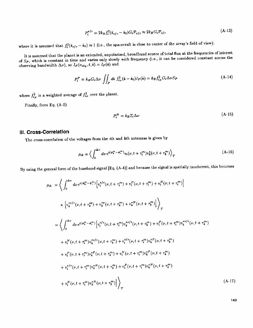
III. Cross-Correlation

The cross-correlation of the voltages from the ith and kth antennas is given by

pi,, = dye ¢_',-_', _v,(,.,,t+ .y)vi(,.,t + "7) (A-16)T

By using the general form of the baseband signal [Eq. (A-4)] and because the signal is spatially incoherent, this becomes

0,_ = a.e_(+r-+r) _/°(.,t+.gl+vg(.,t+ry)+v_(.,t+_y)

[ *sic, t *Px [v_ t_', +-_)+vk (',t+_'_')+_Tv(_',t+'_)]I '7"

(foZX_'db, e/(¢__CT)[ sic m_, *s/c, . m', *s/c, .= ,,_ (_,,t+,_)v_ t,,,_+,_')+,,_(_,,t+-_ jv_ t_',_+,_)

+_,_(,..,t+._ ),,,, _,..,t+._')+ + +,-_)

+ .i t-,t + _ _ k , , + .;') + + ._)v;_(_, t

+ v_(u,t + _ s _ t, + r_") (A-17)7-

143

This can be written as

where

Pik _ Pik (A-18)

<_o av • " _ m, ,,/¢, t+r_n)> (A-19)_/_ dye '(¢k -¢' )v_/C(v,t + ri )v k iv,Pik =

T

pP = dye (_k ¢')v i (v,t+v i )vkv(v,t+r_" ) (A-20)

T

pN = d.e_(_.r-., '') v_(v,t+rg,)v;g(v,t+r,T)+vP(v,t+ry)v'k./_(v,t+r_)

rnx *s/c1 . $/c_ .+v,_(.,t+r, )v_ t.,,,+_-_')+v, _.,,+.l")v:(.,t+.?)

+ ,,,_(,,,t+ .r)viP(_,_ + .r) + _:/'(.,_ + -?),;_(_,_ + _r)

+ v_(v, t + r/n)v;N(v, t + _-_)] > (A-21)T

These expressions are similar in structure to the expression for single-dish power [Eq. (A-6)]. Looking at pP, one finds

viV(y,, + r_)v,P(y,t + rr)= e'("-*')kB Gv/-G-_IG_ei2"[p+_'*l[ry-'T] [ff d§{e-i(2"l"+v"li'r'/e)fi(§-'o)Ip(')

x// - )]d_' fk(§' -- §o)Ze(s')e i(2"[u+u'o]i''r"le)ei(#'("+v'* s) or'(.+.,., s'))

(A-22)

144

where the substitutions r/'n = §o.ri/c, r_ n = so.rk/c and Bik = rk -- rl have been made.

Similarly

v:/_(_,t + ,y)v;'/_(_, t + ,;") = e'(_'-")kBv_,a_

f/d§ ei(2_[v+u'°][i-i°]'B'h/e)f/(§ -- §0)h(s -- so)/,/¢(s) (A-23)×

In considering the effects of noise, it is assumed 1° that Eq. (A-21) can be approximated as

_, kB T_._iTkl f °zx, dye i(¢_'-¢7') ei(2,_[t+_gl+2,_V, or,"+o_(_,_,t+_:")) e -i(2,_[¢+r2]+2_V, or_'+o_(_.k_ '_+_;")117"1

_-. cBVli_kTe ,"

kBT_/_-_'_T__/-_e _ (A-24)

where 0_ is a phase randomly distributed between 0 and 27r, and where use has been made of the fact that 0ff(v,k_, t)

is uncorrelated between antennas and over time and frequency intervals where At,'/" > 1. Because the phases of pit_ are

random, the double sum in Eq. (I0) will be small. However, as discussed in Appendix C, noise terms become importantwhen the process of phasing the array is considered.

Using Eq. (A-12) to substitute for I_/_,

(/0sir i " " i -Plk 2"Psi, dvS(v -_ s/_ _ Vto])e (¢* -¢' )e (_' ¢_)k/3_.= Ll_sky

x ff oln( - -

= 2PslckB GV/-_iG_ei(_¢,-_¢*)ei(_'rv;_[i'/'-i°]'B'k/e)fi(_,l ¢ _ ,3o)fk(,3,l _ - ,3o) (A-ZS)

_0 This assumption is not vMid if the planet or the spacecraft contributes significantly to the system temperature; in that case, the cross

terms in Eq. (A-21) will be non-negllgible. However, they can be treated in a manner similar to the vNv * N term.

145

$/c r^Note that s,/c- s0 must be small enough that the quantity v, tulS,/c -_0]-Bik/c does not change significantly over theinterval of the time averaging.

Similarly,

(// : $pP = kB_e i(64_'-64_'1 di fi(i - io)fk(i - io)Ip(i) dye i(2"[u+u'ol[i-i°lB'k/c)

IT

At this point, it is useful to define the quantity

(A-26)

so that

H If"1 d_ ei(2"_'°n'*'(i-i°)/c)fi(_ - s0)fk(_ - s0)Ip(h) due i(:"'B'*(a-i°)/c)"TP = AuSp (A-27)

Pi_ = AvkBSt" Gv/-G_iG_ei(6*'-6_k).Ti_ (A-2S)

.TP is a dimensionless complex quantity that depends only on the array geometry and the source structure and whose

magnitude is always less than or equal to unity (]-_'_1 --' 1 in the short baseline limit, and I_/_l --+ 0 in the long baselinelimit).

It has been implicitly assumed that the bandpass is rectangular, in which case the integral over u can be simplified:

foAV d_, eiOXura,_.(i-io)/C) = ei(,zx_,n,h.li-io]/C)sinc ( _ Bik.[_ _ §o]) (A-29)

where sinc(x) = sin(xx)/lrx. This term, often referred to as the delay beam, introduces a phase shift and lowers the

correlation amplitude for _ _ ,_0; both these effects are more pronounced for larger bandwidths Av.

One can therefore write

"TP - AvSp1 i/ d§ e*(2_'o',B"(s-'°)/e)fi(h"" " " " --/0)/k(s --/0)Ip(/) sine (-_--Bit-[s -10])Au ^ (A-30)

where c AvI2.I,]sky .._ 1,tlo -._

If the quantities fi, fk and sinc(AuBik.[_ - fi0]/c) do not vary greatly over the extent of the planet, one can makethe further simplification

fi _i(2,_,_k. n,h.(i-lo)/c) r :-'_1 .]ipfkpfAuik ds _ • iptB) (A-31)•_S- AvSe

where _p, j_p, ]a, ,k are suitably weighted averages of fl, fk and sinc(AvBik-[h - h0]/c), respectively.

146

Appendix B

Jupiter Model

At centimeter wavelengths, Jupiter is not a simple thermal disk; there is significant synchrotron emission from the

radiation belts and the resulting flux distribution is quite complicated [6,7]. For the purposes of this article, Jupiter

can be modelled as the sum of three components: two circular (2-dimensional) Gaussian components (representing the

radiation belts) and a uniform central disk. This is a simple model to work with because Eq. (A-27) can be integrated

analytically for each of these components.

If the brightness distribution of a source is radially symmetric about the point sc, small compared to the delay

beam, and small compared to the primary beam of any antenna, Eq. (A-27) can be written

/52fifk ]a,,k e,(2_v_,_,n,_ [,c ,0]/0 r dr I(r)Jo (B-l)

where r = I_ - sol; ]av,k is the value of the delay beam at the source; fi, fk are the average vMues of the antenna;

field pattern at the source; for the ith and kth antenna; S is the total flux of the source; I(r) is the source's radially

symmetric brightness distribution; and J0 is a zeroth-order Bessel function.

For a uniform disk of angular radius RD centered at sc,

S

I(r) = 7rR_ r < RD

= 0 r > RD (B-2)

_D = ]ih]au,k ei(2,v_.k,le)n,k.(iO--_o) eJ,(2r_:_uBikRD/c) (B-3)7ru_kyBi_ RD

For a circular Gaussian of total flux S and characteristic size (1/e radius) Re, centered at so,

I(r) = _ -r2/R_ (B-4)_rR_ e

and Eq. (B-I) becomes

::_ = J,J*J_,k _¢'t"¢. oi(2""_,k_B,k'[_c-_o]/_)e--(_2k'B'ka°/e)= (B-5)

Jupiter's brightness distribution is modelled as the sum of a uniform central disk of radius R j, centered at §I, andtwo circular Gaussians of characteristic size RB, representing the radiation belts, which are offset from the center of

the disk by =kAsB. The flux of the central disk is written as FDSs, where Sj is the total flux of Jupiter and FD is the

fraction of that flux in the disk; the integrated flux of each wing component can be written as (1 - FD)SS/2. Using

this model with Eqs. (B-3) and (B-5),

147

cos\--7- (B-6)

If the above expression and Eq. (C-l), the condition that the array is properly phased on the spacecraft, are substituted

into Eq. (A-28), one gets, for the cross-correlation due to Jupiter in a phased array,

r cJl(2rv_kvBikRj/c) _ . e-('v_k, B'''nBle)_

× [FD _ +(1-- /_O) 7r

In the case where S,lc s0 and/or ale c= vjk v = v_kv, this simplifies to

_J _J ?J _i(2r,v',ch_Bik .[ij-'_,/c]/c)P:k = AvkBSJV_k Ji J_ _,k _

CJl(27rv_kyBikRj/c) e--(TV._k,B'"RB/C)_x FD 7r " • +(1--FD)v.,kv B,k. R.j

:-.:,, )]cos (x_Bik "ASB

/ 27rv,_k_ _ 1

cos _,_B,,.AsB)J

(B-7)

(B-S)

Both the total flux Sj and the flux distribution are functions of frequency and Earth-Jupiter distance. From the data

given in [5], the model at S-band (2.3 GHz) used in this article is

Sj = 6.3 (4'0dAU)2-- Jy

FD =0.3

4.04 AURj = 24.3 -- arcsec

d

(B-9)

At conjunction, d = 6.2 AU, S_ = 2.7 Jy, and R$ = 15.8 arcsec; at opposition, d = 4.2 AU, Sj = 5.8 Jy, andRj = 23.4 arcsec.

Figure B-l(a) shows a map of Jupiter from [6] at 2.9 GHz (10.4 cm), while Fig. B-l(b) shows a higher resolution

map from [7] at 1.4 GHz. Note that in Fig. B-l(b), the disk has not been removed. Figure (B-2) shows the model of

Jupiter used in this article in the same format as Fig. B-l(a).

Z

<

1 i

- (a)

0

1 i I I , , I I I I , ,2 1

/

JT OK= ........ .--

0 1 2

ARCMIN

(.,)uJ0_oE<

40--

30--

20--

10--

0

-10 --

-20 --

-,30-

-40-

I(b)

I I I

I I I

I I I I -

1 Rj

I ::::' I ¢' I "_" ':_'1 I80 60 40 20 0 -20 -40 -60 -80

ARCSEC

Fig. B-1. A map of the brightness distribution of Jupiter: (a) at 2.9 GHz with a 260-K diskcomponent removed and 20-K contour intervals (from [6]) and (b) at 1.4 GHz, Including diskcomponent with contour Intervals at 2, 5, 10, 20, 30, 35, 40, 50, 60, 70, 80, and 90 percent (from[7]).

Z

On-',<

1.0

0.5

0

-0.5

-1.0 t

-2

.... ..._ ......... ..._ , '..-- ...... _....." , , , ,"'" "- "- CONTOUR

/" _ "" ..... _ "\ INTERVAL =

,// T= 20 K "\ 20 K

• - Kj =

L .t T O =260 K ...."i i "'"r- • -,|_" i i A I

-1 0 1 2

ARCMIN

Fig. B-2. A model of Jupiter's brightness distribution at S-band [see Eq. (B-9)], plotted In thesame format as Fig. B-l(a) with disk component removed.

149

Appendix C

Phasing

I. The Ideal Case

The SNR on the spacecraft is maximized when the

terms in the double sum in Eq. (8) add in phase. This can

be (approximately) arranged with the appropriate choice

of model phases ¢_. By using Eq. (A-25), ,/e_qk will havezero phase for all i, k when

6¢k - 6¢, = ¢k - ¢7 - ¢, + ¢7's/c

_¢Vaky

= _Bi_.(_°lc - _o)C

(c-1)

The above relation can be satisfied if, for all i = 1, ...N,

The phase ¢_'j, of the correlation function is given by

tan _'k - Im(pik)Re(v,_)

a/c_ Im(p,_ ) + Im(p P) + Im(p N)

_tetp_k ) + Re(p P) + Re(p_)(c-3)

where Re and Im represent, respectively, the real and

imaginary parts of the complex function. The simplest

phasing algorithms make the approximation that the

spacecraft signal is the dominant contribution to Pik, i.e.,

s/c

"Irl/aky

¢7' = ¢, + --s+,. (_,/o - _0) (c-2)C

tan_k _ Im(pik) .._ Im'pikC't°/_ (C-4)Re(pi_) _ " , ,/e,tte(Pi_ )

where r represents an arbitrarily chosen reference antenna.

The values of ¢i are not known a priori, but there are

N(N- 1)/2 independent measurements of the phase of thecorrelation function that can be used to fit for the N model

phases ¢_ (see [8]). Note that since 6¢i , 6¢, include media

effects as well as phase shifts in each antenna's signal path,they vary on timescales of seconds to minutes, so that the

model phases must be recalculated at least that frequentlyto prevent degradation of the signal.

This approximation requires that lp_._/cl>> IpPI andp't¢l

i_ I >> IP_I for all baselines Bik. Using Eqs. (A-24),(A-25),and (A-28),thisimplies

mtJSp ¢.p (c-5)

and

II. The Effects of Random Noise and aBackground Planet

The above discussion ignores the contributions of ran-

dom noise and a background planet to the observed phases.These complicate the process of solving for model phases,

since what actually can be observed is the phase of the

total correlation Plt, not the phase _,,/_it , the correlationdue to the spacecraft signal.

_',/, >> 7 (c-6)

In theory, the first of these conditions can be circumvented

by modelling the contribution of pP to the phase of Pikin the phasing algorithm. The second condition is more

fundamental and can only be dealt with by decreasing theobserving bandwidth (if the spacecraft is a narrowbandsource) or increasing the time over which the correlation

is averaged.

150

Appendix D

Weighting Factors

The weighting factors Wi should be chosen so as to maximize t3¢, which is given by Eq. (15). Such Wi will satisfythe condition

d/_.__._.¢= 0 (D-l)dW_

for all j = 1, ...N. Since one of the weighting factors can be chosen arbitrarily, this condition amounts to N - 1

equations for N - 1 variables.

If the effects of the planet can be ignored (i.e., fit, _ 0), Eq. (15) reduces to

w:e, +ZZw, wki=1 i=1 k#_ (D-2)fl_b: N

i=1

and Eq. (D-l) becomes

It is not terribly difficult to show that this is satisfied for

v_7w,.: -97-, (D-4)

If the contribution of the planet to the system temperature at each antenna is accounted for, but the correlated

noise terms are ignored, the optimal weighting is

This is appropriate for an extremely extended array. If correlated noise terms are included, it is difficult (perhaps

impossible) to solve for W/ in closed form, but it can be done numerically. For the array configuration at the DSNcomplex in Australia, the weights obtained, including the effects of correlated noise, differ by only a few percent from

those given by Eq. (D-5), and they have a negligible effect (<0.5 percent) on the values of tiC. In fact, though thevalues of Wi obtained, including the effects of correlated noise, often differ by --_10 percent from those obtained from

Eq. (D-4), the resulting values of fie differ by <1 percent. Therefore, throughout this article, Eq. (D-4) is used to

calculate weighting factors.

151

References

[1] R. Stevens, "Applications of Telemetry Arraying in the DSN," TDA Progress Re-

port _2-72, vol. October-December 1982, Jet Propulsion Laboratory, Pasadena,California, pp. 78-82, February 15, 1983.

[2] D. W. Brown, W. D. Brundage, J. S. Ulvestad, S. S. Kent, and K. P. Bartos, "In-

teragency Telemetry Arraying for Voyager-Neptune Encounter," TDA Progress

Report _2-102, vol. April-June 1990, Jet Propulsion Laboratory, Pasadena, Cal-ifornia, pp. 91-118, August 15, 1990.

[3] M. It. Brockman, '°The Effect of Partial Coherence in Receiving System Noise

Temperature on Array Gain for Telemetry and Radio Frequency Carrier Recep-tion for Receiving Systems with Unequal Predetection Signal-to-Noise Ratios,"

TDA Progress Report 42-72, vol. October-December 1982, Jet Propulsion Lab-

oratory, Pasadena, California, pp. 91-118, February 15, 1983.

[4] R. M. Hjellming, ed., An Introduction to the NRAO Very Large National RadioAstronomy Observatory, Socorro, New Mexico, 1983.

[5] W. N. Christiansen and J. A. Hogbom, Radio Telescopes, New York: CambridgeUniversity Press, 1985.

[6] G. L. Berge and S. Gulkis, "Earth-Based Observations of Jupiter: Millimeter to

Meter Wavelengths," in Jupiter, T. Geherls, ed., Tucson: University of ArizonaPress, pp. 621-691, 1976.

[7] I. de Pater, "Radio Images of Jupiter's Synchrotron Radiation at 6, 20 and

90 cm," Astronomical Journal, vol. 102, pp. 795-805, August 1991.

[8] J. S. Ulvestad, "Phasing the Antennas of the Very Large Array for Reception

of Telemetry From Voyager 2 at Neptune Encounter," TDA Progress Report

42-94, vol. April-June 1988, Jet Propulsion Laboratory, Pasadena, California,pp. 257-267, August 15, 1988.

152