the effects of animal grazing on the multiple …

THE EFFECTS OF ANIMAL GRAZING ON THE MULTIPLECOEXISTENCE AND DIVERSITY OF PLANT SPECIES INGRASSLAND COMMUNITIES

著者 Pulungan Muhammad Almaududiyear 2020-06出版者静岡大学URL http://doi.org/10.14945/00027794

THESIS

THE EFFECTS OF ANIMAL GRAZING ON THE

MULTIPLE COEXISTENCE AND DIVERSITY OF

PLANT SPECIES IN GRASSLAND

COMMUNITIES

June 2020

Shizuoka University

Graduate School of Science and Technology,

Educational Division

Department of Environment and Energy Systems

Muhammad Almaududi Pulungan

THESIS

THE EFFECTS OF ANIMAL GRAZING ON THE

MULTIPLE COEXISTENCE AND DIVERSITY OF

PLANT SPECIES IN GRASSLAND

COMMUNITIES

草原群落における植物種の多種共存・多様性に及

ぼす動物による採餌の効果

2020年 6月

静岡大学

大学院自然科学系教育部

環境・エネルギーシステム専攻

ムハッマドアルマウドゥディプルンアン

Abstract

Grasslands are perfect examples for plant communities with extremely high species

diversity. Many studies have reported that the species richness of grassland is one of the

highest among plant communities in the world. In fact, some grasslands win out over tropical

forests in terms of diversity on a small scale. By comparison, a small area of grassland can

contain more species than that of tropical forests. Occupying one-quarter of the Earth's land

area, grasslands become a vital part of the world's ecosystem. The loss of biodiversity from

grassland communities may be damaging both the good and services of the ecosystem on

which the human population depend. Therefore, preserving grassland's diversity is essential

to maintain the ecosystem's processes.

Grazing is an important process in grasslands. In natural, seminatural, and managed

grasslands, animal grazers play a significant role in regulating diversity. Extremely high

grazing intensity converts grassland to bare land intensively which in turn reduces the

diversity. In grassland studies, an intermediate level of grazing often results in the highest

species diversity. However, why and how an increase in grazing to a certain point increases

the diversity remains an open question.

A few studies have proposed hypotheses to explain this counterintuitive phenomenon,

such as a tradeoff of growth and mortality between species. However, so far, we have no

convincing theory to explain this unimodal response of species diversity to grazing intensity

at an intermediate level. Models built by scientists tend to be limited in representing the

existence of a single or a few dominant species. Using these models would be very difficult

in modeling the present species diversity. Here, we present a simple model to explain the

rich diversity in grasslands. We build a lattice model of a grassland community comprising

multiple species with various levels of grazing. We develop a two-layer lattice model, adding

another two-dimensional lattice of grazers that randomly feed on plants. We investigate the

effect of grazing in two cases, i.e., tradeoff case and opposite case, which differ in species

dependence of grazing mortality. This study also explores the effect of grazing intensity on

the species composition. In addition, we examine the effect of varying the dispersal rate and

lattice size.

We then analyze the relationship between grazing and plant diversity in grasslands under

variable intensities of grazing pressure. The highest species diversity is observed at an

intermediate grazing intensity. Grazers suppress domination by the most superior species in

birth rate, resulting in the coexistence of inferior species. The coexistence of species is

mechanically promoted because (weak) grazing produces vacant sites available for other

species. The positive correlation of birth rate and grazing rate (tradeoff case) promotes

coexistence better than a negative correlation (the opposite case). However, the tradeoff is

not necessary for the unimodal variation of species diversity as grazing intensity increases

because the unimodality is observed in both cases. The positive and negative correlation

between grazing and growth rate influences the composition of species. The unimodal

grazing effect disappears with the introduction of a small amount of nongrazing natural

mortality. Thus, unimodal patterns of species diversity may be limited to the case where

grazers are the principal source of natural mortality.

Our model contributes new insights into understanding the species diversity in grassland

communities. The model can help preserve and manage grassland areas. Adapting our model

enables us to examine the other related problems on plant communities. For instance, by

modifying the lattice setting, the model can be applied to terrestrial communities with

predators in the system. Our results contribute to the field of ecological modeling, ecology,

biodiversity especially in investigating the interaction of prey-predator in understanding

species diversity of plant communities.

Doctoral Dissertation Table of Contents

Muhammad Almaududi Pulungan

Table of Contents

Abstract

1. Introduction ........................................................................................................................ 1

1.1 Research background .................................................................................................... 1

a. The diversity ................................................................................................................ 1

b. The grassland diversity ............................................................................................... 3

c. The significance of grassland plant diversity .............................................................. 3

1.2 Research problem ......................................................................................................... 5

a. Studies in grassland diversity ...................................................................................... 5

b. Grazing in grasslands .................................................................................................. 6

c. Vegetation modeling ................................................................................................... 7

1.3 Study purpose ............................................................................................................... 8

2. The model backgrounds ..................................................................................................... 9

2.1 Lotka-Volterra model ................................................................................................... 9

2.2 Niche differentiation ................................................................................................... 10

2.3 Lottery model .............................................................................................................. 11

2.4 Lattice model .............................................................................................................. 12

2.5 The contact process ..................................................................................................... 13

3. Methods ............................................................................................................................ 14

3.1 Lattice Model .............................................................................................................. 14

3.2 Simulation process ...................................................................................................... 17

3.2 Research tools ............................................................................................................. 24

4. Results .............................................................................................................................. 25

4.1 The effect of species-independent factors .................................................................. 25

4.2 The effect of species-dependent factors ...................................................................... 32

5. Discussion ......................................................................................................................... 55

6. Conclusion ........................................................................................................................ 60

References ............................................................................................................................ 62

Acknowledgments ................................................................................................................ 69

1

1. Introduction

1.1 Research background

a. The diversity

The diversity of life is the most exclusive and essential property of Earth. More than 9

million species, such as animals, plants, and other species, live on Earth, along with more

than 7 billion people [1]. Although it is a unique feature of Earth, diversity has been a long-

standing puzzle in science. Identifying and counting living species on Earth have been a

never-ending work in progress [2, 3, 4]. A study by Mora et al. found that an astonishing

86% of species on land and 91% in the ocean have not been discovered and cataloged [3].

They predicted that more than 8.7 million species exist on Earth. As we all know, species on

this Earth provide food, clean water, oxygen, and other infrastructure necessary for the

human population. Thus, it is literally vitally important to give more attention to

understanding the diversity on this planet. Many species may vanish before we discover their

existence. Many species may be extinct before we know their function in the ecosystem.

Many species may disappear before we reveal their potential contribution to the human being.

Extinct and endangered species are continuously reported, while scientists have

continuously discovered new species [2, 3, 4, 5]. In every year, scientists keep reporting

many new species from all over the world. Although knowing the number of living species

is an endless work, having the list of species in our planet is essential for preserving diversity

[4]. Understanding how diversity is maintained is also our essential task. Loss of biodiversity

endangers the ecosystem, which indirectly threatens our existence [1]. Fortunately, and

scientifically interestingly, we can still observe that high diversity is preserved in many areas

around the world. Forests, grasslands and seas nurture a great many species to survive in

coexistence, contributing to the preservation of biodiversity. Therefore, instead of just

2

focusing on particular aspects of diversity, it is important to elucidate the underlying

mechanism of how high diversity is preserved.

To understand diversity, we can classify species based on where they live, that is, biomes.

Biomes are defined as the major communities of living organisms, classified based on

primary vegetation and characterized by how species adapt to the environment [6]. There are

at least four major types of biome covering our planet. Forest occupies the largest area, which

covers for around one-third of the Earth's land area. Forest in tropical regions supports a

variety of animal and plant species. Characterized by frequent rain, the forest maintains the

highest number of species diversity on Earth [7, 8, 9, 10]. In contrast, tundra is a type of land

where species are challenging to live in owing to low temperature, low precipitation,

inadequate nutrients, and short growing season, [9, 11]. Desert is an extremely difficult place

to inhabit. There are two types of desert, hot/dry and cold desert. In the hot and dry desert,

most species must burrow to escape extremely high temperatures [9]. On the other hand,

most species must burrow to keep warm from extremely low temperatures.

Grassland is the second largest area after the forest. They exist on every continent except

Antarctica. Depending on where they are located, grassland areas have several different

climates [9]. Characterized by dominant grasses, the areas preserve extremely high diversity.

Based on species inhabited in grasslands, these areas can be classified into two types. First

is a temperate grassland characterized by dominant grasses, where scattering bushes and

shrub are absent typically. In contrast, tropical grassland is known for having not only grasses

but also scattering trees. Grassland is located where it is neither too rainy as in the forest nor

too dry as in the desert. Grasslands support a variety of species. However, diversity

3

mechanisms on grassland studies remain unclear. Therefore, in this study, we focus on

examining the diversity in grassland areas [12].

b. The grassland diversity

Grasslands occupy around one-quarter of Earth's land area, contains a remarkable plant

species diversity [13]. Grasslands can win over the forest in a plant diversity competition on

a small scale. In the alpine meadow of Qinghai-Tibet plateau located in the basin 3200 m in

altitude, around 19 species exist in a 0.01 m2 [14]. In Romanian grassland of Transylvanian

Lowland, 43 species are recorded in a 0.1 m2 [12]. The new world record in the Krkonoše

Mountains in mountain meadow near Malá Úpa, 17 species are observed in only 0.0044 m2

[15]. The plant species diversity is very crucial to sustain the world ecosystem. For example,

Murchison falls national park in Uganda is home to a variety of wildlife species. A survey by

Plumtre et al. found that 556 bird species, 144 mammal species, 51 reptile species, 28 known

amphibian species, and 755 plant species live in this national park [16]. Serengeti, as another

example, is very famous as one of the areas that host the Great migration. The Great

Migration is the largest movement of animals on Earth. The animals migrate to do

reproduction, to find food, and to survive. Serengeti show an incomparable role of grassland

in preserving diversity [17, 18, 19].

c. The significance of grassland plant diversity

Studies on plant diversity have shown that an increase in plant diversity promotes benefits

to the grassland ecosystem. Maintaining the species diversity of grasslands is crucial for

avoiding productivity loss, affecting ecosystem processes [20, 21]. Hector et al. did a field

experiment in eight European sites [20]. They simulated the effect of plant diversity loss on

primary productivity. They found different results in detail at each location. However, the

4

results revealed an overall log-linear reduction of average aboveground biomass with loss of

species. Plant diversity loss showed a negative effect on productivity. An increase in plant

diversity leads to an increase in grassland's productivity [22, 23]. Bradley et al. did a famous

study summarized that from 44 experiments of plant richness manipulation in plant diversity

on biomass production, mixtures of species produce an average 1.7 times more biomass than

monocultures [22]. The result also revealed that higher plant diversity is more productive

than monocultures in 79% of all experiments [22]. On the contrary, the degradation of

grassland's productivity endangers the global food supply. Livestock products, such as milk

and meat, are primary food sources to feed the increasing demand of the world's population

[24, 25]. The meat supply from cattle, buffalo, sheep, and goats comprises almost 29% of the

global meat supply [24]. An increase in diversity in grassland ecosystems also increases

stability through time [26]. Tilman et al. reported that a higher number of plant species led

to greater temporal stability of ecosystem production [26]. The decadal temporal stability

measured in any interval of time was significantly more considerable at a higher number of

plant diversity. The temporal stability tends to increase as plots grown or matured [26]. The

study implies that higher plant diversity can recover better than low plant diversity. Also,

plant diversity provides resistance to the grassland ecosystem to climate extreme [27]. Isbell

et al. showed that biodiversity increases the ecosystem resistance for many climate events,

including moderate or extreme, wet or dry, and brief or continued climate events. The study

exhibited those plant communities with low diversity, 1 or 2 species, changed by 50% during

climate events [27]. In contrast, plant communities with high-diversity, 16-32 species,

change by only 25%. The results reported that biodiversity mainly stabilizes productivity by

increasing resistance during climate events. Thus, preserving diversity is very important in

grassland.

5

1.2 Research problem

a. Studies in grassland diversity

Previous studies attempted to explain underlying mechanisms influencing the diversity of

grasslands. Some studies proposed resource partitioning in promoting diversity in grasslands

[28, 29]. Sala et al. showed that resource partitioning contributes to the grassland’s

coexistence. They made field experiment in Patagonian steppe southern South Africa to test

the resource partitioning [28]. It was observed that selective removal of grasses and shrubs

affected the plant performance and the availability of soil resources. The result of the

experiment confirms the hypotheses that grasses take up most of the water from the upper

layer of the soil, while shrubs take up most of the water from the lower layer of the soil [28].

The study suggested that resource partitioning should be considered an important factor

affecting the grassland’s diversity.

Seed dispersal is also an essential factor affecting the coexistence of multiple plant species

[30, 31, 32]. Using hierarchical data on species pool, Vandvik et al. quantified distances to

the potential source of seed for occurring recruits in target communities [31]. With different

successional histories, the dispersal contributed 29%-57% of the seedling diversity in

perennial grassland [31]. This study demonstrated that seed dispersal plays a vital role in

preserving diversity. Another factor that positively affects diversity is environmental

heterogeneity, which exists in natural systems, including grasslands [33, 34, 35, 36, 37]. Two

adjacent soil can be different in nutrient and water [37]. Tubay et al. showed that the

specificity of species and sites in the environment is responsible for maintaining diversity in

plant communities, including grassland [36]. However, all the studies concluded the role of

niche differentiation in regulating species diversity without explicitly taking the role of

grazing into account. Grazing is a ubiquitous feature in grassland. Many empirical studies

6

indicated the essential role of grazing. To deepen our understanding of the grassland’s

coexistence, we focus on the grazing effect as the major target of our study.

b. Grazing in grasslands

Intermediate grazing intensity was observed to result in the highest species diversity in

many natural, semi-natural, and managed grassland studies. Extreme grazing converts

grassland to bare land by reducing the species diversity. However, empirical studies showed

that the increase of grazing intensity increases the species diversity in some grasslands. A

study by Komac et al. found that in five types of grassland communities of Andorran

mountains, intermediate grazing intensity was observed to produce higher functional

richness species diversity in the grassland [38]. The study also reported that grazing provides

higher functional richness in most grazed communities [38]. Mu et al. compared plant species

diversity and nectar production at individual and community plant levels in several grazing

levels, e.g., heavily grazed, moderately grazed, lightly grazed and ungrazed in Tibetan Alpine

Meadow sites [39]. The results revealed that the production of nectar was significantly higher

in lightly and moderately grazed areas than in heavily and ungrazed areas at floret, individual,

and community levels [39]. The results are in line with the traditional view that light and

moderate grazing promote biodiversity. The results also suggest that traditional grazing is

more environmentally friendly in maintaining biodiversity [39]. Niu et al. compared species

richness between moderately grazed land and ungrazed land. The species richness was higher

at moderately grazed, which indicates that a moderate level of grazing increases species

diversity [40]. A study by Joubert et al. compared different sites in Afromontane grasslands

with different levels of grazing (light, moderate, and heavy) [41]. Based on their findings,

moderate grazing should be considered to maintain diversity in grassland. Besides, heavy

grazing indirectly influences species richness in Inner Mongolian grassland sites [42].

7

Although previous empirical studies have indicated the role of intermediate grazing intensity

or an increase in grazing intensity led to higher plant diversity, the explanation of how and

why grazing intensity results in the highest species diversity remain an open question.

c. Vegetation modeling

In studies of modeling the coexistence of vegetation, the lottery model is recognized as

one of the earliest models. The lottery model is based on a lottery mechanism in which there

are no species that can consistently win. The model is applied to species coexistence such as

to show environmental variability as an essential factor in promoting diversity [43, 44, 45,

46]. However, this model for species coexistence would lead to competitive exclusion for a

long-time period [36]. The models can sustain only a small number of species and a more

complicated model is required to accounting for multiple species. Therefore, the lottery

model does not meet our requirement for examining the effects of grazing in understanding

grassland’s coexistence. Besides, we also need a spatial representation in order to examine

plant species coexistence [36]. Lattice models have been widely used in modeling vegetation.

Incorporating the lattice and Lotka-Volterra model, Tainaka showed the coexistence

mechanism of competing species [47, 48, 49, 50]. Tainaka's models exhibit that the lattice

model is proper for modeling coexisting species. Kakishima et al. modified the lattice model

[47, 48, 49, 50] to examine how seed disperses play its role in maintaining tree species

coexistence [51]. The model represents the plant dynamics in the presence of the seed

disperser and shows that animal disperser can promote the coexistence of tree species. The

model of Tubay et al. is also another example of the lattice model for studying the species

coexistence [36]. They incorporated the lattice and Lotka Volterra system to show that spatial

heterogeneity promotes plant diversity in plant communities. Tubay et al. and Kakishima et

al. were able to show coexistence of multiple species avoiding competitive exclusion over a

8

long-time period [36, 51]. Therefore, we can examine the effects of grazing by modifying

these lattice models for grassland species coexistence. In this study, we modified the previous

lattice models by introducing grazing effects to examine the species diversity in grasslands.

1.3 Study purpose

Here, we introduce grazing effects into a lattice model of a grassland community to

examine how species diversity is affected by grazing intensity. Following the lattice

community model of Tubay et al., we develop a two-layer lattice of grassland community

consisting of the plant layer and animal/grazer layer [36]. The plant layer is to show the

competition of plant species. The grazer layer represents the animals that move randomly to

graze on plant species. Grazing involves both the grazer and the plant layer. In nature, grazers

have a high diversity in terms of body size, grazing period, preference on a plant, and herd

size. It would lead to a complicated model to take account of grazer diversity. Therefore, as

a canonical model, we consider the animal’s preference to plant species as an important factor

of the grazing process. The relationship between the grazing rate and the birth rate is also

considered important for grassland species coexistence. Using our model, we examine the

effects of animal grazing on grasslands and analyze the underlying mechanism of these

effects on the species coexistence in grasslands. According to observations, the intermediate

grazing increases the number of plant species as compared with low and high grazing

intensities. The results shown below reveal a unimodal grazing effect, which disappears with

the introduction of nongrazing natural mortality. We discuss the mechanism of intermediate

grazing intensity to achieve the highest diversity.

9

2. The model backgrounds

Most terrestrial plant communities usually comprise a population of multiple species [33,

52, 53]. Natural single species community, preserving only one plant species, is rarely found

in nature [33, 52, 53]. Accordingly, the coexistence of many plant species is an inherent

property of plant communities. The existence of multiple plant species in the same area

causes competition for resources. They usually compete for common limited resources, such

as water, nutrient, and light [53, 54]. The competition for limited resources can lead to

collapse of plant communities and species extinction. Previous mathematical and simulation

studies proposed several model hypotheses for how species coexist.

2.1 Lotka-Volterra model

Studies with population dynamical models have shown the exclusion of other than a single

species among multiple species, which is commonly referred to as the competitive exclusion

principle [55, 56]. The principle stated that two species competing for a common resource

cannot stably coexist and only one species survives. Most of the existing population

dynamical models lead to the dominance of a single or few species. To take account of

multiple species’ coexistence requires a more complicated mathematical model [56]. The

Lotka-Volterra model is one of the famous models in understanding the population dynamic

of species. The model describes a temporal variation in population as a result of interaction

between predator and prey. Mathematically, the model is described as a pair of nonlinear

differential equations

ydx

xd

xt

= −

ydx

xd

xt

= −

10

where x and y denote the population numbers of the prey and predator respectively. α, β, δ, γ

are the parameters for the interaction of the two species. However, this model is not sufficient

to understand how multiple species can coexist as we can observe in many plant species

communities [33, 52, 53].

2.2 Niche differentiation

Some previous studies proposed hypotheses to allow for the coexistence of competing

species in plant communities. Niche differentiation is one of the famous theories that

elucidating this phenomenon. The niche theory stated that competing species could survive

if they use their niche distinctively or have a different niche to prevent competition with other

species [53, 57, 58, 59]. Factors promoting coexistence such as symbiosis, specific tradeoffs,

and extrinsic factors are necessary to avoid extinction [33, 52, 53]. However, without such

factors observed, we still can discover high diversity in forests and grasslands [37, 59, 60].

Tilman identified that environmental variation could promote the coexistence of tree species

[33, 52]. Terrestrial plant communities are observed to have a very variable soil system [61].

The distinct in two soil samples usually because of litter difference in dead leaves and dead

animal, derbis and so on [37]. The variation in soil affects the establishment rate of plant

species. Takenaka's model demonstrated that the seedling establishment rate affects the tree

species diversity [45]. Takenaka's result is in line with other leading studies of spatial

heterogeneity on coexistence [43, 44, 46]. However, the previous studies adapted lottery

model, maintaining only a few plant species in a shorter time frame.

11

2.3 Lottery model

The lottery model is first proposed by Sale in 1977 [62]. This model assumes that

propagules occupy a certain site is based on a lottery in the basis of first come first served.

The chance of a species establishing a vacant microsite is simply a function of the proportion

of all progapules produced by that species in that year as shown in the following 𝐿𝑖 /∑ 𝐿𝑗𝑘𝑗=1

where Li and Lj is larvae or propagules of species i and other species respectively [63].

Chesson and Warner (1981) adopt this model to build a lottery competitive model [43]. One

of the models is as the following:

where the parameters Pi (t) denotes total proportion of homes occupied by species i at the

time t, βi (t) denotes per capita net production of species during (t, t+1) and δi (t) denote

proportion of adults species i dying during (t, t+1). 𝐾 ∑ 𝛿𝑗𝑘𝑗=1 (𝑡)𝑃𝑗 is the total number of

homes or sites available for new recruits. Recruit of species i take up the proportion of

𝛽𝑖 (𝑡)𝑃𝑖(𝑡) / 𝐾 ∑ 𝛽𝑗𝑘𝑗=1 (𝑡)𝑃𝑗 of the space. Therefore, according the lottery model, which

species to survive is based on the proportion of all species produced by the species in time t

to the available sites. Thus, using a lottery model is also not satisfactory to capture the nature

of the grassland’s species coexistence.

( ) ( ) ( ) ( ) ( ) ( ) ( )

( ) ( )1

1

1 1k

i i kj

j

i i

j j

j j

P Pt P t

t t t

t

t P t

P t

=

=

+ = − +

12

2.4 Lattice model

Lattice model consist of points distributed over a lattice. The species dynamics in the

lattice model is regulated based on assumption from biological systems such Lotka-Volterra

system. Tainaka et al. is known as one of the first studies that used lattice model on species

coexistence [47, 48, 49, 50]. They incorporate lattice model and Lotka Volterra system to

examine the mechanism of species coexistence. The built model is also known as lattice

competition system which is a discrete version of the Lotka Volterra competition model. The

model only used the system of Lotka-Volterra in a discrete way.

Kakishima et al. applied multiple layers to model the coexistence of tree species given

animal disperser [51]. The model represents the interaction dynamics between tree

communities on one layer given the existence of disperser on the other layers. Tubay et al.

used one two-dimensional lattice or layer and incorporate Lattice-Volterra system to

represent the plant species competition and spatial heterogeneity of plant species' coexistence

[36]. The model assigns random settlement rate over the lattice site for spatial heterogeneity.

The settlement rate to represents the germination and seedling success of seed. Tubay's model

maintains at least 15 species when species-specific heterogeneity is introduced in the settled

plans' mortality rates [36]. Lattice model is more suitable for modeling the multiple species

coexistence because this model is possible to represent many species and describe the

dynamic interaction.

13

2.5 The contact process

In this study we also applied multiple-species contact process for overal dynamics of the

model. The contact process is a stochastic process used for population growth on set of sites

[64]. The occupied sites become vacant and vacant sites become occupied at certain rate.

Many previous lattice models used this contact process to show the overal dynamics. For

example Tubay et al. used the following multi-species contact process such that:

Xi + O → Xi + Xi, rate: bi

Xi → O, rate: di

where Xi denotes plant species and O denotes vacant sites [36]. Xi occupies vacant site O at

rate bi or birth rate. Or, Xi can become vacant site at rate di or mortality rate. We also used

this kind of contact process for the overal dynamic of our model.

The previous models and hypotheses have not shown a multiple plant species competition

given predator in the system in grassland’s species coexistence. In this study, we follow and

modify previous lattice models [36, 47, 48, 49, 50, 51]. We include the grazing process by

introducing a grazer layer. We consider dispersal and environmental heterogeneity in the

model. Our model can represent grazing, a common feature of grasslands, to fill the

knowledge gap in understanding the underlying mechanism of plant species diversity in

grasslands.

14

3. Methods 3.1 Lattice Model

The lattice model consists of lattice points distributed over lattice cells. In our model, the

lattice points represent sites inhabited by plant species. Each individual is assumed to interact

(compete) with their neighbors. They compete for limited resources e.g., nutrient, light, and

water [36]. In this study we introduce a grazing effect due to the presence of predators. The

plant species are not just competing with their neighbors but also should survive the animal

grazing. Therefore, our lattice model consists of two layers, a plant layer X and a grazer layer

Y (Figure 3.1a, b).

Figure 3.1 Two layers of the lattice model. (a) grazer layer Y. (b) plant layer X

Dynamics of plant species depends on the birth rate bi, the grazing mortality gi, and the

nongrazing mortality di of plant species i. Following the lattice models of Tubay et al. [36],

we consider the interaction of bi, di, gi in a modified lattice Lotka-Volterra competition model,

with which we describe the grazing effect on plant species in a grassland community. The

dynamics of multi-species contact process is shown by the following transitions:

15

Xi + O → Xi + Xi, rate: bi

(1)

Xi → O, rate: di

(2)

Y + Xi → Y + O, rate: gi.

(3)

Reproduction of plant species Xi by the birth rate (Eq. (1)) and death by nongrazing

mortality (Eq. (2)) occur in the plant layer. The layer is a two-dimensional lattice (100 x100),

over which plant species are distributed with density Ii. We assume that the birth rate is given

by bi=Bi ɛi[m,n], where ɛi[m,n] is a random number between 0 and 1 that denotes the specific

dependence on species i and site [m,n]. ɛi[m,n] represents the germination of the seedling

success of seed on a lattice cell [36]. Each species has a unique value of ɛi[m,n] on every site

(from [0,0] to [100,100]). The expected birth rate (fecundity) Bi is given by Bi = B-0.002 (i -

1) (i=1, 2, …, 20), i.e., species 1 is strongest, and 20 is the weakest among 20 plant

species. B is a basal fecundity that does not depend on plant species. The value 0.002 is a

minimum variation allowed for the expected birth rate/fecundity B among all species [36].

Death by grazing (Eq. (3)) occurs in the grazer layer with the same size as in the plant

layer. The grazer layer Y is the site occupied by the population of animals/grazers that move

randomly to feed on plant species Xi. The animal grazers are distributed over the grazer layer

with grazer density Iy. The density of grazer Iy and plant species Ii are kept constant, unless

specified. The higher the grazing intensity, the higher the gi. In the plant layer, one site can

be occupied by only one plant species, or otherwise it remains vacant. In contrast, a grazer

cell may represent more than one grazing animal, depending on grazing intensity.

16

Nongrazing mortality di is not considered or regarded as negligible unless otherwise

stated. We consider two cases of grazing mortality gi:

(1) Tradeoff case: ( )' 20ig G G i= + −

(2) Opposite case: ( )' 1ig G G i= + −

In the opposite case, the highest (lowest) birth rate species is the most superior (inferior)

species. The grazing mortality rate is similarly constructed for the case where the highest

(lowest) birth rate species is the lowest (highest) grazing mortality rate. The last case means

that the most superior species is the strongest (low grazing rate) to the grazing mortality. We

examined another possible mechanism that might promote diversity and exist in nature. We

compare the opposite case with the trade-off case where the highest (lowest) birth rate is the

highest (lowest) grazing mortality rate. The latter case represents a condition where more

superior species in birth rate is preferable than less superior species. The parameter G denotes

the basal grazing intensity that does not depends on species. The parameter G' is a species-

dependent factor representing the animal preference on the grass or selectiveness in grazing.

In the tradeoff case, a plant species with a high grazing intensity has a high birth rate. In the

opposite case, the grazing intensity for plant species is strongest for the weakest among all

species. Figure 3.3 shows the process of grazing in both the plant and the grazer layer.

17

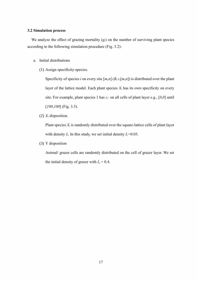
3.2 Simulation process

We analyze the effect of grazing mortality (gi) on the number of surviving plant species

according to the following simulation procedure (Fig. 3.2):

a. Initial distributions

(1) Assign specificity-species.

Specificity of species i on every site [m,n] (Bi ɛi[m,n]) is distributed over the plant

layer of the lattice model. Each plant species Xi has its own specificity on every

site. For example, plant species 1 has ɛ1 on all cells of plant layer e.g., [0,0] until

[100,100] (Fig. 3.3).

(2) Xi disposition.

Plant species Xi is randomly distributed over the square-lattice cells of plant layer

with density Ii. In this study, we set initial density Ii =0.03.

(3) Y disposition

Animal/ grazer cells are randomly distributed on the cell of grazer layer. We set

the initial density of grazer with Iy = 0.4.

18

Figure 3.2 Simulation process of lattice model. (a) Simulation flowchart of the model.

(b) Main processes of the lattice model.

a

b

19

Figure 3.3 Specificity species i on every lattice site [m,n]

b. Reproduction process

The reproduction process is run in plant layer. The process is proceeded with

following procedure;

(1) To choose a cell of plant layer.

First, a cell on plant layer is chosen randomly (Figs. 3.4a).

(2) To choose a neighbor of the chosen cell.

If there is plant Xi on that cell then one more cell is chosen randomly within the

dispersal range of the chosen plant species Xi (Figs. 3.4b, c).

(3) Chosen neighbor cell is change to Xi.

If the second chosen cell is vacant then plant species Xi occupies the vacant cell

with the rate of bi (Fig. 3.4d).

20

(4) First chosen cell occupied/unoccupied.

However, if the first chosen cell is vacant then the reproduction process is

ended and the process moves to grazing process, while the chosen cell remains

unchanged.

(5) Chosen neighbor cell occupied/unoccupied, bi is higher/lower than temporal

boundary.

Also, if the second chosen cell is occupied by a plant species Xi. and/ or bi is

lower than the temporal boundary then the reproduction process is ended and

the process moves to grazing process, while the second chosen cell remains

unchanged.

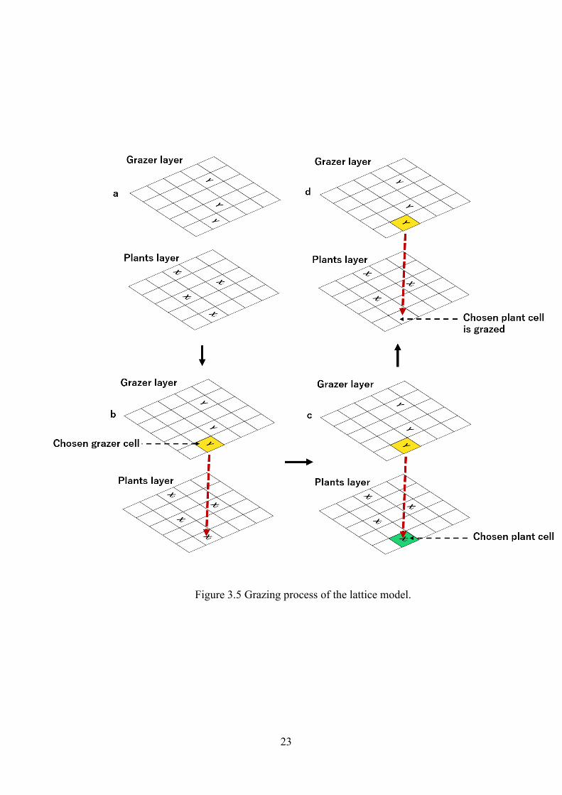
c. Grazing process

Grazing process involve both grazer layer and plant layer. The process is proceeded

with the following procedure;

(1) To choose a cell of grazer layer.

First, we choose a cell randomly on the grazer layer (Figs. 3.5a, b).

(2) To choose a plant cell.

If there is a grazer or an animal Y on that cell then one cell with the same position

[m,n] with the chosen grazer cell on the plant layer is selected (Fig. 3.5b).

(3) Plant cell changed to vacant.

If there is a plant species Xi. on the plant layer and the rate gi is higher to temporal

boundary then that cell is grazed by grazer Y with (Fig. 3.5 d).

(4) Chosen grazer cell is unoccupied.

However, if there is no grazer/animal on the chosen cell of animal layer then the

process is ended, and the cell remains unchanged. The process moves to check

number of grazing time (k).

21

(5) Chosen plant cell unoccupied

Also, if there is no plant species Xi on the plant layer then the process is ended

and the cell remains unchanged. The process moves to check the number of

grazing time (k).

(6) To check the k grazing times.

If the number of grazing times is satisfied e.g., k = 3, then the process moves to

the next step. But if number of grazing time (k) is not satisfied, then grazing

process is repeated from the beginning.

d. Repetition process

(1) Reproduction and grazing process are repeated LL and kLL times,

respectively. refers to the number of square-lattice cell and k denotes the

grazing time.

(2) 1 step in the simulation means 1-time reproduction process and k time grazing

process. In addition, LL and kLL times refer to 1 run which is repeated from

grazer Y distribution process.

(3) Processes in a is repeated for 30 trials. 1 trial means the process is repeated from

assigning specificity species on lattice sites for 10,000 runs (Fig. 3.2).

LL

22

Figure 3.4 Reproduction process of the lattice model

23

Figure 3.5 Grazing process of the lattice model.

24

3.2 Research tools

We mainly used two computer machines to run the simulations. The computer’s

specification is as the following:

a. Computer machine 1

• Processor Intel(R) Core(TM) i7-4790K CPU @4.00 GHz 4.00 GHz.

• RAM memory is 16 GB.

• Operating system (OS) is Windows 10 Pro.

• System type is 64-bit operating system, x64 based processor

b. Computer machine 2

• Processor Intel(R) Core(TM) i7-4790K CPU @4.00 GHz 4.00 GHz

• RAM memory is 16 GB (15.7GB usable).

• Operating system (OS) is Windows 10 Home.

• System type is 64-bit operating system, x64 based processor.

25

4. Results

4.1 The effect of species-independent factors

In an early stage of the present study, we only considered the opposite case for grazing

mortality. We studied the effect of grazing period k and grazing intensity G on the number of

surviving species (Figs. 4.1b, d). The number of surviving plant species responds unimodally

on the grazing intensity G (Fig. 4.1b). The increase of grazing times maintains the unimodal

behavior with the decrease of number of survivors. We investigated the effect of k grazing

time and fecundity B on the reproduction of plant species (Figs. 4.1a, c). The coexisting

species increases with the increase of fecundity B (Fig. 4.1a). The results also indicated the

importance of the interspecific grazing difference G’ to promote coexistence of plant species

(Figs. 4.1b-d).

Previous studies show that animal grazer might tend to feed on a more dominant species,

a tradeoff. We studied the effect of the tradeoff on the number of survivors (Figs. 4.2b-d).

Surprisingly, more plant species can survive (Fig. 4.2b). The number of survivors is also

higher given various values of fecundity B, compared to the opposite case (Fig. 4.2a).

Similarly, G’ is necessary for unimodality in the tradeoff case (Figs. 4.2b-d).

Proceeding the investigations, we simulated various dispersal rates and lattice sizes (Figs.

4.3a, b). The dispersal rates do not show any significant effect on the number of survivors

(Fig. 4.3a). Similarly, the number of species increase proportionally with the increase of the

lattice sizes (Fig. 4.3b). We examined the processing time of the simulation on each set

parameter values which is also a consideration to determine the repetition of simulations

(Figs. 4.4a, b). On average, high grazing maintains low density and low grazing showed a

higher species density. (Figs. 4.5a, b).

26

Figure 4.1 The number of surviving species as a function of the basal grazing intensity G or

basal fecundity B for various values of grazing times k. (a-d) The grazing intensity increases

as the initial birth rate decreases, i.e., ( )' 1ig G G i= + − and Bi = B-0.002(i-1) for i=1, 2, …,

s), indicating that inferior species are eaten more often by grazers. (a, b) The value of the

species-dependent factor is G' = 0.0005. (c, d) The value of the species-dependent factor is

G' = 0. (b) Fecundity B = 1. The lattice size is 100 x100. The dispersal rate is P = 40. The

initial species density is Ii = 0.03 (same for all species). The density of grazer cells is Iy = 0.4.

Error bars indicate the standard deviations.

Nu

mb

er

of

su

rviv

ing

pla

nt

sp

ec

ies

Grazing intensity GBasal fecundity B

a b

c d

27

Figure 4.2 The number of surviving species as a function of the basal grazing intensity G or

basal fecundity B for various values of grazing times k. (a-d) The grazing rate of a species

increases as the fecundity increases, i.e., ( )' 20ig G G i= + − and Bi = B-0.002(i-1) for i=1,

2, …, s), indicating a tradeoff between the birth rate and grazing intensity of a species. (a, b)

The value of the species-dependent factor is G' = 0.0005. (c, d) The value of the species-

dependent factor is G' = 0. (b) Fecundity B = 1. The lattice size is 100 x100. The dispersal

rate is P = 40. The initial species density is Ii = 0.03 (same for all species). The density of

grazer cells is Iy = 0.4. Error bars indicate the standard deviations.

Nu

mb

er

of

su

rviv

ing

pla

nt

sp

ec

ies

Grazing intensity GBasal fecundity B

a b

c d

28

Figure 4.3. The effects of dispersal range and lattice size on the number of surviving species

in a grassland community under grazing. (a-d) The grazing rate of a species increases as the

fecundity increases, i.e., ( )' 20ig G G i= + − and Bi = B-0.002(i-1) for i=1, 2, …, s),

indicating a tradeoff between the birth rate and grazing intensity of a species. The birth rate

is Bi = B-0.002(i-1), where B = 1. (a-d) G’ = 0.0005, G = 0.15. The lattice size is 100 x100

for (a). The dispersal rate is P = 40 for (b). The initial species density is Ii = 0.03 (same for

all species). The density of grazer cells is Iy = 0.4. Error bars indicate the standard deviations.

a

Nu

mb

er

of

su

rviv

ing

sp

ec

ies

Dispersal rate Lattice size

b

29

b

a

Grazing intensity G

Nu

mb

er

of

su

rviv

ing

pla

nt

sp

ec

ies

Fecundity B

30

Figure 4.4 The processing time of the number of surviving species as a function of the basal

grazing intensity G or basal fecundity B for various values of grazing times k. The label of

each point shows the processing time (in hours) from the beginning of simulation e.g. G = 0.

(a, b) The grazing rate of a species increases as the fecundity increases, i.e.,

( )' 20ig G G i= + − and Bi = B-0.002(i-1) for i=1, 2, …, s), indicating a tradeoff between

the birth rate and grazing intensity of a species. (a, b) The value of the species-dependent

factor is G' = 0.0005. (a, b) The value of the species-dependent factor is G' = 0.0005. (b)

Fecundity B = 1. The lattice size is 100 x100. The dispersal rate is P = 40. The initial species

density is Ii = 0.03 (same for all species). The density of grazer cells is Iy = 0.4. Error bars

indicate the standard deviations.

31

Figure 4.5 Temporal dynamic of surviving plant species density. (a, b) The grazing intensity

increases as the initial birth rate decreases, i.e., ( )' 1ig G G i= + − and Bi = B-0.002(i-1) for

i=1, 2, …, s), indicating that inferior species are eaten more often by grazers. (a, b) The value

of the species-dependent factor is G' = 0.0005. (a) The value of the species-dependent factor

is G = 0.05. (b) The value of the species-dependent factor is G = 0.5 (b) Fecundity B = 1.

The lattice size is 100 x100. The dispersal rate is P = 40. The initial species density is Ii =

0.03 (same for all species). The density of grazer cells is Iy = 0.4. Error bars indicate the

standard deviations.

Time steps

Su

rviv

ing

pla

nt

sp

ec

ies

den

sit

y

a b

32

4.2 The effect of species-dependent factors

We simulate a lattice grassland model with 20 plant species under various levels of grazing

intensity (G) without nongrazing natural mortality, i.e., di = 0 (Figs. 4.6, 4.7, 4.8, 4.13). The

temporal dynamics exhibit large fluctuations in the number of individuals of each species

over a long period of time (Figs. 4.6a, 4.7a, and 4.8a). In contrast, this number is fairly stable

over a short timescale (Figs. 4.6b, 4.7b, and 4.8b). Based on the short-term temporal

dynamics (Figs. 4.6b, 4.7b and 4.8b) and snapshots of the plant distributions (Figs. 4.6c, 4.7c

and 4.8c), the number of surviving plant species is highest at an intermediate grazing

intensity (G). At the low grazing intensity, the number of survivors is higher than high grazing

intensity (Figs. 4.6c, 4.8c).

To test the effect of grazing on species coexistence, we vary the basal grazing intensity G

to examine the effects of grazing (Figs. 4.9, 4.18, 4.19, 4.20, Table 4.1). The number of

species is highest at an intermediate grazing intensity (G) for a given fecundity B and

interspecific grazing difference G' (Fig. 4.9, 4.17b, c, e, f). The interspecific grazing

difference G' is the difference in animal preference or selectiveness in grazing, e.g., palatable

herbs or unpalatable grass. For example, grass species is more preferred than herbs for animal

grazers. To examine the effects of a tradeoff between birth rate and grazing intensity, we

consider the following opposite relations between the species-specific expected birth rate Bi

and grazing rate gi: (1) the tradeoff case: species with a high Bi have a high gi (grazing is

subject to a tradeoff) and (2) the opposite case: species with a high Bi have a low gi. In both

cases, the number of surviving species exhibits unimodal behavior in response to the grazing

intensity G. The number of coexisting species at peak diversity is larger under the first case

(with the tradeoff) than under the second case (the opposite) (Fig. 4.9).

33

If there is no interspecific grazing difference (G' = 0), then the number of surviving species

decreases monotonically with an increase in the grazing intensity G (Figs. 4.17a, d, 4.18a,

4.19a, c, e, 4.20a). However, if a slight difference (e.g., G' = 0.0005) is introduced, then the

number of species responds unimodally (Figs. 4.9, 4.17b, c, e, f, 4.18b, 4.19b, f, 4.20b).

Interestingly, the peak height (the number of surviving species) decreases as the interspecific

grazing difference G' is further increased (differences in colored lines in Figs. 4.9, 4.18b, c).

The number of coexisting species decreases as the density of grazer cells Iy increases (Figs.

4.10a-c, 4.19a, c, e). However, the unimodal behavior is preserved as long as the density of

grazer cells is kept constant (Figs. 410d-f, 4.19b, d, f, 4.20b). Natural mortality di (i.e., di =

0.1) also suppresses the unimodal behavior (Fig. 4.10f).

To understand the effect of grazing on population density, we examine the composition of

surviving species (Figs. 4.11, 4.12). In the first (tradeoff) case, the species with the lowest

grazing rate dominates at a low grazing intensity (Fig. 4.6c), and that with the highest birth

rate dominates at a high grazing intensity (Fig. 4.8c), while various species survive at low

densities at an intermediate grazing intensity (Fig. 4.7c). In contrast to the second case

(opposite to the tradeoff case) (Figs. 4.13, 4.14), however, the results of the first case (with

the tradeoff) reveal a large fluctuation when the grazing intensity G is high (Figs. 4.11, 4.12).

Here, which species survive depends on the simulation run (Figs. 4. 11c, d, 4.12 c, d). In any

case, the results converge, and monotonic behavior is recovered as G' decreases to zero (Figs.

4.17 a, d). Accordingly, the results indicate that the species dependence of grazing G' is

important for unimodality but the tradeoff between the birth rate and grazing intensity is not

essential.

34

Figure 4.6 The temporal dynamics of species density and a snapshot of the final density

composition at low grazing rate G= 0.05. (a-c) The grazing intensity of a species decreases

as the initial birth rate decreases, i.e., ( )' 20ig G G i= + − and Bi = B-0.002(i-1) for i=1,

2, …, s), indicating a tradeoff between the birth rate and grazing intensity of a species. (a)

Temporal dynamics for 10000 steps. (b) Temporal dynamics of the last one hundred steps.

(c) A snapshot of the final surviving species composition. The value of the species-dependent

factor is G' = 0.0005. The lattice size is 100 x100. The dispersal rate is P = 40. The initial

species density is Ii = 0.03 (same for all species). The density of grazer cells is Iy = 0.4. Error

bars indicate the standard deviations.

a b

c

Plan

t spe

cies

den

sity

Spec

ies

i

Time step

35


composition at intermediate grazing rate G= 0.15. (a-c) The grazing intensity of a species

decreases as the initial birth rate decreases, i.e., ( )' 20ig G G i= + − and Bi = B-0.002(i-1)

for i=1, 2, …, s), indicating a tradeoff between the birth rate and grazing intensity of a species.

a) Temporal dynamics for 10000 steps. (b) Temporal dynamics of the last one hundred steps.





a b

c

Plan

t spe

cies

den

sity

Spec

ies

i

Time step

36


composition at high grazing rate G= 0.4. (a-c) The grazing intensity of a species decreases

as the initial birth rate decreases, i.e., ( )' 20ig G G i= + − and Bi = B-0.002(i-1) for i=1,

2, …, s), indicating a tradeoff between the birth rate and grazing intensity of a species. (a)

Temporal dynamics for 10000 steps. (b) Temporal dynamics of the last one hundred steps.





a b

c

Plan

t spe

cies

den

sity

Spec

ies

i

Time step

37

Nu

mb

er

of

su

rviv

ing

pla

nt

sp

ec

ies

Grazing intensity G

B =

1B

= 0

.75

B =

0.5

a

b

c

d

e

f

38

Figure 4.9 The number of surviving species as a function of the basal grazing intensity G for

various values of interspecific grazing differences (G'). Three different values of the basal

birth rate are shown: (a, d) B= 1; (b, e) B= 0.75; and (c, f) B= 0.5. (a-c) The grazing intensity

of a species decreases as the initial birth rate decreases, i.e., ( )' 20ig G G i= + − and Bi = B-

0.002(i-1) for i=1, 2, …, s), indicating a tradeoff between the birth rate and grazing intensity

of a species. (d-f) The grazing intensity increases as the initial birth rate decreases, i.e.,

( )' 1ig G G i= + − and Bi = B-0.002(i-1) for i=1, 2, …, s), indicating that inferior species are

eaten more often by grazers. The value of the species-dependent factor is G' = 0.0005. The

lattice size is 100 x100. The dispersal rate is P = 40. The initial species density is Ii = 0.03

(same for all species). The density of grazer cells is Iy = 0.4. Error bars indicate the standard

deviations.

39

Nu

mb

er

of

su

rviv

ing

pla

nt

sp

ec

ies

Grazer cell Iy

a

b

c

Grazing intensity G

d

e

f

d=0.001

d=0.01

d=0.1 d=0.1

d=0.01

d=0.001

40

Figure 4.10 The effects of the animal density Iy on the number of surviving species under

various basal grazing intensities (G) and natural mortalities (di). (a-c) The grazing intensity

of a species decreases as the fecundity decreases, i.e., ( )' 20ig G G i= + − and Bi = B-

0.002(i-1) for i=1, 2, …, s), indicating a tradeoff between the birth rate and grazing intensity

of a species. (a-c) G’ = 0.0005. The lattice size is 100 x100. (a-c) The grazing intensity is

0.15. The dispersal rate is P = 40. The initial species density is Ii = 0.03 (same for all species).

(d-f) The density of grazer cells is Iy = 0.4. Error bars indicate the standard deviations.

41

Figure 4.11 Population densities of species with respect to the basal grazing intensity G for

the tradeoff case. (a-d) The grazing intensity of a species increases as the fecundity increases,

i.e., ( )' 20ig G G i= + − and Bi = B-0.002(i-1) for i=1, 2, …, s), indicating a tradeoff

between the birth rate and grazing intensity of a species. (a-d) The result of a single run. (e-

h) The average of 30 runs. The basal grazing rates are (a) G= 0.05, (b) G= 0.1, (c) G = 0.3,

and (d) G = 0.5. The parameters are as follows: interspecific grazing difference, G’ = 0.0005;

basal fecundity, B= 1; initial species density, Ii = 0.03 (for all species); density of grazer cells,

Iy = 0.4; and dispersal rate, P = 40. The lattice size is 100 x100.

a b

c d

Po

pu

lati

on

of

pla

nt

sp

ec

ies

de

ns

ity

Species i

42


the tradeoff case. (a-d) The grazing intensity of a species increases as the fecundity increases,


between the birth rate and grazing intensity of a species. (a-d) The average result of 30 runs.

The basal grazing rates are (a) G= 0.05, (b) G= 0.1, (c) G = 0.3, and (d) G = 0.5. The

parameters are as follows: interspecific grazing difference, G’ = 0.0005; basal fecundity, B=

1; initial species density, Ii = 0.03 (for all species); density of grazer cells, Iy = 0.4; and

dispersal rate, P = 40. The lattice size is 100 x100.

a b

c d

Species i

Po

pu

lati

on

of

pla

nt

sp

ecie

s d

en

sit

y

43


the opposite case. (a-d) The grazing intensity decreases as the fecundity increases, i.e.,


eaten more often by grazers. (a-d) The result of a single run. The basal grazing rates are (a)

G= 0.05, (b) G= 0.1, (c) G = 0.3, and (d) G = 0.5. The parameters are as follows: interspecific

grazing difference, G’ = 0.0005; basal fecundity, B= 1; initial species density, Ii = 0.03 (for

all species); density of grazer cells, Iy = 0.4; and dispersal rate, P = 40. The lattice size is 100

x100.

a b

c d

Po

pu

lati

on

of

pla

nt

sp

ec

ies

de

ns

ity

Species i

44


the opposite case. (a-d) The grazing intensity decreases as the fecundity increases, i.e.,


eaten more often by grazers. (a-d) The average result of 30 runs. The basal grazing rates are

(a) G= 0.05, (b) G= 0.1, (c) G = 0.3, and (d) G = 0.5. The parameters are as follows:

interspecific grazing difference, G’ = 0.0005; basal fecundity, B= 1; initial species density, Ii

= 0.03 (for all species); density of grazer cells, Iy = 0.4; and dispersal rate, P = 40. The lattice

size is 100 x100.

a b

c d

Species i

Po

pu

lati

on

of

pla

nt

sp

ec

ies

de

ns

ity

45

Figure 4.15 The average number of surviving species as a function of the basal grazing

intensity G and basal fecundity B for three values of interspecific grazing differences (G').

(a-c) The grazing intensity of a species increases as the fecundity increases, i.e.,

( )' 20ig G G i= + − and Bi = B-0.002(i-1) for i=1, 2, …, s), indicating a tradeoff between the

birth rate and grazing intensity of a species. The values of interspecific grazing differences

are (a) G’= 0.0005, (b) G’= 0.001, and (c) G’= 0.0015. The lattice size is 100 x100. The

dispersal rate is P= 40. The initial species density is Ii = 0.03 (same for all species). The

density of grazer cells is Iy = 0.4.

a

Pla

nt

sp

ec

ies

fe

cu

nd

ity

B

b c

Grazing intensity G

46

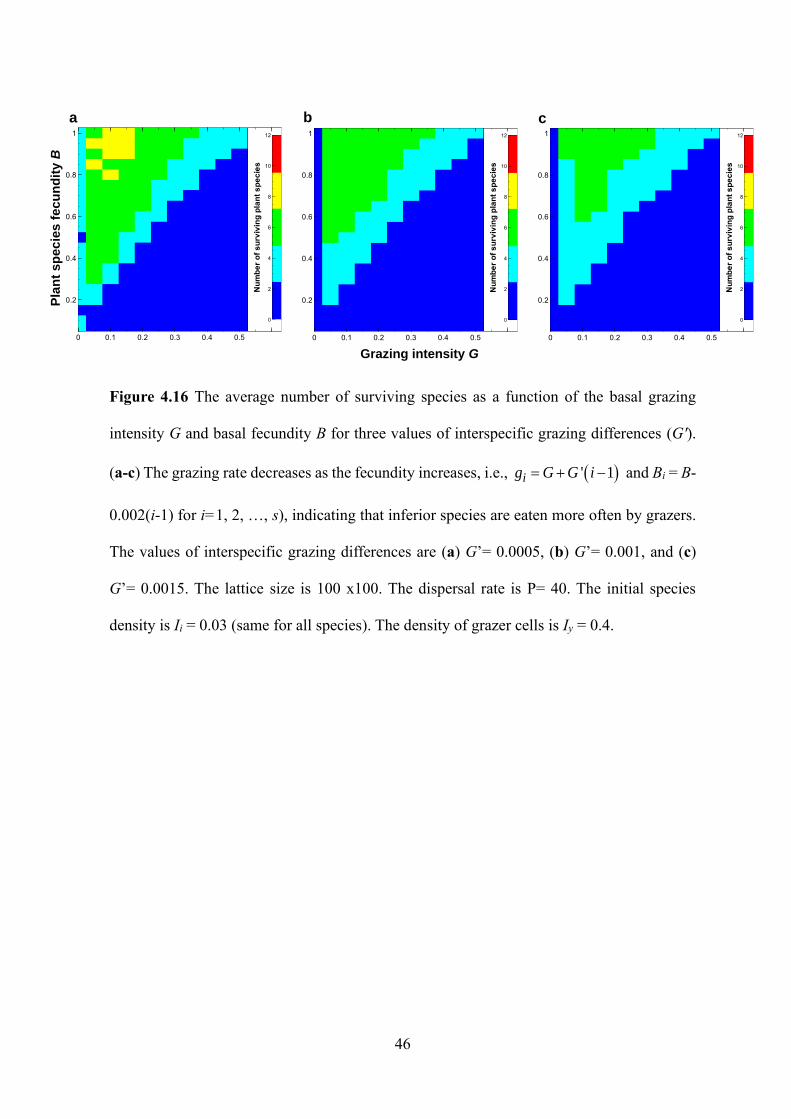
Figure 4.16 The average number of surviving species as a function of the basal grazing

intensity G and basal fecundity B for three values of interspecific grazing differences (G').

(a-c) The grazing rate decreases as the fecundity increases, i.e., ( )' 1ig G G i= + − and Bi = B-

0.002(i-1) for i=1, 2, …, s), indicating that inferior species are eaten more often by grazers.

The values of interspecific grazing differences are (a) G’= 0.0005, (b) G’= 0.001, and (c)

G’= 0.0015. The lattice size is 100 x100. The dispersal rate is P= 40. The initial species

density is Ii = 0.03 (same for all species). The density of grazer cells is Iy = 0.4.

a b

Grazing intensity G

c

Pla

nt

sp

ec

ies

fe

cu

nd

ity

B

47

a

b

Nu

mb

er

of

su

rviv

ing

pla

nt

sp

ec

ies

Grazing intensity G

c

d

e

f

48

Figure 4.17 The number of surviving species as a function of the basal grazing intensity G

for various values of the basal birth rate B with G' = 0. (a-c) The grazing intensity of a species


2, …, s), indicating a tradeoff between the birth rate and grazing intensity of a species. (d-f)

The grazing intensity decreases as the fecundity increases, i.e., ( )' 1ig G G i= + − and Bi = B-

0.002(i-1) for i=1, 2, …, s), indicating that inferior species are eaten more often by grazers.

The differences in the interspecific grazing rate are (a, d) G’= 0, (b, d) G’= 0.0005, and (c,

f) G’= 0.0015. The lattice size is 100 x100. The dispersal rate is P = 40. The initial species

density is Ii = 0.03 (same for all species). The density of grazer cells is Iy = 0.4. Error bars


49

ba

c

a

Grazing intensity G

Grazing intensity G

50

Figure 4.18 The effect of the interspecific grazing difference value G' on the number of

surviving species. (a-c) The grazing intensity of a species increases as the fecundity increases,


between the birth rate and grazing intensity of a species. (a-c) G = 0.15. The lattice size is

100 x100. The dispersal rate is P = 40. The initial species density is Ii = 0.03 (same for all

species). The density of grazer cells is Iy = 0.4. Error bars indicate the standard deviations.

51

b

Grazing intensity G

Nu

mb

er

of

su

rviv

ing

pla

nt

sp

ec

ies

Animal density Iy

a

G’ =

0.0

01

G’ =

0G

’ =

0.0

005

dc

fe

52

Figure 4.19 The effect of the animal density Iy, basal grazing rate G, and interspecific grazing

difference G' on the number of surviving species. (a-f) The grazing intensity of a species


2, …, s), indicating a tradeoff between the birth rate and grazing intensity of a species. The

differences in the interspecific grazing rate are (a-b) G’ = 0 (c-d) G’ = 0.0005 (e-f) G’ =

0.001. The lattice size is 100 x100. The dispersal rate is P = 40. The initial species density is

Ii = 0.03 (same for all species). Error bars indicate the standard deviations.

53

Figure 4.20 The effect of the animal density Iy, basal grazing rate G, and interspecific grazing

difference G' on the number of surviving species. (a-b) The grazing intensity of a species


2, …, s), indicating a tradeoff between the birth rate and grazing intensity of a species. (b)

G’ = 0.0005. The lattice size is 100 x100. The dispersal rate is P = 40. The initial species

density is Ii = 0.03 (same for all species). (a) The density of grazer cells is Iy = 0.4. Error bars


b

Animal density Iy

Gra

zing

inte

nsity

Ga

Interspecific grazing difference G’

54

Table 4.1 Number of surviving species based on the grazing intensity G and interspecific

grazing difference G'. The grazing intensity of a species increases as the fecundity increases,


between the birth rate and grazing intensity of a species. The lattice size is 100 x100. The

dispersal rate is P= 40. The initial species density is Ii = 0.03 (same for all species). The

density of grazer cells is Iy = 0.4.

G’ G

0 0.05 0.1 0.15 0.2 0.25 0.3 0.35 0.4 0.45 0.5

0.00001 20.00 14.57 11.03 9.63 8.37 7.23 6.13 5.10 4.67 3.77 3.07

0.00002 20.00 14.07 11.37 9.50 8.60 7.37 6.50 5.20 4.17 3.90 2.93

0.00003 19.93 14.50 11.43 9.70 8.60 7.17 6.57 5.40 4.50 3.77 3.07

0.00004 18.40 15.40 11.20 9.77 8.50 7.40 6.30 5.33 4.57 3.67 3.00

0.00005 15.50 15.47 11.83 9.87 8.50 7.40 6.40 5.30 4.80 3.73 3.03

0.00006 13.20 16.10 12.20 9.87 8.40 7.57 6.40 5.57 4.47 3.60 3.07

0.00007 12.00 16.43 12.03 10.17 8.63 7.10 6.23 5.67 4.67 3.60 3.20

0.00008 10.20 16.70 12.50 10.13 8.63 7.60 6.50 5.57 4.27 3.70 3.07

0.00009 9.37 16.47 12.70 10.40 8.47 7.73 6.50 5.20 4.57 3.70 2.90

0.0001 8.73 17.03 12.43 10.33 8.73 7.50 6.03 5.40 4.67 3.77 2.93

0.0002 5.00 14.50 13.60 10.93 8.87 7.63 6.57 5.10 4.57 3.80 2.97

0.0003 3.80 11.33 13.50 11.70 9.33 7.70 6.53 5.33 4.50 3.70 3.13

0.0004 3.07 9.43 11.70 11.40 10.13 8.07 6.50 5.77 4.57 3.57 2.83

0.0005 2.53 8.37 10.40 11.17 9.67 7.83 6.87 5.43 4.47 4.07 2.80

0.0006 2.57 7.70 9.47 10.13 9.73 8.37 6.80 5.57 4.63 3.67 2.87

0.0007 2.47 7.17 8.50 9.50 9.30 8.27 6.77 5.67 4.43 3.63 2.97

0.0008 2.37 7.10 8.23 9.13 8.93 8.07 6.87 5.80 4.50 3.63 2.73

0.0009 2.17 6.53 7.67 8.47 8.30 8.03 6.87 5.67 4.73 3.63 2.73

55

5. Discussion

In the present thesis, it is shown that our model simulation is able to reproduce the

empirical observation of species diversity maintained by grazing animals. This thesis

presents the first possible mechanism to explain the enhancement of species diversity by

grazing. Our result confirms that the coexistence of plant species is possible under grazing

in grasslands (Figs. 4.6, 4.7, 4.8). The results reveal unimodality in which the peak species

diversity occurs at an intermediate grazing intensity (Fig. 4.9). When there is a tradeoff

between the birth rate and grazing rate, the number of coexisting species is large (more than

10 species) (Figs. 4.9a-c). Therefore, this tradeoff promotes coexistence by balancing

competitiveness among all plant species. We also test the case in which the grazing rate is

negatively correlated with the birth rate. Surprisingly, unimodality in response to grazing

intensity is still observed (Figs. 4.9d-f). In this case, the intermediate grazing rate allows less

superior species to persist by occupying the new vacant sites produced by grazers (Figs.

4.13b, 4.14b), while it is not strong enough to exclude them (as in Figs. 4.13d, 4.14d). Thus,

the coexistence of species is mechanically promoted because (weak) grazing produces vacant

sites available for other species. The number and composition of coexisting species vary

depending on simulation runs (Figs. 4.11a-d, 4.13a-d), while on average they are determined

by the birth rate and grazing mortality rate (Figs. 4.12a-d, 4.14a-d). The tradeoff between the

birth rate and grazing rate is not necessary for the unimodality in response to grazing intensity.

According to the presented results, species coexistence ceases to be maintained if natural

mortality caused by other factors is introduced (Figs. 4.10d-f, 4.17a, d, and 4.18). Therefore,

an increase in diversity due to grazing does not occur when grazing is not the principal source

of mortality in grasslands, i.e., when the nongrazing mortality is not negligible. This

56

prediction should be tested empirically in future field studies. The interspecific grazing

difference G' also plays an important role in the promotion of coexistence. If the difference

is absent or very minute, then the promotion of coexistence by grazing disappears (Fig. 4.18a

vs Figs. 4.18b, 4.18c).

It should be remarked that the composition of surviving species depends on how the birth

rate varies compared to the variation of grazing mortality (Figs. 4.11, 4.12, 4.13, 4.14). In

the tradeoff case, inferior species (with low birth rates) exclude superior species (with high

birth rates) (Figs. 4.9a-c). In the opposite case, superior species dominate the grassland (Figs.

4.9d-f). The composition of surviving species is highly variable in the tradeoff case but stable

in the opposite case (Figs. 4.11, 4.12, 4.13, 4.14). These results should be verified empirically

in managed grasslands. Furthermore, the current simplified assumptions about grazing rate

gi may be modified explicitly to include the behavior of grazing animals, e.g., the frequency

dependence in food-plant selection.

The effects of herbivores on plant diversity in grasslands have been analyzed by using

empirical data [65, 66, 67]. The proposed grazing model integrated with a microhabitat

locality model [36] should be sufficient as a canonical model with which to investigate the

functional mechanisms of herbivore grazing effects mathematically. In terms of maintaining

and increasing diversity, our results are in line with those of some empirical studies [14, 38-

42, 68-73]. For example, Komac et al. stated that maintaining an adequate grazing intensity

(avoiding both abandonment and overgrazing) is necessary to preserve diversity in grasslands

[38]. Mu et al. also found that light and moderate grazing promote plant biodiversity [39]. In

addition, Chen et al. showed that heavy grazing has an indirect influence on biodiversity [42].

Furthermore, Chen et al. based on empirical observation inferred that grazing type and

57

vegetation structure that affect spatial variation are the reasons for the high species richness

in the Qinghai alpine meadow [14]. The two reasons are in line with our models and results.

In a grassland where grazing is not the only main mortality factors, intermediate grazing

intensity is also necessary to maintain diversity. Joubert et al. found that coupling fire

disturbance and moderate grazing can maintain plant diversity [41]. They measured the

species richness was significantly higher at recently burned grassland and coupled with

moderate grazing intensity. Their results conform to our model (Figure 4.10) that in grassland

where nongrazing mortality is not negligible, the unimodality is still maintained when

nongrazing mortality is kept at a low rate or in nature grazing has sufficient time to increase

diversity after the burning. Collin et al. also revealed that grazing even reverses the loss of

diversity caused by frequent burning [68]. They also showed that in two long-term field

experiments, diversity decreased on burned and fertilized treatments, while grazing

preserved diversity under the same conditions. The studies imply that grazing naturally

maintains plant diversity in various conditions.

The studies on herbivore in grasslands are in line with our result that, for example, trade-

off cases where animal grazers prefer dominant plant species, resulting in higher plant

diversity [65, 66, 73]. Animal grazer Assemblages, including large herbivores, animals with

weight > 30kg increased plant diversity at higher productivity of grassland areas [65].

Usually, large animals tend to feed on dominant plant species. The preferred grasses

decreased significantly under heavy grazing (large animal grazer) but increased without

grazing [73]. However, when light (a small number of grazers) and moderate (moderate

number of grazers) grazing is introduced, the proportion of less dominant species increased.

58

As for an example of the field experiment, Hasbagan et al. measured the species diversity

in under four grazing levels [no grazing, light(2.4 sheep units ha–1), moderate (3.6 sheep

units ha–1), and heavy (6.0 sheep units ha–1) grazing] in 5 years (2006–2010) grassland in

Qinghai-Tibetan Plateau. They measured the number of species to determine the species

richness on the plot objects. They found that moderate grazing enhanced the species diversity

higher than light and heavy, and twice higher than without grazing [73]. This study is in line

with our result that the number of less superior species increases under moderate grazing

intensity, whereas preferred species tend to decrease, depends on grazing intensity or

assemblage of animal grazer in nature [65, 66, 67]. Studies by McNaughton, known for his

work in Serengeti, also found that the moderate grazing stimulated productivity up to twice

higher than in ungrazed plots [17]. Animal grazing increases the overall productivity of

grassland by invoking the recovery action in grass species more than that without grazing

[18]. The grazing increases the productivity of plant species even after the loss by grazing.

In principle, the numerical values of the parameters may be evaluated from empirical data

of the birth and death rates of coexisting plant species. However, in practice, it has yet to be

done because each grassland ecosystem is uniquely complex in a substantial manner. In a

grassland community consisting of more than ten species, the birth and death rates of each

species is almost impossible to trace over time. The only available data are the number of

species (species diversity) and the covers of each species at time in a community [14, 37].

One possible approach to test the current simulation results is the use of an experimental

pasture where the number of grass species are limited to 10 to 20 species [54]., but

surrounded by natural grasslands with many more species. We divide the experimental plot

into several plots with different density of grazing. In this approach, we may be able to test

directly the effects of animal grazing on plant species diversity. We may be able to test if low

59

level of grazing will increase the number of plant species. Note here the new species should

have invaded from the surrounding natural grasslands. Recently a similar approach has been

taken to show that grazing enhances species richness [74]. However, the direct empirical

demonstration of the current simulation results is still very difficult. Thus, the empirical proof

of this model is a future problem of grassland ecosystems.

Moreover, by modifying the lattice setting, the current model can be applied to other

terrestrial communities while considering predators. However, this mechanism of grazer or

predator effects should be directly verified using empirical data in the future.

We should also note that this grazing model presents similar results with the intermediate

disturbance models [34, 43, 44, 75,76]. In these models, there may be several specific

underlying mechanisms promoting coexistence. Intermediate disturbance hypotheses stated

that disturbances such as fire, flood, and even deforestation by humans might promote

diversity if they occur at the intermediate level. Qualitatively the current grazing model

appears to conform to these models. Because our model also achieves the highest diversity

at the intermediate level of grazing. However, whether the current model is considered as

one such specific mechanism or not is a future issue.

60

6. Conclusion

The study presented in this dissertation is a significant contribution to elucidate the actual

grazing behavior of grasslands in the area of ecological fields. Scientists had performed many

empirical studies to test the effect grazing for decades. However, no convincing explanation

was provided for the unimodal response of grazing. We believe that it would take decades or

even hundreds of years to verify the grazing mechanism experimentally. Owing to the vast

area covering one-quarter of the Earth’s land area, various conditions of the environment,

and many other complicated factors changing through time, it appears almost impossible to

examine grazing effect to conclude a universal understanding of the plant species

coexistence in grasslands. Therefore, we conduct the research to verify the effect of grazing

on species coexistence using mathematical and simulation methods. Simulations studies have

been advanced with the development of technology. The recent computer technology allows

for more realistic and accurate simulations.

We used a lattice model to analyze how grazing influences the grassland’s diversity. Our

model revealed that the coexistence of multiple species is possible with the existence of

grazers. The results exhibit that intermediate grazing intensity causes the peak of unimodality,

which signifies the highest number of surviving plant species. The animal grazers produce

vacant sites in which inferior species can inhabit. Grazing also moderates the

competitiveness to feed on more palatable dominant plant species. This is shown to occur in

the tradeoff case. We also test the opposite case that the dominant species is more unpalatable

for grazers. The result still maintains coexistence with a smaller number of survivors. The

coexisting species depends on the interspecific relationship between birth rate and grazing

mortality rate. In the tradeoff case, the surviving species is inconsistent with the grazing

effect. Inferior species dominate at a low grazing rate while superior species do at a high

61

grazing rate. However, both superior and inferior species coexist at the intermediate grazing

rate. In the opposite case, superior species dominate at all grazing intensities. Introduction of

nongrazing mortality leads to elimination of the promotion of coexistence. Moreover, an

increase in diversity does not occur when grazing is not the primary mortality source. The

seed dispersal of plant species is also an important factor, while the range of dispersal does

not significantly affect the promotion of diversity.

This research provides the first possible mechanism that explains the grazing effect in

grassland species coexistence. The model can be extended to consider other parameters

capturing other essential features of grasslands. The specific dependence of species and

lattice sites can be modified to represent a more realistic grassland’s dynamics. The

assemblages of grazers are also possible to be incorporated in the model. In our model, the

grazer’s appetite properties are assigned specific values depending on plant species. A new

parameter can be defined to test the effect of grazer’s diversity on grassland’s coexistence.

The model can also include factors such as climate change and disturbances. Furthermore,

this model can be modified for other plant communities with the existence of predators.

62

References

1. Cardinale, B., Duffy, J., Gonzalez, A. et al. Biodiversity loss and its impact on

humanity. Nature 486, 59–67 (2012).

2. Joppa, L. N., Roberts, D. L., Pimm, S. L. How many species of flowering plants are

there? P. ROY. SOC. B-BIOL. SCI. 278, 1705 (2010).

3. Mora, C., Tittensor, D. P., Adl, S., Simpson, A. G. B., Worm. B. How Many Species Are

There on Earth and in the Ocean? PLoS Biol. 9 (8) (2011).

4. May, R. M. Why Worry about How Many Species and Their Loss? PLoS Biol. 9 (8)

(2011).

5. Raven, P. H. Disappearing species: A global tragedy. Futurist 19, 8-14 (1985).

6. Campbell, N.A. Biology, 4th Edition. (The Benjamin/Cummings Publishing Company,

Inc., Menlo Park, California 1996).

7. Ketchum, R.M. Secret Life of the Forest. (American Heritage Press, New York, 1970.)

8. Spurr, S.H., and B.V. Barnes. Forest Ecology. (John Wiley & Sons, New York, 1980.)

9. Prentice, L. C., Cramer, W. et al. A global biome model based on plant physiology and

dominance, soil properties and climate. J. Biogeogr. 19, 117-134 (1992).

10. Perry, D.A. Forest Ecosystems. (The Johns Hopkins University Press, Baltimore, 1994).

11. Chernov, Y.I. The Living Tundra. (Cambridge University Press, Cambridge, 1985).

12. Wilson, J. B., Peet, R. K., Dengler, J., Pärtel, M. Plant species richness: The world records.

J. Veg. Sci. 23, 796-802 (2012).

13. Loveland, T. R., et al. Development of a global land cover characteristics database and

IGBP DISCover from 1 km AVHRR data. Int. J. Remote Sens. 21, 1303-1330 (2000).

14. Chen, J., et al. Small-scale species richness and its spatial variation in an alpine meadow

on the Qinghai-Tibet Plateau, Ecol. Res. 23, 657-663 (2007).

63

15. Chytrý, M., et al. The most species-rich plant communities in the Czech Republic and

Slovakia (with new world records). Preslia 87, 217-218 (2015).

16. Plumtre. A. J., et al. Biodiversity Surveys of Murchison Falls Protected Area. Wildlife

conservation society (2015). Retrieved from Wildlife Conservation Society website:

https://uganda.wcs.org/DesktopModules/Bring2mind/DMX/Download.aspx?EntryId=3

0244&PortalId=141&DownloadMethod=attachment

17. McNaughton, S. J. Grazing as an optimization process: grass-ungulate relationships in

the Serengeti. Am. Nat. 113: 691-703 (1979).

18. McNaughton, S. J. Serengeti migratory wildebeest: facilitation of energy flow by grazing.

Science 191: 92-94. (1976).

19. Anderson, T.M., Ritchie, M.E., McNaughton, S.J. Rainfall and soils modify plant

community response to grazing in Serengeti National Park. Ecology 88 (5) 1191-1201

(2007).

20. Hector, A., et al. Plant Diversity and Productivity Experiments in European Grasslands.

Science 286, 1123-1127 (1999).

21. Tilman, D., et al. The Influence of Functional Diversity and Composition on Ecosystem

Processes. Science 277, 1300-1302 (1997).

22. Cardinale, B. J. et al. Impacts of plant diversity on biomass production increase through

time because of species complementarity. Proc. Natl. Acad. Sci. U.S.A. 104, 18123–

18128 (2007).

23. Isbell, F., Calcagno, V., Hector, A. et al. High plant diversity is needed to maintain

ecosystem services. Nature 477, 199–202 (2011).

24. O'Mara, F P. The role of grasslands in food security and climate change. Ann. Bot. 110,

1263-1270 (2012).

https://uganda.wcs.org/DesktopModules/Bring2mind/DMX/Download.aspx?EntryId=30244&PortalId=141&DownloadMethod=attachment

https://uganda.wcs.org/DesktopModules/Bring2mind/DMX/Download.aspx?EntryId=30244&PortalId=141&DownloadMethod=attachment

64

25. T. Fetzel, P. Havlik, M. Herrero, K.H. Erb. Seasonality constraints to livestock grazing

intensity. Glob. Chang. Biol. 23, 1636-1647 (2017).

26. Tilman, D., Reich, P. & Knops, J. Biodiversity and ecosystem stability in a decade-long

grassland experiment. Nature 441, 629–632 (2006).

27. Isbell, F., Craven, D., Connolly, J. et al. Biodiversity increases the resistance of ecosystem

productivity to climate extremes. Nature 526, 574–577 (2015).

28. Sala, O. E., Golluscio, R. A., Lauentroth, W. K., Soriano, A. Resource partitioning

between shrubs and grasses in the Patagonian steppe. Oecologia 81, 501-505 (1989).

29. McKane, R. B., et al. Resource-based niches provide a basis for plant species diversity

and dominance in arctic tundra. Nature 415, 68-71 (2002).

30. Collins, S. L., Uno, G. E. Seed Predation, Seed Dispersal, and Disturbance in Grasslands:

A Comment. Am. Nat. 125, 866-872 (1985).

31. Vandvik, V., Goldberg, D. E. Sources of diversity in a grassland metacommunity:

quantifying the contribution of dispersal to species richness. Am. Nat. 168, 157-167

(2006).

32. Pinto, S. M., Pearson, D. E., Maron, J. L. Seed dispersal is more limiting to native

grassland diversity than competition or seed predation. Journal of Ecology 102, 1258–

1265 (2014).

33. Tilman, D. Resource Competition and Community Structure (Princeton Univ. Press,

Princeton, New Jersey, 1982).

34. Chesson, P. Mechanisms of maintenance of species diversity. Annu. Rev. Ecol. Syst. 31,

343–366 (2000).

35. Maestre, F. T., Reynolds, J. F. Spatial heterogeneity in soil nutrient supply modulates

nutrient and biomass responses to multiple global change drivers in model grassland

communities. Glob. Change Biol. 12, 2431–2441 (2006).

65

36. Tubay, J. M., et al. Microhabitat locality allows multi-species coexistence in terrestrial

plant communities. Sci. Rep. 5, 15376 (2015).

37. Shiyomi, M. et al. Spatial heterogeneity in a grassland community: Use of power law.

Ecol. Res. 16, 487–496 (2001).

38. Komac, B., Pladevall, C., Doménech, M., Fanlo, R. Functional diversity and grazing

intensity in sub-alpine and alpine grasslands in Andorra. Appl. Veg. Sci. 18, 75-85 (2015).

39. Mu, J., Zeng, Y., Wu, Q., Niklas, K. J., Niu, K. Traditional grazing regimes promote

biodiversity and increase nectar production in Tibetan alpine meadows. Agr. Ecosyst.

Environ. 233, 336-342 (2016).

40. Niu, K., He, J., Zhang, S., Lechowicz, M. J. Tradeoffs between forage quality and soil

fertility: Lessons from Himalayan rangelands. Agr. Ecosyst. Environ. 234, 31-39 (2016).

41. Joubert, L., Pryke, J. S., and Samways, M. J. Moderate grazing sustains plant diversity

in Afromontane grassland. Appl. Veg. Sci. 20, 340-351 (2017).

42. Chen, J., Shiyomi, M., Wuyunna, Hori, Y., Yamamura, Y. Vegetation and its spatial

pattern analysis on salinized grasslands in the semiarid Inner Mongolia steppe. Grassl.

Sci. 61, 121-130 (2014).

43. Chesson, P. L., Warner, R. R. Environmental Variability Promotes Coexistence in Lottery

Competitive Systems. Am. Nat. 117, 923–943 (1981).

44. Snyder, R. E., Chesson, P. Local dispersal can facilitate coexistence in the presence of

permanent spatial heterogeneity. Ecol. Lett. 6, 301–309 (2003)

45. Takenaka, A. Dynamics of seedling populations and tree species coexistence in a forest:

a simulation study. Ecol. Res. 21, 356-363 (2006).

46. Muko, S., Iwasa, Y. Species coexistence by permanent spatial heterogeneity in a lottery

model. Theor. Popul. Biol. 57, 273‐284 (2000).

66

47. Tainaka, K. Lattice model for the Lotka-Volterra system. J. Phys. Soc. Jpn. 57, 2588–

2590 (1988).

48. Tainaka, K. Stationary pattern of vortices or strings in biological systems: lattice version

of the Lotka-Volterra model. Phys. Rev. Lett. 63, 2688–2691 (1989).

49. Tainaka, K. & Fukazawa, S. Spatial pattern in a chemical reaction system: prey and

predator in the position-fixed limit. J. Phys. Soc. Jpn. 61, 1891–1894 (1992).

50. Tainaka, K. & Itoh, Y. Topological phase transition in biological ecosystems. Europhys.

Lett. 15, 399–404 (1991).

51. Kakishima, S., et al. The contribution of seed dispersers to tree species diversity in

tropical rainforests. R. Soc. Open Sci. 2, 150330 (2015).

52. Tilman, D. Dynamics and Structure of Plant Communities (Princeton Univ. Press,

Princeton, 1988).

53. Grover, J. P. Resource Competition (Springer, New York, 1997).

54. Harper, J. L. Population Biology of Plants (Academic Press, London, 1977).

55. Hardin, G. The competitive exclusion principle. Science 131, 1292-1297 (1960).

56. Allen, L. J. S. An Introduction to Mathematical Biology. (Pearson Prentice Hall, 2007)

57. MacArthur, R. H. & Levins, R. The limiting similarity, convergence and divergence of

coexisting species. Am. Nat. 101, 377–385 (1967).

58. MacArthur, R. H. & Wilson, E. O. The Theory of Island Biogeography (Princeton Univ.

Press, Princeton, 1967).

59. Hubell, S. P. Tree dispersion, abundance and diversity in a tropical dry forest. Science.

203, 1299–1309 (1979).

60. Feroz, S. M., Hagihara, A. & Yokota, M. Stand structure and woody species diversity in

relation to stand stratification in a subtropical evergreen broadleaf forest, Okinawa Island.

J. Plant Res. 119, 293–301 (2006).

67

61. Mulder, C. et al. Advances in Ecological Research, Vol. 49 (eds Woodward, G. & Bohan,

D. A.) Ch. 4, 69–175 (Elsevier, 2013).

62. Sale, P. F. Maintenance of high diversity in coral reef fish communities. Am. Nat.111

(1977).

63. Crawley, M. J. Plant Ecology. (Blackwell, London, 1986).

64. Durrett, R. The contact process, 1974–1989. (Cornell University, Mathematical Sciences

Institute, 1989).

65. Olff, H., Ritchie, M. E. Effects of herbivores on grassland plant diversity. Tree 13, 7

(1998)

66. Bakker, E. S.et al. Herbivore impact on grassland plant diversity depends on habitat

productivity and herbivore size, Ecol. Lett. 9, 780–788 (2006).

67. Liu, J., et al. Impacts of grazing by different large herbivores in grassland depend on

plant species diversity. J. Appl. Ecol. 52, 1053–1062, (2015).

68. Collins, S. L., Knapp, A. K., Briggs, J. M., Blair, J. M., Steinauer, E. M. Modulation of

diversity by grazing and mowing in native tallgrass prairie. Science 280, 5364 (1998).

69. Xiong, D., Shi, P., Zhang, X., Zou, C. B. Effects of grazing exclusion on carbon

sequestration and plant diversity in grasslands of China—A meta-analysis. Ecol. Eng. 94,

647-655 (2016).

70. Risser, P. G., E. C. Birney, H. D. Blocker, S. W. May, W. J. Parton, and J. A. Wiens. 1981.

The True Prairie Ecosystem. Hutchinson Ross, Stroudsburg, Pennsylvania.

71. Ondier, J. O., Okach, D. O., Onyango, J. C. Interactive influence of rainfall manipulation

and livestock grazing on species diversity of the herbaceous layer community in a humid

Savanna in Kenya. Plant Divers. 41, 198–205 (2019).

68

72. Kikoti, I. A., Mligo, C. Impacts of livestock grazing on plant species composition in

montane forests on the northern slope of Mount Kilimanjaro, Tanzania. Int. J. Biodivers.

Sci. Ecosyst. Serv. Manag. 11, 114-127 (2015).

73. Hasbagan, G., et al. Effects of grazing by large herbivores on plant diversity and

productivity of semi-arid alpine steppe on the Qinghai-Tibetan Plateau. Rangeland J. 37,

389-397 (2015)

74. Zhu, J. et al. Species turnover drives grassland community to phylogenetic clustering

over long-term grazing disturbance. Plant Ecol. 13, (157–164), (2020).

75. Chesson, P., Huntly, N. The Roles of Harsh and Fluctuating Conditions in the Dynamics

of Ecological Communities. Am. Nat. 150, 519–553 (1997).

76. Wilkinson, D. M. The Disturbing History of Intermediate Disturbance. Oikos 84, 145–

147 (1999).

69

Acknowledgments

I would like to express my sincere gratitude to my supervisor Prof. Satoru Morita. I truly

appreciate his guidance and support during my period of study. I also would like to express

special thanks to Prof. Jin Yoshimura, who has taught and guided me a lot during working

on my research. I am so grateful to have a chance to work with the world's class researcher.

I would like to thank all Sensei who have supported and taught me many things during my

life as a student. I also would like to thank all members of the lab. It was a wonderful time

being the members of Morita's laboratory.

I also would like to thank committee members, Futamata Sensei, Ishihara Sensei, Kong

Sensei, Okabe Sensei, who gave valuable comments and advice to finish my dissertation.

I would like to thank Shizuoka University for this great opportunity, studying here in Japan.

It was not easy to do this self-support study, but it has been an incredible journey for me. I

have learned so many life lessons, surviving in Japan.

Thank you for the care and understanding of living our life in Japan to my dearest wife and

my daughter.

To Allah SWT, all praises belong to Him.

the effects of animal grazing on the multiple …

Documents