Transp Porous Med (2012) 93:815–829DOI 10.1007/s11242-012-9985-0

The Effective Permeability of Cracks and Interfaces inPorous Media

Franck J. Vernerey

Received: 7 October 2011 / Accepted: 7 March 2012 / Published online: 22 March 2012© Springer Science+Business Media B.V. 2012

Abstract The presence of interfaces in fluid/solid biphasic media is known to stronglyinfluence their behavior both in terms of solid deformation and fluids flow. Mathematicalmodels have traditionally represented these interfaces as lines of no-thickness and whosebehavior is given in terms of effective permeabilities whose physical meaning is often discon-nected to the microscopic nature of the interface. This article aims to reconcile macroscopicand microscopic interface representations by investigating how the nature of microscopicflows and pressures in the interface can be used to explain its macroscopic behavior. Byinvoking a proper thickness average operation, we derive an closed form expression thatrelates the effective interfaces permeabilities to its microscopic properties. In particular, wefind that the effective interface permeabilities are strongly influenced by three factors: theratio of bulk and interface permeabilities, the fluid viscosity, and the physical thickness ofthe interface.

Keywords Effective permeability · Porous interface · Darcy–Brinkman law

1 Introduction

The mechanics of fluid flow in porous media is a key phenomenon in a variety of engineeringapplications ranging from soil mechanics to construction materials. More recently, it hasalso found a wide range of biomedical applications due to the hydrated nature of biologicalmedia such as soft-tissues, hydrogels, (Vernerey et al. 2011b) and biological cells (Vernereyand Farsad 2011a; Vernerey et al. 2011a). The theory of porous media, originally introducedby Biot (1941, 1957) in the context of consolidation and later generalized to the theory ofmixtures, notably by Truesdell and Bowen (Bowen 1980; Truesdell 1999) has been verysuccessful at describing the interactions between fluid flow and biphasic solid deformation.

F. J. Vernerey (B)Department of Civil, Environmental and Architectural Engineering, University of Colorado,Boulder, CO, USAe-mail: franck.vernerey@colorado.edu

123

816 F. J. Vernerey

However, as any continuum theories, mixture formulations are not readily appropriate fordescribing discontinuous fields originating from the presence of interfaces (such as cracks orembedded membranes) within a material’s microstructures. This represents a challenge sincesuch discontinuities may critically affect the nature of the interstitial fluid flow as well as theelastic deformations. Various strategies have therefore been elaborated to address this issue,with a particular interest on describing fluid flow in a fractured porous media (Barthelemym2009; Liolios and Exadaktylos 2008; Pouya and Ghabezloo 2008; Ghabezloo and Pouya2008). In the case where interfaces are cracks, fluid flow has traditionally been described bya Poiseuille-type distribution that can be determined by carefully handling boundary condi-tions between the free fluid flow in the interface and that in the surrounding porous medium(Chandesris and Jamet 2006; Goyeaua et al. 2003). These methods particularly enabled thederivation of useful relationships between effective permeability and internal crack struc-ture. With the same objective in mind, different approaches have later been introduced. Forinstance, one approach consisted in describing cracks as thin ellipsoidal inclusions for whichan effective permeability could be derived using self-consistent homogenization techniques(Dormieux and Kondo 2007; Barthelemym 2009). Similarly, Lolios and Exadaktylos (2008)and later Pouya and Ghabezloo (2008), described cracks as lines of pressure discontinuitythat could subsequently be used to determine the interfacial fluid flow. We note that whilethe above studies were extremely useful in estimating the effective permeability of micro-cracked porous media, they did not consider the case of a porous material interfaces nor didthey consider the coupling between solid deformation and interface flow.

To tackle these shortcomings, we have recently introduced a general theory (Vernerey2011) that can describe the combined deformation and fluid flow in an elastic porousmedium with interfaces. Due to its flexibility, the formulation is able to characterize avariety of phenomena including both interface deformation (Gurtin et al. 1998), surfacetension (Farsad et al. 2010; Vernerey and Farsad 2011b) as well as interface fluid flow andits coupling with elastic deformations. However, as it is based on macroscopic assump-tions, the theory does not specify the links between constitutive relation and the natureof the underlying structure of the medium which, as a consequence, precludes any appli-cations to real materials and interfaces. This article addresses this issue by presentingan analytical analysis of fluid flow in a porous interface in order to provide a clear linkbetween macroscopic interface permeabilities and the microscopic nature of the interface itrepresents (including the thickness, permeability, effective viscosity of the interface, as wellas those of its surrounding medium). To reconcile macroscopic and microscopic inter-face descriptions, we first determine an expression for interface flows when macroscopicpressure gradients are present by solving the Darcy–Brinkman equation in the interfaceneighborhood. Upon obtaining the solution, the concept of thickness averaging introducedin our earlier work (Vernerey 2011) is invoked in order to compute effective interfacepermeabilities in terms of interface and bulk properties. Besides obtaining useful rela-tionships relating macro- and microscopic interface descriptions, the present analysis pro-vides an interesting insight, both qualitatively and quantitatively, onto the nature of fluidflow in interfaces whose properties may drastically differ from that of the surroundingmedium.

This article is organized as follows. In the next section, we provide a short summary ofthe theoretical framework used to model fluid flow in porous media with thin interfaces.In Sect. 3, we concentrate on the microscopic view of the interface and derive expressionsfor the normal and tangential flow across an interface of finite thickness, when subjectedto macroscopic pressure gradients. The results are then used in Sect. 4 to determine keyrelationships between macroscopic permeabilities and interface properties and concluding

123

The Effective Permeability of Cracks and Interfaces 817

Table 1 Nomenclature

Definition Symbol Unit

Symbols and notations

Average of macroscopic fields across interface {} n/a

Jump in macroscopic fields across interface [ ] n/a

component of continuum fields normal to interface Superscript ⊥ n/a

component of continuum fields tangential to interface Superscript ‖ n/a

Porosities

Bulk porosity φ n/a

Mean interface porosity φ n/a

Permeabilities

Bulk permeability κB m2

Microscopic interface permeability κ I m2

Mean interface permeability (normal and tangential) κ⊥s κ

‖s m2

Interface permeability to qm (normal and tangential) κ⊥m κ

‖m m2

Viscosities

Dynamic viscosity of interstitial fluid μ Pa s

Effective Brinkman viscosity in the bulk and in interface μB and μI Pa s

Velocities

Fluid velocity in the bulk q m/s

Mean interface velocities (total, normal, and tangential) qs , q⊥s , and, q‖

s m/s

First moment of interface velocity (total, normal, and tangential) qm , q⊥m , and, q‖

m m/s

Pressure and dimension

Fluid pressure p Pa

Interface thickness 2h m

remarks are provided in Sect. 5. The notations and nomenclature used in the manuscript aresummarized in Table 1.

2 Incompressible Fluid Flow in Porous Media with Interfaces

Let us consider a three-dimensional porous solid defined in a domain � and delimited by aboundary ∂�. Within this domain, we consider the existence of thin curved interfaces thatmay be viewed as two-dimensional surfaces � whose orientation is defined by the unit vectorn normal to the plane tangent to � locally (Fig. 1). At the microscopic level, however, inter-face are seen as material layers of finite thickness 2h filled with a porous medium, assumedto be perfectly bounded by the surrounding bulk material.

We now wish to describe the phenomena responsible for fluid flow in both bulk and inter-face. Generally, such flows may result from a variety of phenomena including the presenceof pressure gradients or electrical fields, as well as the presence of gravitational force thatmay be united into a global potential function ψ (Sun et al. 1999) such that fluid velocity qin the bulk can be written:

q = − κ

μ∇ψ, (1)

123

818 F. J. Vernerey

Fig. 1 Porous solid � containing interfaces � and the normal vector to interfaces

where κ is the permeability tensor, and μ is the fluid’s dynamic viscosity. Concentrating onpressure-driven flows, the potential function becomes ψ = p (p denoting the fluid pressure)and (1) takes the conventional form of Darcy’s law.

2.1 Interface fluid driving forces and flows

As discussed above, when interfaces are present, the pressure field p (and its gradient) maynot always be continuous across � and the interstitial fluid flow cannot be simply describedby (1). As discussed in Vernerey (2011), pressure gradients and discontinuities across � maybe captured by the following four quantities:

[p] {∇ p}‖ [∇ p]⊥ [∇ p]‖, (2)

where [·] stands for a jump in the enclosed quantity, while {·} denotes an average of theenclosed quantities on both side of the interface. In addition, the superscripts ‖ and ⊥ arescalar quantities denoting the tangential and normal projection of a vector v on the interfaceaccording to:

v‖ = ‖P‖v‖ and v⊥ = v · n, (3)

where the symbol ‖·‖ denotes the L2 norm of a vector. In addition, the tangential projectionoperator is defined by P‖ = I − n ⊗ n where the symbol ⊗ denotes the dyadic product andI is the second-order identity tensor. The four quantities in (2) may be thought of as drivingforces for the following four conjugate interface velocities:

q⊥s q‖

s q⊥m q‖

m . (4)

Here, the first two terms describe the normal and tangential mean velocities through theinterface, while the last two terms denote the normal and tangential components of the firstmoment of the interface velocity distribution, respectively (Fig. 2). A more precise definitionof these variables is given later in the manuscript (Eq. (16)).

2.2 Mass conservation

Macroscopic equations governing fluid flow in a porous medium with interfaces are thenwritten in terms of two sets of equations: (1) mass conservation and (2) a constitutive relationrelating fluid fluxes and their associated driving forces. Considering the case of an incom-pressible fluid (the more general case of compressible fluids is discussed in Vernerey 2011),mass conservation in the bulk yields:

div(φq) = 0, (5)

123

The Effective Permeability of Cracks and Interfaces 819

Fig. 2 Illustration of normal and tangential fluid velocities in the interface

where φ is a scalar quantity describing the bulk porosity. Moreover, considering an interfacewith constant porosity φ, mass conservation in � was shown to take the following form foran incompressible fluid:

div‖ (φq‖

s

)+ [φq · n]

2h= 0 (6)

div‖ (φq‖

m

)+ 1

2I h

({φq · n} − φq⊥

s

)= 0, (7)

where q‖s = q‖

s t and q‖m = q‖

mt are the tangential interface velocity vectors whose directionis given by the unit tangential vector t to the interface. Moreover, the symbol div‖ denotesthe surface divergence operator, and I is a moment of inertia-like quantity defined as:

I = 1

(2h)3

h∫

−h

ξ2n dξn = 1

12. (8)

Equation (6) describes how tangential velocities are affected by the amount of fluid com-ing from the bulk into the interface (or vice versa). Similarly, Eq. (7) represents the massbalance in terms of q‖

m and the average normal velocity q · n passing though the interface.The above equations therefore naturally describe the coupling between fluid flow in the bulkand interface.

2.3 Constitutive assumptions

Traditionally, the steady flow of a fluid through a porous medium has been described byDarcy’s law in the form shown in (1). However, when interfaces are present, significant fluidvelocity gradients may develop in the vicinity of the interface, giving rise to boundary layers.The characteristic length-scale of the boundary layers is very sensitive to the fluid viscosity,a phenomenon that is well captured by the Darcy–Brinkman equation:

q = κB

μ

(−∇ p + μBe ∇2q

), (9)

where μBe is the effective Brinkman viscosity, and κB is the isotropic permeability of the

medium. The first term within the parenthesis may be interpreted as a driving force arisingfrom a pressure gradient and the second term represents a resisting force due to fluid viscos-ity. Now turning to interface flows, we have shown in Vernerey (2011) that for the case ofisotropic interfaces, a Darcy-type relation can be established in terms of four macroscopicscalar permeabilities κ⊥

s , κ‖s , κ⊥

m , and κ‖m such that:

123

820 F. J. Vernerey

q⊥s = −κ

⊥s

μ

[p]

2hq‖

s = −κ‖s

μ{∇ p}‖ (10)

q⊥m = −κ

⊥m

μ[∇ p]⊥ q‖

m = −κ‖m

μ[∇ p]‖ . (11)

We note here that the above permeabilities physically represent the resistance of the interfaceto flow; More specifically, the permeabilities κ⊥

s and κ‖s provide a measure of the resistance

of the interface to mean flow qs (normally and tangentially, respectively), while κ⊥m and κ‖

m

are interpreted as the resistance of the interface to the first moment qm of the interface flowdistribution (normal and tangential components, respectively). However, at this point, thereis no relationship between these permeabilities, the geometry and the nature of the materialin the interface.

The next section intends to provide such a relationship by taking the following approach.Considering the microscopic problem of Darcy–Brinkman flow near a microscopic inter-face of finite thickness, we investigate the nature of microscopic interface fluxes in terms ofvarious interface and bulk properties. The information gleaned from this study is then utilizedin conjunction with the concept of thickness averaging so that a relationship between micro-scopic and macroscopic flows can be established. This subsequently enables the derivationof macroscopic permeabilities in terms of microscopic interface properties in Sect. 4.

3 Microscopic Darcy–Brinkman Flow Near an Interface

Locally, the interface is represented as a porous medium of finite thickness delimited by twoboundaries located at ξn = −h and ξn = h in a local Cartesian coordinate system {ξt , ξn} asshown in Fig. 3. The interface is surrounded by an infinite porous medium characterized bydifferent properties. The microscopic velocity q is locally derived from the Darcy–Brinkmanequation in terms of the pressure gradient ∇ p as:

μe∇2q − μ

κq − ∇ p = 0, (12)

where the permeability κ , and the effective Brinkman viscosityμe are different in the interfaceand the bulk:

Fig. 3 Microscopic description of the interface of thickness 2h

123

The Effective Permeability of Cracks and Interfaces 821

{κ, μe} ={κ I , μI

e

}ξn ∈ [−h, h] (13)

= {κB, μB

e

}ξn ∈] − ∞,−h[∪]h,∞[. (14)

In addition, the pressure gradient profile in the interface may be written as a Taylor seriesaround the center of the interface (ξn = 0) in terms of the macroscopic mean pressure gradient{∇ p} and the macroscopic jump in pressure gradient [∇ p] across � as:

∇ p (ξn) = {∇ p} − [∇ p]

2ξn ∈] − ∞,−h[

= {∇ p} + [∇ p]

2hξn + o

(ξ2

n

)ξn ∈ [−h, h] (15)

= {∇ p} + [∇ p]

2ξn ∈]h,∞[

Upon solving the microscopic flow q with (12), the macroscopic velocities qs and qm arefound by the averaging operation:

qs = 1

2h

h∫

−h

q(ξn)dξn, qm = 1

(2h)2

h∫

−h

q(ξn)ξndξn . (16)

The perpendicular and tangential components of each velocity can then be obtained by pro-jecting qs and qm along the normal n and in the plane of the interface, respectively. Tosimplify the general analysis, we propose to decouple the normal and tangential problemsby projecting (12) onto a normal and tangential directions. This method will enable us todirectly determine normal and tangential velocities in the interface as shown in the nextsection. Furthermore, we consider that the microscopic fluid velocity q varies linearly in thetangential direction near the interface :

∂2q

∂ξ2t

= 0. (17)

This assumption will greatly simplify the equations presented below and does not affect thederivation of effective interface permeabilities presented at the end of this article.

3.1 Normal flow

To obtain an expression for the normal interface velocity qn , we start by projecting (12) ontothe normal direction n; this yields:

− μ

κ Iqn − ∂p

∂ξn= 0 ξn ∈ [−h, h], (18)

where Eq. (17) was invoked and we enforced ∂2qn/∂ξ2n = 0 from the incompressibility

assumption. In addition, projecting (15) in the normal direction leads to:

∂p

∂ξn(ξn) = [p]

2h+ [∇ p]⊥

2hξn + o

(ξ2

n

)ξn ∈ [−h, h], (19)

123

822 F. J. Vernerey

Fig. 4 Schematic displaying thechange of normal flow throughthe interface. Note that forincompressible fluids, a variationof flow is only possible iftangential flow is allowed

where we used the fact that {∇ p}⊥ = [p]/2h. Substituting (19) into (18) immediately leadsto an expression for the normal interface velocity qn :

qn = − κ I

2μh

([p] + [∇ p]⊥ ξn

). (20)

This expression shows that the normal velocity arises from a jump in pressure across theinterface and exhibits a linear variation when a jump [∇ p]⊥ in pressure gradient is present.Note that in order to ensure that the condition of incompressibility at the microscale, oneshould verify that divq = ∂ qn/∂ξn + ∂ qt/∂ξt = 0. Assessing the divergence with the helpof Eq. (20) implies that the normal flow generates a tangential flow qt that varies in the tan-

gential direction such that ∂ qt/∂ξt = − κ I

2μh [∇ p]⊥ (Fig. 4). This implies that if no tangentialflow is allowed through the interface, the normal flow may not vary through the interface([∇ p]⊥ = 0). This phenomena is accounted for in the mass balance equation (6).

3.2 Tangential flow

The tangential component of the microscopic velocity qt may then be obtained by projecting(12) onto the tangential direction t as follows:

μe∂2qt

∂ξ2n

− μ

κqt − ∂p

∂ξt= 0, (21)

where once again, the second derivative of qt with respect to ξt was set to zero (17). Further-more, it can be shown that the pressure gradient ∂p/∂ξt is obtained by replacing {∇ p} by{∇ p}‖ and [∇ p] by [∇ p]‖ in expression (15). The equation may then be solved by assumingthat the tangential velocity converges to a constant values far from the interface. This leadsto the following far-field boundary conditions:

∂ qt

∂ξn(−∞) = 0,

∂ qt

∂ξn(∞) = 0. (22)

Given the form of the pressure distribution and boundary conditions, the solution qt can bedecomposed into a symmetric and antisymmetric solutions v and w, respectively, such thatqt = v + w. It is also convenient to non-dimensionalize (21) by introducing characteristicvelocities and length-scales as:

v = κ I {∇ p}‖μ

w = κ I [∇ p]‖2μ

and =√κ IμI

e

μ(23)

123

The Effective Permeability of Cracks and Interfaces 823

such that the solutions can be written in terms of non-dimensional variables defined by:

v = v

v, w = w

wand ξn = y

. (24)

For simplicity, we only consider the solution on [0,∞[ since the domain ] − ∞, 0[ may berecovered by symmetry. The variables v and w are solutions of the following two equations:

∂2v

∂ξ2n

− v − 1 = 0,∂2w

∂ξ2n

− w − ξn

h= 0 ξn ∈ [0, h] (25)

∂2v

∂ξ2n

− αv − β = 0,∂2w

∂ξ2n

− αw − β = 0 ξn ∈ [h,∞[, (26)

which consist of the symmetric and antisymmetric parts of (21). In (25), we introduced thenon-dimensional interface half-thickness h = h/ and normalized interface properties β, γ ,and α as:

β = μIe

μBe, γ = κ I

κB and α = βγ (27)

Due to the symmetry of v and antisymmetry of w, the boundary conditions on [0,∞[ can berewritten:

∂v

∂ξn(0) = 0,

∂v

∂ξn(∞) = 0, w (0) = 0,

∂w

∂ξn(∞) = 0. (28)

Furthermore, requiring continuity of both the velocity field and its derivative at the interfaceboundary ξn = h, we obtain the following matching conditions:

limξn→h+

v(ξn) = limξn→h−

v(ξn) limξn→h+

∂v

∂ξn= limξn→h−

∂v

∂ξn(29)

limξn→h+

w(ξn) = limξn→h−

w(ξn) limξn→h+

∂w

∂ξn= limξn→h−

∂w

∂ξn(30)

Upon solving these linear ordinary equations, the symmetric and antisymmetric solutionscan be written in the form:

v(ξn

) = −1 + (1 − A)cosh(ξn)

cosh(h)ξn ∈ [0, h] (31)

= − 1

γ+

(1

γ− A

)e√α(h−ξn) ξn ∈ [h,∞[ (32)

and

w(ξn

) = − ξn

h+ (1 − B)

sinh(ξn)

sinh(h)ξn ∈ [0, h] (33)

= − 1

γ+

(1

γ− B

)e√α(h−ξn) ξn ∈ [h,∞[, (34)

where the constants A and B are written in terms of h, α, and β as:

A = β + √α tanh(h)

α + √α tanh(h)

and B = β h − √α + √

αh coth(h)

h(α + √

α coth(h))

123

824 F. J. Vernerey

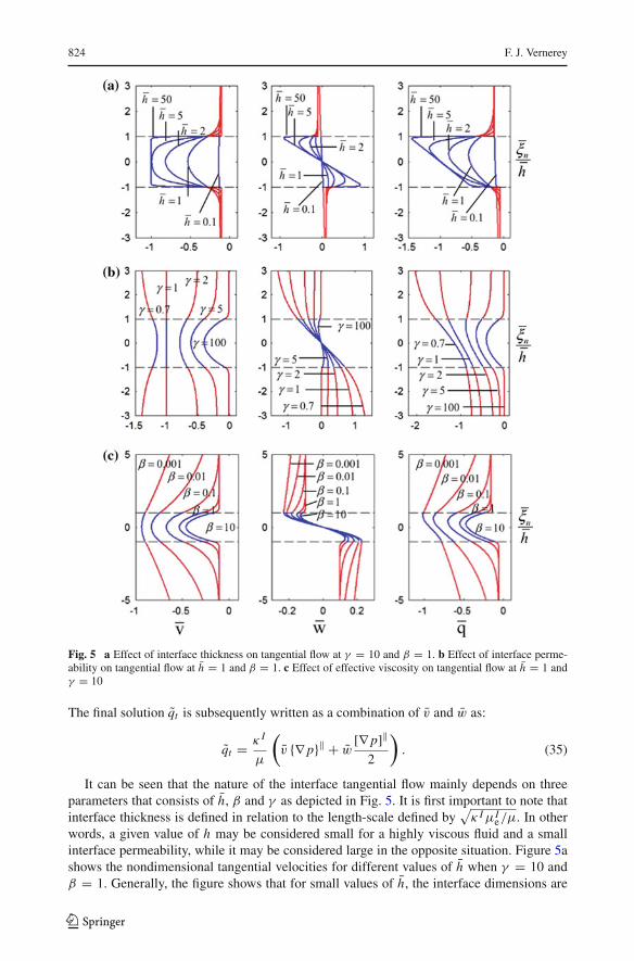
Fig. 5 a Effect of interface thickness on tangential flow at γ = 10 and β = 1. b Effect of interface perme-ability on tangential flow at h = 1 and β = 1. c Effect of effective viscosity on tangential flow at h = 1 andγ = 10

The final solution qt is subsequently written as a combination of v and w as:

qt = κ I

μ

(v {∇ p}‖ + w

[∇ p]‖

2

). (35)

It can be seen that the nature of the interface tangential flow mainly depends on threeparameters that consists of h, β and γ as depicted in Fig. 5. It is first important to note thatinterface thickness is defined in relation to the length-scale defined by

√κ IμI

e/μ. In otherwords, a given value of h may be considered small for a highly viscous fluid and a smallinterface permeability, while it may be considered large in the opposite situation. Figure 5ashows the nondimensional tangential velocities for different values of h when γ = 10 andβ = 1. Generally, the figure shows that for small values of h, the interface dimensions are

123

The Effective Permeability of Cracks and Interfaces 825

too small in order for the tangential flow to fully develop independently from the bulk flow.However, as h increases to values close to unity, interface flow starts developing but is stillconstrained by a transition zone between bulk and interface. However, as h increases to largervalues, the characteristic length of the transition dramatically reduces such that interface andbulk flows become quasi independent at h = 50. These observations are valid for both thesymmetric and antisymmetric parts of the flows, which implies that the development of boththe mean and first moment of interface flow are promoted by large values of h.

The effect of interface permeability, characterized by the ratio γ = κ I /κB is also illus-trated in Fig. 5b for constant interface thickness (h = 1) and effective viscosity ratio (β = 1).As expected, interface flow is slower in the interface for γ < 1 and faster for γ > 1. In addi-tion, as γ increases, the first moment of interface flow can fully develop in the interface, whichtriggers a sharp flow discontinuity across the interface. However, as γ decreases below unity,the interface becomes more resistant to b f qm and the transition region (or boundary layer)mostly occurs in the bulk.

Similarly, the effective viscosity ratio β = μIe/μ

Be plays a large influence on the extend of

the boundary layer near the interface as shown in Fig. 5c. Generally, the extent of the influ-ence of interface flow on bulk flow increases with decreasing β (or increasing bulk viscosityμB

e ).

4 Macroscopic Permeabilities and Their Relation to Microscopic Interface Properties

To bridge micro and macroscopic interface descriptions, we now seek to express macroscopicpermeabilities introduced in (10) and (11) in terms of interface properties h, γ , and β. Thismay be accomplished by projecting the averaging operation defined in (16) along the normaland tangential interface directions and identifying the velocity-pressure relation with (10)and (11).

4.1 Normal permeabilities

Normal macroscopic permeabilities are obtained by projecting (16) onto the normal direction.This yields:

q⊥s = 1

2h

h∫

−h

qndξn = −κI [p]

2μh(36)

q⊥m = 1

4h2

h∫

−h

qnξndξn = −κI I [∇ p]⊥

μ, (37)

where we used (20) to obtain the last terms. Identifying these expressions with (10) and (11)leads to:

κ⊥s = 1 and κ⊥

m = I, (38)

where I was defined in (8), and the above permeabilities are normalized with respect to inter-face permeability κ I , i.e., κ⊥

s = κ⊥s /κ

I and κ⊥m = κ⊥

m /κI . These results show that normal

interface permeabilities are entirely expressed in terms of the microscopic permeability κ I

and are independent of the interface thickness h. This is expected as the fluid viscosity, whichgives rise to size effects, does not play a role in the normal direction.

123

826 F. J. Vernerey

4.2 Tangential permeabilities

In turn, macroscopic tangential permeabilities are obtained by projecting (16) onto the tan-gential direction as follows:

q‖s = 1

2h

h∫

−h

qt dξn = κI {∇ p}‖2hμ

h∫

−h

v dξn (39)

q‖m = 1

4h2

h∫

−h

qtξndξn = κI [∇ p]‖8h2μ

h∫

−h

wξn dξn, (40)

where we implicitly used the expression for qt in (35). Identifying the above equations with(10) and (11), the macroscopic permeabilities are found to be the zeroth and first momentof the symmetric and antisymmetric nondimensional velocities v and w in the interface,respectively:

κ‖s = − 1

2h

h∫

−h

vdξn and κ‖m = − 1

8h2

h∫

−h

wξndξn . (41)

Substituting (31) and (33) into (41) and performing the integration yields the following formsfor the mean tangential permeability:

κ‖s = 1 − β (γ − 1) tanh(h)

h(α + √

α tanh(h)) (42)

and the tangential permeability to the first moment of interface flow:

κ‖m = I −

(hβ (γ − 1)− √

α) (

h coth(h)− 1)

4h3(α + √α coth(h))

. (43)

These two relationships, together with (38) are the main results of this article. Theyindeed provide a clear relation between macroscopic permeabilities and microscopic inter-face parameters. To better understand these findings, Fig. 6 provides an illustration of thevariation of macroscopic tangential permeabilities in terms of changes in microscopic inter-face properties. Thus, Fig. 6a shows that mean permeability κ‖

s varies nonlinearly from beingequal to the bulk permeability κB when h = 0, to being equal to the interface permeabilityκ I when h becomes large compared to unity. Similarly, the permeability κ‖

m varies from 0when h = 0, to Iκ I for large values of h. In other words, thin interfaces (h → 0) tend toprohibit any flow q‖

m in comparison to thicker ones. An interesting feature is the existenceof an optimum value of h (around 1) for which κ‖

m reaches a maximum when γ < 1. Thisphenomenon may be explained as follows; for large values of h, interface flow is totallyindependent from that in the bulk and the value of κ‖

m approaches that of an infinitely thickinterface κ‖

m = Iκ I . However, when h ≈ 1, significant interactions exist between bulk flowand interface flow; the fast bulk flow tends to increase the first moment of interface fluidvelocity in the interface due to viscous interactions (right figure in Fig. 6a). The consequenceis an increased value of κ‖

m for intermediate values of h.The influence of interface permeability ratio γ is then assessed on macroscopic proper-

ties as depicted in Fig. 6b. Results show that both κ‖s and κ‖

m are decreasing functions of γ .

123

The Effective Permeability of Cracks and Interfaces 827

Fig. 6 a Effect of interface thickness effective permeabilities κ‖s and κ‖

m . For all cases, β = 1. Note that the

permeability κ‖m exhibits a maximum around h = 1 when γ < 1. This can be explained in terms of velocity

ratios as shown in the last figure for γ = 0.2 and β = 1. It can clearly be seen that the maximum flow q‖m

is observed when h = 1. b Effect of permeability ratio γ on effective permeabilities. For all cases, β = 1.c Effect of viscosity ratio β on effective permeabilities. For all cases, β = 1

When γ > 1, mean interface velocity is decreased by the slower bulk velocity due to viscousinteractions as shown in the last figure of Fig. 6b. This phenomenon tends to decrease themean tangential permeability. The opposite effect can be observed when γ < 1. In this case,bulk velocity is larger than interface velocity and this tends to increase tangential perme-abilities. It should be noted that as the interface thickness becomes larger, these interactionsbecome negligible as dragging effects between bulk and interface vanish. This explains why

123

828 F. J. Vernerey

for large thickness (h → ∞), the curves converges to horizontal lines corresponding toκ

‖s = κ I and κ‖

m = Iκ I .Finally, Fig. 6c illustrates the role of permeability ratio β = μI

e/μBe on bulk/interface

interactions. Generally, as β increases, the effect of bulk velocity on interface permeabilitiesbecomes more and more pronounced. This generally tends to increase κ‖ when γ < 1 (i.e.,when bulk velocity is larger than interface velocity) and decrease κ‖ when γ > 1 (i.e., whenbulk velocity is smaller than interface velocity).

5 Concluding Remarks

In summary, this article proposed to investigate the macroscopic properties of interfaces inporous media in terms of the microscopic properties, including thickness, permeability, andeffective Brinkman viscosity. In particular, the major contribution of this work was to analyt-ically derive relationships between interface permeabilities and microscopic properties andfeatures in the context of the incompressibility and isotropy of the fluid and porous medium.We found that macroscopic tangential permeabilities are strongly affected by boundary lay-ers developing at the boundary between bulk and interface domains. The size and nature ofthese layers were in turn strongly affected by interface thickness, permeability and effectiveviscosity. More specific findings can be stated as follows:

• The normal permeabilities are independent of interface thickness and only depend onthe microscopic interface permeabililty κ I .

• The mean tangential permeability is bounded between bulk permeability (for very thininterfaces) and interface permeability κ I (for thick interfaces).

• The tangential permeability to the first moment of interface velocity varies between zero(for very thin interfaces) and Iκ I (for thick interfaces). However, it reaches a maximumaround h = 1, in the case where κ I < κB.

In addition to providing a better understanding of fluid flow in porous interfaces, resultsreported in this article will enable the macroscopic modeling of interfaces in porous media asline discontinuity of zero thickness while keeping an accurate description of the microscopicproperties through interface permeability definitions. This capability will prove useful in avariety of problems including soils mechanics, the mechanics of fractured porous media,fluid flow in biological media with interfaces and the mechanics of biological cells (Vernereyand Farsad 2011a; Farsad et al. 2010).

Acknowledgments The author gratefully acknowledges the National Science Foundation, Grant No. CMMI-0900607 and the National Institute of Health, Grant No. 1R21AR061011 in support of this work.

References

Barthelemym, J.F.: Effective permeability of media with a dense network of long and micro fractures. Transp.Porous Media 76, 153–178 (2009)

Biot, M.A.: General theory of three-dimensional consolidation. J. Appl. Phys. 12, 155–164 (1941)Biot, M.A.: The elastic coefficients of the theory of consolidation. J. Astrophys. Astron 24, 594–601 (1957)Bowen, R.M.: Incompressible porous media models by the use of the theory of mixtures. Int. J. Eng.

Sci. 18, 1129–1148 (1980)Chandesris, M., Jamet, D.: Boundary conditions at a planar fluid–porous interface for a poiseuille flow. Int. J.

Heat Mass Transf. 49(13–14), 2137–2150 (2006)

123

The Effective Permeability of Cracks and Interfaces 829

Dormieux, L., Kondo, D.: Approche micromecanique du couplage permeabilite-endommagement. ComptesRendus Mecanique 332, 135–140 (2007)

Farsad, M., Vernerey, F.J., Park, H.: An extended finite element/level set method to study surface effects on themechanical behavior and properties of nanomaterials. Int. J. Numer. Methods Eng. 84, 1466–1489 (2010)

Ghabezloo, S., Pouya, A.: Numerical upscaling of the permeability of a randomly cracked porous medium.In: The 12th International Conference of International Association for Computer Methods and Advancesin Geomechanics (IACMAG) (2008)

Goyeaua, B., Lhuillierb, D., Gobina, G., Velardec, M.: Momentum transport at a fluid–porous interface. Int.J. Heat Mass Transf. 46(21), 4071–4081 (2003)

Gurtin, M.E., Weissmuller, J., Larche, F.: A general theory of curved deformable interfaces in solids at equi-librium. Philos. Mag. A 78, 1093–1109 (1998)

Liolios, P.A., Exadaktylos, G.E.: A solution of steady-state fluid flow in multiply fractured isotropic porousmedia. Int. J. Solids Struct. 43, 3960–3982 (2008)

Pouya, A., Ghabezloo, S.: Flow-stress coupled permeability tensor for fractured rock masses. Transp. PorousMedia 32, 1289–1309 (2008)

Sun, D.N., Gu, W.Y., Guo, X.E., Lai, W.M., Mow, V.C.: A mixed finite element formulation of triphasicmechano-electromechanical theory for charged, hydrated biological soft tissues. Int. J. Numer. MethodsEng. 45, 1375–1402 (1999)

Truesdell, C.: Rational Thermodynamics. McGraw-Hill Series in Modern Applied Mathematics. McGraw-Hill, New York (1969)

Vernerey, F.J.: On the mechanics of interfaces in deformable porous media. Int. J. Solids Struct. doi:10.1016/j.ijsolstr.2011.07.005 (2011)

Vernerey, F.J., Farsad, M.: A constrained mixture approach to mechano-sensing and force generation incontractile cells. J. Mech. Behav. Biomed. Mater. doi:10.1016/j.jmbbm.2011.05.022 (2011a)

Vernerey, F.J., Farsad, M.: An eulerian/xfem formulation for the large deformation of cortical cell membrane.Comput. Methods Biomech. Biomed. Eng. 14, 433–445 (2011b)

Vernerey, F.J., Foucard, L., Farsad, M.: Bridging the scales to explore cellular adaptation and remodeling.Bionanoscience. doi:10.1007/s12668-011-0013-6 (2011a)

Vernerey, F.J., Greenwald, E., Bryant, S.J.: Triphasic mixture model of cell-mediated enzymatic degradationof hydrogels. Comput. Methods Biomech. Biomed. Eng. doi:10.1080/10255842.2011.585973 (2011b)

123