the effect of manganese, nitrogen and molybdenum on the corrosion
TRANSCRIPT
The Effect of Manganese, Nitrogen and Molybdenumon the Corrosion Resistance of a Low Nickel (<2 wt%)
Austenitic Stainless Steel
By
Asimenye Muwila
Submitted in fulfilment of the requirements for the degree
MSc: Materials and Metallurgy Engineering
In the Faculty of Engineering, The School of Process andMetallurgical Engineering, University of the Witwatersrand,
Johannesburg
2006

Declaration
I declare that this dissertation is my own, unaided work. It is beingsubmitted for the Degree of Masters of Science in Materials andMetallurgical Engineering in the University of the Witwatersrand,Johannesburg. It has not been submitted before for any degree orexamination in any other university.
Asimenye Muwila10th day of May 2006
ii
Abstract
This dissertation is a study of the effect of manganese, nitrogen and molybdenum on
the corrosion behaviour of a low nickel, austenitic stainless steel. The trademarked
steel, HerculesTM, has a composition of 10 wt% Mn, 0.05 wt% C, 2 wt% Ni, 0.25
wt% N and 16.5 wt% Cr. Eighteen alloys with a HerculesTM base composition were
made with varying manganese, molybdenum and nitrogen contents, to establish the
effect of these elements on the corrosion behaviour of the steel, and to determine a
composition that would ensure increased corrosion resistance in very corrosive
applications. The manganese was varied in three levels (5, 10 and 15 wt%), the
molybdenum in three levels (0.5, 1 and 2 wt%) while the nitrogen was varied only in
two levels (0.15 and 0.3 wt%).
The dissertation details the manufacturing and electrochemical corrosion testing of
these alloys. Preliminary tests were done on 50g buttons, and full-scale tests on 5 kg
ingots. The buttons had a composition that was not on target, this was however
rectified in the making of the ingots. Potentiodynamic tests were done in a 5 wt%
sulphuric acid solution and the corrosion rate (mm/y) was determined directly from
the scans.
From the corrosion test results, it was clear that an increase in manganese decreases
the corrosion rate, since the 5 wt% Mn alloys had the highest corrosion rate, whereas
the 15 wt% Mn alloys, the lowest.
The addition of molybdenum at 5 wt% Mn decreased the corrosion rate such that a
trend of decreasing corrosion rate with increasing molybdenum was observed. At 10
and 15 wt% Mn molybdenum again decreased the corrosion rate significantly, but the
corrosion rate value remained more or less constant irrespective of the increasing
molybdenum content.
iii
At nitrogen levels lower than those of HerculesTM (less than 0.25 wt%) there was no
change in corrosion rate as nitrogen was increased to levels closer to 0.25 wt%. For
nitrogen levels higher than 0.25 wt%, corrosion rates decreased as nitrogen levels
were increased further from 0.25 wt% but only at Mo contents lower than 1.5 wt%.
The HerculesTM composition was developed for its mechanical properties.
Microstructural analyses revealed that the 5 wt% Mn alloys were not fully austenitic
and since the 15 wt% Mn alloys behave similarly to the 10 wt% Mn alloys, it was
concluded that 10 wt% Mn was optimum for HerculesTM. All the alloys tested had a
much lower corrosion rate than HerculesTM. Any addition of molybdenum thus
improved the corrosion rate of this alloy. An alloy with a HerculesTM base
composition, 10 wt% Mn, 0.15 wt% N and a minimum addition of 0.5 wt% Mo
would be a more corrosion resistant version of HerculesTM.
Pitting tests were done on the 10 wt% Mn ingots in a 3.56 wt% sodium chloride
solution. The results showed that an increase in molybdenum increased the pitting
resistance of the ingots.
Immersion tests in a 5 wt% sulphuric acid solution at room temeperature on the 10
wt% Mn ingots confirmed that the ingots corroded by means of general corrosion.

iv
Acknowledgements
The Lord
Thank you God for all the opportunities that You have afforded me. Without Younone of this would be possible.
My Supervisors
I would like to thank Dr. M. Sephton for her patience, understanding, interest andinvaluable advice. I would also like to thank Mr. R. Paton for his guidance.
Technical Assistance
Thanks to Jonathan Kerr, Joseph Moema, Patrick Mokaleng, Clement Dlamini andEdson Muhuma for sharing their technical knowledge on melting, preparing andexamining samples. Thanks also to Bernard Joja for his SEM expert advice.
Institutions
I would like to thank Mintek for their sponsorship of my undergraduate, as well aspostgraduate studies, and for the use of their facilities at what is now AMD(Advanced Materials Division). Thanks to the School of Process and MaterialsEngineering at the University of the Witwatersrand for allowing me to use theirequipment and providing me with a computer and office space as well as the NRF forsponsoring my postgraduate studies.
Others VIP's
Thanks mum and dad for being so understanding and supportive even when youdisagreed. Thanks Lusu and Ngata for making me laugh when I needed to. Ali andChif thanks for your support. Mwaf - still missing you. Thanks Wes for yourunderstanding and patience.
Table of Contents
v
DECLARATION ........................................................................................................................I
ABSTRACT................................................................................................................................ II
ACKNOWLEDGEMENTS .................................................................................................. IV
1. INTRODUCTION................................................................................................................. 2
2. LITERATURE REVIEW ................................................................................................... 5
2.1 STAINLESS STEELS ................................................................................................5
2.1.1 Type 304 stainless steels ...................................................................................9
2.1.2 Type 201 stainless steels ...................................................................................9
2.1.3 Hercules Alloy .............................................................................................10
2.2 CORROSION RESISTANCE OF STAINLESS STEELS ....................................................11
2.2.1 General corrosion...........................................................................................11
2.2.2 Pitting corrosion .............................................................................................14
2.2.3 Corrosion of control alloys .............................................................................17
2.3 EFFECT OF ALLOYING ELEMENTS ON THE CORROSION BEHAVIOUR OF STAINLESS
STEELS.................................................................................................................18
2.3.1 Effect of chromium..........................................................................................19
2.3.2 Effect of nickel ................................................................................................22
2.3.3 Effect of manganese ........................................................................................24
2.3.4 Effect of molybdenum......................................................................................25
2.3.5 Effect of nitrogen ............................................................................................28
2.4 EFFECT OF MICROSTRUCTURE AND PROCESSING ON THE CORROSION BEHAVIOUR OF
STAINLESS STEELS..............................................................................................34
3. PRODUCTION OF THE ALLOYS .............................................................................. 37

Table of Contents
vi
3.1 GENERAL ...........................................................................................................37
3.2 MELTING PROCEDURE .........................................................................................39
3.2.1 The 50g buttons...............................................................................................39
3.2.2 The 5kg ingots.................................................................................................42
3.2.3 Results of chemical analysis for the buttons and ingots ...................................43
3.2.4 Rolling and heat treatment ..............................................................................47
3.2.4.1 The 50g buttons............................................................................................47
3.2.4.2 The 5kg ingots..............................................................................................47
3.3. MICROSTRUCTURES OF THE ALLOYS ........................................................... 48
3.3.1 Predicting the microstructure..........................................................................48
3.4 ACTUAL MICROSTRUCTURE.................................................................................52
3.4.1 Optical microscopy .........................................................................................52
3.4.2 Hardness tests.................................................................................................55
4. EFFECT OF ALLOYING ELEMENTS ON CORROSION BEHAVIOUR OF
HERCULES-BASED ALLOYS ................................................................................. 57
4.1 TESTING PROCEDURE FOR GENERAL CORROSION ..................................................57
4.2 RESULTS OF CORROSION TESTS............................................................................59
4.2.1 Calculating corrosion rate ..............................................................................60
4.2.2 Corrosion rate as a function of Mn, N and Mo content....................................62
4.2.3 Passivation current density (ipass) of the alloys ................................................65
4.2.4 Critical current density (icrit) of the alloys .......................................................66
4.3 DISCUSSION AND CONCLUSIONS ..........................................................................69
5. THE 10WT% MANGANESE INGOTS ...................................................................... 71
Table of Contents
vii
5.1 GENERAL CORROSION OF 10 WT% MN INGOTS ....................................................71
5.2 PITTING CORROSION TESTS OF 10 WT% MN INGOTS .............................................75
5.2.1 Pitting resistance equivalent (PRE) for the 10 wt% alloys...............................75
5.2.2 Cyclic potentiodynamic polarization testing of the 10 wt% Mn ingots .............76
5.3 IMMERSION TESTS OF 10WT % MN INGOTS ..........................................................78
5.3.1 Results of immersion tests ...............................................................................79
5.3.2 SEM analysis of ingots 7-9..............................................................................82
5.4 DISCUSSION AND CONCLUSIONS..........................................................................83
6. SUMMARY AND CONCLUSIONS ............................................................................. 84
7. REFERENCES .................................................................................................................... 89
APPENDICES .......................................................................................................................... 96
List of Figures
viii
Figure 2. 1: The iron-chromium (Fe-Cr) phase diagram [Peckner and Bernstein,
1977;Honeycombe,1981]. .......................................................................5
Figure 2. 2: Schaeffler diagram [Peckner and Bernstein, 1997; Lula,1986] .........7
Figure 2. 3: Anodic polarization curve of stainless steel in sulphuric acid solution
[Sedriks, 1986] ......................................................................................12
Figure 2. 4: Autocatalytic process occurring in a corrosion pit [Fontana and
Greene, 1982]. .......................................................................................16
Figure 2. 5: Effect of chromium content of FeNiCr alloys on their anodic
polarisation behaviour in 2N H2SO4 at 90˚C. The nickel content was
in the range of 8.3% to 9.8% [Sedriks, 1986] ......................................20
Figure 2. 6: Effect of chromium content on pitting potential of Fe-Cr alloys in a
deaerated 0.1 N NaCl solution at 25°C [ after Sedriks, 1979].............21
Figure 2. 7: Effect of increasing nickel on two heats of Cr-Ni-Mn steel in 65%
nitric acid [Gross, 1980] .......................................................................22
Figure 2. 8: Effect of nickel on pitting potential of Fe-15%Cr alloys in a
deaerated 0.1 N NaCl solution at 25°C [after Sedriks, 1979]..............23
Figure 2. 9: Effect of manganese content on corrosion of 17.5% Cr, 4% Ni steels
in 65% nitric acid [Gross, 1980]. .........................................................25
Figure 2. 10: Effect of molybdenum content on the anodic polarisation curves of
an Fe-18% Cr alloy in 1N H2SO4 [Gross 1980]. ..................................26
Figure 2. 11: Effect of molybdenum on pitting potential of Fe-15% Cr-13% Ni
alloys in deaerated 0.1N NaCl solution at 25°C [after Sedriks; 1986].
...............................................................................................................27
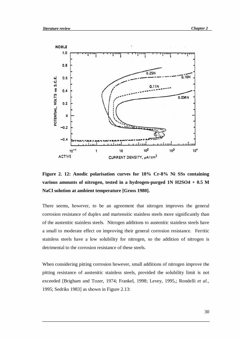
Figure 2. 12: Anodic polarisation curves for 18% Cr-8% Ni SSs containing
various amounts of nitrogen, tested in a hydrogen-purged 1N H2SO4
+ 0.5 M NaCl solution at ambient temperature [Gross 1980]. ............30
List of Figures
ix
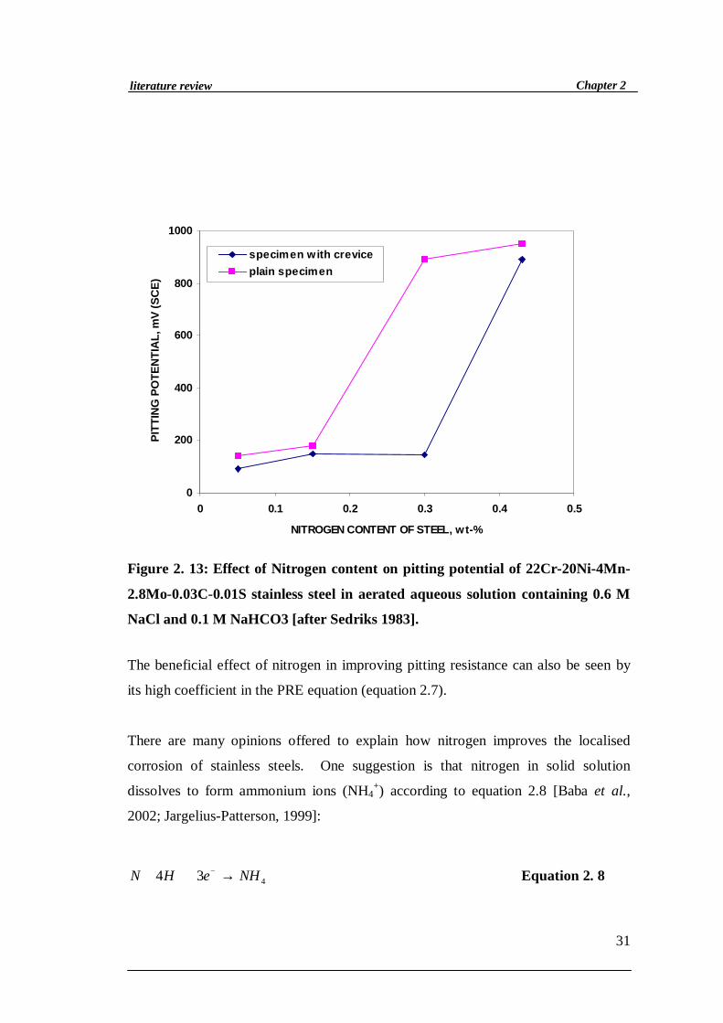
Figure 2. 13: Effect of Nitrogen content on pitting potential of 22Cr-20Ni-4Mn-
2.8Mo-0.03C-0.01S stainless steel in aerated aqueous solution
containing 0.6 M NaCl and 0.1 M NaHCO3 [after Sedriks 1983]. .....31
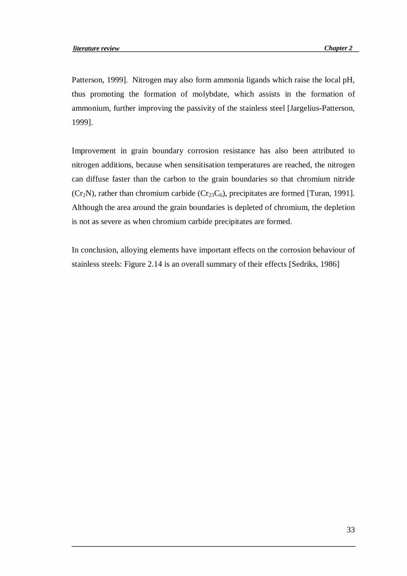
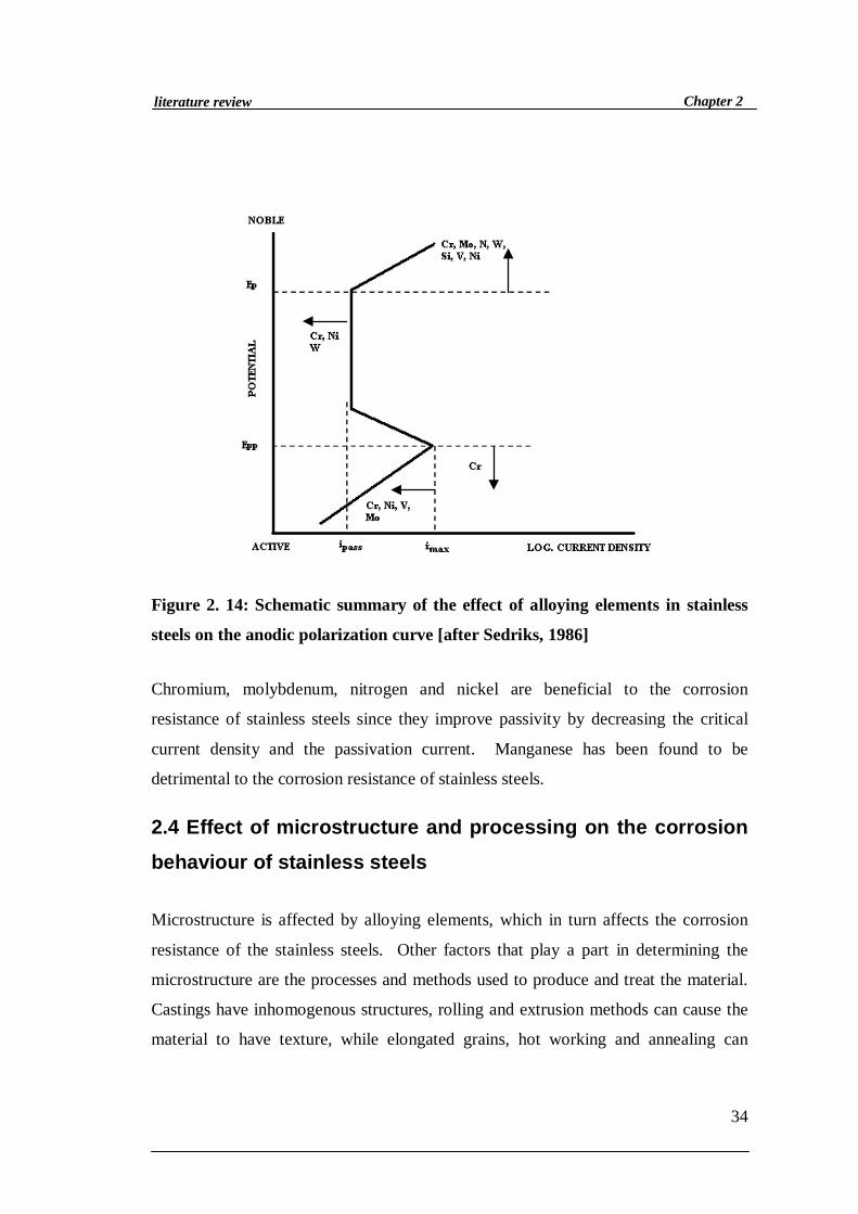
Figure 2. 14: Schematic summary of the effect of alloying elements in stainless
steels on the anodic polarization curve [after Sedriks, 1986]..............34
Figure 3. 1: Average ferritescope readings for the eighteen manufactured
buttons. .................................................................................................40
Figure 3. 2: Average ferritescope readings taken for the nine buttons after
reheating at 1050°C and air cooling.....................................................41
Figure 3. 3: Average ferritescope readings taken for the eighteen manufactured
ingots. ....................................................................................................42
Figure 3. 4: Molybdenum content of buttons and ingots made............................43
44
Figure 3. 5: Manganese content of buttons and ingots made. ..............................44
Figure 3. 6: Nitrogen content of buttons and ingots made. ..................................45
Figure 3. 7: Solubility of nitrogen (wt%) in the liquid phase at 1600ºC and 0.80
atm N2 partial pressure [Kerr, 2003] ...................................................46
Figure 3. 8: Schaeffler diagram for the 5wt% Mn ingots, AISI 201, 304 and
Hercules™ are also indicated here for reference. ...............................49
Figure 3. 9: Schaeffler diagram for the 10wt% Mn ingots, AISI 201, 304 and
Hercules™ are also indicated here for reference. ...............................50
Figure 3. 10: Schaeffler diagram for the 15wt% Mn ingots, AISI 201, 304 and
Hercules™ are also indicated here for reference. ...............................51
Figure 3. 11: Effect of nitrogen on ferrite content of 5kg ingots. .........................53
Figure 3. 12: Effect of manganese on ferrite content of 5kg ingots......................54
List of Figures
x
Figure 3. 13: Effect of molybdenum on ferrite content of 5kg ingots ..................55
Figure 3. 14: Hardness of the 5kg ingots...............................................................56
Figure 4. 1: Example of scans obtained for both ingots and buttons...................59
Figure 4. 2: Evans diagram showing the origin of a cathodic nose [Kerr et al.,
2003]......................................................................................................60
Figure 4. 3: calculation of Rp from the potentiodynamic curve. ..........................61
Figure 4. 4: Corrosion rate of 5 wt% Mn buttons and alloys. .............................62
Figure 4. 5: Corrosion rate of 10 wt% Mn buttons and ingots. ...........................63
Figure 4. 6: Corrosion rate of 15 wt% Mn alloys .................................................64
Figure 4. 7: ipass for the buttons and ingots. ..........................................................65
Figure 4. 8: icrit for the buttons and ingots. ...........................................................66
Figure 4. 9: icrit for the buttons at 5, 10 and 15wt% Mn buttons. ........................67
Figure 4. 10: Ingots 5 and 10 wt% Mn .................................................................68
Figure 5. 1: A typical scan obtained during testing of ingots 7 to 12, showing
very good reproducibility. ....................................................................72
Figure 5. 2: Corrosion rate for ingots 7 to 12 as a function of Mo content..........73
Figure 5. 3: Full potentiodynamic scans of ingots 7 to 12 in 5 wt% H2SO4.........74
Figure 5. 4: PRE values for ingots 7to 12..............................................................76
Figure 5. 5: Example of cyclic scan obtained from pitting tests...........................77
Figure 5. 6: Pitting potentials of alloys 7-12, as well as Hercules, AISI 304 and
201. ........................................................................................................78
Figure 5. 8: Corrosion rate of ingots 7-12 after immersion tests. ........................81
Figure 5. 9: SEM (SEI) image of ingot 9 at X1100. ..............................................82
List of Tables
xi
Table 1. 1: Prior art austenitic stainless steels with reduced contents of nickel[Cortie, 1995]……………………………………………………………3
Table 1. 2: Possible applications for Hercules and the corrosion attackcommon to these applications………………………………………….5
Table 2. 1: General composition of AISI type 304 stainless steels [Harvey, 1982].9
Table 2. 2: General chemical composition of AISI type 201 stainless steel[Harvey, 1982]…………………………………………………………10
Table 2. 3: Chemical composition of Hercules alloy……………………………10
Table 3. 1: Matrix of alloys that were made………………………………………38
Table 3. 2: Etchants used for electro-etching……………………………………..52
Table 4. 1: Testing procedure for general corrosion of the alloys……………….58
Chapter 1
2
1. Introduction
Nickel prices are notorious for being high and unstable and since austenitic stainless
steels contain 8-10% nickel, price instability strongly affects the stainless steel
industry. Nickel prices fluctuate because nickel is expensive to process and is not
always readily available [Rama Rao and Kutumbarao, 1989]. The cost of nickel is
currently averaging at $15000/tonne and is expected to increase [Moema et al., 2005].
This has once again sparked interest in the development of a low nickel austenitic
stainless steel.
Reducing the nickel content in austenitic stainless steels significantly reduces their
price. Nickel’s ability to stabilise and form austenite is, however, an integral part in
the processing of austenitic stainless steels, and if the nickel content is to be reduced
appreciably, other austenite forming elements, such as carbon, nitrogen, manganese
and copper, need to be used for the partial or complete replacement of nickel [Kerr,
2003; Lula, 1986]. These elements have the advantage of costing less than nickel.
There has been much research into replacing Ni with other austenizing elements
[Lula, 1986; Turan, 1991]. Nickel shortages before World War II in Europe and in
the United States during the Korean War initiated the replacement of nickel in
austenitic stainless steels with manganese and nitrogen [Lula, 1986; Sedriks, 1979].
This led to the development of the now standard and commercial AISI 200 Series
stainless steels. These steels are not, however, as popular as the 304 type steels
because of their high tensile strength, hardness and work hardening rate, which make
them difficult to form and they have poor corrosion resistance [Sedriks, 1979]. Other
3
Chapter1
introduction
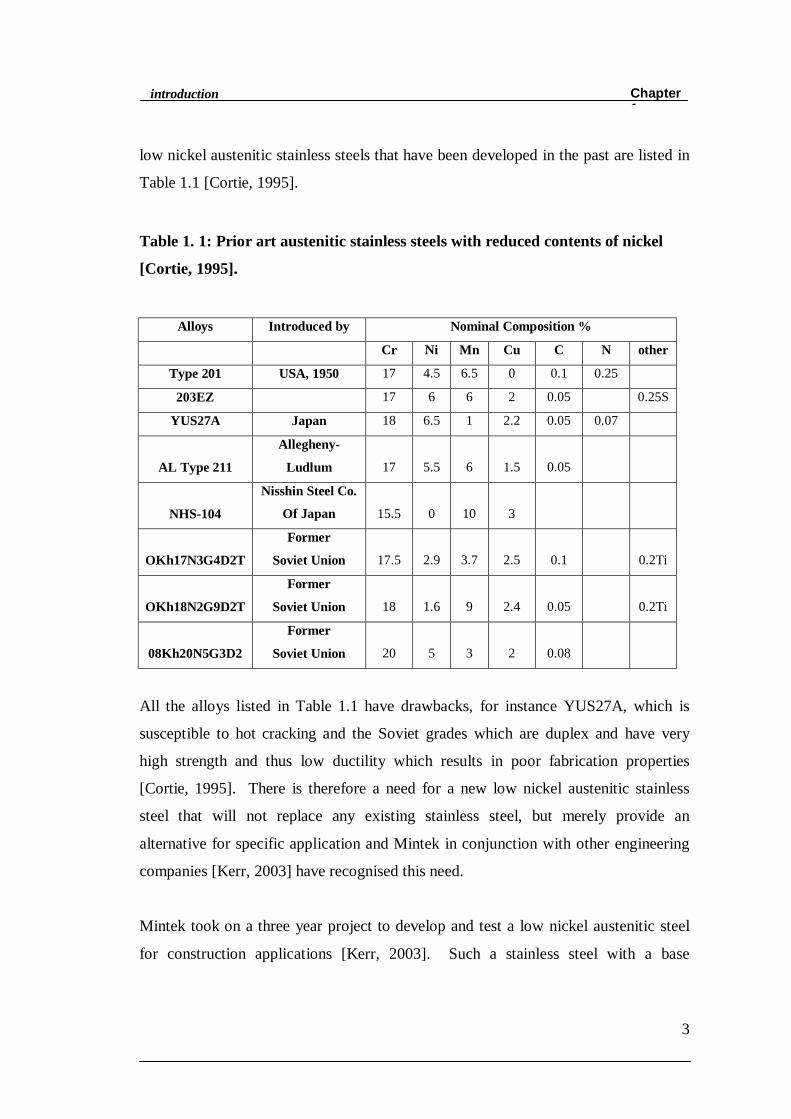
low nickel austenitic stainless steels that have been developed in the past are listed in
Table 1.1 [Cortie, 1995].
Table 1. 1: Prior art austenitic stainless steels with reduced contents of nickel
[Cortie, 1995].
Alloys Introduced by Nominal Composition %
Cr Ni Mn Cu C N other
Type 201 USA, 1950 17 4.5 6.5 0 0.1 0.25
203EZ 17 6 6 2 0.05 0.25S
YUS27A Japan 18 6.5 1 2.2 0.05 0.07
AL Type 211
Allegheny-
Ludlum 17 5.5 6 1.5 0.05
NHS-104
Nisshin Steel Co.
Of Japan 15.5 0 10 3
OKh17N3G4D2T
Former
Soviet Union 17.5 2.9 3.7 2.5 0.1 0.2Ti
OKh18N2G9D2T
Former
Soviet Union 18 1.6 9 2.4 0.05 0.2Ti
08Kh20N5G3D2
Former
Soviet Union 20 5 3 2 0.08
All the alloys listed in Table 1.1 have drawbacks, for instance YUS27A, which is
susceptible to hot cracking and the Soviet grades which are duplex and have very
high strength and thus low ductility which results in poor fabrication properties
[Cortie, 1995]. There is therefore a need for a new low nickel austenitic stainless
steel that will not replace any existing stainless steel, but merely provide an
alternative for specific application and Mintek in conjunction with other engineering
companies [Kerr, 2003] have recognised this need.
Mintek took on a three year project to develop and test a low nickel austenitic steel
for construction applications [Kerr, 2003]. Such a stainless steel with a base

4
Chapter1
introduction
composition of 0.02-0.08% carbon, 1.8-2% nickel, 15-17% chromium, 9-10%
manganese, 0.2-0.8% silicon and 0.2-0.3% nitrogen, which has a yield strength
greater than 350MPa has already been produced [Kerr, 2003]. This alloy, called
Hercules, has good mechanical properties but was found, from preliminary tests, to
have poor corrosion resistance. It is believed though that varying the manganese and
nitrogen levels of the Hercules and adding molybdenum will improve its corrosion
resistance.
This project dealt with the investigation of the corrosion resistance of Hercules.
Different alloys with a Hercules base composition but varying manganese, nitrogen
and molybdenum levels were made so that the effect of these elements on the
corrosion resistance of Hercules could be investigated. It is important for its
acceptance in the stainless steel industry that Hercules have comparable corrosion
resistance to popular and standard commercial stainless steels, such as AISI 304 and
201, and one of the aims of this project was to specify, if possible, the composition of
a corrosion resistant variation of Hercules.
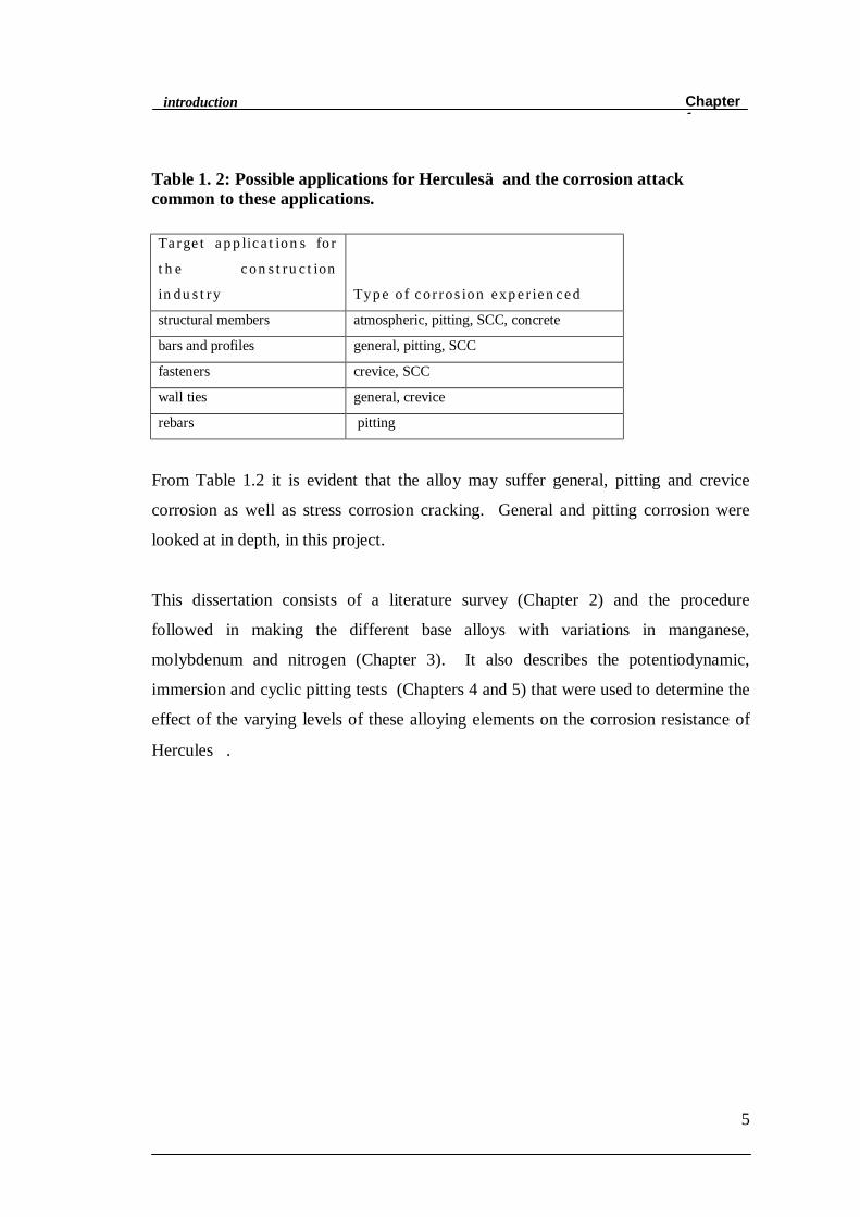
The specific applications for which the new alloy is targeted and the type of corrosion
which it is expected to experience, are listed in Table 1.2.
5
Chapter1
introduction
Table 1. 2: Possible applications for Hercules and the corrosion attackcommon to these applications.
Target applications forthe constructionindustry Type of corrosion experiencedstructural members atmospheric, pitting, SCC, concrete
bars and profiles general, pitting, SCC
fasteners crevice, SCC
wall ties general, crevice
rebars pitting
From Table 1.2 it is evident that the alloy may suffer general, pitting and crevice
corrosion as well as stress corrosion cracking. General and pitting corrosion were
looked at in depth, in this project.
This dissertation consists of a literature survey (Chapter 2) and the procedure
followed in making the different base alloys with variations in manganese,
molybdenum and nitrogen (Chapter 3). It also describes the potentiodynamic,
immersion and cyclic pitting tests (Chapters 4 and 5) that were used to determine the
effect of the varying levels of these alloying elements on the corrosion resistance of
Hercules.
5
Chapter 2
2. Literature Review
As mentioned in Chapter 1, this project deals with the corrosion behaviour of
austenitic stainless steels, and this literature survey provides information on the
general properties and corrosion behaviour of these steels. The effect of alloying
elements such as nickel, molybdenum, chromium, nitrogen and manganese on
microstructure and corrosion behaviour is also discussed.
2.1 Stainless steels
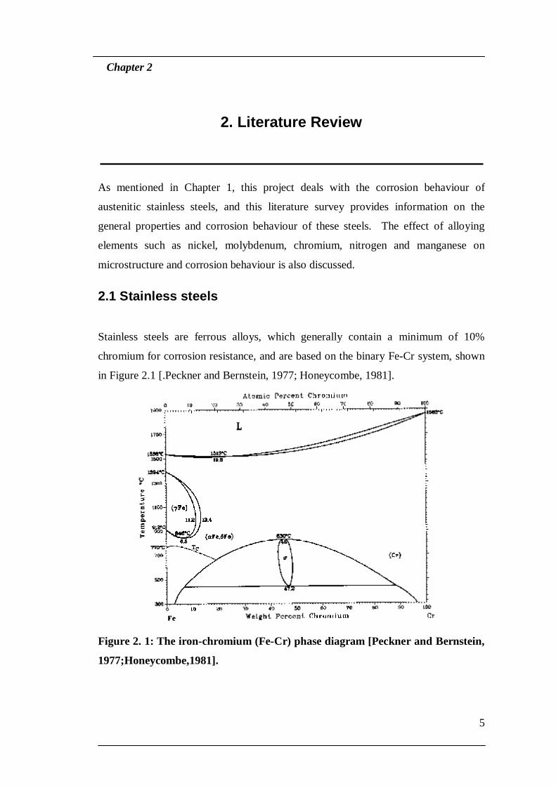
Stainless steels are ferrous alloys, which generally contain a minimum of 10%
chromium for corrosion resistance, and are based on the binary Fe-Cr system, shown
in Figure 2.1 [.Peckner and Bernstein, 1977; Honeycombe, 1981].
Figure 2. 1: The iron-chromium (Fe-Cr) phase diagram [Peckner and Bernstein,
1977;Honeycombe,1981].
6
Chapter 2literature review
This binary Fe-Cr diagram shows the phase transformations that occur in stainless
steels at certain temperatures and compositions. Additions of specific alloying
elements modify this binary system, producing different types of stainless steels such
as martensitic (α’), austenitic (γ), ferritic (α) and duplex. Since chromium is a ferrite
stabiliser, the ferrite (α) phase field on the Fe-Cr phase diagram is extensive while the
austenite (γ) phase field is restricted to a small loop that does not extend beyond 12-
13% chromium and temperatures lower than 800ºC. This austenite loop can,
however, be expanded by the addition of a face centered (FCC) alloying element,
such as nickel or manganese, to the binary Fe-Cr system. If the FCC element is added
in sufficient amounts, the formation of the ferrite (α) phase is suppressed and a fully
austenitic microstructure that is stable at room temperature can be obtained. When
added to steel the atoms of the FCC elements substitute iron atoms in the crystal
lattice [Vismer, 1997]. These FCC atoms diffuse slowly in iron, slowing down the
kinetics needed for ferrite formation. Even though the amount of Ni required to form
and stabilise austenite in steel is variable and is dependent on the ferrite forming
elements, it is generally acceptable that a minimum of 8% nickel is needed to obtain
an austenitic microstructure at room temperature. If, however, other austenite
stabilising or forming elements (nitrogen for instance) are also added to the steel it
may be possible to obtain a fully austenitic structure at room temperature with less
than 8% nickel [Turan, 1991]
Alloying elements can thus be divided into two categories: austenite/ferrite formers
and austenite/ferrite stabilisers. Austenite formers, such as nickel, actually increase
the amount of austenite in the alloy, whereas austenite stabilisers, expand the
austenitic field so that the austenite will be stable at lower temperatures than normal
[Cortie, 1995]. An element can therefore be both an austenite former and stabiliser if
it has the ability to expand the γ - field, so as to encourage the formation of austenite
over wider compositional limits and also stabilise it at lower temperatures.

7
Chapter 2literature review
Ferrite formers, on the other hand, increase the tendency for delta-ferrite formation by
decreasing the austenite loop so that the austenite is unstable and transforms to ferrite
upon cooling [Vismer, 1997]. Delta-ferrite is a BCC (body centered cubic) phase that
is stable between 1394ºC and 1538ºC (melting temperature of steel) [Pickering,
1992]. Delta-ferrite is rich in chromium and other ferrite stabilisers and is undesirable
because it depletes the surrounding matrix of chromium and molybdenum, forming
areas that are susceptible to pitting attack [Sedriks, 1986]. Delta-ferrite can also
transform to hard and brittle sigma phase after long-term exposure at elevated
temperatures, thus decreasing the toughness and ductility of the steel.
The effects of alloying elements on the formation of austenite and ferrite have been
investigated and Schaeffler diagrams, as illustrated in Figure2.2, have been developed
to predict the maximum amount of ferrite (F), austenite (A) and martensite (M) that
can be expected in the microstructure at room temperature in terms of the nickel and
chromium equivalents [Peckner and Bernstein, 1977; Lula, 1986].
Figure 2. 2: Schaeffler diagram [Peckner and Bernstein, 1997; Lula,1986]
8
Chapter 2literature review
Schaeffler diagrams were constructed for predicting weld metal microstructures, but
can be used as a guide when trying to predict if a certain as cast stainless steel will be
fully austenitic at room temperature. The nickel and chromium equivalents have been
determined using the most common austenite and ferrite forming elements
respectively, as in equation 2.1 and equation 2.2 [Peckner and Bernstein, 1977].
Chromium equivalent = (%Cr) + 2(%Si) + 1.5(%Mo) + 5(%V) + 5.5(%Al) +
1.75(%Nb) + 1.5(%Ti) + 0.75(%W) Equation 2.1
Nickel equivalent = (%Ni) + (%Co) + 0.5(%Mn) + 0.3(%Cu) + 30(%C) + 25(%N)
Equation 2.2
Values in the above equations are in weight percentages. The austenite forming
elements contribute towards the nickel equivalent and the ferrite forming elements to
the chromium equivalent.
Depending on composition, the austenite formed in steel may be stable or metastable.
Metastable austenite transforms to martensite either by quenching to temperatures
below Ms (martensite start temperature) or by deformation at temperatures below Md
(temperature below which martensite forms due to plastic deformation) [Vismer,
1997]. The austenite stabilising effect of an element depends on its ability to depress
the Ms and Md temperatures. The Ms temperature is calculated as shown in equation
2.3 [Peckner and Bernstein, 1977; Vismer, 1997].
Ms = 502 – 810(%C) – 1230(%N) – 13(%Mn) – 30(%Ni) – 12(%Cr) – 54(%Cu) –
46(%Mo) Equation 2.3
From the coefficients of N and C in the Ms equation it is evident that these elements
significantly reduce the Ms temperature.
9
Chapter 2literature review
It is desirable to have a stable austenitic microstructure because it is easily weldable,
tough and has better corrosion resistance than ferritic or martensitic microstructures.
This is why the austenitic stainless steels are the largest group of stainless steels used
today [Rama Rao and Kutumbarao, 1989; Sedriks, 1979]. These steels, classified as
the AISI 200 and 300 series [Cortie, 1995; Peckner and Bernstein, 1977], are of
interest to this project, since the AISI 304 and 201 along with the Hercules were
used as control alloys during corrosion testing (refer to chapter 4 and 5).
2.1.1 Type 304 stainless steels
Type 304 steels are general-purpose chromium-nickel stainless steels that have good
corrosion resistance and good formability [Harvey, 1982; Sedriks, 1979]. Type 304L
is a low carbon version of 304 and has similar corrosion behaviour, but superior
intergranular corrosion resistance. Table 2.1 lists the typical compositions of type
304 steels.
Table 2. 1: General composition of AISI type 304 stainless steels in wt%
[Harvey, 1982]
ElementAlloy Cr Ni Fe C(Max) Mn(Max) S(Max) P(Max)AISI304 18-20 8-10.5 bal. 0.08 2 0.5 0.045AISI304L 18-21 8-12.5 bal. 0.03 2 0.03 0.045
These steels can easily be drawn and formed because of their high ductility and good
strength [Harvey, 1982].
2.1.2 Type 201 stainless steels
Type 201 steels, as mentioned before, are part of the AISI type 200 stainless steel
series (austenitic chromium-nickel-manganese stainless steels) that were developed in
10
Chapter 2literature review
the 1950’s because of nickel shortages at that time [Lula, 1986; Sedriks, 1979].
These steels have a general chemical composition as listed in Table 2.2 [Harvey,
1982]
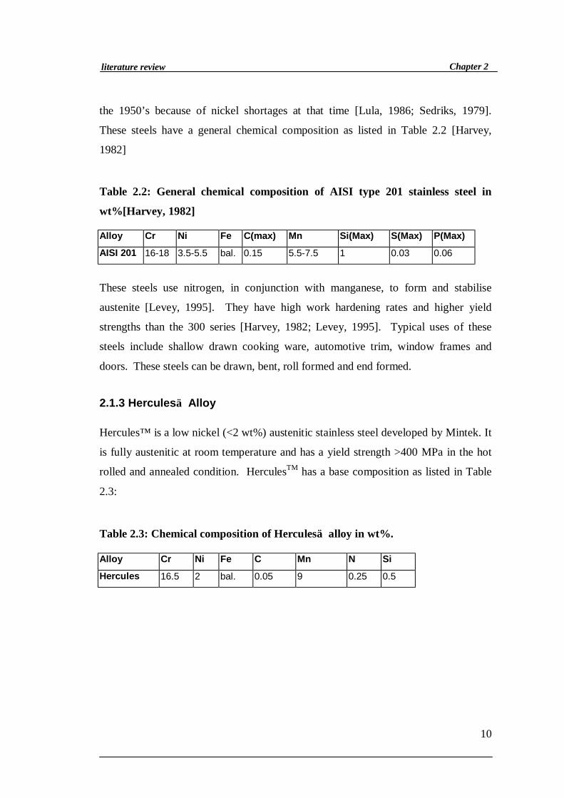
Table 2.2: General chemical composition of AISI type 201 stainless steel in
wt%[Harvey, 1982]
Alloy Cr Ni Fe C(max) Mn Si(Max) S(Max) P(Max)
AISI 201 16-18 3.5-5.5 bal. 0.15 5.5-7.5 1 0.03 0.06
These steels use nitrogen, in conjunction with manganese, to form and stabilise
austenite [Levey, 1995]. They have high work hardening rates and higher yield
strengths than the 300 series [Harvey, 1982; Levey, 1995]. Typical uses of these
steels include shallow drawn cooking ware, automotive trim, window frames and
doors. These steels can be drawn, bent, roll formed and end formed.
2.1.3 Hercules Alloy
Hercules™ is a low nickel (<2 wt%) austenitic stainless steel developed by Mintek. It
is fully austenitic at room temperature and has a yield strength >400 MPa in the hot
rolled and annealed condition. HerculesTM has a base composition as listed in Table
2.3:
Table 2.3: Chemical composition of Hercules alloy in wt%.
Alloy Cr Ni Fe C Mn N Si
Hercules 16.5 2 bal. 0.05 9 0.25 0.5
11
Chapter 2literature review
2.2 Corrosion resistance of stainless steels
2.2.1 General corrosion
Stainless steels have excellent corrosion resistance because they are able to form a
very thin, passive layer of chromium oxide (Cr2O3) that protects them against
corrosive environments [Kincer and McEwan, 1993; Peckner and Bernstein, 1977;
Pickering, 1979; Sedriks, 1986]. This film forms in the presence of oxidising agents,
and is protective in that it has the ability to self-heal in a variety of environments
[Colombier and Hochman, 1965; Newman, 2001; Sedriks, 1979]. Opinions differ on
how the passive film protects stainless steels [Raja et al., 1999]; some authors state
that chromium-oxy-hydroxide (Cr-O-OH) is formed instead of chromium oxide and
that the Cr-O-OH has better protective properties than the Cr2O3 [Hashmito and
Asami, 1979]. Nevertheless the film is essential in maintaining the corrosion
resistance of stainless steels.
When stainless steel is protected by the oxide film it is said to be in a passive state as
it is not experiencing accelerated corrosion. [Sedriks, 1986]. The corrosion behaviour
of stainless steels is known as active-passive behaviour and can be measured using
electrochemical methods. Measurements of the corrosion of stainless steels produce
characteristic anodic polarization curves that reveal the general and localised
corrosion behaviour of these steels. A typical anodic polarisation curve of stainless
steel in sulphuric acid has been redrawn from Sedriks [1986] and is illustrated in
Figure 2.3:
12
Chapter 2literature review
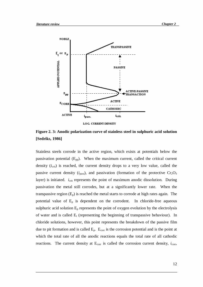
Figure 2. 3: Anodic polarization curve of stainless steel in sulphuric acid solution
[Sedriks, 1986]
Stainless steels corrode in the active region, which exists at potentials below the
passivation potential (Epp). When the maximum current, called the critical current
density (icrit) is reached, the current density drops to a very low value, called the
passive current density (ipass), and passivation (formation of the protective Cr2O3
layer) is initiated. icrit represents the point of maximum anodic dissolution. During
passivation the metal still corrodes, but at a significantly lower rate. When the
transpassive region (Ep) is reached the metal starts to corrode at high rates again. The
potential value of Ep is dependent on the corrodent. In chloride-free aqueous
sulphuric acid solution Ep represents the point of oxygen evolution by the electrolysis
of water and is called Et (representing the beginning of transpassive behaviour). In
chloride solutions, however, this point represents the breakdown of the passive film
due to pit formation and is called Ep. Ecorr is the corrosion potential and is the point at
which the total rate of all the anodic reactions equals the total rate of all cathodic
reactions. The current density at Ecorr is called the corrosion current density, icorr,

13
Chapter 2literature review
which is a measure of corrosion rate since it is directly proportional to metal
dissolution [Jones, 1996; Peckner and Bernstein, 1977; Trethewey and Chamberlain,
2002, Vismer 1997]. icorr cannot be measured directly but with the use of a counter
electrode, reference electrode and a potentiostat it can be determined indirectly
[Jones, 1996]. From the polarisation curve icorr can be determined using either Tafel
extrapolation or polarization resistance1.
icorr values can be converted into mm/y by using Faraday’s Law, which relates current
flow (I) to mass reacted (m) in an electrochemical reaction as in equation 2.4 [Jones
1996].
nFItam = Equation 2. 4 [Jones, 1996]
Where F is Faraday’s constant (96500 coulombs/equivalent), n is the number of
electrons transferred during the reaction, a is the atomic weight and t, the time.
Dividing equation 2.4 through by t, the surface area (A) and density (D), yields a
formula, as in equation 2.5, that can find corrosion rate (r) in mm/y if the current
density is known.
)/(00327.0 yrmmnDair = Equation 2. 5 [Jones, 1996]
Equations 2.4 and 2.5 are valid for pure metals only. For an alloy the determination
of the equivalent weight (a/n in equation 2.5) is required. The equivalent weight
(EW) of an alloy is the weighted average of a/n of the major alloying elements in the
alloy as calculated with equation 2.6 [Jones, 1996].
1 Full explanation of the Tafel extrapolation and polarization resistance methods can be found in Jones,1996. Pp 143-165.
14
Chapter 2literature review
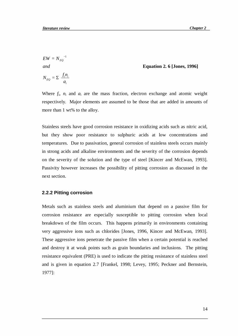
Σ=
= −
i
iiEQ
EQ
anfN
andNEW 1
Equation 2. 6 [Jones, 1996]
Where fi, ni and ai are the mass fraction, electron exchange and atomic weight
respectively. Major elements are assumed to be those that are added in amounts of
more than 1 wt% to the alloy.
Stainless steels have good corrosion resistance in oxidizing acids such as nitric acid,
but they show poor resistance to sulphuric acids at low concentrations and
temperatures. Due to passivation, general corrosion of stainless steels occurs mainly
in strong acids and alkaline environments and the severity of the corrosion depends
on the severity of the solution and the type of steel [Kincer and McEwan, 1993].
Passivity however increases the possibility of pitting corrosion as discussed in the
next section.
2.2.2 Pitting corrosion
Metals such as stainless steels and aluminium that depend on a passive film for
corrosion resistance are especially susceptible to pitting corrosion when local
breakdown of the film occurs. This happens primarily in environments containing
very aggressive ions such as chlorides [Jones, 1996, Kincer and McEwan, 1993].
These aggressive ions penetrate the passive film when a certain potential is reached
and destroy it at weak points such as grain boundaries and inclusions. The pitting
resistance equivalent (PRE) is used to indicate the pitting resistance of stainless steel
and is given in equation 2.7 [Frankel, 1998; Levey, 1995; Peckner and Bernstein,
1977]:
15
Chapter 2literature review
PRE = (%Cr) + 3.3(%Mo) + 16(%N) Equation 2. 7
This equation has been developed to explain the influence of alloying elements on the
pitting resistance of stainless steels. The higher the pitting resistance of an alloy, the
more resistant it is to pitting corrosion. [McEwan, 1994]. The PRE equation has
limitations because it only considers the effect of molybdenum, nitrogen and
chromium on the pitting resistance of stainless steel and the effects of microstructure
on pitting are ignored [McEwan, 1994].
As mentioned, for pitting to occur on stainless steels the presence of aggressive ions
is needed [Schollenberger, 1995]. These ions in most cases are chloride ions from
salt solutions or from chloride bearing compounds such as hypochlorites. The
presence of an oxidising agent, such as oxygen, cupric or ferric ions, that can
maintain passivity on the surface surrounding the pit is also necessary. Low pH
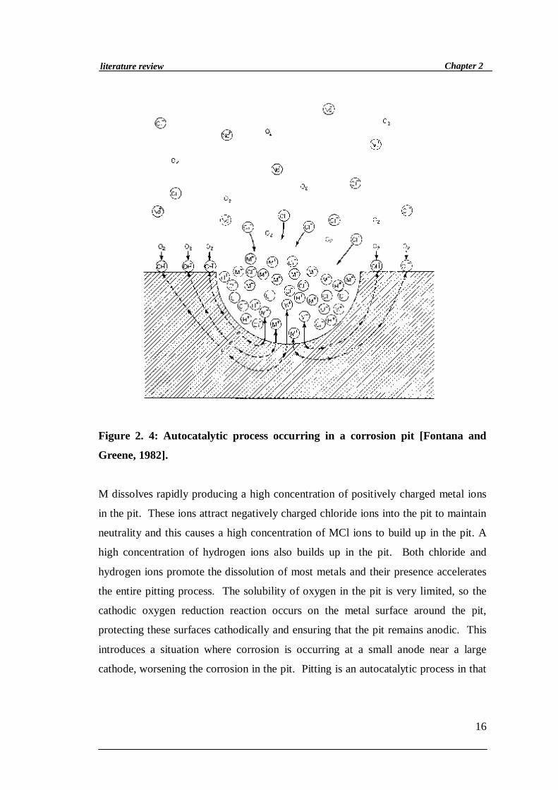
values and static conditions further promote pit formation. Figure 2.4 is an
illustration of the pitting process where metal M is being pitted by an aerated sodium
chloride solution:
16
Chapter 2literature review
Figure 2. 4: Autocatalytic process occurring in a corrosion pit [Fontana and
Greene, 1982].
M dissolves rapidly producing a high concentration of positively charged metal ions
in the pit. These ions attract negatively charged chloride ions into the pit to maintain
neutrality and this causes a high concentration of MCl ions to build up in the pit. A
high concentration of hydrogen ions also builds up in the pit. Both chloride and
hydrogen ions promote the dissolution of most metals and their presence accelerates
the entire pitting process. The solubility of oxygen in the pit is very limited, so the
cathodic oxygen reduction reaction occurs on the metal surface around the pit,
protecting these surfaces cathodically and ensuring that the pit remains anodic. This
introduces a situation where corrosion is occurring at a small anode near a large
cathode, worsening the corrosion in the pit. Pitting is an autocatalytic process in that
17
Chapter 2literature review
as long as there are enough chlorides in the pit preventing repassivation, and provided
the oxidizing agent keeps the surrounding cathodic surface passivated, the pit will
grow. [Fontana and Greene, 1982; Jones, 1996; Schollenberger, 1995].
Manganese sulphides are a major cause of pitting corrosion in manganese bearing
stainless steels. Sulphides form from sulphur that is present as an impurity or an
intentional addition to the steel to improve machinability [Sedriks, 1983].
Manganese sulphides dissolve to form H2S in acid solutions, such as those found in
active pits or crevices. It has been suggested that the formation of H2S makes the
formation of passive films more difficult and that it also promotes the breakdown of
the passive film in stainless steel [Sedriks, 1983]. Manganese sulphides in stainless
steels are anodic with respect to the rest of the steel; they will thus corrode when
exposed to a harsh environment, exposing bare metal to pitting attack2. In fact, any
defect in the metal, inclusions or grain boundaries for example, will act as sites for pit
initiation. It is therefore important to try and avoid these when making steel alloys.
The pitting resistance of an alloy can be determined by examining its pitting potential
(Ep) on the anodic polarisation curve. Generally the more noble the Ep value, the
more resistant the alloy is to pitting corrosion [Sedriks, 1979].
2.2.3 Corrosion of control alloys
The three control alloys of concern to this project, as mentioned before, are the AISI
304, AISI 201 and HerculesTM alloys. AISI 304 is the bread and butter of the
stainless steel industry in that it has excellent corrosion resistance in numerous types
of environments. When fully austenitic, the AISI 304 steels are very resistant to
corrosive attack in nitric acids, but moderately resistant to sulphuric acids [Peckner
and Bernstein, 1977]. AISI 304 in 5 wt% sulphuric acid at 25°C has been found to
2 For pitting mechanisms suggesting how manganese sulphide inclusions can initiate pit propagation instainless steels refer to Sedriks, 1983 and Blom and Degerbeck, 1983.

18
Chapter 2literature review
have a corrosion rate of 0.1-1 mm/y [Avesta Sheffield, 1994]. In an environment
containing halogens, AISI 304 steels have poor corrosion resistance.
The AISI 201 steels resist corrosive attack for relatively long periods in industrial and
marine atmospheres, but have poorer corrosion resistance than the AISI 304 stainless
steels [Harvey, 1982]. Researchers have found AISI 201 to have a corrosion rate >1
mm/y in 5 wt% sulphuric acid at room temperature [Avesta Sheffield, 1994].
Preliminary electrochemical tests done on Hercules indicated that it has a higher
corrosion rate than AISI 304, but comparable to 201 in the hot rolled and annealed
condition. Its corrosion rate was found to be 2.8-35 mm/y [Kerr, 2003; Moema and
Papo, 2005]. The higher corrosion rate is probably due to it having a lower
chromium content than AISI 304. Chromium plays an important role in the
formation of the passive layer of stainless steels, as is discussed in the following
section.
2.3 Effect of alloying elements on the corrosion behaviour of
stainless steels
Alloying elements play a significant role in determining the corrosion behaviour of
stainless steels. The most important effects are the increase of corrosion resistance by
the addition of elements such as chromium, nickel and molybdenum, but also a
decrease in corrosion rate by the addition of elements such as sulphur and manganese.
The stability of the passive film formed on austenitic stainless steels is also dependent
on alloy composition in addition to temperature, passivation time and the working
environment [Bastidas et al., 2002].
Copper is another alloying element that has been found to be beneficial to the
corrosion resistance of stainless steels in sulphuric acid environments [Cortie, 1995,
19
Chapter 2literature review
Sibanda et al., 1994], but it will not be considered in this project since it will not be
added to the alloy.
Alloying elements usually work best in conjunction with one another when
improving corrosion behaviour of a metal [Sedriks, 1979]. For example, chromium
alloyed in conjunction with molybdenum gives the best results in terms of corrosion
resistance for austenitic stainless steels. In the next section the effect of chromium
and nickel on corrosion behaviour and microstructure of stainless steels is discussed
along with those of the elements of interest to this project: nitrogen, manganese and
molybdenum.
2.3.1 Effect of chromium
Chromium is the most important alloying element for corrosion resistance because it
forms a large part of the oxide layer (Cr2O3) that protects the stainless steel from
corrosive environments [Frankel, 1998; Lula, 1986; Peckner and Bernstein, 1977;
Raja et al., 1999]. At least 12% chromium is needed for an alloy to be resistant to
corrosion over an extended range of potential, pH and oxidising power [Audouard,
1993; Cortie, 1995]. Increasing the chromium content beyond 12-13wt% can allow
steels to passivate in more aggressive environments [Peckner and Bernstein, 1997;
Vismer, 1997].
Experiments done on Fe-Ni-Cr alloys in a sulphuric acid solution revealed that
increasing the chromium content of the alloy to levels above 12% decreases the ipass
and shifts the Epp (active-passive transition point) towards the active region, thus
expanding the passive region and improving the corrosion resistance of the metal as
illustrated in Figure 2.5 [Sedriks, 1986].

20
Chapter 2literature review
Figure 2. 5: Effect of chromium content of FeNiCr alloys on their anodic
polarisation behaviour in 2N H2SO4 at 90˚C. The nickel content was in the range
of 8.3% to 9.8% [Sedriks, 1986]
The presence of chromium also improves the pitting resistance of stainless steel in
sulphuric acid by hindering the effects of sulphide ions [Hajjaji et al., 1995]: sulphide
ions exist in steel mailnly as manganese sulphides but they can also contain iron and
chromium. Sulphides (manganese sulphides especially), as mentioned in section
2.2.2, are detrimental to the pitting corrosion resistance of stainless steels. Increasing
the chromium content in the steel, however, increases the amount of chromium
present in the sulphides, thus decreasing the amount of manganese in the sulphides.
21
Chapter 2literature review
Chromium-rich sulphides are more resistant to pit nucleation than manganese-rich
sulphides [Hajjaji et al., 1995].
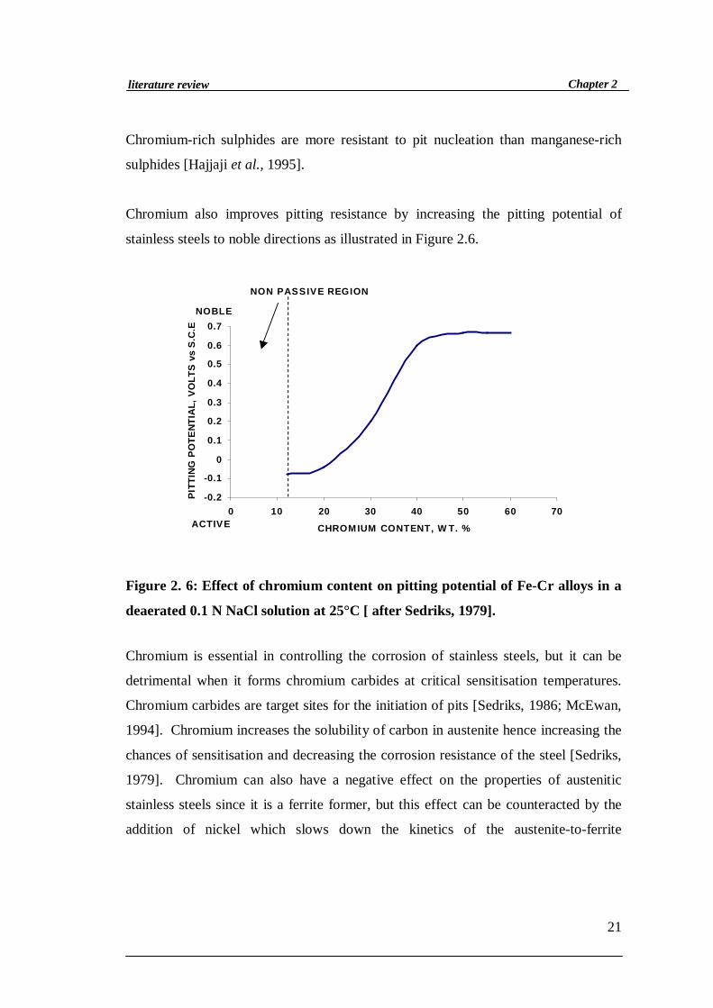
Chromium also improves pitting resistance by increasing the pitting potential of
stainless steels to noble directions as illustrated in Figure 2.6.
NON PASSIVE REGION
-0.2
-0.1
0
0.1
0.2
0.3
0.4
0.5
0.6
0.7
0 10 20 30 40 50 60 70
CHROMIUM CONTENT, W T. %
PIT
TIN
G P
OTE
NTI
AL,
VO
LTS
vs
S.C
.E
ACTIV
NOBLE
ACTIVE
Figure 2. 6: Effect of chromium content on pitting potential of Fe-Cr alloys in a
deaerated 0.1 N NaCl solution at 25°C [ after Sedriks, 1979].
Chromium is essential in controlling the corrosion of stainless steels, but it can be
detrimental when it forms chromium carbides at critical sensitisation temperatures.
Chromium carbides are target sites for the initiation of pits [Sedriks, 1986; McEwan,
1994]. Chromium increases the solubility of carbon in austenite hence increasing the
chances of sensitisation and decreasing the corrosion resistance of the steel [Sedriks,
1979]. Chromium can also have a negative effect on the properties of austenitic
stainless steels since it is a ferrite former, but this effect can be counteracted by the
addition of nickel which slows down the kinetics of the austenite-to-ferrite
22
Chapter 2literature review
transformation and makes it possible for an austenitic microstructure to exist at room
temperature [Levey, 1995; Turan, 1991].
2.3.2 Effect of nickel
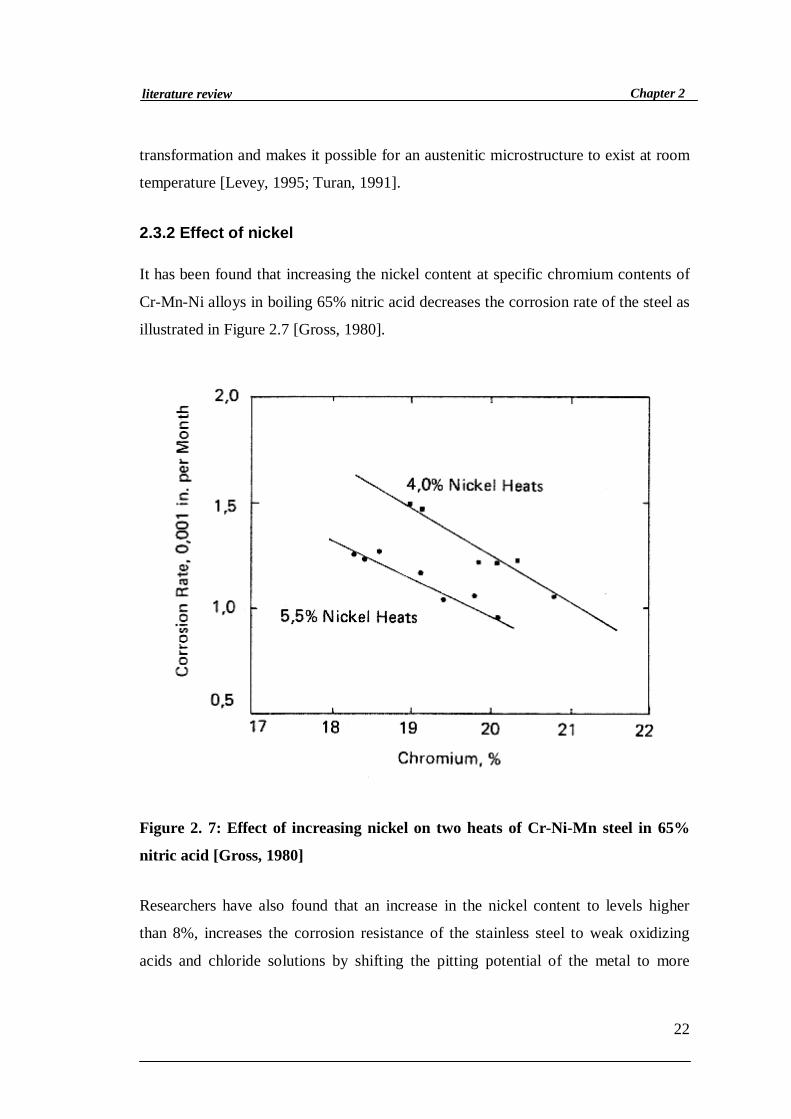
It has been found that increasing the nickel content at specific chromium contents of
Cr-Mn-Ni alloys in boiling 65% nitric acid decreases the corrosion rate of the steel as
illustrated in Figure 2.7 [Gross, 1980].
Figure 2. 7: Effect of increasing nickel on two heats of Cr-Ni-Mn steel in 65%
nitric acid [Gross, 1980]
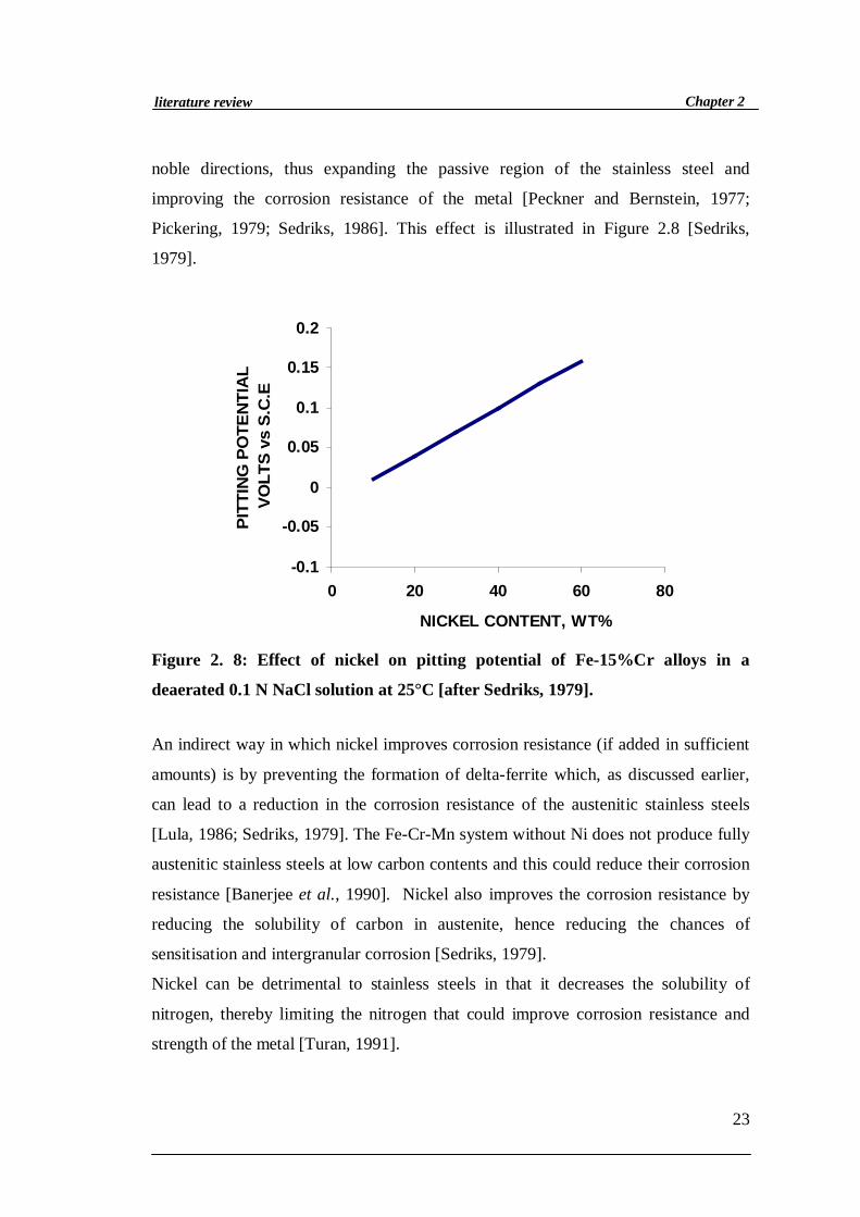
Researchers have also found that an increase in the nickel content to levels higher
than 8%, increases the corrosion resistance of the stainless steel to weak oxidizing
acids and chloride solutions by shifting the pitting potential of the metal to more
23
Chapter 2literature review
noble directions, thus expanding the passive region of the stainless steel and
improving the corrosion resistance of the metal [Peckner and Bernstein, 1977;
Pickering, 1979; Sedriks, 1986]. This effect is illustrated in Figure 2.8 [Sedriks,
1979].
-0.1
-0.05
0
0.05
0.1
0.15
0.2
0 20 40 60 80
NICKEL CONTENT, WT%
PITT
ING
PO
TEN
TIA
L V
OLT
S vs
S.C
.E
Figure 2. 8: Effect of nickel on pitting potential of Fe-15%Cr alloys in a
deaerated 0.1 N NaCl solution at 25°C [after Sedriks, 1979].
An indirect way in which nickel improves corrosion resistance (if added in sufficient
amounts) is by preventing the formation of delta-ferrite which, as discussed earlier,
can lead to a reduction in the corrosion resistance of the austenitic stainless steels
[Lula, 1986; Sedriks, 1979]. The Fe-Cr-Mn system without Ni does not produce fully
austenitic stainless steels at low carbon contents and this could reduce their corrosion
resistance [Banerjee et al., 1990]. Nickel also improves the corrosion resistance by
reducing the solubility of carbon in austenite, hence reducing the chances of
sensitisation and intergranular corrosion [Sedriks, 1979].
Nickel can be detrimental to stainless steels in that it decreases the solubility of
nitrogen, thereby limiting the nitrogen that could improve corrosion resistance and
strength of the metal [Turan, 1991].
24
Chapter 2literature review
2.3.3 Effect of manganese
Manganese is an austenite former that can be used to replace nickel since it has the
ability to extend the austenite loop and stabilize it at room temperature [Cortie, 1995;
Lula, 1986; Peckner and Bernstein, 1977; Wellbeloved 1990]. Manganese also has
the advantage of being less expensive than nickel. As a rule of thumb, when
replacing nickel with manganese in austenitic stainless steels, the ratio of Mn:Ni is
2:1 [Lula, 1986]; because manganese is a weaker austenite former than nickel and has
to be added in larger amounts to produce a fully austenitic microstructure [Gross and
Robinson, 1981].
Manganese aids nitrogen solubility and is almost always used in conjunction with this
element. Manganese in general is deemed to have a negative effect on the corrosion
resistance of stainless steel and has also been found to weaken the passive film,
increase ipass and thus decrease the protectiveness of the film [Gross and Robinson,
1981]. Figure 2.9 shows the negative effect of manganese on the corrosion resistance
of 17.5% Cr, 4% Ni steels in 65% nitric acid [Gross, 1980].
25
Chapter 2literature review
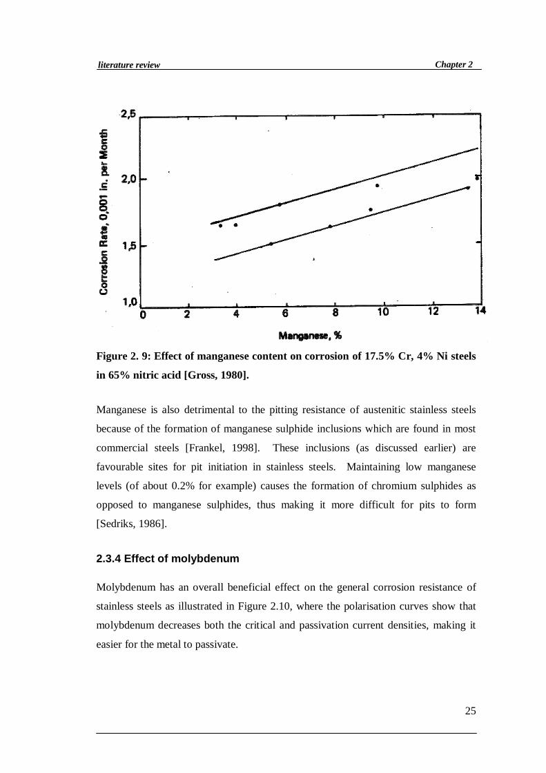
Figure 2. 9: Effect of manganese content on corrosion of 17.5% Cr, 4% Ni steels
in 65% nitric acid [Gross, 1980].
Manganese is also detrimental to the pitting resistance of austenitic stainless steels
because of the formation of manganese sulphide inclusions which are found in most
commercial steels [Frankel, 1998]. These inclusions (as discussed earlier) are
favourable sites for pit initiation in stainless steels. Maintaining low manganese
levels (of about 0.2% for example) causes the formation of chromium sulphides as
opposed to manganese sulphides, thus making it more difficult for pits to form
[Sedriks, 1986].
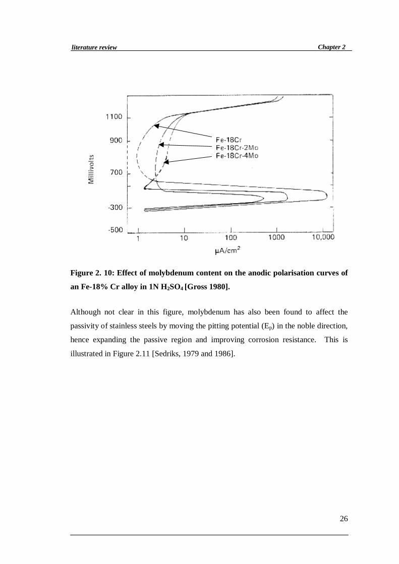
2.3.4 Effect of molybdenum
Molybdenum has an overall beneficial effect on the general corrosion resistance of
stainless steels as illustrated in Figure 2.10, where the polarisation curves show that
molybdenum decreases both the critical and passivation current densities, making it
easier for the metal to passivate.
26
Chapter 2literature review
Figure 2. 10: Effect of molybdenum content on the anodic polarisation curves of
an Fe-18% Cr alloy in 1N H2SO4 [Gross 1980].
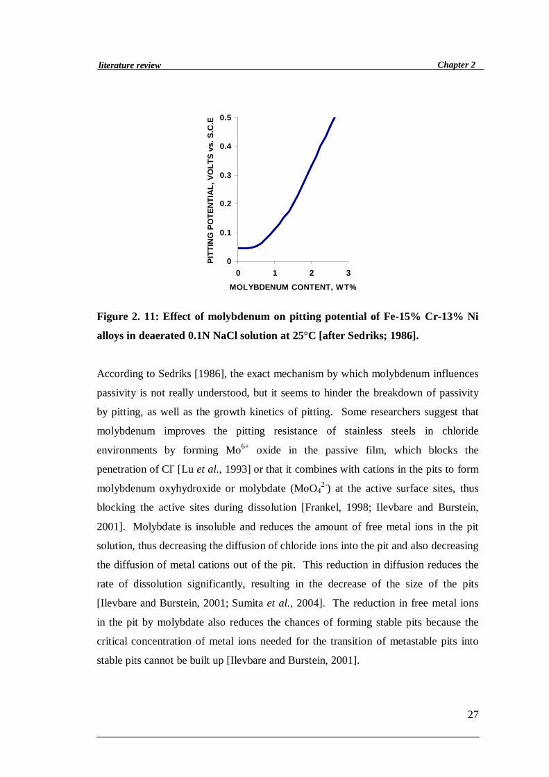
Although not clear in this figure, molybdenum has also been found to affect the
passivity of stainless steels by moving the pitting potential (Ep) in the noble direction,
hence expanding the passive region and improving corrosion resistance. This is
illustrated in Figure 2.11 [Sedriks, 1979 and 1986].
27
Chapter 2literature review
0
0.1
0.2
0.3
0.4
0.5
0 1 2 3
MOLYBDENUM CONTENT, WT%
PITT
ING
PO
TEN
TIA
L, V
OLT
S vs
. S.C
.E
Figure 2. 11: Effect of molybdenum on pitting potential of Fe-15% Cr-13% Ni
alloys in deaerated 0.1N NaCl solution at 25°C [after Sedriks; 1986].
According to Sedriks [1986], the exact mechanism by which molybdenum influences
passivity is not really understood, but it seems to hinder the breakdown of passivity
by pitting, as well as the growth kinetics of pitting. Some researchers suggest that
molybdenum improves the pitting resistance of stainless steels in chloride
environments by forming Mo6+ oxide in the passive film, which blocks the
penetration of Cl- [Lu et al., 1993] or that it combines with cations in the pits to form
molybdenum oxyhydroxide or molybdate (MoO42-) at the active surface sites, thus
blocking the active sites during dissolution [Frankel, 1998; Ilevbare and Burstein,
2001]. Molybdate is insoluble and reduces the amount of free metal ions in the pit
solution, thus decreasing the diffusion of chloride ions into the pit and also decreasing
the diffusion of metal cations out of the pit. This reduction in diffusion reduces the
rate of dissolution significantly, resulting in the decrease of the size of the pits
[Ilevbare and Burstein, 2001; Sumita et al., 2004]. The reduction in free metal ions
in the pit by molybdate also reduces the chances of forming stable pits because the
critical concentration of metal ions needed for the transition of metastable pits into
stable pits cannot be built up [Ilevbare and Burstein, 2001].

28
Chapter 2literature review
It has also been suggested that molybdenum improves passivity by promoting the
formation of Cr-O-OH (which has better protective properties that chromium oxide)
and hence improve the corrosion resistance of the steel [Lu et al., 1993].
In context of this project molybdenum has the disadvantage that it is a strong ferrite
former that needs to be balanced out with nickel and nitrogen and it is relatively
expensive [Schollenberger, 1995].
2.3.5 Effect of nitrogen
Since the nitrogen content of the atmosphere is 79%, N is present in all steel alloys,
as a result of atmospheric pick-up during manufacturing [Levey, 1995]. Stainless
steels, however, have a deliberately higher nitrogen content. Nitrogen is useful to
stainless steels not only because it is a strong austenite former and stabilizer, as is
evident from its high coefficient in equation 2.2, but also because it strengthens the
steel by means of solid solution strengthening. This occurs through nitrogen
decreasing the stacking fault energy and hence increasing the work hardening rate,
without unfavourably affecting the ductility and fracture toughness of the metal [Iorio
et al., 1994; Levey, 1995; Turan, 1991; Vismer 1997].
The beneficial effect of nitrogen on the corrosion resistance of austenitic stainless
steels has been attributed to it homogenising the microstructure by eliminating delta-
ferrite and stabilising the austeniteic microstructure [Jargelius-Pattersson, 1999].
It is important to consider nitrogen solubility when using it as an alloying element so
that unwanted ingot effects, such as porosity, and difficulties during hot working of
the metal can be avoided. Alloys made with nitrogen additions tend to form porosity
due to nitrogen coming out of solution during solidification [Iorio et al., 1994]. If the
solubility limit of nitrogen in the microstructure is exceeded then chromium nitride
29
Chapter 2literature review
precipitates will form in the matrix and these are detrimental to the corrosion
properties of the material because they form chromium-depleted zones in the matrix
which are susceptible to pitting attack [Levey, 1995]. To ensure the solid solubility
of nitrogen in chromium-containing austenite, nitrogen levels of 0.3% or above
require relatively high levels of manganese (e.g. 4%) [Sedriks, 1986]. This is because
manganese aids the solubility of nitrogen and a lower amount of manganese would
not be sufficient in providing good nitrogen solubility. In conventional austenitic
stainless steels, the solubility of nitrogen is about 0.2 wt% [Jargelius– Pattersson,
1994].
Factors that influence nitrogen solubility in iron alloys are composition, crystal
structure, temperature and the pressure of gaseous nitrogen in the atmosphere above
the alloy [Iorio et al., 1994]. Elements such as nickel, carbon, silicon and copper
decrease nitrogen solubility while chromium, manganese and molybdenum increase it
[Iorio et al., 1994; Levey, 1995; Vismer, 1997].
There is much debate as to the effect of nitrogen on the general corrosion resistance
of stainless steels in acids [Levey, 1995]. Nitrogen has been found to have an adverse
effect on the corrosion resistance of stainless steels in different acid mediums [Levey,
1995] but it has also been found to improve the corrosion resistance of molybdenum-
free austenitic stainless steel. The addition of nitrogen to the molybdenum free-
steels, has been found to be beneficial to the development of passivity in sulphuric
acid as is illustrated in Figure 2.12 [Gross 1980], since an increase of nitrogen in
austenitic stainless steels decreased ipass and icrit, making passivation easier.
30
Chapter 2literature review
Figure 2. 12: Anodic polarisation curves for 18% Cr-8% Ni SSs containing
various amounts of nitrogen, tested in a hydrogen-purged 1N H2SO4 + 0.5 M
NaCl solution at ambient temperature [Gross 1980].
There seems, however, to be an agreement that nitrogen improves the general
corrosion resistance of duplex and martensitic stainless steels more significantly than
of the austenitic stainless steels. Nitrogen additions to austenitic stainless steels have
a small to moderate effect on improving their general corrosion resistance. Ferritic
stainless steels have a low solubility for nitrogen, so the addition of nitrogen is
detrimental to the corrosion resistance of these steels.
When considering pitting corrosion however, small additions of nitrogen improve the
pitting resistance of austenitic stainless steels, provided the solubility limit is not
exceeded [Brigham and Tozer, 1974; Frankel, 1998; Levey, 1995,; Rondelli et al.,
1995; Sedriks 1983] as shown in Figure 2.13:
31
Chapter 2literature review
0
200
400
600
800
1000
0 0.1 0.2 0.3 0.4 0.5
NITROGEN CONTENT OF STEEL, wt-%
PITT
ING
PO
TEN
TIA
L, m
V (S
CE)
specimen with creviceplain specimen
Figure 2. 13: Effect of Nitrogen content on pitting potential of 22Cr-20Ni-4Mn-
2.8Mo-0.03C-0.01S stainless steel in aerated aqueous solution containing 0.6 M
NaCl and 0.1 M NaHCO3 [after Sedriks 1983].
The beneficial effect of nitrogen in improving pitting resistance can also be seen by
its high coefficient in the PRE equation (equation 2.7).
There are many opinions offered to explain how nitrogen improves the localised
corrosion of stainless steels. One suggestion is that nitrogen in solid solution
dissolves to form ammonium ions (NH4+) according to equation 2.8 [Baba et al.,
2002; Jargelius-Patterson, 1999]:
+−+ →++ 434 NHeHN Equation 2. 8

32
Chapter 2literature review
These ammonium ions consume protons during pit initiation, thus increasing the pH
and helping to passivate the pit before it can become a stable growing pit [Jargelius-
Patterson, 1999; Levey 1995]. These ammonium ions could further hydrolyse to
form species such as NO2- or NO3
- which are inhibitors of corrosion. Inhibitors can
stifle the action of the chloride ion as a pitting agent [Shams et al., 1999].
Ammonium ions could also combine with active oxidants such as free chlorine and
bromine to form chloramines or bromo-amines which are less active products and
therefore are less aggressive to the metal [Jargelius-Patterson, 1999].
Investigators have also suggested that nitrogen concentrates at the passive film/metal
interface to stabilise the film and prevent attack of anions such as chlorides. This
nitrogen is suggested to aid the repassivation of the film and increase the pitting
corrosion resistance of the film [Baba et al., 2002].
Nitrogen further improves pitting resistance of stainless steels by expanding the
passive region of the metal through the shifting of the pitting potential (Ep) in a
nobler direction [Sedriks, 1986]. This effect is more beneficial in stainless steels
containing molybdenum because the Ep is shifted even further in the noble direction
when molybdenum is present, thus providing maximum expansion of the passive
region of the metal [Sedriks, 1986].
The synergistic effect of nitrogen and molybdenum in improving pitting and general
corrosion resistance of stainless steel is a significant factor to consider. For example,
once the molybdenum has shifted the pitting potential to higher values than normal
and if sufficiently high potentials are reached, nitrogen can then accumulate at active
dissolution sites, blocking them from the harsh environment [Jargelius-Patterson,
1999]. It has also been suggested that molybdenum and nitrogen interact to form a
protective layer on the surface of the steel. Nitrogen is thought to promote the
formation of molybdenum nitrides which inhibit the dissolution of molybdenum in
the transpassive region, retaining the molybdenum in the passive film [Jargelius-
33
Chapter 2literature review
Patterson, 1999]. Nitrogen may also form ammonia ligands which raise the local pH,
thus promoting the formation of molybdate, which assists in the formation of
ammonium, further improving the passivity of the stainless steel [Jargelius-Patterson,
1999].
Improvement in grain boundary corrosion resistance has also been attributed to
nitrogen additions, because when sensitisation temperatures are reached, the nitrogen
can diffuse faster than the carbon to the grain boundaries so that chromium nitride
(Cr2N), rather than chromium carbide (Cr23C6), precipitates are formed [Turan, 1991].
Although the area around the grain boundaries is depleted of chromium, the depletion
is not as severe as when chromium carbide precipitates are formed.
In conclusion, alloying elements have important effects on the corrosion behaviour of
stainless steels: Figure 2.14 is an overall summary of their effects [Sedriks, 1986]
34
Chapter 2literature review
Figure 2. 14: Schematic summary of the effect of alloying elements in stainless
steels on the anodic polarization curve [after Sedriks, 1986]
Chromium, molybdenum, nitrogen and nickel are beneficial to the corrosion
resistance of stainless steels since they improve passivity by decreasing the critical
current density and the passivation current. Manganese has been found to be
detrimental to the corrosion resistance of stainless steels.
2.4 Effect of microstructure and processing on the corrosion
behaviour of stainless steels
Microstructure is affected by alloying elements, which in turn affects the corrosion
resistance of the stainless steels. Other factors that play a part in determining the
microstructure are the processes and methods used to produce and treat the material.
Castings have inhomogenous structures, rolling and extrusion methods can cause the
material to have texture, while elongated grains, hot working and annealing can

35
Chapter 2literature review
produce anisotropy in the microstructure. All these factors will affect the corrosion
behaviour of the material [Simpson, 1990]. Cold worked or plastically deformed
parts of a metal are more susceptible to corrosion than if the metal was annealed
[Callister, 1994]. This is because the worked part of a material stores a great deal of
energy, making it more active or anodic compared to the rest of the material. Delta-
ferrite and manganese sulphide inclusions, as already mentioned, decrease corrosion
resistance. In fact, any irregularity or inclusion in the microstructure can provide a
site for pit nucleation.
The pitting potential of stainless steels in chloride solutions has been found to depend
highly on the degree of cold work and the orientation of the sample [Simpson, 1990].
It has been found that the pitting potential decreases with cold work and that it is
higher in the longitudinal than transverse direction. It has also been concluded from
experiments done on austenitic stainless steels in acid solutions that passivation in the
longitudinal direction is ten times easier than that in the transverse direction at 30%
cold work [Simpson, 1990].
From the literature survey it is evident that there are a number of factors that can
simultaneously affect the corrosion resistance of stainless steel. Stainless steels can
suffer both general and pitting corrosion depending on the nature of the steel and the
environment. Researchers have found molybdenum and nitrogen to improve the
general corrosion resistance of austenitic stainless steels, but not as effectively as they
improve the pitting corrosion resistance. Manganese increases nitrogen solubilty of
stainless steels but it forms manganese sulphides which are detrimental to the
corrosion resistance of stainless steels. The correct balance of the alloys however can
produce a steel that has good mechanical and corrosion resistance. Alloying elements
can thus act individually or synergistically in determining the corrosion behaviour of
stainless steels.
36
Chapter 2literature review
The alloys that were investigated in this project were all based on the Hercules
alloy with variations in manganese, molybdenum and nitrogen. The aim was to find a
combination of these alloys so that a more corrosion resistant version of the currently
existing Hercules can be found. The original Hercules has no molybdenum
additions and it is assumed that the addition of molybdenum could improve the
corrosion resistance of this alloy. This is all discussed in the next chapters.

37
Chapter 3
3. Production of the alloys
A matrix of eighteen alloys were designed to systematically analyse the effect of
varying levels of Mn, N and Mo on the corrosion behaviour of the Hercules steel.
Firstly, trial melts of 50g buttons were made to establish the alloying practice and
allow for initial corrosion testing. This gave valuable information that enabled the
successful production of 5kg ingots. The melting and production practice, targeted
and actual chemical composition, as well as microstructures of these alloys are
discussed in this chapter.
3.1 General
The alloys that were made for this investigation were targeted at a Hercules base
composition of 0.04 wt% C, 16 wt% Cr, 2 wt% Ni, 0.5 wt% Si, and 0.01 wt% P. Mn,
N and Mo were varied in two or three levels, as listed in table 3.1 to produce eighteen
test alloys.
38
Chapter 3production of alloys
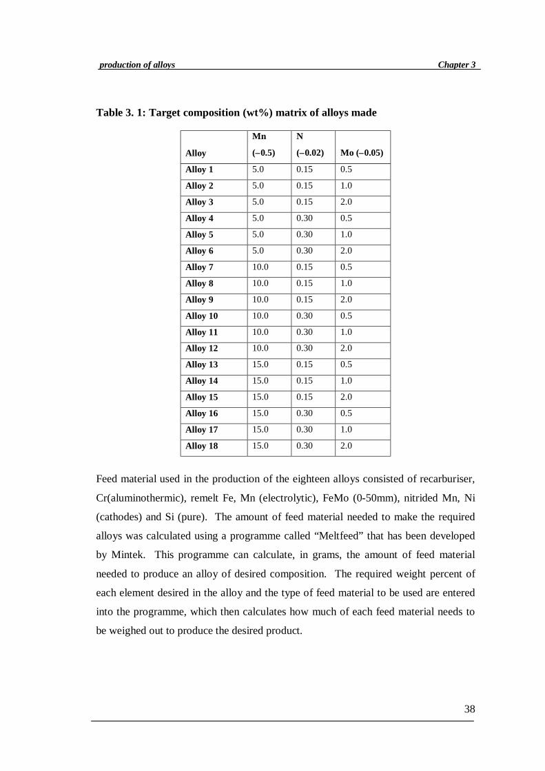
Table 3. 1: Target composition (wt%) matrix of alloys made
Alloy
Mn
(±0.5)
N
(±0.02) Mo (±0.05)
Alloy 1 5.0 0.15 0.5
Alloy 2 5.0 0.15 1.0
Alloy 3 5.0 0.15 2.0
Alloy 4 5.0 0.30 0.5
Alloy 5 5.0 0.30 1.0
Alloy 6 5.0 0.30 2.0
Alloy 7 10.0 0.15 0.5
Alloy 8 10.0 0.15 1.0
Alloy 9 10.0 0.15 2.0
Alloy 10 10.0 0.30 0.5
Alloy 11 10.0 0.30 1.0
Alloy 12 10.0 0.30 2.0
Alloy 13 15.0 0.15 0.5
Alloy 14 15.0 0.15 1.0
Alloy 15 15.0 0.15 2.0
Alloy 16 15.0 0.30 0.5
Alloy 17 15.0 0.30 1.0
Alloy 18 15.0 0.30 2.0
Feed material used in the production of the eighteen alloys consisted of recarburiser,
Cr(aluminothermic), remelt Fe, Mn (electrolytic), FeMo (0-50mm), nitrided Mn, Ni
(cathodes) and Si (pure). The amount of feed material needed to make the required
alloys was calculated using a programme called “Meltfeed” that has been developed
by Mintek. This programme can calculate, in grams, the amount of feed material
needed to produce an alloy of desired composition. The required weight percent of
each element desired in the alloy and the type of feed material to be used are entered
into the programme, which then calculates how much of each feed material needs to
be weighed out to produce the desired product.
39
Chapter 3production of alloys
Inevitably, there are some losses during the making of alloys, especially with regard
to C, Mn and N, and extra feed material is added to compensate for these losses.
Knowledge of the amount of extra feed material to add is based on experience.
According to K.P Mokaleng of Mintek, an extra 10% C and Mn and an extra 15% N
is usually added to compensate for losses. The eighteen alloys were thus
manufactured with the above mentioned extra feed material.
3.2 Melting procedure
When making alloys, inclusions and impurities are a major concern, since they can
affect corrosion results. Great care was thus placed in melting the alloys. The 50g
buttons and 5kg ingots were both melted in an argon atmosphere and the procedures
followed to melt these alloys are discussed in this section.
3.2.1 The 50g buttons
The 50g buttons were made in a button arc furnace in an argon atmosphere. The
furnace was first flushed with argon three times to remove oxygen before filling it
with Ar. Pure Ti was melted in the button arc furnace prior to melting the feed
material to ensure the removal of any residual oxygen. The heavier feed materials
were melted first, while the lighter recarburiser and nitrided manganese were melted
last. This was done to ensure that the light material did not blow away during
melting. Once the feed material was melted into a button, the button was remelted
two more times to ensure homogeneity. The button was then left to cool in the
furnace.
The eighteen buttons were approximately 30 mm in diameter and were homogenised
at 1200ºC for four hours and quenched. The buttons were then sand blasted to
remove some of the oxide layer and, using a Feritscope ® MP30 ferritescope, the
magnetic content of the buttons was measured. The buttons were manufactured with
40
Chapter 3production of alloys
the intent of them having an austenitic microstructure. Austenite is not magnetic,
thus a ferritescope reading of 0 would be ideal. It was noted, however, in previous
experiments [Kerr, 2003] that a ferritescope reading of less than 10 usually meant that
the alloy was austenitic. The magnetic readings of all eighteen buttons were taken on
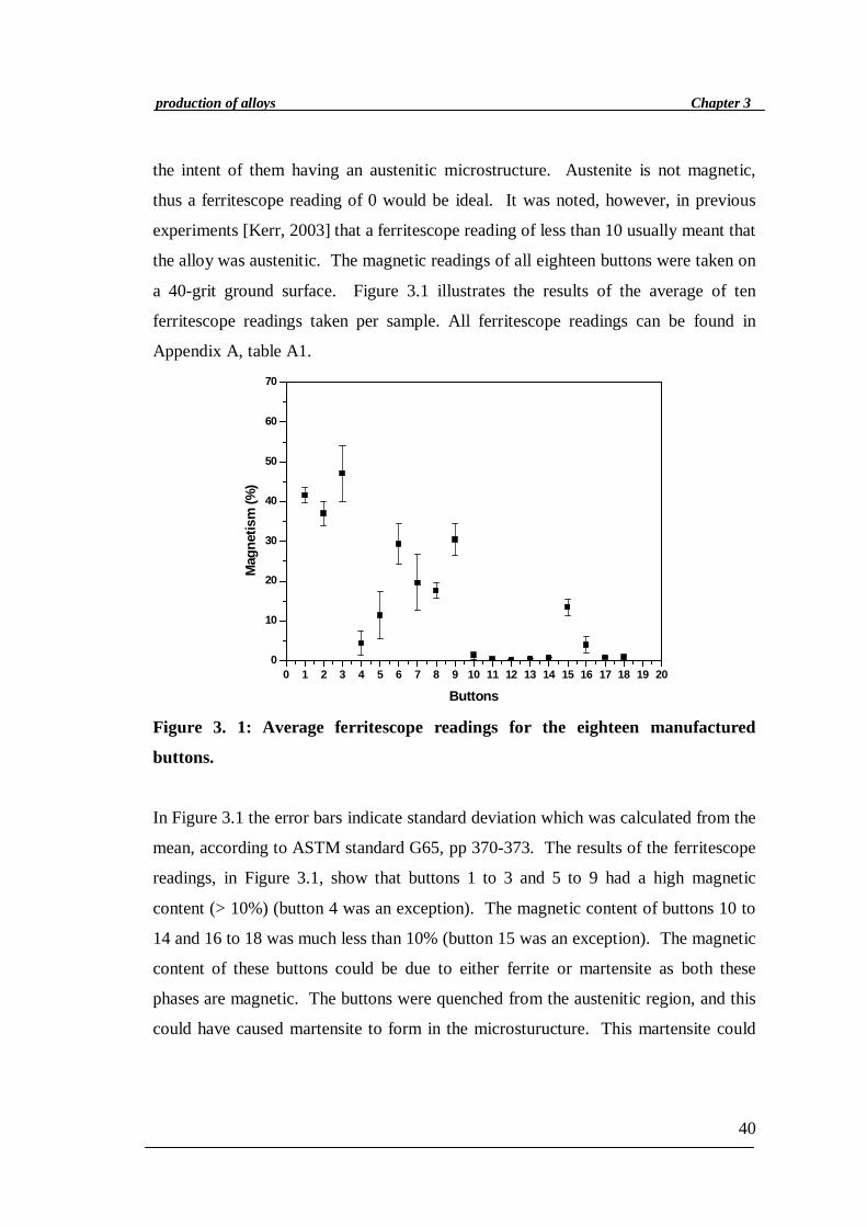
a 40-grit ground surface. Figure 3.1 illustrates the results of the average of ten
ferritescope readings taken per sample. All ferritescope readings can be found in
Appendix A, table A1.
0 1 2 3 4 5 6 7 8 9 10 11 12 13 14 15 16 17 18 19 200
10
20
30
40
50
60
70
Mag
netis
m (%
)
Buttons
Figure 3. 1: Average ferritescope readings for the eighteen manufactured
buttons.
In Figure 3.1 the error bars indicate standard deviation which was calculated from the
mean, according to ASTM standard G65, pp 370-373. The results of the ferritescope
readings, in Figure 3.1, show that buttons 1 to 3 and 5 to 9 had a high magnetic
content (> 10%) (button 4 was an exception). The magnetic content of buttons 10 to
14 and 16 to 18 was much less than 10% (button 15 was an exception). The magnetic
content of these buttons could be due to either ferrite or martensite as both these
phases are magnetic. The buttons were quenched from the austenitic region, and this
could have caused martensite to form in the microsturucture. This martensite could
41
Chapter 3production of alloys
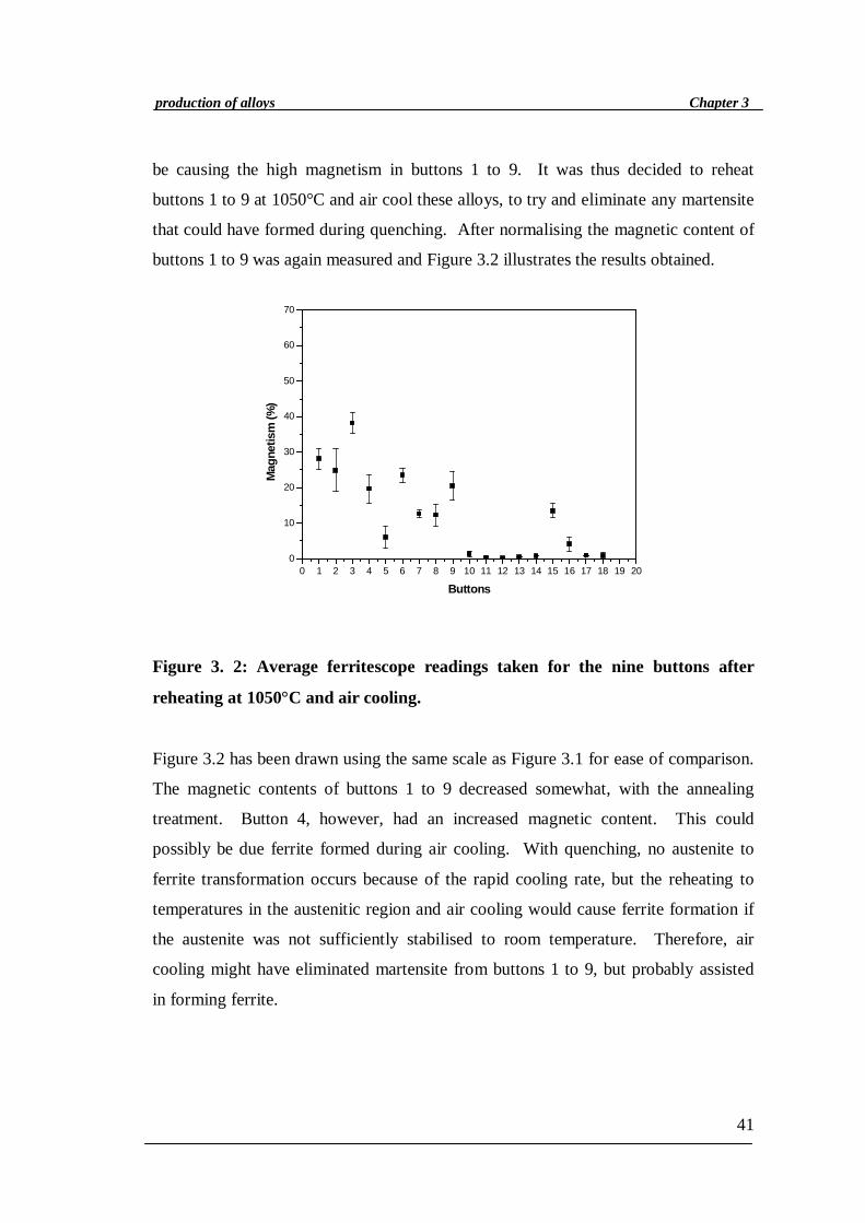
be causing the high magnetism in buttons 1 to 9. It was thus decided to reheat
buttons 1 to 9 at 1050°C and air cool these alloys, to try and eliminate any martensite
that could have formed during quenching. After normalising the magnetic content of
buttons 1 to 9 was again measured and Figure 3.2 illustrates the results obtained.
0 1 2 3 4 5 6 7 8 9 10 11 12 13 14 15 16 17 18 19 200
10
20
30
40
50
60
70
Mag
netis
m (%
)
Buttons
Figure 3. 2: Average ferritescope readings taken for the nine buttons after
reheating at 1050°C and air cooling.
Figure 3.2 has been drawn using the same scale as Figure 3.1 for ease of comparison.
The magnetic contents of buttons 1 to 9 decreased somewhat, with the annealing
treatment. Button 4, however, had an increased magnetic content. This could
possibly be due ferrite formed during air cooling. With quenching, no austenite to
ferrite transformation occurs because of the rapid cooling rate, but the reheating to
temperatures in the austenitic region and air cooling would cause ferrite formation if
the austenite was not sufficiently stabilised to room temperature. Therefore, air
cooling might have eliminated martensite from buttons 1 to 9, but probably assisted
in forming ferrite.
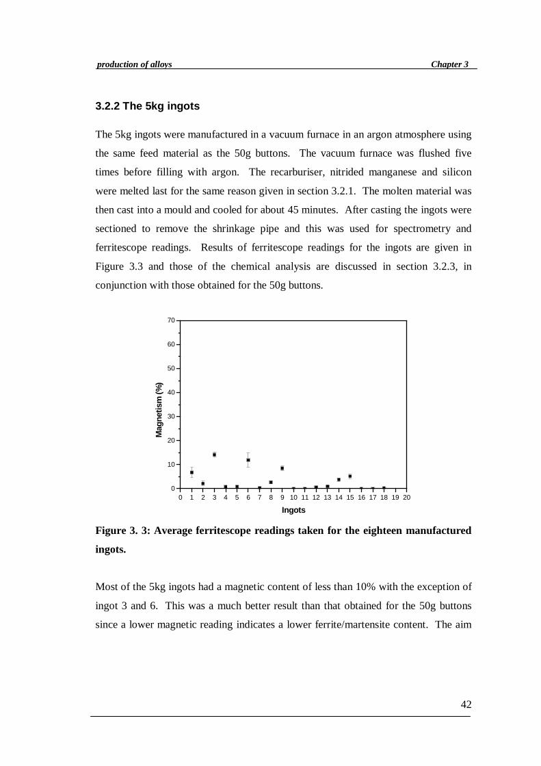
42
Chapter 3production of alloys
3.2.2 The 5kg ingots
The 5kg ingots were manufactured in a vacuum furnace in an argon atmosphere using
the same feed material as the 50g buttons. The vacuum furnace was flushed five
times before filling with argon. The recarburiser, nitrided manganese and silicon
were melted last for the same reason given in section 3.2.1. The molten material was
then cast into a mould and cooled for about 45 minutes. After casting the ingots were
sectioned to remove the shrinkage pipe and this was used for spectrometry and
ferritescope readings. Results of ferritescope readings for the ingots are given in
Figure 3.3 and those of the chemical analysis are discussed in section 3.2.3, in
conjunction with those obtained for the 50g buttons.
0 1 2 3 4 5 6 7 8 9 10 11 12 13 14 15 16 17 18 19 200
10
20
30
40
50
60
70
Mag
netis
m (%
)
Ingots
Figure 3. 3: Average ferritescope readings taken for the eighteen manufactured
ingots.
Most of the 5kg ingots had a magnetic content of less than 10% with the exception of
ingot 3 and 6. This was a much better result than that obtained for the 50g buttons
since a lower magnetic reading indicates a lower ferrite/martensite content. The aim
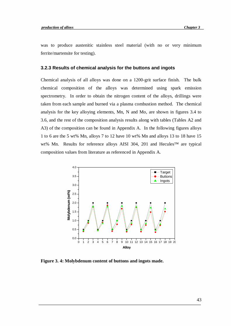
43
Chapter 3production of alloys
was to produce austenitic stainless steel material (with no or very minimum
ferrite/martensite for testing).
3.2.3 Results of chemical analysis for the buttons and ingots
Chemical analysis of all alloys was done on a 1200-grit surface finish. The bulk
chemical composition of the alloys was determined using spark emission
spectrometry. In order to obtain the nitrogen content of the alloys, drillings were
taken from each sample and burned via a plasma combustion method. The chemical
analysis for the key alloying elements, Mn, N and Mo, are shown in figures 3.4 to
3.6, and the rest of the composition analysis results along with tables (Tables A2 and
A3) of the composition can be found in Appendix A. In the following figures alloys
1 to 6 are the 5 wt% Mn, alloys 7 to 12 have 10 wt% Mn and alloys 13 to 18 have 15
wt% Mn. Results for reference alloys AISI 304, 201 and Hecules™ are typical
composition values from literature as referenced in Appendix A.
0 1 2 3 4 5 6 7 8 9 10 11 12 13 14 15 16 17 18 19 200.0
0.5
1.0
1.5
2.0
2.5
3.0
3.5
4.0
Mol
ybde
num
(wt%
)
Alloy
Target Buttons Ingots
Figure 3. 4: Molybdenum content of buttons and ingots made.

44
Chapter 3production of alloys
0 1 2 3 4 5 6 7 8 9 10 11 12 13 14 15 16 17 18 19 200
2
4
6
8
10
12
14
16
18
20
22
24
Herc
201
304
Man
gane
se (w
t%)
Alloy
target buttons ingots
Figure 3. 5: Manganese content of buttons and ingots made.
The actual Mo and Mn contents of the alloys (figures 3.4 and 3.5) were generally
close to target and in the instances where they deviated from target the difference was
small. No reference values are shown in Figure 3.5 since reference alloys typically
have no molybdenum content. One significant deviation to note though was the Mn
content of alloy 13 for the 50g buttons, which was much lower than expected. The C,
Ni and Cr contents in Appendix A (Figures A1 to A3) were also within the target
range. The N content of the alloys, however, deviated significantly from target, as
illustrated in Figure 3.6.

45
Chapter 3production of alloys
0 1 2 3 4 5 6 7 8 9 10 11 12 13 14 15 16 17 18 19 200.0
0.1
0.2
0.3
0.4
0.5
0.6
0.7
Herc
201
30415 wt% Mn10 wt% Mn5 wt% Mn
Nitr
ogen
(wt%
)
Alloy
target buttons ingots
Figure 3. 6: Nitrogen content of buttons and ingots made.
Referring to the actual nitrogen content of the 50g buttons in Figure 3.6, the N
content seems to increase above target from button 11 to 18. These buttons all have
Mn contents of 10 wt% and more. An increase in Mn content increases the N
solubility in stainless steel and this could be the reason for the high N contents of
buttons 11 to 18. It was not possible though to get high N contents of 0.3 wt% for the
5 wt% Mn buttons 1 to 6. It was also not possible to attain high N contents for the
5kg ingots. The N content for the ingots was either on or below target, never above.
Figure 3.7 is a diagram showing the solubility of N as a function of both Mn and Cr
content at 1600°C and 0.80 atm N2 partial pressure [Kerr, 2003]. This diagram shows
the maximum solubility of N for a given Mn/Cr combination, and can be used to
explain why in some instances the N level was above or below target.
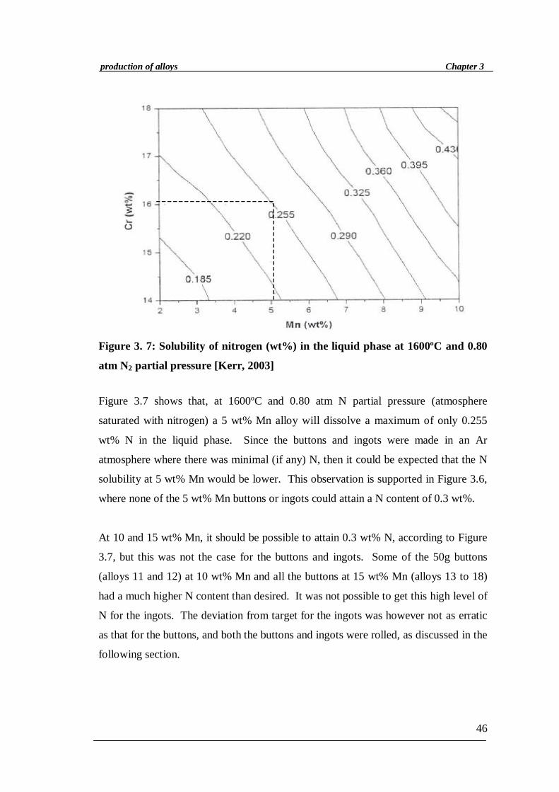
46
Chapter 3production of alloys
Figure 3. 7: Solubility of nitrogen (wt%) in the liquid phase at 1600ºC and 0.80
atm N2 partial pressure [Kerr, 2003]
Figure 3.7 shows that, at 1600ºC and 0.80 atm N partial pressure (atmosphere
saturated with nitrogen) a 5 wt% Mn alloy will dissolve a maximum of only 0.255
wt% N in the liquid phase. Since the buttons and ingots were made in an Ar
atmosphere where there was minimal (if any) N, then it could be expected that the N
solubility at 5 wt% Mn would be lower. This observation is supported in Figure 3.6,
where none of the 5 wt% Mn buttons or ingots could attain a N content of 0.3 wt%.
At 10 and 15 wt% Mn, it should be possible to attain 0.3 wt% N, according to Figure
3.7, but this was not the case for the buttons and ingots. Some of the 50g buttons
(alloys 11 and 12) at 10 wt% Mn and all the buttons at 15 wt% Mn (alloys 13 to 18)
had a much higher N content than desired. It was not possible to get this high level of
N for the ingots. The deviation from target for the ingots was however not as erratic
as that for the buttons, and both the buttons and ingots were rolled, as discussed in the
following section.

47
Chapter 3production of alloys
3.2.4 Rolling and heat treatment
3.2.4.1 The 50g buttons
The 50g buttons were rolled to a thickness of approximately 4.5 mm (± 55%
reduction). Buttons 1 to 9 (which had the highest magnetic content) were difficult to
roll because they work hardened easily and cracked after a few passes while buttons
10 to 18 rolled easier and showed only slight cracking. The rolling history of all the
alloys is shown in Table B1 of Appendix B. The ferritescope readings (magnetism
(%) also shown in the table) of the buttons increased during rolling, suggesting that
the alloys have metastable austenite which transforms to martensite upon cold rolling
at temperatures below the M(d30)3 temperature. This is to be expected since it was
found in literature that manganese steels have a high work hardening rate [Harvey,
1982; Levey 1985]. After rolling the alloys were annealed at 1100°C and air cooled
to eliminate the effects of cold rolling.
3.2.4.2 The 5kg ingots
After chemical analysis, the 5kg ingots were soaked at 1200°C for four hours for
homogenisation. Following that, the ingots were hot rolled according to the
following rolling sequence:
37-35-33 mmà reheat for 5 min at 1050°C à30-28-26 mm à reheat for 5 min at
1050°C à 23-21-19 mm à water quench.
After quenching the alloys were annealed at 1100°C for 2 hours and air cooled so that
any segregation or tension that was built up during quenching could be eliminated.
3 Md(30) =413 - 462(C+N) - 9.2Si -8.1Mn - 13.7Cr - 9.5Ni - 18.5Mo - 18.5Cu - 3Co [Angel, 1954;Paton et al, 2004]
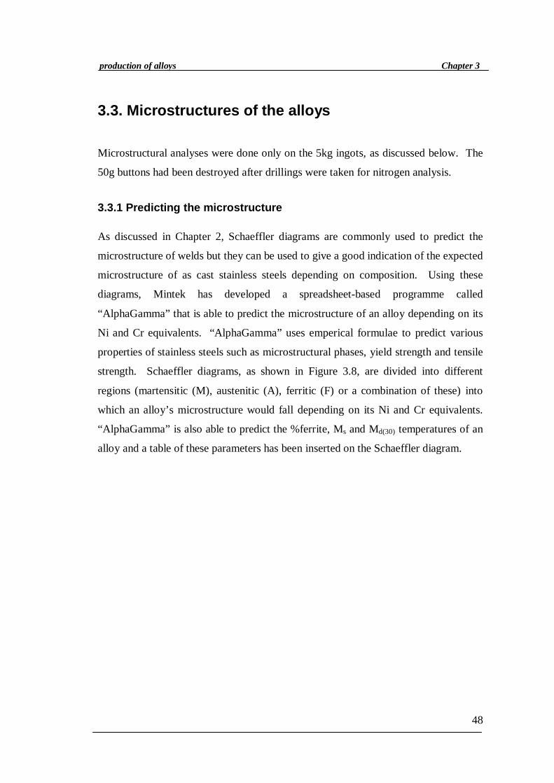
48
Chapter 3production of alloys
3.3. Microstructures of the alloys
Microstructural analyses were done only on the 5kg ingots, as discussed below. The
50g buttons had been destroyed after drillings were taken for nitrogen analysis.
3.3.1 Predicting the microstructure
As discussed in Chapter 2, Schaeffler diagrams are commonly used to predict the
microstructure of welds but they can be used to give a good indication of the expected
microstructure of as cast stainless steels depending on composition. Using these
diagrams, Mintek has developed a spreadsheet-based programme called
“AlphaGamma” that is able to predict the microstructure of an alloy depending on its
Ni and Cr equivalents. “AlphaGamma” uses emperical formulae to predict various
properties of stainless steels such as microstructural phases, yield strength and tensile
strength. Schaeffler diagrams, as shown in Figure 3.8, are divided into different
regions (martensitic (M), austenitic (A), ferritic (F) or a combination of these) into
which an alloy’s microstructure would fall depending on its Ni and Cr equivalents.
“AlphaGamma” is also able to predict the %ferrite, Ms and Md(30) temperatures of an
alloy and a table of these parameters has been inserted on the Schaeffler diagram.
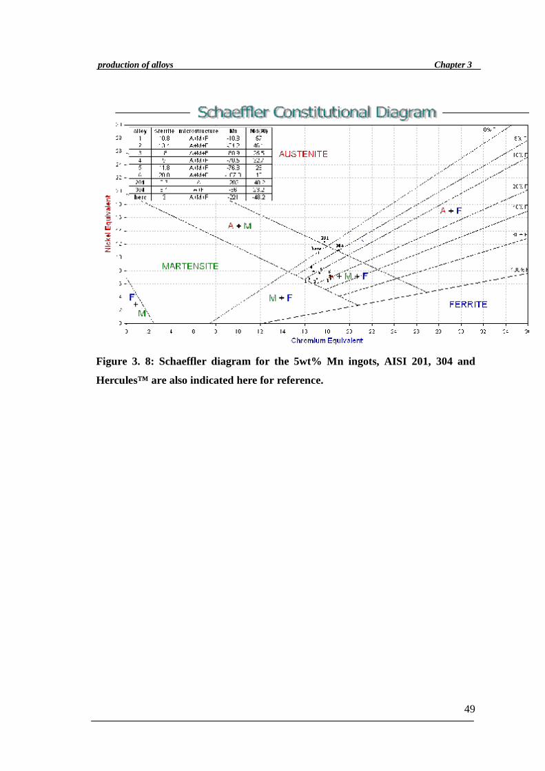
49
Chapter 3production of alloys
Figure 3. 8: Schaeffler diagram for the 5wt% Mn ingots, AISI 201, 304 and
Hercules™ are also indicated here for reference.
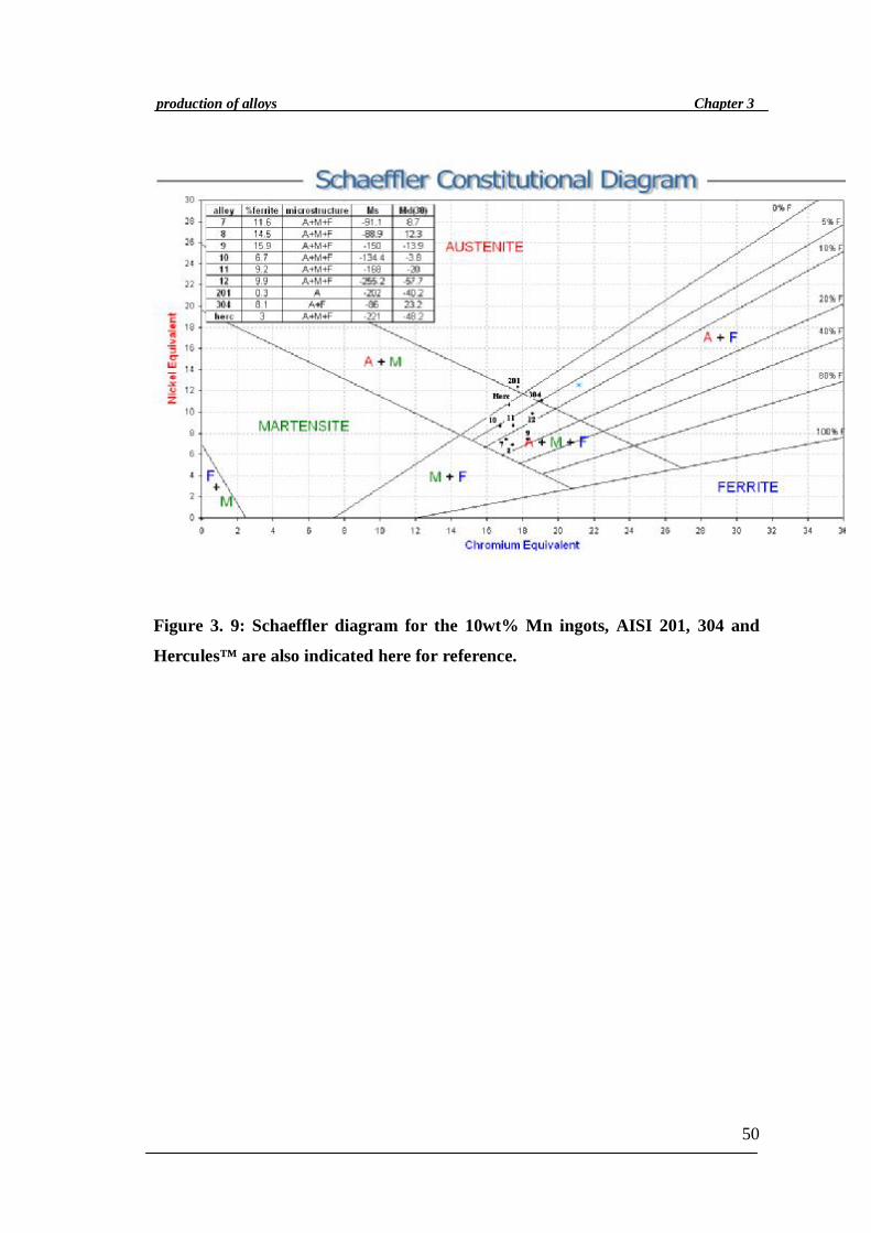
50
Chapter 3production of alloys
Figure 3. 9: Schaeffler diagram for the 10wt% Mn ingots, AISI 201, 304 and
Hercules™ are also indicated here for reference.
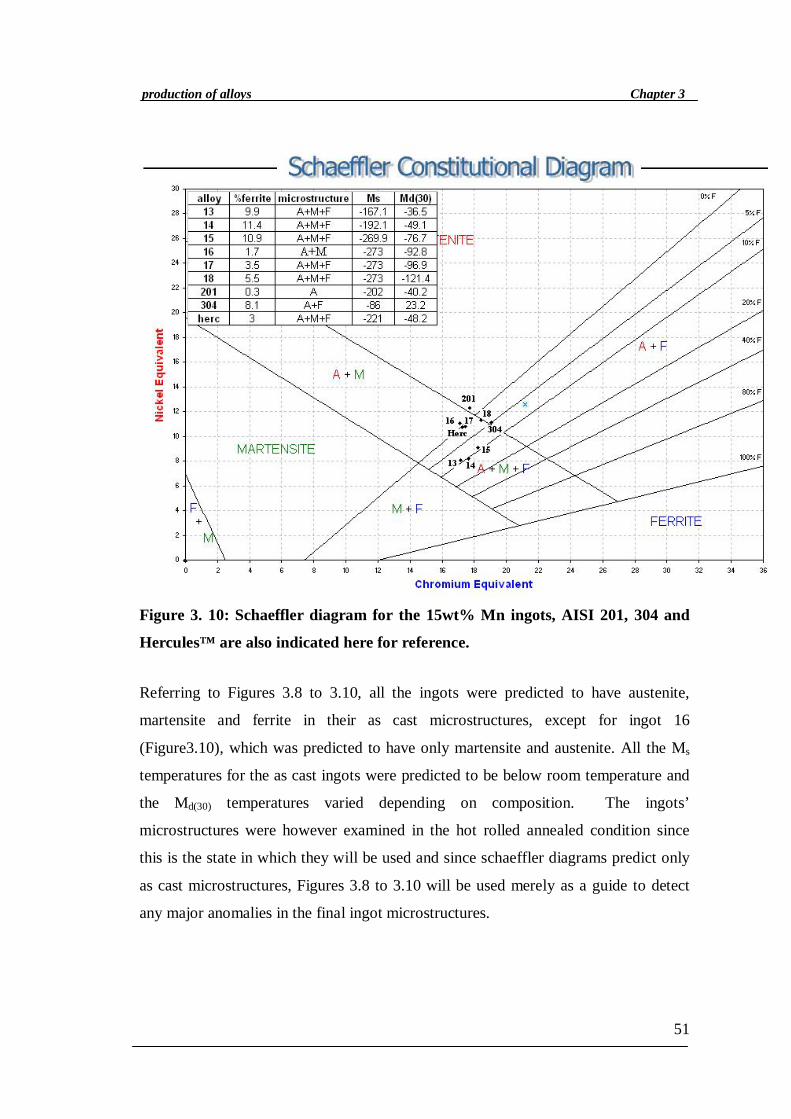
51
Chapter 3production of alloys
Figure 3. 10: Schaeffler diagram for the 15wt% Mn ingots, AISI 201, 304 and
Hercules™ are also indicated here for reference.
Referring to Figures 3.8 to 3.10, all the ingots were predicted to have austenite,
martensite and ferrite in their as cast microstructures, except for ingot 16
(Figure3.10), which was predicted to have only martensite and austenite. All the Ms
temperatures for the as cast ingots were predicted to be below room temperature and
the Md(30) temperatures varied depending on composition. The ingots’
microstructures were however examined in the hot rolled annealed condition since
this is the state in which they will be used and since schaeffler diagrams predict only
as cast microstructures, Figures 3.8 to 3.10 will be used merely as a guide to detect
any major anomalies in the final ingot microstructures.

52
Chapter 3production of alloys
3.4 Actual microstructure
3.4.1 Optical microscopy
From the 5kg ingots, material was cut transverse to the hot rolling direction, mounted
and etched to reveal the microstructure. Two etchants were used: 10% oxalic acid
and 75% potassium hydroxide (KOH). Both etchants were used to electro-etch the
alloys according to the parameters listed in Table 3.2.
Table 3. 2: Etchants used for electro-etching
Etchant 10% Oxalic acid 75% KOH
Contents 10g oxalic acid, 100 ml water 45g KOH, 60 ml water
Structure itreveals
General structure. Attacks austenite particularly
well but not delta-ferrite or martensite
Reveals delta-ferrite as dark brown and reveals austenite
as a light phase. Can also reveal martensite
Example ofstructure
revealed
Voltage 2.5 V 6 V
Time 2-6 sec 90 sec
The full set of microstructures of the alloys are given in Appendix C. From the
microstructural analysis it was found that all the ingots were mostly austenitic with
some ferrite, except for alloy 1 which had some lathe martensite. Hot rolling and
annealing would have altered the phase distributions as predicted by the schaeffler
diagrams, but since no microstructural analysis was done on the as cast sample this
could not be verified.
γ
Inclusion
α
γ
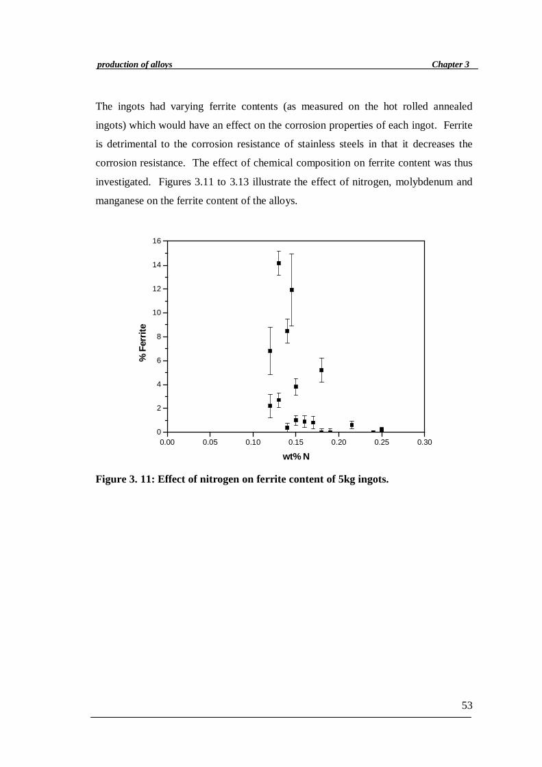
53
Chapter 3production of alloys
The ingots had varying ferrite contents (as measured on the hot rolled annealed
ingots) which would have an effect on the corrosion properties of each ingot. Ferrite
is detrimental to the corrosion resistance of stainless steels in that it decreases the
corrosion resistance. The effect of chemical composition on ferrite content was thus
investigated. Figures 3.11 to 3.13 illustrate the effect of nitrogen, molybdenum and
manganese on the ferrite content of the alloys.
0.00 0.05 0.10 0.15 0.20 0.25 0.300
2
4
6
8
10
12
14
16
% F
errit
e
wt% N
Figure 3. 11: Effect of nitrogen on ferrite content of 5kg ingots.
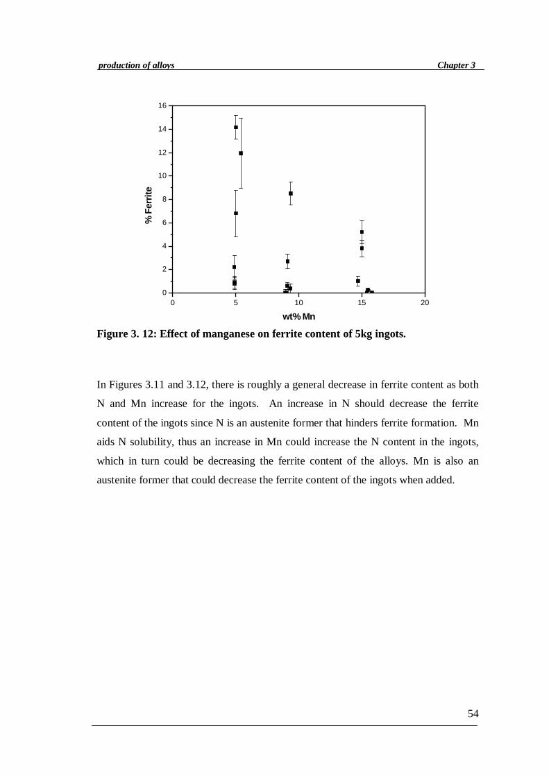
54
Chapter 3production of alloys
0 5 10 15 200
2
4
6
8
10
12
14
16
% F
errit
e
wt% Mn
Figure 3. 12: Effect of manganese on ferrite content of 5kg ingots.
In Figures 3.11 and 3.12, there is roughly a general decrease in ferrite content as both
N and Mn increase for the ingots. An increase in N should decrease the ferrite
content of the ingots since N is an austenite former that hinders ferrite formation. Mn
aids N solubility, thus an increase in Mn could increase the N content in the ingots,
which in turn could be decreasing the ferrite content of the alloys. Mn is also an
austenite former that could decrease the ferrite content of the ingots when added.

55
Chapter 3production of alloys
0.0 0.2 0.4 0.6 0.8 1.0 1.2 1.4 1.6 1.8 2.00
2
4
6
8
10
12
14
16
% F
errit
e
wt% Mo
Figure 3. 13: Effect of molybdenum on ferrite content of 5kg ingots
An increase in Mo (Figure 3.13) seems to increase the ferrite content of the ingots,
especially at contents greater than 1.6 wt% Mo. This is to be expected since Mo is a
strong ferrite former and an increase in Mo would increase the amount of ferrite in
the ingots.
3.4.2 Hardness tests
Hardness tests were done on the hot rolled annealed 5kg alloys using a Vickers
hardness tester. Ten diamond indentations were made per alloy with a 30kg load.
The average values are shown in Figure 3.14 and the actual figures can be found in
Appendix B (Table B2). At this point reference alloys (HerculesTM, AISI 201 and
304) were not physically tested, values in the following figures are from literature as
referenced in the Appendix B. The reference alloys were only tested at a later stage,
once all alloys were available and the number of alloys to be tested had been reduced.
Reference alloy results can thus be assumed to be from literature unless otherwise
stated.
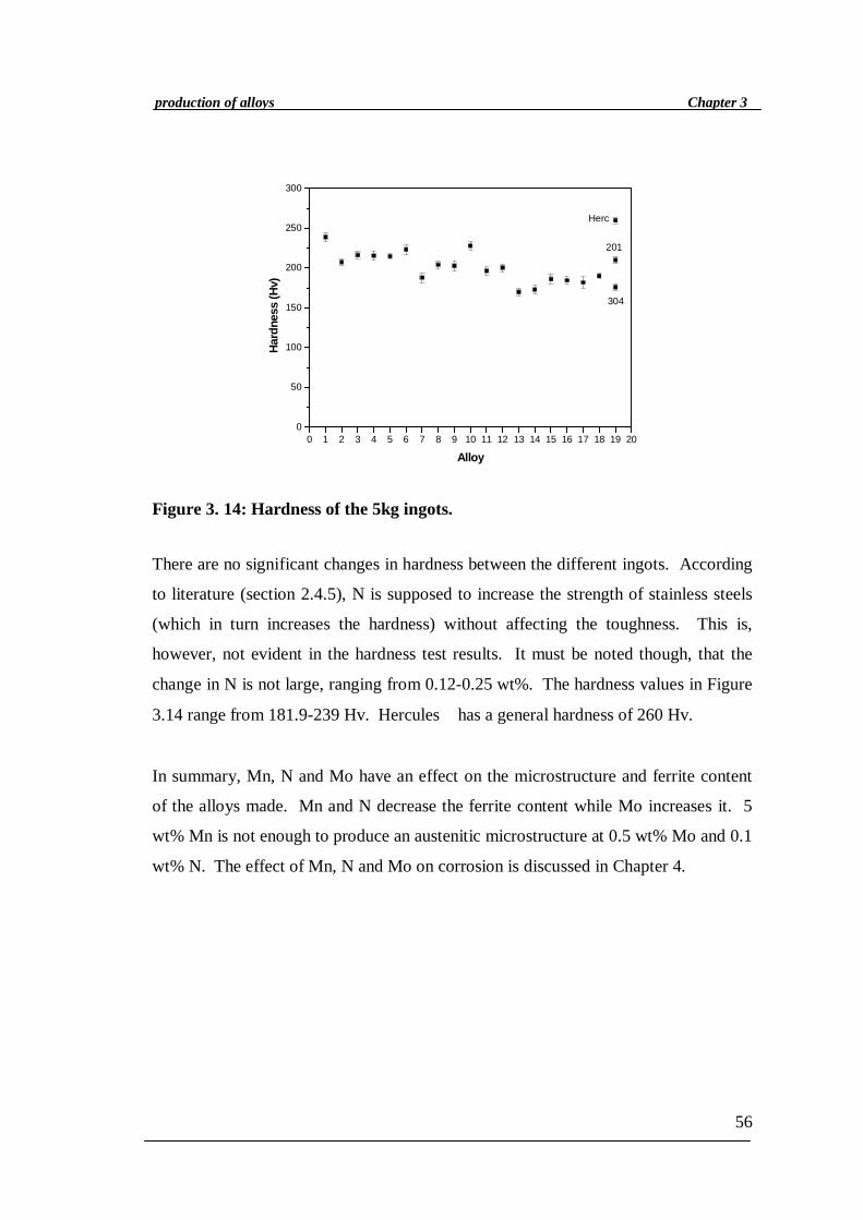
56
Chapter 3production of alloys
0 1 2 3 4 5 6 7 8 9 10 11 12 13 14 15 16 17 18 19 200
50
100
150
200
250
300
Herc
201
304
Hard
ness
(Hv)
Alloy
Figure 3. 14: Hardness of the 5kg ingots.
There are no significant changes in hardness between the different ingots. According
to literature (section 2.4.5), N is supposed to increase the strength of stainless steels
(which in turn increases the hardness) without affecting the toughness. This is,
however, not evident in the hardness test results. It must be noted though, that the
change in N is not large, ranging from 0.12-0.25 wt%. The hardness values in Figure
3.14 range from 181.9-239 Hv. Hercules has a general hardness of 260 Hv.
In summary, Mn, N and Mo have an effect on the microstructure and ferrite content
of the alloys made. Mn and N decrease the ferrite content while Mo increases it. 5
wt% Mn is not enough to produce an austenitic microstructure at 0.5 wt% Mo and 0.1
wt% N. The effect of Mn, N and Mo on corrosion is discussed in Chapter 4.
57
Chapter 4
4. Effect of alloying elements on corrosion behaviour
of Hercules-based alloys
After chemical and microstructural analyses of the eighteen alloys, general corrosion
testing was conducted on them to determine the effect of the varying amounts, and
combinations, of Mn, N and Mo on the corrosion rate and behaviour of the alloys.
The procedure and results are discussed in this chapter.
4.1 Testing procedure for general corrosion
The buttons and ingots were in the same condition prior to testing since they had all
been heated into the austenic region and then air cooled as discussed in section 3.2.
To determine the general corrosion behaviour of the alloys, corrosion tests were
carried out using potentiodynamic testing methods on a 600-grit ground surface and
in a 5 wt% sulphuric acid solution. A three-electrode corrosion cell consisting of a
working electrode, reference electrode and counter electrode was used to carry out the
corrosion tests. A saturated calomel electrode was used in all cases as the reference
electrode. There were slight differences in the corrosion cell set-up used to test the
buttons and ingots, these are discussed below. The experimental procedure followed
for testing the buttons and ingots for corrosion is listed in Table 4.1.

58
Chapter 4effect of alloying elements
Table 4. 1: Testing procedure for general corrosion of the alloys.
50g buttons 5 kg ingots
Solution 5 wt% H2SO4 5 wt% H2SO4
Environment Naturally aerated, static solution at room temperature Naturally aerated, static solution at 25°C.
Scan range The scan was started at -600mV vs. SCE and stopped
at 1200 mV vs. SCE
The scan was started at –600 mV and stopped at 1200mV
vs. SCE .
Scan rate 60 mV/min 10 mV/min
Reference
electrode
Saturated calomel electrode (SCE) Saturated calomel electrode (SCE)
Counter
electrode (CE)
Platinum wire Graphite electrode
Workingelectrode
(WE)
Test piece was clamped directly to the corrosion cell
using a carbon steel nail for electrical contact.
The 5kg ingots were machined into 5 mm diameter
cylindrical buttons, which were mounted into a sample
holder and immersed in the solution
Corrosion cell
Description of
testconditions
The reference electrode was housed in a Luggin-Haber
Capillary. To minimise error due to IR-losses the capillary
was place about 1cm from the working electrode. The alloy
surface was cleaned by conditioning at -700 mV for 600
seconds prior to scanning to ensure that a reproducible
surface was achieved for all alloys to be tested
The corrosion cell was placed in a water bath to keep the solution
at 25ºC. The alloys were not stabilized prior to testing so as to
avoid stabilization in the passive range since this would yield
much lower corrosion rates than desired. The alloys were also not
conditioned.
Potentiostat Schlumberger FI1286 ACM Instruments AutoTafel potentiostat
All scans were done in duplicate and the results obtained are discussed in section 4.2.
Platinumwire as
CE
Sample
Luggin probehousing SCE
Carbon stee l nail
H2SO4solution
Carbonrods as
theCE’s
Sample insample holder
Luggin probehousing the
SCE
H2SO4
solution

59
Chapter 4effect of alloying elements
4.2 Results of corrosion tests
The results of the buttons and the ingots are discussed together for comparison
purposes. Scans obtained for both buttons and ingots were similar in that they all had
more that one Ecorr as illustrated in Figure 4.1.
10-9 10-8 10-7 10-6 10-5 10-4 10-3 10-2 10-1-1.0
-0.5
0.0
0.5
1.0
1.5
Ecorr3
Ecorr2
Ecorr1
AC
A
C
Pote
ntia
l (V)
Current density (A/cm2)
Alloy 6a Alloy 6b
Figure 4. 1: Example of scans obtained for both ingots and buttons.
As shown in the figure, the scans had more than one cathodic “nose” at Ecorr’s 1, 2
and 3. These noses are due to the actual cathodic curve intersecting the actual anodic
curve more than once, as illustrated in Figure 4.2. (Figure 4.2 is merely an
illustration and is not drawn from values in Figure 4.1)
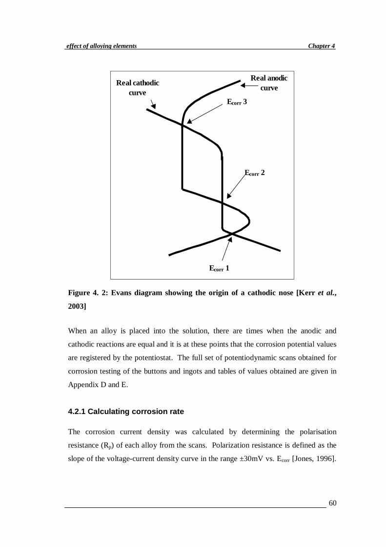
60
Chapter 4effect of alloying elements
Ecorr 3
Real anodiccurve
Ecorr 1
Ecorr 2
Real cathodiccurve
Figure 4. 2: Evans diagram showing the origin of a cathodic nose [Kerr et al.,
2003]
When an alloy is placed into the solution, there are times when the anodic and
cathodic reactions are equal and it is at these points that the corrosion potential values
are registered by the potentiostat. The full set of potentiodynamic scans obtained for
corrosion testing of the buttons and ingots and tables of values obtained are given in
Appendix D and E.
4.2.1 Calculating corrosion rate
The corrosion current density was calculated by determining the polarisation
resistance (Rp) of each alloy from the scans. Polarization resistance is defined as the
slope of the voltage-current density curve in the range ±30mV vs. Ecorr [Jones, 1996].
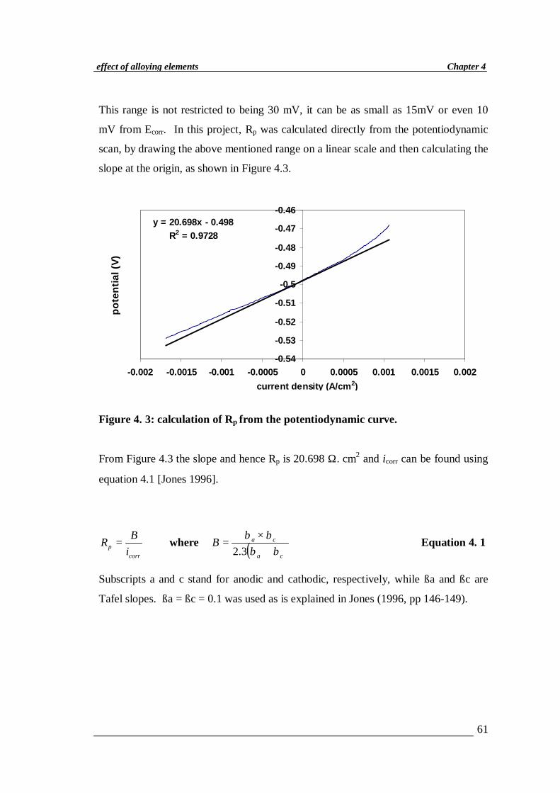
61
Chapter 4effect of alloying elements
This range is not restricted to being 30 mV, it can be as small as 15mV or even 10
mV from Ecorr. In this project, Rp was calculated directly from the potentiodynamic
scan, by drawing the above mentioned range on a linear scale and then calculating the
slope at the origin, as shown in Figure 4.3.
y = 20.698x - 0.498R2 = 0.9728
-0.54
-0.53
-0.52
-0.51
-0.5
-0.49
-0.48
-0.47
-0.46
-0.002 -0.0015 -0.001 -0.0005 0 0.0005 0.001 0.0015 0.002current density (A/cm2)
pote
ntia
l (V)
Figure 4. 3: calculation of Rp from the potentiodynamic curve.
From Figure 4.3 the slope and hence Rp is 20.698 Ω. cm2 and icorr can be found using
equation 4.1 [Jones 1996].
corrp i
BR = where ( )ca
caBββ
ββ+
×=
3.2 Equation 4. 1
Subscripts a and c stand for anodic and cathodic, respectively, while ßa and ßc are
Tafel slopes. ßa = ßc = 0.1 was used as is explained in Jones (1996, pp 146-149).

62
Chapter 4effect of alloying elements
4.2.2 Corrosion rate as a function of Mn, N and Mo content
icorr values obtained from the corrosion test results of the alloys were converted to
mm/y as described in section 2.2.1 and the results were as in figures 4.4 to 4.6.
Tables of actual corrosion values are tabulated in Appendix D (Table D1) and
Appendix E (Table E1). At this point it was important to observe the trends that Mo,
N and Mn had on the corrosion rate, ipass and icrit. Although AISI 304 and Hercules
were tested for corrosion for the ingots, AISI 201 was not yet available for testing. It
was thus decided to use reference values from literature for ease of comparison of the
ingots and button results. The values as indicated in the following graph are as cited
in Moema and Jones, 2005. Reference alloys were however tested in Chapter 5.
0.0 0.5 1.0 1.5 2.00
5
10
15
20
25
30
35
40
0.13 N0.21 N0.145 N
0.14 N0.16 N
0.20 N
0.12 N
0.12 N
0.12 N
0.17 N0.17 N
0.18 N
201
304
Herc
corr
osio
n ra
te (m
m/y
r)
wt% Mo
buttons ingots
Figure 4. 4: Corrosion rate of 5 wt% Mn buttons and alloys.
For both buttons and ingots, an increase in molybdenum, at 5 wt% Mn, seems to lead
to a decrease in the corrosion rate of the alloys (Figure 4.4). The corrosion values at
5 wt% Mn were higher for the 0.5 and 1 wt% Mo buttons and ingots than for those
having molybdenum content greater than 1.5 wt%. An increase in nitrogen also
seems to decrease corrosion rate except at the 0.5 wt% Mo level. Nitrogen does not,
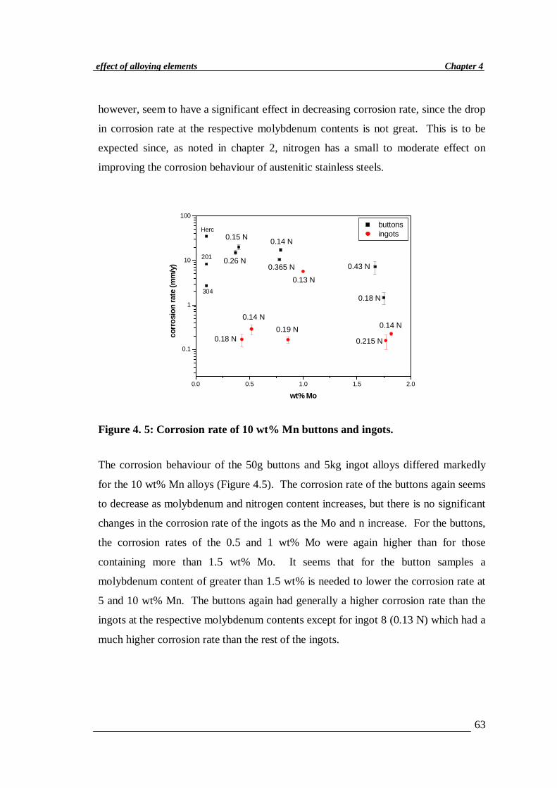
63
Chapter 4effect of alloying elements
however, seem to have a significant effect in decreasing corrosion rate, since the drop
in corrosion rate at the respective molybdenum contents is not great. This is to be
expected since, as noted in chapter 2, nitrogen has a small to moderate effect on
improving the corrosion behaviour of austenitic stainless steels.
0.0 0.5 1.0 1.5 2.0
0.1
1
10
100
0.14 N
0.215 N
0.13 N
0.19 N0.14 N
0.18 N
0.18 N
0.43 N0.365 N
0.14 N
0.26 N
0.15 NHerc
304
201
corr
osio
n ra
te (m
m/y
)
wt% Mo
buttons ingots
Figure 4. 5: Corrosion rate of 10 wt% Mn buttons and ingots.
The corrosion behaviour of the 50g buttons and 5kg ingot alloys differed markedly
for the 10 wt% Mn alloys (Figure 4.5). The corrosion rate of the buttons again seems
to decrease as molybdenum and nitrogen content increases, but there is no significant
changes in the corrosion rate of the ingots as the Mo and n increase. For the buttons,
the corrosion rates of the 0.5 and 1 wt% Mo were again higher than for those
containing more than 1.5 wt% Mo. It seems that for the button samples a
molybdenum content of greater than 1.5 wt% is needed to lower the corrosion rate at
5 and 10 wt% Mn. The buttons again had generally a higher corrosion rate than the
ingots at the respective molybdenum contents except for ingot 8 (0.13 N) which had a
much higher corrosion rate than the rest of the ingots.
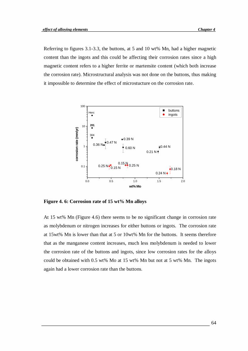
64
Chapter 4effect of alloying elements
Referring to figures 3.1-3.3, the buttons, at 5 and 10 wt% Mn, had a higher magnetic
content than the ingots and this could be affecting their corrosion rates since a high
magnetic content refers to a higher ferrite or martensite content (which both increase
the corrosion rate). Microstructural analysis was not done on the buttons, thus making
it impossible to determine the effect of microstucture on the corrosion rate.
0.0 0.5 1.0 1.5 2.0
0.1
1
10
100
Herc
201
304
0.15 N 0.25 N0.18 N
0.24 N
0.44 N0.21 N
0.60 N
0.39 N
0.15 N0.25 N
0.47 N0.36 N
corr
osio
n ra
te (m
m/y
r)
wt% Mo
buttons ingots
Figure 4. 6: Corrosion rate of 15 wt% Mn alloys
At 15 wt% Mn (Figure 4.6) there seems to be no significant change in corrosion rate
as molybdenum or nitrogen increases for either buttons or ingots. The corrosion rate
at 15wt% Mn is lower than that at 5 or 10wt% Mn for the buttons. It seems therefore
that as the manganese content increases, much less molybdenum is needed to lower
the corrosion rate of the buttons and ingots, since low corrosion rates for the alloys
could be obtained with 0.5 wt% Mo at 15 wt% Mn but not at 5 wt% Mn. The ingots
again had a lower corrosion rate than the buttons.
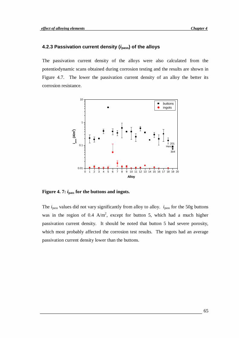
65
Chapter 4effect of alloying elements
4.2.3 Passivation current density (ipass) of the alloys
The passivation current density of the alloys were also calculated from the
potentiodynamic scans obtained during corrosion testing and the results are shown in
Figure 4.7. The lower the passivation current density of an alloy the better its
corrosion resistance.
0 1 2 3 4 5 6 7 8 9 10 11 12 13 14 15 16 17 18 19 200.01
0.1
1
10
Herc201
304
i pass
(A/m
2 )
Alloy
buttons ingots
Figure 4. 7: ipass for the buttons and ingots.
The ipass values did not vary significantly from alloy to alloy. ipass for the 50g buttons
was in the region of 0.4 A/m2, except for button 5, which had a much higher
passivation current density. It should be noted that button 5 had severe porosity,
which most probably affected the corrosion test results. The ingots had an average
passivation current density lower than the buttons.
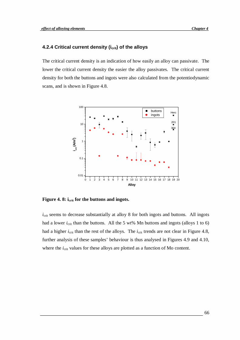
66
Chapter 4effect of alloying elements
4.2.4 Critical current density (icrit) of the alloys
The critical current density is an indication of how easily an alloy can passivate. The
lower the critical current density the easier the alloy passivates. The critical current
density for both the buttons and ingots were also calculated from the potentiodynamic
scans, and is shown in Figure 4.8.
0 1 2 3 4 5 6 7 8 9 10 11 12 13 14 15 16 17 18 19 200.01
0.1
1
10
100
Herc
304
201
i crit (
A/m
2 )
Alloy
buttons ingots
Figure 4. 8: icrit for the buttons and ingots.
icrit seems to decrease substantially at alloy 8 for both ingots and buttons. All ingots
had a lower icrit than the buttons. All the 5 wt% Mn buttons and ingots (alloys 1 to 6)
had a higher icrit than the rest of the alloys. The icrit trends are not clear in Figure 4.8,
further analysis of these samples’ behaviour is thus analysed in Figures 4.9 and 4.10,
where the icrit values for these alloys are plotted as a function of Mo content.
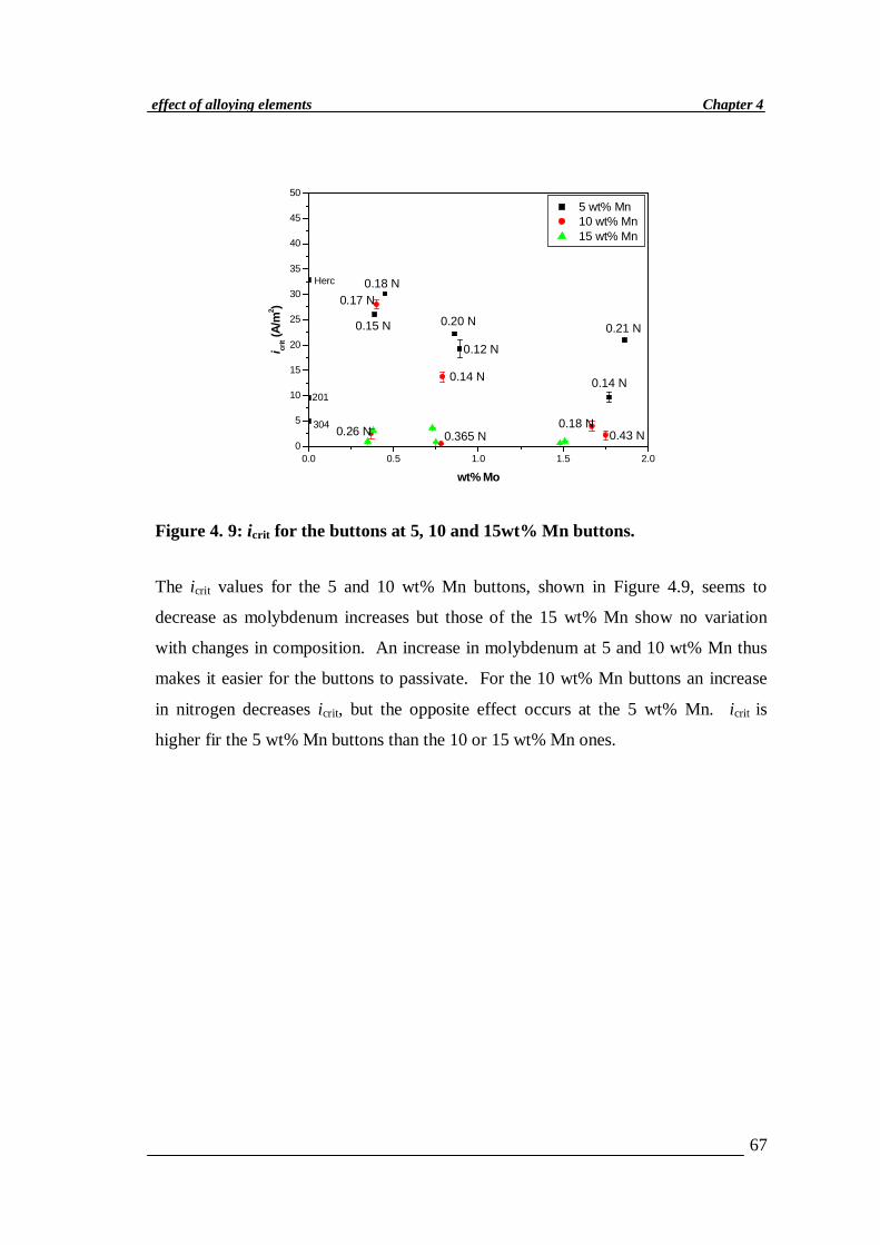
67
Chapter 4effect of alloying elements
0.0 0.5 1.0 1.5 2.00
5
10
15
20
25
30
35
40
45
50
0.43 N
Herc
201
304 0.26 N 0.365 N
0.18 N
0.14 N
0.21 N
0.14 N
0.12 N
0.20 N
0.18 N
0.15 N
0.17 N
i crit (
A/m
2 )
wt% Mo
5 wt% Mn 10 wt% Mn 15 wt% Mn
Figure 4. 9: icrit for the buttons at 5, 10 and 15wt% Mn buttons.
The icrit values for the 5 and 10 wt% Mn buttons, shown in Figure 4.9, seems to
decrease as molybdenum increases but those of the 15 wt% Mn show no variation
with changes in composition. An increase in molybdenum at 5 and 10 wt% Mn thus
makes it easier for the buttons to passivate. For the 10 wt% Mn buttons an increase
in nitrogen decreases icrit, but the opposite effect occurs at the 5 wt% Mn. icrit is
higher fir the 5 wt% Mn buttons than the 10 or 15 wt% Mn ones.
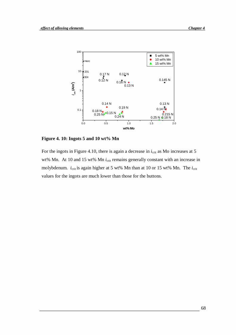
68
Chapter 4effect of alloying elements
0.0 0.5 1.0 1.5 2.0
0.1
1
10
100
0.25 N 0.24 N 0.25 N 0.18 N0.15 N 0.215 N
0.19 N0.18 N
0.14 N
0.13 N
0.14 N
0.145 N0.16 N
0.17 N
0.13 N
0.12 N
0.12 N
Herc
304
201
i crit (
A/m
2 )
wt% Mo
5 wt% Mn 10 wt% Mn 15 wt% Mn
Figure 4. 10: Ingots 5 and 10 wt% Mn
For the ingots in Figure 4.10, there is again a decrease in icrit as Mo increases at 5
wt% Mn. At 10 and 15 wt% Mn icrit remains generally constant with an increase in
molybdenum. icrit is again higher at 5 wt% Mn than at 10 or 15 wt% Mn. The icrit
values for the ingots are much lower than those for the buttons.
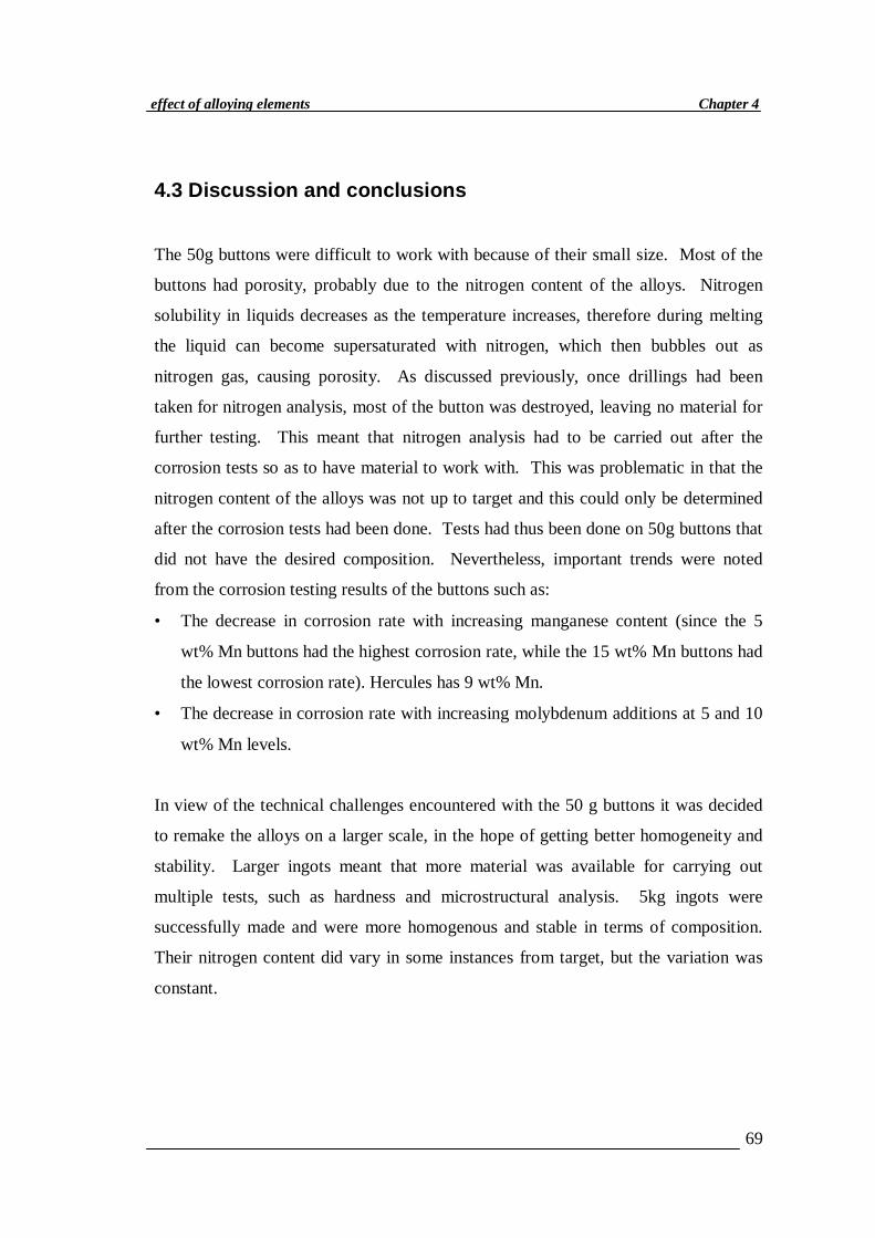
69
Chapter 4effect of alloying elements
4.3 Discussion and conclusions
The 50g buttons were difficult to work with because of their small size. Most of the
buttons had porosity, probably due to the nitrogen content of the alloys. Nitrogen
solubility in liquids decreases as the temperature increases, therefore during melting
the liquid can become supersaturated with nitrogen, which then bubbles out as
nitrogen gas, causing porosity. As discussed previously, once drillings had been
taken for nitrogen analysis, most of the button was destroyed, leaving no material for
further testing. This meant that nitrogen analysis had to be carried out after the
corrosion tests so as to have material to work with. This was problematic in that the
nitrogen content of the alloys was not up to target and this could only be determined
after the corrosion tests had been done. Tests had thus been done on 50g buttons that
did not have the desired composition. Nevertheless, important trends were noted
from the corrosion testing results of the buttons such as:
• The decrease in corrosion rate with increasing manganese content (since the 5
wt% Mn buttons had the highest corrosion rate, while the 15 wt% Mn buttons had
the lowest corrosion rate). Hercules has 9 wt% Mn.
• The decrease in corrosion rate with increasing molybdenum additions at 5 and 10
wt% Mn levels.
In view of the technical challenges encountered with the 50 g buttons it was decided
to remake the alloys on a larger scale, in the hope of getting better homogeneity and
stability. Larger ingots meant that more material was available for carrying out
multiple tests, such as hardness and microstructural analysis. 5kg ingots were
successfully made and were more homogenous and stable in terms of composition.
Their nitrogen content did vary in some instances from target, but the variation was
constant.

70
Chapter 4effect of alloying elements
From the corrosion test results of the ingots similar conclusions as those drawn for
the buttons could be made, such as a decrease in corrosion rate with increase in
manganese and molybdenum content. At 10 wt% Mn, the ingots behaved differently
from the buttons in that there was no change in corrosion behaviour with changes in
chemical composition for the ingots. 10 wt% Mn seems optimum for the ingots since
the 15 wt% Mn ingots behaved similarly.
Hercules (with no molybdenum and 0.25 wt% N) had a corrosion rate of 35 mm/y,
it thus seems that any addition of molybdenum or nitrogen can improve the corrosion
rate of Hercules since all the alloys tested (buttons and ingots) had lower corrosion
rates. The effect of nitrogen on the alloys is not clear from the corrosion test results,
but in the cases where it did lower corrosion rate, the decrease was not significant. It
should be noted though the variation in nitrogen was not large, ranging from 0.15 to
0.30 wt%.
Overall, the ingots were much more stable than the buttons. For this reason and the
fact that the current Hercules alloy has been developed for its mechanical properties
and changing its composition would markedly alter these properties, it was decided to
concentrate, in more detail on the 10 wt% Mn alloys, as discussed in the next chapter.
71
Chapter 5
5. The 10wt% Manganese ingots
From the results in the previous chapter (covering the overall corrosion behaviour of
the eighteen alloys) it was clear that the 10 wt% Mn alloys were of optimum
composition, also from a mechanical point of view, as mentioned. This chapter
therefore focuses solely on the 10 wt% Mn alloys with a detailed study of their
corrosion behaviour, benchmarked against those of AISI 304, 201 and Hercules.
The 10 wt% Mn alloys (ingots 7 to 12) were tested for general and pitting corrosion
using ASTM standards. Immersion tests were done, along with scanning electron
microscopy (SEM) analysis on the corroded surfaces to determine the mechanism of
corrosion. Results for reference alloys in this chapter are from actual tests done on
alloys AISI 201, AISI 304 and HerculesTM .
5.1 General corrosion of 10 wt% Mn ingots
Ingots 7 to 12 were tested for general corrosion behaviour according to ASTM
standard G5–94(2002) in a 5 wt% sulphuric acid solution at 30°C. The solution was
purged with nitrogen for an hour prior to scanning and also during scanning. The
alloys were ground to a 600-grit surface finish. A three-electrode corrosion cell was
once again used with carbon as the counter electrode and a saturated calomel
electrode (SCE) as the reference electrode. The scan was started at –200 mV vs. Ecorr
and ended at 1200 mV at a rate of 10mV/min. Two tests were performed per alloy.
Figure 5.1 is an example of a typical scan obtained during testing showing
reproducible results.
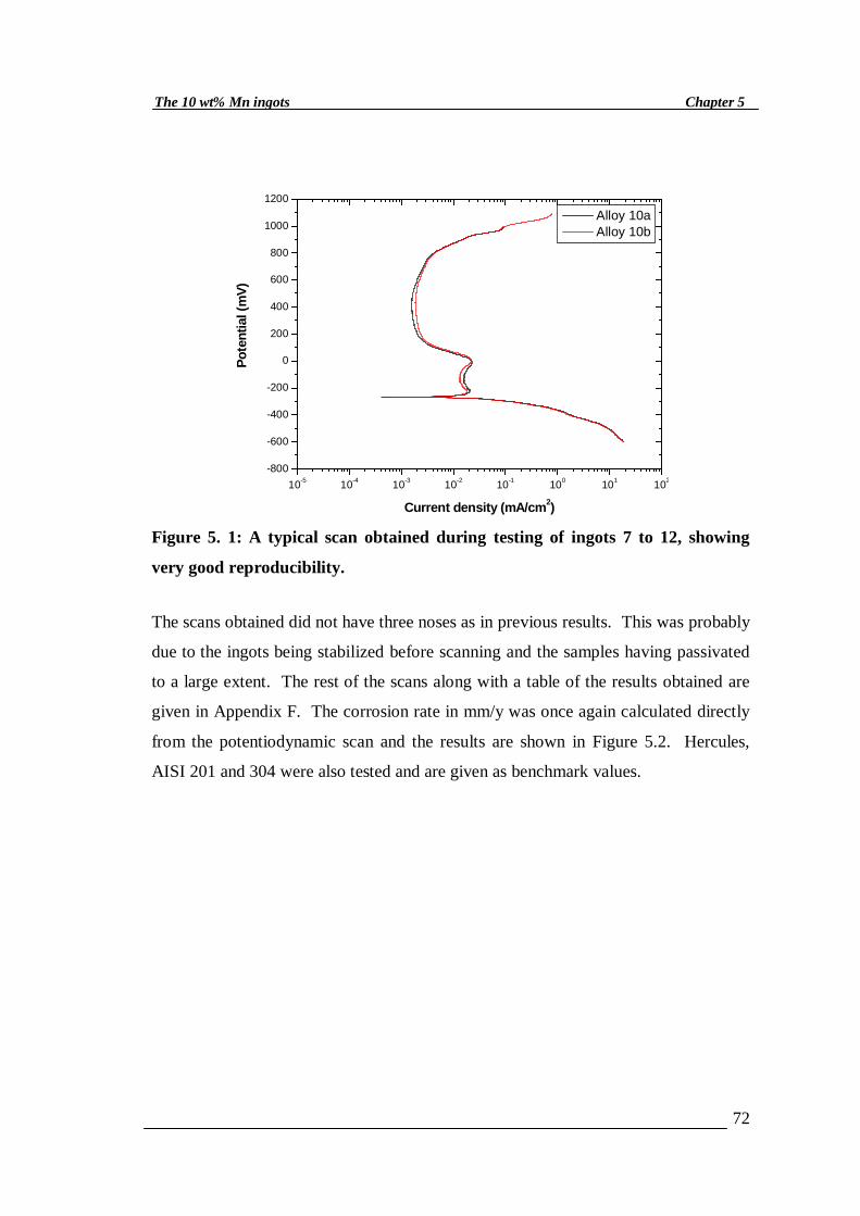
72
Chapter 5The 10 wt% Mn ingots
10-5 10-4 10-3 10-2 10-1 100 101 102-800
-600
-400
-200
0
200
400
600
800
1000
1200
Pote
ntia
l (m
V)
Current density (mA/cm2)
Alloy 10a Alloy 10b
Figure 5. 1: A typical scan obtained during testing of ingots 7 to 12, showing
very good reproducibility.
The scans obtained did not have three noses as in previous results. This was probably
due to the ingots being stabilized before scanning and the samples having passivated
to a large extent. The rest of the scans along with a table of the results obtained are
given in Appendix F. The corrosion rate in mm/y was once again calculated directly
from the potentiodynamic scan and the results are shown in Figure 5.2. Hercules,
AISI 201 and 304 were also tested and are given as benchmark values.

73
Chapter 5The 10 wt% Mn ingots
0.0 0.5 1.0 1.5 2.0
0.1
1
10
100
304
Herc
201
0.14 N
0.215 N
0.13 N0.19 N
0.14 N
0.18 NCorr
osio
n ra
te
wt% Mo
Figure 5. 2: Corrosion rate for ingots 7 to 12 as a function of Mo content.
The results verified what was found in previous tests, namely that no change in
corrosion rate at the 10 wt% Mn alloys occurs with changes in chemical composition.
The ingots had corrosion rates comparable to that of 304 and lower than Hercules
and 201. The corrosion rate of the ingots was low, ranging form 0.1 to 0.5 mm/y.
Hercules was found to have a corrosion rate of 24 mm/y (lower than in previous
tests) , and 201 was found to have a corrosion rate of 8 mm/y. The ingots had
nitrogen levels lower than Hercules (0.25 wt% N) but any combination of
molybdenum and nitrogen in the ingots still resulted in a much lower corrosion rate
than Hercules
Figure 5.3 shows all the scans obtained for ingots 7 to 12 on one graph so that the
effect of the alloying elements on the passivation and critical current densities of the
alloys can be illustrated.

74
Chapter 5The 10 wt% Mn ingots
10-5 10-4 10-3 10-2 10-1 100 101 102-800
-600
-400
-200
0
200
400
600
800
1000
1200
Pote
ntia
l (m
V)
Current density (mA/cm2)
0.18 N, 0.43 Mo 0.14 N, 0.52 Mo 0.19 N, 0.86 Mo 0.13 N, 1.00 Mo 0.215 N, 1.77 Mo 0.14 N, 1.82 Mo
Figure 5. 3: Full potentiodynamic scans of ingots 7 to 12 in 5 wt% H2SO4.
The passivation and critical current densities of the 10 wt% Mn alloys (Figure 5.3)
decreases as the molybdenum content increases. This is in agreement with literature
(section 2.4.4) where researchers found that molybdenum improves passivation and
general corrosion of stainless steel by decreasing these currents. Molybdenum thus
makes it easier for the alloy to passivate. Variations in nitrogen does not seem to
have a significant effect on the general corrosion of the 10 wt% Mn. No clear trend is
evident with changes in nitrogen content. The effect of changes in nitrogen on the
pitting potential of the 10 wt% Mn alloys was not clear. Actual pitting tests were
done to clarify this result as is discussed in the next section.
75
Chapter 5The 10 wt% Mn ingots
5.2 Pitting corrosion tests of 10 wt% Mn ingots
5.2.1 Pitting resistance equivalent (PRE) for the 10 wt% alloys
The pitting resistance equivalent (PRE), as mentioned in section 2.2.2, is a guide used
to predict the pitting resistance of stainless steel according to their chromium,
molybdenum and nitrogen content as in equation 5.1 [Frankel, 1998, Peckner and
Bernstein, 1977; Levey 1995]:
PRE = (%Cr) + 3.3(%Mo) + 16(%N) Equation 5. 1
The higher the pitting resistance of an alloy, the more resistant it is to pitting
corrosion [McEwan, 1994].
Figure 5.4 illustrates the PRE values for the six 10 wt% Mn alloys along with those
of Hercules, AISI 304 and 201.
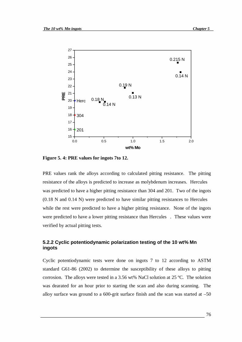
76
Chapter 5The 10 wt% Mn ingots
0.0 0.5 1.0 1.5 2.015
16
17
18
19
20
21
22
23
24
25
26
27
Herc
201
304
0.215 N
0.14 N
0.13 N
0.19 N
0.14 N
0.18 N
PRE
wt% Mo
Figure 5. 4: PRE values for ingots 7to 12.
PRE values rank the alloys according to calculated pitting resistance. The pitting
resistance of the alloys is predicted to increase as molybdenum increases. Hercules
was predicted to have a higher pitting resistance than 304 and 201. Two of the ingots
(0.18 N and 0.14 N) were predicted to have similar pitting resistances to Hercules
while the rest were predicted to have a higher pitting resistance. None of the ingots
were predicted to have a lower pitting resistance than Hercules. These values were
verified by actual pitting tests.
5.2.2 Cyclic potentiodynamic polarization testing of the 10 wt% Mningots
Cyclic potentiodynamic tests were done on ingots 7 to 12 according to ASTM
standard G61-86 (2002) to determine the susceptibility of these alloys to pitting
corrosion. The alloys were tested in a 3.56 wt% NaCl solution at 25 ºC. The solution
was dearated for an hour prior to starting the scan and also during scanning. The
alloy surface was ground to a 600-grit surface finish and the scan was started at –50

77
Chapter 5The 10 wt% Mn ingots
mV vs. Ecorr up to 1200 mV. Duplicate scans were done per sample. An example of a
typical scan is shown in Figure 5.5. The complete set of scans obtained is given in
Appendix G. and table of results.
10-7 10-6 10-5 10-4 10-3 10-2 10-1 100 101
-500
-400
-300
-200
-100
0
100
200
300
400
Pitting potential (Epit
)
Pote
ntia
l (m
V)
Current density (mA/cm2)
Pit 11a Pit 11b
Figure 5. 5: Example of cyclic scan obtained from pitting tests
All scans were reversed at 5 mA and all formed a hysterisis loop, as shown in Figure
5.5. The pitting potentials were read directly from the scan. These values are
represented graphically in Figure 5.6 as a function of Mo content.
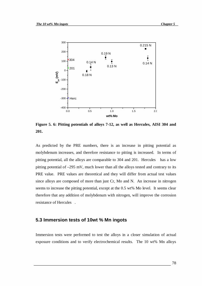
78
Chapter 5The 10 wt% Mn ingots
0.0 0.5 1.0 1.5 2.0-400
-300
-200
-100
0
100
200
300
Herc
201
304
0.215 N
0.14 N
0.19 N
0.13 N0.14 N
0.18 N
E pit (
mV)
wt% Mo
Figure 5. 6: Pitting potentials of alloys 7-12, as well as Hercules, AISI 304 and
201.
As predicted by the PRE numbers, there is an increase in pitting potential as
molybdenum increases, and therefore resistance to pitting is increased. In terms of
pitting potential, all the alloys are comparable to 304 and 201. Hercules has a low
pitting potential of –295 mV, much lower than all the alloys tested and contrary to its
PRE value. PRE values are theoretical and they will differ from actual test values
since alloys are composed of more than just Cr, Mo and N. An increase in nitrogen
seems to increase the pitting potential, except at the 0.5 wt% Mo level. It seems clear
therefore that any addition of molybdenum with nitrogen, will improve the corrosion
resistance of Hercules.
5.3 Immersion tests of 10wt % Mn ingots
Immersion tests were performed to test the alloys in a closer simulation of actual
exposure conditions and to verify electrochemical results. The 10 wt% Mn alloys

79
Chapter 5The 10 wt% Mn ingots
were thus tested in a 5 wt% sulphuric acid solution at room temperature in a naturally
aerated environment. The alloys were ground to a 120-grit surface finish, weighed
and measured before immersing in the solution on sample holders. The alloys were
weighed every 24 hours. After 14 days, the alloys were cleaned with a wire brush
and weighed again. The corrosion rate was then calculated with equation 5.2 [ASTM
standard G31-72 (2002)]
corrosion rate (mm/y) = tAD
WK××
× Equation 5. 2
Where K =8.76 x 10⁴, W = mass loss (g), D = density (g/cm3), A = surface area
(cm2), t = time (hrs)
5.3.1 Results of immersion tests
Figure 5.7 illustrates the mass loss experienced for the different ingots over the 14-
day immersion period. Readings were taken every 24 hours.
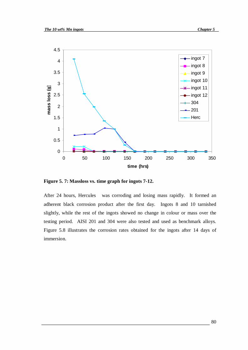
80
Chapter 5The 10 wt% Mn ingots
0
0.5
1
1.5
2
2.5
3
3.5
4
4.5
0 50 100 150 200 250 300 350
time (hrs)
mas
s lo
ss (g
)
ingot 7ingot 8ingot 9ingot 10ingot 11ingot 12304201Herc
Figure 5. 7: Massloss vs. time graph for ingots 7-12.
After 24 hours, Hercules was corroding and losing mass rapidly. It formed an
adherent black corrosion product after the first day. Ingots 8 and 10 tarnished
slightly, while the rest of the ingots showed no change in colour or mass over the
testing period. AISI 201 and 304 were also tested and used as benchmark alloys.
Figure 5.8 illustrates the corrosion rates obtained for the ingots after 14 days of
immersion.
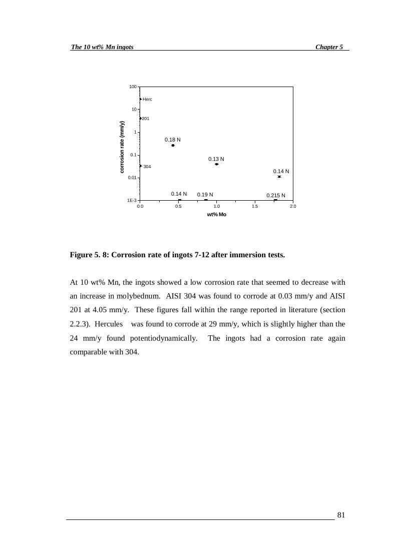
81
Chapter 5The 10 wt% Mn ingots
0.0 0.5 1.0 1.5 2.01E-3
0.01
0.1
1
10
100
0.215 N0.19 N
0.18 N
0.14 N
0.13 N
0.14 N
Herc
201
304
corr
osio
n ra
te (m
m/y
)
wt% Mo
Figure 5. 8: Corrosion rate of ingots 7-12 after immersion tests.
At 10 wt% Mn, the ingots showed a low corrosion rate that seemed to decrease with
an increase in molybednum. AISI 304 was found to corrode at 0.03 mm/y and AISI
201 at 4.05 mm/y. These figures fall within the range reported in literature (section
2.2.3). Hercules was found to corrode at 29 mm/y, which is slightly higher than the
24 mm/y found potentiodynamically. The ingots had a corrosion rate again
comparable with 304.
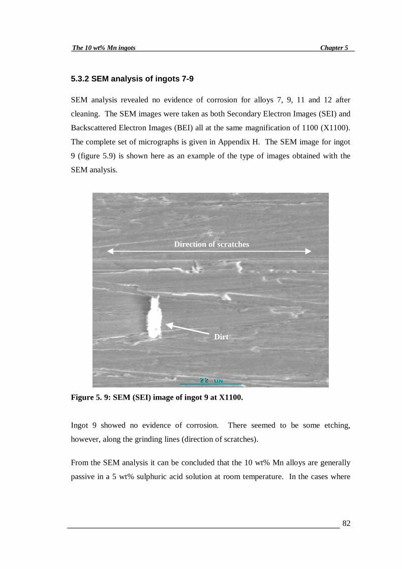
82
Chapter 5The 10 wt% Mn ingots
5.3.2 SEM analysis of ingots 7-9
SEM analysis revealed no evidence of corrosion for alloys 7, 9, 11 and 12 after
cleaning. The SEM images were taken as both Secondary Electron Images (SEI) and
Backscattered Electron Images (BEI) all at the same magnification of 1100 (X1100).
The complete set of micrographs is given in Appendix H. The SEM image for ingot
9 (figure 5.9) is shown here as an example of the type of images obtained with the
SEM analysis.
Direction of scratches
Dirt
Figure 5. 9: SEM (SEI) image of ingot 9 at X1100.
Ingot 9 showed no evidence of corrosion. There seemed to be some etching,
however, along the grinding lines (direction of scratches).
From the SEM analysis it can be concluded that the 10 wt% Mn alloys are generally
passive in a 5 wt% sulphuric acid solution at room temperature. In the cases where
83
Chapter 5The 10 wt% Mn ingots
they do corrode, the mechanism is general corrosion, except for ingot 8 (Appendix H)
which pitted. AISI 304 also showed pitting.
5.4 Discussion and Conclusions
From the potentiodynamic tests, it was found yet again that the 10 wt% Mn alloys
have low corrosion rates that are comparable to AISI 304. Potentiodynamic tests
showed Hercules to have a high corrosion rate of 24 mm/y. There was again no
change in corrosion rate as either molybdenum or nitrogen varied. This confirms
results obtained in previous tests. Immersion tests revealed that the mechanism of
corrosion in most instances was general corrosion, even though ingot 8 pitted. The
exposure time, however, was too short to make firm conclusions. More tests would
have to be done to determine when each type of corrosion occurs.
The 10 wt% ingots pitted in a 3.5 wt% NaCl solution at 25ºC, which is an
environment in which the alloys are susceptible to pitting. The tests revealed that the
higher the molybdenum content the more resistant the alloy was to pitting, as
predicted by the PRE values. An increase in nitrogen also increased resistance to
pitting.
Hercules again had a higher corrosion rate and a lower pitting resistance than the
rest of the alloys. Any addition of molybdenum with nitrogen therefore seems to
improve the corrosion resistance of this alloy.
84
Chapter 6
6. Summary and Conclusions
The aim of this project was to establish the effect of nitrogen, manganese and
molybdenum on the corrosion behaviour of low nickel austenitic stainless steels,
such as HerculesTM, developed by Mintek. A further aim was to find a
combination of these elements that will give a more corrosion resistant version of
HerculesTM. Preliminary tests were done on buttons and standard corrosion tests
on ingots. The alloys were made with a HerculesTM base composition with
variations in manganese, nitrogen and molybdenum. Manganese was varied in
three levels (5, 10 and 15 wt%), nitrogen in two levels (0.15 and 0.30 wt%) and
molybdenum in three levels (0.5, 1 and 2 wt%). Eighteen alloys were tested.
Compositional and microstructural analyses were done on the alloys along with
hardness, general corrosion, immersion and pitting tests. SEM analysis was done
after immersion testing.
From literature (Chapter 2) it was found that manganese can be used as a cheaper
substitute for nickel and that it aids nitrogen solubility. Researchers, however,
found manganese to weaken the passive film and form manganese sulphides
which assist in pit formation. Molybdenum and nitrogen were found by
researchers to improve both the general and pitting corrosion resistance of
stainless steels by decreasing the passivation current density and increasing the
pitting potential. Contrary to literature, actual potentiodynamic tests carried out
on the different buttons and ingots (Figure 4.4-4.6), showed that an increase in
manganese decreased the general corrosion rate of Hercules TM. In all alloys
tested the 15 wt% Mn alloys had the lowest corrosion rate while the 5 wt% Mn
alloys had the highest corrosion rate. Ferritescope readings (Figure 3.12)
illustrated that an increase in manganese generally decreased the ferrite content of
the alloys..
85
Chapter 6Summary and conclusions
This is to be expected since manganese is an austenite former and an increase in
this element would decrease the ferrite content of the alloys. Manganese also aids
nitrogen solubility, which in turn stabilises the austenite and thus decreases the
ferrite content of the alloys. Additions of manganese beyond 5 wt% thus
decreases the corrosion rate due to an increased austenite stability. 10 wt% Mn,
was the optimum in achieving significantly low corrosion rates of HerculesTM,
even with 0.5 wt% Mo.
It can thus be concluded that reducing the manganese content below 10 wt%
would produce alloys that have higher corrosion rates. Increasing the manganese
content beyond 10 wt% has no significant effect in reducing the corrosion rate of
HerculesTM since the 15 wt% Mn alloys behaved similarly to the 10 wt% Mn ones.
The current HerculesTM alloy has no molybdenum addition. Molybdenum proved,
however very effective in decreasing the corrosion rate of HerculesTM especially
at 5 wt% Mn (Figure 4.4-4.6). At this level of Mn an increase in molybdenum,
decreased the corrosion rate of HerculesTM from values around 20 mm/y down to
about 5 mm/y and lower, with the larger molybdenum contents (2 wt% Mo)
resulting in the lowest corrosion rate.
Any addition of molybdenum to the 10 and 15 wt% Mn alloys reduced the
corrosion rate significantly. Varying the amount of Mo added at these levels of
Mn did not however vary the corrosion rate behaviour which remained low and
constant irrespective of the increasing molybdenum contents. The buttons
differed from the ingots at the 10 wt% Mn level (Figure 4.5) by having a higher
corrosion rate. The corrosion rate of the buttons at 10 wt% Mn decreased with
increasing molybdenum whereas that for the ingots remained low and constant. .
Additions of molybdenum affected the ferrite content of the ingots. An increase
in molybdenum additions generally increased the ferrite content of the alloys
(Figure 3.13) as is to be expected since molybdenum is a strong ferrite former.
Results further showed that molybdenum decreased the passivation and critical
86
Chapter 6Summary and conclusions
current densities of the 10 wt% Mn ingots (Figure 5.3), as is found in literature.
Molybdenum thus improves corrosion rate by aiding the alloys to passivate easier
and lowering the passivation current, and leads to increased pitting potentials
(Figure 5.6). Molybdenum was more effective in improving the pitting resistance
of HerculesTM than the general corrosion resistance of the alloy, which did not
vary significantly with change in Mo content (Figure 5.2). Pitting potentials were
improved in such a way that the values were compatible with AISI 304, one of the
benchmark alloys in this project.
The addition of molybdenum thus improves the corrosion and pitting resistance of
HerculesTM, since at 10 wt% Mn, all alloys tested had a lower corrosion rate than
HerculesTM. Low corrosion rates can be attained with as little as 0.5 wt% Mo at
the 10 wt% Mn level (Figure 5.2).
HerculesTM has 0.25 wt% N, but all the ingots tested had lower nitrogen levels
(Figure 3.6). At 10 wt% Mn, increasing the nitrogen content of the ingots from
0.13 to 0.215 wt% had no effect on the corrosion rate (Figures 4.5 and 5.2). The
corrosion rate remained low and constant as both nitrogen and molybdenum
increased. The same behaviour is observed at the 15 wt% Mn level (Figure 4.6).
At 5 wt% Mn (Figure 4.4), however, higher nitrogen levels resulted in a lower
corrosion rate only at the 1 wt% Mo level.
Nitrogen levels greater than 0.25 wt% could only be attained with the buttons
(Figure 3.6) at the 10 and 15 wt% Mn levels. This is probably due to the
manganese aiding nitrogen solubility at these levels. At 10 wt% Mn (Figure 4.5)
an increase in nitrogen content resulted in a lower corrosion rate at molybdenum
contents less than 1.5 wt%. This is probably due to the nitrogen being an
austenite former and stabiliser. At higher molybdenum contents, however,
increasing the nitrogen content to 0.43 wt% increased the corrosion rate of the
buttons. This could be due to the nitrogen solubilty limit being reached, causing
nitrides to form in the microstructures and thus decreasing the corrosion resistance
of the button. At 15 wt% Mn (Figure 4.6), however, low corrosion rates could be

87
Chapter 6Summary and conclusions
obtained in the buttons with 0.47 wt% N and molybdenum contents less than 0.5
wt%. There is thus a synergism between nitrogen, molybdenum and manganese
in reducing the corrosion rate of HerculesTM.
HerculesTM with constant Mo and Mn values, but varying nitrogen levels, would
need to be made and tested to clarify the effect of nitrogen on corrosion rate. The
nitrogen range would perhaps have to be increased to include levels beyond those
of the present range if there was an interest in determining the actual effect of N
on the corrosion rate of HerculesTM. Nitrogen values between 0.1 and 0.5 wt%
could possibly be used to determine the solubility limit of nitrogen at the 10 wt%
Mn level.
No changes in passivation current densities were observed with changes in
nitrogen content (Figures 4.7). Critical current density decreased with increasing
Mo content at the 5 wt% Mn level for both buttons and ingots (Figures 4.8 to
4.10). There was a general decrease in icrit with an increase in Mo at the 10 wt%
Mn level for the buttons but not the ingots. Both the buttons and ingots showed to
changes in icrit with changes in Mo at 15 wt% Mn. It can thus again be said that
10 wt% Mn is optimum in decreasing the corrosion rate of Hercules™
significantly through a decrease in icrit which aids passivation.
An increase in nitrogen decreased the ferrite content of the HerculesTM alloys
(Figure 3.11). This is to be expected since nitrogen is an austenite former that
stabilises austenite and reduces the tendency for ferrite formation. An increasing
nitrogen content, increased the pitting resistance of the 10 wt% ingots at
molybdenum levels greater than 0.5 wt% (Figure 5.6). All alloys, however, had
higher pitting resistances than HerculesTM.
Immersion tests done on the 10 wt% Mn ingots confirmed that Hercules™ has a
high corrosion rate and that all other alloys tested had a much lower corrosion
rate. At 10 wt% Mn the ingots tested had low corrosion rates that decreased with
88
Chapter 6Summary and conclusions
increasing Mo content (Figure 5.8). SEM analysis revealed that in 5 wt%
sulphuric acid, the alloys corroded mostly by general corrosion.
In tests performed thus far no changes in composition caused a change in hardness
in any of the low nickel austenitic stainless steels. All alloys tested had a similar
average hardness of about 200 Hv (Figure 3.14).
HerculesTM was found to have an average corrosion rate ranging from 24 mm/y-
29 mm/y. This was much higher than that of any of the other alloys tested. It can
thus be said that any addition of Mo can improve the corrosion rate of HerculesTM.
Varying the amount of molybdenum added however has no effect on the corrosion
rate. Low corrosion rates at 10 wt% Mn can be attained with nitrogen levels
lower than those of HerculesTM (0.25 wt%) with a molybdenum addition of less
than 0.5 wt%, provided the nitrogen content is below the nitrogen solubility limit.
An alloy with a HerculesTM base composition, a minimum additions of 0.5 wt%
Mo, 10 wt% Mn and 0.15 N would thus be a more corrosion resistant version of
HerculesTM.
The development of HerculesTM aimed at producing an alloy that was 25 %
cheaper than AISI 304. It has been calculated that HerculesTM would cost
R14.50/kg in bar form [White, 2005] which is 21% less than the cost of AISI 304
in bar form. The current HerculesTM composition does not contain molybdenum
and any additions of molybdenum will thus increase its cost. Molybdenum prices
are currently higher than nickel prices and just as unpredictable [Adanac, 2005],
see Appendix I, and it could therefore be more cost effective to find another
alloying addition or method to reduce the corrosion rate of HerculesTM.
89
7. References
Adanac-Moly-Corp (November, 2005), http://www.adanacmoly.com/,
Angel, T. (1954). Formation of Martensite in Austenitic Stainless steels: Effects of
Deformation, Temperature and Composition, Journal of The Iron and Steel Institute,
May 1954, pp. 165-174.
Audouard, J.P. (1993). Stainless Steels, Les Editions de Physique Les Ulis, France,
.pp. 254-301.
ASTM G65, pp 370-373
Avesta Sheffield. (1994). Corrosion Handbook for Stainless Steels: Corrosion Tables,
Sandvikens Tryckeri, Sweden pp. 59-62.
Baba, H., Kodama, T., and Katada, Y. (2002). Role of Nitrogen on the Corrosion
Behaviour of Austenitic Stainless steels, Corrosion Science, Vol. 44, Issue 10, Oct,
pp. 2393-2407.
Banerjee, M.K., Mukherjee, A.N.and Mukherjee, K.P. (1990). Potentiokinetic
Behaviour of Copper and Manganese Bearing Stainless steels, NML Technical
Journal, Vol. 32, Feb-Nov, pp. 11-17.
90
Bastidas, J.M., Torres, C.L., Cano, E. and Polo, J.L.(2002). Influence of
Molybdenum on Passivation of Polarised Stainless Steels in a Chloride Environment,
Corrosion Science, Vol. 44, Issue 3, Mar., pp. 625-633.
Blom, K.J and Degerbeck, J. (1983). Low Manganese Austenitic Stainless Steels has
Improved resistance to Pitting and Crevice Corrosion, Materials Performance, July,
pp. 52-54.
Brigham, R.J. and Tozer, E.W. (1974). Effect of Alloying Additions on the Pitting
Resistance of 18% Chromium Austenitic Stainless Steels, Corrosion, Vol. 30, May
1974, pp. 161-166.
-
Callister, Jr. W.D (1994). Materials Science and Engineering, An Introduction, John
Wiley and Sons, Inc.,USA, pp. 242, 361.
Colombier, L. and Hochman, J. (1965). Stainless and Heat Resisting Steels, Edward
Arnold (Publishers) Ltd, pp 65-106, 134.
Cortie M.B. (1995). Low Nickel Austenitic Stainless Steel, Mintek Patent (P 12500
Za/MVS MINTEK), November, pp. 1-35.
Fontana, M.G. and Greene, N.D. (1982). Corrosion Engineering, Second Edition, Mc
Graw Hill Publishers, pp. 51-54.
Frankel, G.S. (1998). Pitting Corrosion of Metals, J. Electrochem. Soc., Vol. 145, No.
6., June, pp. 2186-2197.
Gross, C.J. and Robinson, F.P.A. (1981). Effect of the Addition of up to 18%
Manganese on the Microstructure and Corrosion Properties of a 14.5% Chromium
91
references
Stainless Steel, Metallic Corrosion, Proceedings-31st International Congress on
Metallic Corrosion, South Africa,Vol. 1, pp. 114.
Gross, C. J. (1980). The Effect of Manganese on the Structure and Corrosion
Properties of 14.5% Chromium Stainless Steels, MSc Dissertation, January,
University of the Witwatersrand, Department f Metallurgy,pp. 14, 61, 62.
Hajjaji, S.E., Aries, L., Audouard, J.P. and Dabosi, F. (1995). The Influence of
Alloying Elements on the Corrosion Resistance of Stainless Steels in Phosphoric
Acid Medium Polluted by Sulphide Ions, Corrosion Science, Vol. 37, No. 6, pp. 927-
939.
Harvey, P.D. (1982). Engineering Properties of Steel, American Society For Metals,
U.S.A, pp. 246-281.
Hashmito, K. and Asami, K. (1979). An X-ray Photoelectron Spectroscopic Study of
the Passivity of Ferritic 19Cr-Stainless Steels in HCL, Corrosion Science, Vol. 19,
pp. 251, 1979.
Ilevbare, G.O. and Burstein, G.T. (2001). The Role of Alloyed Molybdenum in the
Inhibition of Pitting Corrosion in Stainless Steels, Corrosion Science, Vol. 43, pp.
485-513.
Iorio, L., Cortie, M. and Jones, R. (1994). Technical Data: Solubility of Nitrogen in
Experimental low-nickel Austenitic Stainless Steels, The Journal of The South
African Institute of Mining and Metallurgy, Vol. 94, no. 7, july, pp. 173-177.
Jargelius-Patterson, R.F.A. (1999). Electrochemical Investigation of the Influence of
Nitrogen on Pitting Corrosion of Austenitic Stainless Steels, Corrosion Science, Vol.
41, pp. 1639-1664.
92
references
Jargelius-Patterson, R.F.A. (1994). Phase Transformations in Manganese-Alloyed
Austenitic Stainless steel, Scripta Metallurgica et Materialia, Vol. 30, No. 9, pp.
1233-1238.
Jones, D.A., Principles and Prevention of Corrosion, Prentice-Hall, Inc., U.S.A., pp.
75-80, 143-153.
Kerr, J. (2003). New Generation Low-Nickel (≤2%) Austenitic Stainless Steels for
Structural Application, MINTEK Annual Report (C3785M ), pp. 1-2, 42-57.
Kincer, M.U and McEwan, J.J. (1993). Corrosion Testing of Stainless Steel,
Chemical Technology, Oct. 1993, pp. 7-9.
Levey, P.R.. (1995), The Mechanistic Involvement of Alloyed Nitrogen In The
Corrosion of Stainless Steel, MSc Dissertation, University of the Witwatersrand, pp.
3-30.
Lula, R.A. (1986), Manganese Stainless Steels, The Manganese Centre, France, pp.
22.43, 51-57.
McEwan, J.J. (1994). Corrosion Control in Southern Africa, Corrosion Institute of
Southern Africa, South Africa, pp. 25-26.
Moema, J.S., Paton, R. and Papo, M.J. (2005). On the Development of a New Low-
Nickel Stainless Steel for Structural and Long Product Application, Mintek
Publication (C4076M), Mintek, Randburg, South Africa, p. 1.
Newman, R.C. (2001). Understanding the Corrosion of Stainless Steel, Corrosion,
Vol. 57, No.12, pp. 1030-1041.
93
references
Paton, R., Oliver, D., McEwan, J.J.and Kerr, J. (2004). “AlphaGamma” Estimating
Microstructures and Properties in Stainless Steel Alloys, Revision 6, Advanced
Materials Division- January 1994, Mintek, Randburg, South Africa.
Peckner, D. and Bernstein, I.M. (1977). Handbook of Stainless Steels, Mc-Graw–Hill
Company, pp. 1-2, 4-3, 15-1-15-6.
Pickering, F.B. (1979). The Metallurgical Evolution of Stainless Steels, American
Society for Metals: The metals Society, pp. 23-39.
Raja, V.S., Davasenapathi, A., Veluchamy, P. and Minoura, H. (1999). Electron
Spectroscopy for Chemical Analysis Study of Corrosion Films Formed on
Manganese Stainless Steels, Corrosion, Vol. 55, No. 12, pp. 1119-1125.
Rama Rao, P. and Kutumbarao, V. (1989). Developments in Austenitic Steels
Containing Manganese, International Materials Reviews, Vol. 34, No. 2, pp. 69-85.
Rondelli, G., Vicentini, B. and Cigada, A. (1995). Influence of Nitrogen and
Manganese on Localised Corrosion Behaviour of Stainless Steels in Chloride
Environments, Materials and Corrosion, Vol. 46, pp. 628-632.
Schollenberger, H.J. (1995). The Effects of Delta Ferrite and Sigma Phase on the
Mechanical Properties and Corrosion Behaviour of 300 Series Austenitic Stainless
Steels, MSc Dissertation. March, Faculty of Engineering, University of The
Witwatersrand, Johannesburg, pp. 2-20.
Sedriks, A.J. (1979). Corrosion of Stainless Steels, John Wiley and Sons, Inc.,
Canada, pp. 9-21.
94
references
Sedriks, A.J. (1983). Role of sulphide Inclusions in Pitting and Crevice Corrosion of
Stainless Steels, International Metals Reviews, Vol. 28, No. 5, pp. 295-306.
Sedriks, A.J. (1986). National Association of Corrosion Engineers, vol. 42, July,No.
7, pp. 376-389.
Shams, A.M., Din, E.L., Badran, M.M. and Khalil, S.E. (1999) Corrosion Behaviour
of Manganese-Containing stainless Steels, Werkstoff und Korrosion, pp.50-56.
Simpson, J. (1990). Guideline on Electrochemical Corrosion Measurement, European
Federation of Corrosion, The Institute of Metals, London, pp. 37-39.
Sibanda, M, Vismer, S.L. and Knutsen, R.D. (1994). Consideration of Reduced
Nickel Containing Austenitic Stainless Steels for Forming Application, Materials
Letters 21, pp. 203-207.
Sumita, M., Hanawa T and Teoh, S.H. (2004). Development of Nitrogen- Containing
Nickel-Free Austenitic Stainless steels for Metallic Biomaterials, Materials Science
and Engineering:C, Vol. 24, issues 6-8, December, pp. 753-760.
Tretheway and Chamberlain (2002) Corrosion for Science and Engineering, 2nd
Edition, Longman, Harlow Essex.
Turan, Y.N. (1991). Effect on Nitrogen on the Structure and Properties of Type AISI
310 Austenitic stainless Steels, MSc Dissertation, University of the Witwatersrand,
Johannesburg.

95
references
Vismer, S.L. (1997). The Influence of Copper Addition on the Corrosion Behaviour
of Low-Nickel Austenitic Stainless Steels, MSc, University of Cape Town, Cape
Town.
Wellbeloved, D. and Stanko, J. (1990). Manganese – A Substitute for Nickel, Metals
Bulletin Monthly, January, pp. 61- 63.
White, R. (2005). Mintek Commercialisation plan-Project 32434, pp. 2-43.

96
Appendices
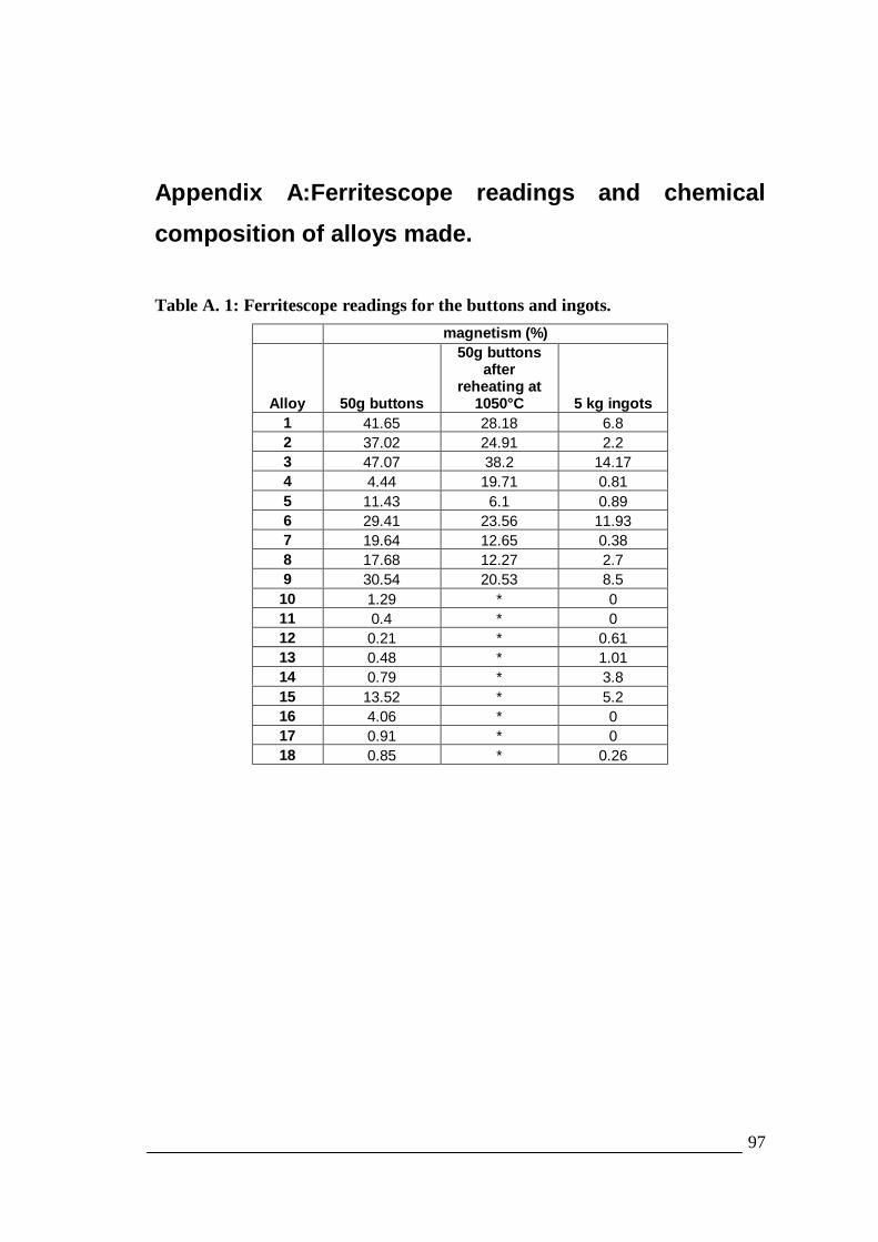
97
Appendix A:Ferritescope readings and chemicalcomposition of alloys made.
Table A. 1: Ferritescope readings for the buttons and ingots. magnetism (%)
Alloy 50g buttons
50g buttonsafter
reheating at1050°C 5 kg ingots
1 41.65 28.18 6.82 37.02 24.91 2.23 47.07 38.2 14.174 4.44 19.71 0.815 11.43 6.1 0.896 29.41 23.56 11.937 19.64 12.65 0.388 17.68 12.27 2.79 30.54 20.53 8.5
10 1.29 * 011 0.4 * 012 0.21 * 0.6113 0.48 * 1.0114 0.79 * 3.815 13.52 * 5.216 4.06 * 017 0.91 * 018 0.85 * 0.26
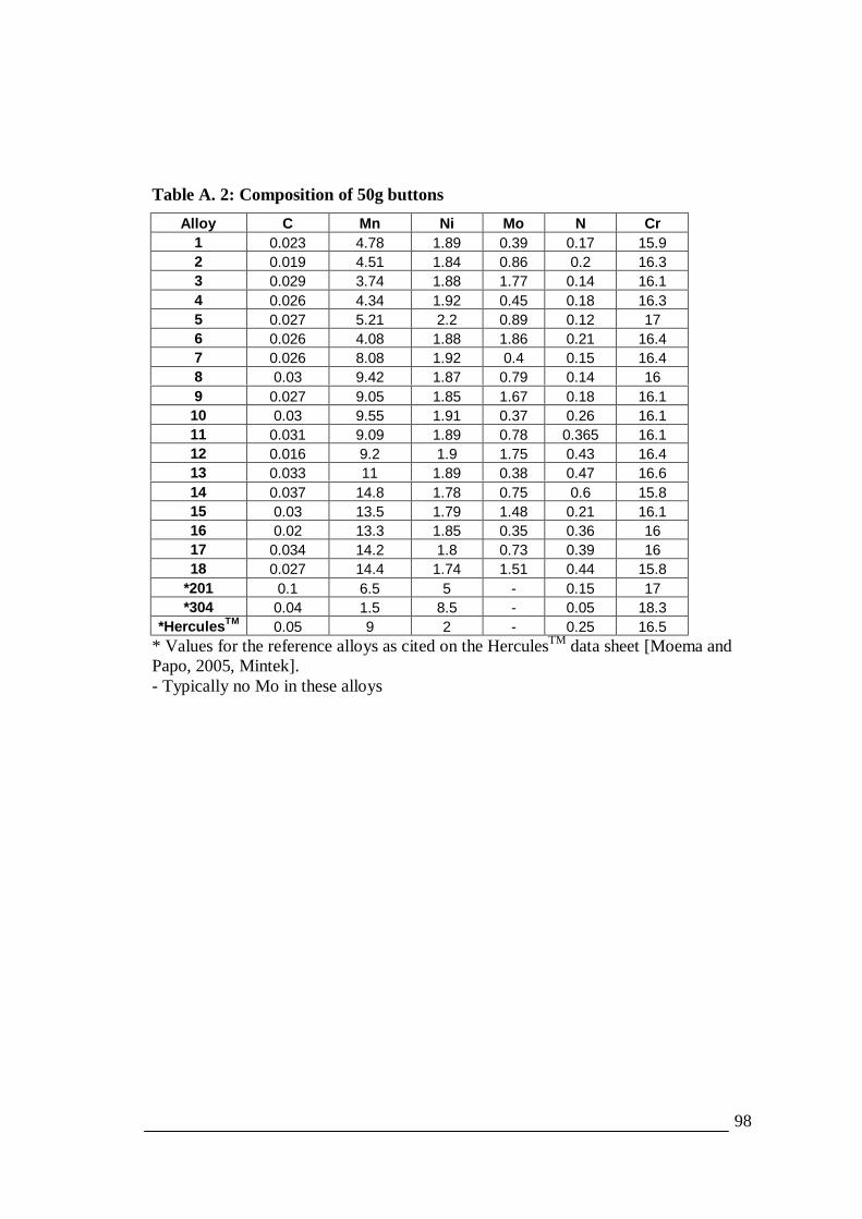
98
Table A. 2: Composition of 50g buttonsAlloy C Mn Ni Mo N Cr
1 0.023 4.78 1.89 0.39 0.17 15.92 0.019 4.51 1.84 0.86 0.2 16.33 0.029 3.74 1.88 1.77 0.14 16.14 0.026 4.34 1.92 0.45 0.18 16.35 0.027 5.21 2.2 0.89 0.12 176 0.026 4.08 1.88 1.86 0.21 16.47 0.026 8.08 1.92 0.4 0.15 16.48 0.03 9.42 1.87 0.79 0.14 169 0.027 9.05 1.85 1.67 0.18 16.1
10 0.03 9.55 1.91 0.37 0.26 16.111 0.031 9.09 1.89 0.78 0.365 16.112 0.016 9.2 1.9 1.75 0.43 16.413 0.033 11 1.89 0.38 0.47 16.614 0.037 14.8 1.78 0.75 0.6 15.815 0.03 13.5 1.79 1.48 0.21 16.116 0.02 13.3 1.85 0.35 0.36 1617 0.034 14.2 1.8 0.73 0.39 1618 0.027 14.4 1.74 1.51 0.44 15.8
*201 0.1 6.5 5 - 0.15 17*304 0.04 1.5 8.5 - 0.05 18.3
*HerculesTM 0.05 9 2 - 0.25 16.5* Values for the reference alloys as cited on the HerculesTM data sheet [Moema andPapo, 2005, Mintek].- Typically no Mo in these alloys

99
Table A. 3: Composition of 5 kg ingotsAlloy C Mn Ni Mo N Cr
1 0.036 5.02 2.19 0.44 0.12 15.42 0.036 4.89 2.21 0.92 0.12 15.63 0.03 5.02 2.09 1.79 0.13 15.74 0.031 4.91 2.22 0.45 0.17 15.65 0.034 4.92 2.1 0.85 0.16 15.76 0.036 5.42 1.98 1.79 0.145 15.87 0.027 9.33 2.1 0.52 0.14 15.98 0.019 9.12 2.09 1 0.13 15.79 0.028 9.36 2.11 1.82 0.14 15.7
10 0.032 8.93 2.24 0.43 0.18 15.511 0.028 9.04 2.19 0.86 0.19 15.912 0.043 9.09 2.21 1.77 0.215 1613 0.019 14.7 2.12 0.49 0.15 1614 0.021 15 2.15 0.84 0.15 16.215 0.024 15 2.23 1.73 0.18 15.816 0.029 15.4 2.23 0.46 0.25 15.917 0.028 15.8 2.2 0.8 0.24 15.918 0.038 15.5 2.21 1.67 0.25 16
*201 0.1 6.5 5 - 0.15 17*304 0.04 1.5 8.5 - 0.05 18.3
*HreculesTM 0.05 9 2 - 0.25 16.5* Values for the reference alloys as cited on the HerculesTM data sheet[Moema andPapo, 2005, Mintek].- Typically no Mo in these alloys
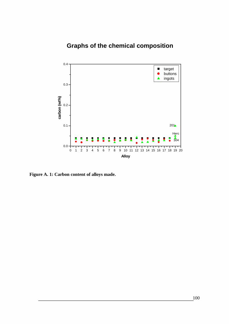
100
Graphs of the chemical composition
0 1 2 3 4 5 6 7 8 9 10 11 12 13 14 15 16 17 18 19 200.0
0.1
0.2
0.3
0.4
Herc
201
304
ca
rbon
(wt%
)
Alloy
target buttons ingots
Figure A. 1: Carbon content of alloys made.
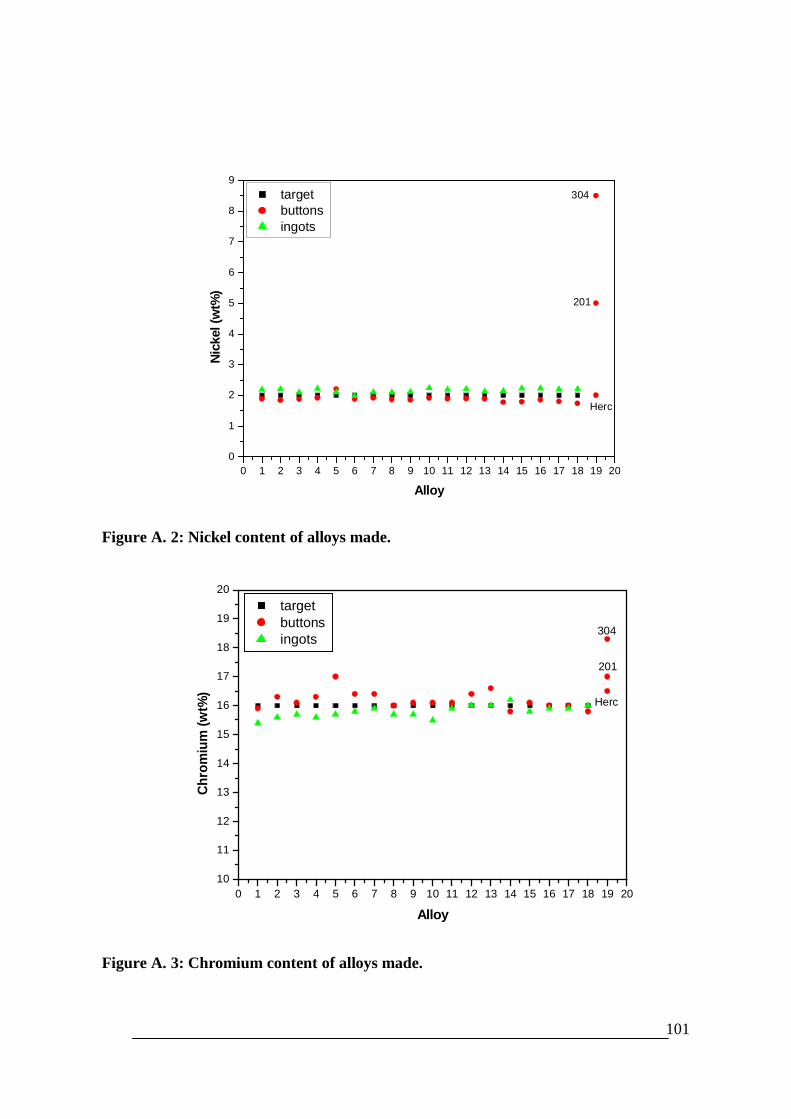
101
0 1 2 3 4 5 6 7 8 9 10 11 12 13 14 15 16 17 18 19 200
1
2
3
4
5
6
7
8
9
Herc
304
201
Nick
el (w
t%)
Alloy
target buttons ingots
Figure A. 2: Nickel content of alloys made.
0 1 2 3 4 5 6 7 8 9 10 11 12 13 14 15 16 17 18 19 2010
11
12
13
14
15
16
17
18
19
20
Herc
304
201
Chro
miu
m (w
t%)
Alloy
target buttons ingots
Figure A. 3: Chromium content of alloys made.
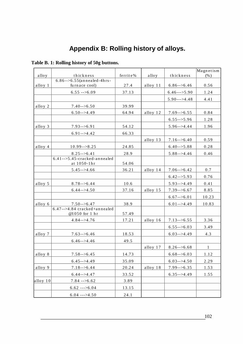
102
Appendix B: Rolling history of alloys.
Table B. 1: Rolling history of 50g buttons.
alloy thickness ferrite% alloy thicknessMagnetism
(%)
alloy 16.86-->6.55(annealed-4hrs-
furnace cool) 27.4 alloy 11 6.86-->6.46 0.56 6.55 -->6.09 37.13 6.46--->5.90 1.24 5.90--->4.48 4.41
alloy 2 7.40-->6.50 39.99 6.50-->4.49 64.94 alloy 12 7.69-->6.55 0.84 6.55-->5.96 1.28
alloy 3 7.93-->6.91 54.12 5.96-->4.44 1.96 6.91-->4.42 66.33 alloy 13 7.16-->6.40 0.59
alloy 4 10.99-->8.25 24.85 6.40-->5.88 0.28 8.25-->6.41 28.9 5.88-->4.46 0.46
6.41-->5.45-cracked-annealed
at 1050-1hr 54.06 5.45-->4.66 36.21 alloy 14 7.06-->6.42 0.7 6.42-->5.93 0.76
alloy 5 8.78-->6.44 10.6 5.93-->4.49 0.41 6.44-->4.50 37.16 alloy 15 7.39-->6.67 8.85 6.67-->6.01 10.23
alloy 6 7.50-->6.47 38.9 6.01-->4.49 10.83
6.47-->4.84 cracked+annealed
@1050 for 1 hr 57.49 4.84-->4.76 17.21 alloy 16 7.13-->6.55 3.36 6.55-->6.03 3.49
alloy 7 7.63-->6.46 18.53 6.03-->4.49 4.3 6.46-->4.46 49.5 alloy 17 8.26-->6.68 1
alloy 8 7.58-->6.45 14.73 6.68-->6.03 1.12 6.45-->4.49 35.09 6.03-->4.50 2.29
alloy 9 7.18-->6.44 20.24 alloy 18 7.99-->6.35 1.53 6.44-->4.47 33.52 6.35-->4.49 1.55
alloy 10 7.84 -->6.62 3.89
6.62 --->6.04 13.15
6.04 --->4.50 24.1

103
Table B. 2: Hardness of 5 kg ingots
*Values as cited in MINTEK communication C4105M pp. 50 [Moema and Papo,2005].
Alloyhardness
(Hv)1 2392 207.33 216.44 215.65 214.76 223.47 1888 204.29 202.6
10 22811 196.612 200.313 17014 17315 185.916 184.617 181.918 190.1
*201 210*304 176
*Hercules TM 260

104
Appendix C: Microstructural analysis of the ingots.
AlloyMicrostructure obtained using
10% oxalic acidMicrostructure obtained using
KOH
Alloy
1
Alloy2
Alloy3
α'
γγ
ά
γ
γ
α α
γα
α
γ
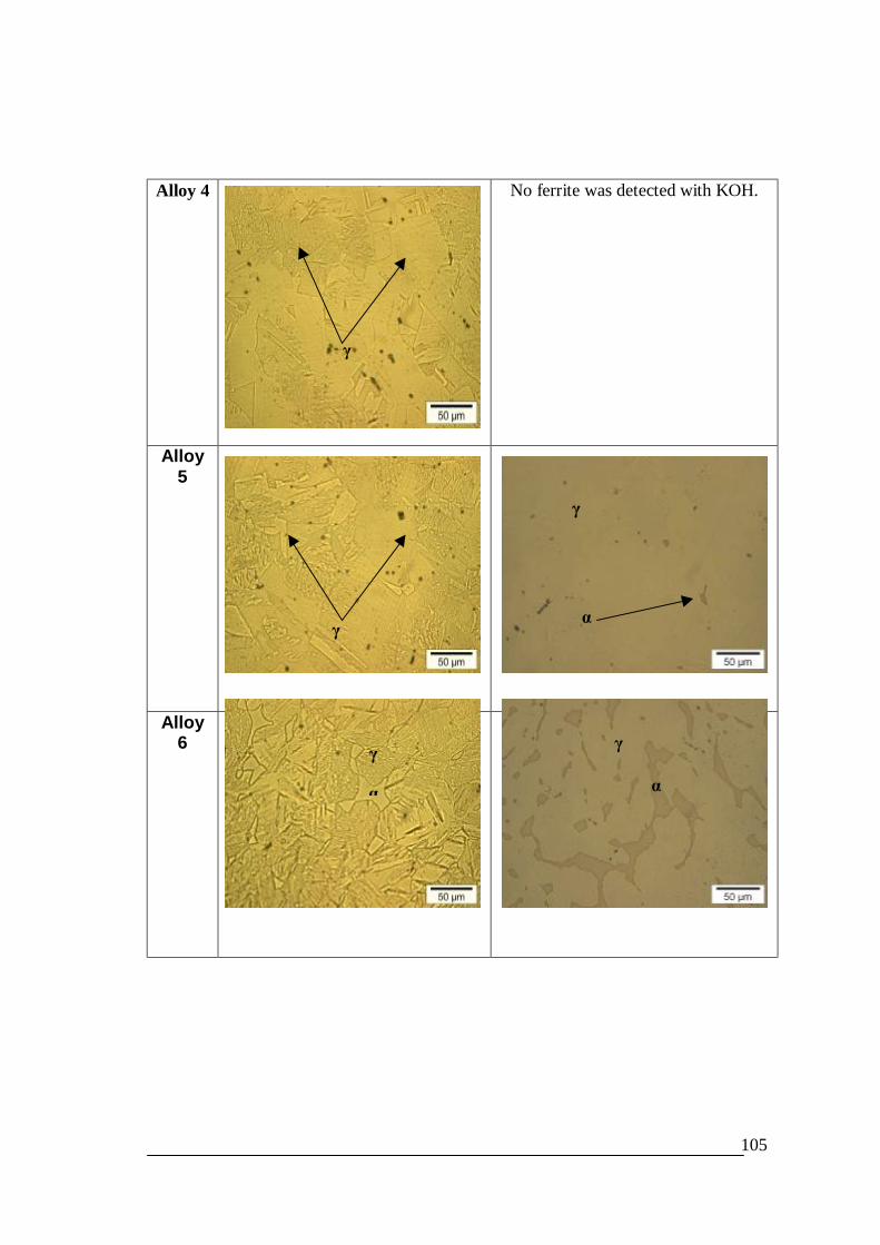
105
Alloy 4 No ferrite was detected with KOH.
Alloy5
Alloy6
α
γ γ
α
γ
γ
γ
α

106
Alloy 7
Alloy8
Alloy9
γ
γ
α
γ
α
γ
α
γ
αγ
α
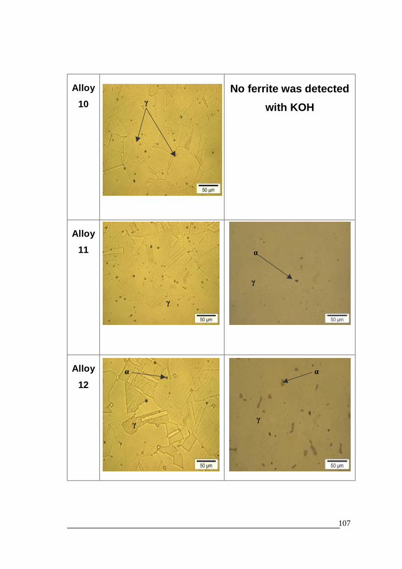
107
Alloy10
No ferrite was detectedwith KOH
Alloy11
Alloy
12
γ
α
γ
γ
α
γ
α
γ
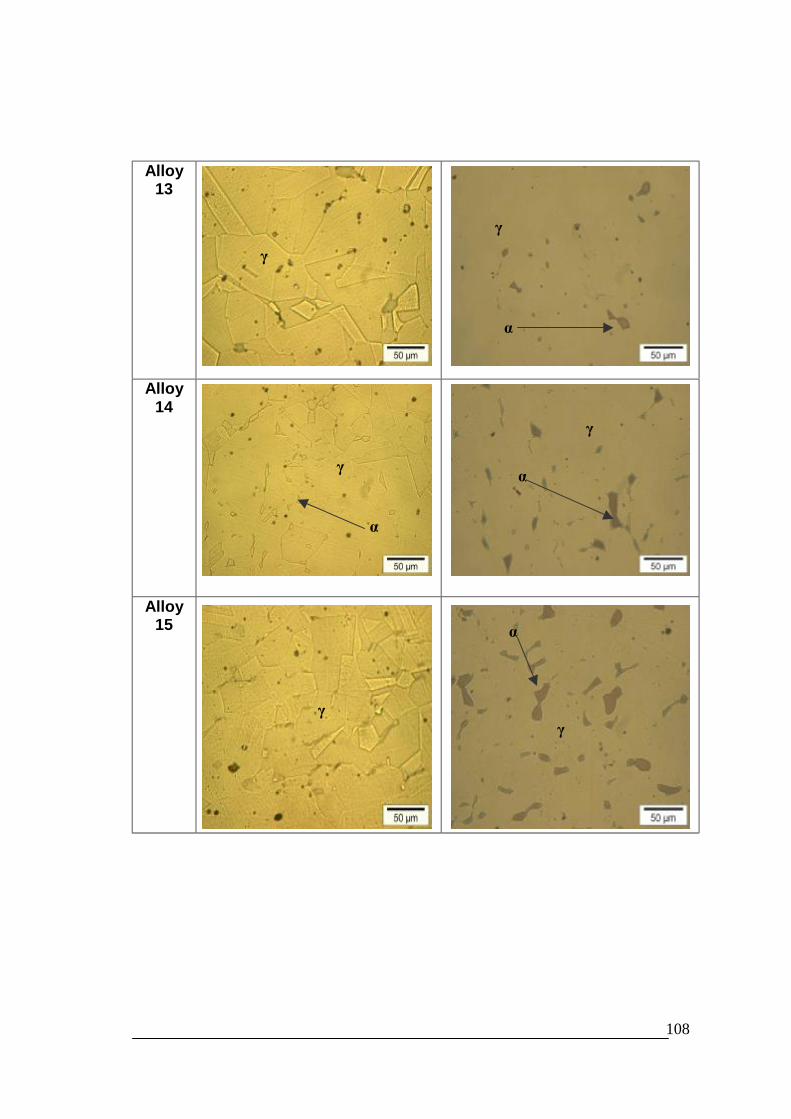
108
Alloy13
Alloy14
Alloy15
γ
γ
α
γ
α
γ
γ
α
α
γ
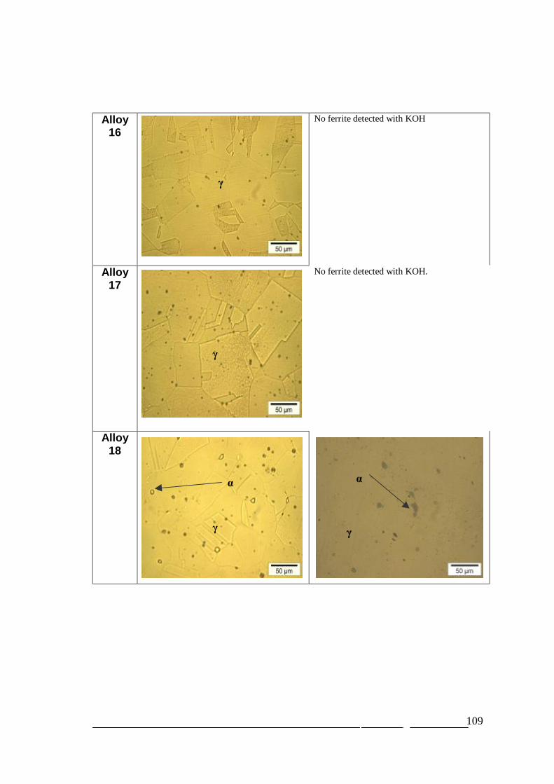
109
Alloy16
No ferrite detected with KOH
Alloy17
No ferrite detected with KOH.
Alloy18
γ
γ
γ
α α
γ

110
Appendix D: Results of potentiodynamic scansobtained for the buttons.
Table D. 1: Corrosion results for the 50g buttons.
alloycorrosion rate
(mm/y) Icorr(A/m2) Ipass (A/m2) icrit (A/m2)1 13.25 12.45 0.21 25.992 12.34 11.58 0.18 22.223 8.14 7.55 0.20 9.634 18.94 17.83 0.42 30.105 16.63 15.65 4.56 19.266 5.38 5.00 0.41 20.927 18.56 17.50 0.35 28.008 13.86 12.99 0.57 13.729 5.90 5.49 0.40 3.94
10 14.09 13.26 0.40 2.5211 10.63 9.89 0.24 0.4812 1.70 1.58 0.55 2.2013 1.56 1.63 0.37 3.0914 0.89 0.95 0.17 0.8615 0.55 0.58 0.30 0.6216 1.17 1.23 0.19 0.9017 2.22 2.36 0.32 3.6218 0.91 0.96 0.16 0.98
*201 8.30 8.02 0.090 9.5*304 2.80 2.71 0.077 4.9*herc 35.0 33.82 0.085 32.8
* Values for the reference alloys as cited in Mintek Communication C4105M[Moema and Papo, 2005, Mintek, pp. 54].
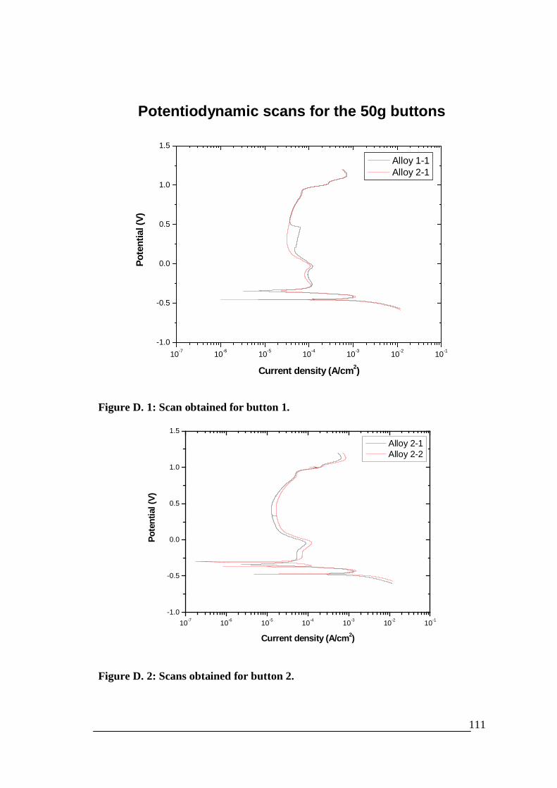
111
Potentiodynamic scans for the 50g buttons
10-7 10-6 10-5 10-4 10-3 10-2 10-1-1.0
-0.5
0.0
0.5
1.0
1.5
Pote
ntia
l (V)
Current density (A/cm2)
Alloy 1-1 Alloy 2-1
Figure D. 1: Scan obtained for button 1.
10-7 10-6 10-5 10-4 10-3 10-2 10-1-1.0
-0.5
0.0
0.5
1.0
1.5
Pote
ntia
l (V)
Current density (A/cm2)
Alloy 2-1 Alloy 2-2
Figure D. 2: Scans obtained for button 2.
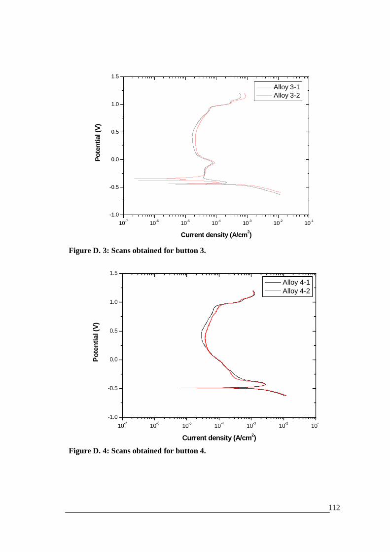
112
10-7 10-6 10-5 10-4 10-3 10-2 10-1
-1.0
-0.5
0.0
0.5
1.0
1.5
Pote
ntia
l (V)
Current density (A/cm2)
Alloy 3-1 Alloy 3-2
Figure D. 3: Scans obtained for button 3.
10-7 10-6 10-5 10-4 10-3 10-2 10-1-1.0
-0.5
0.0
0.5
1.0
1.5
Pote
ntia
l (V)
Current density (A/cm2)
Alloy 4-1 Alloy 4-2
Figure D. 4: Scans obtained for button 4.
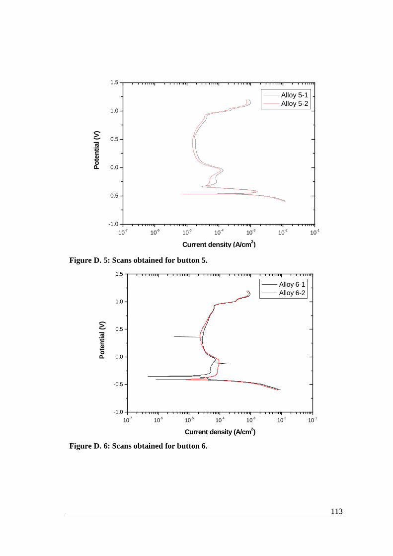
113
10-7 10-6 10-5 10-4 10-3 10-2 10-1
-1.0
-0.5
0.0
0.5
1.0
1.5
Pote
ntia
l (V)
Current density (A/cm2)
Alloy 5-1 Alloy 5-2
Figure D. 5: Scans obtained for button 5.
10-7 10-6 10-5 10-4 10-3 10-2 10-1-1.0
-0.5
0.0
0.5
1.0
1.5
Pote
ntia
l (V)
Current density (A/cm2)
Alloy 6-1 Alloy 6-2
Figure D. 6: Scans obtained for button 6.

114
10-7 10-6 10-5 10-4 10-3 10-2 10-1
-1.0
-0.5
0.0
0.5
1.0
1.5
Pote
ntia
l (V)
Current density (A/cm2)
Alloy 7-1 Alloy 7-2
Figure D. 7: Scans obtained for button 7.
10-7 10-6 10-5 10-4 10-3 10-2 10-1
-0.8
-0.6
-0.4
-0.2
0.0
0.2
0.4
0.6
0.8
1.0
1.2
1.4
Pote
ntia
l (V)
Current density (A/cm2)
Alloy 8-1 Alloy 8-2
Figure D. 8: Scans obtained for button 8.

115
10-7 10-6 10-5 10-4 10-3 10-2 10-1
-1.0
-0.5
0.0
0.5
1.0
1.5
Pote
ntia
l (V)
Current density (A/cm2)
Alloy 9-1 Alloy 9-2
Figure D. 9: Scans obtained for button 9.
10-7 10-6 10-5 10-4 10-3 10-2 10-1
-1.0
-0.5
0.0
0.5
1.0
1.5
Pote
ntia
l (V)
Current density (A/cm2)
Alloy 10-1 Alloy 10-2
Figure D. 10: Scans obtained for button 10.

116
10-7 10-6 10-5 10-4 10-3 10-2 10-1
-1.0
-0.5
0.0
0.5
1.0
1.5
Pote
ntia
l (V)
Current density (A/cm2)
Alloy 11-1 Alloy 11-2
Figure D. 11: Scans obtained for button 11.
10-7 10-6 10-5 10-4 10-3 10-2 10-1-1.0
-0.5
0.0
0.5
1.0
1.5
Pote
ntia
l (V)
Current density (A/cm2)
Alloy 12-1 Alloy 12-2
Figure D. 12: Scans obtained for button 12.
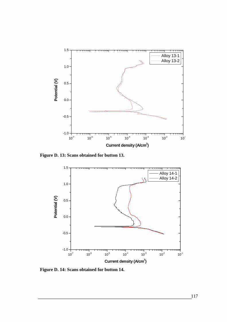
117
10-7 10-6 10-5 10-4 10-3 10-2 10-1-1.0
-0.5
0.0
0.5
1.0
1.5
Pote
ntia
l (V)
Current density (A/cm2)
Alloy 13-1 Alloy 13-2
Figure D. 13: Scans obtained for button 13.
10-7 10-6 10-5 10-4 10-3 10-2 10-1
-1.0
-0.5
0.0
0.5
1.0
1.5
Pote
ntia
l (V)
Current density (A/cm2)
Alloy 14-1 Alloy 14-2
Figure D. 14: Scans obtained for button 14.
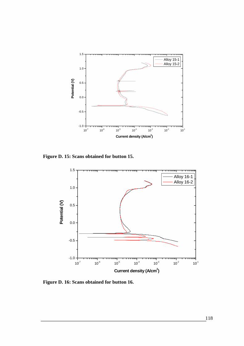
118
10-7 10-6 10-5 10-4 10-3 10-2 10-1-1.0
-0.5
0.0
0.5
1.0
1.5
Pote
ntia
l (V)
Current density (A/cm2)
Alloy 15-1 Alloy 15-2
Figure D. 15: Scans obtained for button 15.
10-7 10-6 10-5 10-4 10-3 10-2 10-1
-1.0
-0.5
0.0
0.5
1.0
1.5
Pote
ntia
l (V)
Current density (A/cm2)
Alloy 16-1 Alloy 16-2
Figure D. 16: Scans obtained for button 16.
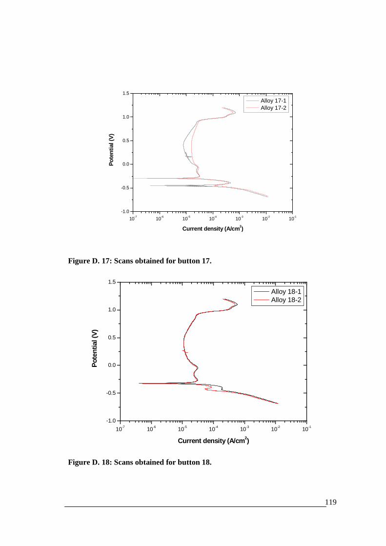
119
10-7 10-6 10-5 10-4 10-3 10-2 10-1
-1.0
-0.5
0.0
0.5
1.0
1.5
Pote
ntia
l (V)
Current density (A/cm2)
Alloy 17-1 Alloy 17-2
Figure D. 17: Scans obtained for button 17.
10-7 10-6 10-5 10-4 10-3 10-2 10-1
-1.0
-0.5
0.0
0.5
1.0
1.5
Pote
ntia
l (V)
Current density (A/cm2)
Alloy 18-1 Alloy 18-2
Figure D. 18: Scans obtained for button 18.

120
Appendix E: Results of potentiodynamic scansobtained for the ingots.
Table E. 1: Corrosion results for the 5 kg ingots.
alloycorrosion rate
(mm/y) icorr(A/m2) ipass (A/m2) icrit (A/m2)1 9.47 8.89 0.01 4.452 12.71 11.92 0.01 5.963 0.30 0.28 0.01 0.144 11.61 10.93 0.01 5.475 7.16 6.73 0.01 3.376 5.61 5.21 0.05 2.637 0.29 0.27 0.02 0.148 5.64 5.29 0.01 2.659 0.22 0.21 0.01 0.1110 0.17 0.16 0.01 0.0811 0.17 0.15 0.01 0.0812 0.16 0.14 0.01 0.0813 0.12 0.12 0.01 0.0714 0.11 0.12 0.01 0.0715 0.07 0.08 0.01 0.0416 0.10 0.11 0.01 0.0617 0.11 0.12 0.01 0.0618 0.05 0.05 0.01 0.03
*201 8.30 8.02 0.090 9.5*304 2.80 2.71 0.077 4.9*Herc 35.0 33.82 0.085 32
* Values for the reference alloys as cited in Mintek Communication C4105M[Moema and Papo, 2005, Mintek, pp. 54].
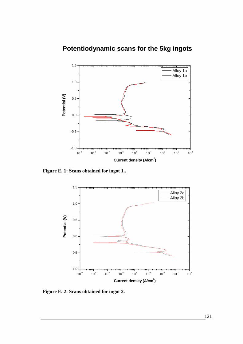
121
Potentiodynamic scans for the 5kg ingots
10-9 10-8 10-7 10-6 10-5 10-4 10-3 10-2 10-1-1.0
-0.5
0.0
0.5
1.0
1.5
Pote
ntia
l (V)
Current density (A/cm2)
Alloy 1a Alloy 1b
Figure E. 1: Scans obtained for ingot 1..
10-9 10-8 10-7 10-6 10-5 10-4 10-3 10-2 10-1-1.0
-0.5
0.0
0.5
1.0
1.5
Pote
ntia
l (V)
Current density (A/cm2)
Alloy 2a Alloy 2b
Figure E. 2: Scans obtained for ingot 2.
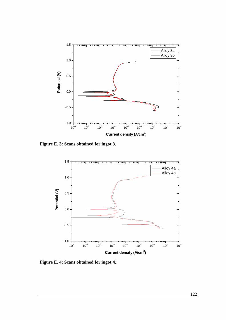
122
10-9 10-8 10-7 10-6 10-5 10-4 10-3 10-2 10-1-1.0
-0.5
0.0
0.5
1.0
1.5
Pote
ntia
l (V)
Current density (A/cm2)
Alloy 3a Alloy 3b
Figure E. 3: Scans obtained for ingot 3.
10-9 10-8 10-7 10-6 10-5 10-4 10-3 10-2 10-1-1.0
-0.5
0.0
0.5
1.0
1.5
Pote
ntia
l (V)
Current density (A/cm2)
Alloy 4a Alloy 4b
Figure E. 4: Scans obtained for ingot 4.

123
10-9 10-8 10-7 10-6 10-5 10-4 10-3 10-2 10-1
-0.8
-0.6
-0.4
-0.2
0.0
0.2
0.4
0.6
0.8
1.0
1.2
Pote
ntia
l (V)
Current density (A/cm2)
Alloy 5a Alloy 5b
Figure E. 5: Scans obtained for ingot 5.
10-9 10-8 10-7 10-6 10-5 10-4 10-3 10-2 10-1
-1.0
-0.5
0.0
0.5
1.0
1.5
Pote
ntia
l (V)
Current density (A/cm2)
Alloy 6a Alloy 6b
Figure E. 6: Scans obtained for ingot 6.

124
10-9 10-8 10-7 10-6 10-5 10-4 10-3 10-2 10-1-1.0
-0.5
0.0
0.5
1.0
1.5
Pote
ntia
l (V)
Current density (A/cm2)
Alloy 7a Alloy 7b
Figure E. 7: Scans obtained for ingot 7.
10-10 10-9 10-8 10-7 10-6 10-5 10-4 10-3 10-2 10-1-1.0
-0.5
0.0
0.5
1.0
1.5
Pote
ntia
l (V)
Current density (A/cm2)
Alloy 8a Alloy 8b
Figure E. 8: scans obtained for ingot 8.
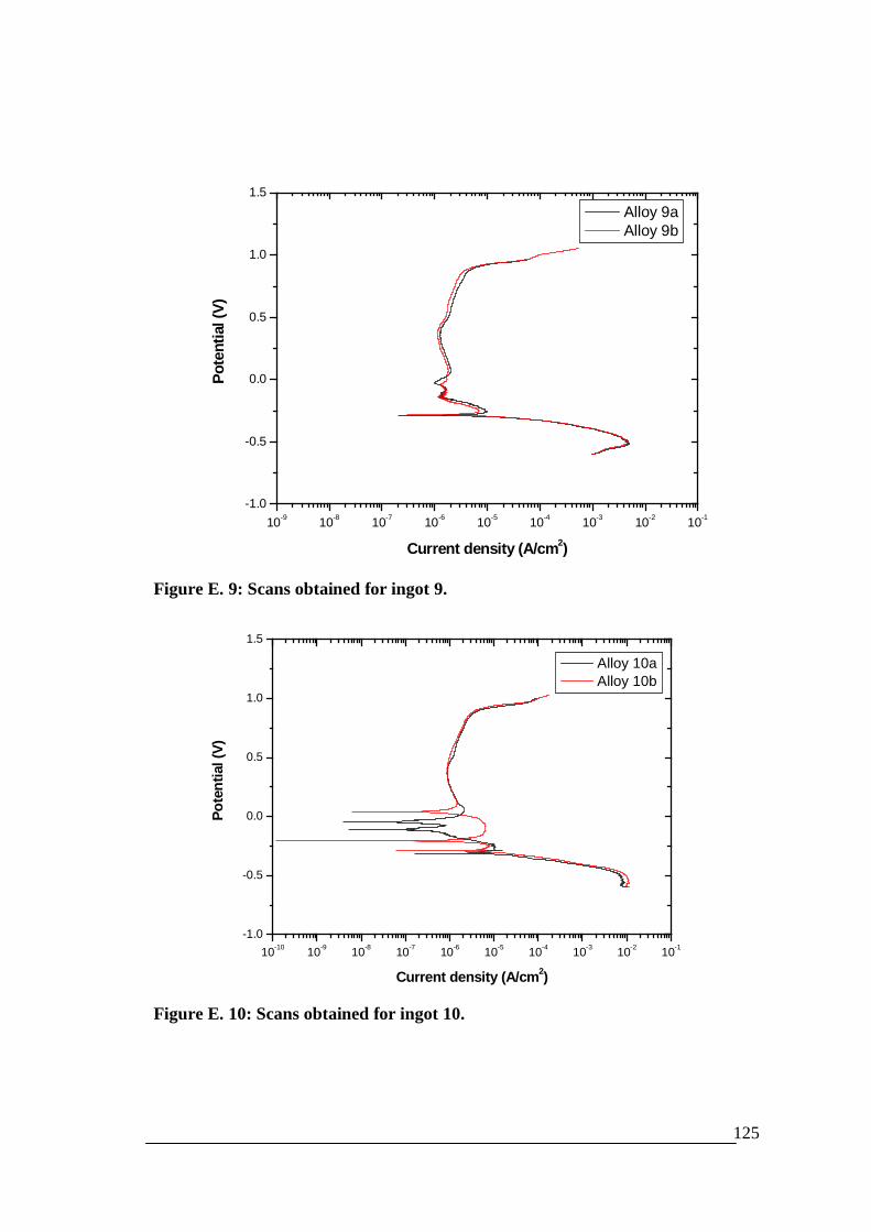
125
10-9 10-8 10-7 10-6 10-5 10-4 10-3 10-2 10-1-1.0
-0.5
0.0
0.5
1.0
1.5
Pote
ntia
l (V)
Current density (A/cm2)
Alloy 9a Alloy 9b
Figure E. 9: Scans obtained for ingot 9.
10-10 10-9 10-8 10-7 10-6 10-5 10-4 10-3 10-2 10-1-1.0
-0.5
0.0
0.5
1.0
1.5
Pote
ntia
l (V)
Current density (A/cm2)
Alloy 10a Alloy 10b
Figure E. 10: Scans obtained for ingot 10.
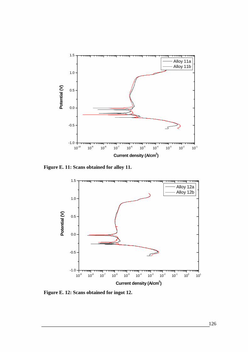
126
10-10 10-9 10-8 10-7 10-6 10-5 10-4 10-3 10-2 10-1-1.0
-0.5
0.0
0.5
1.0
1.5
Pote
ntia
l (V)
Current density (A/cm2)
Alloy 11a Alloy 11b
Figure E. 11: Scans obtained for alloy 11.
10-9 10-8 10-7 10-6 10-5 10-4 10-3 10-2 10-1 100 101
-1.0
-0.5
0.0
0.5
1.0
1.5
Pote
ntia
l (V)
Current density (A/cm2)
Alloy 12a Alloy 12b
Figure E. 12: Scans obtained for ingot 12.
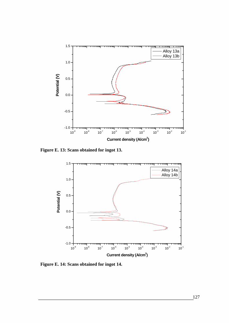
127
10-9 10-8 10-7 10-6 10-5 10-4 10-3 10-2 10-1-1.0
-0.5
0.0
0.5
1.0
1.5
Pote
ntia
l (V)
Current density (A/cm2)
Alloy 13a Alloy 13b
Figure E. 13: Scans obtained for ingot 13.
10-9 10-8 10-7 10-6 10-5 10-4 10-3 10-2 10-1-1.0
-0.5
0.0
0.5
1.0
1.5
Pote
ntia
l (V)
Current density (A/cm2)
Alloy 14a Alloy 14b
Figure E. 14: Scans obtained for ingot 14.
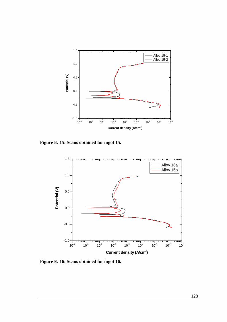
128
10-9 10-8 10-7 10-6 10-5 10-4 10-3 10-2 10-1-1.0
-0.5
0.0
0.5
1.0
1.5
Pote
ntia
l (V)
Current density (A/cm2)
Alloy 15-1 Alloy 15-2
Figure E. 15: Scans obtained for ingot 15.
10-9 10-8 10-7 10-6 10-5 10-4 10-3 10-2 10-1
-1.0
-0.5
0.0
0.5
1.0
1.5
Pote
ntia
l (V)
Current density (A/cm2)
Alloy 16a Alloy 16b
Figure E. 16: Scans obtained for ingot 16.
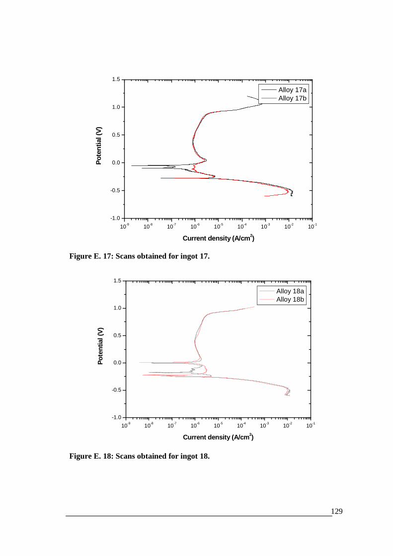
129
10-9 10-8 10-7 10-6 10-5 10-4 10-3 10-2 10-1
-1.0
-0.5
0.0
0.5
1.0
1.5
Pote
ntia
l (V)
Current density (A/cm2)
Alloy 17a Alloy 17b
Figure E. 17: Scans obtained for ingot 17.
10-9 10-8 10-7 10-6 10-5 10-4 10-3 10-2 10-1-1.0
-0.5
0.0
0.5
1.0
1.5
Pote
ntia
l (V)
Current density (A/cm2)
Alloy 18a Alloy 18b
Figure E. 18: Scans obtained for ingot 18.
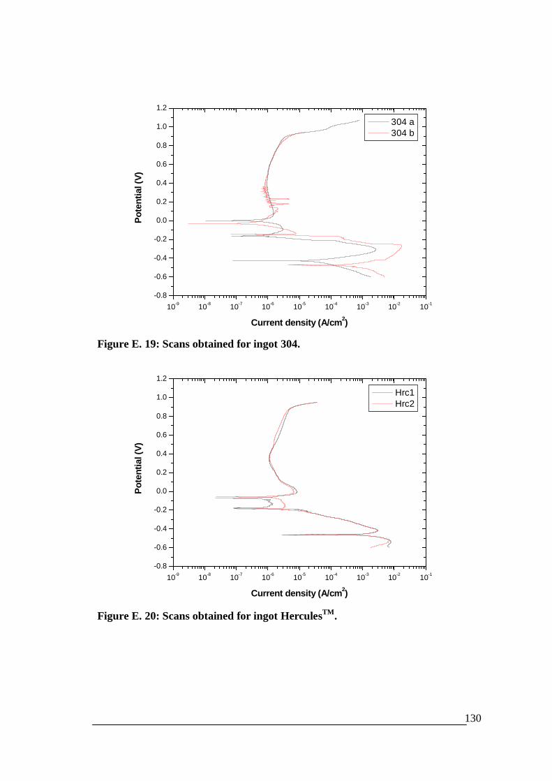
130
10-9 10-8 10-7 10-6 10-5 10-4 10-3 10-2 10-1-0.8
-0.6
-0.4
-0.2
0.0
0.2
0.4
0.6
0.8
1.0
1.2
Pote
ntia
l (V)
Current density (A/cm2)
304 a 304 b
Figure E. 19: Scans obtained for ingot 304.
10-9 10-8 10-7 10-6 10-5 10-4 10-3 10-2 10-1-0.8
-0.6
-0.4
-0.2
0.0
0.2
0.4
0.6
0.8
1.0
1.2
Pote
ntia
l (V)
Current density (A/cm2)
Hrc1 Hrc2
Figure E. 20: Scans obtained for ingot HerculesTM.
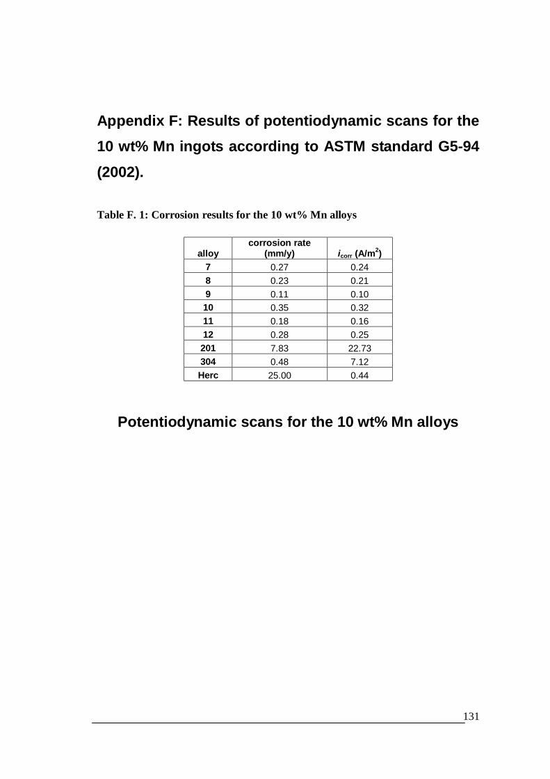
131
Appendix F: Results of potentiodynamic scans for the10 wt% Mn ingots according to ASTM standard G5-94(2002).
Table F. 1: Corrosion results for the 10 wt% Mn alloys
alloycorrosion rate
(mm/y) icorr (A/m2)7 0.27 0.248 0.23 0.219 0.11 0.1010 0.35 0.3211 0.18 0.1612 0.28 0.25
201 7.83 22.73304 0.48 7.12Herc 25.00 0.44
Potentiodynamic scans for the 10 wt% Mn alloys

132
10-5 10-4 10-3 10-2 10-1 100 101 102-800
-600
-400
-200
0
200
400
600
800
1000
1200
Pote
ntia
l (m
V)
Curret density (mA/cm2)
Ingot 7A Ingot 7B
Figure F. 1: Scans obtained for ingot 7.
10-5 10-4 10-3 10-2 10-1 100 101 102
-800
-600
-400
-200
0
200
400
600
800
1000
1200
Pote
ntia
l (m
V)
Current density (mA/cm2)
Alloy 8a Alloy 8b
Figure F. 2: Scans obtained for ingot 8.
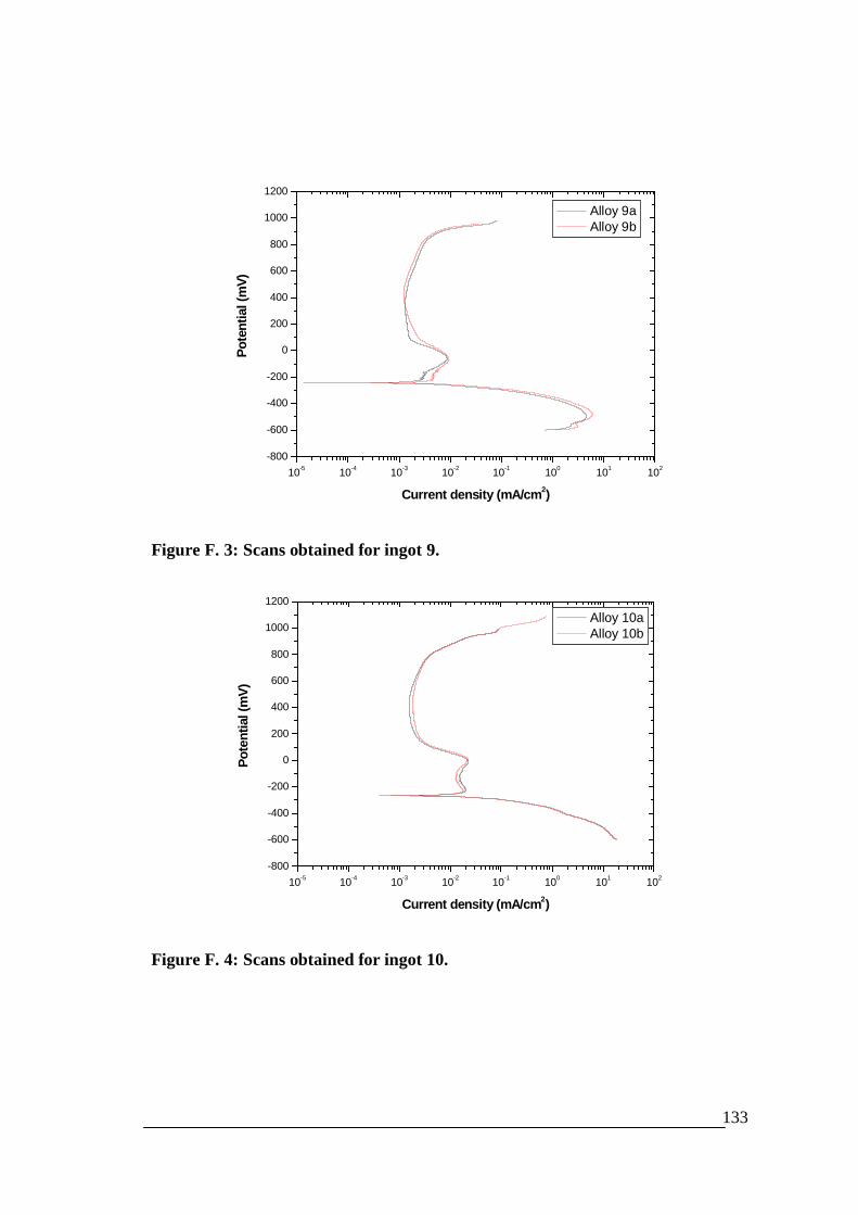
133
10-5 10-4 10-3 10-2 10-1 100 101 102
-800
-600
-400
-200
0
200
400
600
800
1000
1200
Pote
ntia
l (m
V)
Current density (mA/cm2)
Alloy 9a Alloy 9b
Figure F. 3: Scans obtained for ingot 9.
10-5 10-4 10-3 10-2 10-1 100 101 102
-800
-600
-400
-200
0
200
400
600
800
1000
1200
Pote
ntia
l (m
V)
Current density (mA/cm2)
Alloy 10a Alloy 10b
Figure F. 4: Scans obtained for ingot 10.
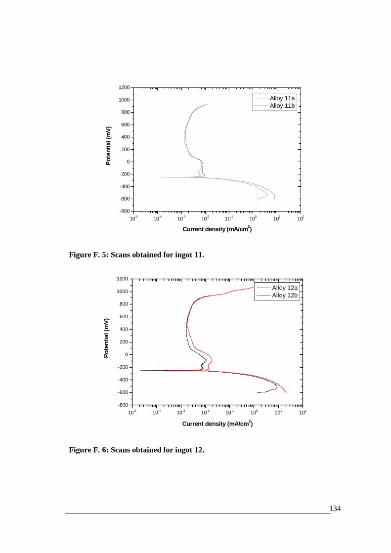
134
10-5 10-4 10-3 10-2 10-1 100 101 102-800
-600
-400
-200
0
200
400
600
800
1000
1200
Pote
ntia
l (m
V)
Current density (mA/cm2)
Alloy 11a Alloy 11b
Figure F. 5: Scans obtained for ingot 11.
10-5 10-4 10-3 10-2 10-1 100 101 102
-800
-600
-400
-200
0
200
400
600
800
1000
1200
Pote
ntia
l (m
V)
Current density (mA/cm2)
Alloy 12a Alloy 12b
Figure F. 6: Scans obtained for ingot 12.
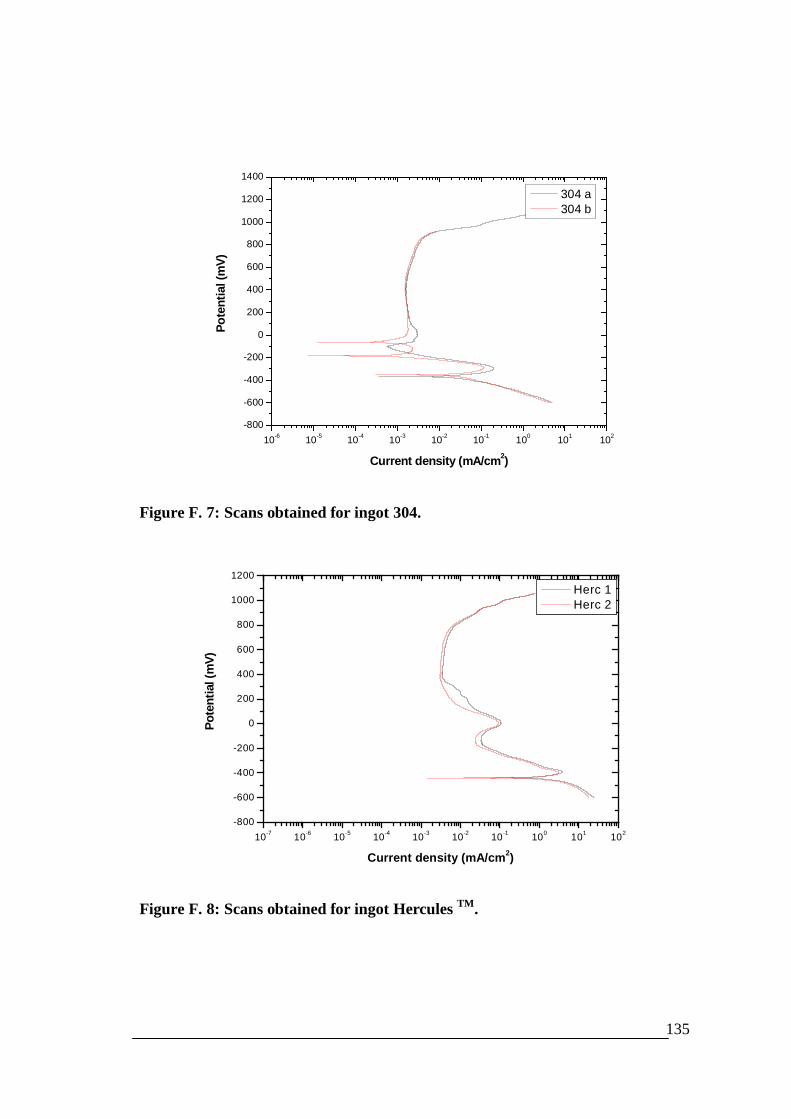
135
10-6 10-5 10-4 10-3 10-2 10-1 100 101 102-800
-600
-400
-200
0
200
400
600
800
1000
1200
1400
Pote
ntia
l (m
V)
Current density (mA/cm2)
304 a 304 b
Figure F. 7: Scans obtained for ingot 304.
10-7 10-6 10-5 10-4 10-3 10-2 10-1 100 101 102-800
-600
-400
-200
0
200
400
600
800
1000
1200
Pote
ntia
l (m
V)
Current density (mA/cm2)
Herc 1 Herc 2
Figure F. 8: Scans obtained for ingot Hercules TM.

136
10-7 10-6 10-5 10-4 10-3 10-2 10-1 100 101 102-800
-600
-400
-200
0
200
400
600
800
1000
1200
Pote
ntia
l (m
V)
Current density (mA/cm2)
201 a 201 b
Figure F. 9: Scans obtained for ingot 201.

137
Appendix G: Pitting corrosion results for 10 wt% Mningots.
Table G. 1: Pitting potentials for 10 wt% Mn alloys
alloy Epit(mV)7 36.058 96.779 132.7010 -7.2411 139.7812 233.41
201 28.06304 116.93herc -295.00
Pitting scans for the 10 wt% Mn alloys
10-7 10-6 10-5 10-4 10-3 10-2 10-1 100 101-500
-400
-300
-200
-100
0
100
200
300
400
Pote
ntia
l (m
V)
Current density (mA/cm2)
Pit 7a Pit 7b
Figure G. 1: Cyclic potentiodynamic scans for ingot 7.
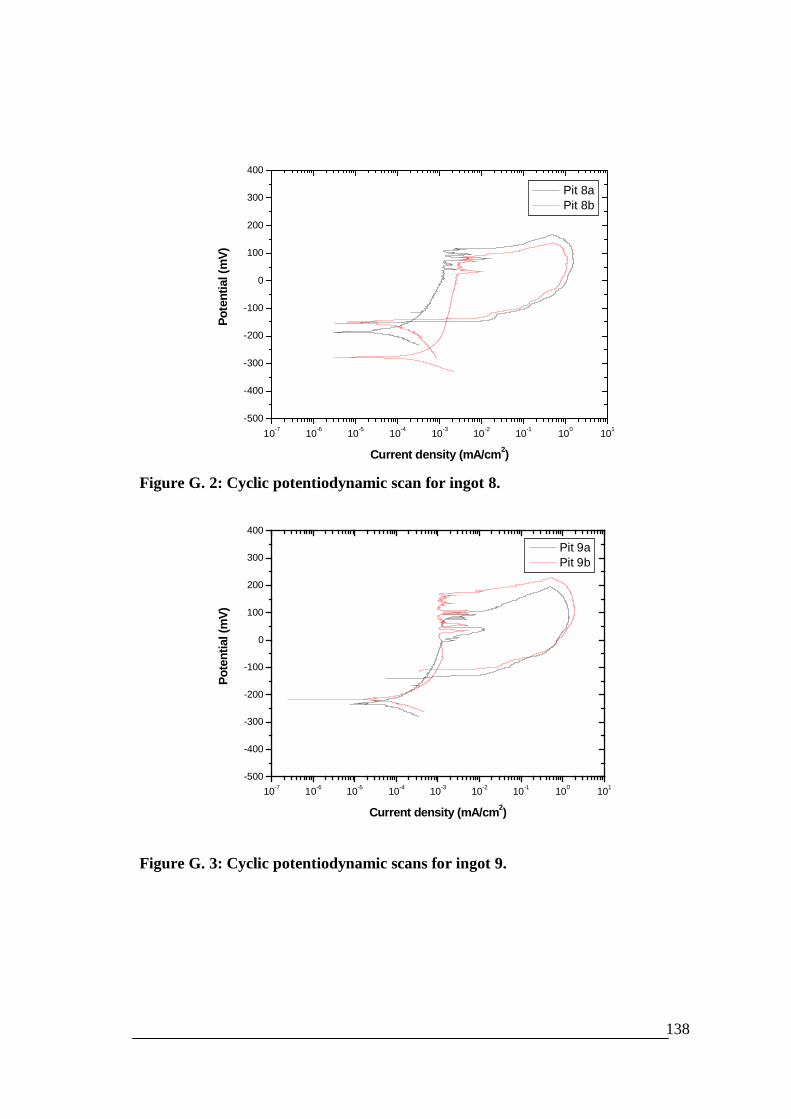
138
10-7 10-6 10-5 10-4 10-3 10-2 10-1 100 101-500
-400
-300
-200
-100
0
100
200
300
400
Pote
ntia
l (m
V)
Current density (mA/cm2)
Pit 8a Pit 8b
Figure G. 2: Cyclic potentiodynamic scan for ingot 8.
10-7 10-6 10-5 10-4 10-3 10-2 10-1 100 101-500
-400
-300
-200
-100
0
100
200
300
400
Pote
ntia
l (m
V)
Current density (mA/cm2)
Pit 9a Pit 9b
Figure G. 3: Cyclic potentiodynamic scans for ingot 9.

139
10-7 10-6 10-5 10-4 10-3 10-2 10-1 100 101-500
-400
-300
-200
-100
0
100
200
300
400
Pote
ntia
l (m
V)
Current density (mA/cm2)
Pit 10a Pit 10b
Figure G. 4: Cyclic potentiodynamic scans for ingot 10.
10-7 10-6 10-5 10-4 10-3 10-2 10-1 100 101-500
-400
-300
-200
-100
0
100
200
300
400
Pote
ntia
l (m
V)
Current density (mA/cm2)
Pit 11a Pit 11b
Figure G. 5: Cyclic potentiodynamic scans for ingot 11.
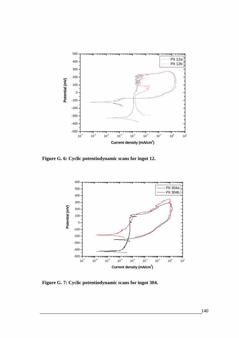
140
10-7 10-6 10-5 10-4 10-3 10-2 10-1 100 101-500
-400
-300
-200
-100
0
100
200
300
400
500
Pote
ntia
l (m
V)
Current density (mA/cm2)
Pit 12a Pit 12b
Figure G. 6: Cyclic potentiodynamic scans for ingot 12.
10-7 10-6 10-5 10-4 10-3 10-2 10-1 100 101-500
-400
-300
-200
-100
0
100
200
300
400
500
600
Pote
ntia
l (m
V)
Current density (mA/cm2)
Pit 304a Pit 304b
Figure G. 7: Cyclic potentiodynamic scans for ingot 304.
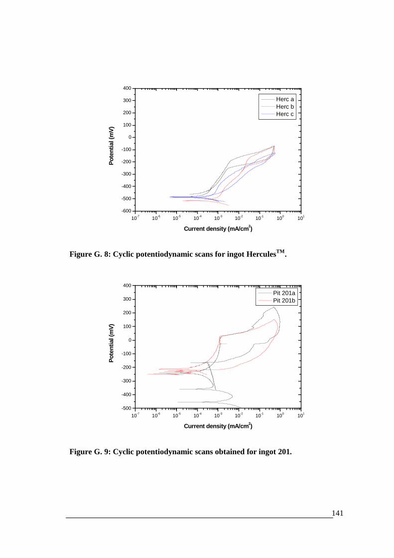
141
10-7 10-6 10-5 10-4 10-3 10-2 10-1 100 101-600
-500
-400
-300
-200
-100
0
100
200
300
400
Pote
ntia
l (m
V)
Current density (mA/cm2)
Herc a Herc b Herc c
Figure G. 8: Cyclic potentiodynamic scans for ingot HerculesTM.
10-7 10-6 10-5 10-4 10-3 10-2 10-1 100 101-500
-400
-300
-200
-100
0
100
200
300
400
Pote
ntia
l (m
V)
Current density (mA/cm2)
Pit 201a Pit 201b
Figure G. 9: Cyclic potentiodynamic scans obtained for ingot 201.
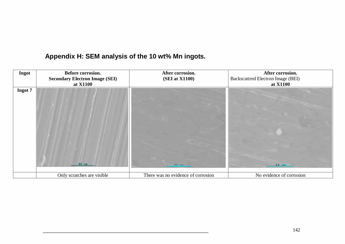
142
Appendix H: SEM analysis of the 10 wt% Mn ingots.
Ingot Before corrosion.Secondary Electron Image (SEI)
at X1100
After corrosion.(SEI at X1100)
After corrosion.Backscattred Electron Image (BEI)
at X1100Ingot 7
Only scratches are visible There was no evidence of corrosion No evidence of corrosion
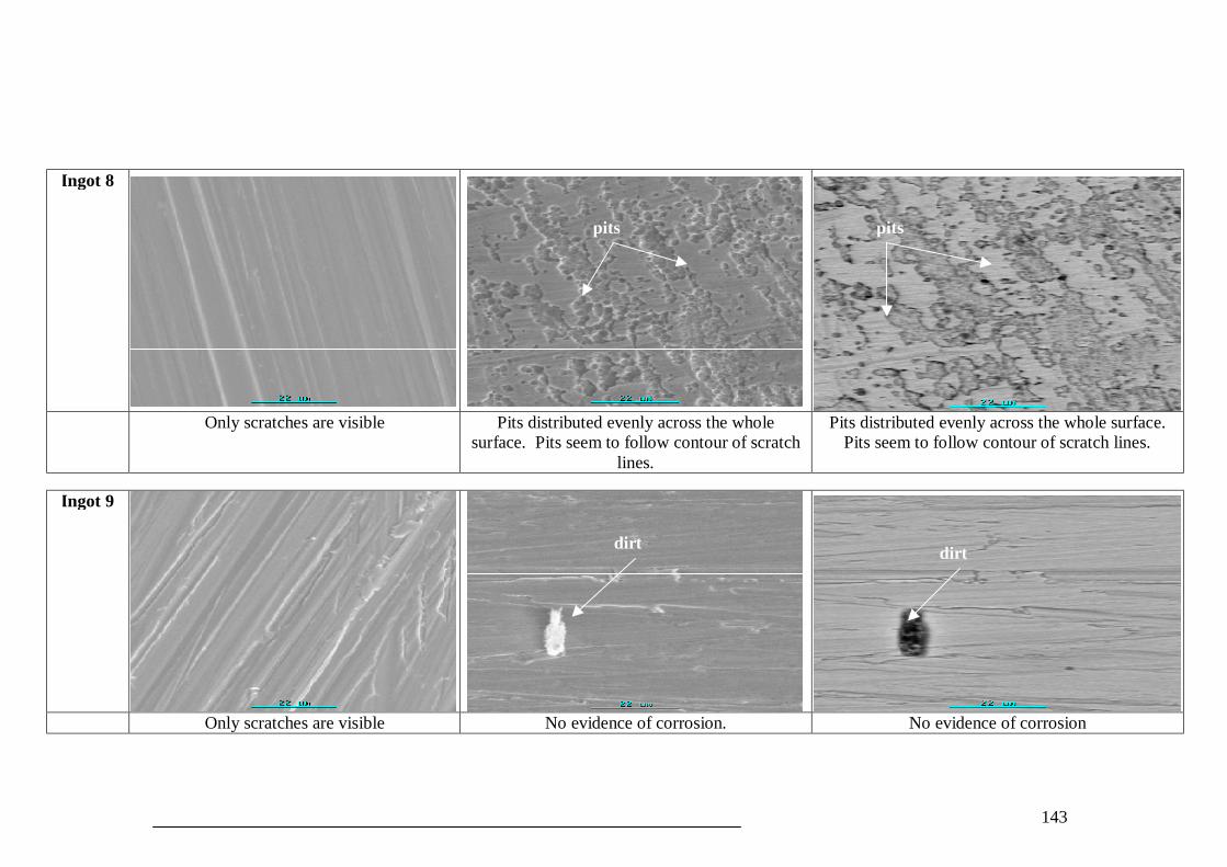
143
Ingot 8
Only scratches are visible Pits distributed evenly across the wholesurface. Pits seem to follow contour of scratch
lines.
Pits distributed evenly across the whole surface.Pits seem to follow contour of scratch lines.
Ingot 9
Only scratches are visible No evidence of corrosion. No evidence of corrosion
pits pits
dirt dirt
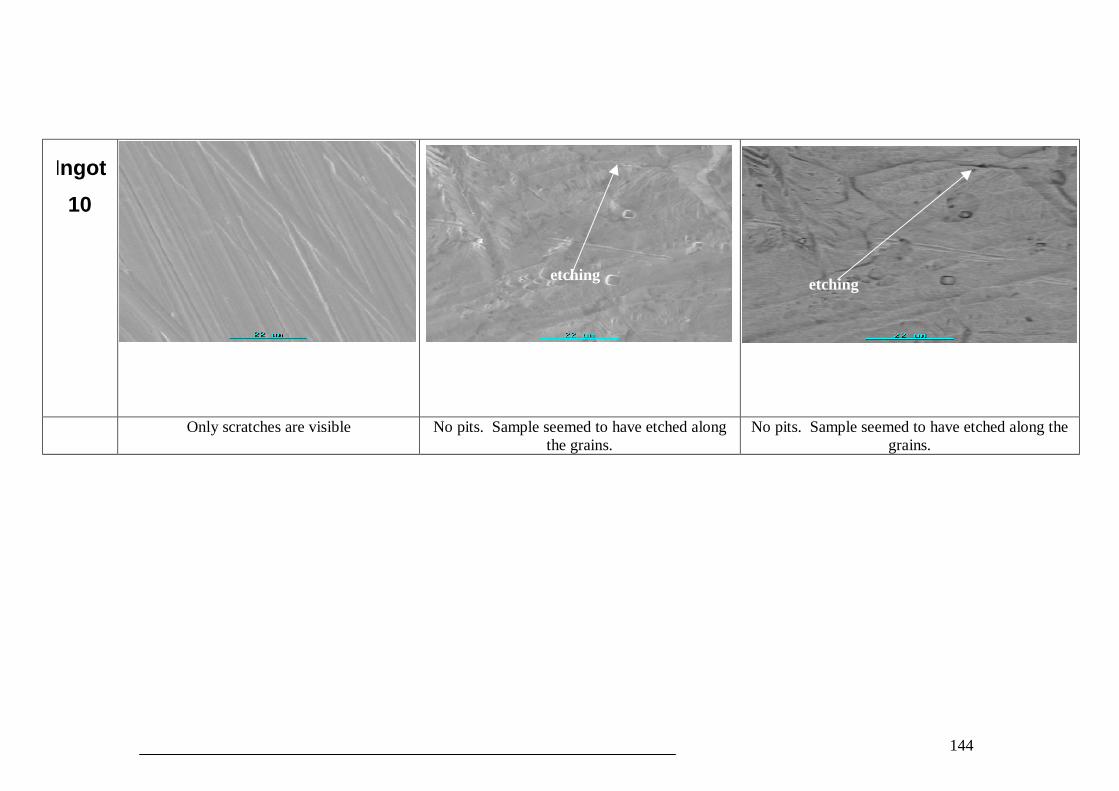
144
Ingot10
Only scratches are visible No pits. Sample seemed to have etched alongthe grains.
No pits. Sample seemed to have etched along thegrains.
etching etching
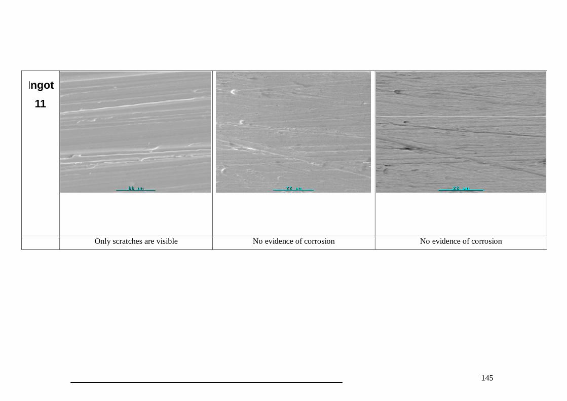
145
Ingot11
Only scratches are visible No evidence of corrosion No evidence of corrosion
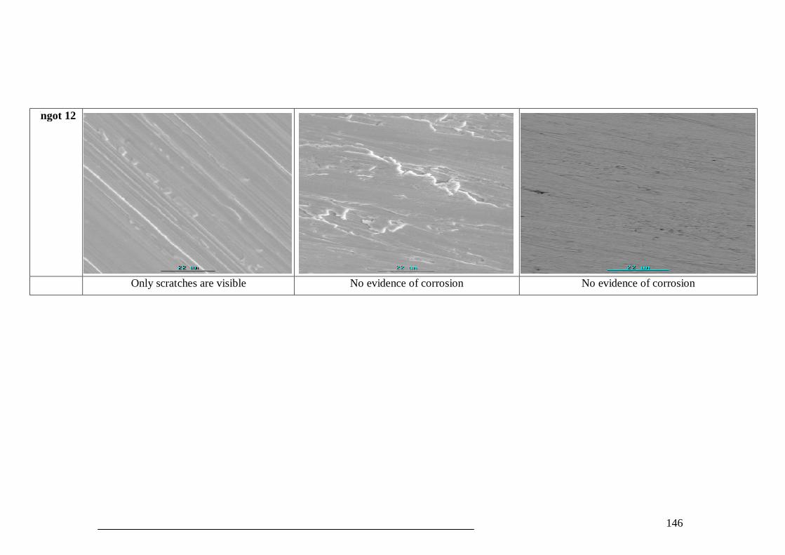
146
Ingot 12
Only scratches are visible No evidence of corrosion No evidence of corrosion
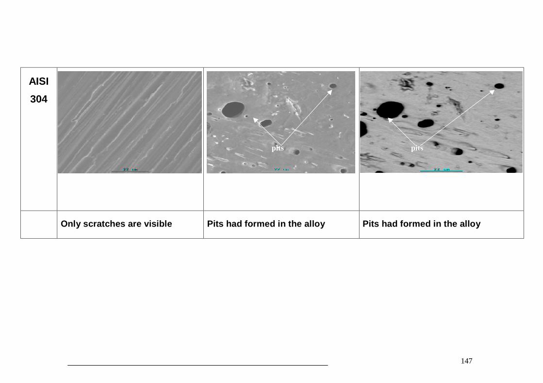
147
AISI304
Only scratches are visible Pits had formed in the alloy Pits had formed in the alloy
pits pits
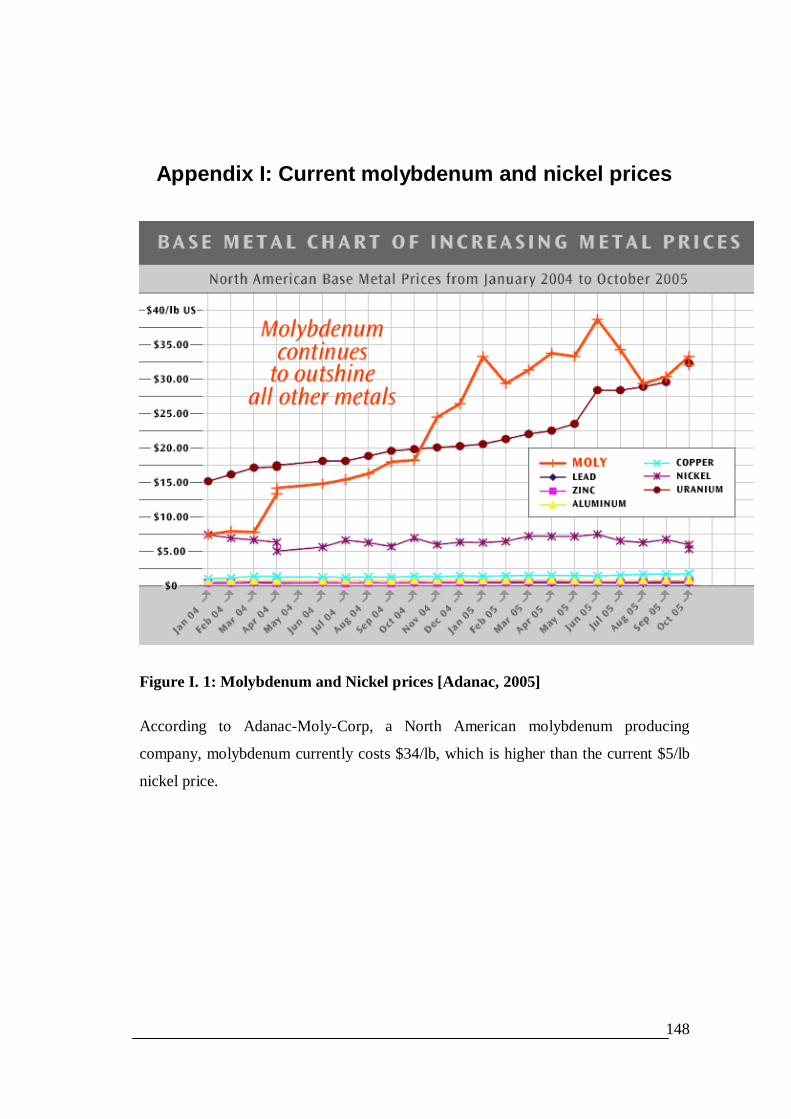
148
Appendix I: Current molybdenum and nickel prices
Figure I. 1: Molybdenum and Nickel prices [Adanac, 2005]
According to Adanac-Moly-Corp, a North American molybdenum producing
company, molybdenum currently costs $34/lb, which is higher than the current $5/lb
nickel price.