1

The Effect of Large-scale Performance-Based Funding in Higher Education Jason Ward a and Ben Ost a

a Department of Economics, University of Illinois at Chicago, 601 South Morgan UH718 M/C144 Chicago, IL 60607, United States Abstract: The use of performance-based funding that ties state higher education appropriations to performance metrics has increased dramatically in recent years, but most programs place a small percent of overall funding at stake. We analyze the effect of two notable exceptions—Ohio and Tennessee—where nearly all state funding is tied to performance measures. Using a difference-in-differences identification strategy along with a synthetic control approach, we find no evidence that these programs improve key academic outcomes. JEL Classification: I23 Keywords: Performance-based funding; Higher education

2

Introduction

In the United States, educational funding has historically been a function of inputs. K-12

teachers are typically paid based on years of experience and their certification (regardless of the

performance of their students). Public universities receive state funding based on the number of

students enrolled (regardless of the performance of those students). In the past decade, a

structural shift in funding mechanisms has taken hold at every level of education. From 2009 to

2015, the number of states requiring that teachers be evaluated based on student performance

tripled. Large school districts throughout the country have adopted new compensation systems

that directly link pay to performance (e.g., Dallas and Washington, DC). At the higher education

level, 10 states were in the process of developing new performance-based funding policies in

2015 alone (Snyder 2015). The shift to funding institutions based on outputs has affected every

level of education and it is expected to continue (McLendon and Hearn 2013; Hess and Castle

2008; Dee and Wyckoff 2015).

In this study, we provide the first evidence on the efficacy of a new set of higher

education performance-based funding policies implemented by Ohio and Tennessee in 2010 and

2011 respectively. These policies represent a dramatic shift in the scale of state funding

allocated based on performance, as well as the nature of the incentivized outcomes. In terms of

funding at stake, Tennessee now allocates over 80% of total state dollars using their outcomes

formula and Ohio allocates 100% (Synder 2016). In terms of outcome measures, these programs

both shift away from course completion counts to incentivize persistence and degree completion

amongst enrolled students.

3

Performance-based funding for higher education has existed since the late 1970s but early

programs were limited in scope. Starting in the 2000s, a series of states introduced more

consequential performance-based funding measures. This series of policy reforms has been

dubbed “PBF 2.0” to distinguish them from PBF 1.0 policies, which typically offered low

amounts of funding in the form of bonuses and did not tie this funding to outcomes such as

graduation rates (McLendon et al. 2006). PBF 2.0 policies placed larger amounts of funding at

stake (between 2% and 10%) and, while this funding was still often in the form of bonuses, some

states began to place baseline funding at risk as well. Additionally, this second wave of programs

began to tie funding more directly to outcome metrics such as credit hour accumulation and

graduation rates. The literature has generally found PBF 1.0 to have had little (or sometimes

negative) effects, a finding attributed to the fact that PBF 1.0 had limited scope and poor

implementation (Layzell 1999; Dougherty and Reddy 2011; Rutherford and Rabovsky 2014).

Despite having higher stakes and being better targeted, the literature to date has found

that PBF 2.0 also had limited impact on student performance (Hillman, Tandberg, and Gross

2014; Hillman, Tandberg, and Fryar 2015; Tandberg and Hillman 2014; Rutherford and

Rabovsky 2014). Recent performance-based funding programs enacted in Ohio and Tennessee

bear important similarities to PBF 2.0 programs in terms of allocating baseline funding on the

basis of incentivized outcomes, but they allocate all or nearly all base funding according to this

incentive structure. This large difference in stakes led Kelchen and Stedrak (2016) to dub these

programs PBF 3.0, a convention we follow in this work. To date, there is no evidence on the

effect of these policies on student outcomes.

Proponents of performance funding argue that the lack of efficacy of PBF 2.0 policies is

due to their limited scope – not because performance-based funding is generally ineffective.

4

Many states appear to be persuaded by such arguments and are moving toward PBF 3.0 type

programs despite limited existing evidence that PBF 2.0 has been effective and no existing

evidence on the efficacy of PBF 3.0 (Snyder 2015). Our study contributes to the literature by

providing the first estimates on the efficacy of PBF 3.0 policies. Estimating the efficacy of these

full-scale PBF programs will help state policy makers assess whether PBF 2.0 policies are

ineffective because of their small scope and misaligned incentives, or whether performance

funding is more generally ineffective at the higher education level.

We examine the effect of high-stakes performance-based funding on several different

academic outcomes. First, we examine total degree completions, as this outcome is directly

incentivized by performance-based funding. Second, we measure three dimensions of

undergraduate success: first-to-second-year retention, six-year graduation rates, and total BA

completions.1, 2 Though first-to-second year retention and six-year graduation rates are common

measures of institutional performance, one limitation of these measures is that they are only

defined for first-time, full-time freshman. The total BA completions outcome represents a

broader class of students. We use multiple measures of undergraduate success because there are

many different policy objectives in higher education and the outcome of interest depends on the

policy objective. First-to-second year retention and six-year graduation rates are key metrics for

students considering whether to enroll in a particular university. Total degree completions and

1 As we discuss in the institutional background section, some of the outcomes are directly incentivized, while others are not. Our goal is to assess how PBF affects core academic outcomes whether they are directly incentivized or not. 2 Our analysis focuses on undergraduates at four-year schools, so we do not consider associate degree production. Community colleges are also subject to performance-based funding and, though several papers examine the effect of early PBF programs on community colleges, there is no evidence on the effect of high-stakes PBF on community colleges. We view this as a useful direction for future work.

5

BA completions are the relevant outcomes for policy makers interested in increasing the

proportion of the state that is college educated.

Using a difference-in-differences strategy, we find no evidence that PBF 3.0 affected

total degree completions, first-to-second year retention, six-year graduation rates or BA

completions. Though estimates are near zero for all four outcomes, the precision of the estimate

varies across outcomes, and we only have precise null estimates for first-to-second year retention

and six-year graduation rates. For total degree completions and BA completions, there is no

statistically significant evidence of improvement on either outcome, but standard errors are

sufficiently large so that moderate effects are included in the confidence intervals.

In order to assess the validity of the results, we estimate a dynamic difference-in-

differences model that includes leads and lags of the policy effect. Specifically, we examine

whether the policies have an “effect” on outcomes in the years leading up to implementation and

we directly assess whether there appears to be differential trends in treatment states vs control

states. In addition to paying careful attention to whether treatment and control trend similarly

prior to policy adoption, we complement the difference-in-differences analysis by implementing

a synthetic control approach (Abadie et al 2010). The synthetic control approach constructs a

weighted control group that minimizes pre-policy differences between the control group and the

treatment group and compares outcome trends in the post-adoption period.

In addition to assessing the overall effect of PBF 3.0 on academic outcomes, we consider

potential mechanisms through which institutions might attempt to improve outcomes. First, we

consider whether institutions alter overall spending or the proportion of spending that goes to

instruction, student supports or research. Second, we consider whether institutions enroll more

students or a different type of student in response to PBF 3.0. Enrolling more students can help

6

increase outcomes such as total degree production and altering student composition can help

increase graduation rates.3 We find little evidence of an institutional response on either the

institutional spending or student enrollment dimensions. The one exception is that we find that

the proportion of Hispanic students falls slightly following PBF 3.0. An important caveat to these

findings is that we cannot rule out moderate effects, since many of the coefficients are not

precisely estimated.

Our study makes three main contributions. First, as noted above, PBF 3.0 represents a

significant evolution of scope of performance-based funding policies and there is little reason to

expect that the literature evaluating small-scale performance-based funding would be informative

regarding the likely effects of full-fledged performance-based funding. Our study provides the

first evidence on the effect of PBF 3.0 on core academic outcomes. Second, we are the first study

to use a synthetic control approach to study the effect of PBF and among only a few studies that

empirically assess the plausibility of the parallel trend assumption when estimating difference-in-

differences models. Finally, our study provides a comprehensive analysis by examining multiple

performance measures along with student compositional changes and institutional spending,

outcomes that may shed light on institutional responses to PBF 3.0.

There are several limitations to our analysis. First, we only study the effect of the

Tennessee and Ohio policies and so our results may not generalize to other states where

implementation details and existing institutional contexts differ. The institutional context

surrounding higher education is very heterogeneous across states and so this is an important

limitation. Second, our analysis is limited to the six years after policy implementation and so we

3 In both Tennessee and Ohio, there are also explicit provisions in the policy that provide incentives to enroll traditionally underrepresented or disadvantaged students.

7

are only able to assess the short-run effect of PBF 3.0. This is a particularly important limitation

when considering outcomes such as six-year graduation rates. Third, our estimates are only

statistically precise for first-to-second year retention and six-year graduation so we cannot make

strong conclusions regarding degree completions. Finally, the difference-in-differences design

relies on a fundamentally untestable assumption that trends in the control group provide a valid

counterfactual for trends in the treatment group. We test this assumption indirectly by looking

for parallel trends in the pre-period, but we cannot definitively rule out that our estimates may be

affected by unobservable differential trends between “treated” states and the states we use for

comparison.

Literature Review

We focus here on discussing the quantitative literature that aims to estimate the effect of

PBF on academic outcomes at four-year institutions.4 We refer the reader to Dougherty and

Reddy (2011) for a comprehensive review of both the quantitative and qualitative literature on

the effect of performance-based funding on a variety of immediate, intermediate and ultimate

outcomes. We further restrict our analysis to studies that strive to identify the causal effect of

PBF and refer the reader to Tandberg and Hillman (2014) for a discussion of additional studies

that examine associations with PBF.

4 Hillman, Tandberg, and Fryar (2015) study community colleges in Washington state and Tandberg, Hillman and Barakat (2014) study community colleges nationally. We emphasize the literature studying four-year schools here because the policies, and institutional context surrounding four-year schools is quite different from that of community colleges. That said, it is important to emphasize that the two-year college sector is arguably just as important as the four-year college sector and future work should assess the effect of PBF 3.0 on two-year colleges.

8

Tandberg and Hillman (2014) estimate the causal effect of PBF on BA degree

completions among four-year institutions using a difference-in-differences approach, finding no

evidence of a non-zero effect. They note that further research could examine whether states with

stronger incentives generate different educational outcomes.” 5 Rutherford and Rabovsky (2014)

perform a similar national analysis taking advantage of the disparate timing of PBF adoption

across states. They examine whether PBF 1.0 and PBF 2.0 policies have different effects on

outcomes such as graduation rates and first-to-second year persistence. Their results show no

evidence of either PBF 1.0 or PBF 2.0 affecting academic outcomes. Neither of these studies

directly assess whether pre-trends are similar across treated and control states.

Hillman, Tandberg and Gross (2014) analyze the effect of a PBF policy enacted in

Pennsylvania in 2000 on BA completions. They use difference-in-differences and provide a

direct assessment of the whether treatment and control trended similar in the pre-policy period.

They find that control institutions defined by geographic proximity show evidence of differential

trends prior to the policy and use an approach matching Pennsylvania institutions to other

institutions based on 1990 characteristics to generate a control group that trended similarly to

Pennsylvania institutions prior to the 2000 policy. With this approach, they find no effect of the

PBF policy on BA degree production.6

Sanford and Hunter (2011) study the effects of earlier PBF policies in Tennessee on 6-

year graduation rates and first-to-second year retention rates. They utilize spline-linear mixed

5 Interestingly, in discussing how treatment intensity varies across states in their (pre-2011) data, Tandberg and Hillman point to the example of Pennsylvania which allocates 8% of appropriations to performance whereas Oklahoma allocates 2%. The PBF 3.0 reforms come too late to be included in their analysis. 6 Hillman, Tandberg and Gross note that one limitation of their study is that they only use a single outcome (BA production per 100 students) and it is possible that the Pennsylvania policy could have affected other important dimensions of institutional success

9

models and control for observable institutional characteristics and find no evidence that early

PBF programs in Tennessee were effective.

Conceptual framework

Performance-based funding is motivated by the idea that state funding of higher

education fits into a classical principal-agent framework. There are two key features of a

principal-agent model: asymmetric information and divergent preferences between the principal

and the agent. In this context, the principal (the state) seeks to improve student outcomes,

whereas the agents (university administrators) have a different objective. The principal can

observe final outcomes but is assumed to be unable to perfectly observe inputs. In a principal-

agent model, compensation schemes that fail to tie compensation to output will result in

inefficient outcomes from the principal’s perspective. This is the concern with traditional

funding models and a major reason that performance-based funding has grown in popularity.

In a traditional funding model, universities receive funding based on total enrollments

and administrators have little financial stake in the performance of those enrolled students. Such

a funding system may incentivize enrolling too many students, investing too little in improving

educational quality, or devoting resources to non-student outcomes. By tying funding to student

outcomes, the state changes the incentives of the university administrator and encourages them to

focus more resources on the incentivized outcomes. Whether or not this will be successful

depends on several factors.

First, incentivizing certain outcomes will only be effective if there was an initial

disconnect between the priorities of the state and the priorities of administrators. If the state

begins rewarding degree completions, but university administrators already strongly value

10

degree completions, the incentive may have no effect on behavior. Second, tying funding to

specific outcomes will only improve these outcomes if administrators have the knowledge and

ability to improve the incentivized outcomes. Improving outcomes such as degree completions is

a complex process and the institution’s administrator may have limited understanding of how to

improve these outcomes, even when she has a strong incentive to do so. Relatedly, in many

cases, institution administrators have limited autonomy and cannot experiment with new

approaches because of state-imposed regulations and requirements. Third, Holmstrom and

Milgrom (1991) note that performance pay has the potential to produce unintended consequences

when the agent has many different tasks to complete and only some of these tasks are directly

rewarded. Higher education institutions certainly have multiple outputs and, thus, the incentive

to increase certain outcomes may be at the expense of other outcomes. For example, institutions

focused primarily on increasing course and degree completions may reduce academic standards.

Dougherty et al. (2014) suggests that administrators intend to respond to the incentives of

performance-based funding and Dougherty and Reddy (2011) discuss various dimensions on

which institutions might alter inputs in an attempt to improve outcomes. Here we discuss four

broad dimensions that may allow administrators to affect outcomes. First, administrators can

expand a range of student services from academic counseling to academic supports such as

tutoring. Webber and Ehrenberg (2010) show that spending on student services increases

graduation rates, suggesting that institutions may have some capacity to improve outcomes

through these inputs. Second, administrators can devote more resources to instructional activities

such as providing more teaching assistants, reducing class sizes, or expanding incentives such as

awards and bonuses for exceptional teaching. Bettinger and Long (2018) find that smaller classes

improve student persistence and Philipp, Tretter and Rich (2016) find that undergraduate

11

teaching assistants help improve student class performance. Though there is little evidence on the

effect of teaching awards on student outcomes, Brawer et al. (2006) finds that faculty report

improving the quality of their teaching due to these awards.

Third, administrators could adopt data-driven approaches to student improvement by

introducing tracking systems that include predictive analytics to help better target interventions.

That said, there is mixed evidence on the efficacy of these types of data-driven approaches in

terms of actually improving student outcomes (Alamuddin, Rossman and Kurzweil 2018; Main

and Griffith 2018; Milliron, Malcom and Kil 2014). Finally, administrators could attempt to alter

the number and composition of entering students, either by altering recruiting efforts or by

explicitly changing admission requirements. This would likely have a direct effect on outcomes

through compositional change, and it may also have indirect effects on outcomes through a peer

effects channel.

Institutional Background

Our study is focused on the performance-based funding policies enacted by Ohio and

Tennessee in 2009 and 2010 respectively. Ohio and Tennessee were both early adopters of

performance-based funding, with Tennessee’s first program beginning in 1979 and Ohio’s first

program beginning in 1995. Both states provided universities with bonuses based on a variety of

performance measures, but neither had large amounts of funding at stake until the recent policy

changes. Importantly, in both states, the bonuses in the early programs were less than 5 percent

of state appropriations. Dougherty and Reddy (2011) provide a description of the qualitative

literature based on interviews with university administrators in Ohio and Tennessee. They find

that in both states, prior to 2010, performance funding was viewed as a trivial incentive given its

12

small scale. Nevertheless, rather than interpret our estimates as the effect of performance funding

relative to no performance funding, it is more appropriate to interpret our estimates as the effect

of moving from a very small performance funding program to a large-scale performance funding

program.

The recent policies enacted in Tennessee and Ohio represent a substantial shift in the

magnitude of performance-based funding. In Ohio, the funding reform moved all state higher

education funding to a formula-based allocation. In 2015, performance-based funding

determined around $4500 per full-time equivalent (FTE) student (Snyder 2015). Ohio’s initial

formula awarded points for accumulating credit hours (progression) at around 60%, for degree

completions at around 20%, and for Doctoral and medical degrees at around 20% (Ohio Higher

Ed Funding Commission, 2012).7 Performance-based funding in Tennessee—amounting to

around $4000 per FTE student—is determined similarly, but with greater weight on degree

production relative to Ohio’s initial formula, and with some weight on research and public

service.

Despite these differences in the details of implementation, the Ohio and Tennessee

programs are similar in their core design and implementation. Both programs convert multi-year

moving averages of an additive set of weighted measures—primarily consisting of counts of

students acquiring credit hours or completing a degree program—into points that determine what

proportion of the overall state instructional appropriation will accrue to a school.8 Both programs

include an incentive to increase admissions among disadvantaged students (e.g., low-income,

7 This formula was revised in 2014 and roughly inverted the relative weights for these two primary metrics. 8 In the first four years of the program Ohio used, variously, two- and five-year averages but standardized their program at three-year MAs in 2014, matching the averaging approach used in Tennessee.

13

adult students, underrepresented groups) that amounts to multipliers on these students in the

overall calculation of points for credit acquisition and graduation. Given the similarity of the

programs, our preferred analysis reduces noise by estimating the aggregate effect of these PBF

3.0 policies, but we also consider the programs separately. The pooled analysis provides an

estimate of the average effect across the two states and should be interpreted keeping in mind

that the programs are not identical.

In both Ohio and Tennessee, there was a short adjustment period to ensure that schools

would not lose too much funding in the first years of the program.9 Our empirical model assesses

the possibility that universities only respond to the policies once the stop-loss ended, but there

are several reasons that institutions had an incentive to respond earlier. First, institutions still had

an incentive to improve outcomes since it would be difficult to concentrate all of the

improvement in the year stop-loss ended. Second, although institutions were protected from large

losses during the stop-loss period, there was no cap on increased funding and so for many

schools, the stop-loss provision was moot. Finally, since performance is measured as a moving

average, outcomes during the stop-loss period still affected performance metrics in the later

periods. Though there are several reasons to expect a response during the stop-loss period, if

institutions expected that PBF would be eliminated before stop-loss ended, then we would expect

9 In Ohio, there was a formal stop-loss program for the first four years of the program that limited losses to a percentage of the prior year’s funding level. In FY 2011, changes were limited to 1%, FY2012, 2%, and FY2013, 3%. The state also included a final year of “bridge” funding in FY 2014 before transitioning to no stop loss. See the 2014 Performance-Based Funding Evaluation Report, available at https://www.ohiohighered.org/financial. Tennessee had no explicit stop-loss provision, but the funding adjustments necessary to transition to the performance-based funding model were phased in the during the first few years of the policy. (Personal Correspondence with Steven Gentile, Associate Chief Fiscal Officer of the Tennessee Higher Education Commission).

14

limited response in the early years of the program.

Though no other state has a performance-based funding policy that comes close to

matching the strength of the Ohio and Tennessee programs, many states have adopted smaller-

scale programs. This suggests that treating all states as controls could be inappropriate. That

said, it is unclear which states should be included in the control group because many states have

programs that put 0% of base funding at risk and do not reward persistence or graduation rates at

all. We follow the taxonomy developed by Snyder (2015) that classifies states into four

categories of performance funding. Our baseline control group consists of states with no

performance funding, but we also consider a control group that adds states that have

implemented only “rudimentary” performance funding.10 Rudimentary performance funding

programs do not link funding to college completion or cumulative attainment goals and only

include bonus funding (as opposed to putting baseline funding at risk).

Because we are interested in the effect of very high stakes performance funding, we

exclude states that had moderate performance-based funding from the analysis. These states have

not implemented the treatment of interest, but they are not an appropriate control group since

they have programs that place between 5 and 25 percent of funding at risk.

Data

Our primary source of data is the Integrated Postsecondary Education Data System

(IPEDS) that provides institution-level data for all schools that participate in Title IV funding.

We use IPEDS to measure total degree completions and three measures of undergraduate

10 Appendix table A1 lists the states in our main and restricted sample specifications.

15

success: first-to-second year retention, six-year graduation rates and BA completions.11 Total

degree completions is a measure of aggregate production and is directly incentivized by the

programs. First-to-second year retention provides a leading indicator of graduation rates and

improving this outcome is a priority for many institutions since the majority of attrition occurs

during the first few years. Six-year graduation rates are a standard measure of institutional

performance and capture an outcome that is critically important from the perspective of

individual students considering enrolling in a particular institution. BA completions capture a

broader class of students than graduation rates and is the outcome of interest for policy makers

interested in increasing the proportion of college-educated workers in a state. Though the four

outcomes are closely related, they need not move in lock-step and it is useful to consider all four

together.

We also use IPEDS data on full-time equivalent (FTE) enrollment, student composition

variables, and institutional spending in order to try to understand the mechanisms behind any

changes in outcomes. First, institutions could try to improve student outcomes by changing

spending patterns. We use IPEDS data on total institutional spending as well as the share

allocated to student supports, instructional spending and research spending. Second, institutions

may increase degree production by simply enrolling more students or enrolling a different type

of student. We measure total student enrollment, the proportion of undergraduates that are over

24, Pell dollars per enrolled student12, the proportion that are black, and the proportion that are

11 Total degrees captures the total number of BA, MA or Phd degrees granted by the institution in a given year. 12 Increases in Pell dollars per student could reflect increases in the proportion of students on Pell or it could reflect increases in the severity of need among the existing Pell recipients. It will not capture national changes in Pell grant generosity as all models include year fixed effects.

16

Hispanic. We supplement the IPEDS data with census data on time varying unemployment rates

and state demographics.

Table 1 shows descriptive statistics for 3 samples. Column (1) shows Ohio and Tennessee

(the treatment states), column (2) shows states that have no PBF programs during this time-

period (controls) and column (3) includes states that have at most rudimentary performance-

based funding during this period (alternative control group).13 Though the difference-in-

differences empirical approach does not require the treatment and control groups to have similar

characteristics in levels, examining the characteristics of treatment and control can be useful in

assessing external validity and may suggest areas of potential concern. Comparing across the 3

columns suggests that the treatment states are fairly similar to the control states in many, but not

all dimensions. Outcomes such as retention and graduation rates are similar across treatment and

control, but treatment institutions are generally larger and therefore generate more degrees per

year and have higher FTE enrollment. Treatment and control enroll a very similar type of student

in terms of Pell dollars per student and the proportion over 25, however, treated institutions

enroll far fewer Hispanic students compared to the control groups.

Table 2 shows descriptive statistics for our key academic outcomes before and after

policy adoption. Treatment states refer to Ohio and Tennessee and control states refer to states

that have no PBF programs. The alternative control group includes states that have, at most,

rudimentary performance-based funding during this period. The “difference” column for the

treatment states shows that treatment states experienced increased graduation rates, BA

completions and total degree completions over this time period. Though this pattern is

13 The “no-PBF” restriction generates a control group of 25 states. The less-restrictive “rudimentary PBF” restriction generates a control group of 34 states. The included states are detailed in Appendix Table A1.

17

encouraging, it may simply reflect national changes in higher education. Consistent with this

view, we see the same pattern of changes in these outcomes for the control states, regardless of

which control group we consider. For example, graduation rates increased by 3.16 percentage

points in the treatment states and by 3.6 percentage points in the control states. The raw

difference-in-differences are near zero for all four outcomes.

Though the simple difference-in-difference estimates are suggestive, Table 2 provides no

confidence intervals around these estimates and the point estimates could be contaminated by

pre-existing trends. In the following section, we describe our empirical model that places the

analysis in a more rigorous regression context.

Empirical Approach

Our empirical approach follows the related literature by estimating school-level

regressions that control for both school and year fixed effects (e.g. Kelchen and Stedrak 2016).

Specifically, for each outcome, we estimate the following two-way fixed effects regression

model

"#$ = & + ()*+,#$ + -.#$ + /# + 0$ + 1#$. (1)

*+,#$ is an indicator for whether a school is affected by performance-based funding 3.0 in a

particular year. We define this variable so that schools are considered affected by the policy

starting the year after the policy passes the state legislature. /# and 0$ are institution and year

fixed effects. "#$ is one of the 4 outcomes, and .#$ is a vector of time-varying characteristics

comprising the fraction of 18- to 26-year-olds in a state that are black or Hispanic, state

unemployment rates, interactions between these demographics and unemployment rates,

institutional total revenue and the share of revenue that comes from the state. In some

18

specifications, we also include baseline graduation rates interacted with a linear time trend. We

report analytic standard errors clustered at the state level, but results are very similar if we

bootstrap standard errors instead.

Equation (1) relies on the assumption that trends in the control states provide a valid

counterfactual for trends in the treatment states. Though this parallel trends assumption is

inherently untestable, we can provide suggestive evidence on its validity by re-estimating

equation (1) but providing the full event-study series of indicators for time relative to the policy

change. Specifically, we estimate

"#$ = & + ∑ (3453647 *+,#3 + ∑ (3

7368 *+,#3 + /# + 0$ + 1#$ (2)

Time period t-1 is the omitted category so all estimates are relative to the year before the policy

passes. If schools unaffected by the policy are trending differently than schools affected by the

policy, β-6 through β-2 will be trending up or down and this would cause us to doubt the validity

of our estimates from equation (1). In addition to providing a test of the validity of the empirical

design, the estimates of β0 through β6 in equation (2) provide an estimate of the time-path of the

policy effect.

To assess the importance of differential trends for our estimates, we also examine the

sensitivity of the estimates to the inclusion of state-specific linear time trends. If the difference-

in-differences assumption holds, estimates should be similar when state-specific time trends are

added to the model. Although the model with state-specific time trends allows for the possibility

of differential state trends, this model does not strictly dominate the simpler difference-in-

differences model because it requires the equally strong assumption that deviations from a linear

trend would have been similar in treatment and control in the absence of the policy. In cases

where the simple difference-in-differences and the de-trended difference-in-differences yield

19

very different estimated effects, which of these estimates is considered to be more reliable

depends on which assumption one considers more plausible. Our interpretation of this scenario is

that if results are strongly dependent on these inherently untestable assumptions, both estimates

should be interpreted with caution.

To complement the difference-in-differences design, we also implement the synthetic

control approach. The synthetic control method, as described in Abadie et al. (2010), constructs a

weighted average of the controls that best matches the pre-trends observed in the treated states.

We implement this analysis at the state-year level, and therefore seek to find a weighted average

of control states that represents a plausible counterfactual for the treated states. We match on all

pre-policy values of the outcome variable of interest, which renders pre-policy covariates

redundant. Our estimates and inference are very similar if we instead exclude some pre-policy

outcome periods and include covariates in the pre-period minimization problem.

We follow the approach laid out in Cavallo et al. (2013), to account for the fact that Ohio

and Tennessee vary in terms of the timing of policy implementation.14 Following Abadie et al.

(2010), we perform inference using a permutation test that sequentially treats all control units as

treated units and asks what proportion of these placebo estimates have a more extreme ratio of

post-treatment mean squared prediction error to pre-treatment mean squared prediction error.

The downside of the synthetic control approach is that it is not possible to convert these p-values

to confidence intervals without implausibly strong assumptions and, thus, we report p-values

rather than standard errors for the synthetic control estimates.

14 We operationalize this analysis using the synth_runner package described in Quistorff and Galiani (2017).

20

Results

Table 3 shows estimates of the effect of PBF 3.0 based on estimating equation (1) for the

four outcomes of interest. Panel A uses states with no PBF as the control while panel B expands

the control group to include states with no more than rudimentary PBF. The first column for each

outcome estimates a baseline model with just school and year fixed effects. The second column

for each outcome adds the vector of covariates .#$. The third column for each outcome adds a

control for baseline graduation rates interacted with a time trend to account for the possibility

that policies may have been enacted endogenously to trends in graduation rates.

Across all four performance outcomes, we estimate small, statistically insignificant

effects that are fairly robust across specifications. Though estimates are small for all outcomes,

first-year retention and six-year graduation rates are more precisely estimated, with confidence

intervals that exclude effects larger than 0.015 for both outcomes. Log BA degrees on the other

hand has fairly large standard errors so it is not possible to rule out moderate effects. The total

degree coefficient is more precisely estimated than the BA degree coefficient, but it remains the

case that substantively important effects are in the confidence interval. Though it is impossible to

prove a null result, the six-year graduation and first-year retention results are very unlikely to

have occurred if the true effect were moderate. Consider, for example, that the 99.9% confidence

interval for both outcomes exclude effects such as 0.025.

A key consideration with interpreting these results is whether or not the treatment states

are trending similarly to the control states in the years prior to policy implementation. We assess

whether there is evidence of differential trends by estimating equation (2) for each outcome in

turn. For these event study plots, the year before policy implementation is the omitted category

21

and so this is zero by construction. If the difference-in-differences assumption holds, the

coefficients should be near zero and not be trending up or down in the pre-period.

Panel A of Figure 1 shows the event study coefficients for log total degrees. There are

several statistically significant coefficients, but no general trend in either the pre- or the post-

period. Importantly, the coefficients for t-5 through t-2 are quite similar to the coefficients in the

post-period suggesting that there was no relative change between treatment and control during

this time period. The significance of some of the coefficients in Figure 1 appears to be driven by

the t-1 reference group being unusually low as opposed to a structural shift from the pre to the

post period. Panel B shows that for first-to-second year retention the pre-period estimates are

statistically indistinguishable from zero. Compared to the first-to-second year retention figure,

the graduation rate event study (shown in Panel C) is less stable, and the t-4 and t-3 coefficients

are statistically different than t-1. That said, there is little evidence of an overall differential trend

in the pre-period. In the post-period, there is one significant coefficient, though this coefficient is

fairly similar to many of the pre-period coefficients. Overall, there is little difference between the

post-period coefficients and the pre-period coefficients and we see no evidence suggesting that

the null result for six-year graduation rate is driven by differential trends. Panel D shows that the

event study for log BA completions is similar to the event study for total completions.

Though Figure 1 does not provide clear evidence of differential trends, it is also true that

with the exception of Panel B, the event study plots are somewhat unclear. This prevents any

strong conclusions for these outcomes based solely on the event study analysis. To complement

the event study analysis, we show in Table 4 how our preferred estimates from Table 3 change

when we add state-specific linear time trends. If the estimates in Table 3 are driven by

differential trends, we will observe very different estimates for specifications with and without

22

time trends. Table 4 show that the coefficients for log total degrees, first-to-second year retention

and graduation rates are fairly similar with or without linear time trends. The BA completions

coefficient is more sensitive, with the coefficient reversing sign and becoming significant at the

10% level. That said, the large standard error on the baseline specification means that the

coefficients are statistically indistinguishable across specifications.

Table 5 shows the results from estimating the synthetic control approach for each

outcome. Each outcome is estimated separately so the weights used to construct the control

group vary by outcome. Across all four outcomes, none of the estimates are statistically

significant. Column (2) and (3) show that there is a zero coefficient for first-to-second year

retention and six-year graduation rates. Columns (1) and (4) show moderate point estimates for

BA completions and total degree completions, but neither estimate is statistically significant.

Overall, the synthetic control method confirms the previous findings for graduation rates and

persistence, but it does not clarify whether there is an effect on degree production as the

estimates are moderate, but not statistically significant.

Although the Abadie et al. (2010) approach chooses the synthetic control group to

maximize match quality, whether or not there exists a weighted average of our potential control

groups that matches the treatment group well is an empirical question. To assess the success of

the matching strategy, we plot each outcome for the treatment states along with the

counterfactual path of the synthetic control group of states. Panel A of Figure 2 shows that for

log total degrees, the synthetic control matches fairly well to the treatment group in the pre-

policy period. In the post policy period, the outcomes diverge slightly and then converge.

Though this divergence is suggestive of a short-term increase in degree production, some

divergence is expected by chance since the synthetic control approach explicitly matches on the

23

pre-policy outcomes and does not match on the post-policy outcomes. The p-values from Table 5

suggest that the divergence between the treatment states and the synthetic control is not

unusually large compared to a randomly chosen treatment group.

Panel B of Figure 2 shows that for first-to-second year retention, the synthetic control

group does not perfectly match the treatment group in the pre-period, but the magnitude of the

differences is not large. In the post-period, first-to-second year retention diverges somewhat

between treatment and synthetic control, but this divergence is modest in magnitude and non-

monotonic. Panel C shows that six-year graduation rates are fairly similar in the synthetic control

and treatment groups both before and after the policy. Finally, Panel D shows that pre-policy

match quality is generally strong for log BA degrees and similar to log total degrees, treatment

and synthetic control diverge in the post-policy period. Again, based on the p-value from the

permutation test shown in Table 5, this divergence is not statistically significant.

Heterogeneity

It is reasonable to expect that certain institutions will be more likely to respond to

performance-based funding than other institutions and therefore the overall null effect may mask

larger effects at certain institutions. To explore this possibility, we split the analysis sample along

several dimensions. Specifically, we stratify treated institutions into groups with high/low

baseline graduation rates, high/low endowments, and high/low baseline reliance on state funding.

This last measure is based on the fraction of an institution’s revenues that come directly from the

state as opposed to other sources such as grants or donations. All of these measures are defined

based on average pre-policy levels between 2005 and 2009. We also include estimated effects for

Ohio and Tennessee separately.

24

From an ex-ante perspective, we suspect that institutions with low graduation rates will

be more likely to respond to performance-based funding, since they potentially face funding cuts.

That said, it is also possible that institutions with high graduation rates have more resources

available to attempt to improve student outcomes. Relatedly, we expect that institutions with

large endowments may be less responsive to financial pressures from the state, but these

institutions might also be better positioned to respond effectively to performance incentives. We

expect that institutions with greater reliance on state funding will be more likely to respond to

performance-based funding. Finally, given that the two PBF programs we focus on are not

identical (for example, the Ohio and Tennessee programs have different weighting on degree

completion relative to the accumulation of credit hours), nor are other aspects of each state’s

higher education system, we allow for the possibility that overall outcomes may differ according

to these differences in programs, contexts, and potential interactions between them.

Table 6 shows estimates of the effect of performance-based funding split by the three

characteristics and by state. For each outcome we show estimates from a simple difference-in-

differences, a difference-in-differences with state time trends, and the synthetic control approach.

The difference-in-differences estimates show standard errors in parentheses and the synthetic

control estimates show p-values from a permutation test in brackets. Given that we are

examining many different hypotheses (12 specifications with 8 subsamples), some coefficients

are likely to be statistically significant even if the null hypothesis is true. As such, we emphasize

the general patterns in the data rather than focusing entirely on the statistically significant

coefficients. We view a finding as most credible when all three of these specifications yield the

same qualitative conclusion.

25

For log total degree completions, we do not find robust evidence of improved outcomes

for any subsamples. There are some statistically significant estimates but, in each case, the

results are not robust to the other approaches. This general pattern is similar for first-to-second-

year retention, six-year graduation rates, and log BA completions. That said, unlike the overall

analysis, the estimates for many subsamples are large in magnitude and in some cases, standard

errors are so large so that the results are essentially uninformative. Given that the synthetic

control approach specifically identifies the control group based on pre-policy trends, this

specification is less likely to be driven by differential trends compared to the difference-in-

differences approach. Looking at just the synthetic control estimates, we see that of the 32

estimates, only 1 is statistically significant at the 5% level.

Considering each state separately, we estimate positive, statistically significant outcomes

on three of the four measures in Tennessee when using the simple difference-in-differences

model. However, estimated effects on both log total degrees and the first-to-second year

retention rate decline in magnitude by tenfold and fivefold, respectively, when we allow for

differential state-level trends and the estimated effect on log BA degrees changes sign. The

synthetic control results also disagree in sign for two of the positive estimates. All but one of the

12 results for Ohio lack statistical significance at the 95% confidence level, and though estimates

are less sensitive to the inclusion of the state-specific time trend, we still observe differently

signed estimates across the difference-in-difference and synthetic control approaches. While it is

possible that our overall null findings are the result of averaging these mostly-positive results for

Tennessee and mostly-negative results for Ohio, we believe substantial caution is warranted

given that none of the statistically significant results are robust across empirical approaches.

Potential mechanisms

26

Institutions seeking to improve outcomes such as graduation rates can do so in several

ways. First, institutions can increase spending on student supports or instruction and thereby

increase educational quality. Second, institutions could alter educational quality in ways that do

not require spending money. For example, they may spend more efficiently due to pressure from

the PBF policy. Finally, institutions can try to alter the composition of enrolled students.

Changing student composition can directly affect graduation rates through a compositional

effect, and it can also affect graduation rates through a peer effect. Though we find no evidence

that PBF had an effect on key academic outcomes, assessing whether institutions responded to

PBF in terms of these potential mechanisms provides important context for the null results.

Given our data, we cannot test whether institutions alter educational efficiency, but we are able

to study whether institutions alter educational spending priorities or enroll a different type of

student.

In Table 7, we examine whether institutions alter their total spending and also consider

whether they alter the share of spending on student support, instruction and research. For each

outcome, we show the simple difference-in-differences, the difference-in-differences with state

time-trends and the synthetic control approach. As discussed earlier, we view results to be most

credible when all three approaches yield qualitatively similar results. If PBF causes institutions

shift spending, we might expect increases in the proportion of spending on student support or

instruction. The results in Table 7 provide no evidence of an increase in spending or a change in

the proportion of spending in different categories. The coefficients are generally small in

27

magnitude, the signs of the coefficients switch across specifications, and none of the estimates

are statistically significant.15

In Table 8 we examine whether schools respond to the policy by changing the number or

composition of enrolled students. Schools can theoretically alter the composition of students

either by changing recruitment patterns or in some cases, by explicitly altering admission

standards. We measure total student enrollments, Pell dollars per enrolled student, the proportion

who are over 24, the proportion who are black and the proportion who are Hispanic. Columns

(1)-(6) of Table 8 show no statistically significant effect on total enrollment or Pell dollars per

student, though the coefficients are not very precisely estimated. Columns (7)-(9) shows that

there is little change in the proportion of students over 24 and this is precisely estimated. The

proportion of black students is estimated to fall in the simple difference-in-differences model, but

the sign reverses when controlling for state-specific trends and is essentially a zero estimate in

the synthetic control approach. The one result that shows a consistent pattern is that the

proportion Hispanic falls slightly following PBF 3.0. This effect is only statistically significant in

the two difference-in-differences estimates, but the magnitude is fairly similar across all three

specifications.16

The overall change in academic outcomes can be thought of as the combination of two

forces. First, institutions can alter the composition of their enrolled students. Second, institutions

can improve outcomes, conditional on the composition of their enrolled students. The baseline

15 Appendix figure A1 shows the event study plots for the outcomes studied in Table 7. Appendix figure A2 shows the associated synthetic control figures. 16 Appendix figure A3 shows the event study plots for the outcomes studied in Table 8. Panel E shows clear evidence of declining proportion Hispanic prior to the policy, suggesting that the differential trend assumption may not hold for this outcome, but the rate of decline does appear to accelerate in the post period. Appendix figure A4 shows the synthetic control plots for the outcomes studied in Table 8.

28

analysis examines the overall effect on academic outcomes, but given the declines in Hispanic

enrollment, it is interesting to separately investigate whether academic outcomes change

conditional on the composition of enrolled students. Appendix Table A2 shows 2 columns for

each outcome. The first column replicates the earlier difference-in-difference analysis. The

second column adds controls for student composition. This exercise shows that the coefficients

are fairly similar regardless of whether we control for student composition. This suggests that, in

addition to finding no evidence of effect on academic outcomes overall, there is no evidence of

an effect when holding student composition constant.17

Conclusion

Despite having dramatically higher stakes than other states, we find no evidence that the

performance-based funding enacted in Ohio and Tennessee had an effect on key academic

outcomes. This finding suggests that even large-scale performance-based funding is unlikely to

be an effective policy for improving higher education outcomes. An important caveat to this

conclusion is that only the estimates for first-to-second year retention and six-year graduation

rates are precisely estimated and we cannot rule out moderate effects on degree production.

A common concern regarding performance funding is that universities may lower

academic standards in order to increase their course completion, student persistence and

17 By controlling for the intermediate outcome of student composition, it is possible that we are introducing bias since these outcomes are caused by the policy. One indirect piece of evidence on this is whether the event study pre-trend plots are similar with or without compositional controls. In other words, we ask whether there are differential trends in academic outcomes conditional on student composition. Appendix Figure A5 shows that the conditional event study plots are fairly similar to the main event study plots shown in Figure 1. We have also formally tested whether the event study indicator coefficients statistically differ across models with and without compositional controls and find no evidence that they do.

29

graduation (Fain 2014). Our institution-level data lacks information that would allow us to test

this concern directly, but it is worth noting that our finding no effect on persistence points away

from this concern. If institutions lowered standards or used other artificial means to increase

performance, we should have observed an improvement in measured outcomes. As such, if

institutions are attempting to game the new system by reducing standards, they are not doing so

successfully.

One caveat to our results is that we evaluate the relatively short-term effects of

performance-based funding. With only six or seven years of follow up data, we cannot make

strong claims regarding the long-term effect of the performance funding system. In particular,

public higher education institutions have a reputation for being slow moving and it is possible

that institutions will respond eventually but they simply haven’t done so yet. This caveat is

particularly relevant for our study of graduation rates. But, given that first-to-second year

retention is a leading indicator of graduation rates, our null result for retention suggests that we

are unlikely to observe large increases to graduation rates in the near future.

Given that there is clear financial incentive to improve outcomes in response to these

policies, it is worth considering theoretical reasons why outcomes may not improve. First,

performance-based funding is motivated by the principal-agent model where a state (the

principal) provides incentives for universities (the agents) to improve student outcomes. In cases

where the principal and agent have very different objectives, these incentives should alter

university behavior. But if universities share the same objectives as the state, then theoretically

the incentives will not have their intended effects. In other words, it may be the case that schools

strive to increase persistence and graduation in the absence of state financial incentives. Second,

it is possible that schools are incentivized by performance-based funding, but they do not know

30

how to reallocate resources successfully in order to improve outcomes. Finally, it is possible that

school administrators and faculty have their own principal-agent problem since only the

university faces financial incentives – not individual workers.

Although we find no evidence that performance-based funding has improved outcomes,

we also find no evidence that it has harmed outcomes. As such, it is not clear that existing

performance-based funding models should be abandoned since they appear to be as effective as

traditional funding models. However, our study is focused entirely on the effects of performance-

based funding on outcomes and we provide no evidence on the direct costs of administering

these systems and the cost of compliance.18 High-stakes performance-based funding programs

may lead decision-makers to refocus finite resources towards satisfying the compliance

requirements of the program and away from efforts more directly related to student outcomes. In

such a case, these programs may be implicitly harming student outcomes by reducing potential

future gains. Future work might estimate these potential costs and their interaction with student

outcomes and assess the longer-term effects of PBF 3.0.

18 Qualitative work on performance-based funding suggests that administrators respond by increasing the use of data for institutional planning and by altering academic and student services (see Dougherty and Reddy (2011) for a review).

31

Bibliography Alamuddin, R., Rossman, D., & Kurzweil, M. (2018, April 4). Monitoring Advising Analytics to

Promote Success (MAAPS): Evaluation Findings from the First Year of Implementation. https://doi.org/10.18665/sr.307005

Bettinger, E. P., & Long, B. T. (2018). Mass Instruction or Higher Learning? The Impact of

College Class Size on Student Retention and Graduation. Education Finance and Policy, 13(1), 97-118.

Brawer, J., Steinert, Y., St-Cyr, J., Watters, K., & Wood-Dauphinee, S. (2006). The significance

and impact of a faculty teaching award: disparate perceptions of department chairs and award recipients. Medical Teacher, 28(7), 614-617.

Dee, T. S., & Wyckoff, J. (2015). Incentives, selection, and teacher performance: Evidence from

IMPACT. Journal of Policy Analysis and Management, 34(2), 267-297. Dougherty, K. J., & Reddy, V. (2011). The impacts of state performance funding systems on

higher education institutions: Research literature review and policy recommendations. New York: Community College Research Center, Teachers College, Columbia University. Retrieved from http://ccrc.tc.columbia.edu/publications/impacts-state-performance-funding.html

Dougherty, K. J., Jones, S. M., Lahr, H., Natow, R. S., Pheatt, L., & Reddy, V. (2014).

Performance funding for higher education: Forms, origins, impacts, and futures. The ANNALS of the American Academy of Political and Social Science, 655(1), 163-184.

Fain, Paul. (2014). “Gaming the System.” Inside Higher Ed.

https://www.insidehighered.com/news/2014/11/19/performance-based-funding-provokes-concern-among-college-administrators

Hess, F. & Castle, J. (2008). Teacher pay and 21st-century school reform. In T. Good (Ed.), 21st

Century education: A reference handbook. Thousand Oaks, CA: SAGE Publications, Inc. doi:10.4135/9781412964012.n58

Hillman, N. W., Tandberg, D. A., & Gross, J. P. (2014). Performance funding in higher education: Do financial incentives impact college completions?. The Journal of Higher Education, 85(6), 826-857.

Hillman, N. W., Tandberg, D. A., & Fryar, A. H. (2015). Evaluating the impacts of “new”

performance funding in higher education. Educational Evaluation and Policy Analysis, 37(4), 501-519.

Holmstrom, B., & Milgrom, P. (1991). Multitask principal-agent analyses: Incentive contracts,

asset ownership, and job design. Journal of Law, Economics, & Organization, 7, 24-52.

32

Kelchen, R., & Stedrak, L. J. (2016). Does Performance-Based Funding Affect Colleges' Financial Priorities?. Journal of education finance, 41(3), 302-321.

Layzell, D. T. (1999). Linking performance to funding outcomes at the state level for public

institutions of higher education: Past, present, and future. Research in Higher Education, 40(2), 233-246.

Main and Griffith (2018) From SIGNALS to Success? The Effects of an Online Advising

System on Course Grades. mimeo.

McKinney, Lyle & Hagedorn, Linda Serra. (2017). Performance-Based Funding for Community Colleges: Are Colleges Disadvantaged by Serving the Most Disadvantaged Students? The Journal of Higher Education, 88(2), 159-182.

McLendon, M. K., Hearn, J. C., & Deaton, R. (2006). Called to account: Analyzing the origins

and spread of state performance-accountability policies for higher education. Educational Evaluation and Policy Analysis, 28(1), 1-24.

McLendon, M. K., & Hearn, J. C. (2013). The resurgent interest in performance-based funding

for higher education. Academe, 99(6), 25. Milliron, M. D., Malcolm, L., & Kil, D. (2014). Insight and Action Analytics: Three Case

Studies to Consider. Research & Practice in Assessment, 9, 70-89. Ohio Higher Education Funding Commission. Recommendations of the Ohio Higher Education

Funding Commission. 2012 Quistorff, Brian and Sebastian Galiani. The synth_runner package: Utilities to automate

synthetic control estimation using synth, Feb 2017. https://github.com/bquistorff/synth_runner. Version 1.3.0.

Philipp, S. B., Tretter, T. R., & Rich, C. V. (2016). Undergraduate teaching assistant impact on

student academic achievement. Electronic Journal of Science Education, 20(2). Rutherford, A., & Rabovsky, T. (2014). Evaluating impacts of performance funding policies on

student outcomes in higher education. The ANNALS of the American Academy of Political and Social Science, 655(1), 185-208.

Sanford, T., & Hunter, J. M. (2011). Impact of performance funding on retention and graduation

rates. education policy analysis archives, 19, 33. Snyder, Martha. Driving Better Outcomes: Typology and Principles to Inform Outcome-Based

Funding Models. 2015. HCM Strategists. Snyder, Martha. Driving Better Outcomes: Fiscal Year 2016 State Status & Typology Update.

2016. HCM Strategists.

33

Tandberg, D. A., & Hillman, N. W. (2014). State higher education performance funding: Data,

outcomes, and policy implications. Journal of Education Finance, 39(3), 222-243. Tandberg, D. A., Hillman, N., & Barakat, M. (2014). State Higher Education Performance

Funding for Community Colleges: Diverse Effects and Policy Implications. Teachers College Record, 116(12), n12.

Webber, D. A., & Ehrenberg, R. G. (2010). Do expenditures other than instructional

expenditures affect graduation and persistence rates in American higher education?. Economics of Education Review, 29(6), 947-958.

Treatment ControlAlternative

ControlFirst-year undergrad retention rate 0.7656 0.7968 0.79216-yr graduation rate 0.4839 0.5055 0.5005Baccalaureate degrees awarded 2,912 2,134 2,189Total degrees 4,065 2,895 2,983Fall FTE ug enrollment 14,614 9,849 10,211Pell dollars per student 1,044 1,022 1,008Proportion undergraduates over 25 0.1879 0.2066 0.2037Proportion undergraduate black students enrolled 0.1211 0.0953 0.0894Proportion undergraduate hispanic students enrolled 0.0249 0.1135 0.1042R1 or flagship university 0.1 0.1155 0.131Share of oper rev from state appr 0.4392 0.5837 0.5645Share spent on instruction 0.3724 0.354 0.3517Share spent on student supports 0.2454 0.2783 0.2676Share research expenditures 0.0614 0.0598 0.0626Number of schools 20 241 326

Table 1: Descriptive Statistics

Notes: The control group is states with no PBF programs, the alternative control group is states with at most rudimentary PBF programs.

Before After Difference Before After Difference Diff-in-diffFirst-year undergrad retention rate 0.7649 0.7664 0.0015 0.7970 0.7959 -0.0011 0.00266-yr graduation rate 0.4691 0.5007 0.0316 0.4883 0.5243 0.0360 -0.0044Log BA degrees 7.6142 7.7958 0.1817 7.1873 7.3672 0.1799 0.0017Log total degrees 7.9021 8.0960 0.1939 7.4679 7.6665 0.1986 -0.0047Number of institutions 20 20 241 241Number of years 6 6 6 6

Before After Difference Diff-in-diffFirst-year undergrad retention rate 0.7918 0.7920 0.0002 0.00136-yr graduation rate 0.4844 0.5187 0.0343 -0.0027Log BA degrees 7.2172 7.3950 0.1777 0.0039Log total degrees 7.4919 7.6898 0.1980 -0.0041Number of institutions 326 326Number of years 6 6

Notes: The control group is states with no PBF programs, the alternative control group is states with at most rudimentary PBF programs.

Table 2: Descriptive statistics split by pre/post policyTreatment States Control States

Alternative control group

Table 3: Difference-in-difference main results

Panel A: Control is states with no program(1) (2) (3) (4) (5) (6) (7) (8) (9) (10) (11) (12)

Undergraduate outcomes

Dependent variable: Log total degrees First-year retention rate 6-yr graduation rate Log BA degreesTreatment effect -0.00024 0.0134 0.0139 0.00143 0.00369 0.00371 -0.00573 -0.00035 -0.00045 -0.00613 0.0113 0.0119

(0.0279) (0.0286) (0.0254) (0.00708) (0.00683) (0.00675) (0.00770) (0.00657) (0.00691) (0.0377) (0.0368) (0.0335)Fixed effects School School School School School School School School School School School SchoolCovariates No Yes Yes No Yes Yes No Yes Yes No Yes YesBaseline grad rate x trend No No Yes No No Yes No No Yes No No YesN 3104 3104 3104 3105 3105 3105 3098 3098 3098 3104 3104 3104

Panel B: Control is states with at most rudimentary programsUndergraduate outcomes

Dependent variable: Log total degrees First-year retention rate 6-yr graduation rate Log BA degreesTreatment effect -0.00218 0.0104 0.0091 0.000576 0.00089 0.000868 -0.00399 -0.0026 -0.00232 -0.00465 0.00945 0.00801

(0.0265) (0.0256) (0.0227) (0.00681) (0.00657) (0.00652) (0.00704) (0.00611) (0.00668) (0.0370) (0.0344) (0.0311)Fixed effects School School School School School School School School School School School SchoolCovariates No Yes Yes No Yes Yes No Yes Yes No Yes YesBaseline grad rate x trend No No Yes No No Yes No No Yes No No YesN 4023 4023 4023 4024 4024 4024 4017 4017 4017 4023 4023 4023

Notes: This table shows the results from estimating equation (1) in the text. Standard errors clustered at the state level are shown in parentheses.

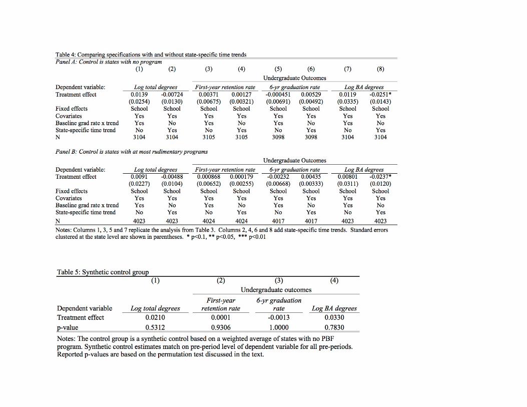
Table 6: Heterogeneity analysis(1) (2) (3) (4) (5) (6) (7) (8) (9) (10) (11) (12)

Undergraduate outcomes

Log total degrees First-year retention rate 6-yr graduation rate Log BA degrees

Panel A: High endowment institutionsTreatment Effect 0.0228 -0.0157 0.0161 0.00603 -0.00972* -0.0043 -0.0161 0.00844 0.0186 0.0218 -0.032 0.0104

(0.0192) (0.0296) [0.4291] (0.00368) (0.00508) [0.8185] (0.0104) (0.00632) [0.4480] (0.0178) (0.0199) [0.4499]

Panel B: Low endowment institutionsTreatment Effect 0.00158 0.0135 0.0456 -0.000875 0.00804 -0.0034 0.0130* -0.00168 -0.0109 -0.00435 -0.0104 0.0254

(0.0323) (0.0228) [0.6900] (0.00887) (0.00672) [0.4783] (0.00645) (0.00873) [0.9959] (0.0437) (0.0193) [0.9017]

Panel C: High graduation rate institutionsTreatment Effect 0.0141 -0.0199 0.0192** 0.00726 -0.00846** -0.004 -0.00204 0.00248 0.0055 0.0218 -0.0229 0.0084

(0.01310) (0.01790) [0.0321] (0.00651) (0.00369) [0.9735] (0.00759) (0.00448) [0.9887] (0.01510) (0.01960) [0.6144]

Panel D: Low graduation rate institutionsTreatment Effect 0.0198 0.00942 0.0522 -0.00205 0.00723 -0.0034 0.00573 0.00947 0.0079 0.00857 -0.0266 0.0485

(0.0579) (0.0165) [0.7483] (0.00856) (0.00450) [0.7222] (0.00836) (0.00813) [0.8733] (0.0598) (0.0190) [0.8785]

Panel E: High state-share of revenue institutionsTreatment Effect -0.00301 -0.0119 0.0291 0.0058 0.00545 0.0063 0.000619 0.0125 0.0092 0.0288 -0.0273 0.0742

(0.0525) (0.0152) [0.8247] (0.0118) (0.00525) [0.7951] (0.00893) (0.0109) [0.8166] (0.0629) (0.0173) [0.5399]

Panel F: Low state-share of revenue institutionsTreatment Effect 0.0354*** -0.00545 0.031 0.0023 -0.000941 -0.0028 0.00249 -0.00443 -0.0069 0.00551 -0.0195 0.0175

(0.0113) (0.0234) [0.2726] (0.00269) (0.00408) [0.9965] (0.00792) (0.00798) [0.6858] (0.0125) (0.0202) [0.6337]

Panel G: Tennessee institutionsTreatment Effect 0.0471*** 0.00566 -0.023 0.0129*** 0.00201 0.003 0.0062 0.00382 -0.0022 0.0586*** -0.0119 0.0244

(0.0138) (0.00754) [0.625] (0.00303) (0.00302) [0.7083] (0.00533) (0.00414) [1.0000] (0.0139) (0.00851) [0.8333]

Panel H: Ohio institutionsTreatment Effect -0.0129 -0.017 0.0663 -0.00355 -0.000248 -0.0018 -0.00557 0.00634 -0.0004 -0.0248 -0.0369** 0.043

(0.0165) (0.0166) [0.4167] (0.00434) (0.00360) [0.9167] (0.00723) (0.00850) [1.0000] (0.0203) (0.0177) [0.5000]Covariates Yes Yes - Yes Yes - Yes Yes - Yes Yes -State-specific time trend No Yes - No Yes - No Yes - No Yes -Synthetic control - - Yes - - Yes - - Yes - - YesNote: The first two columns for each outcome include school and year fixed effects and use states with no PBF as the control group. The control group in the thirdcolumn for each outcome is the synthetic control. Synthetic control estimates show p-values in square brackets. Standard errors clustered at the state level shown inparentheses. * p<0.1, ** p<0.05, *** p<0.01

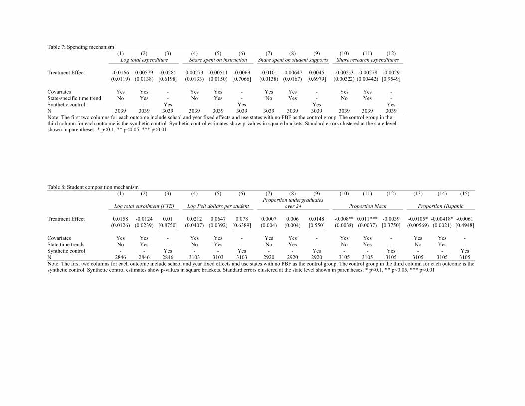
Table 7: Spending mechanism(1) (2) (3) (4) (5) (6) (7) (8) (9) (10) (11) (12)

Log total expenditure Share spent on instruction Share spent on student supports Share research expenditures

Treatment Effect -0.0166 0.00579 -0.0285 0.00273 -0.00511 -0.0069 -0.0101 -0.00647 0.0045 -0.00233 -0.00278 -0.0029(0.0119) (0.0138) [0.6198] (0.0133) (0.0150) [0.7066] (0.0138) (0.0167) [0.6979] (0.00322) (0.00442) [0.9549]

Covariates Yes Yes - Yes Yes - Yes Yes - Yes Yes -State-specific time trend No Yes - No Yes - No Yes - No Yes -Synthetic control - - Yes - - Yes - - Yes - - YesN 3039 3039 3039 3039 3039 3039 3039 3039 3039 3039 3039 3039

Table 8: Student composition mechanism(1) (2) (3) (4) (5) (6) (7) (8) (9) (10) (11) (12) (13) (14) (15)

Log total enrollment (FTE) Log Pell dollars per student Proportion black Proportion Hispanic

Treatment Effect 0.0158 -0.0124 0.01 0.0212 0.0647 0.078 0.0007 0.006 0.0148 -0.008** 0.011*** -0.0039 -0.0105* -0.00418* -0.0061(0.0126) (0.0239) [0.8750] (0.0407) (0.0392) [0.6389] (0.004) (0.004) [0.550] (0.0038) (0.0037) [0.3750] (0.00569) (0.0021) [0.4948]

Covariates Yes Yes - Yes Yes - Yes Yes - Yes Yes - Yes Yes -State time trends No Yes - No Yes - No Yes - No Yes - No Yes -Synthetic control - - Yes - - Yes - - Yes - - Yes - - YesN 2846 2846 2846 3103 3103 3103 2920 2920 2920 3105 3105 3105 3105 3105 3105

Note: The first two columns for each outcome include school and year fixed effects and use states with no PBF as the control group. The control group in thethird column for each outcome is the synthetic control. Synthetic control estimates show p-values in square brackets. Standard errors clustered at the state levelshown in parentheses. * p<0.1, ** p<0.05, *** p<0.01

Proportion undergraduatesover 24

Note: The first two columns for each outcome include school and year fixed effects and use states with no PBF as the control group. The control group in the third column for each outcome is thesynthetic control. Synthetic control estimates show p-values in square brackets. Standard errors clustered at the state level shown in parentheses. * p<0.1, ** p<0.05, *** p<0.01

Figure 1: Event Study Analysis of Effects of PBF 3.0 on Academic Outcomes Panel A: Log Total Degrees Panel B: First-to-Second Year Retention

Panel C: Six-Year Graduation Rate Panel D: Log BA Degrees

Figures show year-over-year results from a regression of the specified outcome on institution and year fixed effects, and a set of indicator variables for years before and after a PBF program was enacted. t-1 is omitted from the regression models so estimated effects are relative to this period. See equation (2) and accompanying explanation in the text for additional details. Standard errors clustered at the state level.

Figure 2: Synthetic Control Analysis of Effects of PBF 3.0 on Academic Outcomes Panel A: Log Total Degrees Panel B: First-to-Second Year Retention

Panel C: Six-Year Graduation Rate Panel D: Log BA Degrees

Figures show results from synthetic control method estimates (Abadie et al 2010). The counterfactual path of the outcome is generated by minimizing all pre-period differences of the dependent variable between treated states and control states. See text for further detail.

Table A1: Control States Used in Analysis

(1) (2)

No-PBF

Control Group At Most Rudimentary PBF Control Group

Alabama Yes Yes Arizona Yes Yes California Yes Yes Colorado Yes Yes Connecticut Yes Yes Georgia Yes Yes Hawaii Yes Yes Idaho Yes Yes Iowa Yes Yes Kansas Yes Yes Kentucky Yes Yes Maryland Yes Yes Massachusetts Yes Yes Michigan - Yes Minnesota - Yes Missouri - Yes Nebraska - Yes New Hampshire Yes Yes New Jersey Yes Yes New Mexico - Yes New York Yes Yes North Carolina - Yes Oklahoma Yes Yes Rhode Island Yes Yes South Carolina Yes Yes South Dakota Yes Yes Texas Yes Yes Utah - Yes Vermont Yes Yes Virginia Yes Yes Washington - Yes West Virginia Yes Yes Wisconsin Yes Yes Wyoming - Yes Source: Author calculations

Table A2: Academic Outcomes Conditional on Student Composition (1) (2) (3) (4) (5) (6) (7) (8)

Undergraduate Outcomes

Log Total Degrees First-year

Retention rate 6-yr Graduation

rate Log BA degrees

Treatment Effect 0.0137 0.0132 0.0037 0.0001 0.0011 0.0017 0.0117 0.0036 (0.0253) (0.0288) (0.0068) (0.0057) (0.0064) (0.0068) (0.0335) (0.0333)

Fixed Effects School School School School School School School School Covariates Yes Yes Yes Yes Yes Yes Yes Yes Baseline Grad Rate x Trend Yes Yes Yes Yes Yes Yes Yes Yes Composition No Yes No Yes No Yes No Yes Observations 3,102 3,103 , 3,102 Notes: The first column for each outcome replicates the analysis from Table 3 but has a few fewer observations due to schools missing student composition data. The second column for each outcome adds the student composition controls to assess whether schools improve outcomes, conditional on composition. Standard errors clustered at the state level reported in parentheses. *p<0.1, ** p<0.05, *** p<0.01

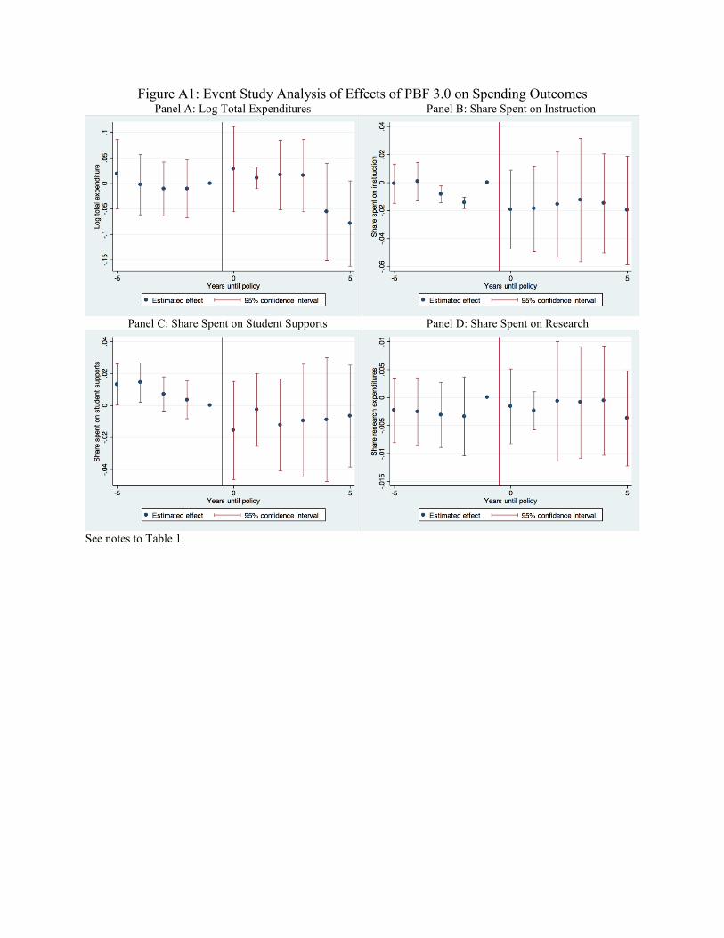
Figure A1: Event Study Analysis of Effects of PBF 3.0 on Spending Outcomes Panel A: Log Total Expenditures Panel B: Share Spent on Instruction

Panel C: Share Spent on Student Supports Panel D: Share Spent on Research

See notes to Table 1.

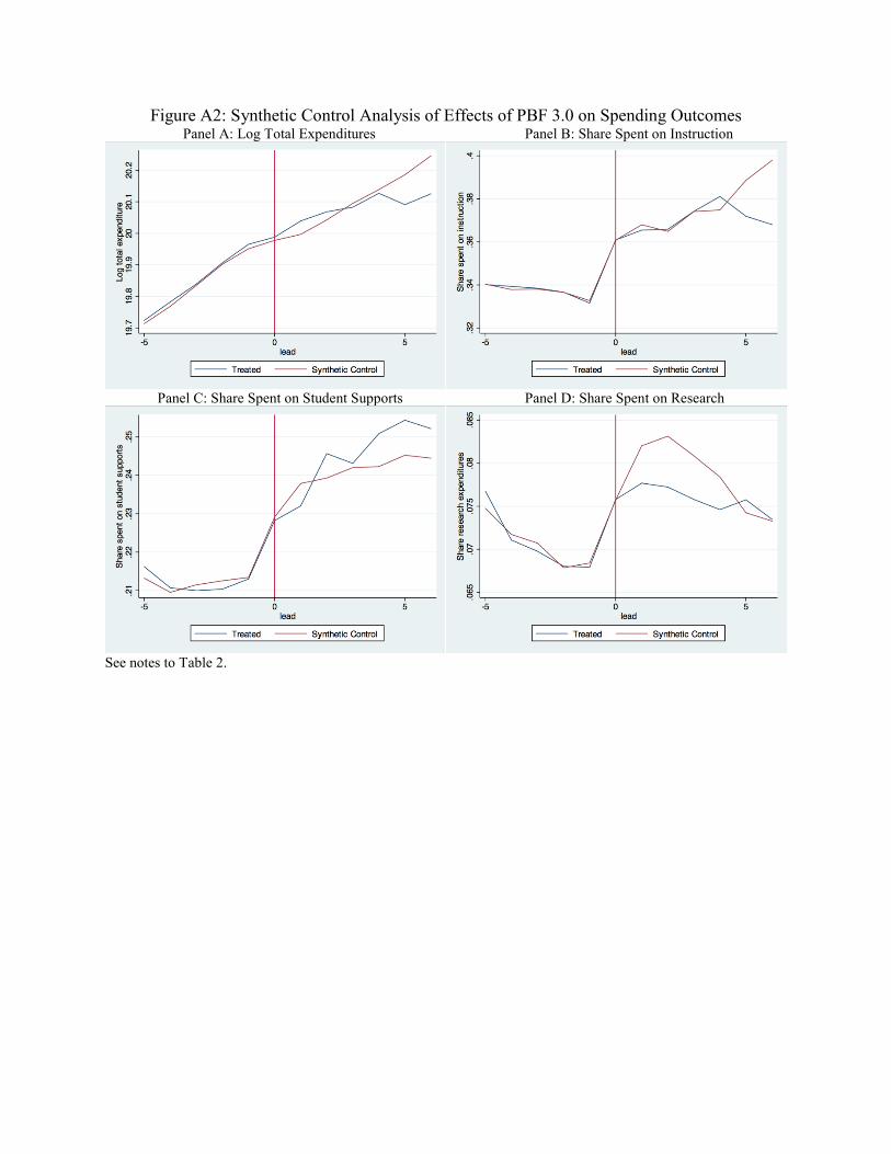
Figure A2: Synthetic Control Analysis of Effects of PBF 3.0 on Spending Outcomes Panel A: Log Total Expenditures Panel B: Share Spent on Instruction

Panel C: Share Spent on Student Supports Panel D: Share Spent on Research

See notes to Table 2.

Figure A3: Event Study Analysis of Effects of PBF 3.0 on Alternate Outcomes Panel A: Log Total Enrollment Panel B: Log Pell Dollars per Student

Panel C: Proportion of Students Over Age 24 Panel D: Proportion of Students Black

Panel E: Proportion of Students Hispanic

See notes to Table 1.

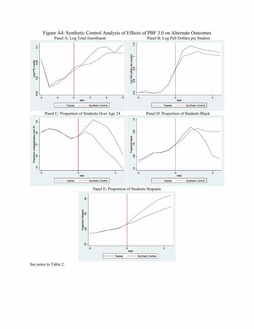
Figure A4: Synthetic Control Analysis of Effects of PBF 3.0 on Alternate Outcomes Panel A: Log Total Enrollment Panel B: Log Pell Dollars per Student

Panel C: Proportion of Students Over Age 24 Panel D: Proportion of Students Black

Panel E: Proportion of Students Hispanic

See notes to Table 2.

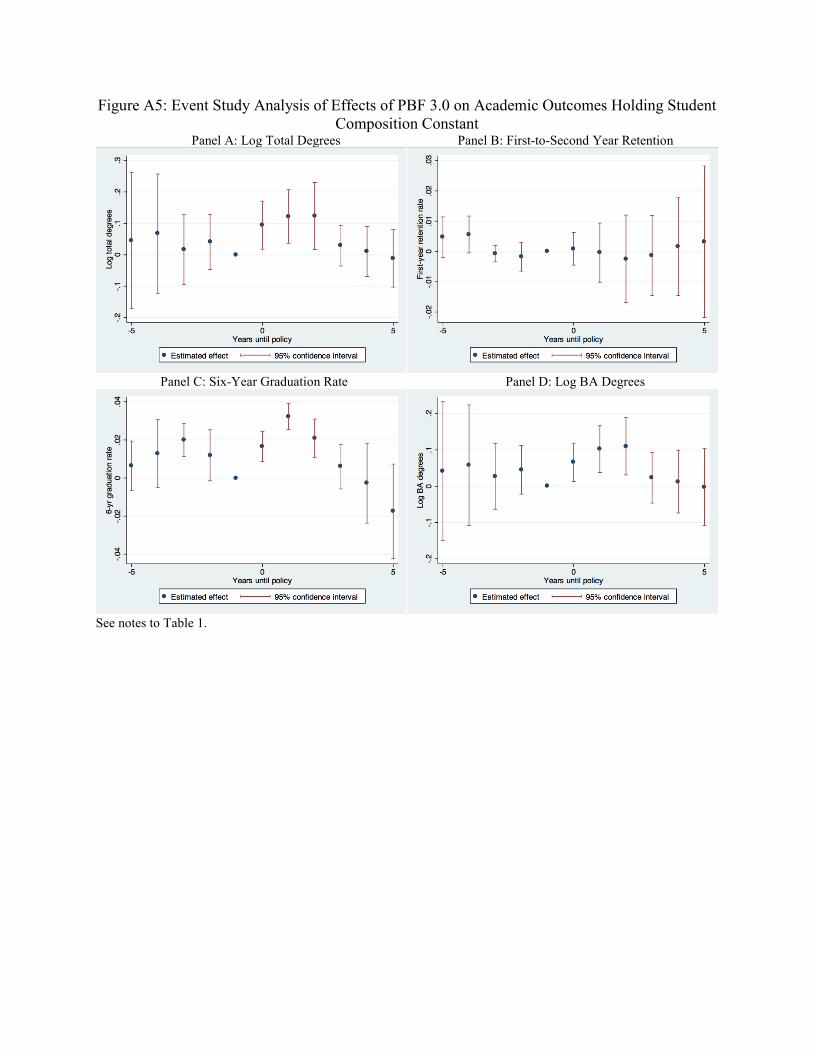
Figure A5: Event Study Analysis of Effects of PBF 3.0 on Academic Outcomes Holding Student Composition Constant

Panel A: Log Total Degrees Panel B: First-to-Second Year Retention

Panel C: Six-Year Graduation Rate Panel D: Log BA Degrees

See notes to Table 1.