the effect of lactobacillus acidophilus ncfm consumption ... · lactobacillus acidophilus ncfm...
TRANSCRIPT
The effect of Lactobacillus acidophilus NCFM
consumption on human intestinal microbial and
metabolite composition
Student Name: Lasse Sommer Mikkelsen
Study Number: 20082043
Supervisors: Artur C. Ouwehand, Henrik M. Jensen and Jette F. Young
Date of submission: 4. March 2014
Collaboration between
And
Preface This master thesis project was made in collaboration with DuPont N&H, Kantvik, Finland and
DuPont N&H, Brabrand, Denmark. The project included investigation of the effect of
Lactobacillus acidophilus NCFM consumption on the level of Clostridium difficile in elderly
subjects, and the effect on microbial metabolic products.
The project was initiated in Kantvik, where fecal samples were collected and weighed out for
the analytical methods used. Furthermore, microbiological analyses (qPCR) and gas
chromatography (GC) analyses were performed in Kantvik. The experimental work in Kantvik
was carried out from March to July, 2013.
A subset of samples was transported to Brabrand, Denmark for nuclear magnetic resonance
(NMR) analysis. Firstly, a preparation and analysis procedure was devised from samples
included in the subset, since fecal samples had not previously been analysed by NMR in
Brabrand. Subsequently, the complete subset was analysed. The experimental work in
Brabrand was performed between August and January 2014.
The methods used and the samples analysed only comprised parts of a larger study concerning
the elderly subjects mentioned above. Furthermore, this master thesis was meant to lay the
ground for further investigations and developments in DuPont N&H, Brabrand.
Abstract During the last two decades, probiotics have become an increasingly popular area of research,
both in terms of its applicability and effect in food products, but especially in terms of its effect
on human health. Additionally, research has also showed a heightened focus on the effect of
the inherent gastrointestinal microbiota on human health. This has resulted in the elucidation
of different mechanisms by which the microbiota and probiotics apply their effects on human
health. The products of the microbial metabolism have also been investigated with the aim of
deducing their roles in relation to human metabolism and health. And several studies have
provided evidence that they have a considerable impact on human metabolism and health.
With ageing, several physiological changes take place, which include changes in the microbial
intestinal composition, but also the inclination of acquiring a wide range of diseases, e.g.
gastrointestinal related diseases. A group of gastrointestinal diseases is termed antibiotic-
associated diarrhea, which covers a special type of diarrhea caused by Clostridium difficile. A
number of studies have demonstrated an effect of probiotics on the prevention of C. difficile-
associated diarrhea. Thus the current study has investigated the effect of probiotic bacterium
Lactobacillus acidophilus NCFM consumption on the level of C. difficile in elderly subjects, and
the effect on microbial metabolic end-products by gas chromatography (GC) and nuclear
magnetic resonance (NMR) analysis. The study did not result in any statistical significant effect
of L. acidophilus NCFM consumption on the level of C. difficile in elderly subjects. In addition,
the consumption of L. acidophilus NCFM was not found to significantly affect the level of acids
analyzed by GC. Based on several preparatory experiments, solubilising fecal samples in
phosphate buffer in a ratio of 1 to 2.5 (fecal weight: buffer volume, mg∙µl-1) was found to be
optimal for nuclear magnetic resonance analysis. From the NMR analyses, 35 compounds were
identified including amino acids, saccharides, organic acids and short-chain fatty acids.
Furthermore, a relatively high correlation between GC and NMR data was also obtained by
relative data comparison, demonstrating the capabilities of NMR as an analytical tool in the
investigation of fecal metabolites.
Resumé Igennem de sidste to årtier er probiotika blevet et mere populært forskningsområde, både med
hensyn til dets anvendelighed og effekt i fødevarer, men specielt med hensyn til dets effekt på
human sundhed. Herudover har forskning også vist øget fokus på effekten af den medfødte
mavetarmflora på human sundhed. Dette har resulteret i udredningen af forskellige
mekanismer, hvormed mavetarmfloraen og probiotika udviser deres effekter på human
sundhed. Produkter fra den mikrobielle omsætning er også blevet undersøgt med henblik på at
udlede deres roller i forhold til human omsætning og sundhed. Her har flere studier vist evidens
for deres betragtelige indflydelse på human omsætning og sundhed. Med aldring finder flere
fysiologiske ændringer sted, hvilket inkluderer ændringer mavetarmfloraens sammensætning,
men også en tilbøjelighed til at pådrage sig en bred vifte af sygdomme, for eksempel mavetarm-
relaterede sygdomme. En gruppe af mavetarm sygdomme er betegnet som antibiotikum-
associeret diarré, hvilket indbefatter en speciel type af diarré forårsaget af Clostridium difficile.
Et antal af studier har demonstreret en effekt af probiotika i forebyggelsen af C. difficile-
associeret diarré. Det indeværende studie har derfor undersøgt effekten af den probiotiske
bakterie Lactobacillus acidophilus NCFM indtag på niveauet af C. difficile i ældre
forsøgspersoner, og effekten på mikrobielle metaboliske slut-produkter ved gaskromatografi
(GC) og kernemagnetisk resonans (NMR) analyse. Studiet resulterede ikke i en statistisk
signifikant effekt af L. acidophilus NCFM indtag på niveauet af C. difficile i ældre
forsøgspersoner. Desuden påvirkede indtaget af L. acidophilus NCFM ikke signifikant niveauet
af syrer analyseret ved GC. Baseret på flere forberedende eksperimenter blev det fundet at
opløse fækale prøver i fosfat-buffer i et 1:2.5 forhold (fækal vægt: buffer volumen, mg∙µl-1) var
optimal for NMR analyse. Af NMR analyserne blev 35 kemiske forbindelser identificeret, hvilke
inkluderede aminosyrer, sakkarider, organiske syrer og kort-kædede fedtsyrer. Yderligere blev
der opnået en relativ høj korrelation mellem GC og NMR ved relativ data sammenligning,
hvilket demonstrerer evnerne for NMR som et analytisk værktøj i undersøgelsen af fækale
metabolitter.

Acknowledgements I would like to thank the scientists and laboratory staff at DuPont N&H in Kantvik, Finland for
their support during my master thesis project. And I would especially like to thank my
supervisors, Sofia D. Forssten and Artur C. Ouwehand, for all their guidance and support during
my stay in Finland, both in and outside the DuPont N&H facilities in Kantvik.
I would also like to thank all the coworkers at the Advanced Analysis department at DuPont
N&H in Brabrand, Denmark for their support during my master thesis. And I would also
especially like to thank my supervisor, Henrik Max Jensen, for his great guidance and support
during my thesis, as well as for his constant enthusiasm and encouragement throughout the
entire project process.
Lastly, I would also like to thank my supervisor, Jette Feveile Young, for her help and guidance
during the entire master thesis project.
List of abbreviations SCFA: Short-chain fatty acids
BCFA: Branched-chain fatty acids
VFA: Volatile fatty acids
qPCR: Quantitative Polymerase Chain Reaction
NMR: Nuclear Magnetic Resonance
CPMG: Carr-Purcell-Meiboom-Gill
NOESY: Nuclear Overhauser Effect Spectroscopy
GC: Gas Chromatography
AAD: Antibiotic-Associated Diarrhea
CDAD: Clostridium difficile-Associated Diarrhea
3OHPPA: 3-(3-hydroxyphenyl)propionic acid
HSQC: Heteronuclear Single Quantum Correlation
TOCSY: Total Correlation Spectroscopy
JRES: J-resolved spectroscopy
ZGESGP: Excitation sculpting pulse sequence
Table of Contents
Preface ............................................................................................................................................................
Abstract ...........................................................................................................................................................
Resumé ...........................................................................................................................................................
Acknowledgements .........................................................................................................................................
List of abbreviations ........................................................................................................................................
1 Introduction ............................................................................................................................................... 1
1.2 Probiotics ............................................................................................................................................ 1
1.3 Microbial life in humans ..................................................................................................................... 2
1.4 Microbial modes of action .................................................................................................................. 3
1.4.1 Microbial competition.................................................................................................................. 4
1.4.2 Intestinal adhesion ....................................................................................................................... 4
1.4.3 Epithelial barrier enhancement ................................................................................................... 5
1.4.4 Anti-microbial compound production and secretion .................................................................. 5
1.4.5 Immunological stimulation and modification .............................................................................. 6
1.5 Microbial metabolism in the human colon ......................................................................................... 8
1.6 Microbes and ageing ......................................................................................................................... 10
1.6.1 Ageing and antibiotic-associated diarrhoea .............................................................................. 11
1.7 qPCR .................................................................................................................................................. 12
1.8 NMR .................................................................................................................................................. 14
1.9 GC ...................................................................................................................................................... 18
2 Materials and methods ............................................................................................................................ 19
2.1 Study design ...................................................................................................................................... 19
2.2 Intervention supplement .................................................................................................................. 19
2.3 Subjects ............................................................................................................................................. 19
2.4 Primary outcome measure ............................................................................................................... 20
2.5 Secondary outcome measures .......................................................................................................... 20
2.6 Additional analyses ........................................................................................................................... 20
2.7 Sample collection and processing ..................................................................................................... 20
2.8 Methods ............................................................................................................................................ 21
2.9 Total Bacterial Count......................................................................................................................... 21
2.9.1 Preparatory phase ...................................................................................................................... 21
2.10 DNA Extraction ................................................................................................................................ 22
2.11 qPCR ................................................................................................................................................ 23
2.12 VFA Analysis .................................................................................................................................... 24
2.13 NMR ................................................................................................................................................ 25
2.13.1 Pre-analysis phase .................................................................................................................... 25
2.13.1.1 Deuterated water extraction: ........................................................................................... 25
2.13.1.2 Deuterated water and methanol extraction (with NaOH and formic acid): ..................... 25
2.13.1.3 Phosphate buffered saline (PBS) buffer extraction .......................................................... 25
2.13.1.4 Testing of NMR pulse sequence ........................................................................................ 26
2.13.1.5 Test of mixing duration ..................................................................................................... 26
2.13.1.6 Sonication and extraction cycles of faecal samples .......................................................... 26
2.13.1.7 Sample weight optimization ............................................................................................. 27
2.13.1.8 Volume-to-sample ratio .................................................................................................... 27
2.13.1.9 Filtration and acid mix spiking of faecal samples ............................................................. 27
2.13.1.10 Biphasic extraction with acid mix spiking of lyophilized faeces ..................................... 28
2.13.1.11 Optimization of NMR pulse sequence ............................................................................ 28
2.13.1.12 Testing of solubilisation method .................................................................................... 29
2.13.1.13 Testing of NH4Cl addition ................................................................................................ 29
2.13.1.14 Testing of pulse sequence, addition of NH4Cl, and dilution of samples ......................... 30
2.13.1.15 Testing of solvent and pulse sequence ........................................................................... 30
2.13.1.16 Additional testing of pulse sequences, sample dilution and preparation procedure .... 30
2.13.1.17 Final testing of pulse sequences, sample dilution and preparation procedure ............. 31
2.13.2 Development of semi-automatic sample preparation system ................................................ 31
2.13.3 Analysis phase .......................................................................................................................... 32
2.13.3.1 Data Acquisition ................................................................................................................ 32
2.13.3.2 Data pre-processing and compound identification .......................................................... 32
2.13.4 Statistical analysis .................................................................................................................... 33
3 Results ...................................................................................................................................................... 35
3.1 qPCR .................................................................................................................................................. 35
3.2 NMR .................................................................................................................................................. 40
3.2.1 Pre-analysis phase ...................................................................................................................... 40
3.2.2 Analysis phase ............................................................................................................................ 42
3.3 GC ...................................................................................................................................................... 60
4 Discussion ................................................................................................................................................. 62
4.1 qPCR .................................................................................................................................................. 62
4.2 NMR .................................................................................................................................................. 63
4.2.1 Pre-Analysis phase ..................................................................................................................... 63
4.2.2 Analysis phase ............................................................................................................................ 65
4.3 GC ...................................................................................................................................................... 67
5 Conclusion ................................................................................................................................................ 67
6 Future perspectives.................................................................................................................................. 68
References .................................................................................................................................................. 68
Appendix A .................................................................................................................................................. 77
(Section 3.1) ............................................................................................................................................ 77
Appendix B .................................................................................................................................................. 86
(Section 3.1, last paragraph) ................................................................................................................... 86
Appendix C .................................................................................................................................................. 90
Pre-analysis phase (section 3.2.1) ........................................................................................................... 90
Appendix D ................................................................................................................................................ 103
Section 3.2.2.......................................................................................................................................... 103
Appendix E ................................................................................................................................................ 128
Appendix F ................................................................................................................................................ 130
Appendix G ................................................................................................................................................ 144
qPCR data used for statistical analysis (section 3.1) ............................................................................. 144
GC data for statistical analysis (section 3.3) ......................................................................................... 154
1
1 Introduction Microorganisms have, in general, been utilized for many years. First in food production and
then later developed for various purposes. One of the best examples, regarding utilization of
microorganisms in food production, is fermented milk. Fermented milk was invented several
millennia ago. At that time, fermented milk was usually made by reusing previously fermented
milk and adding it to fresh milk. This was often done to conserve the milk, which was, and still
is, an important food source. Unaware of the actual cause of the fermentation, people in the
Stone Age did ingest what today would be perceived as ´probiotics´. Even though the concept
and knowledge of probiotics have been under development for many years, it is only during the
last two decades that the scientific community has begun to thoroughly grasp the immense
effects microorganisms have on the entire human body.
The remaining part of the paragraph will provide the basic knowledge on various concepts
related to probiotics, including gastrointestinal microbial composition and function, as well as
describing the technical methods employed in research involving probiotics. Furthermore, the
idea and concept of probiotics will also be described, so to give a general understanding of the
term ´probiotics’.
1.2 Probiotics
Although microorganisms in food production dates back several centuries, even millennia, it
was not until the beginning of the 19th century that the “probiotic concept” was born from a
statement by the Nobel Laureate Ilya Ilyich Metchnikoff in 1907: “…my recommendation to
absorb large quantities of microbes, as a general belief is that microbes are harmful. This belief
is erroneous. There are many useful microbes, amongst which the lactic bacilli have an
honourable place.” (Dobrogosz et al., 2010). Even with the advice from Metchnikoff, the
concept of probiotics did only gradually develop. This, however, changed during the 70s and
80s, mostly due to the rapid evolution and applicability of molecular biological techniques. Also
attention was given to the definition of the “probiotic concept”. Some decades after
Metchnikoff´s suggestion, a definition on the concept had been proposed, and was followed by
another definition a couple of decades after. But it was not until the 80s that a modern
definition of the concept was given by Roy Fuller, where he defined probiotics as: “A live
microbial feed supplement which beneficially affects the host animal by improving its microbial
balance.”(Fuller, 1991). However, this definition was replaced by a new definition adopted at a
joint meeting of experts within Food and Agricultural Organization of the United Nations (FAO)
and World Health Organization (WHO) in 2001, in which it was stated that probiotics are: “Live
microorganisms which when administered in adequate amounts confer a health benefit on the
host.“ (FAO/WHO, 2001). Thus probiotics are live microorganisms, be it archaea, bacteria or
yeast, which will confer one or more health benefit(s) to the host, when ingested in a sufficient
2
amount. Typically, the aspect of survival of the microorganism is self-implied in the definition,
meaning that the microorganism has to survive the passage through the upper gastrointestinal
tract, and have to reach the intended site of effect before inducing a health benefit to the host.
1.3 Microbial life in humans
Although not noticeable, the human body contains a large amount of microbes at various sites,
both in and on the body. And especially in the body, more specifically the gastrointestinal (GI)
tract, the majority of the microbes associated with humans are found. The microbes are
distributed along the entirety of the GI tract from the oral cavity to the colon. Both the oral
cavity and the stomach houses a number of microbes, but the amount is relatively low
compared to the remaining part of the GI tract. Especially the stomach creates an unfavorable
environment with inadequate conditions for the microbes, primarily due to the low pH level,
but also to some degree the relatively rapid transit of ingested food through the stomach. Thus
the number of microbes is considerably low in the stomach with viable bacterial counts in the
range of 102 or less per mL (Macfarlane and Macfarlane, 2012).
When looking at the small intestine, the number of microbes increases. The increase is due to
the more favorable conditions in the small intestine (an increase in pH), which supports
microbial life compared to very low pH levels. However, the upper most and middle part of the
small intestine termed the duodenum and the jejunum is optimized to absorb most of the food
material passing through it, thus leaving little or no food for the microbes to nurture on. Thus in
the duodenal and the jejunal part of the small intestine, the number of bacteria is still relatively
low within the range of 103-105 colony forming units (CFU) per mL. But as the pH level gradually
increases, a concomitant rise in microbial numbers is also observed, reaching a level of up to
109 CFU per mL in the ileum and cecal part of the GI tract (Tiihonen et al., 2010). From the
cecum, a significant rise of microbes is seen; up to a 1000 fold increase immediately adjacent to
the cecum, thus reaching a level of 1012 CFU per mL (Quigley, 2011). An even further increase is
seen along the remaining part of the colon with studies reporting up to a total of 1014 microbial
cells in the colon (Alonso and Guarner, 2013; Arora, 2013).
This vast amount of bacteria is, according to several studies, distributed on a few phyla in the
domain Bacteria, in which the phyla Bacteroidetes, Firmicutes and Actinobacteria contain the
majority of the bacterial genera and species. Microbes from the phyla Proteobacteria and
Verrucomicrobia are also frequently observed, although in lower numbers (Duncan and Flint,
2013). On the other hand, a greater biodiversity is found at both genera and species level with
suggestions of up to 2000 species in the human GI tract (Arora et al., 2013). It should be noted,
however, that the microbiota in one individual are comprised of much fewer species with
reports of up to 160 species in an individual. Furthermore, the GI microbial composition shows
3
high inter-individual differences with a distinctive composition in each individual (Alonso and
Guarner, 2013).
When taking into consideration from which taxonomic category the various microbes originate,
two phyla show dominance, namely Bacteroidetes and Firmicutes. Furthermore, studies have
shown that >90% of the total gut microbiota can be ascribed to these phyla. When diving
further down on the taxonomical scale, a majority of the microbes identified seem to primarily
belong to the genera Bacteroides, Fecalibacterium, and Bifidobacterium. But representatives of
other genera are also found in the microbiota, although making up a lesser part of the
microbiota. Some of these genera are Eubacterium, Clostridium, Ruminococcus, Peptococcus,
Peptostreptococcus, as well as Enterococcus and Lactobacillus.
Another classification concept was suggested a couple of years ago in an extensive study by
Arumugam et al. (2011). In this study, the term `enterotypes´ was introduced. These
enterotypes emerged from principal component analysis (PCA), in which three clusters were
readily discernible. The enterotypes were characterized both according to the abundance of
microbes from a specific bacterial genus, but also according to the variation within this genus.
The assigned genera of the clusters were as follows: Bacteroides (enterotype 1), Prevotella
(enterotype 2), and Ruminococcus (enterotype 3). Furthermore, it was also proposed that
groups of species direct the compositional structure within a given enterotype, indicated by a
strong correlation between the abundant genus in an enterotype and other bacterial genera.
Since enterotypes group people according to their GI microbial composition, it might be
feasible to use this classification system in diagnostics in relation to GI diseases.
1.4 Microbial modes of action
Much research has gone into identifying and measuring the microbes residing in the GI tract,
both with regard to composition and amount of microbes. But just as much effort has been put
into elucidating the various mechanisms by which the microbes function, especially concerning
probiotics. Currently, a number of mechanisms have been established to explain the methods
utilized by the GI microbiota and probiotics (Saad et al., 2013; Gareau et al., 2010; Bermudez-
Brito et al., 2012), contributing to the symbiosis between the human host and the microbiota.
The mechanisms of action can be roughly categorized into either utilizing a physical or
biochemical mode of action with the mechanisms of a physical nature being i) intestinal
adhesion and ii) microbial competition, and the mechanisms of a biochemical nature being i)
epithelial barrier enhancement, ii) anti-microbial compound production and secretion and iii)
immunological stimulation and modification. Although microbial competition would be
classified as a physical mechanism, it is also comprised of elements utilizing a biochemical
mechanism. The following section will elaborate on the individual mechanisms, primarily based
on the information provided in Bermudez-Brito et al. (2012).
4
1.4.1 Microbial competition
Colonic microbial competition is comprised of a couple of mechanisms. One of these is the
competition for nutrients. The idea behind this mechanism is that the probiotics will
outperform the pathogens in the colon regarding food sources, thus aid in avoiding pathogen-
induced diseases. Another option for the probiotics is to create a hostile microenvironment
toward pathogens. This mostly includes lowering the pH in the immediate area around the
probiotic cells, which is unfavorable for many pathogenic bacteria. Additionally, the probiotics
also produce a range of antimicrobial compounds as well as metabolites, which are secreted
from the cells and actively contribute to the creation of a hostile environment. Furthermore,
probiotics can also occupy several bacterial receptor sites, thus denying pathogens the
possibility of adhere to the intestinal epithelium. All of the above options support the probiotic
strategy of excluding, and to some degree, eliminating pathogens within the intestines. This
exclusion method was for instance shown in a study by Coconnier et al. (1993), in which a
Lactobacillus strain was able to physically exclude pathogens from the intestinal surface. In a
review by Schiffrin and Blum (2002), they make a distinction between bacterial
intercommunication and host-bacteria interaction. And here they also mention several
components, such as antimicrobial compounds and metabolite, modification of redox potential
and O2 consumption etc., which all support the over-all pathogenic exclusion strategy. This
emphasizes the importance of these elements as a barricade against external pathogenic
attacks. Since some of the elements mentioned in microbial competition are based on the other
proposed mechanisms of action, some are described in more detail below.
1.4.2 Intestinal adhesion
Some intestinal microbes are primarily found in the luminal content, whereas others are
located at the epithelial surface, either adhering to intestinal epithelial cells (IECs) or to the
mucous layer covering the IECs. And this adhesion to the intestinal surface is considered to be
another mechanism of action of probiotics. By adhering to the intestinal surface, probiotics
both exclude pathogens as described below, but are also able to form colonies in the intestines.
The primary component of mucous is mucins, large glycoproteins secreted into the intestine to
protect the intestinal surface. In order to adhere to either the IECs or mucous layer, probiotics
use surface proteins to interact, and attach themselves to the mucous layer or the intestinal
surface. Besides the physical hindrance provided by the adhesion, communication with the host
in terms of immune responses, both innate and adaptive, is also facilitated. And in this regard,
probiotics have shown to affect host cells´ release of defensive molecules, such as lysozyme or
phospholipase A2 and defensins acting on the bacterial cell wall or bacterial membrane,
respectively, and thereby disrupting and destroying the cell (Müller et al., 2005; Koprivnjak et
al., 2002).
5
1.4.3 Epithelial barrier enhancement
Between the epithelial cells comprising the top layer of cells in both the small and large
intestine, a small gap is found referred to as tight junctions. The gaps in the tight junctions are
spanned by proteins, which connect adjacent epithelial cells. If these tight junctions are not
kept well tightened, a range of molecules from the intestinal lumen can pass through these
junctions and cause a variety of adverse effects. In some cases, cells can pass through these
junctions and cause diseases. Another of the putative mechanisms for probiotics is to improve
these tight junctions, thus enhancing the epithelial barrier against entrance of unwanted
molecules. Some studies report that this mechanism has been utilized by some lactobacilli
strains as well as the probiotic mixture named VSL#3, which contains eight different bacterial
strains: Lactobacillus acidophilus, L. delbrueckii subsp. bulgaricus, L. casei, L. plantarum,
Bifidobacterium longum, B. infantis, B. breve and S. thermophilus (Saad et al., 2013). The studies
found that the lactobacilli and VSL#3 were able to either modulate or increase the expression of
proteins associated with tight junctions (Hummel et al., 2012; Dai et al., 2012). Another possible
mechanism linked to barrier enhancement is the regulation of mucin production and secretion
by probiotics, contributing to the epithelial barrier. Although fewer studies have been
conducted on this particular subject, some reports have been made providing evidence for
probiotics affecting mucin production (Bermudez-Brito et al., 2012).
1.4.4 Anti-microbial compound production and secretion
Another mechanism utilized by probiotics is to provide the intestinal environment with anti-
microbial compounds, termed bacteriocins. These bacteriocins are often proteins, which either
inhibit the cell proliferation of pathogens or cause cell destruction. But other molecules can
also induce inhibitory effects on pathogens including several metabolites. Especially organic
acids, such as lactic acid, and SCFAs, e.g. acetic acid have both shown to be very potent as anti-
microbial compounds (Alakomi et al., 2000; De Keersmaecker et al., 2006; Makras et al., 2006).
These substances induce their effects on chemical or biochemical features of a pathogenic cell,
such as disrupting the cell membrane, or making changes to the pH equilibrium in the cell. A
further elaboration on the various effects of SCFAs and other metabolites on the host will be
given in a later section.
6
1.4.5 Immunological stimulation and modification
A wealth of research has gone into investigating this particular mechanism. And as noted by Gill
and Prasad (2008) the studies date back several decades, where it became generally accepted
that the endogenous microbiota have a significant effect on the activity and development of
our immune system. The importance of the microbiota has been shown in several studies by
using germ-free mice, and as pointed out by Alonso and Guarner (2013) not only the immune
function was affected in germ-free mice, the lack of microbes also induced an increase in food
ingestion and a reduction in the development of certain organs.
As stated above, the commensal bacteria in the intestines and probiotics can both modify and
stimulate the immediate immune responses (the innate immune system) and the long-term
immune response (the adaptive immune system).
The innate immune system functions by recognizing several molecular patterns found on
pathogens, involving pattern recognition receptors (PRRs) on host cells. The interaction
between PRRs and the pathogen patterns leads to a cascade of biochemical reactions and cell
intercommunication, ultimately resulting in elimination of pathogens. The PRRs include the
Toll-like receptor (TLR) family, which have been studied extensively. But other PRRs also exist,
such as nucleotide-binding oligomerization domain-containing protein (NOD)-like receptors,
termed NLR. Probiotics have shown in several studies that they are capable of modulating the
PRRs both in terms of the expression and effect of PRRs. Regarding the expression of PRRs,
probiotics seem to have a stimulatory as well as an inhibitory effect. The former was shown in a
study, where a Lactobacillus strain had been administrated to healthy mice. After
administration, the expression of TLR2, TLR4 and TLR9 had been increased (Castillo et al., 2011).
In contrast, a study by Liu et al. (2012) showed that administration of L. reuteri strains to rats
with necrotizing enterocolitis (NEC) induced down-regulation of TLR4 and molecules involved in
immune responses. Furthermore, the probiotic L. rhamnosus GG has shown to lower the
production of interleukin-8 (IL-8) and tumor necrosis factor α (TNF-α), two major cell
attractants in the immune responsive pathway in IECs and activated macrophages, respectively
(Zhang et al., 2005; Pena and Versalovic, 2003). The effect on IL-8 and TNF-α production is most
likely due to a modulation of one or more PRRs. Thus probiotics have the ability to either
stimulate or reduce immune responses, depending on factors such as probiotic strain, host
situation (infectious state vs. non-infectious state) etc. Most often, however, it is a reduction or
anti-inflammatory effect that is sought from probiotics, especially during an infection or an
inflammatory state, such as in inflammatory bowel disease.
Not only have probiotic studies provided the evidence for an effect on the innate immune
system, several studies have also found an effect of probiotics on the adaptive immune system.

7
In contrast to the innate immune system, the adaptive immune system does not show
immediate reactions to pathogenic attacks, but is effective over a longer period.
The adaptive immune system shares similarities with the innate immune system. However, the
adaptive immune system is primarily initiated by antigen presentation. Specific immune cells
(B-cells) can digest pathogens and present molecules originating from these pathogens to other
immune cells (T-cells). The presentation of antigens causes a range of biochemical reactions
and microbiological interactions, causing the production of specific antibodies
(immunoglobulins, Ig). The B-cells produce antibodies on stimulation by T-cells, which are also
capable of eliminating infected cells (cytotoxic T-cells, Tc).
Regarding the Ig production and secretion, several studies indicate an effect of probiotics on
this aspect of the adaptive immune system. This was for example shown in a study with
colorectal cancer patients, who had gone through surgery. Here, the administration of
probiotics during a 7 days period resulted in an increase of several Igs (Zhu et al., 2012). Similar
results was obtained in a study by Kaila et al. (1992), where a Lactobacillus strain had been
given to small children (mean age 16 months) during a rotavirus infection. Relatively large
increases in IgG, IgA and IgM were observed for the children receiving the probiotic strain. And
in continuation, a Japanese study also found an increase in IgA during consumption of the
probiotic strain B. lactis Bb-12, subsequent to a polio vaccination in children (age range: 15-31
months) (Fukushima et al., 1998). But not only have effects of probiotics on Ig production and
secretion been observed, several studies also report on the effect of probiotics on the number
and activity of immune cells, such as Gill et al. (2001), where elderly subjects consumed a milk
product containing B. lactis HN019. This resulted in a marked increase in both the activity of
phagocytes and natural killer (NK) cells, which have a similar function and activity as TC cells.
Furthermore, it was also seen that the amount of NK cells and T cells rose during the
consumption of the probiotic bacteria. In addition, Nagao et al. (2000) found that when study
subjects consumed a fermented milk product containing L. casei Shirota, the level and activity
of NK cells increased. On the contrary, no probiotic effect was observed for T cells.
8
1.5 Microbial metabolism in the human colon
As mentioned earlier, the human colonic microbiota produces a number of metabolites, among
which SCFAs constitute the majority. The SCFAs are primarily derived from saccharolytic
microbial fermentation of non-digestible polysaccharides, as well as polysaccharides escaping
the digestion in the upper GI tract, e.g. resistant starch. The SCFAs are, however, not produced
to the same degree, and is typically found in a 60:20:20 molar ratio (acetate : propionate :
butyrate) with an estimated decrease of 70-140 mM to 20-70 mM from the first part of the
colon to the last part of the colon, respectively (Wong et al., 2006). Therefore, concentrations
found in fecal samples can only partially reflect the actual concentrations within the colon,
mainly confined to the lower part of the colon. Based on the fact that substrates for colonic
fermentation come from ingested food, diet has a pivotal influence on the composition and
concentration of, not only SCFAs produced, but also on the composition of the intestinal
microbiota in general. As described above, a myriad of bacteria harbour the GI tract, providing a
variety of different functions related to fermentation, which is very well illustrated in
Macfarlane and Macfarlane (2012). This also induces a level of co-dependence between
bacterial groups, along with the concept of cross-feeding. Here, fermentation products of
certain bacteria are utilized by other bacteria for energy generation. This was for instance
found in a study by Marquet et al. (2009), where lactate from fermentation was used by butyric
acid-producing bacteria, as well as a sulphate-reducing species. In general, the level of lactate is
relatively low within the colon (Macfarlane and Macfarlane et al., 2012) despite several
members of the colonic microbiota produce lactate during fermentation.
SCFAs not only give rise to changes within the colon by reducing pH levels, but have also been
found to affect the physiology of the host. The most abundant SCFA, acetic acid, have been
found to be one of the main substrates for cholesterol synthesis within humans (Wong et al.,
2006). However, the effect on lipid metabolism is not well established for this SCFA.
Propionate has also been suggest to be involved in host metabolism based on a number of
studies, both as a regulator of cholesterol metabolism and of carbohydrate metabolism
(glycolysis and gluconeogenesis) (Wong et al., 2006). However, the exact role in host
metabolism has not been elucidated, due to inconsistency among studies. Furthermore, other
studies have provided evidence that propionate may also play a role in certain immunological
and neurological aspects (Macfarlane and Macfarlane, 2012 (Table 3)).
The last SCFA, butyrate, is proposed to be the primary source of energy production in
colonocytes, acting as a substrate for 60-70 % of the energy generated (den Besten et al.,
2013). In addition to its metabolic function in colonocytes, butyrate has also been found to
regulate several cellular functions, e.g. acetylation of histone proteins in chromatin (Sealy and
Chalkley, 1978). Furthermore, butyrate is also suggested to be involved in colon cancer
prevention (Bornet et al., 2002). Moreover, several studies have also indicated that butyrate
plays a role in various immunological aspects (Macfarlane and Macfarlane, 2012).
9
However, not only carbohydrates are used for fermentation. A range of nitrogen-containing
compounds are also converted by colonic microbial fermentation to a number of end products.
This includes the degradation of amino acids to branched-chain fatty acids (BCFAs), comprised
of isobutyrate, 2-methylbutyrate and isovalerate, which are formed from the branched-chained
aliphatic amino acids valine, isoleucine and leucine, respectively (Smith and Macfarlane, 1997).
Consequently, by-products of the amino acid degradation are also released in the colon (e.g.
ammonia, CO2), but also nitrogenous compounds such as putrescine, agmatine and cadaverine.
Furthermore, products from aromatic amino acid degradation are also found in the colon (e.g.
indole and phenol).
The group of compounds described so far only covers major components of the diet, namely
polysaccharides and proteins. However, due to the variety of foods consumed in the human
diet, other chemical food components are also ingested, although in minor amounts compared
to proteins and polysaccharides. One such group of food components are polyphenols, which
are ubiquitously found in a wide range of fruits and vegetables. These components contain
hydroxylated phenyl moieties, and are classified into several distinctive groups depending on
their specific chemical structure (Cardona et al., 2013). Many of these polyphenolic compounds
have been investigated in vitro and in vivo, but also in human intervention studies (Bolca et al.,
2013). Furthermore, several of these studies have found an effect of polyphenols on the
organism studied, be it microbes, animals or humans. One such study was carried out by
Tzounis et al. (2011), where consumption of cocoa-derived polyphenols (flavanols) by healthy
humans induced changes to the microbiota and inflammatory markers. In general, studies
indicate that polyphenols affect the immune system, and also play a role in cancer prevention
(Cardona et al., 2013).
Another polyphenolic class is based on hydroxycinnamic acids, which comprise up to half of the
polyphenols consumed in food, according to Clifford (2004). A compound from this particular
polyphenolic class (caffeic acid) has been shown to be degraded by colonic microbes into 3-(3-
hydroxyphenyl)propionic acid (3OHPPA) in a study by Konishi and Kobayashi (2004).
Furthermore, a recent in vitro study, based on a human faecal sample, reported that 3OHPPA is
the primary metabolite of caffeic acid (Parkar et al., 2013). In the same study, 3OHPPA was also
found to increase the proliferation of Bifidobacterium longum and the concentration of SCFAs
based on a faecal slurry sample, indicating that polyphenolic compounds not only affect
humans, but also the endogenous microbiota. Due to the high inter-individual differences in the
GI microbial composition, the ability of the microbiota to metabolize polyphenolic compounds
also display marked differences, leading to inter-individual variances regarding the degradation
and conversion of polyphenolic compounds, as pointed out in Bolca et al. (2013).
10
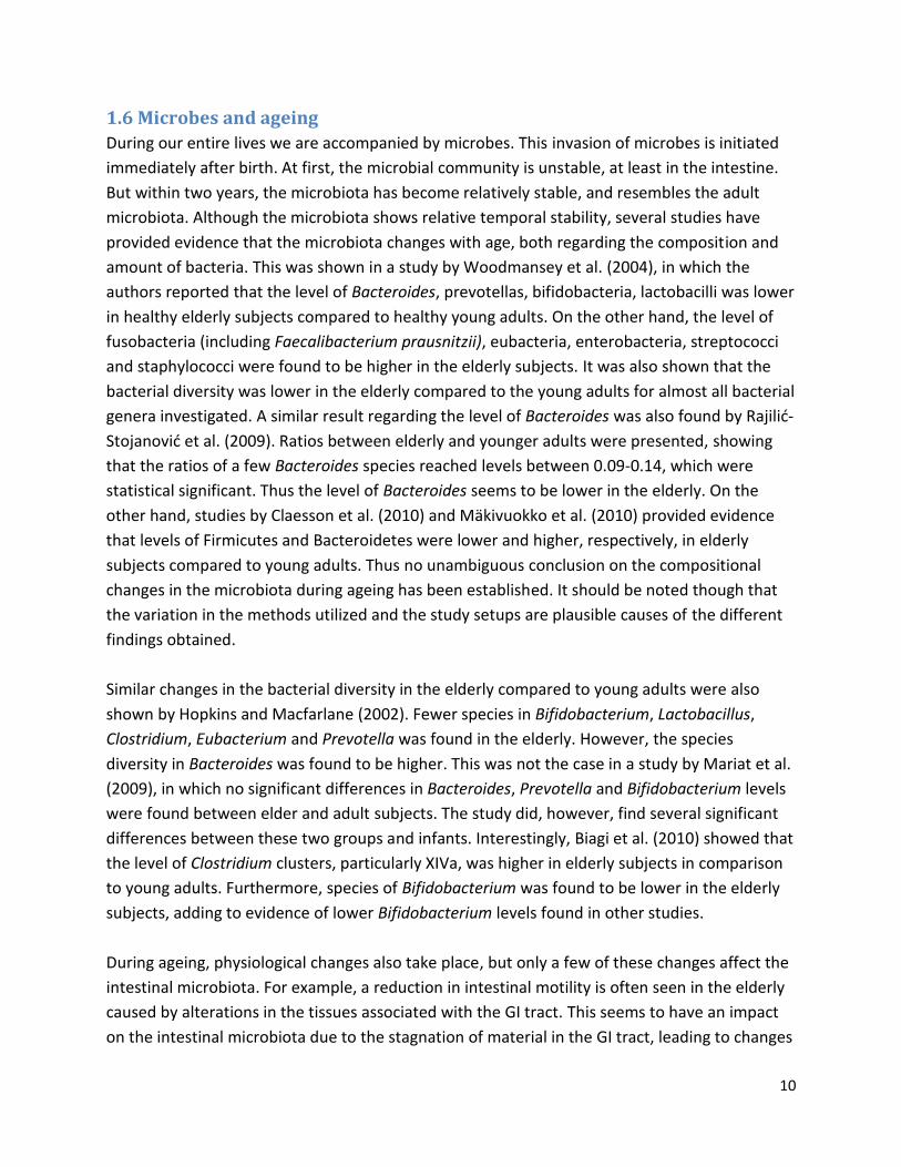
1.6 Microbes and ageing
During our entire lives we are accompanied by microbes. This invasion of microbes is initiated
immediately after birth. At first, the microbial community is unstable, at least in the intestine.
But within two years, the microbiota has become relatively stable, and resembles the adult
microbiota. Although the microbiota shows relative temporal stability, several studies have
provided evidence that the microbiota changes with age, both regarding the composition and
amount of bacteria. This was shown in a study by Woodmansey et al. (2004), in which the
authors reported that the level of Bacteroides, prevotellas, bifidobacteria, lactobacilli was lower
in healthy elderly subjects compared to healthy young adults. On the other hand, the level of
fusobacteria (including Faecalibacterium prausnitzii), eubacteria, enterobacteria, streptococci
and staphylococci were found to be higher in the elderly subjects. It was also shown that the
bacterial diversity was lower in the elderly compared to the young adults for almost all bacterial
genera investigated. A similar result regarding the level of Bacteroides was also found by Rajilić-
Stojanović et al. (2009). Ratios between elderly and younger adults were presented, showing
that the ratios of a few Bacteroides species reached levels between 0.09-0.14, which were
statistical significant. Thus the level of Bacteroides seems to be lower in the elderly. On the
other hand, studies by Claesson et al. (2010) and Mäkivuokko et al. (2010) provided evidence
that levels of Firmicutes and Bacteroidetes were lower and higher, respectively, in elderly
subjects compared to young adults. Thus no unambiguous conclusion on the compositional
changes in the microbiota during ageing has been established. It should be noted though that
the variation in the methods utilized and the study setups are plausible causes of the different
findings obtained.
Similar changes in the bacterial diversity in the elderly compared to young adults were also
shown by Hopkins and Macfarlane (2002). Fewer species in Bifidobacterium, Lactobacillus,
Clostridium, Eubacterium and Prevotella was found in the elderly. However, the species
diversity in Bacteroides was found to be higher. This was not the case in a study by Mariat et al.
(2009), in which no significant differences in Bacteroides, Prevotella and Bifidobacterium levels
were found between elder and adult subjects. The study did, however, find several significant
differences between these two groups and infants. Interestingly, Biagi et al. (2010) showed that
the level of Clostridium clusters, particularly XIVa, was higher in elderly subjects in comparison
to young adults. Furthermore, species of Bifidobacterium was found to be lower in the elderly
subjects, adding to evidence of lower Bifidobacterium levels found in other studies.
During ageing, physiological changes also take place, but only a few of these changes affect the
intestinal microbiota. For example, a reduction in intestinal motility is often seen in the elderly
caused by alterations in the tissues associated with the GI tract. This seems to have an impact
on the intestinal microbiota due to the stagnation of material in the GI tract, leading to changes
11
in the local environment. Furthermore, saliva secretion is also seen to be lowered in the elderly,
which affect the mucosal health (Tiihonen et al., 2010).
The ageing process also induces a deterioration of the immune system, and compared to other
age-related physiological changes, this seem to have a considerable effect on the intestinal
microbiota. The overall concept has been termed immunosenescence, and influences both the
innate and the adaptive immune system. In normal, well-functioning intestines, the microbial
community is constantly surveyed by the epithelial cells, and in close cooperation with the
immune cells, keeping the interaction between the microbiota and the host under control and
immune cells in close cooperation. This status changes during ageing, in which a chronic, low
grade inflammatory situation occurs, coined `inflamm-ageing´ (Biagi et al., 2013).
As mentioned above, probiotics seem to exert an effect on development and function of the
immune system. And not only in infants and adults, but also in the elderly, which is particularly
needed taking immunosenescence into consideration. This was shown in a study by Ibrahim et
al. (2010), where elderly subjects consumed a probiotic cheese, resulting in increased activity
and amount of granulocytes and monocytes. Furthermore, the cytotoxicity of peripheral blood
mononuclear cells (PBMCs) was also increase during consumption.
Due to `inflamm-ageing´, the microbial composition also changes causing the protective effect
of the microbiota to be less effective, and potentially increasing the risk of infections and
diseases, such as a Clostridium difficile infection.
1.6.1 Ageing and antibiotic-associated diarrhoea
Although the GI microbiota is typically very stable, it can be destabilised. This is for instance the
case during antibiotic treatment. Antibiotics, especially broad-spectrum antibiotics, can cause
elimination of several members of the microbiota, disturbing the compositional balance and
function of the microbiota, leading to the phenomenon known as antibiotic-associated
diarrhoea (AAD), which has been reported to occur in 5-25 % of patients on an antibiotic
treatment (Bartlett, 2002). Furthermore, a special type of AAD is caused by the opportunistic
pathogen, Clostridium difficile, thus termed C. difficile-associated diarrhoea (CDAD), which
account for 15-25 % of AAD case, as stated by Katz (2006). Due to the disturbances of the
microbiota inflicted by antibiotics, the members of the microbiota can no longer exert their
normal modes of action (see section 1.4, and Britton & Young, 2012 (Fig. 1)), leading to an
overgrowth of C. difficile. Furthermore, C. difficile also produces two types of exotoxins, A and
B, which are the primary cause of symptoms observed during C. difficile infection (Lessa et al.,
2012). Although uncomfortable, diarrhoea is a mild symptom in C. difficile infection, which can
develop into more severe disease states including pseudomembranous colitis and toxic
megacolon (Keller and Surawicz, 2014). Furthermore, one of the most important risk factors for
C. difficile infection, in addition to antibiotic treatment, is age as noted by Keller and Surawicz
(2014) (Table. 1), especially elderly from 65 years of age. Most often, C. Difficile is acquired in
12
health-care settings, due to a prevalence of C. difficile spores (Weber et al., 2013). However,
some studies have reported that a large percentage of C. difficile infections, up to 50 % (Keller
and Surawicz, 2014), were acquired in a long-term care facility, such as a nursing home or
elderly home, indicating that the pathogen can also frequently be found in such facilities.
The exact mechanism of the microbiota to prevent C. difficile from causing diseases is not
known, but it is likely a combination of the mechanisms of action suggested above. Based on
the effect of the microbiota, much interest has been given to probiotics, since they exert their
effect in the GI tract in a similar manner. Several studies have been performed, investigating
the effect of probiotics on both ADD and CDAD. Regarding the effect of probiotics on AAD,
studies have achieved contradictory results (Katz, 2006 (Table1)). However, in a study by Gao et
al. (2010), probiotics were given to hospitalized patients in addition to their antibiotic
treatment. Here it was found that patients consuming L. acidophilus CL1285 and L. casei
LBC80R had a lower incidence of AAD and CDAD than in the placebo group. Furthermore,
another similar study investigated the effect of probiotics on AAD and CDAD incidences. The
probiotics used in this study included L. casei DN-114 001, Streptococcus thermophilus, and L.
bulgaricus. This study also resulted in a reduction in the incidence of AAD and CDAD in the
probiotic group compared to the control group (Hickson et al., 2007). Moreover, in a meta-
analysis by McFarland et al. (2006) it was concluded that probiotics had a significant effect on
the reduction of C. difficile disease. However, the randomised controlled trials did differ on
several important study aspects (probiotic strain and dose usage, duration of treatment etc.),
resulting in different outcomes. Therefore, the effect of probiotics on the development of
infection by C. difficile in connection with antibiotic treatment is not completely clear.
1.7 qPCR
There are several techniques to exploit, when a specific DNA fragment is to be cloned. But even
though several methods exist, it was not until the 1980s that the powerful polymerase chain
reaction (PCR) was invented. The technique makes it possible to rapidly amplify a DNA
fragment or segment of interest, ending up with millions of copies of that specific fragment or
segment.
PCR can be described as follows: Firstly, DNA is isolated before starting the PCR. After DNA
isolation, DNA is heated in order to separate the double-stranded DNA (dsDNA) containing the
DNA fragment of interest. After heating, primers are added to the DNA, which is then allowed
to anneal to the single-stranded DNA. Subsequently, DNA polymerase is added to the mixture
which elongates the primer resulting in a new pair of dsDNA, thus ending cycle 1. This means
that a doubling of dsDNA pairs have occurred after one cycle. After another cycle, the number
of dsDNA pairs has doubled again. Thus each cycle results in a doubling of the DNA pairs, which
accumulate to the already existing DNA. Since the number of DNA pairs is doubled each cycle,
13
the total number of DNA pairs can then be calculated by the following formula: Total number of
DNA pairs = 2n, where n is the number of cycles. The process is then repeated, typically
between 20-40 cycles, thus resulting in 220-240 dsDNA pairs.
The quantitative PCR method (also known as real-time PCR) is based on the original PCR
method. But in addition to creating a large amount of DNA copies of a targeted DNA fragment,
the qPCR method also makes it possible to quantify the amount of DNA. This is done by adding
either a fluorescent probe or a dye to act as reporters. The dye binds to dsDNA by intercalating
between the two strands. Furthermore, the intercalated dsDNA is excited by light of a specific
wavelength. After absorption of the light, an amount of light is emitted from the intercalated
dsDNA at a specific wavelength resulting in a signal. Since the dye binds to dsDNA, an
exponential increase will occur after each cycle. One of the most common dye techniques is
referred to as SYBR green, which was also used in the present study.
When using a probe containing a fluorophore, another mechanism is exploited. The probe is
designed specifically for the gene of interest. The probe is a small DNA fragment
(oligonucleotide) on to which a fluorescent reporter and a quencher have been attached. The
scheme for the probe PCR assay is as follows: An amount of probe containing the fluorophore is
added to the DNA. After the first step separating the dsDNA by heating, not only the primers
will anneal to the DNA templates, but also the probe. After annealing, the polymerase binds to
the DNA templates and starts the elongation phase. When it encounters a probe attached to
the DNA template, it will degrade the probe. By this degradation, the fluorescent reporter is
cleaved and released from the probe, on which the quencher is still attached. After each cycle,
an energy source excites the sample, leading to absorption and emission of light from the
released fluorophore, thus resulting in a detectable signal.
As mentioned above, the dye binds to all dsDNA, which also implies binding to e.g. primer
dimers (dsDNA complex made up of the forward and reverse primers). This can then lead to
erroneous results in which those signals would be included as well. This is avoided, when using
a fluorescent probe assay, since the probe only binds to a very specific part of the DNA
template. Thus no signal or increase in signal is detected, if the probe has not annealed to a
DNA template and been degraded (VanGuilder et al., 2008).
14
1.8 NMR
Both qPCR and GC are based on primary physicochemical features of molecules, such as the
polarity of a specific molecule (in GC), or the energy level at which separation of double-
stranded DNA occur, as well as the energy level at which primers and probes can anneal to
complementary DNA segment via hydrogen bonds (in qPCR). In comparison, NMR is not only
based on chemical properties of molecules, such as solubility or acidity/alkalinity, but it is also
based on the physical nature of the atoms. A vast amount of parameters affect the NMR
method and the manner in which it analyses a particular sample, thus only a brief description of
the NMR method and the concept on which it is build will be given here.
NMR is based on the fact that nuclei with odd numbered atomic mass, such as 1H and 13C
possess a nuclear spin. The different nuclei have different spins, but the spins are only found in
specific states given by the spin quantum number, S. These spins can only occur in discrete
integer or half-integer values, in which the most common are spins with S = ½. When such
spinning nuclei are placed in an external magnetic field (B0), they will align along the axis of the
external field. Furthermore, nuclei with S = ½ can only occur in one of two states, either parallel
with or anti-parallel to the direction of B0. Subsequently to placing the nuclei in an external
magnetic field, the spins will start to rotate or precess around the axis of the external field at a
specific frequency. This precession around the axis of B0 is, however, not measurable in NMR.
In order to make the precession measurable, an energy input equal to the rate of precession or
frequency is required (also known as the Larmor frequency). In modern NMR devices, this is
overcome by transmitting a radio frequency (RF) pulse to the sample under investigation. This
energy is then absorbed by the nuclei precessing at the specified frequency, forcing the nuclei
away from the axis of B0. By convention, a three-dimensional Cartesian coordinate system is
applied to a magnetic field in NMR, in which the direction of B0 is placed along the z-axis. After
forcing the nuclei away from the axis of B0, the nuclei will now start to precess around another
axis in the coordinate system. The new axis around which the nuclei will start to precess is
usually the +y axis, depending on the direction of the pulsed RF. The nuclei precess around the
new axis until the pulse is turned off. Since the nuclei are no longer forced away from the z-axis,
they stop precessing around the current axis and start to precess around the z-axis, but now the
precession occur in the x-y plane of the coordinate system. Eventually, the precessing nuclei
will return to their original state in the external field with a simultaneous emission of energy.
This energy is absorbed by RF coils in close proximity to the sample being examined, and after
computational tasks this energy absorption will lead to the production of a spectrum.
Another characteristic of nuclei possessing spin is their ability to couple to each other, referred
to as spin-spin coupling (sometimes also referred to as `sensing´ to improve the perception of
15
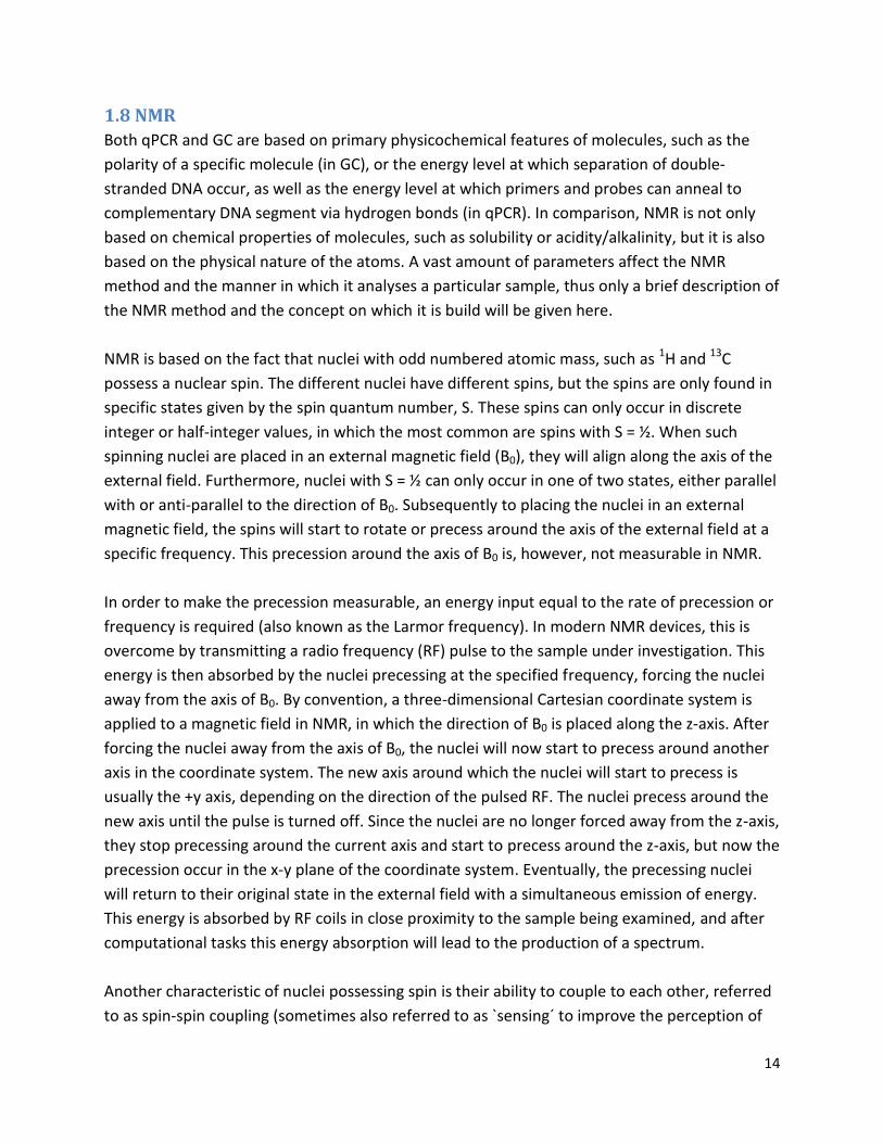
the coupling concept). Both heteronuclear (C-H) and homonuclear (H-H) coupling can be
observed, but here the primary focus will be on H-H coupling. This is exemplified with propionic
acid in Fig. 1.
Figure 1 Multiplet determination and coupling of propionic acid Each chemical groups exhibiting coupling (-CH2-, CH3) have been assigned to the appropriate signal.
The two hydrogen nuclei in the -CH2- group in propionic acid are thought of as identical; they
`feel´ the same magnetic environment, and have the same chemical shift (precession rate in
Hz). Even though the two hydrogen nuclei couple to each other, this coupling is not displayed in
a spectrum, because they have the same chemical shift. The two hydrogen nuclei does,
however, couple to the 3 hydrogen nuclei in the CH3- group, which is shown as four lines
connected to each other (termed a quartet). The reason for this specific pattern is that both
hydrogen atoms in the -CH2- group are equally coupled to the 3 hydrogen atoms in the CH3-
group. Each of the hydrogen nuclei in the CH3- group will split the -CH2- signal into two, thus
giving the pattern depicted in Fig. 2
Propionic acid
-CH2- group
CH3- group
16
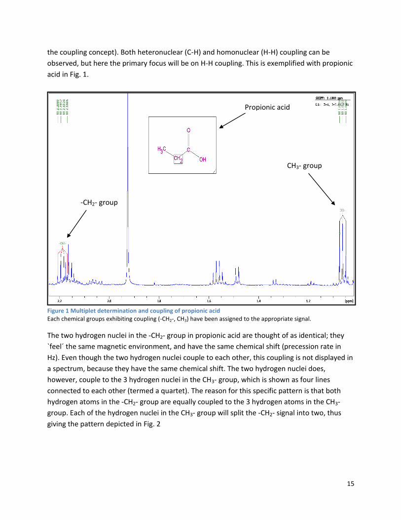
Figure 2 Splitting pattern of CH3- group
Every tier in the figure illustrates each hydrogen nuclei in the CH3- group. And every hydrogen
nuclei split the signal into two, resulting in the four lines seen in Fig. 1 for the –CH2-group. In
general, if a nucleus is equally coupled to n others, it will display (n+1) lines in a spectrum. Thus
the CH3- group is coupled to a -CH2- group, and should result in 3 (2+1) lines connected to each
other (a triplet), which is demonstrated on Fig. 1. This rule, however, is only true for S = ½, and
cannot be applied to nuclei with higher spin quantum numbers.
Another feature tied to splitting patterns is the coupling constant (termed J-constant). This
constant shows the distance between each line in the splitting pattern (in Hz). This can be
exemplified by the CH3- group in propionic acid. The J-constant is 7.68 Hz from the middle line
to the lines on each side. The reason for this symmetry is that the hydrogen nuclei are identical.
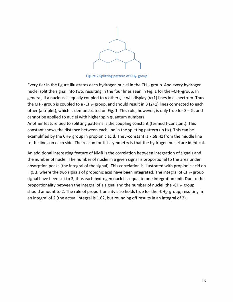
An additional interesting feature of NMR is the correlation between integration of signals and
the number of nuclei. The number of nuclei in a given signal is proportional to the area under
absorption peaks (the integral of the signal). This correlation is illustrated with propionic acid on
Fig. 3, where the two signals of propionic acid have been integrated. The integral of CH3- group
signal have been set to 3, thus each hydrogen nuclei is equal to one integration unit. Due to the
proportionality between the integral of a signal and the number of nuclei, the -CH2- group
should amount to 2. The rule of proportionality also holds true for the -CH2- group, resulting in
an integral of 2 (the actual integral is 1.62, but rounding off results in an integral of 2).
17
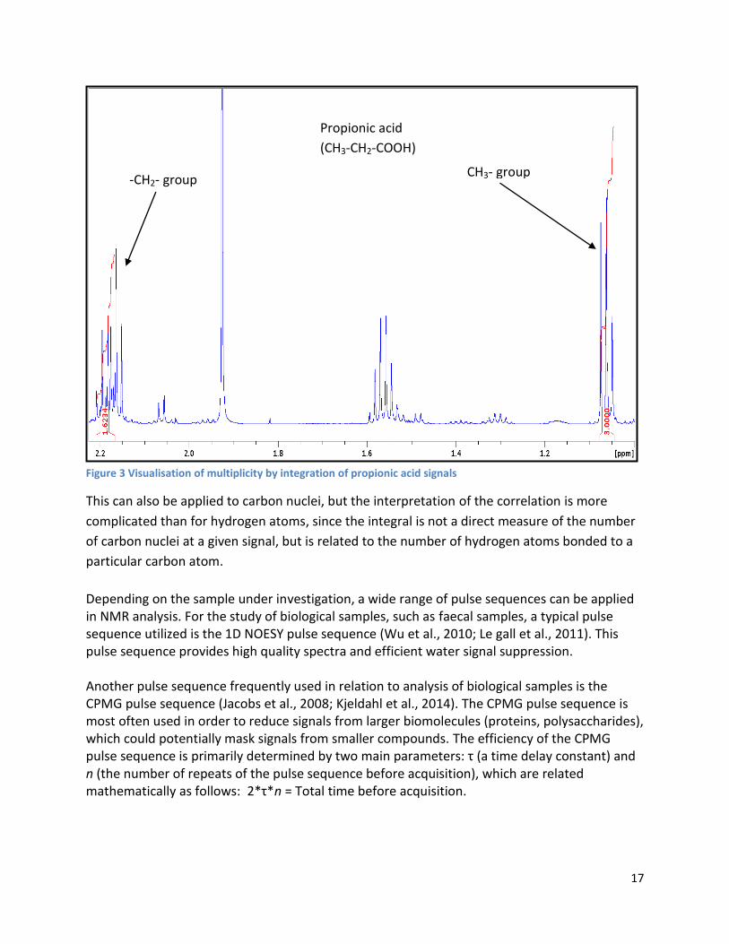
Figure 3 Visualisation of multiplicity by integration of propionic acid signals
This can also be applied to carbon nuclei, but the interpretation of the correlation is more
complicated than for hydrogen atoms, since the integral is not a direct measure of the number
of carbon nuclei at a given signal, but is related to the number of hydrogen atoms bonded to a
particular carbon atom.
Depending on the sample under investigation, a wide range of pulse sequences can be applied in NMR analysis. For the study of biological samples, such as faecal samples, a typical pulse sequence utilized is the 1D NOESY pulse sequence (Wu et al., 2010; Le gall et al., 2011). This pulse sequence provides high quality spectra and efficient water signal suppression. Another pulse sequence frequently used in relation to analysis of biological samples is the CPMG pulse sequence (Jacobs et al., 2008; Kjeldahl et al., 2014). The CPMG pulse sequence is most often used in order to reduce signals from larger biomolecules (proteins, polysaccharides), which could potentially mask signals from smaller compounds. The efficiency of the CPMG pulse sequence is primarily determined by two main parameters: τ (a time delay constant) and n (the number of repeats of the pulse sequence before acquisition), which are related mathematically as follows: 2*τ*n = Total time before acquisition.
Propionic acid
(CH3-CH2-COOH)
-CH2- group CH3- group
18
In this study, a third ubiquitously used pulse sequence, known as excitation sculpting, was also utilized in the NMR analysis. This pulse sequence is, however, not only used in biological samples, but is applied in a variety of NMR analyses.
1.9 GC
Although the methods differ markedly on the chemical and physical properties they utilize,
NMR and GC both seek to separate distinctive compounds in order to make qualitative and/or
quantitative analyses. Instead of taking advantage of the nuclear spin phenomenon as in NMR,
GC exploits the inherent differences between molecules, primarily on the basis of polarity.
The principle behind and the system setup of GC is as follows: Firstly, preparation of the sample
is needed. There is numerous ways to prepare a sample, depending on several factors, such as
ease of volatilization of a given compounds and the concentration of the compound. When a
preparation of a sample has been made, a portion of the sample is injected into the GC. On
modern GCs, an auto sampler can be connected from which samples can be automatically
injected. Otherwise, manually sample injection is required. A volume of the sample is
introduced to the system by a syringe. This syringe injects the sample volume in to a
vaporization chamber, which is heated to a relatively high temperature. Thus compounds in the
sample become volatile. An inlet of carrier gas is connected to the vaporization chamber in
order to force the volatile compounds into and through the column. Frequently, carrier gases
used are N2, H2 and He due to their reactive inertia.
The column is made of materials resistant to high temperatures, and contains a stationary
phase used for separation of the compounds in the sample. Two types of columns are often
employed: Open tubular columns, which are coated in the inside of the columns with the liquid
stationary phase. Or packed columns, in which fine particles are distributed within the column,
and coated with the liquid stationary phase. The liquid stationary phase is made up of polymers
with varying degrees of polarity, from non-polar to strongly polar.
From the vaporization chamber, the volatile compounds are forced through the column. During
the passing along the column, the compounds will interact with the stationary phase. And
depending on the polarity of the stationary phase and the polarity of the compounds, they will
interact to a greater or lesser extent. Due to this interaction, the compounds are retained in the
column for a specific period of time, after which the compounds elute from the column. Thus a
stronger interaction between the stationary phase and the compounds leads to longer
retention time.
After elution from the column, the compounds enter the detection unit attached to the GC
device. Several detection units are available, but one of the detectors most frequently used is a
flame ionization detector (FID). From the column, a flow of gas carrying the volatile compounds
19
is forced into the FID. Here it is mixed with hydrogen and air before undergoing pyrolysis,
producing a positively charged ion and an electron. The positively charged ion is collected at an
electrode, and after computation results in a signal.
During the whole process from injection and vaporization through the column to the detector,
all units are kept at a relatively high temperature to ensure that the volatile compounds are in
their gaseous state. These temperatures are often electronically controlled by a pre-
programmed temperature profiling protocol. The temperature protocol is mostly dependent on
the volatilization of the compounds under investigation (Harris, 2010; Kupiec, 2004).
2 Materials and methods
2.1 Study design
The study was designed as a double-blind, placebo-controlled trial with 2 groups (probiotic group and placebo-control group). The study period stretched over 6 months, initiated by a 4-week baseline period, followed by a 16-week treatment period and ending with a 4-week wash out period. Faecal samples were collected at 4 time points: during the 4-week baseline period, 8 weeks after baseline collection, 16 weeks after baseline collection, and during the 4-week wash out period. From these samples, faecal water content analyses and microbiological analyses were made. Furthermore, during episodes of acute diarrhoea and antibiotic therapy, additional faecal samples were collected.
2.2 Intervention supplement
The probiotic supplement was given in a dose of 1 billion (109) cells daily in a sachet. The probiotic organism used was Lactobacillus acidophilus NCFM (ATCC).
2.3 Subjects
In total, 142 subjects participated in the trial distributed as 112 elderly subjects (>65 years of
age) and 30 staff members for comparison of their pathogen and infection frequencies with
those of the elderly (18-65 years of age). The participants were recruited from elder homes in
Turku in the South Western part of Finland.
In order to determine eligibility of the study subjects, certain inclusion and exclusion criteria
were established. Subjects with no acute infection were included in the study, whereas subjects
were excluded, if antibiotics had been consumed during the preceding month, unless a regular
long-term preventive therapy was in action, which required consumption of antibiotics.
Additionally, subjects with <6 months life expectancy were also excluded. Records on past and
present diseases and medication were obtained in the baseline period and at the end of the
20
study. During the intervention, ingestion of probiotics other than the study probiotic organism
was prohibited.
In a previous study with 26 healthy elderly people, an average of log10 2.1 C. difficile cells/ g
faeces was reported. Based on this finding, it was deduced that 56 elderly subjects were
needed in order to detect a log10 difference in the quantity of C. difficile. Due to the health
status of the elderly participants and the possibility of drop-outs, an excess of 50 % subjects
was the aim during recruitment, resulting in 112 elderly subjects.
2.4 Primary outcome measure
The primary outcome was to measure the C. difficile level in faecal samples of elderly subjects. This was determined by quantitative polymerase chain reaction (qPCR), targeting a species-specific 16S rRNA gene.
2.5 Secondary outcome measures
Levels of intestinal pathogens other than C. difficile
The level of the pathogen Clostridium perfringens was also measured by qPCR.
2.6 Additional analyses
Besides the above-mentioned analyses, the qPCR method was also applied to quantify the intervention strain L. acidophilus NCFM as a quality control measure. Additionally, the genus Bifidobacterium was also quantified, since it is assumed to be a marker of health, health promoting and frequently respond to consumption of probiotics (Tiihonen et al., 2010). Volatile fatty acids (VFA) analysis was also performed and used to measure microbial activity within the intestine. Furthermore, this study also included NMR analyses. These were used for multivariate statistical analysis, comparison with the VFA analysis, and expanding the range of faecal metabolites identified in the faecal samples.
2.7 Sample collection and processing
The baseline stool samples were collected during one month. Stool samples from the subsequent time points were collected over the course of a week. The stool samples were stored frozen at -20° C at the elderly homes immediately after defecation. Once a week, the stool samples were collected and brought to a study laboratory. Here they were stored at -70 °C before shipping them to the research facilities in Kantvik, Finland. From the stool sample, minor portions were weighed out for further processing and analysis. The amounts weighed out were as follows: 0.2 g for flow cytometry; 0.2 g for DNA extraction and qPCR; 0.3 g to each microfuge tube for NMR analyses (3 x 0.3 g for lipophilic extraction and
21
3 x 0.3 for hydrophilic extraction); 0.5 g for SCFA analyses. Additional samples for NMR analyses were taken out, in order to optimise the NMR procedure.
2.8 Methods
In order to use the primary methods (qPCR, VFA and NMR), several preparatory methods had to be performed. The following paragraph describes the methods used, both the preparatory phases and the primary methods. Low amounts of faeces in stools necessitated a priority ranking of analysis in the following order: DNA extraction (for qPCR) > NMR > VFA The priority order was made according to the primary outcomes of the study, and the expected outcomes of the master thesis.
2.9 Total Bacterial Count
2.9.1 Preparatory phase
For the Total Bacterial Count, Tween wash buffer (50 mM sodium phosphate pH 8, 0.1 % Tween 80) was added in a ratio of 1 unit faeces to 30 units wash buffer. Afterwards, the tube was vortex-mixed thoroughly to detach the faeces from the tube, and suspend it in the buffer. This was followed by shaking at 200 rpm for 10 min. at room temperature, and centrifugation at 200xg for 15 min. at 20° C. Lastly, the liquid phase was carefully transferred to collection tubes, in order to avoid accompanying transfer of solid faeces particles. The last steps (shaking, centrifugation and liquid transfer) was done 3 times to ensure that the faeces sample had been adequately washed, and as many bacterial cells as possible had been suspended in the liquid sample. Subsequently, 890 µL of liquid sample was transferred to a microfuge tube containing 110 µL 36% formaldehyde. During the washing, the collection tubes were kept on ice, and the final samples were stored at 4 °C.
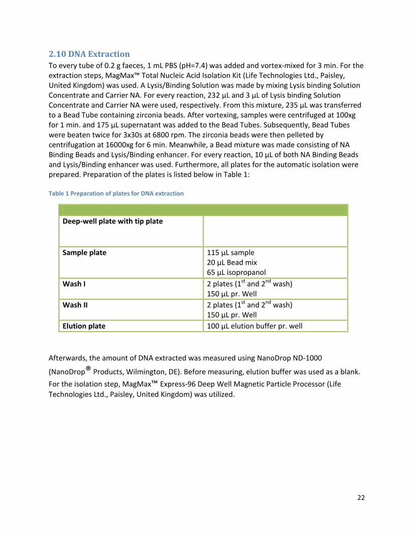
22
2.10 DNA Extraction
To every tube of 0.2 g faeces, 1 mL PBS (pH=7.4) was added and vortex-mixed for 3 min. For the extraction steps, MagMax™ Total Nucleic Acid Isolation Kit (Life Technologies Ltd., Paisley, United Kingdom) was used. A Lysis/Binding Solution was made by mixing Lysis binding Solution Concentrate and Carrier NA. For every reaction, 232 µL and 3 µL of Lysis binding Solution Concentrate and Carrier NA were used, respectively. From this mixture, 235 µL was transferred to a Bead Tube containing zirconia beads. After vortexing, samples were centrifuged at 100xg for 1 min. and 175 µL supernatant was added to the Bead Tubes. Subsequently, Bead Tubes were beaten twice for 3x30s at 6800 rpm. The zirconia beads were then pelleted by centrifugation at 16000xg for 6 min. Meanwhile, a Bead mixture was made consisting of NA Binding Beads and Lysis/Binding enhancer. For every reaction, 10 µL of both NA Binding Beads and Lysis/Binding enhancer was used. Furthermore, all plates for the automatic isolation were prepared. Preparation of the plates is listed below in Table 1: Table 1 Preparation of plates for DNA extraction
Deep-well plate with tip plate
Sample plate 115 µL sample 20 µL Bead mix 65 µL isopropanol
Wash I 2 plates (1st and 2nd wash) 150 µL pr. Well
Wash II 2 plates (1st and 2nd wash) 150 µL pr. Well
Elution plate 100 µL elution buffer pr. well
Afterwards, the amount of DNA extracted was measured using NanoDrop ND-1000
(NanoDrop® Products, Wilmington, DE). Before measuring, elution buffer was used as a blank.
For the isolation step, MagMax™ Express-96 Deep Well Magnetic Particle Processor (Life
Technologies Ltd., Paisley, United Kingdom) was utilized.
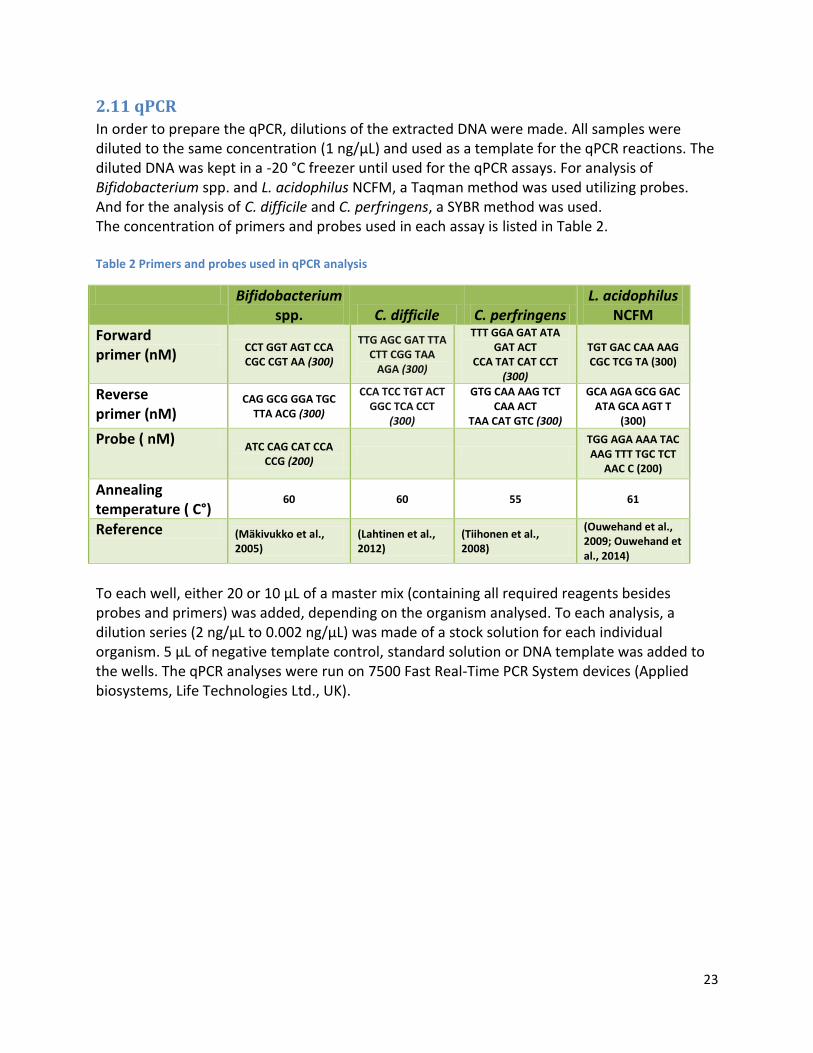
23
2.11 qPCR
In order to prepare the qPCR, dilutions of the extracted DNA were made. All samples were diluted to the same concentration (1 ng/µL) and used as a template for the qPCR reactions. The diluted DNA was kept in a -20 °C freezer until used for the qPCR assays. For analysis of Bifidobacterium spp. and L. acidophilus NCFM, a Taqman method was used utilizing probes. And for the analysis of C. difficile and C. perfringens, a SYBR method was used. The concentration of primers and probes used in each assay is listed in Table 2. Table 2 Primers and probes used in qPCR analysis
Bifidobacterium spp. C. difficile C. perfringens
L. acidophilus NCFM
Forward primer (nM)
CCT GGT AGT CCA CGC CGT AA (300)
TTG AGC GAT TTA CTT CGG TAA
AGA (300)
TTT GGA GAT ATA GAT ACT
CCA TAT CAT CCT (300)
TGT GAC CAA AAG CGC TCG TA (300)
Reverse primer (nM)
CAG GCG GGA TGC TTA ACG (300)
CCA TCC TGT ACT GGC TCA CCT
(300)
GTG CAA AAG TCT CAA ACT
TAA CAT GTC (300)
GCA AGA GCG GAC ATA GCA AGT T
(300)
Probe ( nM) ATC CAG CAT CCA
CCG (200)
TGG AGA AAA TAC AAG TTT TGC TCT
AAC C (200)
Annealing temperature ( C°)
60 60 55 61
Reference (Mäkivukko et al., 2005)
(Lahtinen et al., 2012)
(Tiihonen et al., 2008)
(Ouwehand et al., 2009; Ouwehand et al., 2014)
To each well, either 20 or 10 µL of a master mix (containing all required reagents besides probes and primers) was added, depending on the organism analysed. To each analysis, a dilution series (2 ng/µL to 0.002 ng/µL) was made of a stock solution for each individual organism. 5 µL of negative template control, standard solution or DNA template was added to the wells. The qPCR analyses were run on 7500 Fast Real-Time PCR System devices (Applied biosystems, Life Technologies Ltd., UK).
24
2.12 VFA Analysis
For the VFA analysis by GC, 0.5 mL internal standard (ISTD) solution (20 mM pivalic acid), and 4 mL of ion exchanged water was added to the tubes. The tubes were shaken for 5 min. in a cold room at +4°C, and centrifuged at 7000 RPM for 10 min. at 10 °C. Supernatant was mixed in a 2:1 ratio with a saturated oxalic acid solution, and left in a cold room at 4 °C for 60 min. Samples were then centrifuged for 3 min. at 16000 x g, and the supernatant was transferred to glass vials, and placed on the GC auto sampler. For the analysis, a glass column packed with 80/120 Carbopack B-DA/4% Carbowax 20 M stationary phase (2m x 2mm, Supelco, Bellefonte PA, USA) was used. The temperature of the column was 175 °C during the analysis, and helium was utilised as a carrier gas at a flow rate of 24 mL/min. From the sample, 1 microliter was injected onto the column. The temperatures of the injector and flame ionisation detector were 200 °C and 245 °C, respectively (modified after Ouwehand et al., 2009). Volatile fatty acid standard (VFA STD) vials were also prepared. The VFA STD contained acetic acid, propionic acid, isobutyric acid, butyric acid, 2-methylbutyric acid, isovaleric acid, lactic acid, valeric acid and pivalic acid. Each acid had been weighed off into a 200 mL measuring flask, to which water was added. Subsequently, the concentrations of the acids were calculated. Two VFA STD-vials were prepared by adding 500 µL of VFA STD and 250 µL saturated oxalic acid to the vials. A Hewlett-Packard HP 6890 GC system (Agilent technologies Inc., CA, USA) was used for the GC analysis, on which an Agilent Technologies 7693A Automatic liquid sampler (Agilent Technologies Inc., CA, USA) had been attached. A protocol was made in the program belonging to the GC system for the analysis.
25
2.13 NMR
For the NMR analysis, several tests were performed to obtain NMR spectra of an adequate, acceptable quality. Simultaneously, a multi sample handling system was tested to ease the preparation of samples. After testing, NMR analyses of the complete sampling set were conducted.
2.13.1 Pre-analysis phase
In the testing phase, a numbers of procedures and methods were investigated. In the tests, where a phosphate buffered saline (PBS) buffer was used as solvent, a buffer containing the following reagents was prepared: NaCl (150 mM), NaH2PO4 ∙ 1 H2O and Na2HPO4 ∙ 12 H2O (total concentration 100 mM), NaN3 (sodium azide, 2 mM), 3-(trimethylsilyl)-2,2′,3,3′-tetradeuteropropanoic acid sodium salt (TSP) (0.1 %, w/v), D2O (10 %, v/v). All constituents were solubilised in purified water (Millipore-q). Some tests used a phosphate buffer (PB) as solvent, comprised of the same constituents as the PBS buffer, except for NaCl.
2.13.1.1 Deuterated water extraction:
100 mg faecal sample was transferred to a microfuge tube to which 600 µL D2O was added. The tube was then vortex-mixed at 3000 RPM for 45 s at room temperature (RT) and centrifuged at 10000xg for 10 min. at 5 °C. This was followed by transferring of 550 µL of the supernatant to an NMR tube.
2.13.1.2 Deuterated water and methanol extraction (with NaOH and formic acid):
2 x 100 mg faecal sample was weighed off into microfuge tubes to which 200 µL NaOH (0.15 M) and 200 µL purified water. In addition, 200 µL of formic acid was added to one of the tubes. After brief mixing, the solutions were freeze-dried. Subsequently, 600 µL D2O was added to the tubes, which were then vortex-mixed for 2 x 45 s at 3000 RPM at RT and centrifuged at 10000xg for 10 min. at 5 °C. From the tubes, 550 µL of the supernatants was transferred to NMR tubes. The same procedure was done for methanol extraction, except the re-solubilisation step, in which deuterated methanol (CD3OD) was used instead of deuterated water. Additional testing of faecal samples solubilised with NaOH was done. The same procedure was used as described above, but formic acid was omitted and pH was measured.
2.13.1.3 Phosphate buffered saline (PBS) buffer extraction
50 mg faecal sample was dissolved in 600 µL PBS buffer in purified water. The buffer contained D2O for NMR locking as well as NaN3 for inhibition of bacterial growth and TSP as a zero reference. The solubilised sample was then vortex-mixed for 45 s at 3000 RPM at RT and centrifuged. Subsequently, 550 µL of the supernatant was transferred to an NMR tube.

26
2.13.1.4 Testing of NMR pulse sequence
A test of the NMR sequences utilized was also done. The spectra produced in the sections described above were run with the ZGESGP sequence. In the following, a test between the ZGESGP sequence and the CPMG sequence was made in order to compare the spectra obtained by the individual procedure. 2 x 50 mg faecal sample was weighed out into microfuge tubes. To each microfuge tube 600 µL PBS buffer was added, followed by vortex-mixing and centrifugation. Afterwards, 550 µL of the supernatants was transferred to NMR tubes. One tube was run on the ZGESGP sequence and the other run on the CPMG sequence.
2.13.1.5 Test of mixing duration
The purpose of the mixing duration testing was to examine, if mild mixing was sufficient to extract a decent amount of compounds for the NMR analysis, or if thorough mixing would provide better spectra. For the testing of mixing duration, 2 x 50 mg faecal samples were weighed off into microfuge tubes. To each tube, 600 µL PBS buffer was added. Then one tube was vortex-mixed and hand-centrifuged for five rounds (45 s. vortex-mixing at 3000 RPM at RT, and hand centrifugation for 20 s. each round), and the other was vortex-mixed and hand-centrifuged for one round. Subsequently, both tubes were briefly vortex-mixed and centrifuged for 10 min. at 5 °C at 10000xg, followed by transferring 550 µL of the supernatants to NMR tubes.
2.13.1.6 Sonication and extraction cycles of faecal samples
Four samples were needed for sonication and extraction testing: 1 for one extraction cycle without sonication, 1 for one extraction cycle with sonication, 1 for two extraction cycles without sonication, 1 for two extraction cycles with sonication. The procedure was as follows: 4 x 100 mg faecal sample was weighed out and transferred to microfuge tubes. To each tube, 700 µL PBS buffer was added followed by vortex-mixing and hand centrifugation (vortex-mixing for 45 s. at 3000 RPM and hand centrifugation for 20 s. each round) for five rounds. Subsequently, two tubes were placed in a water bath and sonicated for 10 min., after which all tubes were centrifuged at 5° C for 10 min. at 10.000xg. For two tubes (with and without sonication), the supernatants were transferred to new microfuge tubes. The two other tubes with and without sonication was then used for a repeat of the procedure (except sonication). After these tubes were centrifuged at 5° C for 10 min. at 10.000xg, the supernatants were added to the tubes containing the supernatants from the first extraction. The tubes containing the pooled samples were then centrifuged at 5° C for 10 min. at 14.000xg. This was followed by transferring of 550 µL of the supernatants to NMR tubes from both sonicated and non-sonicated tubes (1 extraction round), as well as sonicated and non-sonicated tubes (2 extraction rounds).
27
2.13.1.7 Sample weight optimization
For sample weight optimization test, 5 x faecal samples were weighed out into microfuge tubes. The weight of the samples was as follows: 5,0 mg; 9,1 mg; 9,6 mg; 19,2 mg; 38,4 mg; 149,9 mg, thus providing a sample weight dilution series. To each microfuge tube, 700 µL PBS buffer was added followed by vortex-mixing and hand centrifugation (vortex-mixing for 45 s. at 3000 RPM and hand centrifugation for 20 s. each round) for five rounds. Subsequently, the tubes were centrifuged at 5° C for 10 min. At 10.000xg, and 550 µL of the supernatants was transferred to NMR tubes.
2.13.1.8 Volume-to-sample ratio
From the same sample tube, 5 x 40 mg was weighed out and transferred to new microfuge tubes. PBS buffer was added to the microfuge tubes in the following amounts: 700 µL (two tubes), 1400 µL (two tubes), and 2100 µL (one tube). Following the addition of buffer, the tubes were vortex-mixed and hand centrifuged (vortex-mixing for 45 s. at 3000 RPM and hand centrifugation for 20 s. each round) for five rounds. Afterwards, the tubes were centrifuged at 5° C for 10 min. at 10.000xg, followed by transferring of 550 µL of the supernatants to NMR tubes.
2.13.1.9 Filtration and acid mix spiking of faecal samples
For the testing of filtration and acid mix spiking, 2 samples were made: One without filtration and acid mixture added and one with filtration and acid mixture. The acid mix contained the following compounds: Acetic acid, propionic acid, butyric acid, isobutyric acid, 2-methylbutyric acid, isovaleric acid, lactic acid, valeric acid, D/L-3-phenyllactic acid, and phenyl acetate. The procedure was as follows: 2x40 mg was weighed out into new microfuge tubes. To these tubes, PBS buffer and a portion of the acid mixture was added to give a total volume of 700 µL. This was followed by vortex-mixing and hand centrifugation (vortex-mixing for 45 s. at 3000 RPM and hand centrifugation for 20 s. each round) for five rounds. Subsequently, 350 µL of the sample slurry from one of the tubes was transferred to a pre-washed filtration tube (molecular weight filter, cut-off: 10 kDa). The tube was then centrifuged at 5° C for 10 min. at 14.000xg. Another 350 µL of the sample slurry was transferred to the filtration tube, and the centrifugation was repeated. Afterwards, the pooled filtrate was transferred to a new microfuge tube and centrifuged at 5° C for 10 min. at 10.000xg. The same procedure (vortex-mixing and centrifugation) was applied to the other tube with omission of the filtration step. After centrifugation of the samples, 550 µL of the supernatant was transferred to NMR tubes.
28
2.13.1.10 Biphasic extraction with acid mix spiking of lyophilized faeces
For the biphasic extraction, 2 samples were prepared: one sample with acid mix spiked in and one without acid mix spiked in. The acid mix contained the following compounds: Acetic acid, propionic acid, butyric acid, isobutyric acid, 2-methylbutyric acid, isovaleric acid, lactic acid, valeric acid, D/L-3-phenyllactic acid, and phenyl acetate. The procedure was as follows: 2 faecal samples were lyophilized with subsequent weighing out of 20 mg from each lyophilized sample into new microfuge tubes. Before usage, the solvents (methanol, chloroform and water) had been pre-cooled by storage on ice. To each microfuge tube, 300 µL of each solvent was added one at a time, separated by thorough vortex-mixing and 10 min. of storage on ice. With each of the solvents, a portion of the acid mixture was added. After the last solvent had been added, the tubes were stored in a refrigerator at 4° C over night to obtain phase separation. The next day, the samples were centrifuged for 30 min. at 1.400xg at 4° C. This was followed by transferring of the upper methanol-water phase and the lower chloroform phase to individual microfuge tubes. Afterwards, the methanol-water tube and the chloroform tube were freeze-dried for 3 hours and 1 hour, respectively. Subsequently, the methanol-water extracts were re-dissolved in 575 µL D2O with TSP and H2O. The chloroform extracts were re-dissolved in 575 µL CHCl3-d with TMS. This produced four tubes for NMR analysis: Chloroform extracts with or without acid mix added, and methanol-water extracts with or without acid mix added. All tubes were briefly vortex-mixed, followed by transferring of 550 µL of the solution to NMR tubes. Simultaneously, a sample for methanol extraction was prepared as follows for comparison: 20 mg lyophilized sample was weighed off into a new microfuge tube, and dissolved in 700 µL CD3OD. This was followed by vortex-mixing and hand centrifugation (vortex-mixing for 45 s. at 3000 RPM and hand centrifugation for 20 s. each round) for five rounds with subsequent centrifugation at 5° C for 10 min. at 10.000xg. From the supernatant, 550 µL was transferred to an NMR tube to which 4 µL CD3OD with TSP was added.
2.13.1.11 Optimization of NMR pulse sequence
Optimization of the preferred NMR pulse sequence (CPMG) was performed. However, a new CPMG optimization was set up with new ranges of values for each parameter, based on settings in literature. In brief, the experiment was prepared as follows: 40 mg faecal sample was weighed out into a microfuge tube to which 700 µL PBS buffer was added. The tube was then vortex-mixed and hand centrifuged (vortex-mixing for 45 s. at 3000 RPM and hand centrifugation for 20 s. each round) for five rounds, followed by centrifugation at 5° C for 10 min. at 10.000xg. This was followed by transferring of 550 µL supernatant to an NMR tube. The CPMG optimization was then executed as two individual step by step experiments, consisting of 10 analyses in which the first parameter was held constant at a specific level and the second parameter was gradually increased.
29
2.13.1.12 Testing of solubilisation method
A new solubilisation method was tested and prepared as follows: one mL PBS buffer was added to 300 mg faecal sample. The solution was thoroughly vortex-mixed and made into slurry, followed by brief hand centrifugation. A volume equal to 40 mg faecal material was transferred from the slurry solution to a new microfuge tube. PBS buffer was added to the microfuge tube to reach a total volume of 700 µL. The tube was then vortex-mixed and hand centrifuged (vortex-mixing for 45 s. at 3000 RPM and hand centrifugation for 20 s. each round) for five rounds, followed by centrifugation at 5° C for 10 min. at 10.000xg. This was followed by transferring of 550 µL supernatant to an NMR tube. From the same sample, a methanol extraction was also tested. A volume equal to 40 mg was transferred from the slurry described above to a new microfuge tube. Subsequently, the sample was freeze-dried, re-dissolved in 700 µL deuterated methanol and vortex-mixed and hand centrifuged (vortex-mixing for 45 s. at 3000 RPM and hand centrifugation for 20 s. each round) for five rounds, followed by centrifugation at 5° C for 10 min. at 10.000xg. This was followed by transferring of 550 µL supernatant to an NMR tube.
2.13.1.13 Testing of NH4Cl addition
Addition of NH4Cl in the preparation of samples was tested. This was investigated in several experiments, where the final concentrations of NH4Cl ranged from 673 mM to 60 mM. The samples for these experiments were prepared as follows: one mL PBS buffer was added to 300 mg faecal sample. The solution was vortex-mixed (3000 RPM for 2-3 min. at RT, 1400 RPM for 9 min. at 6-8° C) with subsequent centrifugation (8000xg for 1 min. at 5° C). This was followed by transferring of a volume equal to 40 mg faecal material to a new microfuge tube to which PBS buffer was added reaching a final volume of 700 μL. The tube was then vortex-mixed (1400 RPM at 6-8° C for 5 min.) and centrifuged (14000xg at 5° C for 10 min.), followed by transferring of 550 μL supernatant to a NMR tube. In these experiments, the testing of exclusion of NaCl from the buffer used was also investigated.
30
2.13.1.14 Testing of pulse sequence, addition of NH4Cl, and dilution of samples
In this series of experiments, testing of pulse sequences, addition of NH4Cl to buffer, and sample dilution was investigated. The samples were prepared as follows: the first sample (≈300 mg) was solubilised in 1 mL PBS buffer with NH4Cl, followed by vortex-mixing (3000 RPM for 3 min. at RT, 1400 RPM for 9 min. at 7° C) and centrifugation (8000xg for 1 min. at 5° C). Subsequently, 2 x 280 μL supernatant was transferred to two microfuge tubes, to which either PBS buffer with NH4Cl or PBS without NH4Cl was added, resulting in a total volume of 700 μL. Subsequently, the tubes were vortex-mixed (1400 RPM at 7° C for 5 min.) and centrifuged (14000xg for 10 min. at 5° C), after which 2 x 550 μL was transferred to two NMR-tubes; one for CPMG analysis and one for ZGESGP analysis. A second sample (≈300 mg) was solubilised in 1 mL PBS buffer, vortex-mixed (3000 RPM for 3 min. at RT, 1400 RPM for 9 min. at 7° C) and centrifuged (25000xg for 10 min. at 5° C). This was followed by transferring of 550 μL supernatant to a NMR tube. The last sample (≈300 mg) was solubilised in 1 mL PB (phosphate buffer) without NaCl, vortex-mixed (3000 RPM for 3 min. at RT, 1400 RPM for 9 min. at 7° C) and centrifuged (8000xg for 1 min. at 5° C). From the supernatant, 2 x 280 μL was taken to two new microfuge tubes, to which PB with or without NH4Cl was added up to a total volume of 700 μL. Both tubes were vortex-mixed and centrifuged similarly to the PBS solubilised samples. And after centrifugation, 2 x 550 μL was transferred to 2 NMR tubes; one for CPMG analysis and one for ZGESGP analysis.
2.13.1.15 Testing of solvent and pulse sequence
Combinations of different solvent and pulse sequences were also tested. The samples were prepared as previously described. Briefly, 3 samples (≈3x300 mg) were solubilised in 1 mL PBS buffer, 1 mL D2O or 1 mL phosphate buffer (PB). This was followed by vortex-mixing (3000 RPM for 3 min. at RT, 1400 RPM for 9 min. at 7° C) and centrifugation (8000xg for 1 min. at 5° C) with subsequent transferring of 3 x 280 μL of the supernatant to three microfuge tubes. To each tube, solvent was added according to the solubilisation step, reaching a total volume of 700 μL in each tube. Afterwards, the tubes were vortex-mixed (1400 RPM at 7° C for 5 min.) and centrifuged (14000xg for 10 min. at 5° C), and from the supernatant 3 x 550 μL was transferred to NMR-tubes. The samples were then analysed with the modified CPMG pulse sequence (described earlier), as well as the ZGESGP pulse sequence.
2.13.1.16 Additional testing of pulse sequences, sample dilution and preparation procedure
In continuation of the tests described above, additional pulse sequences and preparation procedure comparisons were conducted. For these comparisons, 3 samples were used. These were prepared as follows: The first sample (≈300 mg) was solubilised in 1 mL PB. The other two samples were also solubilised in PB, but in a 1:2, wfeces: vbuffer ratio. The first sample was vortex-mixed (3 min. at RT at 3000 RPM) and centrifuged (20000xg for 10 min. at 5° C). From the supernatant, 550 μL was transferred to a NMR tube. One of the other samples was vortex-mixed (3000 RPM for 2 min. at RT, 1400 RPM for 9 min. at 10° C) and centrifuged (8000xg for 1 min. at 5° C), after which 280 μL of the supernatant was transferred to a new microfuge tube. To this tube, PB was added to reach a final volume of 700
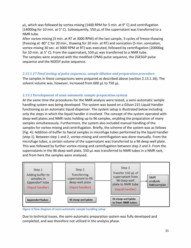
31
μL, which was followed by vortex-mixing (1400 RPM for 5 min. at 9° C) and centrifugation (14000xg for 10 min. at 5° C). Subsequently, 550 μL of the supernatant was transferred to a NMR tube. After vortex-mixing (3 min. at RT at 3000 RPM) of the last sample, 3 cycles of freeze-thawing (freezing at -80° C for 20 min., thawing for 20 min. at RT) and sonication (5 min. sonication, vortex-mixing 30 sec. at 3000 RPM at RT) was executed, followed by centrifugation (20000xg for 10 min. at 5° C). From the supernatant, 550 μL was transferred to a NMR tube. The samples were analysed with the modified CPMG pulse sequence, the ZGESGP pulse sequence and the NOESY pulse sequence.
2.13.1.17 Final testing of pulse sequences, sample dilution and preparation procedure
The samples in these comparisons were prepared as described above (section 2.13.1.16). The solvent volume was, however, increased from 600 μL to 750 μL.
2.13.2 Development of semi-automatic sample preparation system
At the same time the procedures for the NMR analysis were tested, a semi-automatic sample handling system was being developed. The system was based on a Gilson 215 Liquid Handler functioning as an automatic liquid dispenser. The system setup is illustrated below including only the steps in which the liquid handler is involved. The concept of the system operated with deep-well plates and NMR racks holding up to 96 samples, enabling the preparation of many samples simultaneously. Furthermore, the system also included manual handling of the samples for vortex-mixing and centrifugation. Briefly, the scheme of the system was as follows (Fig. 4): Addition of buffer to faecal samples in microfuge tubes performed by the liquid handler (step 1). Between step 1 and 2, vortex-mixing and centrifugation was done manually. From the microfuge tubes, a certain volume of the supernatant was transferred to a 96 deep-well plate. This was followed by further vortex-mixing and centrifugation between step 2 and 3. From the supernatants in the 96 deep-well plate, 550 µL was transferred to NMR tubes in a NMR rack, and from here the samples were analysed.
Figure 4 Flow diagram of semi-automatic sample handling setup
Due to technical issues, the semi-automatic preparation system was fully developed and completed, and was therefore not utilized in the analysis phase.
32
2.13.3 Analysis phase
2.13.3.1 Data Acquisition
After all testing had been completed, a sample preparation procedure and pulse sequence was chosen for the analysis of the complete sampling set. All samples were then prepared as follows: 750 μL PB (NaH2PO4 ∙ 1 H2O (42 mM), Na2HPO4 ∙ 12 H2O (58 mM), TSP (0.1 %, w/v), D2O (10 %, v/v), NaN3 (2 mM), all in purified water (Milipore-q); pH=7.02) was added to 300 mg faecal sample with subsequent thorough vortex-mixing (3000 RPM for 3 min. at RT) and centrifugation (20000xg for 10 min. at 5° C). This was followed by transferring of 550 µL supernatant to a NMR tube. All 1H NMR spectra were acquired (including the pre-analysis tests) with a Bruker Avance III 600 MHz NMR spectrometer (Bruker Biospin, Germany) equipped with a 5.0 mm BBO probe, operating at a proton NMR frequency of 600.13 MHz. Furthermore, a SampleJet auto sampler (Bruker Biospin, Germany) was attached to the spectrometer, in which samples were cooled to 5-7 °C. The spectra were obtained with a CPMG pulse sequence (D-90°-(τ-180°-τ)n-FID) including a presaturation step to suppress the water signal. The spin-echo loop time (2∙τ∙n) was adjusted to 466 ms (milliseconds), and 128 scans (NS) were acquired for each sample. The acquisition parameters included 32k data points, a spectral width (SW) of 7212 Hz, acquisition time (AQ) of 2.27 s and a relaxation delay (D) of 3 s. The analysis time for each sample was estimated to ≈12 min. excluding pre-heating time (4 min.) of samples between each analysis, resulting in an actual analysis time of ≈16 min. for each sample. Additionally, a line broadening factor (LB) of 0.3 Hz was applied to the spectra. From each of the initial 72 samples prepared, 90 µL was transferred to a 15 mL tube and divided into aliquots. These served as pooled control samples in the subsequent runs to test if systematic errors would occur. In addition, each run also included two blank samples (buffer) to test if signals found in the spectra would develop due to signal(s) from the solvent.
2.13.3.2 Data pre-processing and compound identification
After the generation of the NMR spectra from the analysis phase, all spectra were manually phase adjusted and baseline corrected, and calibrated to TSP set at 0.0 ppm using TOPSPIN (version 3.0, Bruker Biospin, Germany). Subsequently, spectra identification of compounds was initiated. This was done by using findings in the literature, as well as using the AMIX package (version 3.9.9, Bruker Biospin, Germany) to make spectral overlay comparisons provided by the spectral database (SBASE) included in the AMIX package. Additionally, metabolomics websites were also used in the identification process, primarily the Human Metabolome Database (HMDB) (www.HMDB.ca) and Biological Magnetic Resonance Data Bank (BMRB) (www.BMRB.wisc.edu/metabolomics).
33
2.13.4 Statistical analysis
Before the statistical analysis, the qPCR data had been log10 transformed.
For statistical analysis of the qPCR and GC data, a general linear model was setup. The model is
mathematically formulated as follows:
Yijk = µ + αj + βk + (αβ)jk + bi(j) + eijk
Here, yijk is log(count) for subject i and treatment j at time k. Furthermore, µ is the fixed
intercept, αj is the fixed main effect for treatment (study group), βk is the fixed main effect for
time (time point), (αβ)jk is the fixed interaction between treatment and time, and bi(j) is the
random effect of subject (ID(Study_group)) modelled by independent and identically
distributed normal distributions and eijk is the residual error of independent and identically
distributed normal distributions, also independent of the random subjects.
In this study, time is regarded as a categorical variable with 4 levels: time point A, time point B,
time point C, and time point D. In addition, the subjects have been nested into treatments as a
random term (bi(j)), indicated by the parenthesis around subscript j.
Only multifactor analysis of variance (ANOVA) was used for interpretation of data.
Furthermore, the interaction plots shown in the qPCR results section have been mean centred
with respect to time point A to better visualise the difference between each time point. This is
based on the premise that at time point A (time zero before treatment), the subjects
participating in this study have been randomly sampled and represent a larger population, in
which the level of a specific bacterium is assumed to be the same for all individuals.
Furthermore, it should be noted that a partial blinding to the study was still in effect during the statistical analysis to avoid statistical bias. On basis of the partial blinding, the two study groups have been designated the letters A and B in the results section.
34
The data for the statistical analysis was selected, based on the criteria listed below in Table 3, which also include subtraction of the negative template control. The negative template control contains no DNA template, thus no amplification should be observed. If amplification was seen, it was considered background noise, and therefore subtracted from the replicate values.
Table 3 Selection criteria for data used in the statistical analysis
Replicate – negative template control = negative result => Data treated as a zero
measurement (0) in the statistical analysis
Rep. 1 (not detected), rep. 2 (not detected), rep. 3 (not detected) => Data for that
sample treated as Not detected (blank)
Rep. 1 (detected), rep. 2 (not detected), rep. 3 (not detected) => Data used for
statistical analysis
Rep. 1 (detected), rep. 2 (detected), rep. 3 (not detected) => Data from mean quantity
of two replicates used for statistical analysis
Rep. 1 (detected), rep. 2 (detected), rep. 3 (detected) => Data from mean quantity of
three replicates used for statistical analysis
Furthermore, all samples were run in triplicates. All data was included in the statistical analysis,
also samples with results for only 1 replicate. Extremely low measurements resulted in negative
values, when log10 transformed, but were still included in the statistical analysis. These were
included since they still counts as actually measurements, and should be included in the
statistical analysis. The mean quantity was used for log10 calculations, based on either 2 or 3
replicates.
Table 4 Alternative approach for data selection
ND = <2 replicate measurements
Detection of bacteria > 5 cycles after lowest standard concentration threshold cycle
(Ct) => Qualitative consideration (positive or negative)
Another approach to data selection is given above in Table 4. These selection criteria take on a
more conservative approach, including only data from minimum two replicates and consider
measurements 5 Ct after the lowest standard concentration as qualitative, and not
quantitative. However, the alternative approach leads to inclusion of 29 measurements in the
statistical analysis, whereas 192 measurements were included in the data selection approach
used in this thesis. This is one of the reasons data selection was based on the criteria in Table 4.
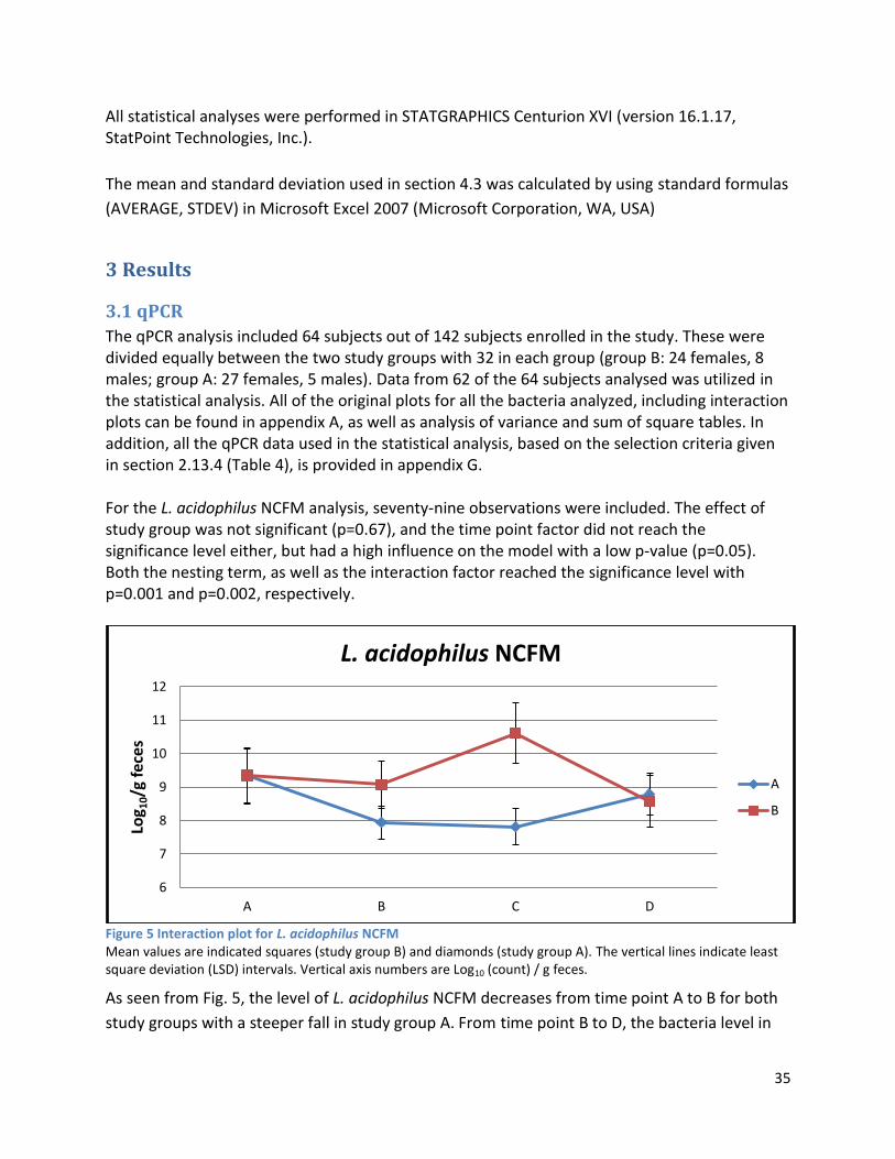
35
All statistical analyses were performed in STATGRAPHICS Centurion XVI (version 16.1.17, StatPoint Technologies, Inc.).
The mean and standard deviation used in section 4.3 was calculated by using standard formulas
(AVERAGE, STDEV) in Microsoft Excel 2007 (Microsoft Corporation, WA, USA)
3 Results
3.1 qPCR
The qPCR analysis included 64 subjects out of 142 subjects enrolled in the study. These were divided equally between the two study groups with 32 in each group (group B: 24 females, 8 males; group A: 27 females, 5 males). Data from 62 of the 64 subjects analysed was utilized in the statistical analysis. All of the original plots for all the bacteria analyzed, including interaction plots can be found in appendix A, as well as analysis of variance and sum of square tables. In addition, all the qPCR data used in the statistical analysis, based on the selection criteria given in section 2.13.4 (Table 4), is provided in appendix G. For the L. acidophilus NCFM analysis, seventy-nine observations were included. The effect of study group was not significant (p=0.67), and the time point factor did not reach the significance level either, but had a high influence on the model with a low p-value (p=0.05). Both the nesting term, as well as the interaction factor reached the significance level with p=0.001 and p=0.002, respectively.
Figure 5 Interaction plot for L. acidophilus NCFM Mean values are indicated squares (study group B) and diamonds (study group A). The vertical lines indicate least square deviation (LSD) intervals. Vertical axis numbers are Log10 (count) / g feces.
As seen from Fig. 5, the level of L. acidophilus NCFM decreases from time point A to B for both
study groups with a steeper fall in study group A. From time point B to D, the bacteria level in
6
7
8
9
10
11
12
A B C D
Log 1
0/g
fec
es
L. acidophilus NCFM
A
B
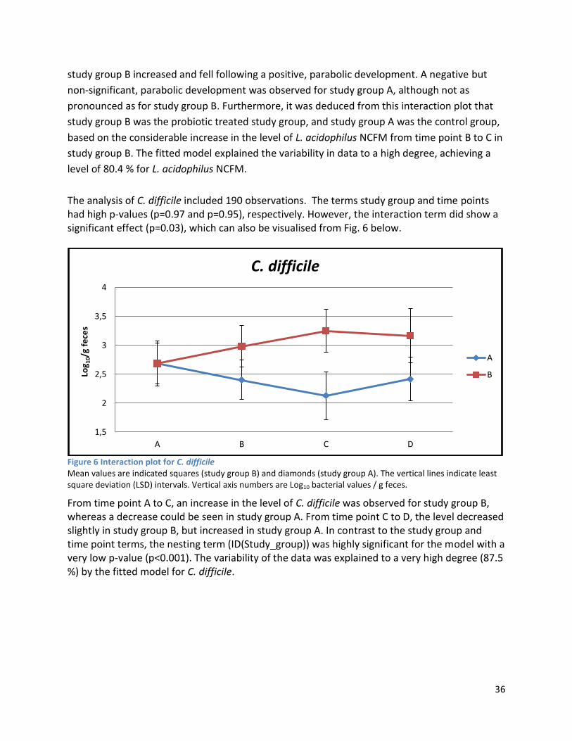
36
study group B increased and fell following a positive, parabolic development. A negative but
non-significant, parabolic development was observed for study group A, although not as
pronounced as for study group B. Furthermore, it was deduced from this interaction plot that
study group B was the probiotic treated study group, and study group A was the control group,
based on the considerable increase in the level of L. acidophilus NCFM from time point B to C in
study group B. The fitted model explained the variability in data to a high degree, achieving a
level of 80.4 % for L. acidophilus NCFM.
The analysis of C. difficile included 190 observations. The terms study group and time points had high p-values (p=0.97 and p=0.95), respectively. However, the interaction term did show a significant effect (p=0.03), which can also be visualised from Fig. 6 below.
Figure 6 Interaction plot for C. difficile Mean values are indicated squares (study group B) and diamonds (study group A). The vertical lines indicate least square deviation (LSD) intervals. Vertical axis numbers are Log10 bacterial values / g feces.
From time point A to C, an increase in the level of C. difficile was observed for study group B, whereas a decrease could be seen in study group A. From time point C to D, the level decreased slightly in study group B, but increased in study group A. In contrast to the study group and time point terms, the nesting term (ID(Study_group)) was highly significant for the model with a very low p-value (p<0.001). The variability of the data was explained to a very high degree (87.5 %) by the fitted model for C. difficile.
1,5
2
2,5
3
3,5
4
A B C D
Log 1
0/g
fece
s
C. difficile
A
B
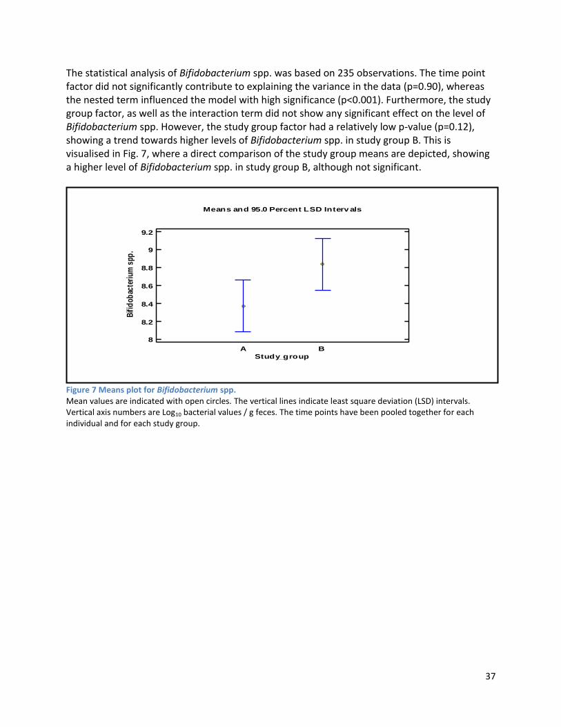
37
The statistical analysis of Bifidobacterium spp. was based on 235 observations. The time point factor did not significantly contribute to explaining the variance in the data (p=0.90), whereas the nested term influenced the model with high significance (p<0.001). Furthermore, the study group factor, as well as the interaction term did not show any significant effect on the level of Bifidobacterium spp. However, the study group factor had a relatively low p-value (p=0.12), showing a trend towards higher levels of Bifidobacterium spp. in study group B. This is visualised in Fig. 7, where a direct comparison of the study group means are depicted, showing a higher level of Bifidobacterium spp. in study group B, although not significant.
Figure 7 Means plot for Bifidobacterium spp. Mean values are indicated with open circles. The vertical lines indicate least square deviation (LSD) intervals. Vertical axis numbers are Log10 bacterial values / g feces. The time points have been pooled together for each individual and for each study group.
A B
Means and 95.0 Percent LSD Interv als
Study_group
8
8.2
8.4
8.6
8.8
9
9.2
Bifi
dob
acte
rium
spp
.
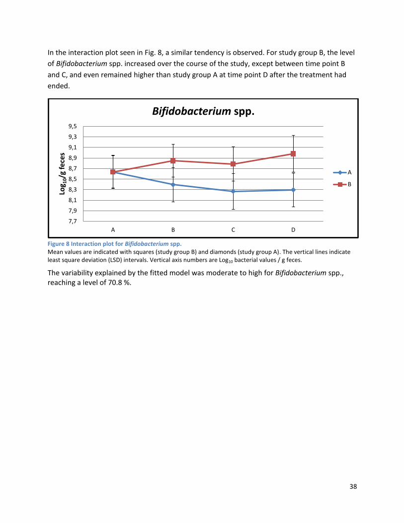
38
In the interaction plot seen in Fig. 8, a similar tendency is observed. For study group B, the level
of Bifidobacterium spp. increased over the course of the study, except between time point B
and C, and even remained higher than study group A at time point D after the treatment had
ended.
Figure 8 Interaction plot for Bifidobacterium spp. Mean values are indicated with squares (study group B) and diamonds (study group A). The vertical lines indicate least square deviation (LSD) intervals. Vertical axis numbers are Log10 bacterial values / g feces.
The variability explained by the fitted model was moderate to high for Bifidobacterium spp., reaching a level of 70.8 %.
7,7
7,9
8,1
8,3
8,5
8,7
8,9
9,1
9,3
9,5
A B C D
Log 1
0/g
fec
es
Bifidobacterium spp.
A
B
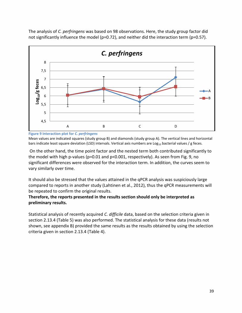
39
The analysis of C. perfringens was based on 98 observations. Here, the study group factor did not significantly influence the model (p=0.72), and neither did the interaction term (p=0.57).
Figure 9 Interaction plot for C. perfringens Mean values are indicated squares (study group B) and diamonds (study group A). The vertical lines and horizontal bars indicate least square deviation (LSD) intervals. Vertical axis numbers are Log10 bacterial values / g feces.
On the other hand, the time point factor and the nested term both contributed significantly to the model with high p-values (p=0.01 and p<0.001, respectively). As seen from Fig. 9, no significant differences were observed for the interaction term. In addition, the curves seem to vary similarly over time.
It should also be stressed that the values attained in the qPCR analysis was suspiciously large compared to reports in another study (Lahtinen et al., 2012), thus the qPCR measurements will be repeated to confirm the original results. Therefore, the reports presented in the results section should only be interpreted as preliminary results. Statistical analysis of recently acquired C. difficile data, based on the selection criteria given in section 2.13.4 (Table 5) was also performed. The statistical analysis for these data (results not shown, see appendix B) provided the same results as the results obtained by using the selection criteria given in section 2.13.4 (Table 4).
4,5
5
5,5
6
6,5
7
7,5
8
A B C D
Log 1
0/g
fec
es
C. perfringens
A
B
40
3.2 NMR
3.2.1 Pre-analysis phase
The NMR spectra acquired in the pre-analysis phase, on which decisions for further testing was based, are listed in appendix C. The spectra obtained from each individual testing experiment were assessed and evaluated before the pre-analysis phase was continued. The spectra were assessed primarily on basis of their spectral appearance, thus providing spectra of optimal quality. Here, the spectral appearance concept includes baseline uniformity, signal intensity and phase coherence, as well as the resolution of the spectrum. In the first tests, the addition of acid and alkaline in the preparation of samples was tested, as well as an initial comparison of pulse sequences, which was investigated further in the end of the pre-analysis phase. The addition of acid and alkaline induced baseline distortions to the spectra, especially the spectra with no acid added due to the higher pH of the prepared sample analysed. It should also be noted that the first test included a lipophilic sample extract (2.13.1.2, Results section). The initial pulse sequence comparison showed that the CPMG pulse sequence did provide a more uniform baseline compared to the ZGESGP sequence. In contrast, suppression of the water signal was significantly better in the ZGESGP sequence compared to the CPMG sequence. Although the ZGESGP sequence gave a better water suppression, the CPMG sequence was chosen to be utilized in subsequent tests due to the flatter baseline (2.13.1.4, Results section). Further on, the vortex mixing step was examined, as well as the effect of sonication and the number of extractions. The vortex mixing test clearly demonstrated that thorough vortex mixing was necessary to increase the intensity of the signals. Neither sonication nor extraction number did, however, provide any spectrum quality improvements or added any further information to the spectra, thus these steps were not implemented in the subsequent testing procedures (2.13.1.5 and 2.13.1.6, Results section). Afterwards, the sample weight-to-buffer volume ratio was tested with different combinations of sample weight and buffer volumes. The spectra from these tests showed that a more uniform baseline could be obtained with a lower ratio, but with diminished signal intensities. Thus a ratio between the lower and upper ratios showed an optimal level of baseline uniformity and signal intensity. The effect of filtration was also tested, but did not result in any significant improvements of the spectrum quality. In addition, an acid mixture was also spiked to the sample solution to test the degree of recovery of the acids after filtration. The acid mixture was based on acids detected in GC analysis. All except one acid was identified after filtration, thus the filtration step did not seem to affect the recovery rate of the acids (2.13.1.8 and 2.13.1.9, Results section). Subsequently, a biphasic extraction method was compared with methanol and PBS buffer extraction methods. The acid mixture mentioned above was also included in the biphasic extraction method to test the recovery of acids in the mixture after biphasic separation and
41
lyophilisation. The recovery rate of the acids was relatively high in the hydrophilic phase, but the expected intensity increase of the acid signals was not detectable. The acids could, however, not be recovered in the lipophilic extract. The method comparison (biphasic vs. Methanol vs. Buffer extraction) showed that methanol extraction provided relatively high intensity signals, but with low resolution. The hydrophilic phase of the biphasic extraction resulted in low intensity signals and poor resolution. The signals from the buffer extraction had lower intensity compared to the methanol extraction, but the resolution was better. Thus buffer extraction was preferred over the methanol extraction (2.13.1.10, Results section). This testing was followed by an optimization of the CPMG sequence, which resulted high resolution of the spectrum, and a relatively uniform, flat baseline. The optimized CPMG sequence was utilized in the subsequent tests (2.13.1.11, Results section). The CPMG optimization was followed by testing of the sample solubilisation. The test resulted in a spectrum where only few signals could be observed, and of relatively low intensity. This solubilisation method was, however, used in the subsequent tests (2.13.1.12, Results section). A range of tests of the effect on water suppression by the addition of NH4Cl to the sample solution was examined. From the resulting spectra, it was deduced that a concentration between 240 mM and 336 mM was sufficient to provide full water suppression (2.13.1.13, Results section). Subsequently, pulse sequences and sample dilutions were compared including the addition of NH4Cl to the sample solution. From the resulting spectra it could be seen that the combination of low dilution and CPMG sequence provided relatively high intensity signals with a decent resolution compared to applying the ZGESGP sequence to samples. The ZGESGP sequence did, however, provide better water suppression, as observed in previous tests. Furthermore, the addition of NH4Cl to the sample solution also resulted in water suppression, reaching the same efficiency as the ZGESGP sequence, but with slightly better resolution (2.13.1.14, Results section). Moreover, buffer with or without saline was also compared, and buffer without saline provided slightly more intense signals. Based on these results, a new test of pulse sequences and solvent was tested. From this test, similar results were obtained with buffer without saline providing slightly better resolution and intensity of signals compared to the buffer containing saline (2.13.1.15 and 2.13.1.16, Results section). Finally, a range of experiments were performed, in which combinations of pulse sequences, sample dilution and preparation procedure was tested. The spectra obtained showed that the CPMG sequence provided higher signal intensities compared to the NOESY and ZGESP, whereas the latter sequences resulted in better water suppression. Furthermore, additional intensity gains were achieved for less diluted samples. Although the spectra comparison seemed to favour inclusion of sonication and freeze-thawing cycles to the preparation procedure due to more intense signals, baseline distortions and lower resolution was observed when including these steps in the preparation procedure. Thus a faster preparation procedure was opted for in the analysis phase, leading to a more uniform baseline and higher resolution of compounds, albeit at the expense of intensity (2.13.1.17, Results section).
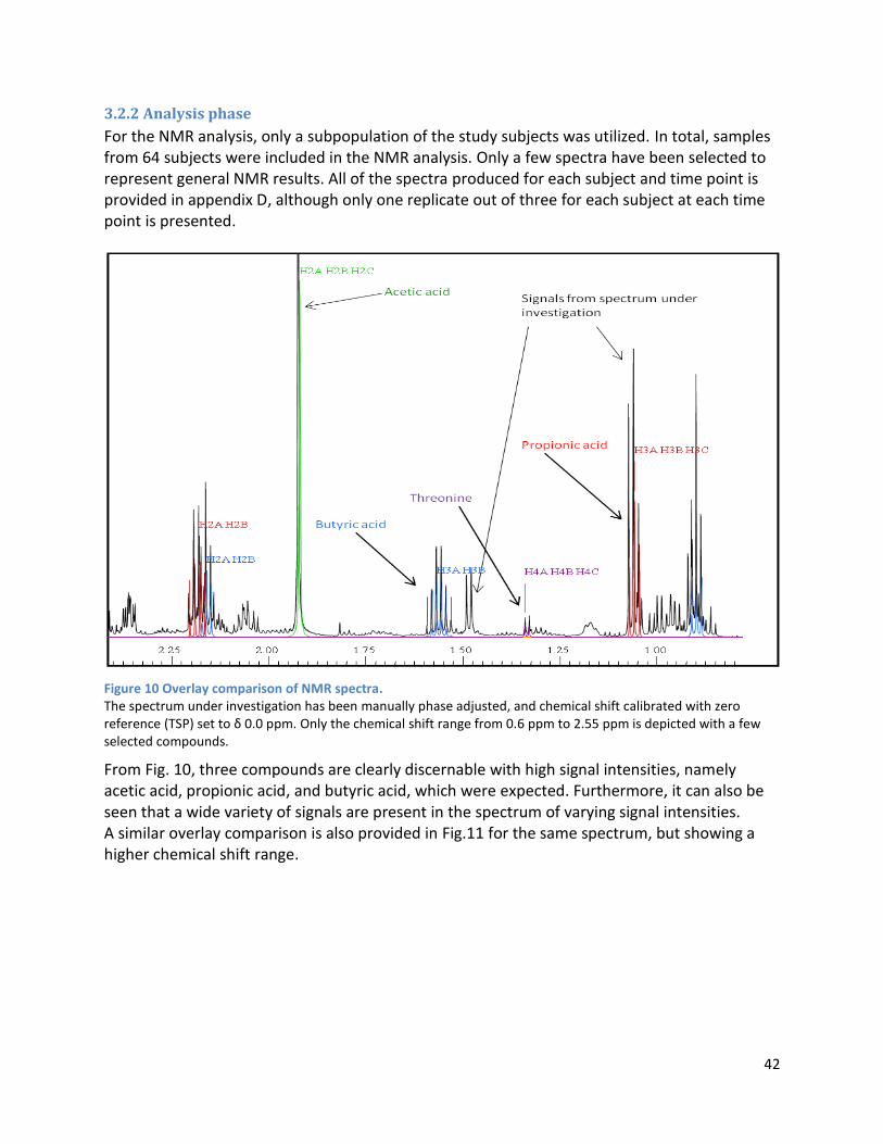
42
3.2.2 Analysis phase
For the NMR analysis, only a subpopulation of the study subjects was utilized. In total, samples from 64 subjects were included in the NMR analysis. Only a few spectra have been selected to represent general NMR results. All of the spectra produced for each subject and time point is provided in appendix D, although only one replicate out of three for each subject at each time point is presented.
Figure 10 Overlay comparison of NMR spectra. The spectrum under investigation has been manually phase adjusted, and chemical shift calibrated with zero reference (TSP) set to δ 0.0 ppm. Only the chemical shift range from 0.6 ppm to 2.55 ppm is depicted with a few selected compounds.
From Fig. 10, three compounds are clearly discernable with high signal intensities, namely acetic acid, propionic acid, and butyric acid, which were expected. Furthermore, it can also be seen that a wide variety of signals are present in the spectrum of varying signal intensities. A similar overlay comparison is also provided in Fig.11 for the same spectrum, but showing a higher chemical shift range.
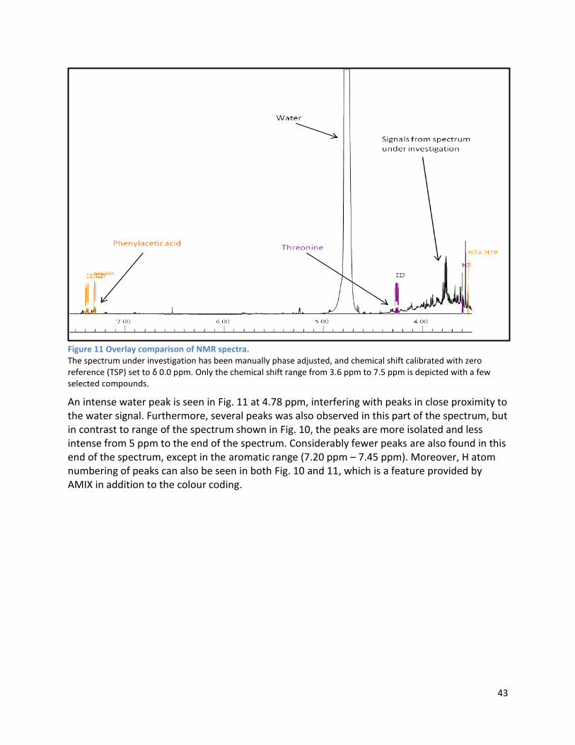
43
Figure 11 Overlay comparison of NMR spectra. The spectrum under investigation has been manually phase adjusted, and chemical shift calibrated with zero reference (TSP) set to δ 0.0 ppm. Only the chemical shift range from 3.6 ppm to 7.5 ppm is depicted with a few selected compounds.
An intense water peak is seen in Fig. 11 at 4.78 ppm, interfering with peaks in close proximity to the water signal. Furthermore, several peaks was also observed in this part of the spectrum, but in contrast to range of the spectrum shown in Fig. 10, the peaks are more isolated and less intense from 5 ppm to the end of the spectrum. Considerably fewer peaks are also found in this end of the spectrum, except in the aromatic range (7.20 ppm – 7.45 ppm). Moreover, H atom numbering of peaks can also be seen in both Fig. 10 and 11, which is a feature provided by AMIX in addition to the colour coding.
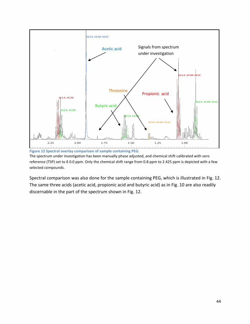
44
Figure 12 Spectral overlay comparison of sample containing PEG. The spectrum under investigation has been manually phase adjusted, and chemical shift calibrated with zero
reference (TSP) set to δ 0.0 ppm. Only the chemical shift range from 0.8 ppm to 2.425 ppm is depicted with a few
selected compounds.
Spectral comparison was also done for the sample containing PEG, which is illustrated in Fig. 12.
The same three acids (acetic acid, propionic acid and butyric acid) as in Fig. 10 are also readily
discernable in the part of the spectrum shown in Fig. 12.
2.25 2.00 1.75 1.50 1.25 1.00
H2A H2B H2C
H2A H2B
H3A H3B
H4A H4B H4C
H2A H2B
H3A H3B H3C
H4A H4B H4C
Butyric acid
Acetic acid
Propionic acid Threonine
Signals from spectrum
under investigation
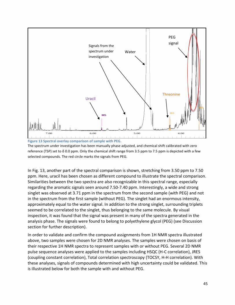
45
Figure 13 Spectral overlay comparison of sample with PEG. The spectrum under investigation has been manually phase adjusted, and chemical shift calibrated with zero
reference (TSP) set to δ 0.0 ppm. Only the chemical shift range from 3.5 ppm to 7.5 ppm is depicted with a few
selected compounds. The red circle marks the signals from PEG.
In Fig. 13, another part of the spectral comparison is shown, stretching from 3.50 ppm to 7.50 ppm. Here, uracil has been chosen as different compound to illustrate the spectral comparison. Similarities between the two spectra are also recognizable in this spectral range, especially regarding the aromatic signals seen around 7.50-7.40 ppm. Interestingly, a wide and strong singlet was observed at 3.71 ppm in the spectrum from the second sample (with PEG) and not in the spectrum from the first sample (without PEG). The singlet had an enormous intensity, approximately equal to the water signal. In addition to the strong singlet, surrounding triplets seemed to be correlated to the singlet, thus belonging to the same molecule. By visual inspection, it was found that the signal was present in many of the spectra generated in the analysis phase. The signals were found to belong to polyethylene glycol (PEG) (see Discussion section for further description).
In order to validate and confirm the compound assignments from 1H NMR spectra illustrated above, two samples were chosen for 2D NMR analyses. The samples were chosen on basis of their respective 1H NMR spectra to represent samples with or without PEG. Several 2D NMR pulse sequence analyses were applied to the samples including HSQC (H-C correlation), JRES (coupling constant correlation), Total correlation spectroscopy (TOCSY, H-H correlation). With these analyses, signals of compounds determined with high uncertainty could be validated. This is illustrated below for both the sample with and without PEG.
7.00 6.00 5.00 4.00
H3
H2
H5H5
Threonine Uracil
Water
Signals from the
spectrum under
investigation
PEG
signal
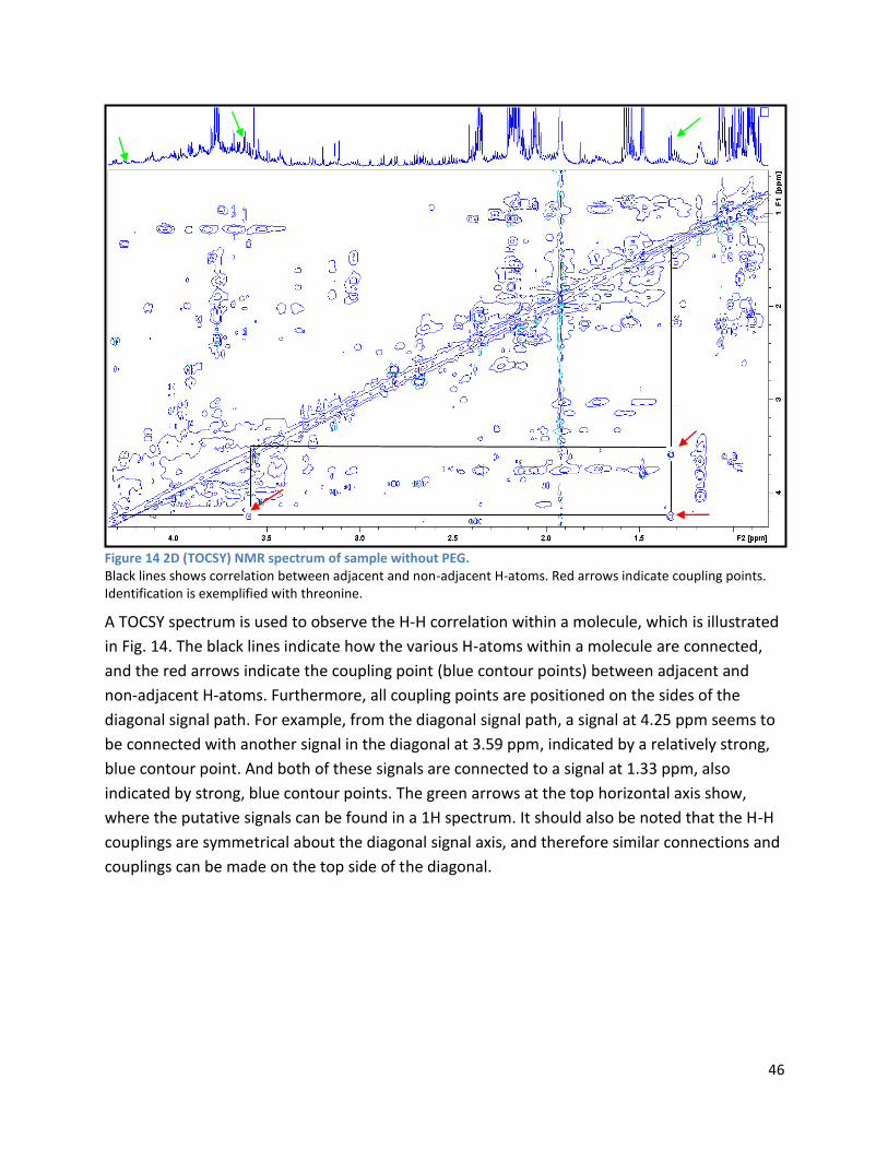
46
Figure 14 2D (TOCSY) NMR spectrum of sample without PEG. Black lines shows correlation between adjacent and non-adjacent H-atoms. Red arrows indicate coupling points. Identification is exemplified with threonine.
A TOCSY spectrum is used to observe the H-H correlation within a molecule, which is illustrated
in Fig. 14. The black lines indicate how the various H-atoms within a molecule are connected,
and the red arrows indicate the coupling point (blue contour points) between adjacent and
non-adjacent H-atoms. Furthermore, all coupling points are positioned on the sides of the
diagonal signal path. For example, from the diagonal signal path, a signal at 4.25 ppm seems to
be connected with another signal in the diagonal at 3.59 ppm, indicated by a relatively strong,
blue contour point. And both of these signals are connected to a signal at 1.33 ppm, also
indicated by strong, blue contour points. The green arrows at the top horizontal axis show,
where the putative signals can be found in a 1H spectrum. It should also be noted that the H-H
couplings are symmetrical about the diagonal signal axis, and therefore similar connections and
couplings can be made on the top side of the diagonal.
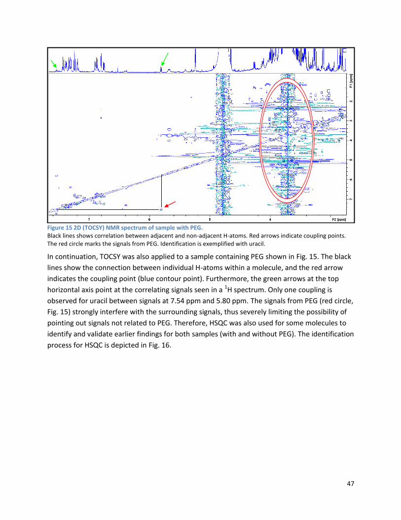
47
Figure 15 2D (TOCSY) NMR spectrum of sample with PEG. Black lines shows correlation between adjacent and non-adjacent H-atoms. Red arrows indicate coupling points. The red circle marks the signals from PEG. Identification is exemplified with uracil.
In continuation, TOCSY was also applied to a sample containing PEG shown in Fig. 15. The black
lines show the connection between individual H-atoms within a molecule, and the red arrow
indicates the coupling point (blue contour point). Furthermore, the green arrows at the top
horizontal axis point at the correlating signals seen in a 1H spectrum. Only one coupling is
observed for uracil between signals at 7.54 ppm and 5.80 ppm. The signals from PEG (red circle,
Fig. 15) strongly interfere with the surrounding signals, thus severely limiting the possibility of
pointing out signals not related to PEG. Therefore, HSQC was also used for some molecules to
identify and validate earlier findings for both samples (with and without PEG). The identification
process for HSQC is depicted in Fig. 16.
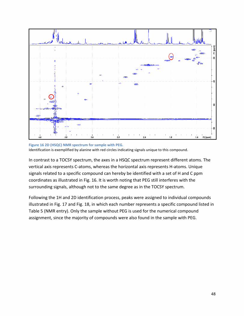
48
Figure 16 2D (HSQC) NMR spectrum for sample with PEG. Identification is exemplified by alanine with red circles indicating signals unique to this compound.
In contrast to a TOCSY spectrum, the axes in a HSQC spectrum represent different atoms. The
vertical axis represents C-atoms, whereas the horizontal axis represents H-atoms. Unique
signals related to a specific compound can hereby be identified with a set of H and C ppm
coordinates as illustrated in Fig. 16. It is worth noting that PEG still interferes with the
surrounding signals, although not to the same degree as in the TOCSY spectrum.
Following the 1H and 2D identification process, peaks were assigned to individual compounds
illustrated in Fig. 17 and Fig. 18, in which each number represents a specific compound listed in
Table 5 (NMR entry). Only the sample without PEG is used for the numerical compound
assignment, since the majority of compounds were also found in the sample with PEG.

49
Figure 17 NMR spectrum with compound assignments Identical numbers indicate peaks belonging to the same compound. Underlined numbers indicate compounds, where not all peaks were identified by 1H NMR.
In the part of the spectrum shown in Fig. 17 (0.0 ppm – 4.30 ppm), short chain fatty acids
(SCFAs) comprised of acetic acid, propionic acid and butyric acid were identified. Additionally,
isovaleric acid and isobutyric acid were also identified. All of the SCFAs showed relatively high
signal intensities, especially acetic acid. The BCFAs showed moderate signal intensities with
isovaleric acid having a higher intensity compared to isobutyric acid. Moreover, organic acids
including pyruvic acid, succinic acid, malic acid and fumaric acid were also identified. All organic
acids exhibited low signal intensities, except succinic acid and fumaric acid demonstrating
relatively high and moderate signal intensities, respectively. Furthermore, both ionisable amino
acids, such as lysine and glutamic acid, as well as hydrophilic and hydrophobic amino acids
including threonine and leucine were identified in this part of the spectrum. Unexpectedly,
lactic acid was not identified in the samples, neither in 1H or 2D NMR. Moreover, the presence
of amine compounds, such as trimethylamine and its oxide derivative (trimethyl-N-oxide) was
also detected, although showing relatively low intensities.
23
24
25
29
30
31
32
33
34
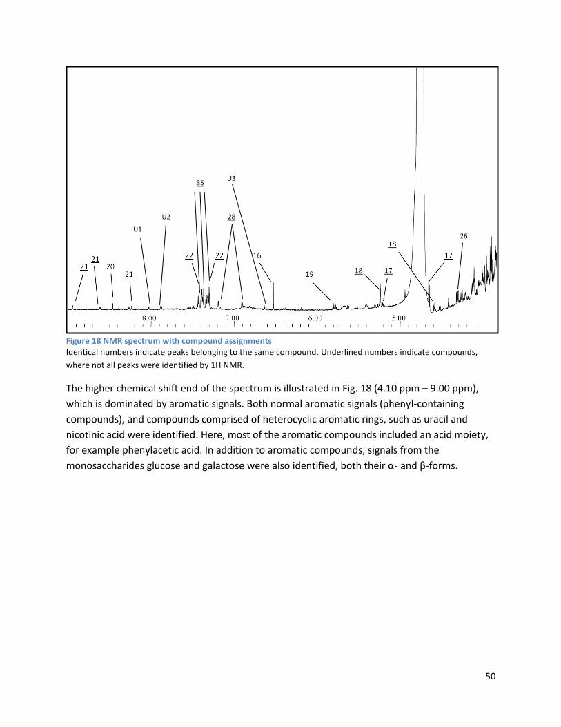
50
Figure 18 NMR spectrum with compound assignments Identical numbers indicate peaks belonging to the same compound. Underlined numbers indicate compounds,
where not all peaks were identified by 1H NMR.
The higher chemical shift end of the spectrum is illustrated in Fig. 18 (4.10 ppm – 9.00 ppm),
which is dominated by aromatic signals. Both normal aromatic signals (phenyl-containing
compounds), and compounds comprised of heterocyclic aromatic rings, such as uracil and
nicotinic acid were identified. Here, most of the aromatic compounds included an acid moiety,
for example phenylacetic acid. In addition to aromatic compounds, signals from the
monosaccharides glucose and galactose were also identified, both their α- and β-forms.
26
28
U1
U2
U3 35
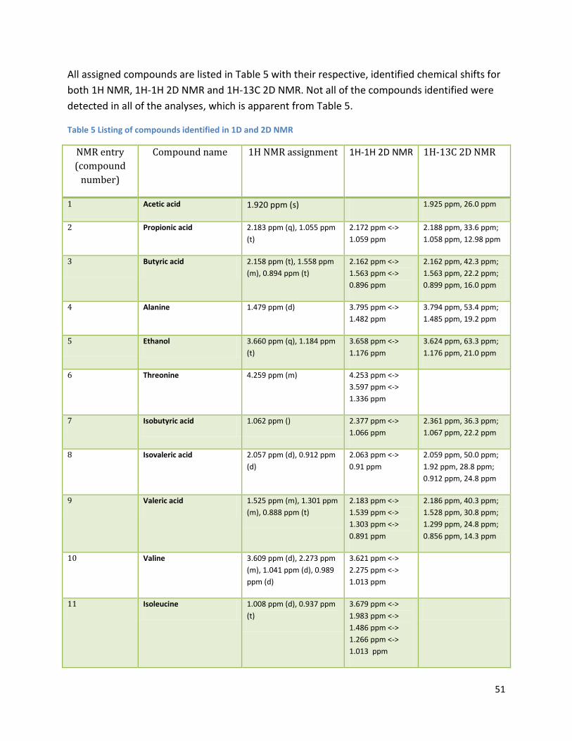
51
All assigned compounds are listed in Table 5 with their respective, identified chemical shifts for
both 1H NMR, 1H-1H 2D NMR and 1H-13C 2D NMR. Not all of the compounds identified were
detected in all of the analyses, which is apparent from Table 5.
Table 5 Listing of compounds identified in 1D and 2D NMR
NMR entry
(compound
number)
Compound name 1H NMR assignment 1H-1H 2D NMR 1H-13C 2D NMR
1 Acetic acid 1.920 ppm (s) 1.925 ppm, 26.0 ppm
2 Propionic acid 2.183 ppm (q), 1.055 ppm
(t)
2.172 ppm <->
1.059 ppm
2.188 ppm, 33.6 ppm;
1.058 ppm, 12.98 ppm
3 Butyric acid 2.158 ppm (t), 1.558 ppm
(m), 0.894 ppm (t)
2.162 ppm <->
1.563 ppm <->
0.896 ppm
2.162 ppm, 42.3 ppm;
1.563 ppm, 22.2 ppm;
0.899 ppm, 16.0 ppm
4 Alanine 1.479 ppm (d) 3.795 ppm <->
1.482 ppm
3.794 ppm, 53.4 ppm;
1.485 ppm, 19.2 ppm
5 Ethanol 3.660 ppm (q), 1.184 ppm
(t)
3.658 ppm <->
1.176 ppm
3.624 ppm, 63.3 ppm;
1.176 ppm, 21.0 ppm
6 Threonine 4.259 ppm (m) 4.253 ppm <->
3.597 ppm <->
1.336 ppm
7 Isobutyric acid 1.062 ppm () 2.377 ppm <->
1.066 ppm
2.361 ppm, 36.3 ppm;
1.067 ppm, 22.2 ppm
8 Isovaleric acid 2.057 ppm (d), 0.912 ppm
(d)
2.063 ppm <->
0.91 ppm
2.059 ppm, 50.0 ppm;
1.92 ppm, 28.8 ppm;
0.912 ppm, 24.8 ppm
9 Valeric acid 1.525 ppm (m), 1.301 ppm
(m), 0.888 ppm (t)
2.183 ppm <->
1.539 ppm <->
1.303 ppm <->
0.891 ppm
2.186 ppm, 40.3 ppm;
1.528 ppm, 30.8 ppm;
1.299 ppm, 24.8 ppm;
0.856 ppm, 14.3 ppm
10 Valine 3.609 ppm (d), 2.273 ppm
(m), 1.041 ppm (d), 0.989
ppm (d)
3.621 ppm <->
2.275 ppm <->
1.013 ppm
11 Isoleucine 1.008 ppm (d), 0.937 ppm
(t)
3.679 ppm <->
1.983 ppm <->
1.486 ppm <->
1.266 ppm <->
1.013 ppm
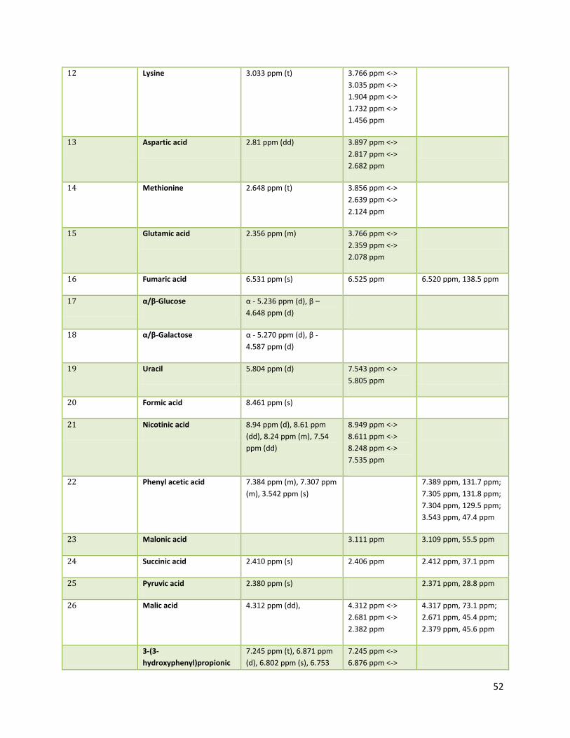
52
12 Lysine 3.033 ppm (t) 3.766 ppm <->
3.035 ppm <->
1.904 ppm <->
1.732 ppm <->
1.456 ppm
13 Aspartic acid 2.81 ppm (dd) 3.897 ppm <->
2.817 ppm <->
2.682 ppm
14 Methionine 2.648 ppm (t) 3.856 ppm <->
2.639 ppm <->
2.124 ppm
15 Glutamic acid 2.356 ppm (m) 3.766 ppm <->
2.359 ppm <->
2.078 ppm
16 Fumaric acid 6.531 ppm (s) 6.525 ppm 6.520 ppm, 138.5 ppm
17 α/β-Glucose α - 5.236 ppm (d), β –
4.648 ppm (d)
18 α/β-Galactose α - 5.270 ppm (d), β -
4.587 ppm (d)
19 Uracil 5.804 ppm (d) 7.543 ppm <->
5.805 ppm
20 Formic acid 8.461 ppm (s)
21 Nicotinic acid 8.94 ppm (d), 8.61 ppm
(dd), 8.24 ppm (m), 7.54
ppm (dd)
8.949 ppm <->
8.611 ppm <->
8.248 ppm <->
7.535 ppm
22 Phenyl acetic acid 7.384 ppm (m), 7.307 ppm
(m), 3.542 ppm (s)
7.389 ppm, 131.7 ppm;
7.305 ppm, 131.8 ppm;
7.304 ppm, 129.5 ppm;
3.543 ppm, 47.4 ppm
23 Malonic acid 3.111 ppm 3.109 ppm, 55.5 ppm
24 Succinic acid 2.410 ppm (s) 2.406 ppm 2.412 ppm, 37.1 ppm
25 Pyruvic acid 2.380 ppm (s) 2.371 ppm, 28.8 ppm
26 Malic acid 4.312 ppm (dd), 4.312 ppm <->
2.681 ppm <->
2.382 ppm
4.317 ppm, 73.1 ppm;
2.671 ppm, 45.4 ppm;
2.379 ppm, 45.6 ppm
3-(3-
hydroxyphenyl)propionic
7.245 ppm (t), 6.871 ppm
(d), 6.802 ppm (s), 6.753
7.245 ppm <->
6.876 ppm <->
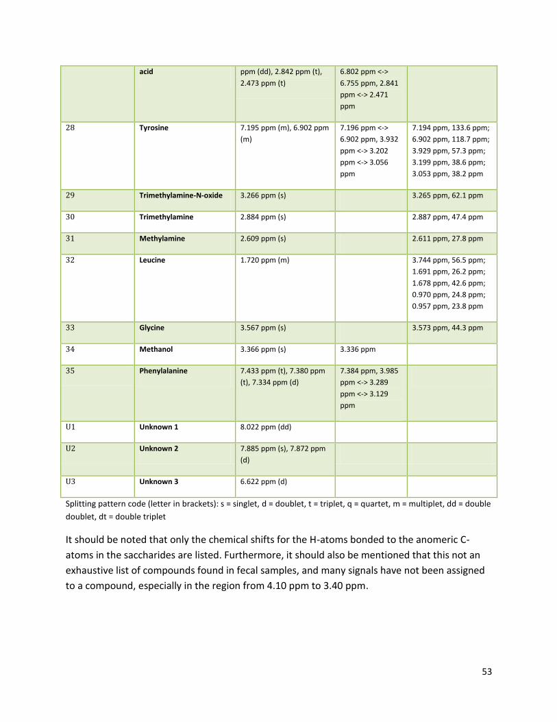
53
acid ppm (dd), 2.842 ppm (t),
2.473 ppm (t)
6.802 ppm <->
6.755 ppm, 2.841
ppm <-> 2.471
ppm
28 Tyrosine 7.195 ppm (m), 6.902 ppm
(m)
7.196 ppm <->
6.902 ppm, 3.932
ppm <-> 3.202
ppm <-> 3.056
ppm
7.194 ppm, 133.6 ppm;
6.902 ppm, 118.7 ppm;
3.929 ppm, 57.3 ppm;
3.199 ppm, 38.6 ppm;
3.053 ppm, 38.2 ppm
29 Trimethylamine-N-oxide 3.266 ppm (s) 3.265 ppm, 62.1 ppm
30 Trimethylamine 2.884 ppm (s) 2.887 ppm, 47.4 ppm
31 Methylamine 2.609 ppm (s) 2.611 ppm, 27.8 ppm
32 Leucine 1.720 ppm (m) 3.744 ppm, 56.5 ppm;
1.691 ppm, 26.2 ppm;
1.678 ppm, 42.6 ppm;
0.970 ppm, 24.8 ppm;
0.957 ppm, 23.8 ppm
33 Glycine 3.567 ppm (s) 3.573 ppm, 44.3 ppm
34 Methanol 3.366 ppm (s) 3.336 ppm
35 Phenylalanine 7.433 ppm (t), 7.380 ppm
(t), 7.334 ppm (d)
7.384 ppm, 3.985
ppm <-> 3.289
ppm <-> 3.129
ppm
U1 Unknown 1 8.022 ppm (dd)
U2 Unknown 2 7.885 ppm (s), 7.872 ppm
(d)
U3 Unknown 3 6.622 ppm (d)
Splitting pattern code (letter in brackets): s = singlet, d = doublet, t = triplet, q = quartet, m = multiplet, dd = double
doublet, dt = double triplet
It should be noted that only the chemical shifts for the H-atoms bonded to the anomeric C-
atoms in the saccharides are listed. Furthermore, it should also be mentioned that this not an
exhaustive list of compounds found in fecal samples, and many signals have not been assigned
to a compound, especially in the region from 4.10 ppm to 3.40 ppm.
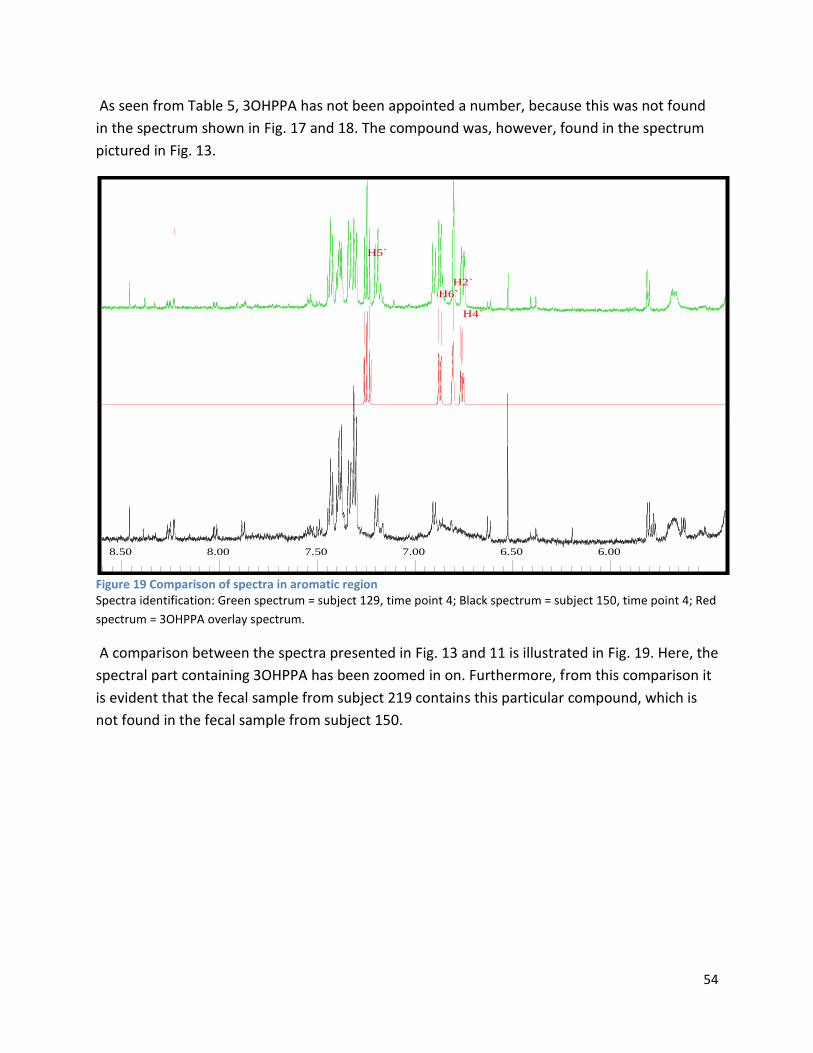
54
As seen from Table 5, 3OHPPA has not been appointed a number, because this was not found
in the spectrum shown in Fig. 17 and 18. The compound was, however, found in the spectrum
pictured in Fig. 13.
Figure 19 Comparison of spectra in aromatic region Spectra identification: Green spectrum = subject 129, time point 4; Black spectrum = subject 150, time point 4; Red
spectrum = 3OHPPA overlay spectrum.
A comparison between the spectra presented in Fig. 13 and 11 is illustrated in Fig. 19. Here, the
spectral part containing 3OHPPA has been zoomed in on. Furthermore, from this comparison it
is evident that the fecal sample from subject 219 contains this particular compound, which is
not found in the fecal sample from subject 150.
8.50 8.00 7.50 7.00 6.50 6.00
H5`
H6`
H2`
H4`
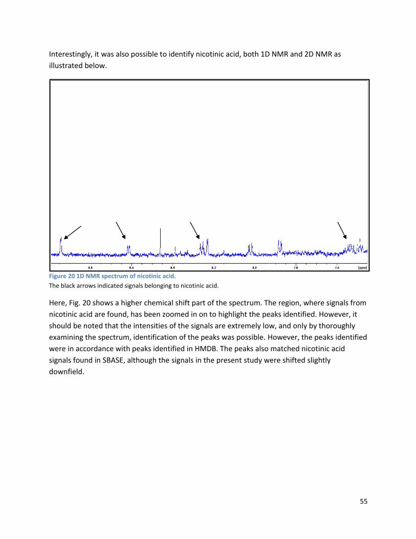
55
Interestingly, it was also possible to identify nicotinic acid, both 1D NMR and 2D NMR as
illustrated below.
Figure 20 1D NMR spectrum of nicotinic acid.
The black arrows indicated signals belonging to nicotinic acid.
Here, Fig. 20 shows a higher chemical shift part of the spectrum. The region, where signals from
nicotinic acid are found, has been zoomed in on to highlight the peaks identified. However, it
should be noted that the intensities of the signals are extremely low, and only by thoroughly
examining the spectrum, identification of the peaks was possible. However, the peaks identified
were in accordance with peaks identified in HMDB. The peaks also matched nicotinic acid
signals found in SBASE, although the signals in the present study were shifted slightly
downfield.
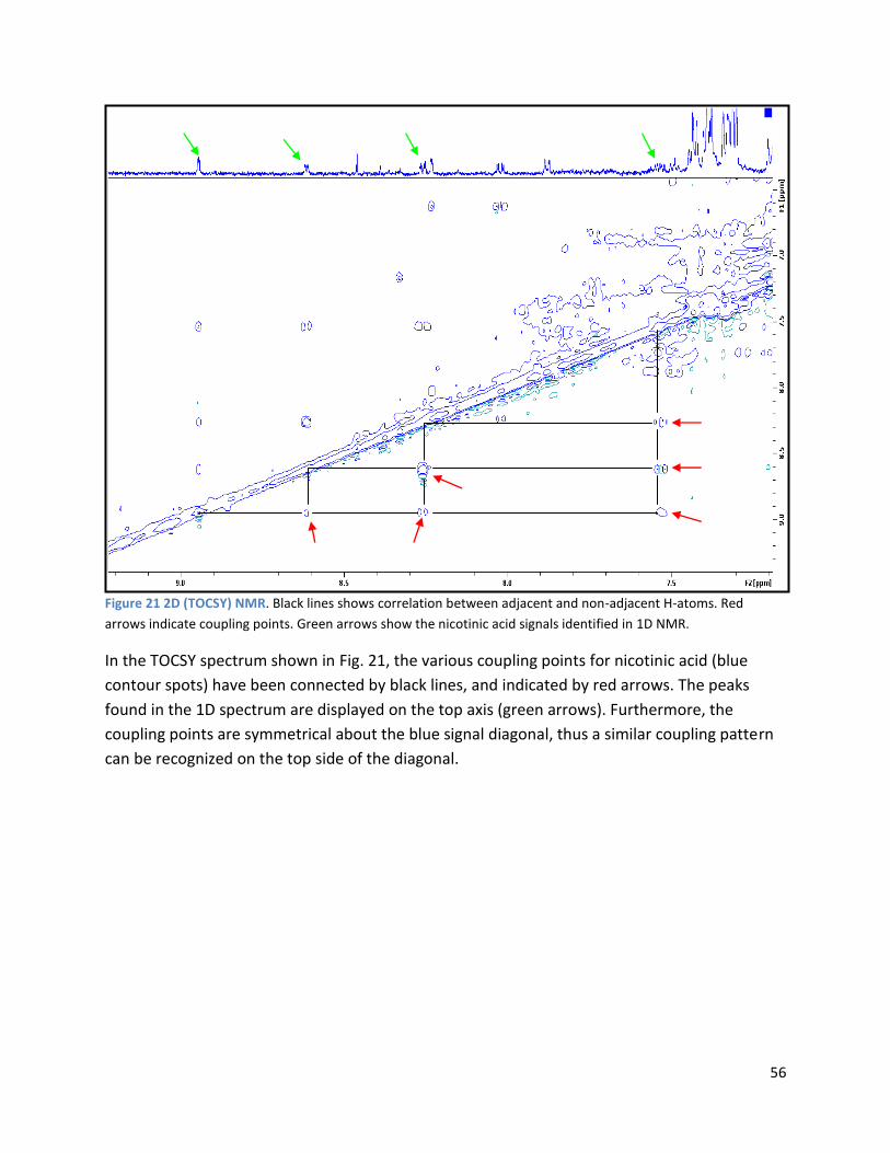
56
Figure 21 2D (TOCSY) NMR. Black lines shows correlation between adjacent and non-adjacent H-atoms. Red
arrows indicate coupling points. Green arrows show the nicotinic acid signals identified in 1D NMR.
In the TOCSY spectrum shown in Fig. 21, the various coupling points for nicotinic acid (blue
contour spots) have been connected by black lines, and indicated by red arrows. The peaks
found in the 1D spectrum are displayed on the top axis (green arrows). Furthermore, the
coupling points are symmetrical about the blue signal diagonal, thus a similar coupling pattern
can be recognized on the top side of the diagonal.
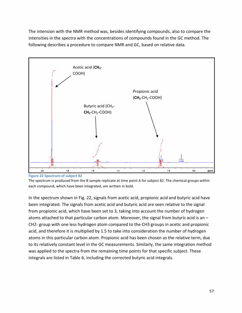
57
The intension with the NMR method was, besides identifying compounds, also to compare the
intensities in the spectra with the concentrations of compounds found in the GC method. The
following describes a procedure to compare NMR and GC, based on relative data.
Figure 22 Spectrum of subject 82 The spectrum is produced from the B sample replicate at time point A for subject 82. The chemical groups within
each compound, which have been integrated, are written in bold.
In the spectrum shown in Fig. 22, signals from acetic acid, propionic acid and butyric acid have
been integrated. The signals from acetic acid and butyric acid are seen relative to the signal
from propionic acid, which have been set to 3, taking into account the number of hydrogen
atoms attached to that particular carbon atom. Moreover, the signal from butyric acid is an –
CH2- group with one less hydrogen atom compared to the CH3 groups in acetic and propionic
acid, and therefore it is multiplied by 1.5 to take into consideration the number of hydrogen
atoms in this particular carbon atom. Propionic acid has been chosen as the relative term, due
to its relatively constant level in the GC measurements. Similarly, the same integration method
was applied to the spectra from the remaining time points for that specific subject. These
integrals are listed in Table 6, including the corrected butyric acid integrals.
Acetic acid (CH3-
COOH)
Butyric acid (CH3-
CH2-CH2-COOH)
Propionic acid
(CH3-CH2-COOH)
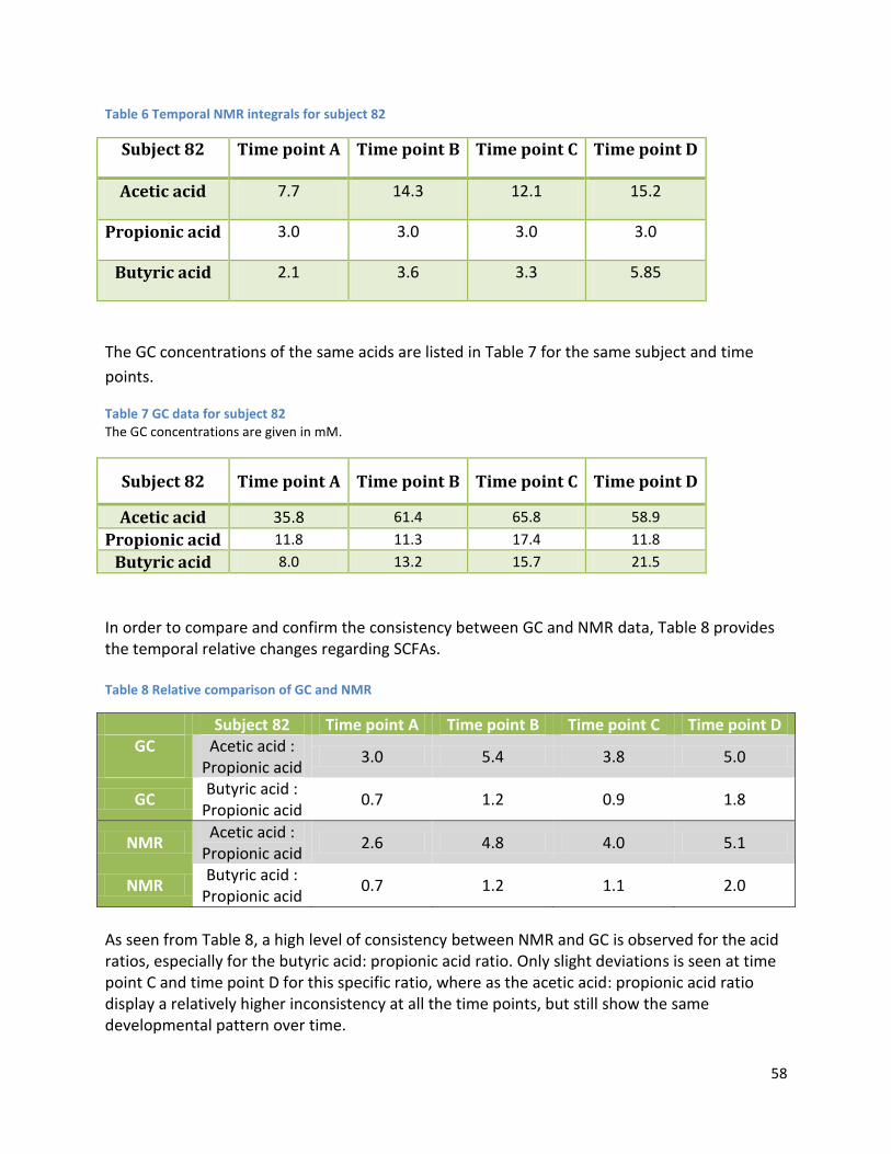
58
Table 6 Temporal NMR integrals for subject 82
Subject 82 Time point A Time point B Time point C Time point D
Acetic acid 7.7 14.3 12.1 15.2
Propionic acid 3.0 3.0 3.0 3.0
Butyric acid 2.1 3.6 3.3 5.85
The GC concentrations of the same acids are listed in Table 7 for the same subject and time
points.
Table 7 GC data for subject 82 The GC concentrations are given in mM.
Subject 82 Time point A Time point B Time point C Time point D
Acetic acid 35.8 61.4 65.8 58.9
Propionic acid 11.8 11.3 17.4 11.8
Butyric acid 8.0 13.2 15.7 21.5
In order to compare and confirm the consistency between GC and NMR data, Table 8 provides the temporal relative changes regarding SCFAs. Table 8 Relative comparison of GC and NMR
Subject 82 Time point A Time point B Time point C Time point D GC
Acetic acid :
Propionic acid 3.0 5.4 3.8 5.0
GC Butyric acid :
Propionic acid 0.7 1.2 0.9 1.8
NMR Acetic acid :
Propionic acid 2.6 4.8 4.0 5.1
NMR Butyric acid :
Propionic acid 0.7 1.2 1.1 2.0
As seen from Table 8, a high level of consistency between NMR and GC is observed for the acid ratios, especially for the butyric acid: propionic acid ratio. Only slight deviations is seen at time point C and time point D for this specific ratio, where as the acetic acid: propionic acid ratio display a relatively higher inconsistency at all the time points, but still show the same developmental pattern over time.
59
Based on visual inspection of the spectra used in the comparison above, the same level of consistency between the GC data and the NMR spectra intensities was observed for isovaleric acid and valeric acid (not shown). A general concern working with biological samples is reproducibility, especially the preparation of samples. A comparison between replicate of samples is given in appendix E. These comparisons show that some of the samples do demonstrate a relatively high degree of variability regarding peak intensities; especially for subject 11 at time point C. An interesting observation is a wide bump in close proximity of the water signal in this comparison. However, this particular bump is also observed in the other comparisons, but to a markedly lesser degree. Although differences in signal intensities are observed, no apparent spectral signal differences are seen.
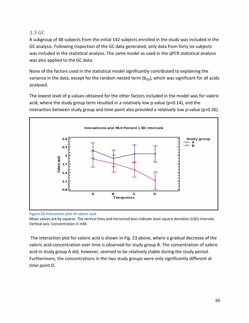
60
3.3 GC
A subgroup of 48 subjects from the initial 142 subjects enrolled in the study was included in the
GC analysis. Following inspection of the GC data generated, only data from forty six subjects
was included in the statistical analysis. The same model as used in the qPCR statistical analysis
was also applied to the GC data.
None of the factors used in the statistical model significantly contributed to explaining the
variance in the data, except for the random nested term (bi(j)), which was significant for all acids
analysed.
The lowest level of p-values obtained for the other factors included in the model was for valeric
acid, where the study group term resulted in a relatively low p-value (p=0.14), and the
interaction between study group and time point also provided a relatively low p-value (p=0.26).
Figure 23 Interaction plot of valeric acid Mean values are by squares. The vertical lines and horizontal bars indicate least square deviation (LSD) intervals. Vertical axis: Concentration in mM.
The interaction plot for valeric acid is shown in Fig. 23 above, where a gradual decrease of the
valeric acid concentration over time is observed for study group B. The concentration of valeric
acid in study group A did, however, seemed to be relatively stable during the study period.
Furthermore, the concentrations in the two study groups were only significantly different at
time point D.
Interactions and 95.0 Percent LSD Intervals
Timepoints
0.8
1.1
1.4
1.7
2
2.3
2.6
Val
eric
aci
d
A B C D
Study_groupAB

61
As seen from Fig. 24, study group A tended to have a higher concentration of valeric acid
compared to study group B, in accordance with the relatively low p-value for this factor.
Figure 24 Means plot of study group for valeric acid Mean values are indicated with open circles. The vertical lines and horizontal bars indicate least square deviation (LSD) intervals. Vertical axis: Concentration in mM. The time points have been pooled together for each individual and for each study group.
All interaction plots and means plots, as well as sum of squares and analysis of variance tables
for each acid can be found in appendix F. Furthermore, all GC data used in the statistical
analysis is provided in appendix G.
A B
Means and 95.0 Percent LSD Interv als
Study_group
1.2
1.4
1.6
1.8
2
2.2
2.4
Val
eric
aci
d
62
4 Discussion
4.1 qPCR
The current study explored the effect of the probiotic L. acidophilus NCFM consumption on the
level of C. difficile in elderly people. In this study, no significant difference was observed
between the study groups, thus the ingestion of L. acidophilus NCFM did not seem to affect the
level of C. difficile. To this author´s knowledge, no present study has been conducted set up in a
parallel manner as the current study including the same probiotic strain and the same age
group. However, in a comparable study performed by Lahtinen et al. (2012), healthy elderly
subjects consumed cheese containing L. acidophilus NCFM and L. rhamnosus HN001. In this
study, a reduction in the level of C. difficile was observed for the probiotic group, which is
contradictory to the findings in the current study. This could possibly be explained by the
inclusion of two probiotic strains in the cheese consumed, causing a synergy between the two
study probiotic strains. In addition, the current study and the study executed by Lahtinen et al.
(2012) also differed on the design of the studies. In the case of Lahtinen et al. (2012), the study
was designed as a cross-over study, in which every subject acts as its own control, thus
minimizing the inter-individual variation, which is very common in human studies. This was not
the case in the present study, where subjects were divided into a control group and a
treatment group.
Furthermore, it was also noted in Lahtinen et al. (2012) that the initial level of C. difficile was
relatively low for the whole study group, which was not the case in the current study. In fact, a
high initial variation in the level of C. difficile was seen for the entire study group, which, in part,
could explain why no group differences were observed. Moreover, the task of identifying C.
difficile in the faecal samples proved to be difficult, because this bacterium is often found in
very low numbers in the colon close to the detection limit for qPCR analysis. This is one of the
reasons, why C. difficile was below detection level in several subjects. Moreover, many of the C.
difficile results were only determined by one replicate, which introduces considerable variation
into the statistical analysis.
On the other hand, ingestion of L. acidophilus NCFM affected the level of Bifidobacterium spp.,
where consumption of the probiotic led to increases in these species, supporting observations
made in a recent study by Björklund et al. (2012), where the study group consumed a synbiotic
(combination of L. acidophilus NCFM and lactitol). The elderly subjects from that study were
prescribed a specific type of anti-inflammatory drugs, leading to certain study differences
between the current study and that of Björklund et al. (2012).
Although the studies differ, a plausible explanation for the same development observed for
Bifidobacterium ssp. is that the probiotic and synbiotics created an advantageous
microenvironment for the Bifidobacterium spp. by applying one or more of the probiotic modes
of action (microbial exclusion, nutrient competition etc.), causing a rise in bifidobacteria.
63
In accordance with the current study, other studies investigating the effect of probiotics on the
colonic microbiota found changes in the level of specific species from the intestinal microbiota,
although to varying degrees (Larsen et al., 2006; Mättö et al., 2006; Wang et al., 2012). Possible
factors explaining the different results include study design, length of study, number of study
participants, as well as differences in level of probiotic doses utilized and the probiotic strains
used. Especially the probiotic strains used greatly influence the outcome of the studies, since
effects of probiotics are generally restricted to a specific strain, and cannot be extrapolated to
other strains. Furthermore, the findings in Wang et al. (2012) could indicate that the effects of
probiotics are limited to short-term interventions, which is in agreement with Larsen et al.
(2006) and the present study.
Interestingly, the studies mentioned above all examined the effect of probiotic cocktails
containing more than one probiotic strain, or a synbiotic comprised of a probiotic strain and a
prebiotic oligosaccharide. Thus the reason for obtaining a different result in the current study
could possibly be related to the absent inter-bacterial synergy existing in these studies.
4.2 NMR
This study also resulted in the development of an NMR preparation procedure for faecal samples, as well as NMR analysis of a subset of the study population.
4.2.1 Pre-Analysis phase
In one of the first tests, addition of NaOH and formic acid to faecal samples was included in the procedure. According to Jacobs et al. (2008), the addition of alkaline should prevent loss of volatile compounds during lyophilisation, presumably by shifting the equilibrium of the acids in the sample toward its protonated form. And the addition of formic acid should stabilise phenolic compounds, which were examined in that particular study. The addition of acid and alkaline did, however, not seem to prevent the loss of volatile components. The addition of alkaline was also tested in later experiments, and no prevention of compound loss was observed in these experiments either. This is likely due to the dramatic changes in pH, which was observed to increase to pH≈12, although a low concentration of alkaline was used. For these experiments, no pulse sequence had been optimized, which would also contribute to the outcome of these particular experiments. Only low intensities of phenolic compounds were observed, even when acid was added to the sample. Therefore, these steps to the procedure were abandoned. The inclusion of sonication to the procedure was also tested to examine, if this additional step would provide better solubilisation of the faecal sample. Here, the improved solubilisation would be both due to cell membrane disruption caused by sonication with a concomitant release of intra-cellular material, but also breaking of possible micelles formed in the preparation process. In addition, the number of extraction cycles was tested in order to
64
investigate, if more extraction cycles would provide more compounds in solution, thus ensure that all dissolvable compounds would be extracted. The sonication process did not improve the quality of the spectra obtained, and it did not add new information to the spectra. In contrast, the spectra generated had a poor quality seen from wide signals in the proximity of the water signal. These signals likely originate from the cell debris created in the sonication step. Furthermore, number of extraction rounds did not influence the spectral quality, or add extra information to the spectra. Sonication was also tested in later experiments, providing the same results. Thus the sonication step was omitted from the preparation procedure.
The effect of sample weight was also examined in order to ensure that a decent spectrum would be obtained with reasonable compounds intensities and a good signal-to-noise ratio. A lower amount of sample did improve the resolution of the spectrum. The intensity was, however, strongly reduced compared to a higher sample amount. Furthermore, the signals were difficult to distinguish from the baseline. On the contrary, a higher sample amount induced relatively high signal intensities, but also caused a profound baseline disturbance. Thus a sample amount in between these extremes was utilized in the subsequent experiments. The volume-to-sample weight ratio was also investigated, in which different solvent volumes were tested. Evidently, a higher volume-to-sample weight ratio was preferred due to higher signal intensities. Filtration using molecular weight cut-off filters was also tested, primarily to reduce the signals from larger biomolecules (e.g. proteins, polysaccharides etc.), induce a flattening of the baseline, and reveal potential peaks masked by the signals of the biomolecules. Although the filtration step seemed to lower the baseline disturbance, the signal intensities was decreased, possibly due to association of small molecules with biomolecules entrapped in the filter. Additionally, an acid mixture (described in Material and Methods section) was spiked in the samples. Even though the acids was identified to a high degree following filtration, the expected additive effect of the spiked in acids on the acids already present in the sample was not observed, pertaining to low acid concentrations in the acid mixture. In addition to testing the recovery of acids after filtration, the acid spiking was also included in the procedure to establish a method from which the original concentration of acids in the sample could be extrapolated. Due to no additive effect of acid spiking, the extrapolation could not be performed. After the first testing of pulse sequences (ZGESGP vs. CPMG), CPMG was chosen for the majority of the subsequent pre-analysis tests. However, a new pulse sequence comparison was conducted toward the end of the pre-analysis phase. From this comparison, it could be argued that a NOESY pulse sequence with water suppression would be preferred over the CPMG sequence with water suppression, since the water suppression was very efficient in the NOESY pulse sequence compared to the CPMG sequence. However, the CPMG pulse sequence was opted for in the analysis phase, because it led to an improved baseline, and only few signals were masked underneath the water signal, thus the less efficient water suppression did not complicate the interpretation of the spectra.
65
The solvent used in the preparation procedure was also thought to affect the NMR analysis. Due to differences in the concentration of acids between samples, the pH level between samples was expected to vary. The phosphate buffer used as a solvent in the analysis phase, acted as a pH stabiliser, thus the differences between spectra generated due to varying levels of pH was minimised. This would not have been achieved, if another solvent was utilized, e.g. D2O.
4.2.2 Analysis phase
In this study, a broad range of biological molecules were identified including amino acids, organic acids, SCFAs and a few saccharides, which is in agreement with other studies investigating the metabolic composition in faecal sample (Jacobs et al., 2008; Wu et al., 2010; Ndagijimana et al., 2009). However, Jacobs et al. (2008) and Wu et al. (2010) did find additional compounds, which were not identified in this study, including phenyl-containing molecules (3-phenyl lactate, 3-phenylpropionate), saccharides (α/β-xylose, α/β-arabinose), as well as some amino acids (arginine, glutamine). Furthermore, N-containing compounds, such as cadaverine and putrescine, were not identified either, which were reported in a study on differences in metabolite composition between healthy human participants, and subjects suffering from different GI diseases (Le Gall et al., 2011). Study design discrepancies between the present study and Le Gall et al. (2011) (current study: healthy elderly subjects, Le Gall et al., 2011: healthy elderly vs. elderly with GI diseases) could partially explain the more readily detected N-containing compounds, which tended to be higher in subjects with GI diseases. Differences in metabolite composition were expected due to a multitude of factors, for instance differences in microbiota composition. This metabolite variation is very-well illustrated in this study, exemplified by the variation of 3OHPPA (described in section 1.5). A brief inspection of the spectra generated clearly showed that this compound was not ubiquitously found in the samples. Furthermore, the presence of the compound was dependent on subject, which greatly reflects the inter-individual metabolite variation. This observation also support earlier findings of higher inter-individual differences in elderly subjects compared to younger subjects, as stated in Claesson et al. (2012). The PEG signal was identified by literature search, which is clearly illustrated in Boughen et al. (2010). PEG covers a group of linear polymers containing a varying level of ethylene units, according to the following chemical formula: H-(O-CH2-CH2)n-OH. The variety of ethylene units also causes differences in the molecular weight of this polymer. Furthermore, deduced from the resemblance between the findings in Boughen et al. (2010) and the results in the current study, the PEG signals found in this study is derived from a PEG polymer with a molecular weight of 6 KDa with a low degree of degradation. PEG is used in many industries, including the medicinal industry as a laxative. PEG-containing laxatives are designated a range of common names, among these Macrogol. After inspection of background data, it was realised that consumption of this laxative was relatively high among the study subjects, thus explaining the observed PEG signals in the spectra.
66
Interestingly, it was also seen from the PEG spectra that a trend toward water signal disturbance occurred. This phenomenon was speculated to be caused by a structural formation in the sample, primarily between PEG and biomolecules, but possibly also involving the solvent and other metabolites. Such structural formations often lead to highly unresolved parts of the spectrum, as seen in spectra containing PEG. The formation is imagined to have a structural similarity to micelles or an even more complex structure, such as found in food matrices, e.g. bread. In section 3.2.2, Fig. 20 and 21 show peaks assigned to nicotinic acid. Nicotinic acid belongs to the niacin family of compounds, also known as vitamin B3. This vitamin, as well as other B vitamins, has been demonstrated to be synthesized by various members of the GI microbiota (LeBlanc et al., 2013). Furthermore, the reason for pointing out nicotinic acid is that, to this author´s knowledge, nicotinic acid has not been identified in any similar studies, investigating human faecal metabolites by NMR. However, as noted in section 3.2.2 the intensities of these signals were extremely low, indicating that the amount of nicotinic acid is miniscule. Furthermore, it is not possible to determine whether the nicotinic acid comes from colonic microbial metabolism, or if it originates from the diet. As briefly mentioned, reproducibility was also incorporated into the NMR analysis (section 3.2.2, appendix E). On basis of the reproducibility comparisons given in appendix E, it is evident that most of the samples show intensity differences, demonstrating the variability in biological matrices, even when replicates are taken from the same stool sample. This is speculate to be caused by the texture of the samples, presumably due to similar structural complex created during preparation, as discussed above (PEG paragraph).
67
4.3 GC
The present study did not show any statistical significant effect of study group or time on the
levels of SCFAs and BCFAs in GC analysis. Furthermore, the levels of the individual acids showed
high inter-individual variation, both seen by inspection of data and the significant effect of the
subject term included in the statistical model.
However, the concentrations of the various acids analysed in GC was in agreement with earlier
findings (Cummings, 1981), but also results obtained in a recent study (Zheng et al., 2013). For
example, acetic acid for the entire study population (both study groups) was calculated to 34.90
± 19.3 mM (mean ± standard deviation), which is on par with the acetic acid concentration
found in Zheng et al. (2013) for 15 female subjects, amounting to 35.86 ± 16.8 μmol∙g-1
(assuming faecal water density is equal to 1 kg/L). When comparing the concentration of
isobutyric acid, the same level of consistency between the present study and Zheng et al.
(2013) was observed with a concentration of 1.75 ± 1.07 mM in the current study versus 1.71 ±
1.05 μmol∙g-1 in Zheng et al. (2013) (assuming faecal water density is equal to 1 kg/L).
The study also demonstrated concordance between GC results and NMR data by comparing
relative NMR intensities with relative GC concentrations. Similar ratios were observed for both
techniques, and the temporal development also displayed a high level of consistency between
the methods. However, this comparison was only based on one subject, leading to a high level
of uncertainty, when extrapolating the results to the entire study population. Furthermore, it
remains to be seen, if actual quantitative NMR measurements match the concentrations found
in the GC analysis.
5 Conclusion From the results in this study, it is concluded that ingestion of L. acidophilus NCFM do not
significantly affect the level of C. difficile, specific species of Bifidobacteria or C. perfringens in
Finnish elderly people situated in elderly homes. The consumption of L. acidophilus NCFM was
not found to significantly affect the concentration of acetic acid, propionic acid, butyric acid and
valeric acid, as well as isobutyric acid, 2-methylbutyric acid and isovaleric acid. However, the
concentration of all acids analysed by GC in the current study supports findings
obtained in earlier studies. The present study also indicated a high degree of correlation
between the results obtained in GC and NMR.
From a range of preparatory experiments, it was concluded that the optimal preparation
method for human faecal samples was achieved by solubilisation of faecal matter in a
phosphate buffer in a ratio of 1 to 2.5 (faecal weight: buffer volume, mg∙µl-1) in combination
with thorough vortex-mixing. The study also resulted in the identification of 35 compounds in
faecal samples, including organic acids, SCFAs and amino acids with a relatively high degree of
68
reproducibility and high signal intensities, supporting the utilization of NMR spectroscopy as an
analytical tool in the study of metabolites in faecal samples.
6 Future perspectives Analyses on various bacterial species or groups should be performed, as well as flow cytometry
to measure the total amount of bacteria in the faecal samples. Furthermore, multivariate
analyses are also to be conducted on the NMR spectra produced in this study, which will focus
on the correlation between qPCR data and NMR data. Moreover, GC data will also be included
in the multivariate analysis. Additional meta-data might also be taken into consideration, such
as age group, gender etc. Furthermore, the correlation found between GC and NMR data
should be pursued further in future studies with quantitative NMR data.
Another suggestion for future investigations is to use the remaining samples in order to optimise a procedure for NMR analysis of lipophilic compounds in human faeces. Furthermore, all or a part of the samples could be used for liquid chromatography to substantiate the compound identification in the NMR.
References Front page pictures:
www.bacmap.wishartlab.com/organisms/230. Accessed 3/3-2014.
www.bruker.com/products/mr/nmr/avance-iii-hd/nanobay-400-mhz/overview. Accessed 3/3-2014.
www.rt-pcr.info/. Accessed 3/3-2014.
Alakomi H.L., Skytta E., Saarela M., Mattila-Sandholm T., Latva-Kala K., Helander I.M., 2000. Lactic acid permeabilizes gram-negative bacteria by disrupting the outer membrane. Applied and Environmental Microbiology, 66, pp. 2001–2005. Alonso V.R., Guarner F., 2013. Linking the gut microbiota to human health. British Journal of Nutrition, 109, pp. 21-26 Anonyme. Report of a joint FAO/WHO Expert Consultation, Córdoba, Argentina, 2001. Health and nutritional properties of probiotics in food including powder milk with live lactic acid bacteria. http://www.who.int/foodsafety/publications/fs management/en/probiotics.pdf.
Arora T., Singh S., Sharma R.K., 2013. Probiotics: Interaction with gut microbiome and
antiobesity potential. Nutrition, 29, pp. 591-596.
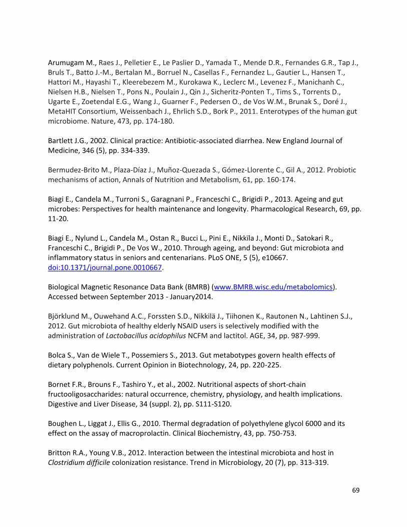
69
Arumugam M., Raes J., Pelletier E., Le Paslier D., Yamada T., Mende D.R., Fernandes G.R., Tap J., Bruls T., Batto J.-M., Bertalan M., Borruel N., Casellas F., Fernandez L., Gautier L., Hansen T., Hattori M., Hayashi T., Kleerebezem M., Kurokawa K., Leclerc M., Levenez F., Manichanh C., Nielsen H.B., Nielsen T., Pons N., Poulain J., Qin J., Sicheritz-Ponten T., Tims S., Torrents D., Ugarte E., Zoetendal E.G., Wang J., Guarner F., Pedersen O., de Vos W.M., Brunak S., Doré J., MetaHIT Consortium, Weissenbach J., Ehrlich S.D., Bork P., 2011. Enterotypes of the human gut microbiome. Nature, 473, pp. 174-180. Bartlett J.G., 2002. Clinical practice: Antibiotic-associated diarrhea. New England Journal of Medicine, 346 (5), pp. 334-339. Bermudez-Brito M., Plaza-Díaz J., Muñoz-Quezada S., Gómez-Llorente C., Gil A., 2012. Probiotic mechanisms of action, Annals of Nutrition and Metabolism, 61, pp. 160-174. Biagi E., Candela M., Turroni S., Garagnani P., Franceschi C., Brigidi P., 2013. Ageing and gut microbes: Perspectives for health maintenance and longevity. Pharmacological Research, 69, pp. 11-20. Biagi E., Nylund L., Candela M., Ostan R., Bucci L., Pini E., Nikkïla J., Monti D., Satokari R., Franceschi C., Brigidi P., De Vos W., 2010. Through ageing, and beyond: Gut microbiota and inflammatory status in seniors and centenarians. PLoS ONE, 5 (5), e10667. doi:10.1371/journal.pone.0010667. Biological Magnetic Resonance Data Bank (BMRB) (www.BMRB.wisc.edu/metabolomics). Accessed between September 2013 - January2014. Björklund M., Ouwehand A.C., Forssten S.D., Nikkilä J., Tiihonen K., Rautonen N., Lahtinen S.J., 2012. Gut microbiota of healthy elderly NSAID users is selectively modified with the administration of Lactobacillus acidophilus NCFM and lactitol. AGE, 34, pp. 987-999. Bolca S., Van de Wiele T., Possemiers S., 2013. Gut metabotypes govern health effects of dietary polyphenols. Current Opinion in Biotechnology, 24, pp. 220-225. Bornet F.R., Brouns F., Tashiro Y., et al., 2002. Nutritional aspects of short-chain fructooligosaccharides: natural occurrence, chemistry, physiology, and health implications. Digestive and Liver Disease, 34 (suppl. 2), pp. S111-S120. Boughen L., Liggat J., Ellis G., 2010. Thermal degradation of polyethylene glycol 6000 and its effect on the assay of macroprolactin. Clinical Biochemistry, 43, pp. 750-753. Britton R.A., Young V.B., 2012. Interaction between the intestinal microbiota and host in Clostridium difficile colonization resistance. Trend in Microbiology, 20 (7), pp. 313-319.
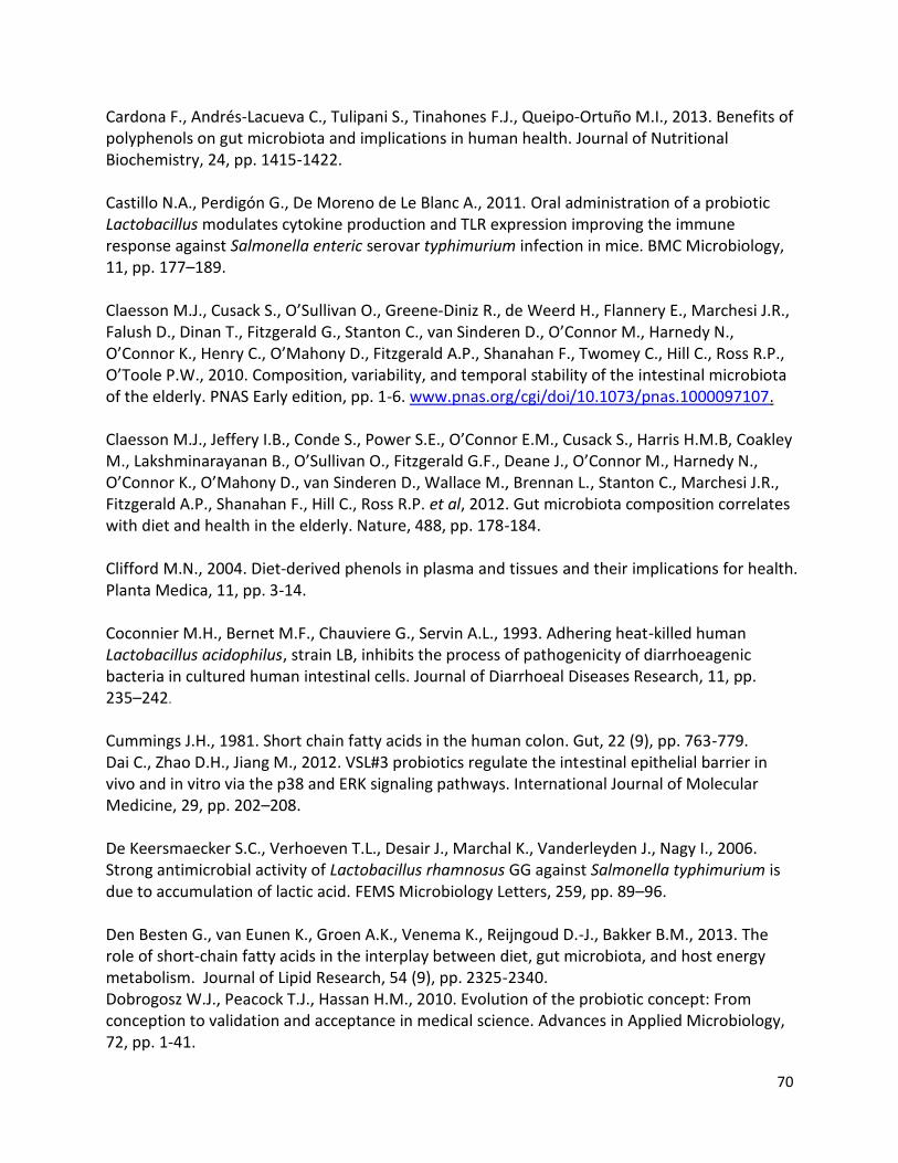
70
Cardona F., Andrés-Lacueva C., Tulipani S., Tinahones F.J., Queipo-Ortuño M.I., 2013. Benefits of polyphenols on gut microbiota and implications in human health. Journal of Nutritional Biochemistry, 24, pp. 1415-1422. Castillo N.A., Perdigón G., De Moreno de Le Blanc A., 2011. Oral administration of a probiotic Lactobacillus modulates cytokine production and TLR expression improving the immune response against Salmonella enteric serovar typhimurium infection in mice. BMC Microbiology, 11, pp. 177–189. Claesson M.J., Cusack S., O’Sullivan O., Greene-Diniz R., de Weerd H., Flannery E., Marchesi J.R., Falush D., Dinan T., Fitzgerald G., Stanton C., van Sinderen D., O’Connor M., Harnedy N., O’Connor K., Henry C., O’Mahony D., Fitzgerald A.P., Shanahan F., Twomey C., Hill C., Ross R.P., O’Toole P.W., 2010. Composition, variability, and temporal stability of the intestinal microbiota of the elderly. PNAS Early edition, pp. 1-6. www.pnas.org/cgi/doi/10.1073/pnas.1000097107. Claesson M.J., Jeffery I.B., Conde S., Power S.E., O’Connor E.M., Cusack S., Harris H.M.B, Coakley M., Lakshminarayanan B., O’Sullivan O., Fitzgerald G.F., Deane J., O’Connor M., Harnedy N., O’Connor K., O’Mahony D., van Sinderen D., Wallace M., Brennan L., Stanton C., Marchesi J.R., Fitzgerald A.P., Shanahan F., Hill C., Ross R.P. et al, 2012. Gut microbiota composition correlates with diet and health in the elderly. Nature, 488, pp. 178-184. Clifford M.N., 2004. Diet-derived phenols in plasma and tissues and their implications for health. Planta Medica, 11, pp. 3-14. Coconnier M.H., Bernet M.F., Chauviere G., Servin A.L., 1993. Adhering heat-killed human Lactobacillus acidophilus, strain LB, inhibits the process of pathogenicity of diarrhoeagenic bacteria in cultured human intestinal cells. Journal of Diarrhoeal Diseases Research, 11, pp. 235–242. Cummings J.H., 1981. Short chain fatty acids in the human colon. Gut, 22 (9), pp. 763-779. Dai C., Zhao D.H., Jiang M., 2012. VSL#3 probiotics regulate the intestinal epithelial barrier in vivo and in vitro via the p38 and ERK signaling pathways. International Journal of Molecular Medicine, 29, pp. 202–208. De Keersmaecker S.C., Verhoeven T.L., Desair J., Marchal K., Vanderleyden J., Nagy I., 2006. Strong antimicrobial activity of Lactobacillus rhamnosus GG against Salmonella typhimurium is due to accumulation of lactic acid. FEMS Microbiology Letters, 259, pp. 89–96. Den Besten G., van Eunen K., Groen A.K., Venema K., Reijngoud D.-J., Bakker B.M., 2013. The role of short-chain fatty acids in the interplay between diet, gut microbiota, and host energy metabolism. Journal of Lipid Research, 54 (9), pp. 2325-2340. Dobrogosz W.J., Peacock T.J., Hassan H.M., 2010. Evolution of the probiotic concept: From conception to validation and acceptance in medical science. Advances in Applied Microbiology, 72, pp. 1-41.
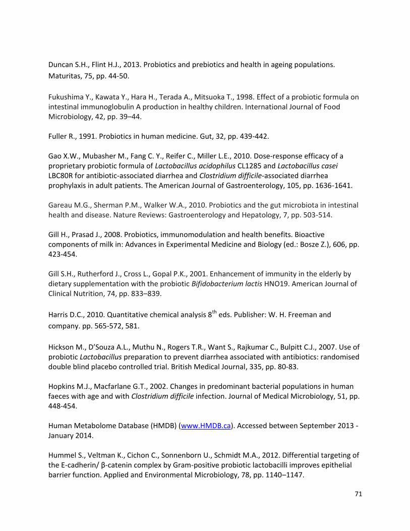
71
Duncan S.H., Flint H.J., 2013. Probiotics and prebiotics and health in ageing populations.
Maturitas, 75, pp. 44-50.
Fukushima Y., Kawata Y., Hara H., Terada A., Mitsuoka T., 1998. Effect of a probiotic formula on intestinal immunoglobulin A production in healthy children. International Journal of Food Microbiology, 42, pp. 39–44. Fuller R., 1991. Probiotics in human medicine. Gut, 32, pp. 439-442. Gao X.W., Mubasher M., Fang C. Y., Reifer C., Miller L.E., 2010. Dose-response efficacy of a proprietary probiotic formula of Lactobacillus acidophilus CL1285 and Lactobacillus casei LBC80R for antibiotic-associated diarrhea and Clostridium difficile-associated diarrhea prophylaxis in adult patients. The American Journal of Gastroenterology, 105, pp. 1636-1641. Gareau M.G., Sherman P.M., Walker W.A., 2010. Probiotics and the gut microbiota in intestinal health and disease. Nature Reviews: Gastroenterology and Hepatology, 7, pp. 503-514. Gill H., Prasad J., 2008. Probiotics, immunomodulation and health benefits. Bioactive components of milk in: Advances in Experimental Medicine and Biology (ed.: Bosze Z.), 606, pp. 423-454. Gill S.H., Rutherford J., Cross L., Gopal P.K., 2001. Enhancement of immunity in the elderly by dietary supplementation with the probiotic Bifidobacterium lactis HNO19. American Journal of Clinical Nutrition, 74, pp. 833–839.
Harris D.C., 2010. Quantitative chemical analysis 8th eds. Publisher: W. H. Freeman and
company. pp. 565-572, 581.
Hickson M., D’Souza A.L., Muthu N., Rogers T.R., Want S., Rajkumar C., Bulpitt C.J., 2007. Use of probiotic Lactobacillus preparation to prevent diarrhea associated with antibiotics: randomised double blind placebo controlled trial. British Medical Journal, 335, pp. 80-83. Hopkins M.J., Macfarlane G.T., 2002. Changes in predominant bacterial populations in human faeces with age and with Clostridium difficile infection. Journal of Medical Microbiology, 51, pp. 448-454. Human Metabolome Database (HMDB) (www.HMDB.ca). Accessed between September 2013 - January 2014. Hummel S., Veltman K., Cichon C., Sonnenborn U., Schmidt M.A., 2012. Differential targeting of the E-cadherin/ β-catenin complex by Gram-positive probiotic lactobacilli improves epithelial barrier function. Applied and Environmental Microbiology, 78, pp. 1140–1147.
72
Ibrahim F., Ruvio S., Granlund L., Salminen S., Viitanen M., Ouwehand A.C., 2010. Probiotics and immunosenescence: cheese as a carrier. FEMS Immunology and Medical Microbiology, 59 (1), pp. 53-59. Jacobs D.M., Deltimple N., van Velzen E., van Dorsten F.A., Bingham M., Vaughan E.E., van Duynhoven J., 2008. 1H NMR metabolite profiling of feces as a tool to assess the impact of nutrition on the human microbiome. NMR in Biomedicine, 21, pp. 615-626. Kaila M., Isolauri E., Soppi E., Virtanen E., Laine S., Arvilommi H., 1992. Enhancement of the circulating antibody secreting cell response in human diarrhea by a human Lactobacillus strain. Pediatric Research, 32 (2), pp. 141–144. Katz J.A., 2006. Probiotics for the prevention of antibiotic-associated diarrhea and Clostridium difficile diarrhea. Journal of Clinical Gastroenterology, 40 (3), pp. 249-255. Keller J.M., Surawicz C.M., 2014. Clostridium difficile infection in the elderly. Clinics in Geriatric Medicine, 30 (1), pp. 79-93. Kjeldahl K., Rasmussen M.A., Hasselbalch A.L., Kyvik K.O., Christiansen L., Rezzi S., Kochhar S., Sørensen T.I.A., Bro R., 2014. No genetic footprints of the fat mass and obesity associated (FTO) gene in human plasma 1H CPMG NMR metabolic profiles. Metabolomics, 10, pp. 132-140. Konishi Y., Kobayashi S., 2004. Transepithelial transport of chlorogenic acid, caffeic acid, and their colonic metabolites in intestinal Caco-2 cell monolayers. Journal of Agricultural and Food Chemistry, 52, pp. 2518-2526. Koprivnjak T., Peschel A., Gelb M.H., Liang N.S., Weiss J.P., 2002. Role of charge properties of bacterial envelope in bactericidal action of human group IIA phospholipase A2 against Staphylococcus aureus . Journal of Biological Chemistry, 277, pp. 47636–47644.
Kupiec T., 2004. Quality control analytical methods: Gas chromatography. International Journal
of Pharmaceutical Compounding, 8 (4), pp. 305-309.
Lahtinen S., Forssten S., Aakko J., Granlund L., Rautonen N., Salminen S., Viitanen M., Ouwehand A.C., 2012. Probiotic cheese containing Lactobacillus rhamnosus HN001 and Lactobacillus acidophilus NCFM® modifies subpopulations of fecal lactobacilli and Clostridium difficile in the elderly. AGE, 34 (1), pp. 133-143. Larsen C.N., Nielsen S., Kæstel P., Brockmann E., Bennedsen M., Christensen H.R., Eskesen D.C., Jacobsen B.L., Michaelsen K.F., 2006. Dose-response study of probiotic bacteria Bifidobacterium animalis subsp. lactis BB-12 and Lactobacillus paracasei subsp. paracasei CRL-341 in healthy young adults. European Journal of Clinical Nutrition, 60, pp. 1284-1293.
73
Le Gall G., Noor S.O., Ridgway K., Scovell L., Jamieson C., Johnson I.T., Colquhoun I.J., Kemsley E.K., Narbad A., 2011. Metabolomics of fecal extracts detects altered metabolic activity of gut microbiota in ulcerative colitis and irritable bowel syndrome. Journal of Proteome Research, 10, pp. 4208-4218. LeBlanc J.G., Milani C., de Giori G.S., Sesma F., van Sinderen D., Ventura M., 2013. Bacteria as vitamin suppliers to their host: a gut microbiota perspective. Current Opinion in Biotechnology, 24, pp. 160-168. Lessa F.C., Gould C.V., McDonald L.C., 2012. Current status of Clostridium difficile infection epidemiology. Clinical Infectious Diseases, 55 (suppl. 2), pp. S65-S70. Liu Y., Fatheree N.Y., Mangalat N., Rhoads J.M., 2012. Lactobacillus reuteri strains reduce incidence and severity of experimental necrotizing enterocolitis via modulation of TLR4 and NF-κB signaling in the intestine. American Journal of Physiology, Gastrointestinal and Liver Physiology, 302, pp. 608–617.
Macfarlane G.T., Macfarlane S., 2012. Bacteria, Colonic fermentation, and Gastrointestinal
health. Journal of AOAC International, 95 (1), pp. 50-60.
Mäkivuokko H., Nurmi J., Nurminen PP., Stowell J., Rautonen N., 2005. In Vitro effects on polydextrose by colonic bacteria and Caco-2 cell cyclooxygenase gene expression. Nutrition and Cancer, 51 (1), pp. 94-104. Mäkivuokko H., Tiihonen K., Tynkkynen S., Paulin L., Rautonen N., 2010. The effect of age and non-steroidal anti-inflammatory drugs on human intestinal microbiota composition. British Journal of Nutrition, 103, pp. 227-234. Makras L., Triantafyllou V., Fayol-Messaoudi D., Adriany T., Zoumpopoulou G., Tsakalidou E., Servin A., DeVuyst L., 2006. Kinetic analysis of the antibacterial activity of probiotic lactobacilli towards Salmonella enterica serovar typhimurium reveals a role for lactic acid and other inhibitory compounds. Research in Microbiology, 157, pp. 241–247. Mariat D., Firmesse O., Levenez F., Guimarăes V.D., Sokol H., Doré J., Corthier G., Furet J.-P., 2009. The Firmicutes/Bacteroidetes ratio of the human microbiota changes with age. BMC Microbiology, 9, pp. 123-128. Marquet P., Duncan S.H., Chassard C., Bernalier-Donadille A., Flint H.J., 2009. Lactate has the potential to promote hydrogen sulphide formation in the human colon. FEMS Microbiology Letters, 299, pp. 128-134.
74
Mättö J., Fondén R., Tolvanen T., von Wright A., Vilpponen-Salmela T., Satokari R., Saarela M., 2006. Intestinal survival and persistence of probiotic Lactobacillus and Bifidobacterium strains administered in triple-strain yoghurt. International Dairy Journal, 16, pp. 1174-1180. McFarland L.V., 2006. Meta-analysis of probiotics for the prevention of antibiotic associated diarrhea and the treatment of Clostridium difficile disease. American Journal of Gastroenterology, 101, pp. 812-822. Müller C.A., Autenrieth I.B., Peschel A., 2005. Innate defenses of the intestinal epithelial barrier. Cellular and Molecular Life Science, 62, pp. 1297–1307. Nagao F., Nakayama M., Muto T., Okumura K., 2000. Effects of a fermented milk drink containing Lactobacillus casei strain Shirota on the immune system in healthy human subjects. Bioscience, Biotechnology, and Biochemistry, 64 (12), pp. 2706–2708. Ndagijimana M., Laghi L., Vitali B., Placucci G., Brigidi P., Guerzoni E., 2009. Effect of a symbiotic food consumption on human gut metabolic profiles evaluated by 1H Nuclear Magnetic Resonance spectroscopy. International Journal of Food Microbiology, 134, pp. 147-153. Ouwehand A.C., ten Bruggencate S.J.M., Schonewille A.J., Alhoniemi H., Forssten S.D., Bovee-Oudenhoven I.M.J., 2014. Lactobacillus acidophilus supplementation in human subjects and their resistance to enterotoxigenic Escherichia coli infection. British Journal of Nutrition, 111 (3), pp. 465-473. Ouwehand A.C., Tiihonen K., Saarinen M., Putaala H., Rautonen N., 2009. Influence of a combination of Lactobacillus acidophilus NCFM and lactitol on healthy elderly: intestinal and immune parameters. British Journal of Nutrition, 101, pp. 367-375. Parkar S.G., Trower T.M., Stevenson D.E., 2013. Fecal microbial metabolism of polyphenols and its effects on human gut microbiota. Anaerobe, 23, pp. 12-19. Pena J.A., Versalovic J., 2003. Lactobacillus rhamnosus GG decreases TNF-α production in lipopolysaccharide-activated murine macrophages by a contact-independent mechanism. Cell Microbiology, 5, pp. 277-285.
Quigley E.M.M., 2011. Gut microbiota and the role of probiotics in therapy. Current Opinion in
Pharmacology, 11, pp. 593-603.
Rajilić-Stojanović M., Heilig H.G.H.J., Molenaar D., Kajander K., Surakka A., Smidt H., de Vos W.M., 2009. Development and application of the human intestinal tract chip, a phylogenetic microarray: analysis of universally conserved phylotypes in the abundant microbiota of young and elderly adults. Environmental Microbiology, 11 (7), pp. 1736-1751.
75
Saad N., Delattre C., Urdaci M., Schmitter J.M., Bressollier P., 2013. An overview of the last advances in probiotic and prebiotic field. LWT – Food Science and Technology, 50, pp. 1-16. Schiffrin E.J., Blum S., 2002. Interactions between the microbiota and the intestinal mucosa. European Journal of Clinical Nutrition, 56, pp. 60–64. Sealy L., Chalkley R., 1978. The effect of sodium butyrate on histone modification. Cell, 14 (1), pp. 115-121. Smith E.A., Macfarlane G.T., 1997. Dissimilatory amino acid metabolism in human colonic bacteria. Anaerobe, 3, pp. 327-337.
Tiihonen K., Ouwehand A.C., Rautonen, N., 2010. Human intestinal microbiota and healthy
ageing. Ageing Research Reviews, 9, pp. 107-116.
Tiihonen K., Tynkkynen S., Ouwehand A., Ahlroos T., Rautonen N., 2008. The effect of ageing with and without non-steroidal anti-inflammatory drugs on gastrointestinal microbiology and immunology. British Journal of Nutrition, 100, pp. 130-137. Tzounis X., Rodriguez-Mateos A., Vulevic J., Gibson G.R., Kwik-Uribe C., Spencer J.P., 2011. Prebiotic evaluation of cocoa-derived flavanols in healthy humans by using a randomized, controlled, double-blind, crossover intervention study. American Journal of Clinical Nutrition, 93, pp. 62-72. VanGuilder H.D., Vrana K.E., Freeman W.M., 2008. Twenty-five years of quantitative PCR for gene expression analysis. BioTechniques, 44 (5), pp. 619-626. Wang S., Zhu H., Lu C., Kang Z., Luo Y., Feng L., Lu X., 2012. Fermented milk supplemented with probiotics and prebiotics can effectively alter the intestinal microbiota and immunity of host animals. Journal of Dairy Science, 95 (9), pp. 4813-4822. Weber D.J., Anderson D.J., Sexton D.J., Rutala W.A., 2013. Role of the environment in the transmission of Clostridium difficile in health care facilities. American Journal of infection Control, 41 (5) (supplement), pp. S105-S110. Wong J.M.W, de Souza R., Kendall C.W.C., Emam A., Jenkins D.J.A., 2006. Colonic health: Fermentation and short chain fatty acids. Journal of Clinical Gastroenterology, 40, pp. 235-243. Woodmansey E.J., McMurdo M.E.T., Macfarlane G.T., Macfarlane S., 2004. Comparison of compositions and metabolic activities of fecal microbiotas in young adults and in antibiotic-treated and non-antibiotic-treated elderly subjects. Applied and Environmental Microbiology, 70 (10), pp. 6113-6122.
76
Wu J., An Y., Yao J., Wang Y., Tang H., 2010. An optimised sample preparation method for NMR-based faecal metabonomic analysis. Analyst, 135, pp. 1023-1030. Zhang L., Li N., Caicedo R., Neu J., 2005. Alive and dead Lactobacillus rhamnosus GG decrease tumor necrosis factor-a-induced interleukin-8 production in Caco-2 cells. Journal of Nutrition, 135, pp. 1752-1756. Zheng X., Qiu Y., Zhong W., Baxter S., Su M., Li Q., Xie G., Ore B.M., Qiao S., Spencer M.D., Zeisel S.H., Zhou Z., Zhao A., Jia W., 2013. A targeted metabolomic protocol for short-chain fatty acids and branched-chain amino acids. Metabolomics, 9, pp. 818-827. Zhu D.J., Chen X.W., Wu J.H., Ju Y.L., Feng J., Lu G.S., Ouyang M.Z., Ren B.J., Li Y., 2012. Effect of perioperative intestinal probiotics on intestinal flora and immune function in patients with colorectal cancer. Journal of Southern Medical University, 32 (8), pp. 1190–1193.
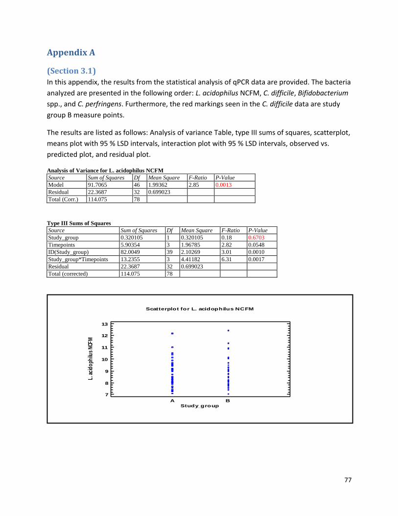
77
Appendix A
(Section 3.1)
In this appendix, the results from the statistical analysis of qPCR data are provided. The bacteria
analyzed are presented in the following order: L. acidophilus NCFM, C. difficile, Bifidobacterium
spp., and C. perfringens. Furthermore, the red markings seen in the C. difficile data are study
group B measure points.
The results are listed as follows: Analysis of variance Table, type III sums of squares, scatterplot,
means plot with 95 % LSD intervals, interaction plot with 95 % LSD intervals, observed vs.
predicted plot, and residual plot.
Analysis of Variance for L. acidophilus NCFM
Source Sum of Squares Df Mean Square F-Ratio P-Value
Model 91.7065 46 1.99362 2.85 0.0013
Residual 22.3687 32 0.699023
Total (Corr.) 114.075 78
Type III Sums of Squares
Source Sum of Squares Df Mean Square F-Ratio P-Value
Study_group 0.320105 1 0.320105 0.18 0.6703
Timepoints 5.90354 3 1.96785 2.82 0.0548
ID(Study_group) 82.0049 39 2.10269 3.01 0.0010
Study_group*Timepoints 13.2355 3 4.41182 6.31 0.0017
Residual 22.3687 32 0.699023
Total (corrected) 114.075 78
A B
Study_group
Scatterplot for L. acidophilus NCFM
7
8
9
10
11
12
13
L. a
cid
oph
ilus
NCF
M
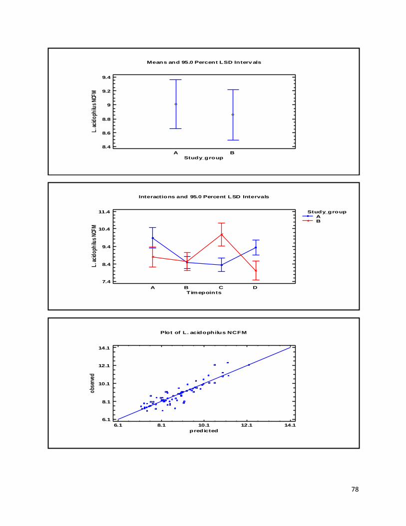
78
A B
Means and 95.0 Percent LSD Interv als
Study_group
8.4
8.6
8.8
9
9.2
9.4
L. a
cid
oph
ilus
NCF
M
Interactions and 95.0 Percent LSD Intervals
Timepoints
7.4
8.4
9.4
10.4
11.4
L. a
cid
oph
ilus
NCF
M
A B C D
Study_groupAB
Plot of L. acidophilus NCFM
6.1 8.1 10.1 12.1 14.1
predicted
6.1
8.1
10.1
12.1
14.1
obs
erve
d
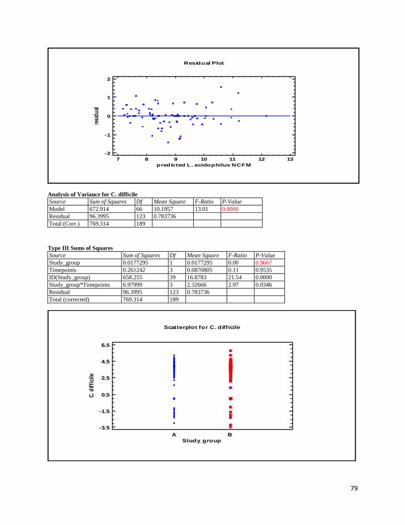
79
Analysis of Variance for C. difficile
Source Sum of Squares Df Mean Square F-Ratio P-Value
Model 672.914 66 10.1957 13.01 0.0000
Residual 96.3995 123 0.783736
Total (Corr.) 769.314 189
Type III Sums of Squares
Source Sum of Squares Df Mean Square F-Ratio P-Value
Study_group 0.0177295 1 0.0177295 0.00 0.9667
Timepoints 0.261242 3 0.0870805 0.11 0.9535
ID(Study_group) 658.255 39 16.8783 21.54 0.0000
Study_group*Timepoints 6.97999 3 2.32666 2.97 0.0346
Residual 96.3995 123 0.783736
Total (corrected) 769.314 189
7 8 9 10 11 12 13
predicted L. acidophilus NCFM
Residual Plot
-2
-1
0
1
2
resi
du
al
A B
Study_group
Scatterplot for C. difficile
-3.5
-1.5
0.5
2.5
4.5
6.5
C. d
iffi
cile
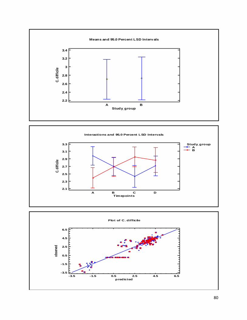
80
A B
Means and 95.0 Percent LSD Interv als
Study_group
2.2
2.4
2.6
2.8
3
3.2
3.4
C. d
iffi
cile
Interactions and 95.0 Percent LSD Intervals
Timepoints
2.1
2.3
2.5
2.7
2.9
3.1
3.3
C. d
iffic
ile
A B C D
Study_groupAB
Plot of C. difficile
-3.5 -1.5 0.5 2.5 4.5 6.5
predicted
-3.5
-1.5
0.5
2.5
4.5
6.5
obs
erve
d
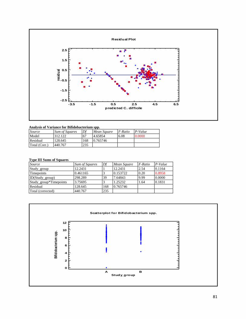
81
Analysis of Variance for Bifidobacterium spp.
Source Sum of Squares Df Mean Square F-Ratio P-Value
Model 312.122 67 4.65854 6.08 0.0000
Residual 128.645 168 0.765746
Total (Corr.) 440.767 235
Type III Sums of Squares
Source Sum of Squares Df Mean Square F-Ratio P-Value
Study_group 12.2431 1 12.2431 2.54 0.1164
Timepoints 0.461165 3 0.153722 0.20 0.8958
ID(Study_group) 298.289 39 7.64843 9.99 0.0000
Study_group*Timepoints 3.75695 3 1.25232 1.64 0.1831
Residual 128.645 168 0.765746
Total (corrected) 440.767 235
-3.5 -1.5 0.5 2.5 4.5 6.5
predicted C. difficile
Residual Plot
-2.5
-1.5
-0.5
0.5
1.5
2.5
res
idu
al
A B
Study_group
Scatterplot for Bifidobacterium spp.
0
2
4
6
8
10
12
Bifi
dob
acte
rium
spp
.
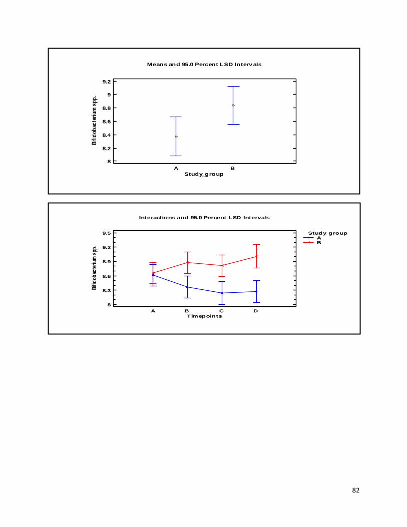
82
A B
Means and 95.0 Percent LSD Interv als
Study_group
8
8.2
8.4
8.6
8.8
9
9.2
Bifi
dob
acte
rium
spp
.
Interactions and 95.0 Percent LSD Intervals
Timepoints
8
8.3
8.6
8.9
9.2
9.5
Bifi
dob
acte
rium
spp
.
A B C D
Study_groupAB
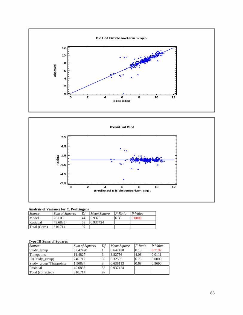
83
Analysis of Variance for C. Perfringens
Source Sum of Squares Df Mean Square F-Ratio P-Value
Model 261.03 44 5.9325 6.33 0.0000
Residual 49.6835 53 0.937424
Total (Corr.) 310.714 97
Type III Sums of Squares
Source Sum of Squares Df Mean Square F-Ratio P-Value
Study_group 0.647428 1 0.647428 0.13 0.7192
Timepoints 11.4827 3 3.82756 4.08 0.0111
ID(Study_group) 246.712 39 6.32595 6.75 0.0000
Study_group*Timepoints 1.90834 3 0.636113 0.68 0.5690
Residual 49.6835 53 0.937424
Total (corrected) 310.714 97
Plot of Bifidobacterium spp.
0 2 4 6 8 10 12
predicted
0
2
4
6
8
10
12
obs
erve
d
0 2 4 6 8 10 12
predicted Bifidobacterium spp.
Residual Plot
-7.5
-4.5
-1.5
1.5
4.5
7.5
resi
du
al
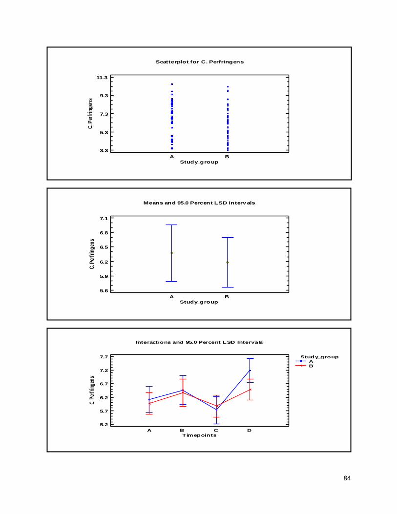
84
A B
Study_group
Scatterplot for C. Perfringens
3.3
5.3
7.3
9.3
11.3
C. P
erfr
ing
ens
A B
Means and 95.0 Percent LSD Interv als
Study_group
5.6
5.9
6.2
6.5
6.8
7.1
C. P
erfr
ing
ens
Interactions and 95.0 Percent LSD Intervals
Timepoints
5.2
5.7
6.2
6.7
7.2
7.7
C. P
erfr
ing
ens
A B C D
Study_groupAB
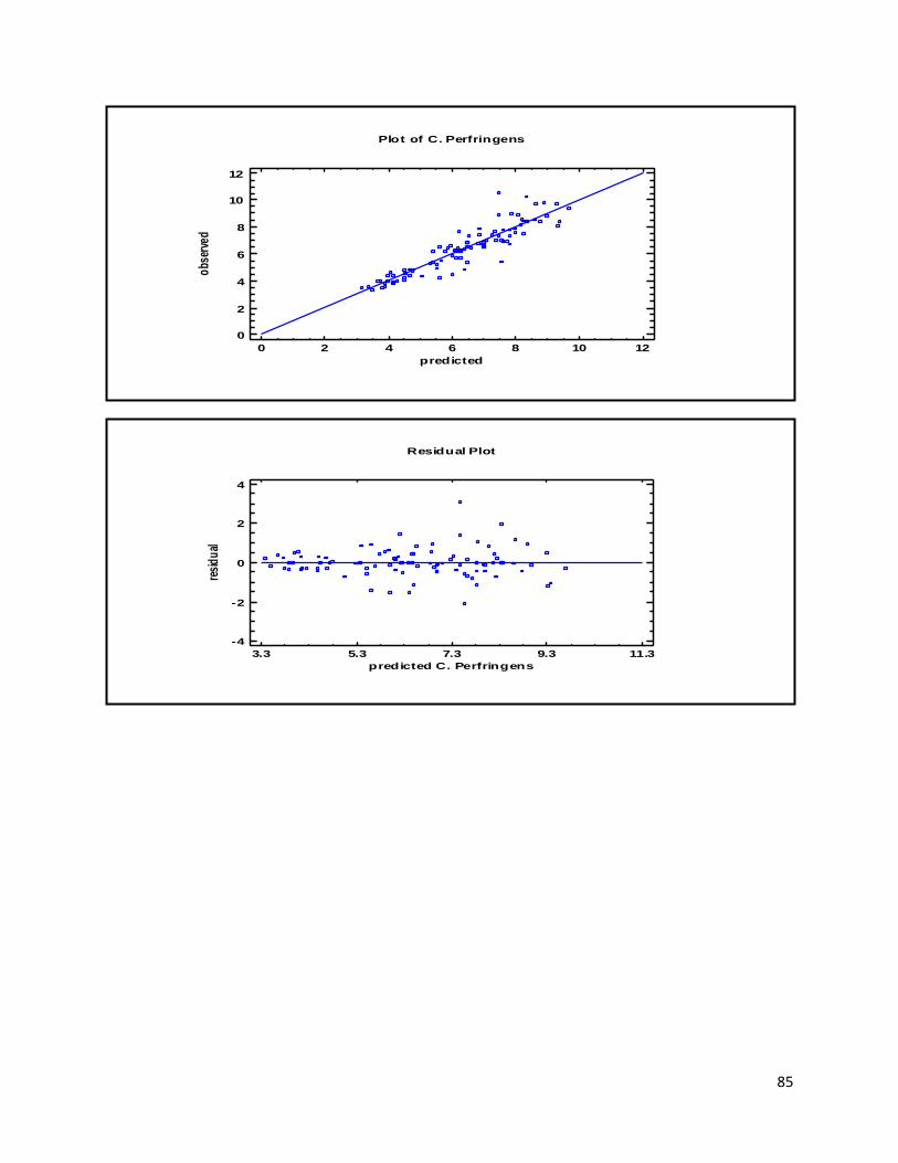
85
Plot of C. Perfringens
0 2 4 6 8 10 12
predicted
0
2
4
6
8
10
12
obs
erve
d
3.3 5.3 7.3 9.3 11.3
predicted C. Perfringens
Residual Plot
-4
-2
0
2
4
resi
du
al
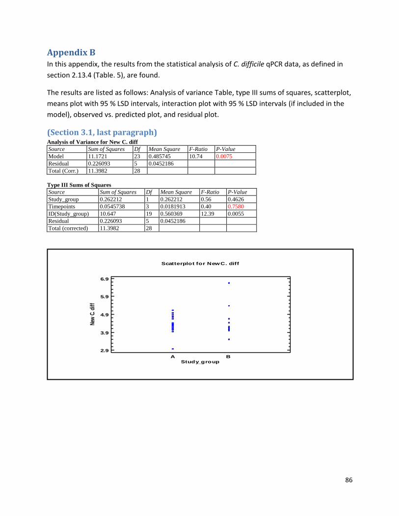
86
Appendix B In this appendix, the results from the statistical analysis of C. difficile qPCR data, as defined in
section 2.13.4 (Table. 5), are found.
The results are listed as follows: Analysis of variance Table, type III sums of squares, scatterplot,
means plot with 95 % LSD intervals, interaction plot with 95 % LSD intervals (if included in the
model), observed vs. predicted plot, and residual plot.
(Section 3.1, last paragraph) Analysis of Variance for New C. diff
Source Sum of Squares Df Mean Square F-Ratio P-Value
Model 11.1721 23 0.485745 10.74 0.0075
Residual 0.226093 5 0.0452186
Total (Corr.) 11.3982 28
Type III Sums of Squares
Source Sum of Squares Df Mean Square F-Ratio P-Value
Study_group 0.262212 1 0.262212 0.56 0.4626
Timepoints 0.0545738 3 0.0181913 0.40 0.7580
ID(Study_group) 10.647 19 0.560369 12.39 0.0055
Residual 0.226093 5 0.0452186
Total (corrected) 11.3982 28
A B
Study_group
Scatterplot for New C. diff
2.9
3.9
4.9
5.9
6.9
New
C. d
iff
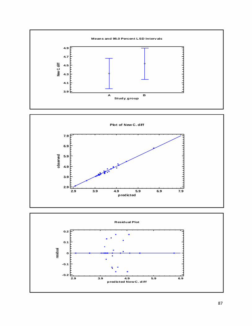
87
A B
Means and 95.0 Percent LSD Interv als
Study_group
3.9
4.1
4.3
4.5
4.7
4.9
New
C. d
iff
Plot of New C. diff
2.9 3.9 4.9 5.9 6.9 7.9
predicted
2.9
3.9
4.9
5.9
6.9
7.9
ob
ser
ved
2.9 3.9 4.9 5.9 6.9
predicted New C. diff
Residual Plot
-0.2
-0.1
0
0.1
0.2
resi
du
al

88
Analysis of Variance for New C. diff
Source Sum of Squares Df Mean Square F-Ratio P-Value
Model 0.830607 7 0.118658 0.24 0.9714
Residual 10.5676 21 0.50322
Total (Corr.) 11.3982 28
Type III Sums of Squares
Source Sum of Squares Df Mean Square F-Ratio P-Value
Study_group 0.00000878938 1 0.00000878938 0.00 0.9967
Timepoints 0.324602 3 0.108201 0.22 0.8849
Study_group*Timepoints 0.305493 3 0.101831 0.20 0.8936
Residual 10.5676 21 0.50322
Total (corrected) 11.3982 28
A B C D
Timepoints
Scatterplot for New C. diff
2.9
3.9
4.9
5.9
6.9
New
C.
dif
f
A B
Means and 95.0 Percent LSD Interv als
Study_group
4
4.2
4.4
4.6
4.8
New
C.
dif
f
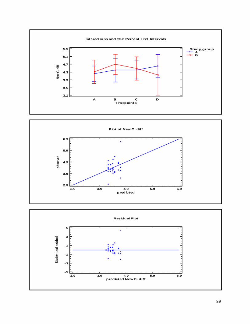
89
Interactions and 95.0 Percent LSD Intervals
Timepoints
3.1
3.5
3.9
4.3
4.7
5.1
5.5
New
C. d
iff
A B C D
Study_groupAB
Plot of New C. diff
2.9 3.9 4.9 5.9 6.9
predicted
2.9
3.9
4.9
5.9
6.9
obs
erve
d
2.9 3.9 4.9 5.9 6.9
predicted New C. diff
Residual Plot
-5
-3
-1
1
3
5
Stu
den
tize
d r
esid
ual
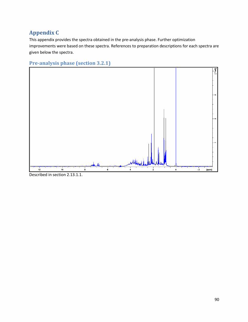
90
Appendix C This appendix provides the spectra obtained in the pre-analysis phase. Further optimization
improvements were based on these spectra. References to preparation descriptions for each spectra are
given below the spectra.
Pre-analysis phase (section 3.2.1)
Described in section 2.13.1.1.
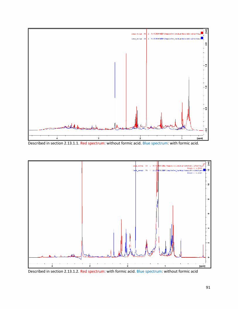
91
Described in section 2.13.1.1. Red spectrum: without formic acid. Blue spectrum: with formic acid.
Described in section 2.13.1.2. Red spectrum: with formic acid. Blue spectrum: without formic acid
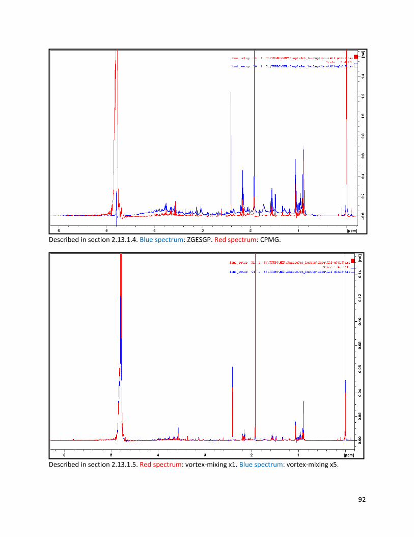
92
Described in section 2.13.1.4. Blue spectrum: ZGESGP. Red spectrum: CPMG.
Described in section 2.13.1.5. Red spectrum: vortex-mixing x1. Blue spectrum: vortex-mixing x5.
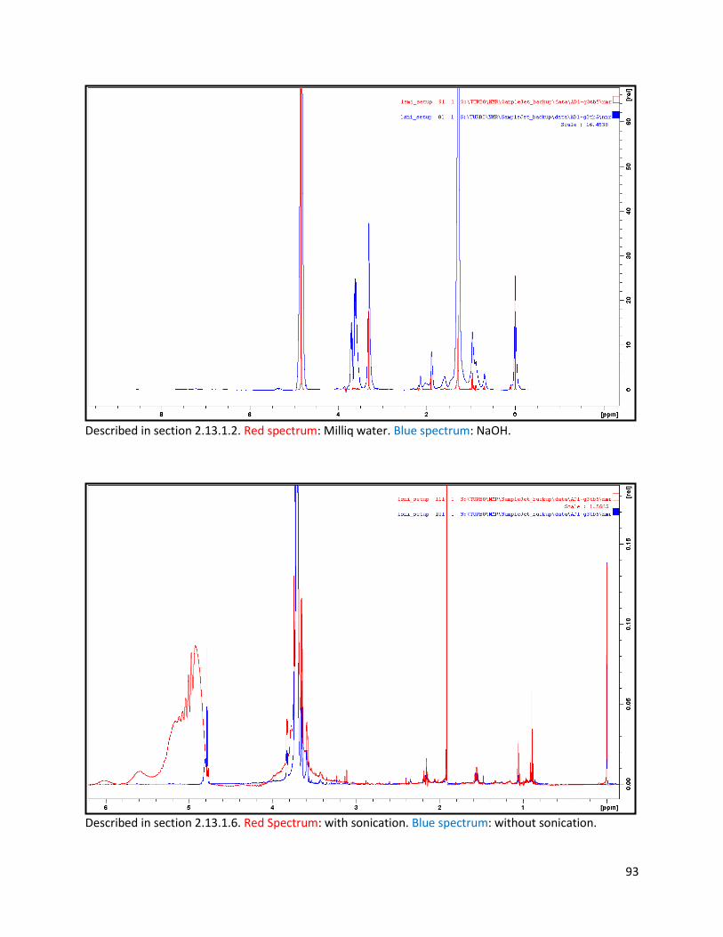
93
Described in section 2.13.1.2. Red spectrum: Milliq water. Blue spectrum: NaOH.
Described in section 2.13.1.6. Red Spectrum: with sonication. Blue spectrum: without sonication.
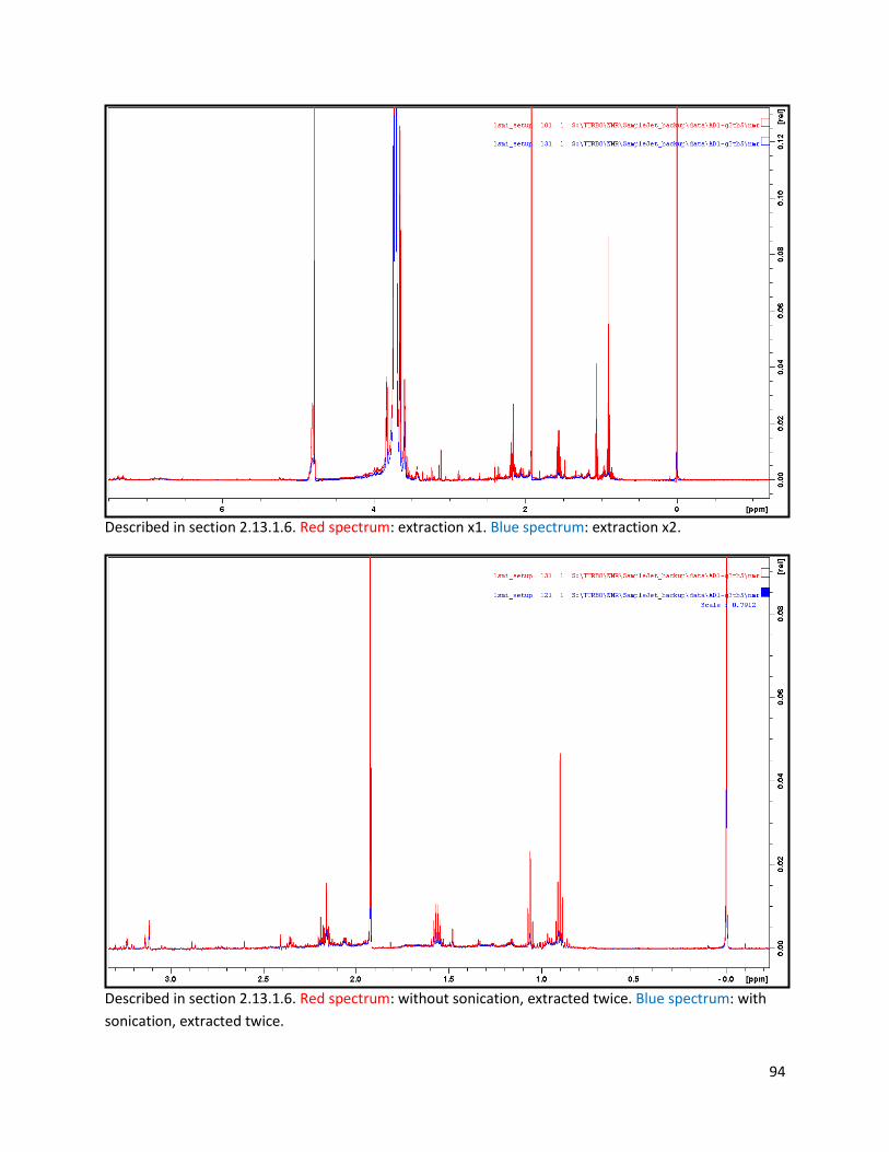
94
Described in section 2.13.1.6. Red spectrum: extraction x1. Blue spectrum: extraction x2.
Described in section 2.13.1.6. Red spectrum: without sonication, extracted twice. Blue spectrum: with
sonication, extracted twice.
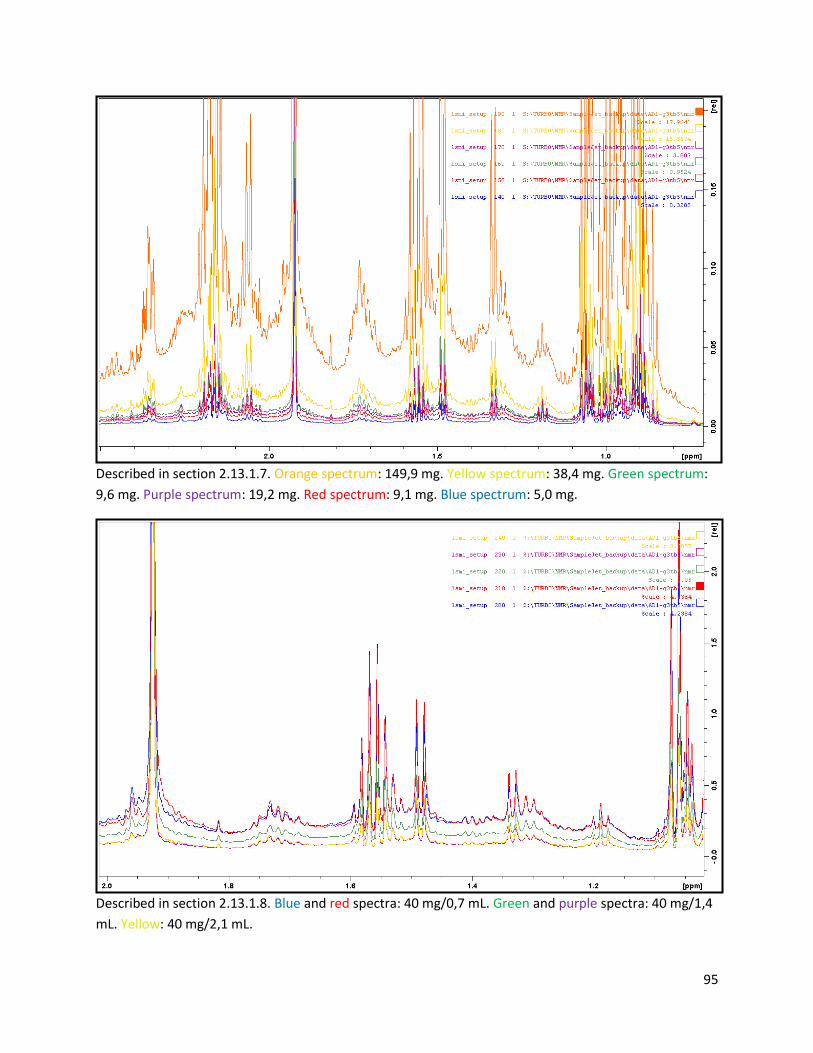
95
Described in section 2.13.1.7. Orange spectrum: 149,9 mg. Yellow spectrum: 38,4 mg. Green spectrum:
9,6 mg. Purple spectrum: 19,2 mg. Red spectrum: 9,1 mg. Blue spectrum: 5,0 mg.
Described in section 2.13.1.8. Blue and red spectra: 40 mg/0,7 mL. Green and purple spectra: 40 mg/1,4
mL. Yellow: 40 mg/2,1 mL.
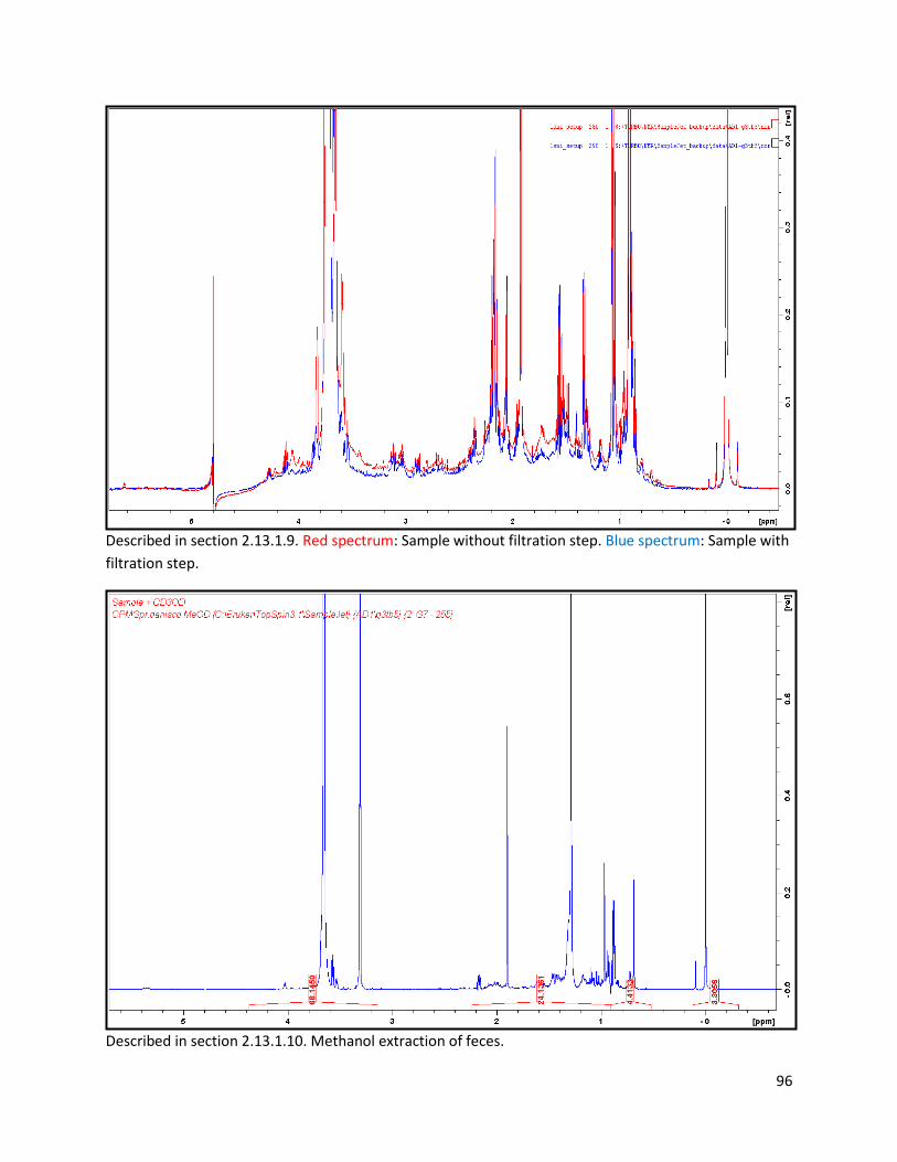
96
Described in section 2.13.1.9. Red spectrum: Sample without filtration step. Blue spectrum: Sample with
filtration step.
Described in section 2.13.1.10. Methanol extraction of feces.
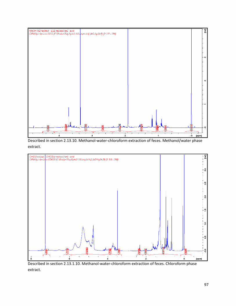
97
Described in section 2.13.10. Methanol-water-chloroform extraction of feces. Methanol/water phase
extract.
Described in section 2.13.1.10. Methanol-water-chloroform extraction of feces. Chloroform phase
extract.
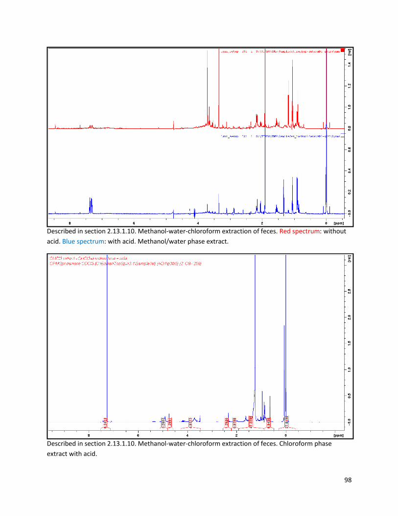
98
Described in section 2.13.1.10. Methanol-water-chloroform extraction of feces. Red spectrum: without
acid. Blue spectrum: with acid. Methanol/water phase extract.
Described in section 2.13.1.10. Methanol-water-chloroform extraction of feces. Chloroform phase
extract with acid.
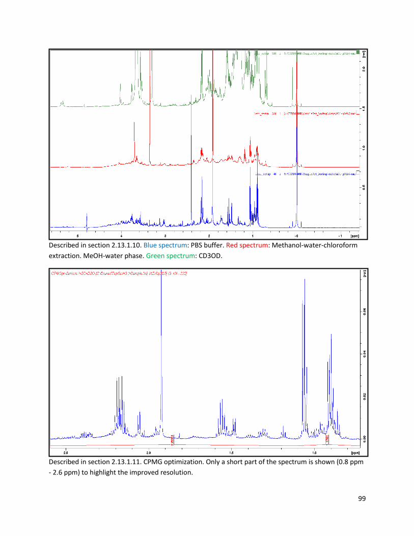
99
Described in section 2.13.1.10. Blue spectrum: PBS buffer. Red spectrum: Methanol-water-chloroform
extraction. MeOH-water phase. Green spectrum: CD3OD.
Described in section 2.13.1.11. CPMG optimization. Only a short part of the spectrum is shown (0.8 ppm
- 2.6 ppm) to highlight the improved resolution.
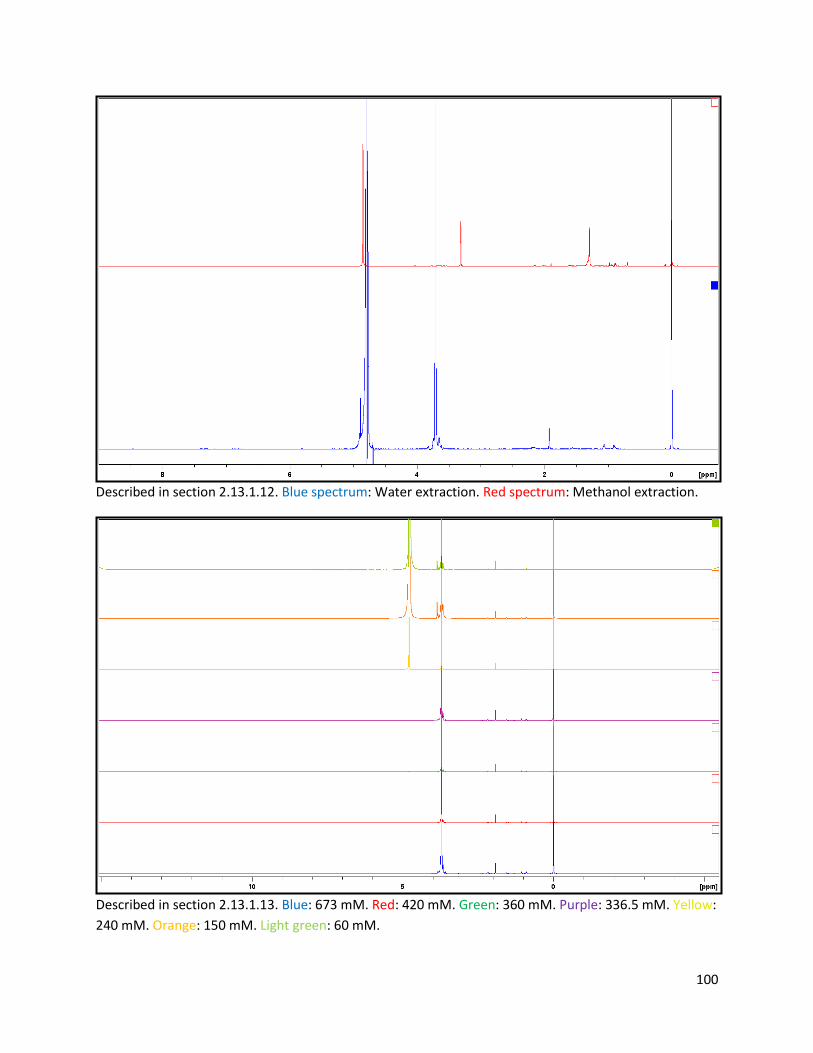
100
Described in section 2.13.1.12. Blue spectrum: Water extraction. Red spectrum: Methanol extraction.
Described in section 2.13.1.13. Blue: 673 mM. Red: 420 mM. Green: 360 mM. Purple: 336.5 mM. Yellow:
240 mM. Orange: 150 mM. Light green: 60 mM.
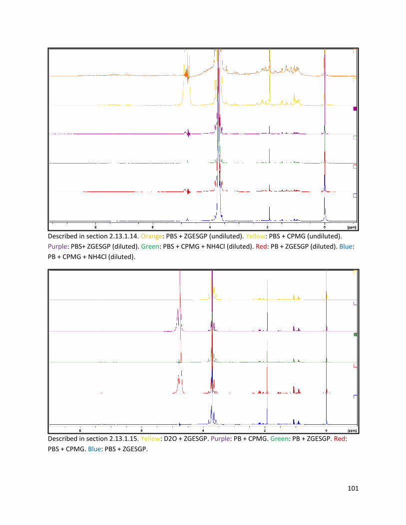
101
Described in section 2.13.1.14. Orange: PBS + ZGESGP (undiluted). Yellow: PBS + CPMG (undiluted).
Purple: PBS+ ZGESGP (diluted). Green: PBS + CPMG + NH4Cl (diluted). Red: PB + ZGESGP (diluted). Blue:
PB + CPMG + NH4Cl (diluted).
Described in section 2.13.1.15. Yellow: D2O + ZGESGP. Purple: PB + CPMG. Green: PB + ZGESGP. Red:
PBS + CPMG. Blue: PBS + ZGESGP.
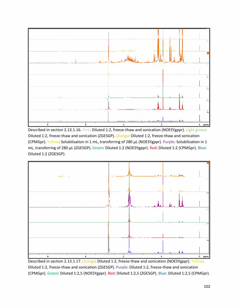
102
Described in section 2.13.1.16. Pink: Diluted 1:2, freeze-thaw and sonication (NOESYgppr). Light green:
Diluted 1:2, freeze-thaw and sonication (ZGESGP). Orange: Diluted 1:2, freeze-thaw and sonication
(CPMGpr). Yellow: Solubilisation in 1 mL, transferring of 280 μL (NOESYgppr). Purple: Solubilisation in 1
mL, transferring of 280 μL (ZGESGP). Green: Diluted 1:2 (NOESYgppr). Red: Diluted 1:2 (CPMGpr). Blue:
Diluted 1:2 (ZGESGP).
Described in section 2.13.1.17. Orange: Diluted 1:2, freeze-thaw and sonication (NOESYgppr). Yellow:
Diluted 1:2, freeze-thaw and sonication (ZGESGP). Purple: Diluted 1:2, freeze-thaw and sonication
(CPMGpr). Green: Diluted 1:2,5 (NOESYgppr). Red: Diluted 1:2,5 (ZGESGP). Blue: Diluted 1:2,5 (CPMGpr).
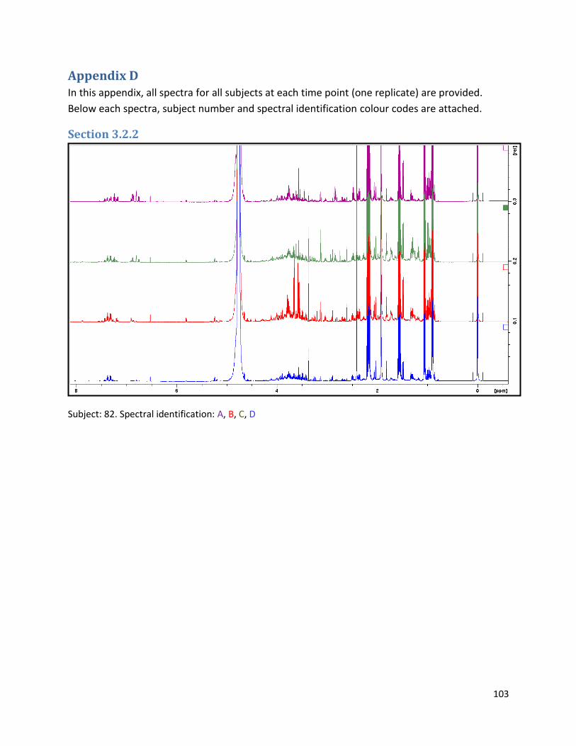
103
Appendix D In this appendix, all spectra for all subjects at each time point (one replicate) are provided.
Below each spectra, subject number and spectral identification colour codes are attached.
Section 3.2.2
Subject: 82. Spectral identification: A, B, C, D
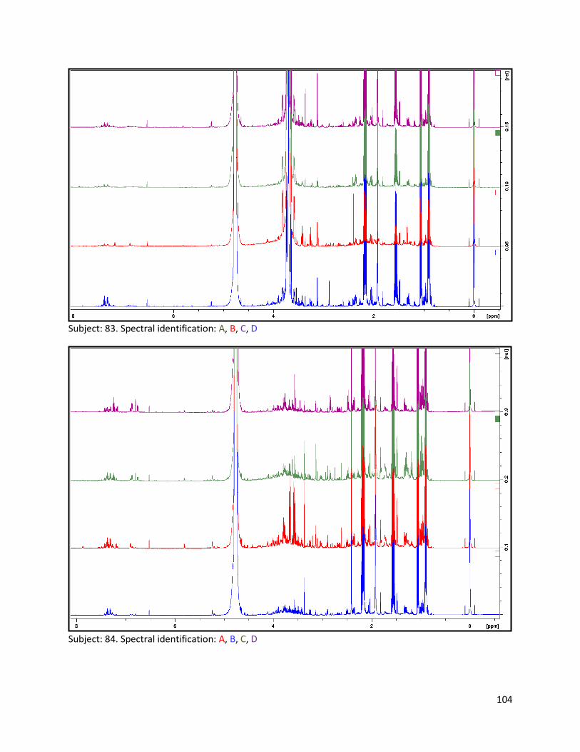
104
Subject: 83. Spectral identification: A, B, C, D
Subject: 84. Spectral identification: A, B, C, D
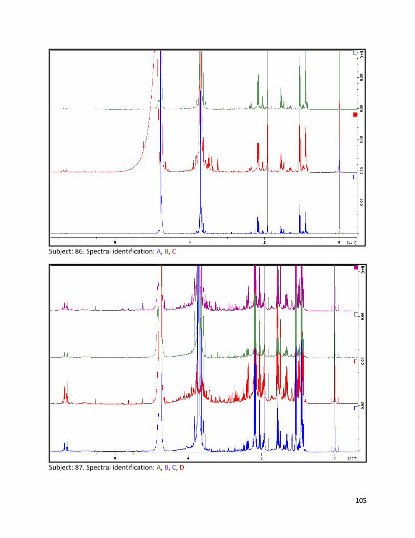
105
Subject: 86. Spectral identification: A, B, C
Subject: 87. Spectral identification: A, B, C, D
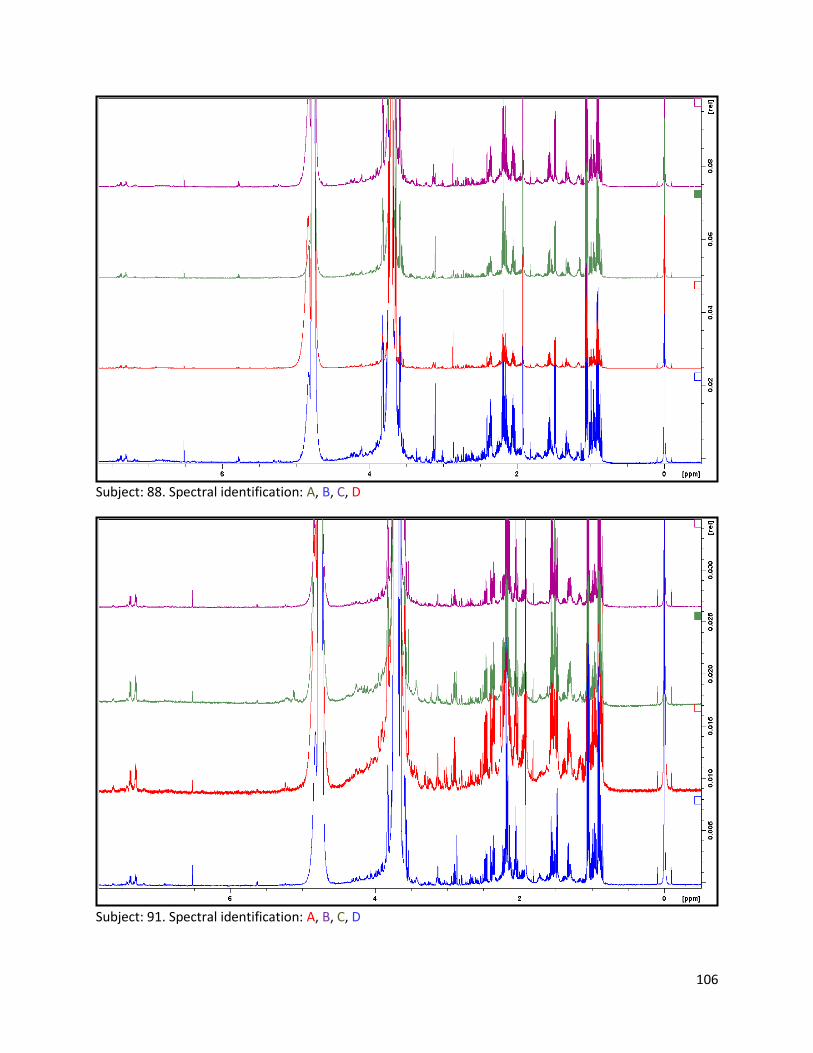
106
Subject: 88. Spectral identification: A, B, C, D
Subject: 91. Spectral identification: A, B, C, D
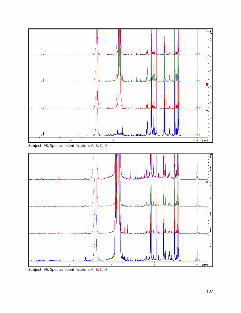
107
Subject: 93. Spectral identification: A, B, C, D
Subject: 95. Spectral identification: A, B, C, D
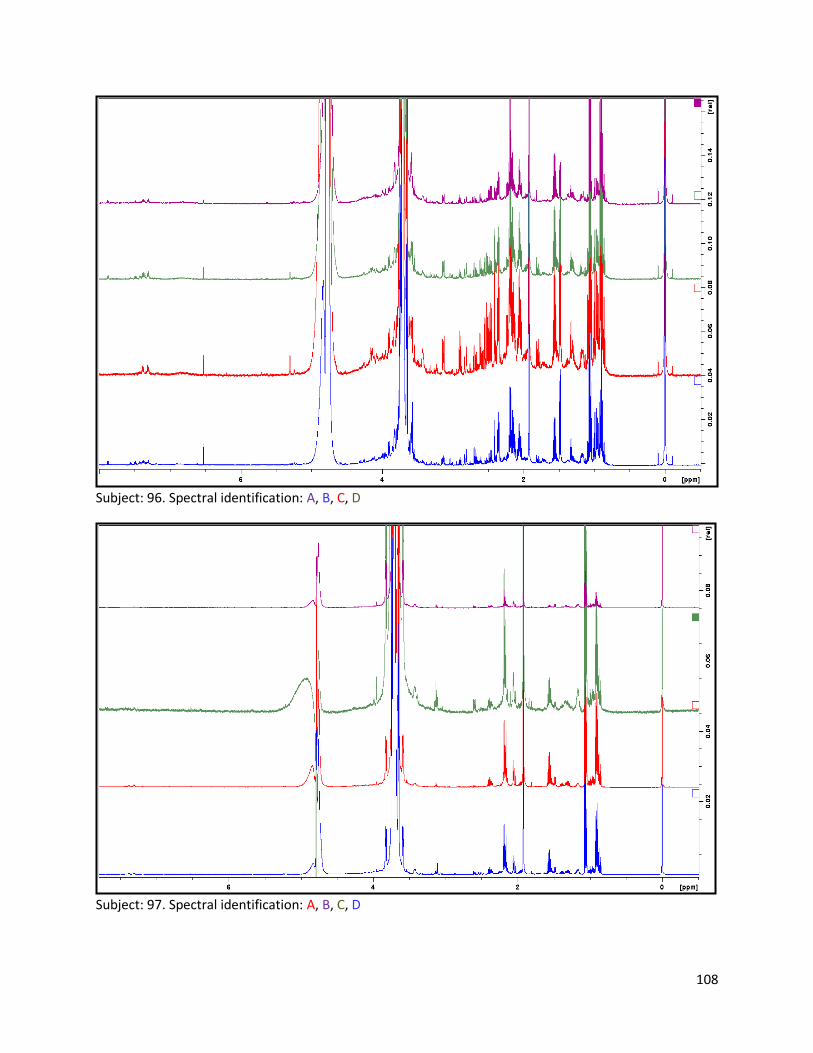
108
Subject: 96. Spectral identification: A, B, C, D
Subject: 97. Spectral identification: A, B, C, D
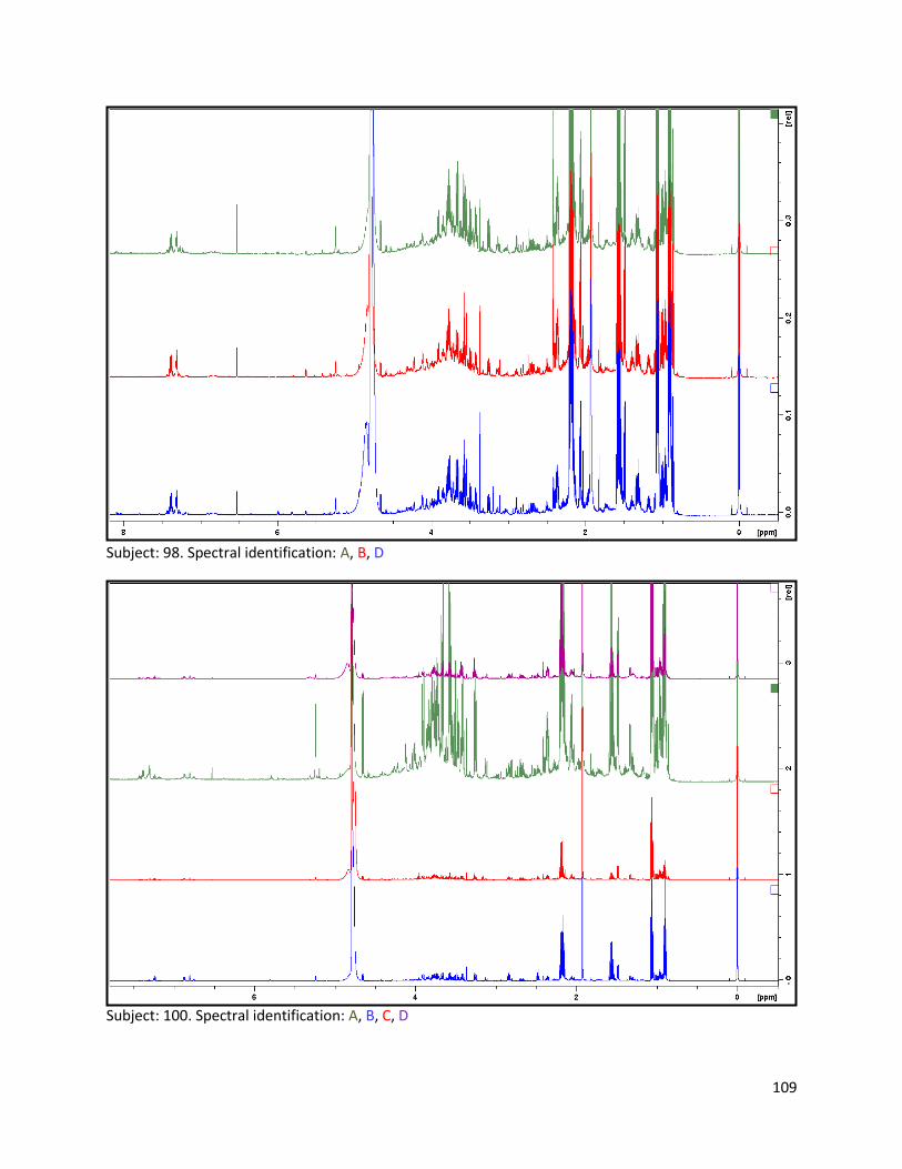
109
Subject: 98. Spectral identification: A, B, D
Subject: 100. Spectral identification: A, B, C, D
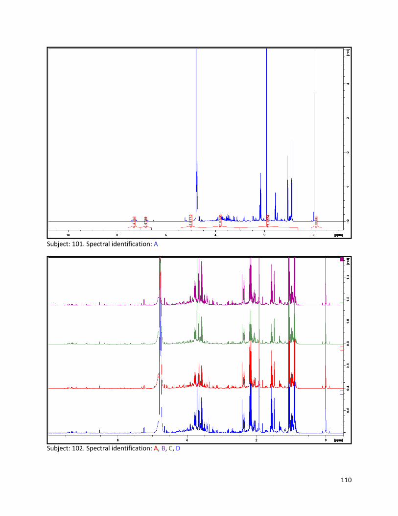
110
Subject: 101. Spectral identification: A
Subject: 102. Spectral identification: A, B, C, D
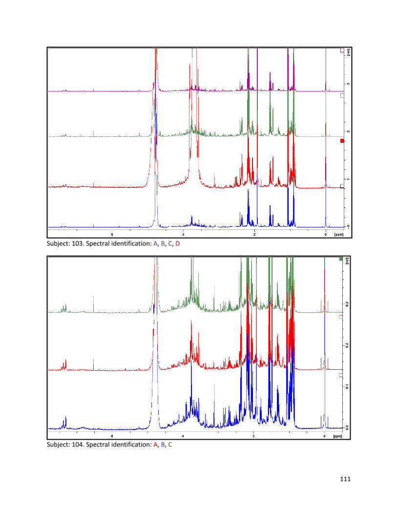
111
Subject: 103. Spectral identification: A, B, C, D
Subject: 104. Spectral identification: A, B, C
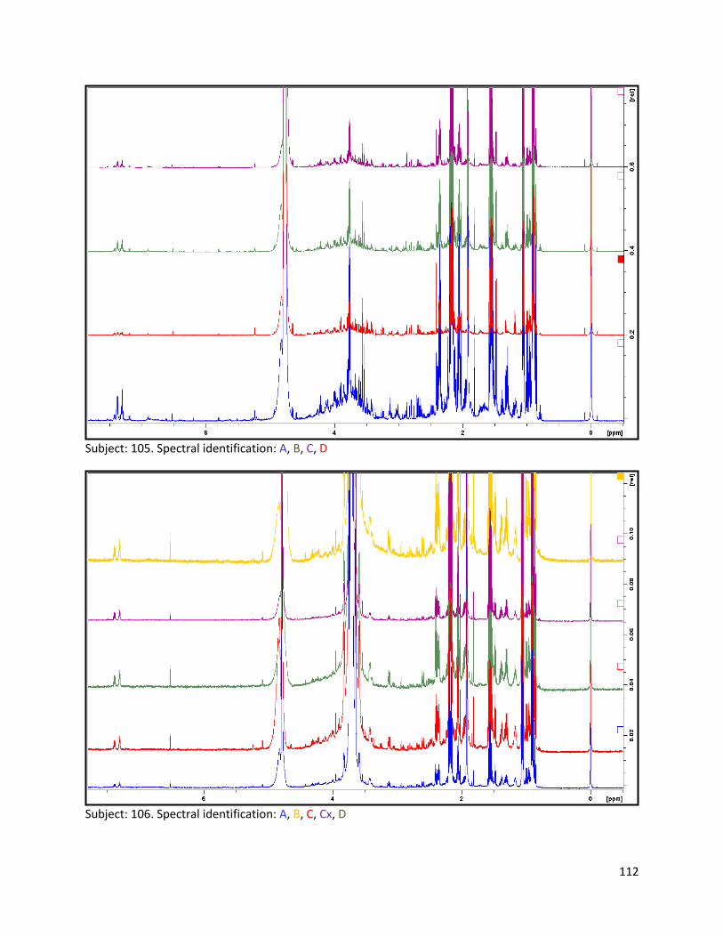
112
Subject: 105. Spectral identification: A, B, C, D
Subject: 106. Spectral identification: A, B, C, Cx, D
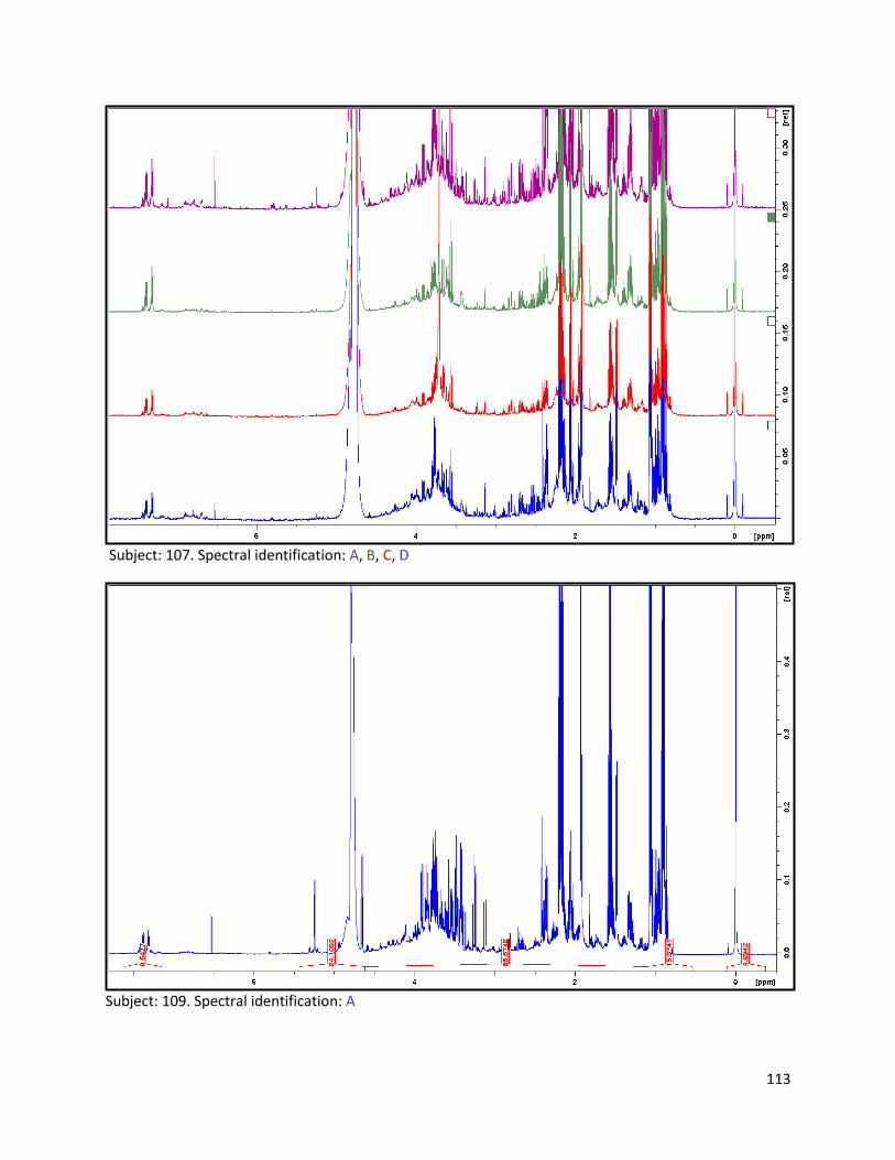
113
Subject: 107. Spectral identification: A, B, C, D
Subject: 109. Spectral identification: A
114
Subject: 117. Spectral identification: A, B, C, D
Subject: 119. Spectral identification: A, B
115
Subject: 120. Spectral identification: A, B, C, D
Subject: 121. Spectral identification: A, C, D
116
Subject: 122. Spectral identification: A, B, C, D
Subject: 125. Spectral identification: A, B, C, D
117
Subject: 128. Spectral identification: A, B, C, D
Subject: 129. Spectral identification: A, B, C, D
118
Subject: 132. Spectral identification: A, B, C
Subject: 133. Spectral identification: A, B, C, D
119
Subject: 134. Spectral identification: A, B, C, D
Subject: 135. Spectral identification: A, B, C, D
120
Subject: 136. Spectral identification: A, B, C, D
Subject: 138. Spectral identification: A, C
121
Subject: 139. Spectral identification: A, B, C, D
Subject: 140. Spectral identification: B, C
122
Subject: 141. Spectral identification: A, B, C, D
Subject: 142. Spectral identification: A, B, D
123
Subject: 143. Spectral identification: A, B, C, D
Subject: 144. Spectral identification: A, B, C, D
124
Subject: 145. Spectral identification: A, B, C, D
Subject: 147. Spectral identification: A, B, C, D
125
Subject: 148. Spectral identification: A, B, C, D
Subject: 150. Spectral identification: A, B, C, D
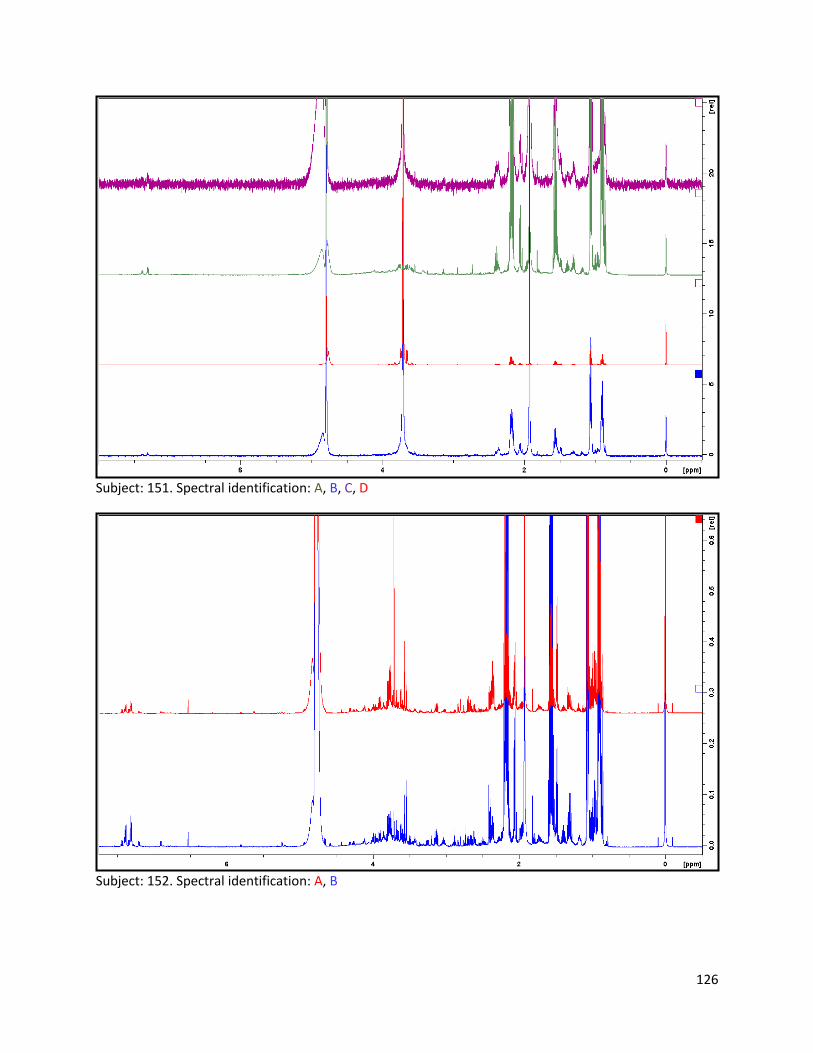
126
Subject: 151. Spectral identification: A, B, C, D
Subject: 152. Spectral identification: A, B
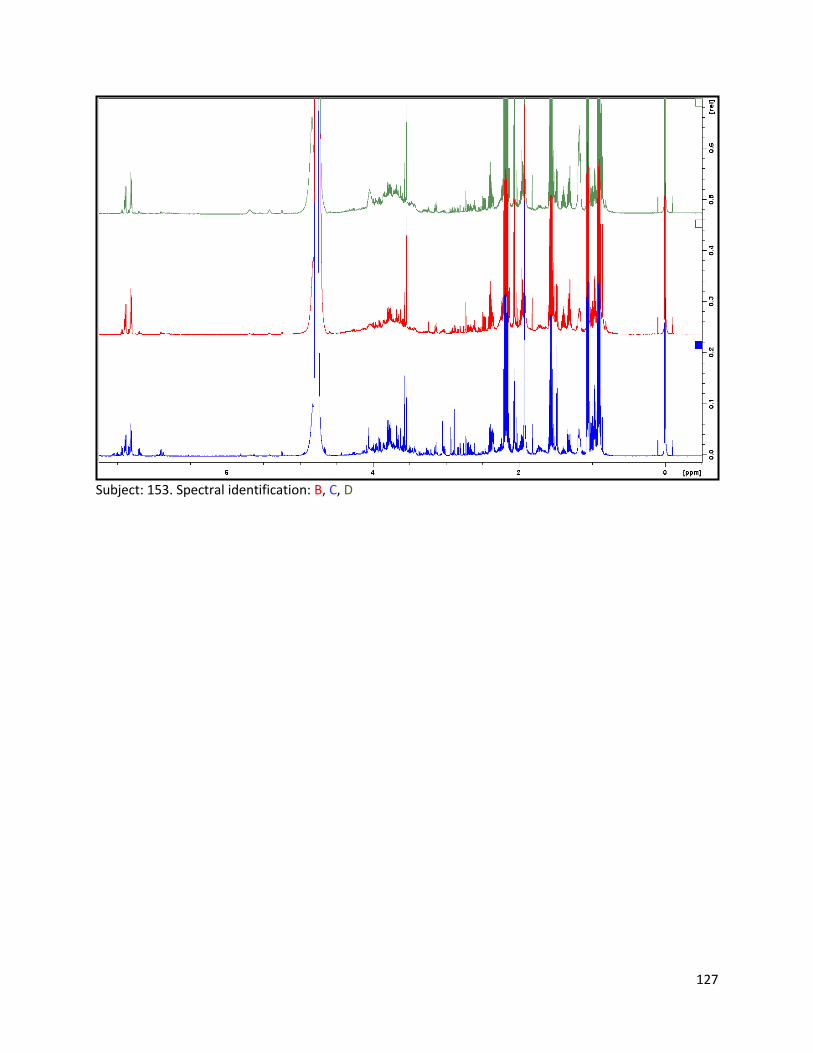
127
Subject: 153. Spectral identification: B, C, D
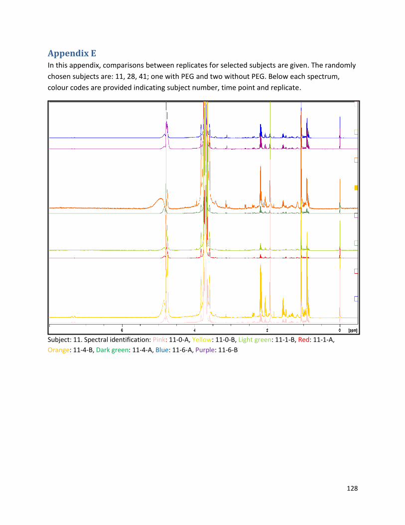
128
Appendix E In this appendix, comparisons between replicates for selected subjects are given. The randomly
chosen subjects are: 11, 28, 41; one with PEG and two without PEG. Below each spectrum,
colour codes are provided indicating subject number, time point and replicate.
Subject: 11. Spectral identification: Pink: 11-0-A, Yellow: 11-0-B, Light green: 11-1-B, Red: 11-1-A,
Orange: 11-4-B, Dark green: 11-4-A, Blue: 11-6-A, Purple: 11-6-B
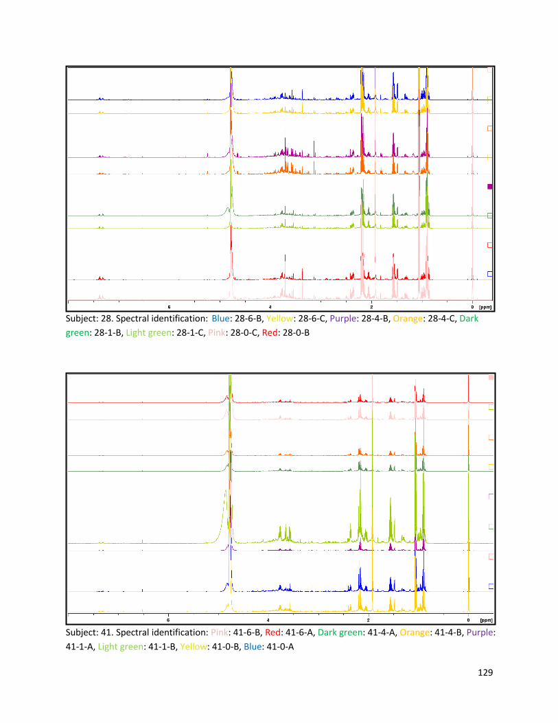
129
Subject: 28. Spectral identification: Blue: 28-6-B, Yellow: 28-6-C, Purple: 28-4-B, Orange: 28-4-C, Dark
green: 28-1-B, Light green: 28-1-C, Pink: 28-0-C, Red: 28-0-B
Subject: 41. Spectral identification: Pink: 41-6-B, Red: 41-6-A, Dark green: 41-4-A, Orange: 41-4-B, Purple:
41-1-A, Light green: 41-1-B, Yellow: 41-0-B, Blue: 41-0-A
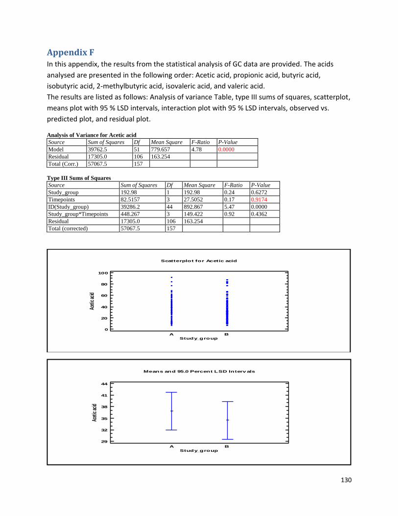
130
Appendix F In this appendix, the results from the statistical analysis of GC data are provided. The acids
analysed are presented in the following order: Acetic acid, propionic acid, butyric acid,
isobutyric acid, 2-methylbutyric acid, isovaleric acid, and valeric acid.
The results are listed as follows: Analysis of variance Table, type III sums of squares, scatterplot,
means plot with 95 % LSD intervals, interaction plot with 95 % LSD intervals, observed vs.
predicted plot, and residual plot.
Analysis of Variance for Acetic acid
Source Sum of Squares Df Mean Square F-Ratio P-Value
Model 39762.5 51 779.657 4.78 0.0000
Residual 17305.0 106 163.254
Total (Corr.) 57067.5 157
Type III Sums of Squares
Source Sum of Squares Df Mean Square F-Ratio P-Value
Study_group 192.98 1 192.98 0.24 0.6272
Timepoints 82.5157 3 27.5052 0.17 0.9174
ID(Study_group) 39286.2 44 892.867 5.47 0.0000
Study_group*Timepoints 448.267 3 149.422 0.92 0.4362
Residual 17305.0 106 163.254
Total (corrected) 57067.5 157
A B
Study_group
Scatterplot for Acetic acid
0
20
40
60
80
100
Acet
ic ac
id
A B
Means and 95.0 Percent LSD Interv als
Study_group
29
32
35
38
41
44
Acet
ic ac
id
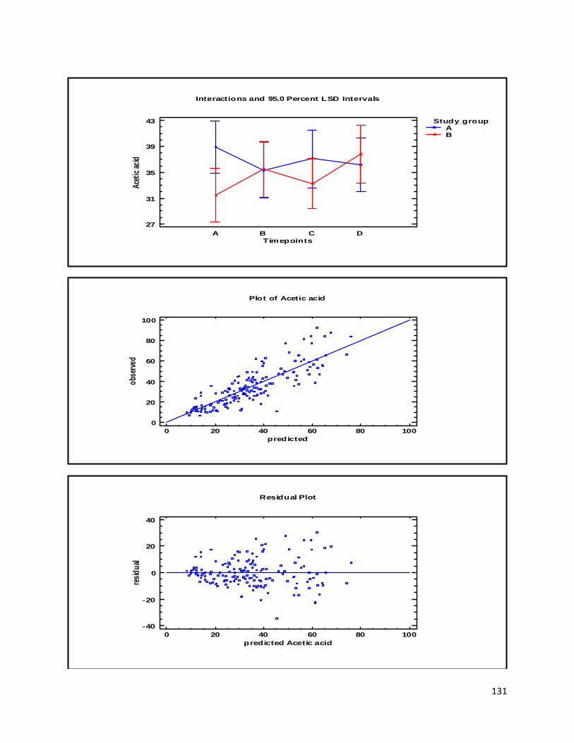
131
Interactions and 95.0 Percent LSD Intervals
Timepoints
27
31
35
39
43
Ace
tic
acid
A B C D
Study_groupAB
Plot of Acetic acid
0 20 40 60 80 100
predicted
0
20
40
60
80
100
obs
erve
d
0 20 40 60 80 100
predicted Acetic acid
Residual Plot
-40
-20
0
20
40
resi
du
al
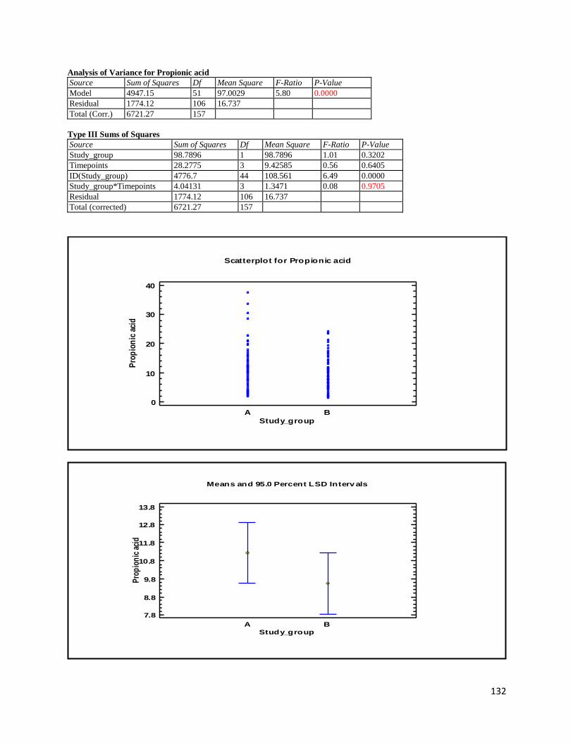
132
Analysis of Variance for Propionic acid
Source Sum of Squares Df Mean Square F-Ratio P-Value
Model 4947.15 51 97.0029 5.80 0.0000
Residual 1774.12 106 16.737
Total (Corr.) 6721.27 157
Type III Sums of Squares
Source Sum of Squares Df Mean Square F-Ratio P-Value
Study_group 98.7896 1 98.7896 1.01 0.3202
Timepoints 28.2775 3 9.42585 0.56 0.6405
ID(Study_group) 4776.7 44 108.561 6.49 0.0000
Study_group*Timepoints 4.04131 3 1.3471 0.08 0.9705
Residual 1774.12 106 16.737
Total (corrected) 6721.27 157
A B
Study_group
Scatterplot for Propionic acid
0
10
20
30
40
Pro
pio
nic
aci
d
A B
Means and 95.0 Percent LSD Interv als
Study_group
7.8
8.8
9.8
10.8
11.8
12.8
13.8
Pro
pio
nic
aci
d
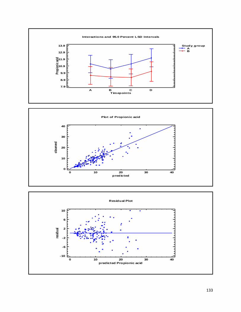
133
Interactions and 95.0 Percent LSD Intervals
Timepoints
7.9
8.9
9.9
10.9
11.9
12.9
13.9
Pro
pio
nic
aci
d
A B C D
Study_groupAB
Plot of Propionic acid
0 10 20 30 40
predicted
0
10
20
30
40
obs
erve
d
0 10 20 30 40
predicted Propionic acid
Residual Plot
-10
-6
-2
2
6
10
resi
du
al
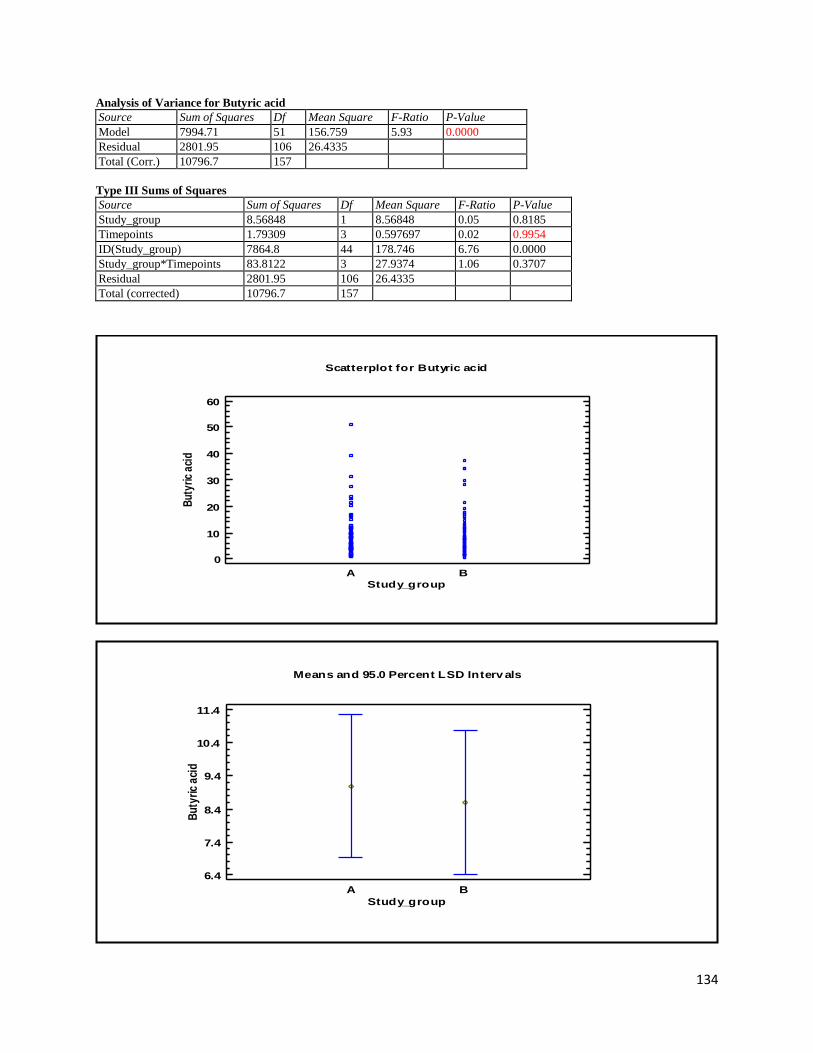
134
Analysis of Variance for Butyric acid
Source Sum of Squares Df Mean Square F-Ratio P-Value
Model 7994.71 51 156.759 5.93 0.0000
Residual 2801.95 106 26.4335
Total (Corr.) 10796.7 157
Type III Sums of Squares
Source Sum of Squares Df Mean Square F-Ratio P-Value
Study_group 8.56848 1 8.56848 0.05 0.8185
Timepoints 1.79309 3 0.597697 0.02 0.9954
ID(Study_group) 7864.8 44 178.746 6.76 0.0000
Study_group*Timepoints 83.8122 3 27.9374 1.06 0.3707
Residual 2801.95 106 26.4335
Total (corrected) 10796.7 157
A B
Study_group
Scatterplot for Butyric acid
0
10
20
30
40
50
60
But
yric
aci
d
A B
Means and 95.0 Percent LSD Interv als
Study_group
6.4
7.4
8.4
9.4
10.4
11.4
Bu
tyri
c a
cid
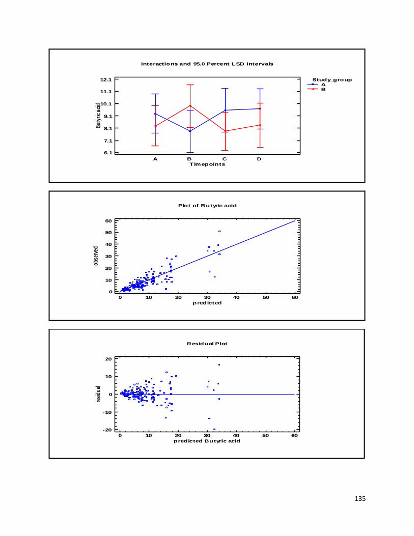
135
Interactions and 95.0 Percent LSD Intervals
Timepoints
6.1
7.1
8.1
9.1
10.1
11.1
12.1
But
yric
aci
d
A B C D
Study_groupAB
Plot of Butyric acid
0 10 20 30 40 50 60
predicted
0
10
20
30
40
50
60
obs
erve
d
0 10 20 30 40 50 60
predicted Butyric acid
Residual Plot
-20
-10
0
10
20
resi
du
al
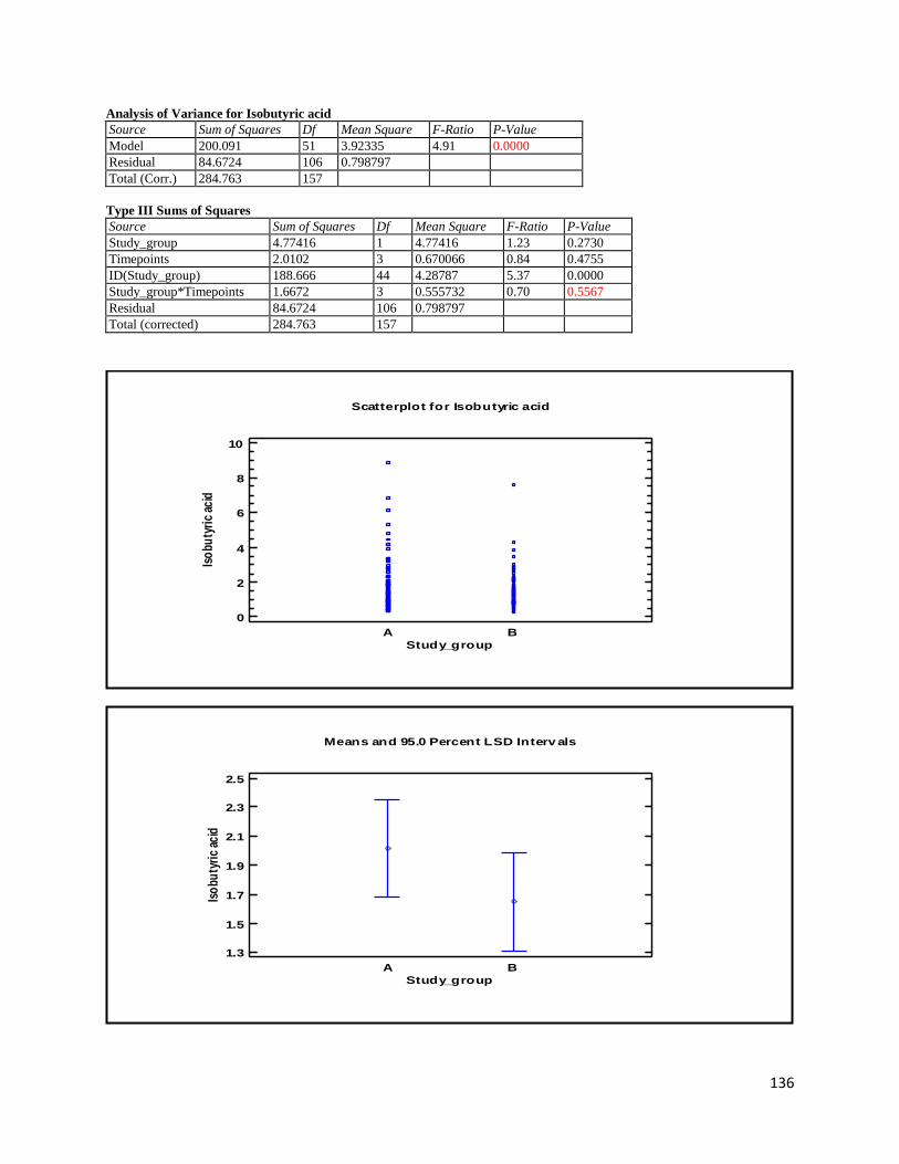
136
Analysis of Variance for Isobutyric acid
Source Sum of Squares Df Mean Square F-Ratio P-Value
Model 200.091 51 3.92335 4.91 0.0000
Residual 84.6724 106 0.798797
Total (Corr.) 284.763 157
Type III Sums of Squares
Source Sum of Squares Df Mean Square F-Ratio P-Value
Study_group 4.77416 1 4.77416 1.23 0.2730
Timepoints 2.0102 3 0.670066 0.84 0.4755
ID(Study_group) 188.666 44 4.28787 5.37 0.0000
Study_group*Timepoints 1.6672 3 0.555732 0.70 0.5567
Residual 84.6724 106 0.798797
Total (corrected) 284.763 157
A B
Study_group
Scatterplot for Isobutyric acid
0
2
4
6
8
10
Iso
buty
ric
acid
A B
Means and 95.0 Percent LSD Interv als
Study_group
1.3
1.5
1.7
1.9
2.1
2.3
2.5
Iso
buty
ric
acid
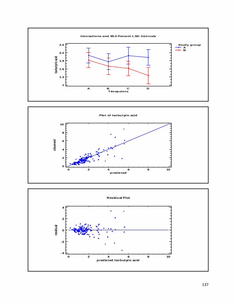
137
Interactions and 95.0 Percent LSD Intervals
Timepoints
1
1.3
1.6
1.9
2.2
2.5
Iso
buty
ric
acid
A B C D
Study_groupAB
Plot of Isobutyric acid
0 2 4 6 8 10
predicted
0
2
4
6
8
10
obs
erve
d
0 2 4 6 8 10
predicted Isobutyric acid
Residual Plot
-4
-2
0
2
4
resi
du
al
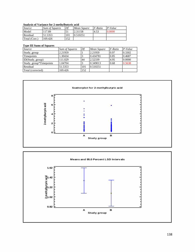
138
Analysis of Variance for 2-methylbutyric acid
Source Sum of Squares Df Mean Square F-Ratio P-Value
Model 117.89 51 2.31158 4.53 0.0000
Residual 51.5353 101 0.510251
Total (Corr.) 169.426 152
Type III Sums of Squares
Source Sum of Squares Df Mean Square F-Ratio P-Value
Study_group 2.21959 1 2.21959 0.97 0.3302
Timepoints 1.30434 3 0.434781 0.85 0.4687
ID(Study_group) 111.029 44 2.52339 4.95 0.0000
Study_group*Timepoints 1.04704 3 0.349013 0.68 0.5638
Residual 51.5353 101 0.510251
Total (corrected) 169.426 152
A B
Study_group
Scatterplot for 2-methylbutyric acid
0
2
4
6
8
2-m
eth
ylbu
tyri
c ac
id
A B
Means and 95.0 Percent LSD Interv als
Study_group
0.82
1.02
1.22
1.42
1.62
2-m
eth
ylb
uty
ric
acid
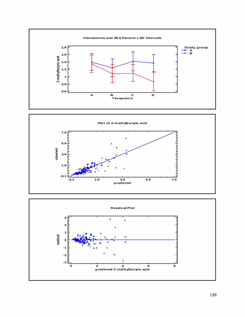
139
Interactions and 95.0 Percent LSD Intervals
Timepoints
0.6
0.8
1
1.2
1.4
1.6
1.8
2-m
eth
ylbu
tyri
c ac
id
A B C D
Study_groupAB
Plot of 2-methylbutyric acid
-0.1 1.9 3.9 5.9 7.9
predicted
-0.1
1.9
3.9
5.9
7.9
obs
erve
d
0 2 4 6 8
predicted 2-methylbutyric acid
Residual Plot
-3
-2
-1
0
1
2
3
resi
du
al
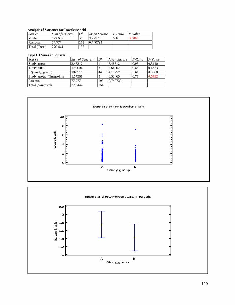
140
Analysis of Variance for Isovaleric acid
Source Sum of Squares Df Mean Square F-Ratio P-Value
Model 192.667 51 3.77778 5.10 0.0000
Residual 77.777 105 0.740733
Total (Corr.) 270.444 156
Type III Sums of Squares
Source Sum of Squares Df Mean Square F-Ratio P-Value
Study_group 3.48312 1 3.48312 0.93 0.3410
Timepoints 1.92006 3 0.64002 0.86 0.4623
ID(Study_group) 182.711 44 4.15252 5.61 0.0000
Study_group*Timepoints 1.57389 3 0.52463 0.71 0.5492
Residual 77.777 105 0.740733
Total (corrected) 270.444 156
A B
Study_group
Scatterplot for Isov aleric acid
0
2
4
6
8
10
Iso
vale
ric
acid
A B
Means and 95.0 Percent LSD Interv als
Study_group
1
1.2
1.4
1.6
1.8
2
2.2
Iso
vale
ric
acid
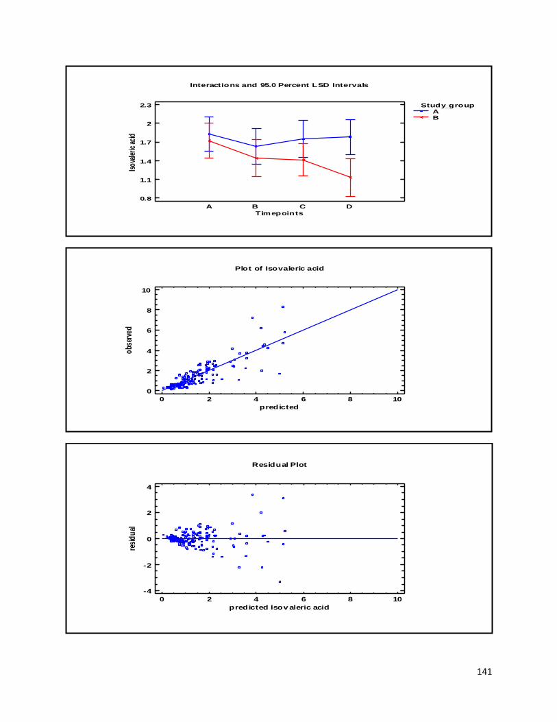
141
Interactions and 95.0 Percent LSD Intervals
Timepoints
0.8
1.1
1.4
1.7
2
2.3
Isov
aler
ic a
cid
A B C D
Study_groupAB
Plot of Isovaleric acid
0 2 4 6 8 10
predicted
0
2
4
6
8
10
obs
erve
d
0 2 4 6 8 10
predicted Isov aleric acid
Residual Plot
-4
-2
0
2
4
resi
du
al
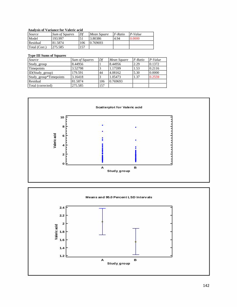
142
Analysis of Variance for Valeric acid
Source Sum of Squares Df Mean Square F-Ratio P-Value
Model 193.997 51 3.80386 4.94 0.0000
Residual 81.5874 106 0.769693
Total (Corr.) 275.585 157
Type III Sums of Squares
Source Sum of Squares Df Mean Square F-Ratio P-Value
Study_group 8.44956 1 8.44956 2.29 0.1372
Timepoints 3.52798 3 1.17599 1.53 0.2116
ID(Study_group) 179.591 44 4.08162 5.30 0.0000
Study_group*Timepoints 3.16418 3 1.05473 1.37 0.2559
Residual 81.5874 106 0.769693
Total (corrected) 275.585 157
A B
Study_group
Scatterplot for Valeric acid
0
2
4
6
8
10
Val
eric
aci
d
A B
Means and 95.0 Percent LSD Interv als
Study_group
1.2
1.4
1.6
1.8
2
2.2
2.4
Val
eric
aci
d
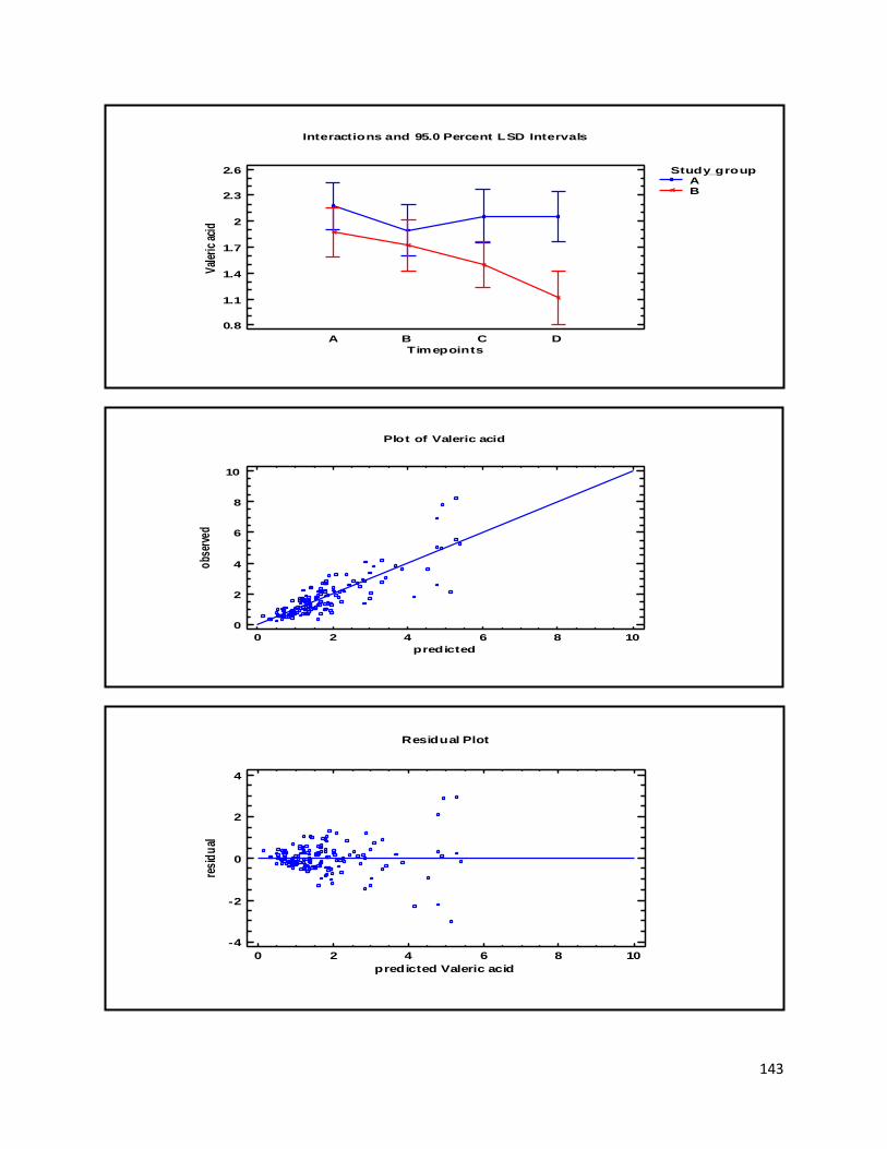
143
Interactions and 95.0 Percent LSD Intervals
Timepoints
0.8
1.1
1.4
1.7
2
2.3
2.6
Val
eric
aci
d
A B C D
Study_groupAB
Plot of Valeric acid
0 2 4 6 8 10
predicted
0
2
4
6
8
10
obs
erve
d
0 2 4 6 8 10
predicted Valeric acid
Residual Plot
-4
-2
0
2
4
resi
du
al
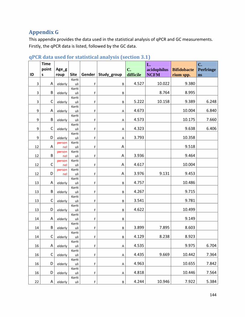
144
Appendix G This appendix provides the data used in the statistical analysis of qPCR and GC measurements.
Firstly, the qPCR data is listed, followed by the GC data.
qPCR data used for statistical analysis (section 3.1)
ID
Timepoints
Age_group Site Gender Study_group
C.
difficile
L.
acidophilus
NCFM
Bifidobacte
rium spp.
C.
Perfringe
ns
3 A elderly Kertt
uli F B 4.527 10.022 9.380
3 B elderly Kertt
uli F B 8.764 8.995
3 C elderly Kertt
uli F B 5.222 10.158 9.389 6.248
9 A elderly Kertt
uli F A 4.673 10.004 6.840
9 B elderly Kertt
uli F A 4.573 10.175 7.660
9 C elderly Kertt
uli F A 4.323 9.638 6.406
9 D elderly Kertt
uli F A 3.793 10.358
12 A person
nel Kertt
uli F A 9.518
12 B person
nel Kertt
uli F A 3.936 9.464
12 C person
nel Kertt
uli F A 4.617 10.004
12 D person
nel Kertt
uli F A 3.976 9.131 9.453
13 A elderly Kertt
uli F B 4.757 10.486
13 B elderly Kertt
uli F B 4.267 9.715
13 C elderly Kertt
uli F B 3.541 9.781
13 D elderly Kertt
uli F B 4.622 10.499
14 A elderly Kertt
uli F B 9.149
14 B elderly Kertt
uli F B 3.899 7.895 8.603
14 C elderly Kertt
uli F B 4.129 8.238 8.923
16 A elderly Kertt
uli F A 4.535 9.975 6.704
16 C elderly Kertt
uli F A 4.435 9.669 10.442 7.364
16 D elderly Kertt
uli F A 4.963 10.655 7.842
16 D elderly Kertt
uli F A 4.818 10.446 7.564
22 A elderly Kertt
uli F B 4.244 10.946 7.922 5.384
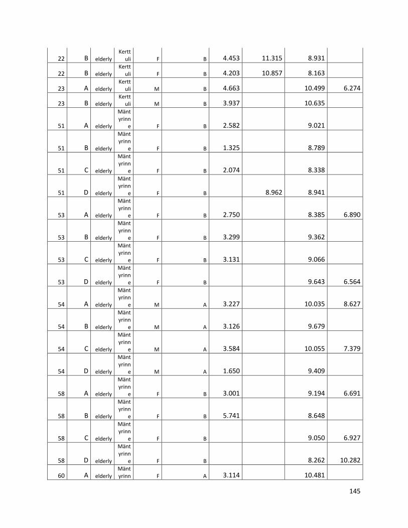
145
22 B elderly Kertt
uli F B 4.453 11.315 8.931
22 B elderly Kertt
uli F B 4.203 10.857 8.163
23 A elderly Kertt
uli M B 4.663 10.499 6.274
23 B elderly Kertt
uli M B 3.937 10.635
51 A elderly
Mäntyrinn
e F B 2.582 9.021
51 B elderly
Mäntyrinn
e F B 1.325 8.789
51 C elderly
Mäntyrinn
e F B 2.074 8.338
51 D elderly
Mäntyrinn
e F B 8.962 8.941
53 A elderly
Mäntyrinn
e F B 2.750 8.385 6.890
53 B elderly
Mäntyrinn
e F B 3.299 9.362
53 C elderly
Mäntyrinn
e F B 3.131 9.066
53 D elderly
Mäntyrinn
e F B 9.643 6.564
54 A elderly
Mäntyrinn
e M A 3.227 10.035 8.627
54 B elderly
Mäntyrinn
e M A 3.126 9.679
54 C elderly
Mäntyrinn
e M A 3.584 10.055 7.379
54 D elderly
Mäntyrinn
e M A 1.650 9.409
58 A elderly
Mäntyrinn
e F B 3.001 9.194 6.691
58 B elderly
Mäntyrinn
e F B 5.741 8.648
58 C elderly
Mäntyrinn
e F B 9.050 6.927
58 D elderly
Mäntyrinn
e F B 8.262 10.282
60 A elderly Mäntyrinn F A 3.114 10.481
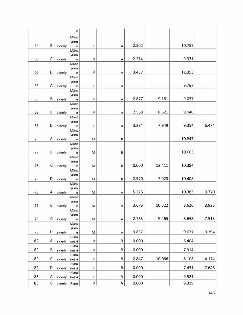
146
e
60 B elderly
Mäntyrinn
e F A 2.502 10.757
60 C elderly
Mäntyrinn
e F A 2.214 9.931
60 D elderly
Mäntyrinn
e F A 3.457 11.353
63 A elderly
Mäntyrinn
e F A 9.767
63 B elderly
Mäntyrinn
e F A 2.877 9.161 9.037
63 C elderly
Mäntyrinn
e F A 2.568 8.521 9.040
63 D elderly
Mäntyrinn
e F A 3.284 7.949 9.354 6.474
73 A elderly
Mäntyrinn
e M B 10.847
73 B elderly
Mäntyrinn
e M B 10.603
73 C elderly
Mäntyrinn
e M B 0.000 12.411 10.384
73 D elderly
Mäntyrinn
e M B 2.570 7.923 10.408
75 A elderly
Mäntyrinn
e M A 5.226 10.383 9.770
75 B elderly
Mäntyrinn
e M A 3.676 10.522 8.620 8.825
75 C elderly
Mäntyrinn
e M A 2.763 9.465 8.658 7.513
75 D elderly
Mäntyrinn
e M A 3.837 9.637 9.394
82 A elderly Runo
smäki F B 0.000 6.404
82 B elderly Runo
smäki F B 0.000 7.314
82 C elderly Runo
smäki F B 2.847 10.066 8.108 4.174
82 D elderly Runo
smäki F B 0.000 7.431 7.646
83 A elderly Runo
smäki F A 0.000 9.521
83 B elderly Runo F A 0.000 9.319
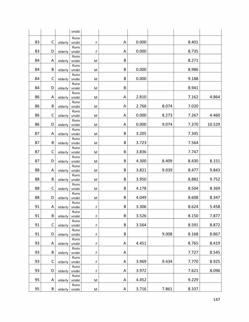
147
smäki
83 C elderly Runo
smäki F A 0.000 8.401
83 D elderly Runo
smäki F A 0.000 8.735
84 A elderly Runo
smäki M B 8.271
84 B elderly Runo
smäki M B 0.000 8.986
84 C elderly Runo
smäki M B 0.000 9.188
84 D elderly Runo
smäki M B 8.941
86 A elderly Runo
smäki M A 2.810 7.162 4.864
86 B elderly Runo
smäki M A 2.766 8.074 7.020
86 C elderly Runo
smäki M A 0.000 8.273 7.267 4.460
86 D elderly Runo
smäki M A 0.000 9.074 7.370 10.529
87 A elderly Runo
smäki M B 3.205 7.345
87 B elderly Runo
smäki M B 3.723 7.564
87 C elderly Runo
smäki M B 3.836 7.747
87 D elderly Runo
smäki M B 4.300 8.409 8.430 8.151
88 A elderly Runo
smäki M B 3.821 9.039 8.477 9.843
88 B elderly Runo
smäki M B 3.950 8.882 9.752
88 C elderly Runo
smäki M B 4.178 8.504 8.369
88 D elderly Runo
smäki M B 4.049 8.608 8.347
91 A elderly Runo
smäki F B 3.306 8.624 5.458
91 B elderly Runo
smäki F B 3.526 8.150 7.877
91 C elderly Runo
smäki F B 3.564 8.591 8.872
91 D elderly Runo
smäki F B 9.008 8.168 8.867
93 A elderly Runo
smäki F A 4.451 8.765 8.419
93 B elderly Runo
smäki F A 7.727 8.545
93 C elderly Runo
smäki F A 3.969 9.434 7.770 8.925
93 D elderly Runo
smäki F A 3.972 7.621 8.096
95 A elderly Runo
smäki M A 4.452 9.229
95 B elderly Runo
smäki M A 3.716 7.861 8.337
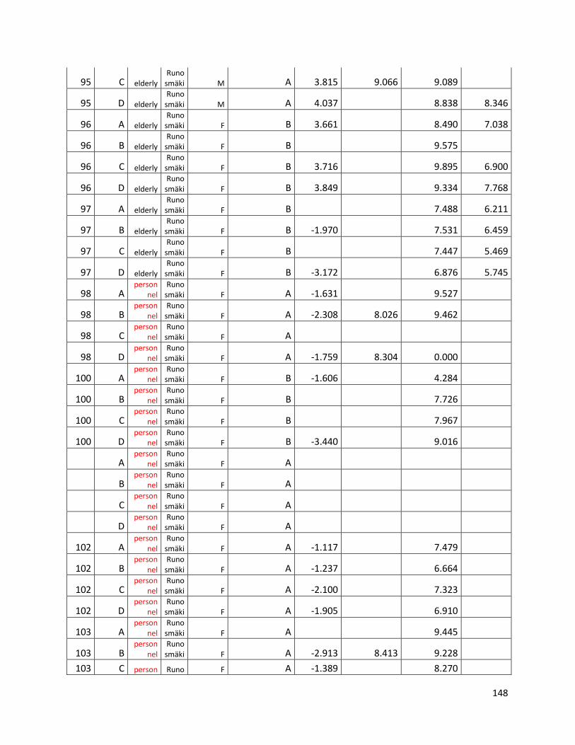
148
95 C elderly Runo
smäki M A 3.815 9.066 9.089
95 D elderly Runo
smäki M A 4.037 8.838 8.346
96 A elderly Runo
smäki F B 3.661 8.490 7.038
96 B elderly Runo
smäki F B 9.575
96 C elderly Runo
smäki F B 3.716 9.895 6.900
96 D elderly Runo
smäki F B 3.849 9.334 7.768
97 A elderly Runo
smäki F B 7.488 6.211
97 B elderly Runo
smäki F B -1.970 7.531 6.459
97 C elderly Runo
smäki F B 7.447 5.469
97 D elderly Runo
smäki F B -3.172 6.876 5.745
98 A person
nel Runo
smäki F A -1.631 9.527
98 B person
nel Runo
smäki F A -2.308 8.026 9.462
98 C person
nel Runo
smäki F A
98 D person
nel Runo
smäki F A -1.759 8.304 0.000
100 A person
nel Runo
smäki F B -1.606 4.284
100 B person
nel Runo
smäki F B 7.726
100 C person
nel Runo
smäki F B 7.967
100 D person
nel Runo
smäki F B -3.440 9.016
A person
nel Runo
smäki F A
B person
nel Runo
smäki F A
C person
nel Runo
smäki F A
D person
nel Runo
smäki F A
102 A person
nel Runo
smäki F A -1.117 7.479
102 B person
nel Runo
smäki F A -1.237 6.664
102 C person
nel Runo
smäki F A -2.100 7.323
102 D person
nel Runo
smäki F A -1.905 6.910
103 A person
nel Runo
smäki F A 9.445
103 B person
nel Runo
smäki F A -2.913 8.413 9.228
103 C person Runo F A -1.389 8.270
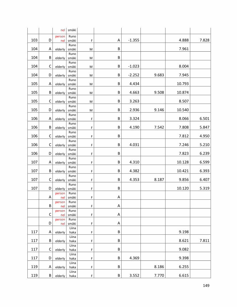
149
nel smäki
103 D person
nel Runo
smäki F A -1.355 4.888 7.828
104 A elderly Runo
smäki M B 7.961
104 B elderly Runo
smäki M B
104 C elderly Runo
smäki M B -1.023 8.004
104 D elderly Runo
smäki M B -2.252 9.683 7.945
105 A elderly Runo
smäki M B 4.434 10.793
105 B elderly Runo
smäki M B 4.663 9.508 10.874
105 C elderly Runo
smäki M B 3.263 8.507
105 D elderly Runo
smäki M B 2.936 9.146 10.540
106 A elderly Runo
smäki F B 3.324 8.066 6.501
106 B elderly Runo
smäki F B 4.190 7.542 7.808 5.847
106 C elderly Runo
smäki F B 7.812 4.950
106 C elderly Runo
smäki F B 4.031 7.246 5.210
106 D elderly Runo
smäki F B 7.823 6.239
107 A elderly Runo
smäki F B 4.310 10.128 6.599
107 B elderly Runo
smäki F B 4.382 10.421 6.393
107 C elderly Runo
smäki F B 4.353 8.187 9.856 6.407
107 D elderly Runo
smäki F B 10.120 5.319
A person
nel Runo
smäki F A
B person
nel Runo
smäki F A
C person
nel Runo
smäki F A
D person
nel Runo
smäki F A
117 A elderly Liinahaka F B 9.198
117 B elderly Liinahaka F B 8.621 7.811
117 C elderly Liinahaka F B 9.082
117 D elderly Liinahaka F B 4.369 9.398
119 A elderly Liinahaka F B 8.186 6.255
119 B elderly Liinahaka F B 3.552 7.770 6.615
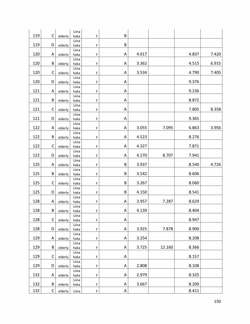
150
119 C elderly Liinahaka F B
119 D elderly Liinahaka F B
120 A elderly Liinahaka F A 4.017 4.837 7.420
120 B elderly Liinahaka F A 3.362 4.515 6.915
120 C elderly Liinahaka F A 3.534 4.790 7.405
120 D elderly Liinahaka F A 9.376
121 A elderly Liinahaka F A 9.236
121 B elderly Liinahaka F A 8.872
121 C elderly Liinahaka F A 7.805 8.358
121 D elderly Liinahaka F A 9.365
122 A elderly Liinahaka F A 3.055 7.095 6.863 3.956
122 B elderly Liinahaka F A 4.523 8.276
122 C elderly Liinahaka F A 4.327 7.871
122 D elderly Liinahaka F A 4.270 8.707 7.941
125 A elderly Liinahaka F B 3.937 8.540 4.726
125 B elderly Liinahaka F B 3.542 8.606
125 C elderly Liinahaka F B 3.267 8.060
125 D elderly Liinahaka F B 4.150 8.541
128 A elderly Liinahaka F A 3.957 7.287 8.629
128 B elderly Liinahaka F A 4.139 8.404
128 C elderly Liinahaka F A 8.947
128 D elderly Liinahaka F A 3.925 7.878 8.900
129 A elderly Liinahaka F A 3.254 8.208
129 B elderly Liinahaka F A 3.725 12.160 8.366
129 C elderly Liinahaka F A 8.157
129 D elderly Liinahaka F A 2.808 8.108
132 A elderly Liinahaka F A 2.979 8.325
132 B elderly Liinahaka F A 3.667 8.200
132 C elderly Liina F A 8.411

151
haka
132 D elderly Liinahaka F A 3.992 8.404
133 A elderly Liinahaka F A 0.000 10.150 8.324 4.341
133 B elderly Liinahaka F A 0.000 9.576 8.511 6.249
133 C elderly Liinahaka F A 0.000 8.443 8.243 4.866
133 D elderly Liinahaka F A 9.616 8.629 5.740
134 A elderly Liinahaka F A 0.000 8.195
134 B elderly Liinahaka F A 2.701 8.067
134 C elderly Liinahaka F A 0.000 7.450 8.977
134 D elderly Liinahaka F A 3.435 8.177 8.422
135 A elderly Liinahaka M B 0.000 8.305
135 B elderly Liinahaka M B 0.000 8.811
135 C elderly Liinahaka M B 3.765 8.910
135 D elderly Liinahaka M B 3.957 9.007
136 A person
nel Liinahaka F B 0.000 8.708 8.764
136 B person
nel Liinahaka F B 0.000 7.723 8.815
136 C person
nel Liinahaka F B 4.097 8.913
136 D person
nel Liinahaka F B 8.507 9.200
138 A elderly Liinahaka F B 0.000 7.410 8.939
138 B elderly Liinahaka F B 3.547 9.086 5.253
138 C elderly Liinahaka F B 0.000 9.466 4.844
138 D elderly Liinahaka F B
139 A elderly Liinahaka F A 3.881 8.840
139 B elderly Liinahaka F A 0.000 7.307 8.688
139 C elderly Liinahaka F A 0.000 7.251 9.018
139 D elderly Liinahaka F A 8.720
140 A elderly Liinahaka M A 4.265 11.003 8.096 4.431
140 B elderly Liinahaka M A 4.293 8.939 8.445 4.175
140 C elderly Liinahaka M A 7.334 8.125
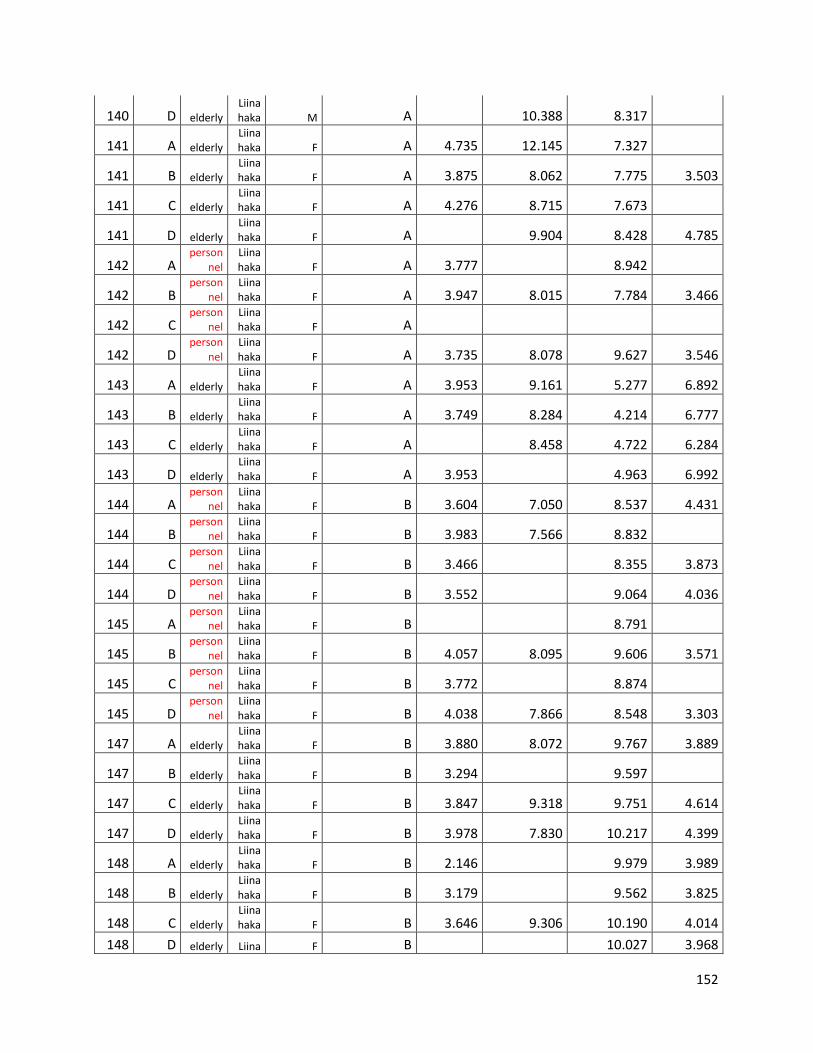
152
140 D elderly Liinahaka M A 10.388 8.317
141 A elderly Liinahaka F A 4.735 12.145 7.327
141 B elderly Liinahaka F A 3.875 8.062 7.775 3.503
141 C elderly Liinahaka F A 4.276 8.715 7.673
141 D elderly Liinahaka F A 9.904 8.428 4.785
142 A person
nel Liinahaka F A 3.777 8.942
142 B person
nel Liinahaka F A 3.947 8.015 7.784 3.466
142 C person
nel Liinahaka F A
142 D person
nel Liinahaka F A 3.735 8.078 9.627 3.546
143 A elderly Liinahaka F A 3.953 9.161 5.277 6.892
143 B elderly Liinahaka F A 3.749 8.284 4.214 6.777
143 C elderly Liinahaka F A 8.458 4.722 6.284
143 D elderly Liinahaka F A 3.953 4.963 6.992
144 A person
nel Liinahaka F B 3.604 7.050 8.537 4.431
144 B person
nel Liinahaka F B 3.983 7.566 8.832
144 C person
nel Liinahaka F B 3.466 8.355 3.873
144 D person
nel Liinahaka F B 3.552 9.064 4.036
145 A person
nel Liinahaka F B 8.791
145 B person
nel Liinahaka F B 4.057 8.095 9.606 3.571
145 C person
nel Liinahaka F B 3.772 8.874
145 D person
nel Liinahaka F B 4.038 7.866 8.548 3.303
147 A elderly Liinahaka F B 3.880 8.072 9.767 3.889
147 B elderly Liinahaka F B 3.294 9.597
147 C elderly Liinahaka F B 3.847 9.318 9.751 4.614
147 D elderly Liinahaka F B 3.978 7.830 10.217 4.399
148 A elderly Liinahaka F B 2.146 9.979 3.989
148 B elderly Liinahaka F B 3.179 9.562 3.825
148 C elderly Liinahaka F B 3.646 9.306 10.190 4.014
148 D elderly Liina F B 10.027 3.968
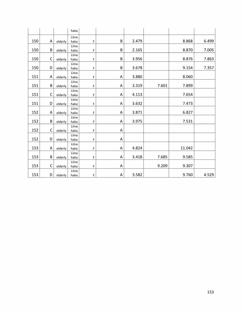
153
haka
150 A elderly Liinahaka F B 2.479 8.868 6.499
150 B elderly Liinahaka F B 2.165 8.870 7.005
150 C elderly Liinahaka F B 3.956 8.876 7.863
150 D elderly Liinahaka F B 3.678 9.154 7.357
151 A elderly Liinahaka F A 3.880 8.060
151 B elderly Liinahaka F A 3.319 7.601 7.899
151 C elderly Liinahaka F A 4.113 7.654
151 D elderly Liinahaka F A 3.632 7.473
152 A elderly Liinahaka F A 3.871 6.827
152 B elderly Liinahaka F A 3.975 7.531
152 C elderly Liinahaka F A
152 D elderly Liinahaka F A
153 A elderly Liinahaka F A 4.824 11.042
153 B elderly Liinahaka F A 3.418 7.685 9.585
153 C elderly Liinahaka F A 9.209 9.307
153 D elderly Liinahaka F A 3.582 9.760 4.529
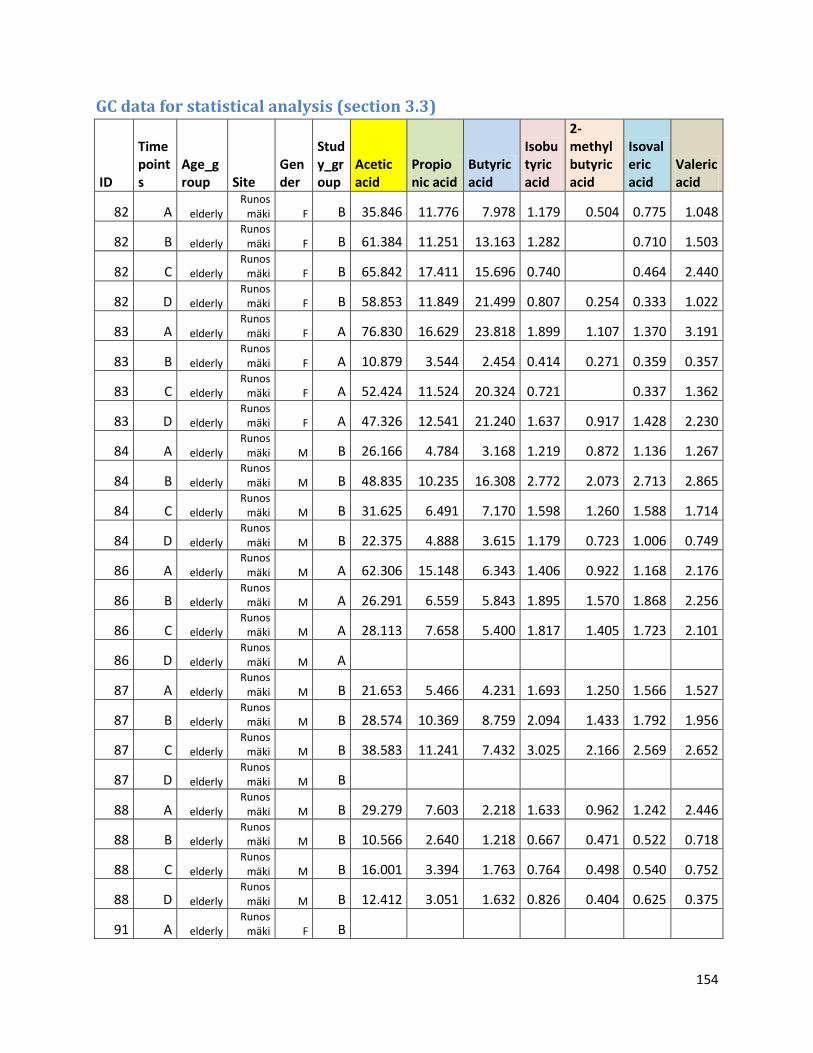
154
GC data for statistical analysis (section 3.3)
ID
Timepoints
Age_group Site
Gender
Study_group
Acetic acid
Propionic acid
Butyric acid
Isobutyric acid
2-methylbutyric acid
Isovaleric acid
Valeric acid
82 A elderly Runos
mäki F B 35.846 11.776 7.978 1.179 0.504 0.775 1.048
82 B elderly Runos
mäki F B 61.384 11.251 13.163 1.282 0.710 1.503
82 C elderly Runos
mäki F B 65.842 17.411 15.696 0.740 0.464 2.440
82 D elderly Runos
mäki F B 58.853 11.849 21.499 0.807 0.254 0.333 1.022
83 A elderly Runos
mäki F A 76.830 16.629 23.818 1.899 1.107 1.370 3.191
83 B elderly Runos
mäki F A 10.879 3.544 2.454 0.414 0.271 0.359 0.357
83 C elderly Runos
mäki F A 52.424 11.524 20.324 0.721 0.337 1.362
83 D elderly Runos
mäki F A 47.326 12.541 21.240 1.637 0.917 1.428 2.230
84 A elderly Runos
mäki M B 26.166 4.784 3.168 1.219 0.872 1.136 1.267
84 B elderly Runos
mäki M B 48.835 10.235 16.308 2.772 2.073 2.713 2.865
84 C elderly Runos
mäki M B 31.625 6.491 7.170 1.598 1.260 1.588 1.714
84 D elderly Runos
mäki M B 22.375 4.888 3.615 1.179 0.723 1.006 0.749
86 A elderly Runos
mäki M A 62.306 15.148 6.343 1.406 0.922 1.168 2.176
86 B elderly Runos
mäki M A 26.291 6.559 5.843 1.895 1.570 1.868 2.256
86 C elderly Runos
mäki M A 28.113 7.658 5.400 1.817 1.405 1.723 2.101
86 D elderly Runos
mäki M A
87 A elderly Runos
mäki M B 21.653 5.466 4.231 1.693 1.250 1.566 1.527
87 B elderly Runos
mäki M B 28.574 10.369 8.759 2.094 1.433 1.792 1.956
87 C elderly Runos
mäki M B 38.583 11.241 7.432 3.025 2.166 2.569 2.652
87 D elderly Runos
mäki M B
88 A elderly Runos
mäki M B 29.279 7.603 2.218 1.633 0.962 1.242 2.446
88 B elderly Runos
mäki M B 10.566 2.640 1.218 0.667 0.471 0.522 0.718
88 C elderly Runos
mäki M B 16.001 3.394 1.763 0.764 0.498 0.540 0.752
88 D elderly Runos
mäki M B 12.412 3.051 1.632 0.826 0.404 0.625 0.375
91 A elderly Runos
mäki F B
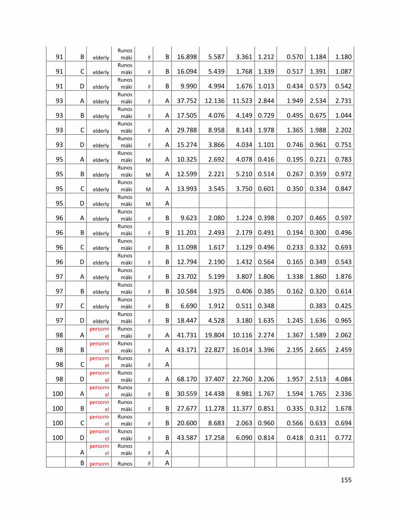
155
91 B elderly Runos
mäki F B 16.898 5.587 3.361 1.212 0.570 1.184 1.180
91 C elderly Runos
mäki F B 16.094 5.439 1.768 1.339 0.517 1.391 1.087
91 D elderly Runos
mäki F B 9.990 4.994 1.676 1.013 0.434 0.573 0.542
93 A elderly Runos
mäki F A 37.752 12.136 11.523 2.844 1.949 2.534 2.731
93 B elderly Runos
mäki F A 17.505 4.076 4.149 0.729 0.495 0.675 1.044
93 C elderly Runos
mäki F A 29.788 8.958 8.143 1.978 1.365 1.988 2.202
93 D elderly Runos
mäki F A 15.274 3.866 4.034 1.101 0.746 0.961 0.751
95 A elderly Runos
mäki M A 10.325 2.692 4.078 0.416 0.195 0.221 0.783
95 B elderly Runos
mäki M A 12.599 2.221 5.210 0.514 0.267 0.359 0.972
95 C elderly Runos
mäki M A 13.993 3.545 3.750 0.601 0.350 0.334 0.847
95 D elderly Runos
mäki M A
96 A elderly Runos
mäki F B 9.623 2.080 1.224 0.398 0.207 0.465 0.597
96 B elderly Runos
mäki F B 11.201 2.493 2.179 0.491 0.194 0.300 0.496
96 C elderly Runos
mäki F B 11.098 1.617 1.129 0.496 0.233 0.332 0.693
96 D elderly Runos
mäki F B 12.794 2.190 1.432 0.564 0.165 0.349 0.543
97 A elderly Runos
mäki F B 23.702 5.199 3.807 1.806 1.338 1.860 1.876
97 B elderly Runos
mäki F B 10.584 1.925 0.406 0.385 0.162 0.320 0.614
97 C elderly Runos
mäki F B 6.690 1.912 0.511 0.348 0.383 0.425
97 D elderly Runos
mäki F B 18.447 4.528 3.180 1.635 1.245 1.636 0.965
98 A personn
el Runos
mäki F A 41.731 19.804 10.116 2.274 1.367 1.589 2.062
98 B personn
el Runos
mäki F A 43.171 22.827 16.014 3.396 2.195 2.665 2.459
98 C personn
el Runos
mäki F A
98 D personn
el Runos
mäki F A 68.170 37.407 22.760 3.206 1.957 2.513 4.084
100 A personn
el Runos
mäki F B 30.559 14.438 8.981 1.767 1.594 1.765 2.336
100 B personn
el Runos
mäki F B 27.677 11.278 11.377 0.851 0.335 0.312 1.678
100 C personn
el Runos
mäki F B 20.600 8.683 2.063 0.960 0.566 0.633 0.694
100 D personn
el Runos
mäki F B 43.587 17.258 6.090 0.814 0.418 0.311 0.772
A personn
el Runos
mäki F A
B personn Runos F A
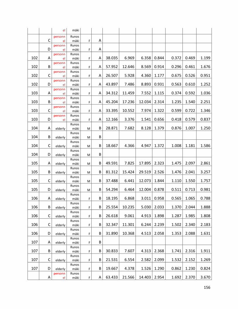
156
el mäki
C personn
el Runos
mäki F A
D personn
el Runos
mäki F A
102 A personn
el Runos
mäki F A 38.035 6.969 6.358 0.844 0.372 0.469 1.199
102 B personn
el Runos
mäki F A 57.952 12.646 8.569 0.914 0.296 0.461 1.676
102 C personn
el Runos
mäki F A 26.507 5.928 4.360 1.177 0.675 0.526 0.951
102 D personn
el Runos
mäki F A 43.897 7.486 8.893 0.931 0.563 0.610 1.252
103 A personn
el Runos
mäki F A 34.312 11.459 7.552 1.115 0.374 0.592 1.036
103 B personn
el Runos
mäki F A 45.204 17.236 12.034 2.314 1.235 1.540 2.251
103 C personn
el Runos
mäki F A 33.395 10.552 7.974 1.322 0.599 0.722 1.346
103 D personn
el Runos
mäki F A 12.166 3.376 1.541 0.656 0.418 0.579 0.837
104 A elderly Runos
mäki M B 28.871 7.682 8.128 1.379 0.876 1.007 1.250
104 B elderly Runos
mäki M B
104 C elderly Runos
mäki M B 18.667 4.366 4.947 1.372 1.008 1.181 1.586
104 D elderly Runos
mäki M B
105 A elderly Runos
mäki M B 49.591 7.825 17.895 2.323 1.475 2.097 2.861
105 B elderly Runos
mäki M B 81.312 15.424 29.519 2.526 1.476 2.041 3.257
105 C elderly Runos
mäki M B 37.488 6.441 12.073 1.844 1.110 1.550 1.757
105 D elderly Runos
mäki M B 54.294 6.464 12.004 0.878 0.511 0.713 0.981
106 A elderly Runos
mäki F B 18.195 6.868 3.011 0.958 0.565 1.065 0.788
106 B elderly Runos
mäki F B 25.554 10.235 5.030 2.033 1.370 2.044 1.888
106 C elderly Runos
mäki F B 26.618 9.061 4.913 1.898 1.287 1.985 1.808
106 C elderly Runos
mäki F B 32.347 11.301 6.244 2.239 1.502 2.340 2.183
106 D elderly Runos
mäki F B 31.890 10.368 4.513 2.058 1.353 2.088 1.631
107 A elderly Runos
mäki F B
107 B elderly Runos
mäki F B 30.833 7.607 4.313 2.368 1.741 2.316 1.911
107 C elderly Runos
mäki F B 21.531 6.554 2.582 2.099 1.532 2.152 1.269
107 D elderly Runos
mäki F B 19.667 4.378 1.526 1.290 0.862 1.230 0.824
A personn
el Runos
mäki F A 63.433 21.566 14.403 2.954 1.692 2.370 3.670
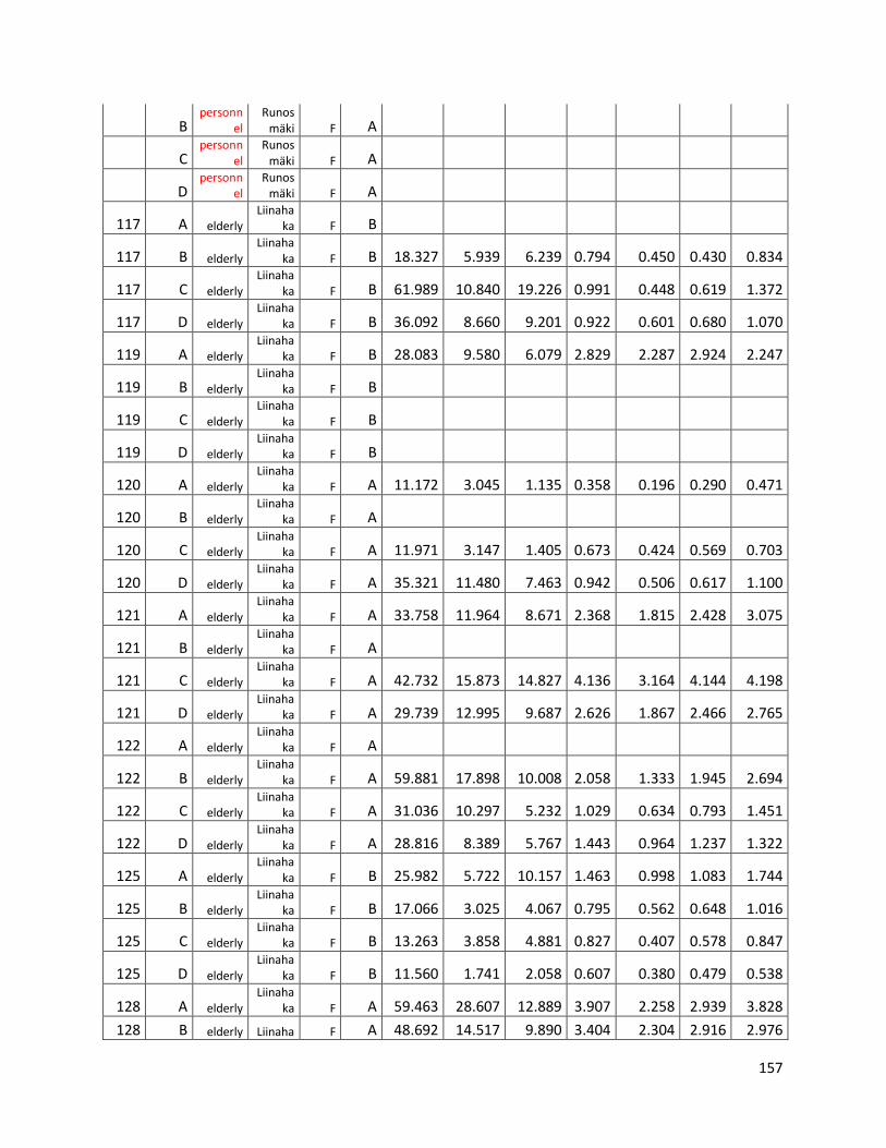
157
B personn
el Runos
mäki F A
C personn
el Runos
mäki F A
D personn
el Runos
mäki F A
117 A elderly Liinaha
ka F B
117 B elderly Liinaha
ka F B 18.327 5.939 6.239 0.794 0.450 0.430 0.834
117 C elderly Liinaha
ka F B 61.989 10.840 19.226 0.991 0.448 0.619 1.372
117 D elderly Liinaha
ka F B 36.092 8.660 9.201 0.922 0.601 0.680 1.070
119 A elderly Liinaha
ka F B 28.083 9.580 6.079 2.829 2.287 2.924 2.247
119 B elderly Liinaha
ka F B
119 C elderly Liinaha
ka F B
119 D elderly Liinaha
ka F B
120 A elderly Liinaha
ka F A 11.172 3.045 1.135 0.358 0.196 0.290 0.471
120 B elderly Liinaha
ka F A
120 C elderly Liinaha
ka F A 11.971 3.147 1.405 0.673 0.424 0.569 0.703
120 D elderly Liinaha
ka F A 35.321 11.480 7.463 0.942 0.506 0.617 1.100
121 A elderly Liinaha
ka F A 33.758 11.964 8.671 2.368 1.815 2.428 3.075
121 B elderly Liinaha
ka F A
121 C elderly Liinaha
ka F A 42.732 15.873 14.827 4.136 3.164 4.144 4.198
121 D elderly Liinaha
ka F A 29.739 12.995 9.687 2.626 1.867 2.466 2.765
122 A elderly Liinaha
ka F A
122 B elderly Liinaha
ka F A 59.881 17.898 10.008 2.058 1.333 1.945 2.694
122 C elderly Liinaha
ka F A 31.036 10.297 5.232 1.029 0.634 0.793 1.451
122 D elderly Liinaha
ka F A 28.816 8.389 5.767 1.443 0.964 1.237 1.322
125 A elderly Liinaha
ka F B 25.982 5.722 10.157 1.463 0.998 1.083 1.744
125 B elderly Liinaha
ka F B 17.066 3.025 4.067 0.795 0.562 0.648 1.016
125 C elderly Liinaha
ka F B 13.263 3.858 4.881 0.827 0.407 0.578 0.847
125 D elderly Liinaha
ka F B 11.560 1.741 2.058 0.607 0.380 0.479 0.538
128 A elderly Liinaha
ka F A 59.463 28.607 12.889 3.907 2.258 2.939 3.828
128 B elderly Liinaha F A 48.692 14.517 9.890 3.404 2.304 2.916 2.976
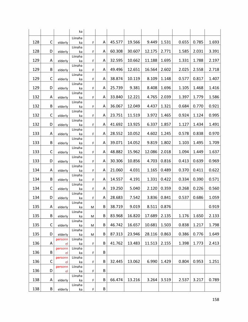
158
ka
128 C elderly Liinaha
ka F A 45.577 19.566 9.449 1.531 0.655 0.785 1.693
128 D elderly Liinaha
ka F A 60.308 30.607 12.175 2.771 1.585 2.031 3.391
129 A elderly Liinaha
ka F A 32.595 10.662 11.188 1.695 1.331 1.788 2.197
129 B elderly Liinaha
ka F A 49.496 12.651 16.564 2.602 2.025 2.558 2.718
129 C elderly Liinaha
ka F A 38.874 10.119 8.109 1.148 0.577 0.817 1.407
129 D elderly Liinaha
ka F A 25.739 9.381 8.408 1.696 1.105 1.468 1.416
132 A elderly Liinaha
ka F A 33.840 12.221 4.765 2.039 1.397 1.779 1.586
132 B elderly Liinaha
ka F A 36.067 12.049 4.437 1.321 0.684 0.770 0.921
132 C elderly Liinaha
ka F A 23.751 11.519 3.972 1.465 0.924 1.124 0.995
132 D elderly Liinaha
ka F A 41.692 13.925 6.337 1.857 1.127 1.434 1.491
133 A elderly Liinaha
ka F A 28.552 10.052 4.602 1.245 0.578 0.838 0.970
133 B elderly Liinaha
ka F A 39.071 14.052 9.819 1.802 1.103 1.495 1.709
133 C elderly Liinaha
ka F A 48.882 15.962 12.086 2.018 1.094 1.449 1.637
133 D elderly Liinaha
ka F A 30.306 10.856 4.703 0.816 0.413 0.639 0.969
134 A elderly Liinaha
ka F A 21.060 4.031 1.165 0.489 0.370 0.411 0.622
134 B elderly Liinaha
ka F A 14.557 4.191 1.331 0.422 0.334 0.390 0.571
134 C elderly Liinaha
ka F A 19.250 5.040 2.120 0.359 0.268 0.226 0.560
134 D elderly Liinaha
ka F A 28.683 7.542 3.836 0.841 0.537 0.686 1.059
135 A elderly Liinaha
ka M B 38.719 9.019 8.511 0.876 0.919
135 B elderly Liinaha
ka M B 83.968 16.820 17.689 2.135 1.176 1.650 2.133
135 C elderly Liinaha
ka M B 46.742 16.657 10.681 1.503 0.838 1.217 1.798
135 D elderly Liinaha
ka M B 87.313 23.946 28.116 0.863 0.386 0.776 1.649
136 A personn
el Liinaha
ka F B 41.762 13.483 11.513 2.155 1.398 1.773 2.413
136 B personn
el Liinaha
ka F B
136 C personn
el Liinaha
ka F B 32.445 13.062 6.990 1.429 0.804 0.953 1.251
136 D personn
el Liinaha
ka F B
138 A elderly Liinaha
ka F B 66.474 13.216 3.264 3.519 2.537 3.217 0.789
138 B elderly Liinaha
ka F B
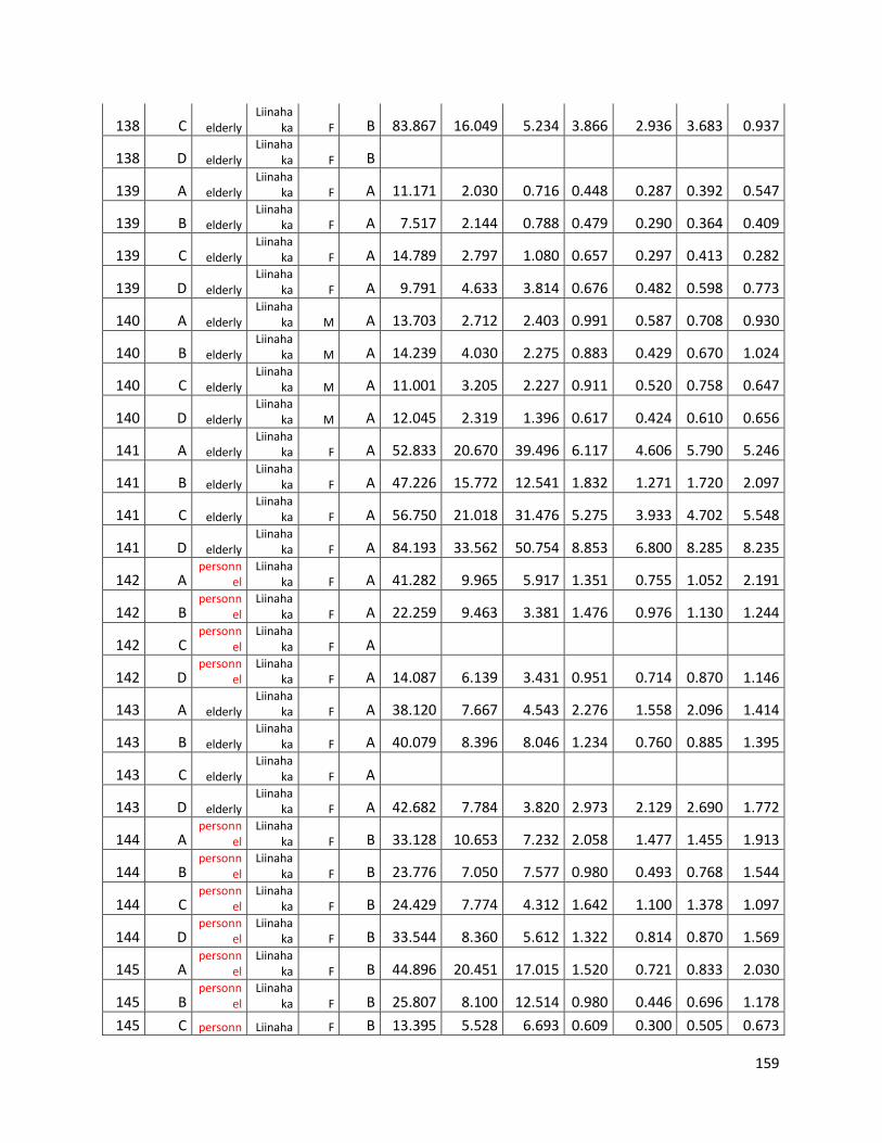
159
138 C elderly Liinaha
ka F B 83.867 16.049 5.234 3.866 2.936 3.683 0.937
138 D elderly Liinaha
ka F B
139 A elderly Liinaha
ka F A 11.171 2.030 0.716 0.448 0.287 0.392 0.547
139 B elderly Liinaha
ka F A 7.517 2.144 0.788 0.479 0.290 0.364 0.409
139 C elderly Liinaha
ka F A 14.789 2.797 1.080 0.657 0.297 0.413 0.282
139 D elderly Liinaha
ka F A 9.791 4.633 3.814 0.676 0.482 0.598 0.773
140 A elderly Liinaha
ka M A 13.703 2.712 2.403 0.991 0.587 0.708 0.930
140 B elderly Liinaha
ka M A 14.239 4.030 2.275 0.883 0.429 0.670 1.024
140 C elderly Liinaha
ka M A 11.001 3.205 2.227 0.911 0.520 0.758 0.647
140 D elderly Liinaha
ka M A 12.045 2.319 1.396 0.617 0.424 0.610 0.656
141 A elderly Liinaha
ka F A 52.833 20.670 39.496 6.117 4.606 5.790 5.246
141 B elderly Liinaha
ka F A 47.226 15.772 12.541 1.832 1.271 1.720 2.097
141 C elderly Liinaha
ka F A 56.750 21.018 31.476 5.275 3.933 4.702 5.548
141 D elderly Liinaha
ka F A 84.193 33.562 50.754 8.853 6.800 8.285 8.235
142 A personn
el Liinaha
ka F A 41.282 9.965 5.917 1.351 0.755 1.052 2.191
142 B personn
el Liinaha
ka F A 22.259 9.463 3.381 1.476 0.976 1.130 1.244
142 C personn
el Liinaha
ka F A
142 D personn
el Liinaha
ka F A 14.087 6.139 3.431 0.951 0.714 0.870 1.146
143 A elderly Liinaha
ka F A 38.120 7.667 4.543 2.276 1.558 2.096 1.414
143 B elderly Liinaha
ka F A 40.079 8.396 8.046 1.234 0.760 0.885 1.395
143 C elderly Liinaha
ka F A
143 D elderly Liinaha
ka F A 42.682 7.784 3.820 2.973 2.129 2.690 1.772
144 A personn
el Liinaha
ka F B 33.128 10.653 7.232 2.058 1.477 1.455 1.913
144 B personn
el Liinaha
ka F B 23.776 7.050 7.577 0.980 0.493 0.768 1.544
144 C personn
el Liinaha
ka F B 24.429 7.774 4.312 1.642 1.100 1.378 1.097
144 D personn
el Liinaha
ka F B 33.544 8.360 5.612 1.322 0.814 0.870 1.569
145 A personn
el Liinaha
ka F B 44.896 20.451 17.015 1.520 0.721 0.833 2.030
145 B personn
el Liinaha
ka F B 25.807 8.100 12.514 0.980 0.446 0.696 1.178
145 C personn Liinaha F B 13.395 5.528 6.693 0.609 0.300 0.505 0.673
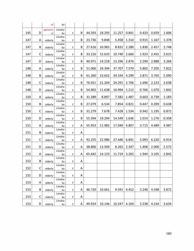
160
el ka
145 D personn
el Liinaha
ka F B 44.593 18.293 11.257 0.841 0.433 0.659 1.606
147 A elderly Liinaha
ka F B 23.736 9.848 5.458 1.310 0.915 1.167 1.378
147 B elderly Liinaha
ka F B 27.616 10.965 8.832 2.280 1.830 2.457 2.748
147 C elderly Liinaha
ka F B 33.216 15.633 10.740 2.660 1.923 2.455 2.615
147 D elderly Liinaha
ka F B 40.971 14.218 13.296 2.876 2.290 2.888 3.268
148 A elderly Liinaha
ka F B 51.060 24.394 37.707 7.579 5.802 7.205 7.822
148 B elderly Liinaha
ka F B 61.260 23.652 34.334 4.299 2.871 3.765 5.090
148 C elderly Liinaha
ka F B 76.921 21.204 34.291 2.706 1.696 2.223 3.638
148 D elderly Liinaha
ka F B 54.902 11.638 16.994 1.212 0.766 1.070 1.842
150 A elderly Liinaha
ka F B 31.289 8.897 7.582 1.487 0.603 0.739 1.183
150 B elderly Liinaha
ka F B 27.079 6.534 7.854 0.821 0.447 0.399 0.638
150 C elderly Liinaha
ka F B 31.279 7.678 7.428 1.534 0.942 1.195 0.872
150 D elderly Liinaha
ka F B 55.394 19.294 14.549 1.636 1.014 1.276 0.358
151 A elderly Liinaha
ka F A 55.953 11.982 17.040 4.807 3.715 4.489 4.987
151 B elderly Liinaha
ka F A
151 C elderly Liinaha
ka F A 92.255 22.986 27.446 6.841 5.093 6.220 6.914
151 D elderly Liinaha
ka F A 38.806 13.509 8.265 2.347 1.408 2.000 2.572
152 A elderly Liinaha
ka F A 65.642 14.123 11.719 3.265 1.944 3.105 2.842
152 B elderly Liinaha
ka F A
152 C elderly Liinaha
ka F A
152 D elderly Liinaha
ka F A
153 A elderly Liinaha
ka F A
153 B elderly Liinaha
ka F A 46.720 10.661 9.591 4.452 3.246 4.598 3.872
153 C elderly Liinaha
ka F A
153 D elderly Liinaha
ka F A 49.924 10.146 10.247 4.169 3.238 4.234 3.634