the effect of financial performance following mergers and ... · pdf filethe effect of...

1

THE EFFECT OF FINANCIAL PERFORMANCE FOLLOWING

MERGERS AND ACQUISITIONS ON FIRM VALUE

Edwin Yonathan, Universitas Indonesia

Ancella A. Hermawan, Universitas Indonesia

2

THE EFFECT OF FINANCIAL PERFORMANCE FOLLOWING

MERGERS AND ACQUISITIONS ON FIRM VALUE

ABSTRACT

The objective of this research is to examine the effect of financial performance following mergers and acquisitions on the firm value. Financial performance is measured from the profitability performance, asset productivity performance, and leverage. Testing hypotheses are conducted using multiple regression models with observations from 120 sample companies listed in Indonesian Stock Exchange that did mergers and acquisitions during the year 2000-2011. The results provide empirical evidence that changes in profitability performance and changes in leverage between the end of fiscal year December 31 closest after and before mergers and acquisitions as well as leverage level and changes in leverage between the end of the book one year after December 31 and before mergers and acquisitions significantly influence the increase of the firm value. Nevertheless, changes of profitability performance, asset productivity performance, leverage level, asset productivity performance between the end of fiscal year December 31 closest after and before mergers and acquisitions and changes of profitability performance, asset productivity performance in profitability performance and changes in asset productivity performance between the end of fiscal year December 31 one year after and before merger and acquisition have no effect on the firm value.

Keywords: mergers and acquisitions, profitability, asset productivity, leverage, firm value.

3

1. INTRODUCTION Growth in gross domestic product (GDP) of Indonesia in 2011 was 6.5% and in 2012 was estimated at 6.1% to 6.5% (Bank Indonesia, 2012), higher than the growth of the world economy. Besides international credit rating agencies, Fitch Ratings and Moody's, respectively at the end of 2011 and beginning of 2012 raised Indonesia's rating after nearly fourteen years since the financial crisis of 1998. Those exposures indicate that the business growth in Indonesia is more quickly and triggers the company to continue to expand its business. However, each company that wants to open or expand its business has limited resources such as competence is not owned, limited access to markets and business scale is not maximized. To overcome these limitations, every company should be able to find and use the right strategies to maintain its survival. One of the recent corporate actions done quite often in order to increase the value of the firm is to do mergers and acquisitions because it can increase the value and efficiency of use of resources so as to be optimal (Weston et al., 2004). Duksaite (2009) said that growth through synergy is a reason / motive of the company's main corporate action to do mergers and acquisitions. Nevertheless in practice, the value creation from synergies that run through merger and acquisition activity is not easy. According to Ficery et al. (2007), some of the factors that led to the synergy were not achieved because the company is too narrow or too broad to define the potential synergies, it missed opportunities synergies that should be obtained, the people have less time to engage in the synergy process, there is mismatch between the system and the culture of the company during the merger and acquisition, and the company uses processes that are less precise in creating synergies. This study will explore how a merger and acquisition affects the financial performance on the firm value. Palepu (2004) said that the first step to analyze the financial performance of the company is to look at the ratio of Return on Equity (ROE). With the du-pont analysis method, ROE is affected by (1) profitability performance, (2) asset productivity performance, and (3) level of leverage. Research conducted by Kumar (2009) in India shows that there is no significant increase before and after a merger in particular in terms of profitability, asset efficiency and solvency. Similar results were also obtained from research conducted by Ooghe et al. (2006) in Belgium. However in Indonesia, Turang (2010) and Initiative (2010) said that there is a significant change in operating income and asset productivity before and after the acquisition. Furthermore, the definition of firm value is the investors’ perception of or expectation from the companies that is often associated with the stock price as the intrinsic value (Price to Book Value (PBV)). The study by Ma et al. (2011) in the United States said that a decline / underperform companies represented value of the ratio of Price to Book (P / BV) between after and before the merger. However Widyaputra (2006) said that there are significant differences in PBV ratios one year after and before the mergers and acquisitions in Indonesia. Thus, this study is aimed to provide empirical evidence about the effect of Indonesia's financial performance after the merger and acquisition on the firm value. 2. LITERATURE REVIEW

4

Recently, merger and acquisition activity is growing. Carbonara and Caiazza (2009) said that since the 1970's era until today, merger and acquisition transactions in the world are growing rapidly not only in the number of transactions but also in scope of companies that undertake mergers and acquisitions between countries (cross-border) and different industries. One contributing factor was an increase in both the world economy, and financial and capital markets in many advanced countries. In Indonesia, the statistical data obtained from Thomson Financial from the Institute of Mergers, Acquisitions and Alliances (2012) showed that there has been an increase in merger and acquisition activity since 1990 with the number of transactions previously under 100 to almost 500 transactions in 2011 and was even reaching over 600 transactions in 2010. This may indicate that merger and acquisition activity is very popular in Indonesia. The reason why companies doing mergers and acquisitions can also be seen from two sides, both the seller and the buyer (Sherman and Hart, 2006). The motivation of why sellers do mergers and acquisitions, among others: the company entered into the business decline, the inability to compete itself, wanted to obtain cost savings through economies of scale and access to resources from the target company. The motivation of why buyers make mergers and acquisitions, among others: increased revenue, cost reduction, vertical and horizontal integration, quality improvement management, growth pressure from investors, increase market share and a desire to diversify their products and services. 2.1. Assessing Financial Performance in Mergers and Acquisitions

The reason why companies are doing mergers and acquisitions as one of the implementation of the corporate strategy is to improve the company’s performance and as an alternative to achieve its business growth. Performance in relation to financial firms both after and before mergers and acquisitions can be viewed by using accounting data and information. Palepu (2004) specifically said the first step to systematically analyze the company’s performance is to use ROE (Return on Equity) as it is a comprehensive indicator. With Du-Pont analysis, ROE can be described as follows:

The figure above showed that the company's financial performance can be seen from three aspects: (1) how companies generate profits from its business activity as measured by NIM (Net Income Margin), (2) how the productivity of the company's assets generate sales levels, measured from TATO (Total Asset Turnover), and (3) how the company fund their assets, measured by DER (Debt to Equity ratio). The pattern that performs financial measurement is

5

similar to that of research conducted by Feroz (2005), using a model of DEA (Data Envelopment Analysis). DEA evaluates the company by looking at the input and output through ratio analysis. The company is said to be effective if the management is able to manage the business to generate maximum output with minimum input. By taking the example of the same ratio, ROE, the company is said to be effective if the minimum sales, total assets and equity are able to produce maximum returns (net income). Profitability is an important measurement in assessing the company’s performance. This was confirmed by Singh and Mogla (2010) who said that basically mergers and acquisitions occur because of a desire to maximize profits / profitability and growth. Previous researches have linked profitability performance with merger and acquisition activity. Ooghe et al. (2006) in Belgium said that the profitability level of the acquirer is not in line with the acquisition objectives. Similar results were also presented by Kumar (2009) for his research on companies in India within a period of three years before and after mergers and acquisitions. However, Turang (2010) said that there is a significant change to the operating profit for companies in Indonesia doing mergers and acquisitions over the past five years. Every company requires assets to support their business activities. Managing resources of company’s assets and using them for business operations are factors affecting the financial performance. Ross (2010) said that the company needs to look at how effective and efficient the asset management is by using the asset management. Previous researches have linked asset productivity performance with merger and acquisition activity. Prakarsa (2009) in Indonesia said that there is a significant change from the asset management represented by TATO in the two years before and after mergers and acquisitions. However, Singh and Mogla (2010) and Kumar (2009) said that there is a decline in asset utilization after a merger and acquisition firms in India. Assets required supporting the business activities need to be funded. Leverage could come from shareholders or debt where the same purpose remains, to increase the company value. If the company uses debt to finance the company, it means the firm uses leverage. Modligani and Miller (1963) said that companies using debt in their capital structure will benefit due to the tax shield which can then increase the company value. Previous studies have linked the level of leverage (leverage) with merger and acquisition activity. Ghosh and Jain (2000) said that there is a significant increase in the financial leverage of the companies that merged in the United States. It is also said by Huang (2010) in China that there is a significant increase in financial leverage following the acquisition. However, it is not the case in India (Kumar, 2009) and in Indonesia (Initiative, 2010 and Turang, 2010). 2.2. Assessing Firm Value in Mergers and Acquisitions Firm value is the investor's perception of the company that is often associated with stock prices (Fama, 1978). High stock price makes the company value also high. Stock market price is formed between buyers and sellers (demand and supply) at the transaction called market value. In connection with mergers and acquisitions, Mogla and Singh (2010) said that assessing the performance of mergers and acquisitions can be seen from accounting data and market data. However, market data especially the stock price is believed to be more reliable because it is in line with the theory and concept of efficient capital markets. Damodaran (2002) said that the use

6

Div1 r - g

BV0 X ROE X Payout Ratio X (1 + g) r - g

Div1 r - g

ROE X Payout Ratio X (1 + g) r - g

P0 BV0

of PBV (Price to Book Value) as one of the financial ratios is sufficiently representative to see the performance in terms of creation of value for the company. It is also said by Block (1995) that the PBV ratio is very important because it describes the external and internal factors of the share price, which reflects the market cycle and firm. Research conducted by Kruse et al. (2007) said that the long-term performance of the company improved significantly after the merger and acquisition by seeing an increase in the rate of return of the stock price changes in Japan. In particular, this is due to many Japanese companies are diversified. Similar results were also expressed by Soongswang (2010) in Thailand who said that mergers and acquisitions affect the creation of shareholder wealth. On the contrary, DeLong (2003) said that there is no significant increase in regards of the stock market reaction to merger and acquisition transactions. This is because the market is very difficult to make projections of a success of mergers and acquisitions made in the United States. 2.3. The Effect of Financial Performance on Firm Value Damodaran (2002) tried to relate ROE with PBV. If the company is assumed to have a constant growth rate, the intrinsic value of shares can be expressed by the following equation: P0 = Where : P0 = value of equity per share today Div1 = expected dividends per share next year r = discount rate (cost of equity) g = growth rate constant Because dividends can be expressed as the company's book value (BV) multiply by ROE and dividend payout ratio, the equation above can be written as follows: P0 = = If both sides of the equation are divided by BV0 and assuming that the intrinsic value is equal to the stock price, then the above equation can be expressed as follows:

PBV = = The equation above shows that ROE affects PBV. In accordance with the du-pont in the ROE, it can be said that the profitability performance, asset productivity performance and level of leverage affect the expectations of the market as represented by PBV. 3. HYPOTHESIS DEVELOPMENT In general, the hypothesis of this study is to prove whether the financial performance has positive effect on the firm value represented by the ratio of Price to Book Value (PBV). Damodaran (2002) relates ROE and PBV, stating that the higher the ROE, the higher the PBV. While ROE is influenced by the profitability performance as represented by Net Income Margin (NIM), asset

7

productivity performance is represented by the Total Asset Turnover (TATO) and level of leverage is represented by the Debt to Equity Ratio (DER). 3.1. Profitability Performance In connection with mergers and acquisitions, Mogla Singh (2010) said that basically mergers and acquisitions are done due to the desire to maximize profit / profitability and growth. The advantages achieved by the company ultimately increase shareholder wealth by the distribution of dividends. Bodie et al. (2011) said that the intrinsic value of stock is the sum of the present value of expected cash flows received by the shareholders in the future in the form of dividends. Value of the shares which is the concept of intrinsic value represents the company value. Thus, the higher the profitability performance is, the higher the firm value will be. Therefore, the first hypotheses of this research are: H1a.1: Profitability performance after mergers and acquisitions has a positive effect on its PBV

ratio. H1a.2: Changes in profitability performance after and before mergers and acquisitions have a

positive effect on its PBV ratio. 3.2. Asset Productivity Performance In connection with mergers and acquisitions, Mogla Singh (2010) also said that mergers and acquisitions will certainly increase the company size. This means that management must be careful in managing their assets more effectively and efficiently in order to generate increased sales, while increased assets also lead to increased costs in terms of maintenance and depreciation expense. Brush et al. (2000) said that the higher the sales growth of the company is, the greater the increase in the company's performance will be. Thus, the higher asset productivity performance is, the higher the firm value will be. Therefore, the second hypotheses of this research are: H2a.1: Asset productivity performance after mergers and acquisitions has a positive effect on its

PBV ratio. H2a.2: Change in asset productivity performance after and before mergers and acquisitions have

positive effect on its PBV ratio. 3.3. Leverage Modligani and Miller (1963) said that companies using debt in their capital structure will benefit due to the tax shield which can increase the company value. However, there is no specific target in regards of how much influence of DER ratio to increase the corporate value. In connection with mergers and acquisitions, Ghosh and Jain (2000) said that empirically, firms increase their financial leverage through merger activity by increasing debt capacity in order to increase shareholder wealth by exploiting tax shield. Therefore, the third hypotheses of this research are: H3a.1: Leverage level after mergers and acquisitions has a positif effect on its PBV ratio.

8

H3a.2: Changes in leverage level after and before mergers and acquisitions have a positive effect on its PBV ratio.

4. RESEARCH MODEL The model used in this research is the development of the model of Kumar (2009) and Huang (2010). This research is to examine the effect of financial performance following mergers and acquisitions on the firm value. In addition, several control variables that have been shown to affect the firm value, the company's risk and the sales growth rate, are included in this research model. � Model A: profitability performance tested separately

PBVi = β0 + β1 NIM i + β2 Diff_NIM i + β3 RISK i + β4 Diff_RISK i + β5 GROWTH i + β6 Diff_GROWTH i + β7 IND_KONSUMSI i + β8 IND_DASARi + β9 IND_INFRA i + β10 IND_DAGANG i + β11 IND_TANI i + β12 IND_PROPERTI i + β13 IND_ANEKA i + ei

� Model B: asset productivity performance tested separately

PBVi = β0 + β1 TATO i + β2 Diff_TATO i + β3 RISK i + β4 Diff_RISK i + β5 GROWTH i + β6 Diff_GROWTH i + β7 IND_KONSUMSI i + β8 IND_DASARi

+ β9 IND_INFRA i + β10 IND_DAGANG i + β11 IND_TANI i + β12 IND_PROPERTI i + β13 IND_ANEKA i + ei

� Model C: leverage level tested separately

PBVi = β0 + β1 DERi + β2 Diff_DER i + β3 RISK i + β4 Diff_RISK i + β5 GROWTH i + β6 Diff_GROWTH i + β7 IND_KONSUMSI i + β8 IND_DASARi + β9 IND_INFRA i + β10 IND_DAGANG i + β11 IND_TANI i + β12 IND_PROPERTI i + β13 IND_ANEKA i + ei

� Model D: all financial performance variables tested together

PBVi = β0 + β1 NIM i + β2 Diff_NIM i + β3 TATO i + β4 Diff_TATO i + β5 DERi + β6 Diff_DER i + β7 RISK i + β8 Diff_RISK i + β9 GROWTH i + β10 Diff_GROWTH i + β11 IND_KONSUMSI i + β12 IND_DASARi + β13 IND_INFRA i + β14 IND_DAGANG i + β15 IND_TANI i + β16 IND_PROPERTI i + β17 IND_ANEKA i + ei

Where: PBVi : Price to Book Value (PBV) ratio of firm i at the end of the period after

the mergers and acquisitions. NIM i : Net Income Margin (NIM) ratio of firm i at the end of the period after

the mergers and acquisitions. Diff_NIM i : Changes between NIM ratios of firm i at the end of the period after the

mergers and acquisitions and average three years before mergers and

9

acquisitions. TATOi : Total Asset Turnover (TATO) ratio of firm i at the end of the period

after the mergers and acquisitions. Diff_TATO i : Changes between TATO ratios of firm i at the end of the period after the

mergers and acquisitions and average three years before mergers and acquisitions.

DERi : Debt to Equity (DER) ratio of firm i at the end of the period after the mergers and acquisitions.

Diff_DERi : Changes between DER ratios of firm i at the end of the period after the


RISKi : Firm risk measured by the beta of firm i at the end of the period after the

mergers and acquisitions Diff_RISKi : Changes between the betas of firm i at the end of the period after the


GROWTHi : Sales growth rate of firm i at the end of the period after the mergers and

acquisitions. Diff_GROWTHi : Changes between sales growth rates of firm i at the end of the period

after the mergers and acquisitions and average three years before mergers and acquisitions.

IND_KONSUMSIi : Type of industry is measured using dummy variable (1,0) with value of 1

if firm 1 is classified as consumer goods industry. IND_DASARi : Type of industry is measured using dummy variable (1,0) with value of 1

if firm 1 is classified as basic industry and chemicals. IND_INFRAi : Type of industry is measured using dummy variable (1,0) with value of 1

if firm 1 is classified as infrastructure, utility and transportation industry. IND_DAGANGi : Type of industry is measured using dummy variable (1,0) with value of 1

if firm 1 is classified as trade, services & investment industry. IND_TANI i : Type of industry is measured using dummy variable (1,0) with value of 1

if firm 1 is classified as agriculture industry. IND_PROPERTIi : Type of industry is measured using dummy variable (1,0) with value of 1

10

if firm 1 is classified as property and real estate industry. IND_ANEKA i : Type of industry is measured using dummy variable (1,0) with value of 1

if firm 1 is classified as miscellaneous industry. In this model, the end of the period after the mergers and acquisitions means the end of fiscal year on December 31, closest after the mergers and acquisitions which is denoted as year t (model 1) and the end of fiscal year on December 31, one year after the mergers and acquisitions which is denoted as year t +1 (model 2). 5. POPULATION AND SAMPLE The population of this study consists of all companies listed in the Indonesia Stock Exchange (IDX) that had mergers and acquisitions activity during 2000 to 2011. Using a purposive sampling method, there are 120 firms that meet all the criteria in this study. Table 1 shows the sample determination in this study and Table 2 shows the sample profile based on industry.

Table 1. Determination of Sample Step Sample Criteria Number of

Companies 1 Companies that had mergers and acquisitions,

excluding financial industry, listed in the Indonesian Stock Exchange (IDX) during 2000-2009

155

2 Companies that have negative equity (10) 3 Companies that have incomplete data (25) Total samples used 120

Of the 120 sample firms, approximately 108 companies or as much as 90% of the samples were acquired and 12 companies or 10% were merged. Thus, the analysis of this study reflects the result of the acquisition transaction only.

Table 2. Sample Profile Based on Industry No. Industries Number of

Companies Percentage

1. Consumer goods 11 9.17% 2. Basic industry and chemicals 16 13.33% 3. Infrastructure, utility and transportation 12 10.00% 4. Trade, services & investment 29 24.16% 5. Mining 17 14.17% 6. Agriculture 9 7.50% 7. Property and Real Estate 17 14.17% 8. Miscelaneous 9 7.50% Total 120 100.00%

11

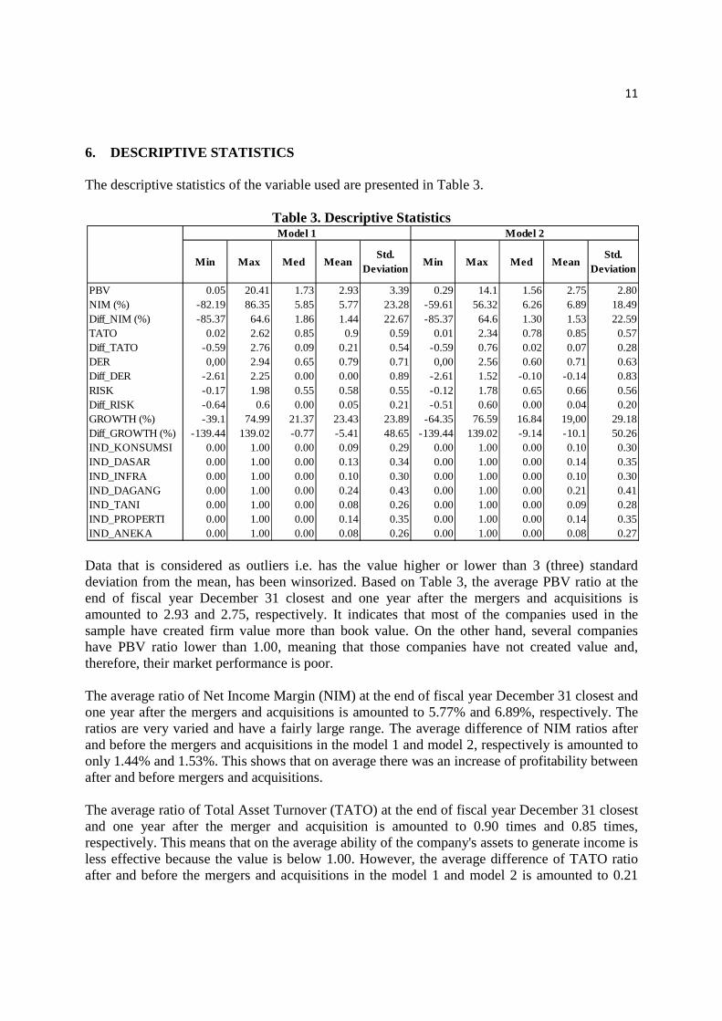
6. DESCRIPTIVE STATISTICS The descriptive statistics of the variable used are presented in Table 3.

Table 3. Descriptive Statistics

Data that is considered as outliers i.e. has the value higher or lower than 3 (three) standard deviation from the mean, has been winsorized. Based on Table 3, the average PBV ratio at the end of fiscal year December 31 closest and one year after the mergers and acquisitions is amounted to 2.93 and 2.75, respectively. It indicates that most of the companies used in the sample have created firm value more than book value. On the other hand, several companies have PBV ratio lower than 1.00, meaning that those companies have not created value and, therefore, their market performance is poor. The average ratio of Net Income Margin (NIM) at the end of fiscal year December 31 closest and one year after the mergers and acquisitions is amounted to 5.77% and 6.89%, respectively. The ratios are very varied and have a fairly large range. The average difference of NIM ratios after and before the mergers and acquisitions in the model 1 and model 2, respectively is amounted to only 1.44% and 1.53%. This shows that on average there was an increase of profitability between after and before mergers and acquisitions. The average ratio of Total Asset Turnover (TATO) at the end of fiscal year December 31 closest and one year after the merger and acquisition is amounted to 0.90 times and 0.85 times, respectively. This means that on the average ability of the company's assets to generate income is less effective because the value is below 1.00. However, the average difference of TATO ratio after and before the mergers and acquisitions in the model 1 and model 2 is amounted to 0.21

Min Max Med MeanStd.

DeviationMin Max Med Mean

Std. Deviation

PBV 0.05 20.41 1.73 2.93 3.39 0.29 14.1 1.56 2.75 2.80NIM (%) -82.19 86.35 5.85 5.77 23.28 -59.61 56.32 6.26 6.89 18.49Diff_NIM (%) -85.37 64.6 1.86 1.44 22.67 -85.37 64.6 1.30 1.53 22.59TATO 0.02 2.62 0.85 0.9 0.59 0.01 2.34 0.78 0.85 0.57Diff_TATO -0.59 2.76 0.09 0.21 0.54 -0.59 0.76 0.02 0.07 0.28DER 0,00 2.94 0.65 0.79 0.71 0,00 2.56 0.60 0.71 0.63Diff_DER -2.61 2.25 0.00 0.00 0.89 -2.61 1.52 -0.10 -0.14 0.83RISK -0.17 1.98 0.55 0.58 0.55 -0.12 1.78 0.65 0.66 0.56Diff_RISK -0.64 0.6 0.00 0.05 0.21 -0.51 0.60 0.00 0.04 0.20GROWTH (%) -39.1 74.99 21.37 23.43 23.89 -64.35 76.59 16.8419,00 29.18Diff_GROWTH (%) -139.44 139.02 -0.77 -5.41 48.65 -139.44 139.02 -9.14 -10.1 50.26IND_KONSUMSI 0.00 1.00 0.00 0.09 0.29 0.00 1.00 0.00 0.10 0.30IND_DASAR 0.00 1.00 0.00 0.13 0.34 0.00 1.00 0.00 0.14 0.35IND_INFRA 0.00 1.00 0.00 0.10 0.30 0.00 1.00 0.00 0.10 0.30IND_DAGANG 0.00 1.00 0.00 0.24 0.43 0.00 1.00 0.00 0.21 0.41IND_TANI 0.00 1.00 0.00 0.08 0.26 0.00 1.00 0.00 0.09 0.28IND_PROPERTI 0.00 1.00 0.00 0.14 0.35 0.00 1.00 0.00 0.14 0.35IND_ANEKA 0.00 1.00 0.00 0.08 0.26 0.00 1.00 0.00 0.08 0.27

Model 1 Model 2

12

times and 0.07 times, respectively. This shows that on average there was an increase in asset productivity between before and after mergers and acquisitions. The average of Debt to Equity Ratio (DER) at the end of fiscal year December 31 closest and one year after the mergers and acquisitions is amounted to 0.79 times and 0.71 times, respectively. This means that on average companies prefer to use equity rather than debt to fund their assets. In addition, there was no difference in the average DER ratio after and before mergers and acquisitions in models 1 and even become -0.14 times in model 2 which shows that the portion of debt to equity tends to decrease after the mergers and acquisitions. The difference in the average ratio of DER does not have a large range on this sample. The average value of beta at the end of fiscal year December 31 closest and one year after the mergers and acquisitions is amounted to 0.58 and 0.66, respectively, which means that on average, the samples observed have a lower risk than the market risk because the value is below 1.00 even though it is unidirectional to market risks. The average value of a lower beta can be caused by the presence of several stocks of companies that are not actively traded in the stock exchange during the research period. The difference in the average beta values after and before mergers and acquisitions is very small, amounted to 0.05 and 0.04, respectively in model 1 and model 2 and has a very small range on this sample. The average growth rate of sales in the fiscal year December 31 closest and one year after the mergers and acquisitions is amounted to 23.43% and 19.00%. The ratio has a fairly large range. However, the difference in the average rate of growth in sales after and before mergers and acquisitions in the model 1 and model 2 is amounted to -5.41% and -10.10%, respectively. This shows that on average there was a decline in sales growth between after and before mergers and acquisitions. 7. CORRELATION ANALYSIS The correlation analysis results for model 1 and model 2 are presented in Table 4.1 and Table 4.2, respectively. The value of the dependent variable in the correlation analysis is the result of transformation (LogPBV) in order to meet the normality assumption of regression models. From the six main variables in model 1, only Diff_NIM was correlated positively and significantly with LogPBV. This means that the higher the ratio of the average difference between the end of fiscal year NIM December 31 closest after the mergers and acquisitions and an average three years of NIM before mergers and acquisitions, the greater the PBV ratio. While in model 2, the overall main variable has no significant LogPBV. Of the four control variables, only variables and Diff_GROWTH Diff_RISK have positive and significant correlation LogPBV in both model 1 and model 2. This means that the higher the difference in the average value of beta and the difference in the average rate of sales growth between the end of fiscal year December 31 closest and one year after the mergers and acquisitions, and an average over the three years before to mergers and acquisitions, the greater the PBV ratio value. While in regards of the entire industry dummy variables, none of the significant industries has correlation LogPBV both in the model 1 and model 2. Correlation

13

coefficients between all independent variables are relatively small i.e. below 0.80. This indicates the small possibility of multicollinearity in the regression results in this research model.

17

Table 4.1. Pearson Correlation Analysis (Model 1)

Model 1 LogPBV NIMDiff_NIM

TATODiff_ATO

DERDiff_DER

RISKDiff_RISK

GROWTHDiff_

GROWTHIND_KONSUMSI

IND_DASAR

IND_INFRA

IND_DAGANG

IND_TANI

IND_PROPERTI

IND_ANEKA

1,000

0,108 1,000

(0,241)0,230* 0,098 1,000

(0,011) (0,285)0,089 0,112 0,003 1,000

(0,331) (0,222) (0,973)0,042 0,069 0,063 0,429** 1,000

(0,646) (0,452) (0,493) (0,000)0,107 -0,255** -0,093 -0,010 -0,021 1,000

(0,243) (0,005) (0,313) (0,916) (0,819)-0,069 0,053 -0,227* 0,099 0,297** 0,122 1,000

(0,456) (0,566) (0,013) (0,284) (0,001) (0,183)0,055 0,233* -0,058 0,125 -0,166 -0,184* -0,164 1,000

(0,547) (0,010) (0,530) (0,172) (0,070) (0,044) (0,073)0,191* 0,076 -0,040 0,099 0,107 0,021 0,124 0,227* 1,000

(0,037) (0,407) (0,666) (0,282) (0,245) (0,822) (0,178) (0,013)0,083 0,341** 0,043 0,124 0,165 0,028 0,152 0,067 0,187* 1,000

(0,370) (0,000) (0,638) (0,177) (0,071) (0,760) (0,096) (0,466) (0,041)0,311** -0,077 0,087 0,169 0,266** 0,141 0,222* -0,188* -0,018 -0,088 1,000

(0,001) (0,404) (0,343) (0,065) (0,003) (0,123) (0,015) (0,040) (0,841) (0,338)0,027 -0,077 0,000 0,042 -0,127 0,089 -0,073 0,087 -0,058 -0,060 0,136 1,000

(0,772) (0,404) (0,997) (0,649) (0,166) (0,335) (0,425) (0,343) (0,526) (0,513) (0,137)0,000 -0,018 0,112 0,184* 0,104 0,069 -0,125 0,077 -0,084 -0,066 0,051 -0,125 1,000

(0,999) (0,843) (0,224) (0,044) (0,258) (0,451) (0,175) (0,406) (0,360) (0,475) (0,577) (0,175)0,100 0,028 -0,028 -0,177 -0,027 0,097 0,157 -0,230* -0,062 0,067 0,029 -0,106 -0,131 1,000

(0,277) (0,760) (0,761) (0,053) (0,768) (0,292) (0,086) (0,011) (0,498) (0,468) (0,753) (0,250) (0,155)-0,125 0,011 -0,080 0,146 0,155 -0,036 0,138 -0,165 0,158 0,062 0,051 -0,179 -0,221* -0,188* 1,000

(0,175) (0,905) (0,382) (0,112) (0,090) (0,695) (0,133) (0,071) (0,086) (0,503) (0,582) (0,050) (0,015) (0,040)-0,112 0,124 -0,068 -0,076 -0,064 -0,060 -0,097 0,118 0,064 0,113 -0,095 -0,090 -0,112 -0,095 -0,161 1,000(0,223) (0,175) (0,458) (0,406) (0,484) (0,515) (0,291) (0,201) (0,489) (0,217) (0,302) (0,326) (0,225) (0,302) (0,079)-0,125 -0,018 0,102 -0,346** -0,096 -0,228* -0,082 0,045 -0,179 -0,021 -0,231* -0,129 -0,159 -0,135 -0,229* -0,116 1,000(0,174) (0,843) (0,266) (0,000) (0,299) (0,012) (0,372) (0,628) (0,051) (0,821) (0,011) (0,160) (0,082) (0,140) (0,012) (0,208)-0,098 0,024 0,025 0,234* 0,045 -0,133 0,031 0,024 -0,056 -0,011 0,048 -0,090 -0,112 -0,095 -0,161 -0,081 -0,116 1,000(0,286) (0,798) (0,790) (0,010) (0,628) (0,146) (0,735) (0,797) (0,546) (0,907) (0,602) (0,326) (0,225) (0,302) (0,079) (0,379) (0,208)

GROWTH

LogPBV

NIM

Diff_NIM

TATO

Diff_TATO

DER

Diff_DER

RISK

Diff_RISK

Diff_GROWTH

IND_ANEKA

IND_KONSUMSI

IND_DASAR

IND_INFRA

IND_DAGANG

IND_TANI

IND_PROPERTI

* Signnificant at the level α = 5% (2-tailed) ** Significant at the level α = 1% (2-tailed) Amount in the bracket is the p-value

18

Table 4.2. Pearson Correlation Analysis (Model 2)

Model 2 LogPBV NIMDiff_NIM

TATODiff_ATO

DERDiff_DER

RISKDiff_RISK

GROWTHDiff_

GROWTHIND_KONSUMSI

IND_DASAR

IND_INFRA

IND_DAGANG

IND_TANI

IND_PROPERTI

IND_ANEKA

1

0,042 1,000

(0,672)0,068 0,565** 1,000

(0,495) (0,000)0,023 0,002 -0,018 1,000

(0,818) (0,986) (0,855)-0,089 0,008 0,084 0,409** 1,000

(0,369) (0,935) (0,394) (0,000)0,174 -0,198* 0,114 -0,054 0,113 1,000

(0,077) (0,044) (0,251) (0,584) (0,253)-0,141 -0,334** -0,204* 0,143 0,235* 0,272** 1,000

(0,154) (0,001) (0,038) (0,149) (0,016) (0,005)0,072 0,249* -0,001 0,173 0,010 -0,180 -0,104 1,000

(0,466) (0,011) (0,992) (0,080) (0,916) (0,067) (0,296)0,193* 0,010 0,032 0,080 0,042 -0,004 0,051 0,273** 1,000(0,049) (0,922) (0,750) (0,422) (0,673) (0,971) (0,606) (0,005)

0,157 0,105 0,005 0,109 0,210* -0,056 -0,024 -0,019 -0,019 1,000

(0,112) (0,291) (0,958) (0,269) (0,033) (0,574) (0,810) (0,851) (0,851)0,306** 0,043 0,109 0,335** 0,288** 0,161 0,145 -0,147 -0,073 0,288** 1,000

(0,002) (0,662) (0,271) (0,001) (0,003) (0,102) (0,143) (0,137) (0,464) (0,003)0,138 -0,101 -0,012 0,099 -0,134 -0,041 -0,096 0,063 -0,093 0,045 0,167 1,000

(0,163) (0,306) (0,904) (0,318) (0,175) (0,682) (0,333) (0,527) (0,348) (0,647) (0,090)-0,053 0,036 0,123 0,227* 0,262** 0,053 -0,092 0,089 -0,067 0,035 0,086 -0,134 1,000

(0,595) (0,718) (0,215) (0,021) (0,007) (0,596) (0,352) (0,369) (0,501) (0,721) (0,388) (0,175)0,010 -0,212* -0,072 -0,166 0,040 0,098 0,219* -0,238* -0,041 -0,154 0,004 -0,106 -0,134 1,000

(0,919) (0,031) (0,469) (0,093) (0,683) (0,320) (0,026) (0,015) (0,679) (0,118) (0,970) (0,282) (0,175)-0,164 -0,051 -0,037 0,097 -0,019 0,046 0,109 -0,188 0,120 -0,120 0,020 -0,169 -0,213* -0,169 1,000

(0,095) (0,605) (0,712) (0,325) (0,850) (0,641) (0,269) (0,056) (0,225) (0,225) (0,843) (0,086) (0,030) (0,086)0,031 -0,050 -0,075 -0,016 0,025 0,046 -0,062 0,134 0,114 0,011 -0,071 -0,100 -0,126 -0,100 -0,159 1,000

(0,758) (0,611) (0,446) (0,868) (0,799) (0,643) (0,534) (0,174) (0,247) (0,913) (0,476) (0,311) (0,201) (0,311) (0,106)-0,186 0,291** 0,109 -0,382** -0,108 -0,135 -0,141 0,066 -0,177 0,135 -0,266** -0,134 -0,169 -0,134 -0,213* -0,126 1,000(0,059) (0,003) (0,272) (0,000) (0,277) (0,171) (0,153) (0,507) (0,072) (0,172) (0,006) (0,175) (0,087) (0,175) (0,030) (0,201)-0,130 0,018 0,013 0,275** 0,111 -0,072 0,058 -0,047 -0,148 0,007 0,059 -0,094 -0,119 -0,094 -0,150 -0,089 -0,119 1,000(0,190) (0,858) (0,897) (0,005) (0,263) (0,465) (0,556) (0,637) (0,135) (0,947) (0,552) (0,342) (0,231) (0,342) (0,130) (0,370) (0,231)

IND_DAGANG

IND_TANI

IND_PROPERTI

IND_ANEKA

GROWTH

Diff_GROWTH

IND_KONSUMSI

IND_DASAR

IND_INFRA

Diff_TATO

DER

Diff_DER

RISK

Diff_RISK

LogPBV

NIM

Diff_NIM

TATO

* Signnificant at the level α = 5% (2-tailed) ** Significant at the level α = 1% (2-tailed) Amount in the bracket is the p-value

19

8. HYPOTHESIS TESTING ANALYSIS 8.1. The Effect of Profitability Performance on The Firm Value Based on the regression results in Table 5.1 and Table 5.2, NIM does not have any significant effect on the PBV ratio in both models 1A and 2A. This is similar when testing all of the main variables together (with asset productivity performance and level of leverage) in both models 1D and 2D. The results showed that increased ratio of NIM at the end of fiscal year December 31 closest or one year after the merger and acquisitions was not significant on the firm value. This result is also a representation of the acquisition transaction because based on the regression results in Table 5.2 and Table 5.4, the results are similar. Thus, these results do not support hypothesis 1a.1, and therefore, the hypothesis is rejected in both models 1 and 2. These results are consistent with the finding of Ooghe et al. (2006) in Belgium which stated that the level of profitability of the acquirer is not in line with the objectives of the acquisition. Furthermore, based on the regression results in Table 5, Diff_NIM has significant effect on the PBV ratio in model 1A. This is similar when testing all of the main variables together (with asset productivity performance and level of leverage) in model 1D. The results showed that differences in NIM ratio at the end of fiscal year on December 31 after the merger and acquisition closest and the average NIM ratios for three years before the mergers and acquisitions have significant effect on the firm value. This result is also a representation of the acquisition transaction because based on the regression results in Table 5.2, the results are similar. Thus, model 1 results support hypothesis 1a.2, and therefore, the hypothesis cannot be rejected. These results are similar to that of research conducted by Turang (2010) which said that there is a significant change to the operational profit for companies in Indonesia that did mergers and acquisitions.

20

Table 5.1. Regression Output (Model 1 – Mergers and Acquisitions)

Unstandardized

Coefficientst-Statistic

Unstandardized


Unstandardized


Unstandardized

Coefficients

B B B B(Constant) 0,564 7,748 0,000 0,523 6,349 0,000 0,554 6,397 0,000 0,517 5,581 0,000

NIM + 0,001 0,975 0,165 - - - - - - 0,001 1,139 0,129Diff_NIM + 0,002 2,597 0,005* - - - - - - 0,002 2,049 0,022**

TATO + - - - 0,049 0,928 0,178 - - - 0,047 0,921 0,180Diff_TATO + - - - -0,045 -0,827 0,205 - - - -0,029 -0,542 0,294DER + - - - - - - 0,003 0,072 0,471 0,015 0,390 0,349Diff_DER + - - - - - - 0,068 2,340 0,011** 0,053 1,718 0,044**

RISK - 0,034 0,703 0,241 0,024 0,477 0,317 0,026 0,521 0,302 0,015 0,295 0,384Diff_RISK - 0,193 1,597 0,056** 0,204 1,623 0,054* 0,224 1,822 0,036** 0,227 1,857 0,033**

GROWTH + 0,001 0,776 0,219 0,001 1,275 0,103 0,002 1,662 0,050 ** 0,001 0,907 0,183Diff_GROWTH + 0,001 3,583 0,002*** 0,002 3,726 0,000*** 0,002 4,227 0,000*** 0,002 3,833 0,000***

IND_KONSUMSI + 0,228 2,273 0,012** 0,237 2,268 0,013** 0,242 2,376 0,010*** 0,245 2,422 0,009***

IND_DASAR + 0,247 2,721 0,003*** 0,224 2,368 0,010*** 0,238 2,590 0,005*** 0,261 2,823 0,003***

IND_INFRA + 0,127 1,264 0,104 0,113 1,079 0,142 0,102 0,995 0,161 0,098 0,963 0,169IND_DAGANG + 0,299 3,755 0,001*** 0,302 3,647 0,000*** 0,293 3,551 0,000*** 0,293 3,580 0,000***

IND_TANI + 0,333 3,113 0,001*** 0,324 2,930 0,002*** 0,352 3,213 0,001*** 0,338 3,102 0,001***

IND_PROPERTI + 0,263 2,867 0,002*** 0,212 2,166 0,016** 0,239 2,484 0,007*** 0,228 2,313 0,011**

IND_ANEKA + 0,343 3,221 0,001*** 0,345 3,061 0,001*** 0,323 2,917 0,002*** 0,347 3,107 0,001***

R-squared 0,328 0,282 0,311 0,355Adjusted R-squared 0,246 0,194 0,226 0,247F-statistic 3,980 3,202 3,673 3,302Prob (F-statistic) 0.000 0.000 0.000 0.000

t-StatisticVariabel

Expected Sign

Model 1DModel 1B Model 1CModel 1A

Sig.Sig. Sig. Sig.

* Significant at the level α = 10% (1-tailed) ** Significant at the level α = 5% (1-tailed) *** Significant at the level α = 1% (1-tailed)

21

Table 5.2. Regression Output (Model 1 – Acquisitions)

Unstandardized


Unstandardized


Unstandardized


Unstandardized

CoefficientsB B B B

(Constant) 0,499 6,426 0,000 0,473 5,497 0,000 0,492 5,520 0,000 0,487 5,119 0,000NIM + 0,001 0,970 0,167 - - - - - - 0,001 1,112 0,134Diff_NIM + 0,003 2,398 0,009*** - - - - - - 0,002 1,662 0,050**

TATO + - - - 0,020 0,353 0,362 - - - 0,012 0,231 0,409Diff_TATO + - - - -0,032 -0,582 0,281 - - - -0,012 -0,219 0,414DER + - - - - - - 0,018 -0,466 0,321 0,001 0,023 0,491Diff_DER + - - - - - - 0,085 -2,805 0,003*** 0,071 2,206 0,015**

RISK - 0,058 1,077 0,142 0,051 0,918 0,181 0,047 0,880 0,190 0,043 0,773 0,221Diff_RISK - 0,212 1,732 0,043** 0,220 1,721 0,044** 0,245 2,001 0,024** 0,247 2,004 0,024**

GROWTH + 0,000 0,307 0,380 0,001 0,777 0,219 0,001 1,292 0,110 0,001 0,701 0,243Diff_GROWTH + 0,002 3,745 0,000*** 0,002 3,860 0,000*** 0,002 4,562 0,000*** 0,002 4,151 0,000***

IND_KONSUMSI + 0,190 1,765 0,040** 0,189 1,679 0,048** 0,191 1,789 0,038** 0,199 1,843 0,034**

IND_DASAR + 0,172 1,762 0,041** 0,140 1,372 0,087* 0,149 1,545 0,063* 0,174 1,757 0,041**

IND_INFRA + 0,053 0,507 0,307 0,040 0,370 0,356 0,014 0,137 0,446 0,028 0,267 0,395IND_DAGANG + 0,222 2,542 0,006*** 0,217 2,360 0,010*** 0,204 2,302 0,012** 0,210 2,356 0,010***

IND_TANI + 0,260 2,218 0,014** 0,245 2,026 0,023** 0,282 2,403 0,009*** 0,288 2,453 0,008***

IND_PROPERTI + 0,192 1,942 0,028** 0,151 1,466 0,073* 0,173 1,730 0,043** 0,183 1,790 0,038**

IND_ANEKA + 0,340 2,973 0,002*** 0,320 2,634 0,005*** 0,314 2,691 0,004*** 0,333 2,780 0,003***


Model 1D

Sig. Sig. Sig.t-Statistic Sig.

VariabelExpected

Sign

Model 1A Model 1B Model 1C


22

Table 5.3. Regression Output (Model 2 – Mergers and Acquisitions)

Unstandardized


Unstandardized


Unstandardized


Unstandardized

CoefficientsB B B B

(Constant) 0,593 7,426 0,000 0,579 6,747 0,000 0,501 5,888 0,000 0,475 4,991 0,000NIM + 0,000 0,185 0,427 - - - - - - 0,000 0,069 0,473Diff_NIM + 0,001 0,586 0,280 - - - - - - 0,000 0,081 0,468TATO + - - - -0,006 -0,104 0,459 - - - 0,021 0,361 0,359Diff_TATO + - - - -0,142 -1,379 0,086 - - - -0,123 -1,191 0,118DER + - - - - - - 0,088 2,202 0,015** 0,091 2,145 0,017**

Diff_DER + - - - - - - -0,084 -2,703 0,004*** 0,076 2,223 0,014**

RISK - 0,006 0,110 0,456 0,013 0,259 0,398 0,023 0,487 0,314 0,022 0,429 0,335Diff_RISK - 0,166 1,204 0,116 0,197 1,441 0,077** 0,188 1,435 0,077* 0,197 1,469 0,073*

GROWTH + 0,001 0,738 0,231 0,001 0,937 0,176 0,001 0,905 0,184 0,001 1,066 0,145Diff_GROWTH + 0,001 2,523 0,007*** 0,002 2,982 0,002*** 0,002 2,832 0,003*** 0,002 2,749 0,004***

IND_KONSUMSI + 0,143 1,343 0,091* 0,143 1,354 0,090* 0,155 1,540 0,063* 0,159 1,512 0,067*

IND_DASAR + 0,286 3,029 0,002*** 0,231 2,340 0,011** 0,298 3,342 0,001*** 0,270 2,753 0,004***

IND_INFRA + 0,201 1,854 0,034** 0,174 1,600 0,057* 0,162 1,564 0,061* 0,141 1,312 0,097*

IND_DAGANG + 0,324 3,754 0,000*** 0,300 3,405 0,000*** 0,305 3,704 0,000*** 0,297 3,455 0,000***

IND_TANI + 0,198 1,868 0,032** 0,175 1,655 0,051* 0,222 2,202 0,015** 0,205 1,964 0,026**

IND_PROPERTI + 0,314 3,123 0,001*** 0,283 2,849 0,003*** 0,300 3,207 0,001*** 0,284 2,852 0,003***

IND_ANEKA + 0,356 3,144 0,001*** 0,310 2,580 0,006*** 0,317 2,923 0,002*** 0,303 2,574 0,006***


VariabelExpected

Sign

Model 2DModel 2B

Sig.

Model 2A

Sig.Sig.Sig.

Model 2C

t-Statistic


23

Table 5.4. Regression Output (Model 2 – Acquisitions)

Unstandardized


Unstandardized


Unstandardized


Unstandardized

CoefficientsB B B B

(Constant) 4,751 5,923 0,000 4,609 5,397 0,000 3,895 4,731 0,000 3,708 4,027 0,000NIM + 0,002 0,115 0,454 - - - - - - 0,000 0,023 0,491Diff_NIM + 0,006 0,501 0,309 - - - - - - -0,001 -0,084 0,467TATO + - - - -0,025 -0,045 0,482 - - - 0,162 0,299 0,383Diff_TATO + - - - -0,900 -0,905 0,184 - - - -0,671 -0,674 0,251DER + - - - - - - 0,872 2,057 0,022** 0,911 1,999 0,025**

Diff_DER + - - - - - - 0,809 2,651 0,005*** 0,782 2,311 0,012**

RISK - 0,105 0,199 0,421 0,166 0,317 0,376 0,297 0,609 0,272 0,292 0,548 0,293Diff_RISK - 1,450 1,122 0,133 1,632 1,271 0,037** 1,616 1,326 0,094* 1,672 1,325 0,095*

GROWTH + 0,015 1,708 0,046** 0,017 1,856 0,034** 0,018 2,078 0,020** 0,019 2,098 0,020**

Diff_GROWTH + 0,017 3,215 0,001*** 0,019 3,471 0,000*** 0,017 3,223 0,001*** 0,017 3,023 0,002***

IND_KONSUMSI + 2,188 2,090 0,020** 2,154 2,070 0,021** 2,333 2,381 0,010*** 2,379 2,298 0,012**

IND_DASAR + 2,860 3,034 0,002*** 2,489 2,537 0,007*** 2,969 3,347 0,001*** 2,859 2,913 0,002***

IND_INFRA + 2,118 2,041 0,022** 1,913 1,828 0,036** 1,820 1,818 0,036** 1,709 1,640 0,053*

IND_DAGANG + 3,146 3,581 0,000*** 2,961 3,259 0,001*** 3,031 3,591 0,000*** 3,015 3,355 0,001***

IND_TANI + 1,689 1,579 0,059* 1,582 1,481 0,071* 2,166 2,097 0,020** 2,132 2,006 0,024**

IND_PROPERTI + 2,897 2,922 0,002*** 2,685 2,751 0,004*** 3,000 3,262 0,001*** 2,902 2,965 0,002***

IND_ANEKA + 3,303 2,958 0,002*** 3,027 2,566 0,006*** 2,771 2,597 0,006*** 2,743 2,351 0,011**


Model 2D

Sig. Sig. Sig.t-Statistic Sig.

VariabelExpected

Sign

Model 2A Model 2B Model 2C


24

On the other hand, these results differ in model 2. Based on the regression results in Table 5.3, Diff_NIM has no significant effect on the PBV ratio in model 2A. This is similar when testing all of the main variables together (with asset productivity performance and level of leverage) in model 2D. The results showed that differences in NIM ratio at the end of fiscal year on December 31, one year after the merger and acquisition and an average ratio of NIM during the three years before to mergers and acquisitions have no significant effect on the firm value. This result is also a representation of the acquisition transaction because based on the regression results in Table 5.4, the results are similar. Thus, model 2 results do not support the hypothesis of the study 1a.2, and therefore, the hypothesis is rejected. Similar results were also presented by Kumar (2009) for his research on companies in India and by Huang (2010) which said that the profitability performance after the merger and acquisition shows no significant change. The explanation of this finding is that changes in profitability performance closest after the merger and acquisitions affect more on the firm value than changes in one year after the mergers and acquisitions. This could be because the parent companies have a lot of unforeseen problems. When a company becomes larger, the company control is not maximal (loss of managerial control problems) (Ooghe, 2006). The more complex the organization due to mergers and acquisitions, the less effective the management would be in terms of control and organizational settings. This indicates a decrease of productivity and performance of the asset management after the merger and acquisitions. As a result, the level of profitability would decline and the synergies expected would be less realized. 8.2. The Effect of Asset Productivity Performance on The Firm Value Based on the regression results in Table 5.1 and Table 5.3, TATO has no significant effect on the PBV ratio in both models 1B and 2B. This is similar when testing all of the main variables together (with profitability performance and level of leverage) in both models 1D and 2D. The results showed that the increase in TATO ratio at the end of fiscal year December 31, closest or one year after the mergers and acquisitions has no significant effect on the firm value. This result is also a representation of the acquisition transaction because based on the regression results in Table 5.2 and Table 5.4 the results are similar. Thus, these results do not support hypothesis 2a.1, and therefore, the hypothesis is rejected in both model 1 and model 2. Moreover, based on the regression results in Table 5.1 and Table 5.3, Diff_TATO has no significant effect on PBV ratio in both models 1B and 2B. This is similar when testing all of the main variables together (with profitability performance and level of leverage) in both models 1D and 2D. The results showed that differences in TATO ratio at the end of fiscal year on December 31, closest and one year after the merger and acquisition and an average ratio of TATO during the three years before to mergers and acquisitions have no significant effect on the firm value. This result is also a representation of the acquisition transaction because based on the regression results in Table 5.2 and Table 5.4, the results are similar. Thus, these results do not support hypothesis 2a.2, and therefore, the hypothesis is rejected in both model 1 and model 2. These results do not support Damodaran (2002) who said that Return on Equity (ROE) ratio affects PBV ratio, where ROE itself is influenced by TATO ratio using du-pont analysis. These results are also not in line with the research done by Prakarsa (2009) in Indonesia, who said that there is a significant change of assets management represented by TATO ratio in the next two

25

years before and after mergers and acquisitions. However, these results support Singh and Mogla (2010) and Kumar (2009) who said that there is a decline in asset utilization after mergers and acquisitions in India. The explanation of these findings is due to the company size and assets become greater as a result of mergers and acquisitions. However, the management is less able to manage the productivity of the asset efficiently. This is certainly an impact on unexpected profitability performance, and synergies are not going according to plan as described in the previous hypothesis 1a.1 and 1a.2. 8.3. The Effect of Leverage Level on The Firm Value Based on the regression results in Table 5.1, DER has no significant effect on PBV ratio in model 1C. This is similar when testing all of the main variables together (with profitability performance and asset productivity performance) in model 1D. The results showed that the increased ratio of DER at the end of fiscal year December 31 closest after mergers and acquisitions has no significant effect on the firm value. This result is also a representation of the acquisition transaction because based on the regression results in Table 5.2, the results are similar. Thus, these results do not support hypothesis 3a.1, and therefore, the hypothesis is rejected in model 1. These results are not consistent with the capital structure theory which states that higher leverage will increase the value of the related company interest tax shield (Modigliani and Miller, 1963). However, in relation to mergers and acquisitions, the results are consistent with that of research conducted by Kumar (2009) in India and by Prakarsa (2009) and Turang (2010) in Indonesia. Nonetheless, these results differ in model 2. Based on the regression results in Table 5.3., DER has significant effect on PBV ratio in model 2C. This is similar when testing all of the main variables together (with profitability performance and asset productivity performance) in model 2D. The results showed that the increased ratio of DER at the end of fiscal year December 31 one year after mergers and acquisitions has significant effect on the firm value. This result is also a representation of the acquisition transaction because based on the regression results in Table 5.4, the results are similar. Thus, these results support hypothesis 3a.1, and therefore the hypothesis cannot be rejected in model 2. These results are consistent with the capital structure theory which states that higher leverage will increase the value of the related company interest tax shield (Modigliani and Miller, 1963). Based on the regression results in Table 5.1 and Table 5.3., DIFF_DER has significant effect on PBV ratio in both models 1C and 2C. This is similar when testing all of the main variables together (with profitability performance and asset productivity performance) in models 1D and 2D. The results showed that differences in DER ratio at the end of fiscal year on December 31, closest and one year after the merger and acquisition and an average ratio of DER during the three years before to mergers and acquisitions have significant effect on the firm value. This result is also a representation of the acquisition transaction because based on the regression results in Table 5.2 and Table 5.4, the results are similar. Thus, these results support hypothesis 3a.2, and therefore the hypothesis cannot be rejected for model 1 and model 2. These results are consistent with the capital structure theory which states that higher leverage will increase the value of the related company interest tax shield (Modigliani and Miller, 1963). Increasingly large companies use debt as a leverage source, which mean the greater the interest of obligations

26

should be paid in regards of the debt. Therefore, the taxes imposed on the operating profit are generated smaller and this will increase the company value. The results are also consistent with that of research conducted by Ghosh and Jain (2000) who said that there is a significant increase in the financial leverage of the companies merged in the United States. It is also said by Huang (2010) in China that there is a significant increase in financial leverage following the acquisition. 9. CONCLUSION The research was conducted based on a conceptual framework that mergers and acquisitions are inorganic activities and expected to increase the firm value by looking at its financial performance. This research is to examine the effect of financial performance after the mergers and acquisitions which is measured by profitability performance, asset productivity performance and the level of leverage on the firm value represented by PBV ratio. The results provide empirical evidence that changes in profitability performance and changes in leverage levels between the end of fiscal year December 31 closest after and before mergers and acquisitions as well as leverage levels and changes in leverage levels between the end of the book one year after December 31 and before mergers and acquisitions significantly influence the increase of the firm value. Nevertheless, profitability performance, asset productivity performance, leverage levels, asset productivity performance changes between the end of fiscal year December 31 closest after and before mergers and acquisitions and profitability performance, asset productivity performance, changes in profitability performance and changes in asset productivity performance between the end of fiscal year December 31 one year after and before merger and acquisition have no effect on the firm value. In addition, this conclusion represents the result of the acquisition transaction only. There are several limitations on this research. Observation period of the firm value represented by PBV ratio is only on December 31, closest and one year after the mergers and acquisitions regardless more than one year. Furthermore, financial performance as an independent variable in this research does not include the performance of liquidity, coverage, and means of payment which are also important in view of a company’s financial performance. Future research should be able to add other independent variables, using alternative measures for the firm value such as Price to Earnings Ratio (PER), Enterprise Value to EBITDA (EV/EBITDA), and could add and compare the observation period of the firm value becomes more than one year after the mergers and acquisitions. REFERENCES Bank Indonesia (2012). Laporan kebijakan moneter triwulan II 2012. Block, Frank E. (1995). A study of the price to book relationship. Financial Analyst Journal,

Vol.51, 1. ProQuest. Bodie, Z.V. I., Kane, Alex, dan Marcus, Alan J. (2011). Investment and portfolio management,

(9th Ed.). New York: McGraw-Hill.

27

Carbonara, Gabriele dan Caiazza, Rosa (2009). Merger and acquisitions: Cause and effects. The Journal of American Academy of Business, Vol.14, 188-194.

Damodaran, A. (2002). Investment valuation: Tools and techniques for determining the value of

any Asset, (2nd Ed.). John Wiley. DeLong, Gayle (2003). Does long-term performance of mergers match market expectations?

Evidence from the US banking industry. Financial Management, 32,2. ProQuest. Duksaite dan Tamosiuniene (2009). Why companies decide to participate in mergers and

acquisition transactions. Science-Future of Lithuania, Vol.1, No.3, 21-25. Fama, Eugene F. (1978). The effect of a firm’s investment and financing decision on the welfare

of its security holders. American Economic Review, 68, 272-284. Feroz, Ehsan H.; Kim, Sungsoo; Raab, Ray (2005). Performance measurement in corporate

governance: Do mergers improve managerial performance in the post-merger period? Review of Accounting & Finance, 4,3. ProQuest.

Ficery, Herd dan Pursche (2007). Where has all the synergy gone?. Journal of Business Strategy,

Vol.28, No.5, 29-35. Ghosh A., Jain Prem, C. (2000). Financial leverage changes associated with corporate mergers.

Journal of Corporate Finance, 6, 377–402. Elsevier. Huang, Jiayin (2010). The effects of mergers and acquisitions: Evidence from China.

Dissertation and Thesis 2010: ProQuest Dissertation & Thesis (PQPT). Kruse, Timothy A.; Park, Hun Y.; Park, Kwangwoo; Suzuki, Kazunori (2007). Long-term

performance following mergers of Japanese companies: The effect of diversification and affiliation. Pacific-Basin Finance Journal, Vo.15, 154-172. Elsevier.

Kumar, Raj (2009). Post-merger corporation performance: an Indian perspective. Management

Research News, Vol.32 No.2, 145-157. Ma, Whidbee & Zhang (2011). Value, valuation, and the long run performance of merger firms.

Journal of Corporate Finance, Vol. 17, No. 1, 1-50. Elsevier. Modigliani, F. dan Miller, M. (1963). Corporate income taxes and the cost of capital: A

correction. American Economic Review, 53, 433-443. Ooghe, Laere dan Langhe (2006). Are acquisitions worthwhile? An empirical study of the post-

acquisition performance of privately held Belgian companies. Small Business Economics (2006), 27: 223-243.

28

Palepu, Healy, Bernard (2004). Business analysis & valuation, (3rd Ed.). Thomson: South Western.

Prakarsa, Galih (2010). Analisis pengaruh merger dan akuisisi terhadap kinerja keuangan pada

perusahaan go public non-bank di Indonesia periode 2000-2006. Tesis Program Magister Manajemen Fakultas Ekonomi Universitas Indonesia.

Ross, Stephen A., Westerfield, Randolph W., dan Jaffe, Jeffrey. (2010). Corporate finance, (9th

Ed.). New York: McGraw – Hill. Sherman, Andrew J. dan Hart, Milledge A. (2006). Mergers & acquisitions from A to Z. New

York: AMACOM. Singh, Fulbag., Mogla, Monika (2010). Profitability analysis of acquiring companies. The UIP

Journal of Applied Finance, Vol. 16, No.5, 72-83. Singh, Fulbag., Mogla, Monika (2010). Market performance of acquiring companies. Paradigm,

Vol.10, No.XIV, 72-84. Soongswang, Amporn (2010). M&A for value creation: The experience in Thailand.

Interdisciplinary Journal of Contemporary Research in Business, Vo.1, No. 11, 28-50. Thomson Financial (2012). Statistics on mergers and acquisitions. Institute of Mergers,

Acquisitions and Alliances. http://www.imaa-institute.org/statistics-mergers-acquisitions.html#MergersAcquisitions_Indonesia

Turang, Jones (2010). Analisis dampak merger dan akuisisi terhadap kinerja keuangan

perusahaan go public non-finansial di Indonesia periode 2000-2003. Tesis Program Magister Manajemen Fakultas Ekonomi Universitas Indonesia.

Weston, J. Fred, Mitchell, Mark L., dan Mulherin, J. Harold. (2004). Takeovers, restructuring,

and corporate governance, (4th Ed.). New Jersey: Pearson Education. Widyaputra, Dyaksa (2006). Analisis perbandingan kinerja perusahaan & abnormal return

saham sebelum dan sesudah merger dan akuisisi. Skripsi Universitas Diponegoro.

the effect of financial performance following mergers and ... · pdf filethe effect of...

Documents