the effect of exposure length on vortex induced …

1 Copyright © 2012by ASME

Proceedings of the ASME 31th International Conference on Offshore Mechanics and Arctic Engineering OMAE2012

July 1-6, 2012, Rio de Janeiro, Brazil

OMAE2012-83273

THE EFFECT OF EXPOSURE LENGTH ON VORTEX INDUCED VIBRATION OF FLEXIBLE CYLINDERS

Zhibiao Rao1

Department of Mechanical Engineering Massachusetts Institute of Technology

Cambridge, MA, USA

Prof. J.Kim Vandiver

Department of Mechanical Engineering Massachusetts Institute of Technology

Cambridge, MA, USA

Dr.Vikas Jhingran

Shell Exploration and Production International, Houston, Texas, USA

Dr.Octavio Sequeiros

Shell International Exploration and Production Inc, Rijswijk, The Netherlands

1 Corresponding Author, Zhibiao Rao, Email: [email protected]

ABSTRACT

This paper addresses a practical problem: “What portion of

fairing or strake coverage may be lost or damaged, before the

operator must take corrective measures?” This paper explores

the effect of lost fairings (the exposure length) on Vortex-

Induced Vibration (VIV) of flexible cylinders. The source of

data is a recent model test, conducted by SHELL Exploration

and Production. A 38m long pipe model with varying

amounts of fairings was tested. Response as a function of

percent exposure length is reported. Unexpected results are

also reported: (i) the flexible ribbon fairings used in the

experiment did not suppress VIV at speeds above 1 m/s; (ii)

Above 1 m/s, a competition was observed between VIV excited

in the faired and bare regions of the cylinder, (iii) Unusual

traveling wave behavior was documented—waves generated in

the bare region periodically changed direction, and exhibited

variation in VIV response frequency.

The results of these tests showed that (1) the excitation on the

bare and faired regions could be identified by frequency,

because the faired region exhibited a much lower Strouhal

number; (2) as expected, the response to VIV on the bare region

increased with exposure length; (3) the response to VIV on the

faired region decreased with exposure length.

INTRODUCTION

The Vortex-Induced Vibration of flexible cylinders may result

in significant fatigue damage. Various suppression devices,

like helical strakes and fairings on pipes, have been applied to

mitigate the effects of VIV. In 2006, Prof J. Kim Vandiver’s

MIT research team conducted high mode number VIV field

experiments to model vibration suppression, including strakes

and fairings [1]. It was found in the second Gulf Stream

Experiment that helical strakes successfully mitigate VIV but at

the expense of increased drag. It was also found that

commercially available hard-shell fairings also suppress VIV

and have a lower drag coefficient. The effectiveness of the

various fairing configurations were extensively studied by Don

W.Allen[2]. A practical problem in the use of strakes or

fairings is the unknown consequence of loss of coverage in a

particular region. This may be the result of breakage or

marine growth. The operator needs to know the consequence

of lost effectiveness as a function of the length of the effected

region. The experiments reported in the paper specifically

address that question.

A series of VIV model tests were conducted by SHELL

Exploration and Production in March 2011. One of the

objectives was to measure response amplitude as a function of

the fraction of missing fairing, herein referred to as the

exposure length.

A second objective of this research is to improve response

prediction programs, such as SHEAR7, which rely upon the

technique known as mode superposition. Therefore, a data

analysis technique was employed, which assesses the mode

participation factors of participating modes, thus making a

direct comparison to predictions possible.

H.Lie and K.E.Kaasen [3] were among early researchers

applying the mode superposition method to the task of

reconstructing high mode number VIV response from only

curvature time series data. Their method assumed orthogonal,


sinusoidal mode shapes. In order to reconstruct traveling

wave response, which was observed in the Second Gulf Stream

Experiment [4], H.Mukundan [5] added fictitious cosine mode

shapes in the modal analysis. This had the undesirable affect

that the reconstructed displacements were found to have a

discontinuity at the boundaries. A window function was

recommended by S.I.McNeill [6] to smooth the cosine mode

shapes near boundaries so as to force the displacements to

match the boundary conditions. This reduces but does not

eliminate the problem.

The method of mode reconstruction as described in [3] limits

the number of modes used in the analysis to be less than or

equal to the number of sensors providing response data. The

analyst must adopt a means of deciding which modes to use,

within the limitation on the total number of modes. This

paper proposes a new method to aid the selection of modes to

be used in the reconstruction of VIV response. First the

response data is displayed in a wave frequency versus wave

number plot, obtained by a two dimensional FFT (2D FFT).

Based on the information revealed in the plot, the data is band-

pass filtered in both wave frequency and wave number space,

thus limiting the range of information to be modeled in the

modal reconstruction. The VIV response is then reconstructed

from the filtered curvature data. The reconstructed results

match very well with the measured data.

The main objectives of this paper were to:

(1) Determine the effect of exposure length on pipes with

partial fairing protection.

(2) Analyze the excitation competition between bare and

faired regions.

(3) Identify standing & traveling waves.

(4) Evaluate the effectiveness of ribbon fairings.

(5) Improve response reconstruction techniques.

EXPERIMENT DESCRIPTION

The experiments were performed in the MARINTEK Offshore

Basin in Trondheim, Norway[7]. The model pipe was a

fiberglass tube. The total pipe length was 38 meters and had

an outer diameter of 12 mm. The dry mass per unit length

was 0.197 kg/m. Additional material properties of the pipe are

given in the Table 1.

The exposure length (Lin) without fairing was always in the

middle of the pipe with the fairings installed symmetrically

towards both ends of the pipe, as shown in Figure 1. The

exposure length was 0%, 5%, 10%, 15%, 25% or 100%. A

picture of the pipe with fairings is shown in Figure 2. The

pipe was densely instrumented with 52 equally spaced strain

gauges in both cross flow (CF) and in line (IL) directions.

The lowest sensor began at 0.717 m from the left end of the

pipe in Figure 1. Subsequent sensors were spaced with gaps

of 0.717 m. In addition, two tri-axial force transducers were

installed at both ends. All transducers were sampled at a rate

of 1200 Hz.

The pipe was exposed to both uniform and triangular sheared

flow. The maximum flow speed was up to 3.5m/s

corresponding to a Reynolds number of ~ 37 000. The data

presented in this paper was drawn from 49 separate runs in

uniform flow. Only cross-flow response is presented. The

pipe tension was approximately constant for each test in the

steady state but varied with speed and exposure length from test

to test. Mean tensions ranged from 500N to 2500N. The

dominant excited mode varied from 4 to 36.

Tab.1: Pipe Model Properties

Length 38.00m Material fiberglass

Hydrodynamic

diameter 12mm

Strength

diameter 10mm

Bending stiffness 16.1 Nm2 Axial stiffness 780 N

Weight in air 0.197

kg/m

Weight in

water

0.078

kg/m

Young modulus 3.27E10

N/ m2

Mass ratio 1.74

DATA REDUCTION AND ANALYSIS TECHNIQUES

1) 2D-FFT

The 2D FFT technique is a good tool to evaluate the dispersion

relation, which is the relation between wave frequency and

wave number. For a tension-dominated cable the dispersion

relation is:

� = ��, � = � �� (1)

Where � is the wave frequency in radians/second and � is

the wave number, � is the phase velocity, � is the tension,

is the mass per unit length, � is the added mass per unit

length.

The 1D FFT of time series function �� is defined as:

�� = � ��∞

�∞ , �� = �

�� ∞

�∞ (2)

Suppose �� = ��, �� = 2 !�� − �#� (3)

Where !: is the delta function.

Suppose ��z, t� is a function of time and space, then its 2D

FFT may be written as :

��, �� = � � ��&, ��'(��&∞

�∞

∞

�∞ (4)

The Shell tests used 52 strain gauges in the cross-flow direction

on the 12 mm diameter pipe to measure vibration. To

improve the identification of mode participation factors and to

improve the spatial resolution, the two pinned boundary

conditions were considered as two additional sensors at which


the displacement and curvature are zero. Since the 2D FFT

uses a series of periodic functions (sine and cosine functions) to

best fit the finite-length data set in space, strong edge effects

appear near boundaries of pipe. To avoid the strong edge

effect, the measured data were assumed to extend

symmetrically over a total analysis length equal to three times

the cylinder length as shown in Figure 3.

Figure 4 shows the dispersion relation only in the first quadrant

for Test2322. Quadrants are defined by the sign of the wave

frequency and wave number. If both are positive, it is the first

quadrant. Both negative, it is the third quadrant. If wave

frequency is positive and wave number is negative, it is the

second quadrant. If wave frequency is negative and wave

number is positive, it is the fourth quadrant.

Test2322 was a 5% exposure length at a uniform flow speed of

0.5m/s. In Fig.4, the color represents the curvature Fourier

coefficients, expressed in dB. Red is the strongest and the

blue the weakest. It can be seen that the dominant modes are

between 15 and 20. Figure 6 the results of all 5% exposure

case in a 3D volumetric plot. One slice portrays the 2D FFT at

a particular flow speed. In all tests the exposure length was

positioned symmetrically about the middle of the pipe. The

slices from lowest to highest flow speed correspond to the

experiments numbered Test2322, Test2321, Test2318, Test2319

and Test2320, respectively. The corresponding time series

from each test were taken at the following times, measured

from the beginning of the test record: 66-71s ,48-53s, 33-38s,

28-33s and 24-29s, respectively. It may be easily seen that at

1 m/s and above the response has two significant frequency

components. This higher frequency component is not an

integer multiple of the first.

2) ) − * Filtering

Filtering Technique. The frequency-wavenumber(f-k)

diagram is widely used in the atmospheric sciences and

geosciences to visualize atmospheric waves or examine the

direction and apparent velocity of seismic waves. Real data

have noise of various kinds and are limited in bandwidth due to

aliasing in time or space. In these experiments the sampling

frequency was very high(1200Hz) and therefore aliasing in the

frequency domain was not an issue. However, 52 equally

spaced sensors limited the wavenumber bandwidth for reasons

of potential spatial aliasing. A frequency-wavenumber, two-

dimensional filter was used to remove the noise and prevent

spatial aliasing. The basic idea of an F-K Filter is to keep the

desired information in the frequency-wavenumber diagram and

set other unwanted components to zero. A time series of the

filtered data may be obtained by a 2D inverse FFT (2D IFFT).

Figure 5 shows the filtered dispersion relation in all quadrants

for the same test case test 2322. The filter bandpass values are

5-10 Hz in frequency �� and 10-45 for mode number

corresponding to a wave number of k=0.83-3.72 �� .

Fourier coefficients in the selected range of frequency (-10, -5)

and (5, 10) and the range of mode number (-45,-10) and (10, 45)

were kept, while outside of the specified range, the Fourier

coefficients were set to zero. The square in Figure 4

demonstrates this by enclosing the desired frequencies and

modes/wavenumbers in the first quadrant only.

Two close frequencies are clearly seen in both Figures 4 and

Figure 5; the primary response frequency was 7.5Hz with the

secondary response frequency at 8.0Hz. This was initially

unexpected. Deducing the cause was one of the interesting

outcomes of this investigation.

Bare and Faired Regions Excited at Different Frequencies.

It is very well known that VIV excitation frequencies are

predictable from a Strouhal (St) relationship �+� = ,�-//. It

was initially expected that the ribbon fairing would entirely

suppress VIV. After analyzing the vibration of the fully faired

pipe, it was a surprise to find that at flow speeds above 1 m/s

that VIV was present in spite of 100% fairing coverage. At

high speeds the fairings were not entirely effective. An early

hypothesis was that the two frequency components were the

result of different Strouhal numbers on the faired and bare

regions. To test this required establishing the Strouhal number

for fully faired and fully bare pipe. This is shown in Figure 7.

The Strouhal numbers corresponding to the faired and bare pipe

were found to be 0.088 and 0.143, respectively.

The Strouhal number of the bare pipe is about 1.6 times that of

the faired pipe. For experiments with partial coverage and

with flow velocities above the threshold velocity of about 1

m/s, two frequencies might be observed with a ratio of 1.6.

This brings into the analysis an issue that has been known in

the VIV intellectual community but not yet resolved. If a

cylinder moves at a frequency different from the locally

preferred Strouhal frequency, under what conditions will the

presence of this ‘foreign’ frequency disrupt the local wake

synchronization process? In other words, there is the potential

in a cylinder with partial fairing coverage to exhibit a

competition between two sources of VIV at different

frequencies.

It was earlier observed in the 0.5 m/s low speed example shown

in Figures 4 and 5, that they were two closely spaced frequency

components, at 7.5 and 8.0 Hz. These are not in the ratio of

1.6 to 1.0 and cannot be explained as response from the bare

and faired regions. Something else is at work here, which is

only revealed after examining the traveling wave properties of

the observed response.

Identifying Standing & Traveling Waves. Figure 8 shows the

contour plot of filtered curvature, which is obtained by working

with the results of the 2D IFFT. The plot shows the amplitude

of measured curvature (analogous to strain), expressed in color,

as a function of time (horizontal axis). The vertical axis is

axial position along the entire length of the cylinder. The


response is dominated by traveling waves, as indicated by the

non-vertical slope of contours of constant color. It may be

seen that there are two traveling waves emanating from the

exposed region. One is traveling upward and the other is

traveling downward. That is to be expected, when the exposed,

bare region is in the middle of the pipe as was done in this

model test. The exposed region is a power-in region which

absorbs VIV energy from the flow, and the faired region

becomes the power-out region which dissipates the energy.

Waves emanating from the power-in region travel into the

faired region, where they attenuate due to damping.

The following analysis procedure was used to study the

traveling wave characteristics of the response.

A pure standing wave ��&, �� = 012��#&�012��#��, will have a

2D FFT given by

��, �� = π�3!�� − �#�!�� + �#� + !�� + �#�!�� − �#� −!�� − �#�!�� − �#� − !�� + �#�!�� + �#�5 (5)

A pure traveling wave in the positive z direction, ��&, �� =012��#& − �#��, has a 2D FFT given by:

��, �� = 2 �63!�� + �#�!�� − �#� − !�� − �#�!�� + �#�5 (6)

For a standing wave, the peaks in a plot of ��, �� will exist

in all four quadrants (see Figure 5), while for a pure traveling

wave, the peaks of ��, �� will exist in either the first and

third or the second and fourth quadrants, depending on the

direction of travel.

When the frequency-wave number components of the first and

third quadrants (circled in Figure 5) are kept and others are set

to zero, the waves traveling downward in Figure 8 are obtained.

When the components of the second and fourth quadrants

(squared in the Figure 5) are kept and other components are set

to zero, the waves traveling in opposite, upward, direction are

obtained.

Figure 9 shows the contour plot of the upward traveling wave.

It only exists in the upper half part of the pipe. Figure 10

shows the contour plot of the downward traveling wave. It

only exists in the lower half part of the pipe. That there are

waves traveling both up and down is no surprise, due to the

symmetry of the exposed region in the center of the otherwise

faired pipe. Closer analysis of the individual traveling wave

components revealed an unexpected surprise.

The upward and downward travelling waves alternate in

strength with time. The period of time that the upward

travelling wave, for example is strong is only about one second.

This is not a sufficient record length for conventional FFT

analysis to be able to resolve frequencies more closely spaced

than 1.0 Hz.

A high resolution technique known as the Maximum Entropy

Method (MEM) of spectral analysis was used to resolve the

dominant frequency component of the upward and downward

traveling wave components[8]. Figure 11 shows the time

history of strain gauge number 25 which is located slightly

below the coordinate z/L=0.5 as shown in Figures 8, 9 and 10.

Figure 12 and Figure 13 show the spectrum of curvature as

computed from short time records using MEM. The time

window in Figure 12 is from 66.5-68.1s and in Figure 13 from

68.1-69.7s. The peak frequency is 7.5Hz in Figure 12 and

8.0Hz in Figure 13.

Hence, the waves traveling up in the figure are at a slightly

different frequency (7.5 Hz) from those travelling down (8.0

Hz). For this experiment, the dominant mode is 17 (Fig.14) and

its response frequency is at 7.5Hz. The measured frequency of

the downwards traveling wave at 8.0 Hz is very close to the

predicted frequency of the 18th

mode. Therefore mode

switching is observed. This frequency switching between

upward and downward traveling waves was commonly

observed for the low speed cases, and occasionally observed at

high flow speeds. The explanation for this behavior is still

unknown and a subject of ongoing research.

3) Modal Reconstruction Analysis

VIV response is generally measured with strain gauges,

accelerometers, and occasionally rate sensors, but rarely is

displacement measured directly. However, displacement

expressed as A/D is most often the desired response quantity,

and is felt to be the metric most closely associated with wake

synchronization. In this paper the response expressed in terms

of A/D is obtained through modal analysis, in which curvature

mode shapes are used to identify mode weight, and then the

result is converted to an equivalent displacement-based mode

participation factor from the known relationship between

displacement mode shape and curvature mode shape. The

mode superposition method is widely applied to both the

prediction of VIV response and to the reconstruction of time

domain response at all points on a cylinder from response

measured at a limited number of sensors. The mode

superposition method can be found in references [3, 5, 6];

Reconstruction Results. Figure 14 and Figure 15 respectively

show RMS mode weights of displacement and curvature. There

are two different trend lines in the even and odd mode numbers.

The dominant odd numbered mode is 17 and the dominant even

numbered mode is 18. The mode weight at mode 17 is much

larger than that at mode 18. The reason why the mode

weights for the odd modes are larger than the even modes is

that odd mode shapes are symmetric about the middle of the

cylinder, whereas the even modes are anti-symmetric about the

center. Since the bare, power-in region is symmetrically

located at the center of the cylinder, it favors excitation of

modes with symmetric mode shapes. This was born out in the


mode weights obtained by analysis of the response data as

shown in Figures 14 and 15.

Figure 16 shows the comparison of the measured RMS

curvature response at available strain gauge locations(blue dots)

and reconstructed curvatures (red line) are along the riser.

This was done with the data from the same low speed

case(Test2322) using the sinusoidal mode shapes corresponding

to modes 2 = 10 to 2 = 45 . The reconstructed results

match well with the measured curvatures. Figure 17 shows the

reconstructed displacement for the same test case. The

maximum RMS amplitude happens in the power-in region.

When waves travel toward the faired region, the VIV

amplitudes attenuate due to the hydrodynamic damping caused

by fairings. The spatial maximum RMS displacement(A/D)

is, however, very small (near 0.02) due to the small power-in

region (5% exposure length) and low flow speed (0.5m/s).

Figure 18 shows the contour plot of reconstructed curvature,

which matches with the original measured curvature quite well

(Fig.8). The reconstructed results show that the modal analysis

and 2D-FFT filtering techniques, used in this analysis, do a

good job capturing important features of the response. It

shows that sinusoidal mode shapes are all that is required to

accurately model the response. Fictitious cosine mode shapes

are not necessary to capture the traveling wave effects.

Excitation Competition on Bare and Faired Regions. At

speeds above 1.0 m/s it was previously found that two VIV

frequencies are likely to be present in the response, resulting

from the bare and faired regions. The F-K analysis method may

be used to identify and quantify the two components. Modal

analysis may be used to reconstruct the response at all points on

the cylinder and may be used to identify which frequency

component originates from the bared or faired region

Figure 19 and Figure 20 respectively show reconstructed VIV

displacement and curvature of the pipe with larger exposure

length (10%) at a larger flow speed (1.5m/s), which

corresponds to Test2327. The time window 85-93s was used

in the analysis. Before reconstructing the VIV displacement, the

curvature data was filtered in both wave frequency and wave

number space, thus limiting the range of frequency and wave

number information to that known to be most relevant to VIV.

The filtering parameters for bare excitation, faired and total

excitations are 15-25Hz, 8-15Hz and 8-25Hz for frequency and

20-45, 10-30 and 10-45 for mode number, respectively. The

black and blue lines respectively stand for RMS values of VIV

response due to only bare excitation and only faired excitation.

For bare excitation, exposed region is considered as power-in

region and faired region is considered as power-out region.

The largest response at the bare excitation frequency happens in

the bare region. For faired excitation, exposed region is

considered as power-out region and faired region is considered

as power-in region. Thus largest response happens in the

faired region. Because the length of the bare(exposed) region

varies from 5 to 25% of the length, the faired region tends to

have greater excitation and therefore greater response. The

red line represents total RMS VIV response due to the both

bare and faired excitations. It is not known what effect the

response at the faired excitation frequency had on the

hydrodynamics of the wake in the bare region.

RESULTS

In order to compare the results from test to test, the same

number of vortex shedding cycles rather than the same length

of time is used. Due to the size and shape of the ocean basin,

the towing distance is approximately the same for each test.

Independent of speed the number of vortex shedding cycles is

generally constant over the total towing distance for any

specific pipe diameter. In the analysis of response data shown

here approximately 100 cycles of response data are used for

comparing results.

1) Effectivenss of Fairings in Suppressing VIV

Three parameters were defined to analyze the variations of VIV

amplitude. They are spatial maximum RMS value, spatial

averaged RMS value and the standard deviation at the location

of interest.

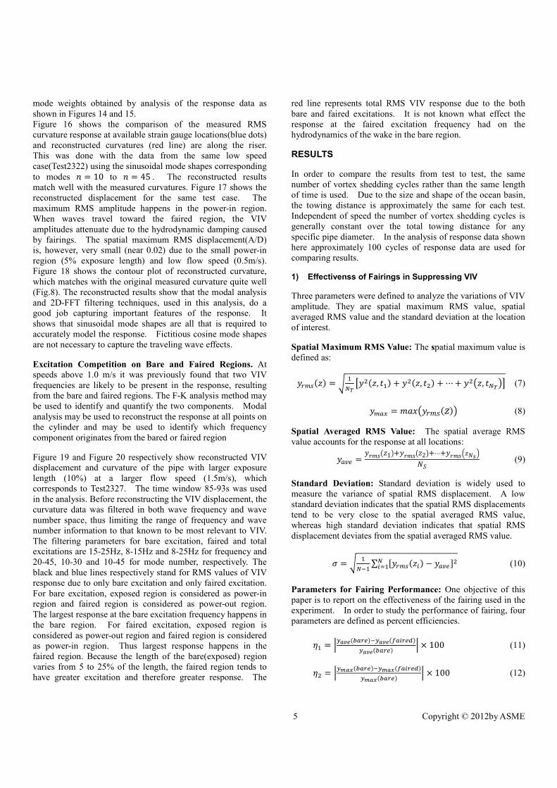
Spatial Maximum RMS Value: The spatial maximum value is

defined as:

;<+�&� = � �=> ?;��&, �� + ;��&, �� + ⋯ + ;�A&, �=>BC (7)

;�D = EFA;G 0�&�B (8)

Spatial Averaged RMS Value: The spatial average RMS

value accounts for the response at all locations:

;�HI = ;G 0A&1B+;G 0A&2B+⋯+;G 0J(K0LK, (9)

Standard Deviation: Standard deviation is widely used to

measure the variance of spatial RMS displacement. A low

standard deviation indicates that the spatial RMS displacements

tend to be very close to the spatial averaged RMS value,

whereas high standard deviation indicates that spatial RMS

displacement deviates from the spatial averaged RMS value.

M = � �=�� ∑ 3;<+�&O� − ;�HI5�=OP� (10)

Parameters for Fairing Performance: One objective of this

paper is to report on the effectiveness of the fairing used in the

experiment. In order to study the performance of fairing, four

parameters are defined as percent efficiencies.

Q� = RS�TU�V�<I��S�TU�W�O<IX�S�TU�V�<I� R × 100 (11)

Q� = RSZ�[�V�<I��SZ�[�W�O<IX�SZ�[�V�<I� R × 100 (12)


Q\ = R S�TU�V�<I ID]O^_^`ab�S�TU��c��d ID]O��Oce�R × 100 (13)

Qf = R SZ�[�V�<I ID]O^_^`ab�SZ�[��c��d ID]O��Oce�R × 100 (14)

There are only five runs for the fully faired pipe, there are

Test2302, Test2303, Test2304, Test2305 and Test2306

corresponding to flow speeds 0.5m/s, 1.20m/s, 1.32m/s,

1.44m/s and 1.56m/s, respectively. In order to compare VIV

response of fully faired pipe with that of bare pipe, some

approximations are made due to small number of velocities for

the fully faired pipe.

Approximation 1: When there is no flow speed for the fully

bared pipe corresponding to the flow speed of fully faired pipe,

a linear interpolation was made to find the amplitude at that

flow speed of fully faired pipe, expressions (11) and (12) are

used to study the efficiency of ribbon fairing.

Approximation 2: For the pipe covered with partial fairings,

the bare and faired excitations were separated according to

frequency content. Expressions (13) and (14) are used to

study the effectiveness of fairing in the suppression of VIV.

The efficiency of the fairing as a function of speed is shown in

Figure 21. The black squares were found using expressions

(11) or (13). The red dots were estimated using expressions

(12) or (14). Figure 21 shows that the efficiency of fairing

completely suppressed the VIV at flow speeds below 1m/s.

When the flow speed is above 1m/s, the efficiency of fairing

decreases to 20-30%.

2) Effect of Explosure Length on VIV

Figure 22 shows the effect of exposure length on VIV

amplitude. Markers represent flow speeds varying from 0.5m/s

to 2.5m/s. The bar represents the standard deviation of spatial

RMS values of displacement.

Bare Excitation: Figure 22 (a) and (b) show respectively the

spatial maximum and averaged RMS values of displacement

due to bare excitation associated with higher Strouhal number.

Both RMS values increase with exposure length, regardless of

flow speed. When the bare excitation was separated from the

total response, the pipe could be modeled as the power-in

region (same as the exposed region) is in the middle of pipe.

It was expected that with the increase of the power-in length,

more energy enters into the system, which leads to the increase

of VIV amplitude.

Faired Excitation: Figure 22 (c) and (d) show respectively the

spatial maximum and averaged RMS values of displacement

due to faired excitation associated with lower Strouhal number.

The test of the pipe with wrapping ribbon fairings was added at

the last minute as an extra test of opportunity. There was not

time or funding to make up or order airfoil shaped fairings.

These ribbon fairing are inexpensive and readily available, but

had unknown performance in suppressing VIV. From Figure

22 (c) and (d), the fairings wholly suppressed the VIV response

for lower flow speeds (0.5m/s and 0.75m/s). For higher flow

speeds, however, the fairing allowed VIV excitation. More

generally, RMS values decreased with increased length of the

bare region (decrease of the faired region). When the

excitation in the faired region was separated from the total

response, the exposed region could be considered as power-out

region and the faired region could be modeled as power-in

region. It was expected that with the increase of the exposure

length, the power-out region increased and the power-in region

decreased, thus accompanied by less energy entering into the

system, which leads to the decrease of VIV amplitude.

CONCLUSIONS

The primary contribution of this work is that it systematically

studies the effect of exposure length on VIV of flexible

cylinders with a bare section in the middle.

Summary observations and preliminary conclusions from the

VIV analysis of the flexible cylinder with symmetric fairings

installed at both sides of the pipe include:

1. The VIV response is dominating by traveling waves

for partially faired pipe.

2. Waves periodically changing direction was commonly

observed for low speed cases, and occasionally

observed at high flow speeds.

3. The flexible ribbon fairings were effective at

suppressing VIV at speeds below 1 m/s. Above 1m/s,

the fairing still could suppress to 10-30% of typical

VIV amplitudes.

4. The excitation on the bare and faired regions could be

identified by frequency, because the faired region

exhibited a much lower Strouhal number.

5. The response due to excitation on the bare region

increases with exposure length.

ACKNOWLEDGMENTS

The authors gratefully acknowledge Deepstar and the SHEAR7

JIP members (BP, Chevron, ExxonMobil, Petrobras, Shell,

Statoil & Technip) for supporting this research. And especially

SHELL Exploration and Production for providing the data. We

also thank Mr.Themistocles L.Resvanis for valuable

discussions.

NOMENCLATURE

1D FFT One dimensional Fast Fourier

Transform

2D FFT Two dimensional Fast Fourier

Transform

c The phase velocity

/ Hydrodynamic diameter


�� Time function

��&, �� Time and space function

�+� Vortex shedding frequency

�� The 1D FFT of ��

��, �� The 2D FFT of ��z, t�

� − g Frequency-Wavenumber

IFFT Inverse Fast Fourier Transform

� Wave number

hOe Exposure length

Mass per unit length

� Added mass

2 Mode number or sine term

Ki Number of sample in space

K� Number of sample in time

jk, Root mean square

,� Strouhal number

� Tension

- Flow speed

� Wave frequency in rad/s

;�&, �� VIV time series displacement

;�HI Spatial averaged RMS value of

;<+�&�

;�HI�lEG�� Spatial averaged RMS

displacements for fully bared pipe

;�HI�lEG� �F�1�E�1m2� Spatial averaged RMS displacement

due to bare excitation

;�HI��E1G�� Spatial averaged RMS

displacements for fully faired pipe

;�HI��m�En �F�1�E�1m2� Spatial averaged RMS

displacements due to total excitation

;�D Spatial maximum RMS value of

;<+�&�

;�D�lEG�� Spatial maximum RMS

displacements for fully bared pipe

;�D�lEG� �F�1�E�1m2� Spatial maximum RMS

displacements due to bare excitation

;�D��E1G�� Spatial maximum RMS

displacements for fully faired pipe

;�D��m�En �F�1�E�1m2� Spatial averaged RMS

displacements due to total excitation

;<+�&� Root mean square of ;�z, t�

! Delta function

M Standard deviation of ;<+�&�

Q� Parameter 1 of fairing performance

Q� Parameter 2 of fairing performance

Q\ Parameter 3 of fairing performance

Qf Parameter 4 of fairing performance

References [1] Vikas Gopal Jhingran(2008). Drag Amplification and

Fatigue Damage in Vortex-Induced Vibrations [D]. Ocean

Engineering, Massachusetts Institute of Technology,

Boston, USA.

[2] Don W.Allen and Dean L. Henning(2008). Comparisons

of Various Fairing Geometries for Vortex Suppression at

High Reynolds Numbers. Offshore Technology Conference,

OTC 19377.

[3] H.Lie, K.E.Kaasen(2006). Modal analysis of

measurements from a large-scale VIV model test of a riser

in linearly sheared flow [J]. Journal of fluids and structures,

22(4), P:557-575.

[4] Vivek Jaiswal(2009). Effect of Traveling Waves on Vortex-

Induced Vibration of Long Flexible Cylinders[D]. Ocean

Engineering, Massachusetts Institute of Technology,

Boston, USA.

[5] Harish Mukundan (2008). Vortex-Induced Vibration of

Marine Risers: Motion and Force reconstruction from field

and experimental data [D]. Ocean Engineering,

Massachusetts Institute of Technology, Boston, USA.

[6] S.I.McNeill and P.Agarwal (2011). Efficient Modal

Decomposition and Reconstruction of Riser Response due

to VIV. OMAE2011-49469.

[7] MARINTEK(2011). Shell Riser VIV Tests Main Report.

Main report No.580233.00.01. Norwegian Marine

Technology Research Institute.

[8] R.B.Campbell and J. K. Vandiver (1980). "The

Determination of Modal Damping Ratios from Maximum

Entropy Spectral Estimates", with R. B. Campbell,

Proceedings of the 1980 Offshore Technology Conference,

Houston, May 1980; also ASME Journal of Dynamic

Systems and Control, Vol. 104, March 1982.


APPENDIX

Fig.1: Configuration of the pipe with fairings. The exposed region (Bare region) was always in the middle of the pipe and the fairings were installed symmetrically towards both ends of the pipe.

Figure 2: Small pipe covered with wrapping ribbon fairings

Figure 3 The spatial extension of measured data. The red circles are the ends of the pipe; here they are also considered as four additional sensors with zero displacement in order to increase the resolution in space. The solid blue squares are measured data for 52 strain gauges. The sinusoidal response at one specific time is assumed. The orange crosses represent the extended data. In the left extended space, the extended data are symmetric about point (0, 0) with the measured data for any point in time. In the right extended space, the extended data are symmetric about point (1, 0) with the measured data for any point in time.

-1 -0.8 -0.6 -0.4 -0.2 0 0.2 0.4 0.6 0.8 1 1.2 1.4 1.6 1.8 2-1

-0.5

0

0.5

1

Extended data

The length of pipe

Extended Space Extended Space

Measured data

Original Space

Boundary condition as

additional sensor

b=1/2+Lin/2 a=1/2-Lin/2

Bare

Lin

Fairings

Z=0 Z=1

Fairings


Figure 4: Dispersion relation plot only in the first quadrant with 2D FFT to all curvatures for Test 2322. Test 2322 corresponds to 5% exposure length in the middle of the pipe under uniform flow 0.5m/s. The time section 66s to 71s was used. The color repents the Fourier coefficients of curvatures in dB. Red is the strongest and blue the weakest.

Figure 5: Filtered dispersion relation plot in all quadrants with 2D FFT to all curvatures for Test 2322. The filtered

parameters are 5-10Hz for wave frequency �o� and 10-45 for mode number corresponding to 0.83-3.72 for wave number�p�. 2D IFFT of circled peaks in the first and third quadrants are waves traveling from right to left or from top to bottom, while 2D IFFT of squared peaks in the second and fourth quadrants are waves traveling from left to right or from bottom to top.

Figure 6: Volumetric slice plots for dispersion relation with 2D FFT to all curvatures for all test cases with 5% exposure length in the middle of pipe. In order to display all 2D FFT plots in one figure. A 5 second time window is used. The slices from lower flow speed to higher flow speed correspond to the Test2322, Test2321, Test2318, Test2319 and Test2320, respectively. The corresponding time sections are 66-71s ,48-53s, 33-38s, 28-33s and 24-29s. The black arrow from lower flow speed to higher flow speed represents the bare excitation at a higher frequency and the blue arrow from lower flow speed to higher flow speed represents the faired excitation at a lower frequency.

Wave number

Frequency(Hz)

Test2322:Filtered Dispersion Relation

-4 -3 -2 -1 0 1 2 3 4-14

-12

-10

-8

-6

-4

-2

0

2

4

6

8

10

12

14

-50-45-40-35-30-25-20-15-10 -5 0 5 10 15 20 25 30 35 40 45 50

Mode Number

1st Quadrant 2nd Quadrant

3rd Quadrant 4th Quadrant

1st Quadrant

Lower frequency due to faired excitation

Higher frequency due to bare excitation


Figure 7: The frequency contents from fairing and barewere separated. Dominate peaks are plotted against flowspeed for uniform flow. St for bare excitation is about 0.143 and for fairing excitation is about 0.088.

Figure 8 Contour plot of curvatures filtered by 2D FFT. The

filtered parameters are 5-10Hz for wave frequency �q� and 10-45 for mode number corresponding to 0.83-3.72 for wave number�r�.

Figure 9: The traveling upward wave was separated from the total curvatures with 2D FFT. The 2D FFT was used to filter the original data. The filtering parameters are frequency from 5 to 10Hz and mode number from 10 to 45.

Figure 10: The traveling downward wave was separated from the total curvatures with 2D FFT. The 2D FFT was used to filter the original data. The filtering parameters are frequency from 5 to 10Hz and mode number from 10 to 45.

0 0.5 1 1.5 2 2.5 3 3.50

5

10

15

20

25

30

35

40

45

50

Flow Speed (m/s)

Response Frequency (Hz)

Bare

fbare

=0.143*U/D

Faired

ffaired

=0.088*U/D

Fairing excitation,St = 0.088

Bare excitation, St = 0.143


Figure 11: Time history of the 25

th strain gauge.

Figure 12 Spectrum of the 25

th strain gauge with time window

66.5-68.1s. The ‘pyulear’ function in the MATLAB was used

to get the spectrum plot. The peak frequency is 7.5Hz

Figure 13 Spectrum of the 25th strain gauge with time window

68.1-69.7s. The ‘pyulear’ function in the MATLAB was used

to get the spectrum plot. The peak frequency is 8.0Hz

Figure 14: RMS displacement mode weights using sine terms from s = tu to s = vw, almost 100 cycles corresponding to time window(66-90s) was used for reconstruction(Test 2322).

66 67 68 69 70 71

-1

-0.5

0

0.5

1

X: 66.46

Y: 0.2515

Curvature/M

ax

Time (s)

Test2322:25th Strain Gauge

X: 68.1

Y: 0.3723X: 69.72

Y: 0.3237

Envelope

Filtered Curvature

0 10 20 30 40 50 60 70 80 90 100-150

-100

-50

0

X: 7.498

Y: -7.932

Power/frequency (dB/Hz)

Frequency (Hz)


0 10 20 30 40 50 60 70 80 90 100-140

-120

-100

-80

-60

-40

-20

X: 8.002

Y: -21.91

Power/frequency (dB/Hz)

Frequency (Hz)


10 12 14 16 18 20 22 24 26 28 30 32 34 36 38 40 42 440

1

2

3

4

5

6x 10

-3

Mode number

RMS Displacement Mode W

eight/D

Sine term


Figure 15: RMS curvature mode weights using sine terms from s = tu to s = vw, almost 100 cycles corresponding to time window(66-90s) was used for reconstruction(Test 2322).

Figure 18 Contour plot of reconstructed curvatures with mode supersition. The sine terms are from 10 to 45.

Figure 16: Reconstructed RMS curvatures (red line) for Test2322 using the sine terms from n = 10 to n = 45, and 100 cycles (66-90s) was used for reconstruction.

Figure 17: Reconstructed RMS displacements (red line) for Test2322 using the sine terms from n = 10 to n = 45, and 100 cycles (66-90s) was used for reconstruction.

10 12 14 16 18 20 22 24 26 28 30 32 34 36 38 40 42 440

0.002

0.004

0.006

0.008

0.01

0.012

Mode number

RMS Curvature Mode W

eight(m

-1)

Sine term

0 1 2 3 4 5 6

x 10-4

0

0.1

0.2

0.3

0.4

0.5

0.6

0.7

0.8

0.9

1

Axial Position

RMS Curvature(1/m)

Test2322:Recon.Curv.

Reconstructed

Measurement

0 0.01 0.020

0.1

0.2

0.3

0.4

0.5

0.6

0.7

0.8

0.9

1

Axial Position

RMS Displacement/D

Test2322:Recon.Disp.

Reconstructed

Axial Position

Time(s)

Test2322:Reconstructed Curvature

66 67 68 69 70 710

0.1

0.2

0.3

0.4

0.5

0.6

0.7

0.8

0.9

1

-8

-6

-4

-2

0

2

4

6

8x 10

-4


Figure 19: Reconstructed RMS curvatures for 10% exposure length under uniform flow speed U=1.5m/s. The blue, black and red lines represent RMS values of curvature due to faired, bare and total excitation, respectively(Test 2327).

Figure 20: Reconstructed RMS displacements for 10% exposure length under uniform flow speed U=1.5m/s. The blue, black and red lines represent RMS values of curvature due to faired, bare and total excitation, respectively(Test 2327).

Fig.21: The efficiency of fairing in suppressing VIV. 100% means VIV is fully suppressed and 0% means VIV is never suppressed. The red dot stands for the efficiency of fairing estimated with the expression (16) and the black square stands for the efficiency of fairing estimated with the expression (15). The efficiencies of fairing at flow speed 0.75m/s, 1m/s and 1.5m/s were estimated with the expressions (17) and (18) for red dot and black square respectively.

0 0.005 0.01 0.0150

0.1

0.2

0.3

0.4

0.5

0.6

0.7

0.8

0.9

1

Axial Position

RMS Curvature(1/m)

10% Exposure Length-1.5m/s

Bare excitation

Fairing excitation

Both excitation

0 0.1 0.2 0.3 0.4 0.5 0.60

0.1

0.2

0.3

0.4

0.5

0.6

0.7

0.8

0.9

1

Axial Position

RMS Displacement/D

10% Exposure Length-1.5m/s

Bare excitation

Fairing excitation

Both excitation

0.4 0.5 0.6 0.7 0.8 0.9 1 1.1 1.2 1.3 1.4 1.5 1.60

10

20

30

40

50

60

70

80

90

100

Fairing Efficiency (%)

Flow Speed (m/s)

0.6 0.8 1 1.2 1.4 1.6 1.8

x 104Reynolds Number

Efficiency-Max.

Efficiency-Ave.

5% exposure length

10% exposure length


Figure 22: The effect of exposure length on VIV. (a) The spatial maximum RMS A/D with exposure length due to bare excitation. (b) The spatial averaged RMS A/D with exposure length due to bare excitation. (c) The spatial maximum RMS A/D with exposure length due to fairing excitation. (d) The spatial averaged RMS A/D with exposure length due to fairing excitation. The bar represents the standard deviation of spatial RMS displacement.

0 0.1 0.2 0.3 0.4 0.5 0.6 0.7 0.8 0.9 1 1.10

0.1

0.2

0.3

0.4

0.5

0.6

0.7

0.8

0.9

1

Exposure Length

Spatial Max RMS A/D

(a) Excitation at higher frequency (Bare section)

U=0.5

0.75

1.0

1.1

1.25

1.3

1.4

1.5

1.6

2.0

2.5

0 0.1 0.2 0.3 0.4 0.5 0.6 0.7 0.8 0.9 1 1.10

0.1

0.2

0.3

0.4

0.5

0.6

0.7

Exposure Length

Spatial Averaged RMS A/D

(b) Excitation at higher frequency (Bare section)

U=0.5

0.75

1.0

1.1

1.25

1.3

1.4

1.5

1.6

2.0

2.5

0 0.1 0.2 0.3 0.4 0.5 0.6 0.7 0.8 0.9 1 1.10

0.1

0.2

0.3

0.4

0.5

0.6

0.7

0.8

0.9

1

Exposure Length

Spatial Max RMS A/D

(c) Excitation at lower frequency (Faired section)

U=0.5

1.0

1.2

1.25

1.3

1.44

1.5

1.56

2.0

2.5

0 0.1 0.2 0.3 0.4 0.5 0.6 0.7 0.8 0.9 1 1.10

0.1

0.2

0.3

0.4

0.5

0.6

0.7

Exposure Length

Spatial Averaged RMS A/D

(d) Excitation at lower frequency (Faired section)

U=0.5

1.0

1.2

1.25

1.3

1.44

1.5

1.56

2.0

2.5

the effect of exposure length on vortex induced …

Documents