The Edge --- Randomized The Edge --- Randomized Algorithms for Network MonitoringAlgorithms for Network Monitoring

George VargheseOct 14, 2009

Research motivation

The Internet in 1969 The Internet today

Problems Flexibility, speed, scalability

Overloads, attacks, failures

Measurement & control

Ad-hoc solutions suffice

Engineered solutions needed

This talk: using randomized algorithms in network chips for monitoring performance and security in routers

Focus on 3 Monitoring Problems

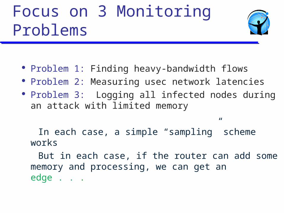
Problem 1: Finding heavy-bandwidth flows Problem 2: Measuring usec network latencies Problem 3: Logging all infected nodes during an

attack with limited memory

In each case, a simple “sampling” scheme works

But in each case, if the router can add some memory and processing, we can get an edge . . .

Get edge subject to constraints

Low memory: On-chip SRAM limited to around 32 Mbits. Not constant but is not scaling with number of concurrent conversations/packets

Small processing: For wire-speed at 40 Gbps, using 40 byte packets, have 8 nsec. Using 1 nsec SRAM, 8 memory accesses. Factor of 30 in parallelism buys 240 accesses.

Problem 1: Heavy-bandwidth users

Heavy-hitters: In a measurement interval, (e.g., 1 minute) measure the flows (e.g., sources) on a link that send more than a threshold T (say 1% of the traffic) on a link using memory M < < F, the number of flows

S1S6 S2 S5S2 S2

Source S2 is 30 percent of traffic sequence

Estan,Varghese, ACM TOCS 2003

Getting an Edge for heavy-hitters Sample: Keep a M size sample of packets.

Estimate heavy-hitter traffic from sample Sample and Hold: Sampled sources held in a

CAM of size M. All later packets counted Edge: Standard error of bandwidth estimate is

O(1/M) for S&H instead of O(1/sqrt(M)) Improvement: (Prabhakar et al): Periodically

remove “mice” from “elephant trap”

Problem 2: Fine-Grain Loss and Latency Measurement

(with Kompella, Levchenko, Snoeren)

SIGCOMM 2009, to appear

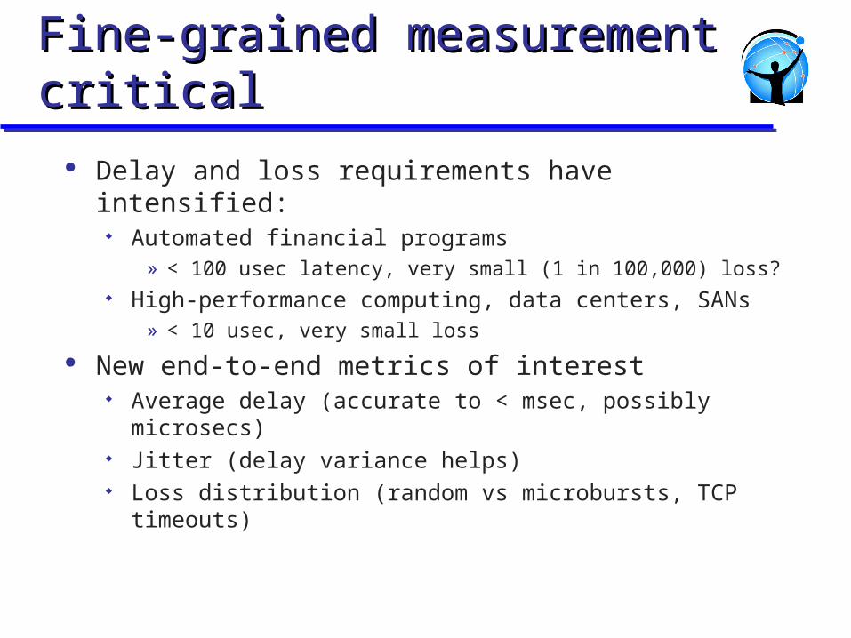
Fine-grained measurement criticalFine-grained measurement critical

Delay and loss requirements have intensified: Automated financial programs

» < 100 usec latency, very small (1 in 100,000) loss? High-performance computing, data centers, SANs

» < 10 usec, very small loss

New end-to-end metrics of interest Average delay (accurate to < msec, possibly microsecs) Jitter (delay variance helps) Loss distribution (random vs microbursts, TCP timeouts)

Existing router infrastructureExisting router infrastructure SNMP (simple aggregate packet counters)

Coarse throughput estimates not latency

NetFlow (packet samples) Need to coordinate samples for latency. Coarse

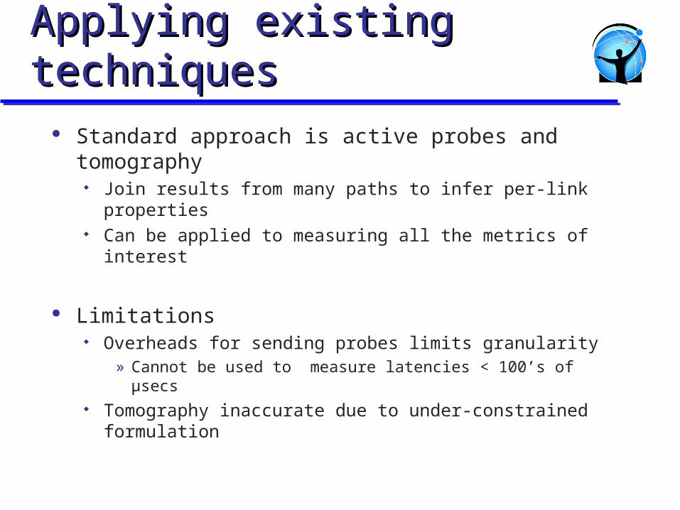
Applying existing techniquesApplying existing techniques Standard approach is active probes and tomography

Join results from many paths to infer per-link properties Can be applied to measuring all the metrics of interest

Limitations Overheads for sending probes limits granularity

» Cannot be used to measure latencies < 100’s of μsecs Tomography inaccurate due to under-constrained formulation

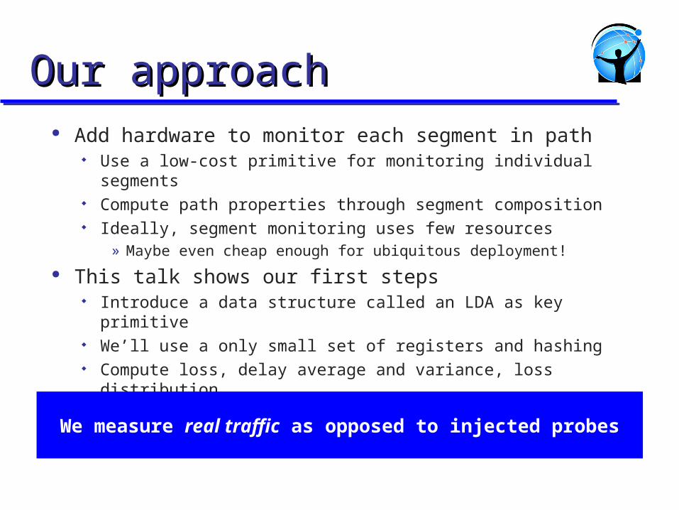
Add hardware to monitor each segment in path Use a low-cost primitive for monitoring individual segments Compute path properties through segment composition Ideally, segment monitoring uses few resources

» Maybe even cheap enough for ubiquitous deployment!

This talk shows our first steps Introduce a data structure called an LDA as key primitive We’ll use a only small set of registers and hashing Compute loss, delay average and variance, loss distribution

Our approachOur approach

We measure real traffic as opposed to injected probes

Model

Why simple data structures do not work

LDA for average delay and variance

Outline Outline

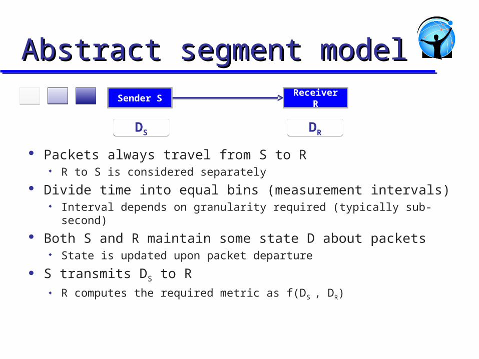
Packets always travel from S to R R to S is considered separately

Divide time into equal bins (measurement intervals) Interval depends on granularity required (typically sub-second)

Both S and R maintain some state D about packets State is updated upon packet departure

S transmits DS to R R computes the required metric as f(DS , DR)

Sender S Receiver R

DSDS DR

DR

Abstract segment modelAbstract segment model

Assumption 1: FIFO link between sender and receiver Assumption 2: Fine-grained per-segment time synchronization

Using IEEE 1588 protocol, for example Assumption 3: Link susceptible to loss as well as variable delay Assumption 4: A little bit of hardware can be put in the routers

You may have objections, we will address common ones later

Sender S Receiver R

AssumptionsAssumptions

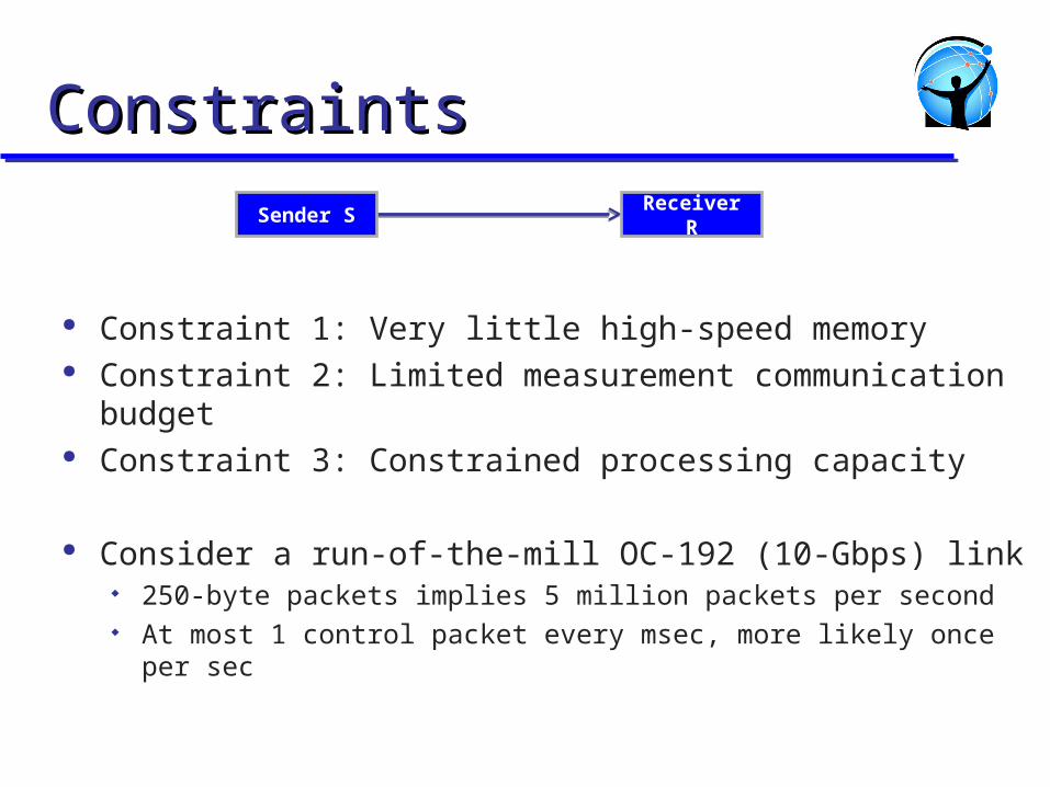
Constraint 1: Very little high-speed memory Constraint 2: Limited measurement communication budget Constraint 3: Constrained processing capacity

Consider a run-of-the-mill OC-192 (10-Gbps) link 250-byte packets implies 5 million packets per second At most 1 control packet every msec, more likely once per sec

Sender S Receiver R

ConstraintsConstraints

Store a packet counter at S and R. S sends the counter value to R periodically R computes loss by subtracting its counter value from

S’s counter

Sender S Receiver R

countercounter

1 123 2 Loss = 3 – 2 = 1

Computing lossComputing loss

Sender S

A naïve first cut: timestamps Store timestamps for each packet at sender, receiver After every cycle, sender sends the packet timestamps to the

receiver Receiver computes individual delays, and computes average 5M packets require ~ 25,000 packets (200 labels per packet)

1010

1212

1515

2323

2626

3535

Sender S Receiver R

1313

1414

2020

47/3 = 15.7Avg delay

Computing delay (naïve)Computing delay (naïve)

Extremely high communication and storage costs

(Slightly) better approach: sampling Store timestamps for only sampled packets at sender, receiver

1 in 100 sampling means ~ 250 packets

1010

1515

2323

3535

Sender S Receiver R

1313

2020

33/2 = 16.5Avg delay

Computing delay (sampled)Computing delay (sampled)

Less expensive, but we can get an edge . . .

Observation: Aggregation can reduce cost Store sum of the timestamps at S & R After every cycle, S sends its sum CS to R

R computes average delay as (CS – CR) / N Only one counter and one packet to send

Sender S Receiver R

84-37/3 = 15.7Avg delay

counter

10+12+15 23+26+35

Delay with no packet lossDelay with no packet loss

counter

Works great, if packets were never lost…

Consider two packets, first sent at T/2 and lost. Second sent at T, received at T. Receiver gets D = T/4

Lost packets can cause Error = O(T) where T is the size of the measurement interval

Failed quick fix: Bloom filter will not work Always a finite false positive probability

Delay in the presence of lossDelay in the presence of loss

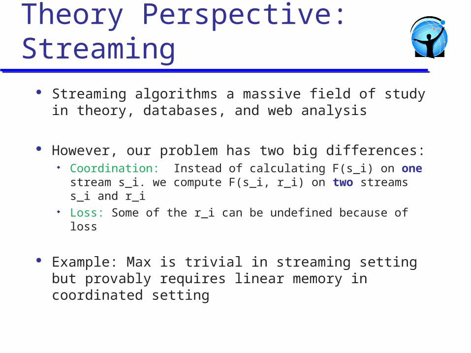
Theory Perspective: Streaming Streaming algorithms a massive field of study in

theory, databases, and web analysis

However, our problem has two big differences: Coordination: Instead of calculating F(s_i) on one stream s_i.

we compute F(s_i, r_i) on two streams s_i and r_i Loss: Some of the r_i can be undefined because of loss

Example: Max is trivial in streaming setting but provably requires linear memory in coordinated setting

(Much) better idea: Spread loss across several buckets Discard buckets with lost packets

Lossy Difference Aggregator (LDA) Hash table with packet count and timestamp sum

Sender S Receiver R

1010

1212

1515

1717

2323

2626 3939

+

+ +

2323

6565

11

22

2525

2929

22

22

00

3636

00

22- =

36/2= 18

Delay in the presence of lossDelay in the presence of loss

Sender S

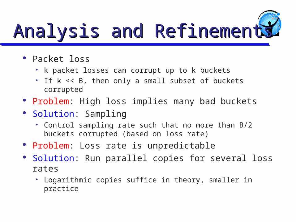
Packet loss k packet losses can corrupt up to k buckets If k << B, then only a small subset of buckets corrupted

Problem: High loss implies many bad buckets Solution: Sampling

Control sampling rate such that no more than B/2 buckets corrupted (based on loss rate)

Problem: Loss rate is unpredictable Solution: Run parallel copies for several loss rates

Logarithmic copies suffice in theory, smaller in practice

Analysis and RefinementsAnalysis and Refinements

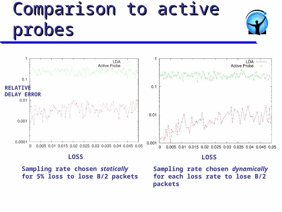
Sampling rate chosen statically for 5% loss to lose B/2 packets

Comparison to active probesComparison to active probes

RELATIVEDELAY ERROR

Sampling rate chosen dynamically for each loss rate to lose B/2 packets

LOSS LOSS

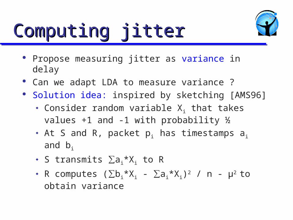
Propose measuring jitter as variance in delay Can we adapt LDA to measure variance ? Solution idea: inspired by sketching [AMS96]

Consider random variable Xi that takes values +1 and -1 with probability ½

At S and R, packet pi has timestamps ai and bi

S transmits ∑ai*Xi to R

R computes (∑bi*Xi - ∑ai*Xi)2 / n - µ2 to obtain variance

Computing jitterComputing jitter

E[( bi X i ai X i)2]

E[( i X i)2]

E[ i2 X i

2 2 i j X iX j ]

i2 E[X i

2] 2 i j E[X iX j ] i

2 =1 =0

Why this works (AMS 96)Why this works (AMS 96)

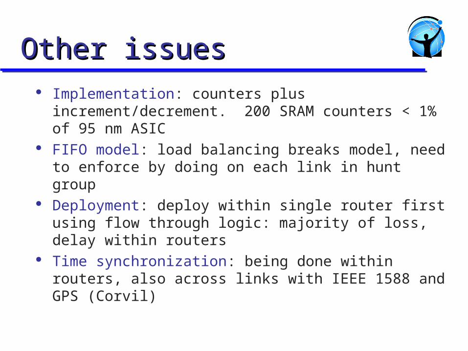
Implementation: counters plus increment/decrement. 200 SRAM counters < 1% of 95 nm ASIC

FIFO model: load balancing breaks model, need to enforce by doing on each link in hunt group

Deployment: deploy within single router first using flow through logic: majority of loss, delay within routers

Time synchronization: being done within routers, also across links with IEEE 1588 and GPS (Corvil)

Other issuesOther issues

With rise in modern trading and video applications, fine grained latency is important. Active probes cannot provide latencies down to microseconds

Proposed LDAs for performance monitoring as a new synopsis data structure

Simple to implement and deploy ubiquitously Capable of measuring average delay, variance, loss

and possibly detecting microbursts Edge is N samples (1 million) versus M samples

(1000) for no-error case. Reduces error by 300.

Summary of Problem 2Summary of Problem 2

Carousel --- Scalable and (nearly) Carousel --- Scalable and (nearly) complete collection of Information complete collection of Information

Terry Lam(with M. Mitzenmacher and G. Varghese, NSDI 2009)

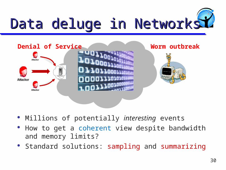
Data deluge in NetworksData deluge in Networks

Millions of potentially interesting events How to get a coherent view despite bandwidth and

memory limits? Standard solutions: sampling and summarizing

30

Denial of Service Worm outbreak

What if you want complete collection?What if you want complete collection?

Need to collect infected stations for remediation Other examples of complete collection:

List all IPv6 stations List all MAC addresses in a LAN

31

Example: worm outbreak Example: worm outbreak

32

SlammerWitty…

signatures

Intrusion Detection System (IDS)

Slammer A Witty BSlammer C

A B C

Management Station

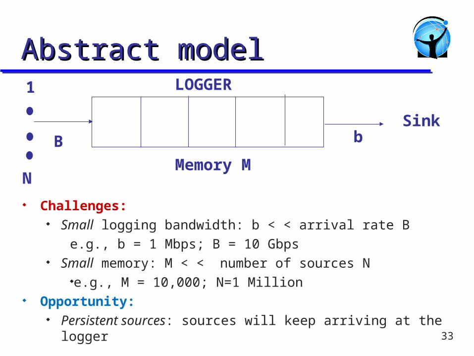
Abstract modelAbstract model

33

Challenges: Small logging bandwidth: b < < arrival rate B

e.g., b = 1 Mbps; B = 10 Gbps Small memory: M < < number of sources N

e.g., M = 10,000; N=1 Million Opportunity:

Persistent sources: sources will keep arriving at the logger

Sink

1

NMemory M

B b

LOGGER

Our resultsOur results

Carousel: new scheme, with minimal memory can log almost all sources in close to optimal time (N/b)

Standard approach is much worse ln(N) times worse in an optimistic random model Adding a Bloom filter does not help Infinitely worse in a deterministic adversarial model

34

Why the logging problem is Why the logging problem is hardhard

35

IDS

memory

sink

Sources 2 and 3 are never collected, 1 is logged many times. In general, some sources are always missed

2 34 141

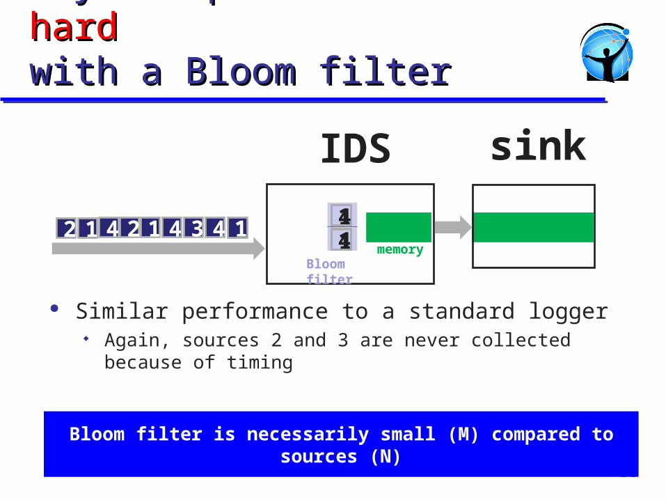
Why the problem is still Why the problem is still hardhardwith a Bloom filterwith a Bloom filter

36

Bloom filter is necessarily small (M) compared to sources (N)

Similar performance to a standard logger Again, sources 2 and 3 are never collected because of timing

IDS

memory

sink

Bloom filter

142 341 4 1412 14

Congestion Control for Logging? Random dropping leads to congestion collapse Standard solution: closed loop congestion (TCP) and

admission control: but needs cooperative sources What can a poor resource do to protect itself

unilaterally without cooperation from senders? Our approach: Randomized Admission Control.

Break sources into random groups and “admit” one group at a time for logging

Our solution: CarouselOur solution: Carousel

38

IDS

memoryBloom filter

sink

133 3424 121

Carousel

3 3424 121

Hash to color the sources say red and blue

Rotating the CarouselRotating the Carousel

39

IDS

memoryBloom filter

sink

Carousel

13422 3 43 1 134

Change color!

How many colors in Carousel?How many colors in Carousel?

40

IDS

memoryBloom filter

sink

13

Carousel

Bloom filter fullIncrease Carousel colors

42 341 5 174678 8 148

Summary of Carousel algorithmSummary of Carousel algorithm Partition

Hk(X): lower k bits of H(S), a hash function of a source S

Divide the population into partitions with same hash value

Iterate T = M / b (available memory divided by logging bandwidth) Each phase last T seconds, corresponds a distinct hash value Bloom filter weeds out duplicates within a phase

Monitor Increase or decrease k to control the partition size

41

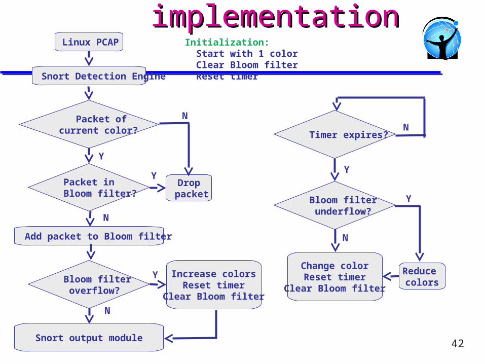
Snort implementationSnort implementation

42

Linux PCAP

Snort Detection Engine

Packet ofcurrent color?

Packet in Bloom filter?

Add packet to Bloom filter

Bloom filter overflow?

Snort output module

Increase colorsReset timer

Clear Bloom filter

Bloom filter underflow?

Change colorReset timer

Clear Bloom filter

Timer expires?

Drop packet

N

Y

N

Y

Y

Y

N

Reduce colors

N

Y

N

Initialization: Start with 1 color Clear Bloom filter Reset timer

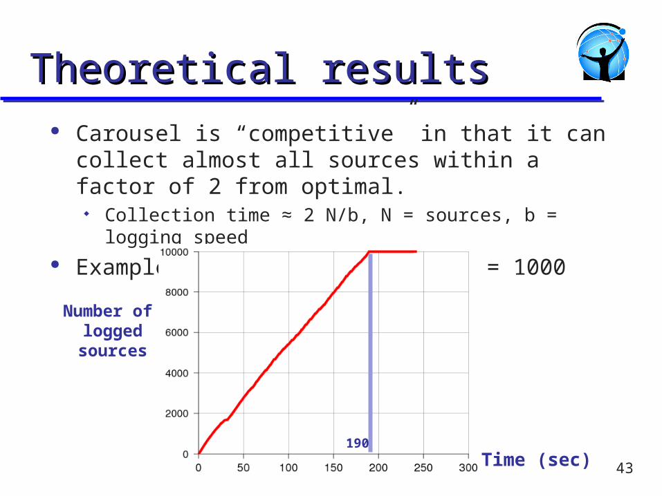
Theoretical resultsTheoretical results Carousel is “competitive” in that it can collect almost

all sources within a factor of 2 from optimal. Collection time ≈ 2 N/b, N = sources, b = logging speed

Example: N = 10,000 M = 500, b = 1000

43

Number of loggedsources

Time (sec)190

Simulated worm outbreaksSimulated worm outbreaks

N = 10,000; M = 500; b = 100 items/sec Logistic model of worm growth

44

Time (sec)

Number of loggedsources

400 39002100

Carousel nearly ten times faster than naïve collector

Snort Experimental Setup

Scaled down from real traffic: 10,000 sources, buffer of 500, input rate =100 Mbps, logging rate = 1 Mbps

Two cases: source S picked randomly on each packet or periodically (1,2,3 . . 10,000, 1, 2, 3, . . )

Snort resultsSnort results

46

Time (sec) Time (sec)

(a) Random traffic pattern (b) Periodic traffic pattern

180 500 18000

3 times faster with random and 100 times faster with periodic

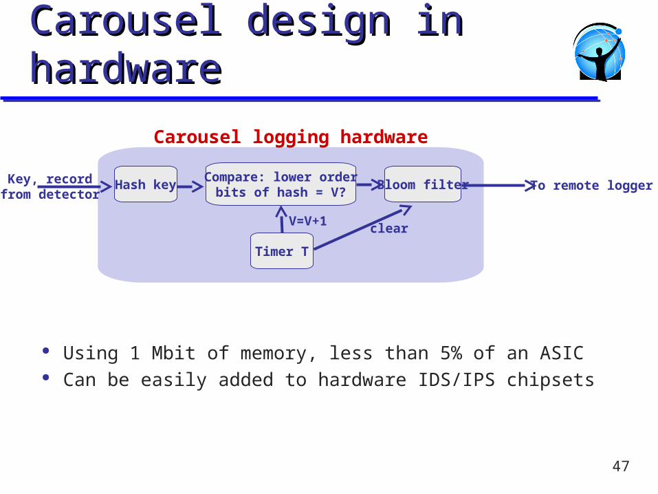
Carousel design in hardwareCarousel design in hardware

Using 1 Mbit of memory, less than 5% of an ASIC Can be easily added to hardware IDS/IPS chipsets

47

Hash keyCompare: lower order

bits of hash = V?Bloom filter

Timer T

V=V+1clear

Carousel logging hardware

Key, recordfrom detector

To remote logger

Related workRelated work High speed implementations of IPS devices

Fast reassembly, normalization and regular expression No prior work on scalable logging

Alto file system: dynamic and random partitioning Fits big files into small memory to rebuild file index after crash Memory is only scarce resource Carousel handles both limited memory and logging speed Carousel has a rigorous competitive analysis

48

Limitations of CarouselLimitations of Carousel Carousel is probabilistic: sources can be missed with

low probability mitigate by changing hash function on each Carousel cycle.

Carousel relies on a “persistent source assumption” Does not guarantee logging of “one-time” events

Carousel does not prevent duplicates at the sink but has fast collection time even in an adversarial model.

49

ConclusionsConclusions Carousel is a scalable logger that

Collects nearly all persistent sources in nearly optimal time Is easy to implement in hardware and software Is a form of randomized admission control

Applicable to a wide range of monitoring tasks with: High line speed, low memory, and small logging speed And where sources are persistent

50

Edge can be an order of magnitude

RAC is factor of 2 off from optimal to log all sources versus ln N/M off for naïve.

For N = 1 million and M small, edge is close to 14 for random arrivals; infinite for worst-case

LDA offers N samples versus M samples for naïve ‘ For N = 1 million, M = 10,000, edge is close to 10

Sample and Hold offers O(1/M) standard error versus O(1/sqrt(M)) for naïve

For M = 10,000, edge in standard error is 100

Related Work

LDA: Streaming Algorithms: less work on 2-party streaming

algorithms between a sender and receiver Network tomography: joins the result of black box

measurements to infer link delays and losses RAC:

Random partitions a common idea. We apply to admission control and add cycling through partitions

Alto Scavenger “discards information for half the files” if disk full

Summary

Monitoring networks for performance problems and security at high speeds is important but hard

Randomized streaming algorithms can offer cheaper (in gates) solutions at high speeds.

Described two simple randomized algorithms LDA: Aggregate by summing, hash to withstand

loss RAC: Randomly partition input into small enough

sets. Cycle through sets for fairness.

In conclusion . . .

The Edge

Venky: some renewal assumptions needed. Can estimate renewal times by sampling someone in each sampling group (real ID) and storing arrival timestamp and seeing how long it takes to return. Keep a few samples each time. Why sample. Why not take first few. May have bias/ Have two classes. Slow and fast. In that case sample a few randomly in class when a new one comes in (1 in M probability). Then watch him across intervals. Start with large interval and reduce. Too conservative T will lead to large overstimates N/M * T, if T is twice as large as real renewal time, then time is doubled over optimal

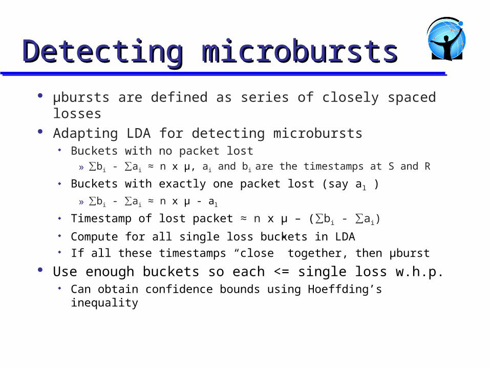
μbursts are defined as series of closely spaced losses Adapting LDA for detecting microbursts

Buckets with no packet lost» ∑bi - ∑ai ≈ n x μ, ai and bi are the timestamps at S and R

Buckets with exactly one packet lost (say al )

» ∑bi - ∑ai ≈ n x μ - al

Timestamp of lost packet ≈ n x μ – (∑bi - ∑ai) Compute for all single loss buckets in LDA If all these timestamps “close” together, then μburst

Use enough buckets so each <= single loss w.h.p. Can obtain confidence bounds using Hoeffding’s inequality

Detecting microburstsDetecting microbursts