THE ECONOMIC LEGACY OF EXPULSION:

LESSONS FROM POSTWAR CZECHOSLOVAKIA

Short title: The Economic Legacy of Expulsion

Patrick A. Testa∗

November 13, 2020

Abstract

This paper examines the long-run effects of forced migration on economic developmentin the origin economy, using Czechoslovakia’s expulsion of 3 million Germans afterWWII. For identification, I use the discontinuity in ethnic composition at the borderof the Sudetenland region where Germans lived. Germans had similar characteristics toCzechs, bypassing factors driving effects in other cases of forced migration, such as dif-ferences in human capital. The expulsion produced persistent disparities in populationdensity, sector composition, and educational attainment. I trace effects to selective ini-tial resettlements and capital extraction following the expulsion, culminating in urbandecay and human capital decline.

JEL codes: D74, N34, N94, R12, O15, I25Key words: Expulsion; forced migration; local development; postwar; nationalism

∗Department of Economics, 6823 St. Charles Avenue, Tulane University, New Orleans, LA 70118, UnitedStates of America. Email: ptesta@tulane.edu. Phone: +1 (507) 261-7728. I am grateful to the editor,Ekaterina Zhuravskaya, and three anonymous referees; to Dan Bogart, Jean-Paul Carvalho, and StergiosSkaperdas for their invaluable guidance; to Vellore Arthi, Jan Brueckner, Felipe Valencia Caicedo, GregClark, Kara Dimitruk, Kerice Doten-Snitker, James Fenske, Andy Ferrara, Price Fishback, Matt Freedman,Taylor Jaworski, Remi Jedwab, Noel Johnson, Ethan Kaplan, Dan Keniston, Erik Kimbrough, Alex Klein,Mark Koyama, Elie Murard, John Nye, Martha Olney, Elias Papaioannou, Santiago Perez, Debraj Ray,Gary Richardson, Jean-Laurent Rosenthal, Jared Rubin, Albert Sole-Olle, John Wallis, and countless othersat Alberta, Chapman, GMU, LSU, Stanford, Tulane, UC Berkeley, UC Irvine, Utah, Warwick, the 2018ASREC Meeting, the 2018 EHA Meeting, and the 13th UEA Meeting for useful comments; and to PavelHajek at the Czech Statistical Office, Jana Jıchova and Krystof Krotil for help with data collection. I amalso deeply indebted to Jordi Martı-Henneberg and his team at HGISe group (http://europa.udl.cat) forproviding me with rail GIS data. Thanks to the School of Social Sciences at UC Irvine and the Institute forHumane Studies for financial support. All errors are my own.

1 Introduction

Between 1945 and 1947, 3 million Germans were expelled from Czechoslovakia, in one of the

largest waves of forced migration in history. Yet this event was hardly unique. Countless

others, including millions of Jews, Greeks, and Turks, were likewise uprooted during the 20th

century in the process of nation-building, while civil and ethnic conflict have more recently

driven large-scale population outflows in places like Uganda, Bosnia, Syria, and Myanmar.

A large literature has documented the impact of such events, both on forced migrants, who

often experience continued persecution abroad as refugees, and on their host economies (Ruiz

and Vargas-Silva, 2013; Becker et al, 2020).

What, however, becomes of the places left behind? Comparably little work has been done

to understand how forced migration affects the economic development of places at origin,

i.e. from which the displacement occurred. In this paper, I examine such effects over the

long-run, using Czechoslovakia’s expulsion of 3 million Germans after WWII. This event

has several features which turn out to be well-suited for identifying the effects of a forced

migration event in ways that prior literature has not. Following the collapse of Austria-

Hungary into nation-states in 1918, those identifying as German within the Czech lands

(i.e. the modern day Czech Republic) were concentrated in one region – the borderlands, or

Sudetenland – distinguished by a distinct ‘language border.’ Yet after centuries of coexistence

and common rule, during which language had held little economic or social significance

among the masses, Germans and Czechs were highly similar in terms of their economic and

cultural characteristics (Zahra, 2008). This language border was made formal in 1938 with

the Munich Agreement, which paved the way for Germany’s occupation of the Czech lands

and in turn Czechoslovakia’s expulsion of its German population in 1945.

My identification strategy exploits the discontinuity in regional exposure to the expul-

sion at this boundary to identify its relative impact on local economic development over

the long-run.1 To do this, I construct a new dataset of municipal- and district-level data

1Use of ethnic boundaries for empirical identification follows a recent literature, including Michalopoulos

1

spanning nine decades. Using directories of Czech villages from during the war, I divide

the Czech lands into a borderlands region where Germans lived prior to the expulsion and

an interior region in which they largely did not. I then examine economic outcomes in the

borderlands, relative to interior areas nearby. To the extent that regions were historically

similar at the boundary prior to the expulsion, differences at the boundary thereafter re-

veal the expulsion’s relative effects.2 The prospect of similar treated and control areas also

presents a unique opportunity to examine the mechanisms through which forced migration

affects regional development. In other cases of forced migration, differences in factors such as

skill composition tend to distinguish displaced populations, driving effects (Acemoglu et al,

2011; Chaney and Hornbeck, 2016). In contrast, the effects of forced migration in this setting

are a priori ambiguous. Namely, it is not clear whether depopulation will be followed by

convergence (Davis and Weinstein, 2002; 2008), with migration restoring pre-existing spatial

patterns of economic activity at the boundary, or by a permanent redistribution of activity

to unaffected regions (Bosker et al, 2007; Bleakley and Lin, 2012), given the large negative

shock to borderland agglomerations. This paper seeks to answer this question and, if it is

the latter, chart the precise channels driving persistence.

I begin by combining historical evidence and data on a large set of socioeconomic variables

from the interwar period to confirm that places with many Germans and nearby places with

few were otherwise highly similar prior to the expulsion on a number of relevant dimensions,

such as literacy, income, and sector composition. This is true even if one omits segments of

the language border around which the borderlands was more ethnically mixed.

Next, I document large disparities in economic performance today between municipalities

on either side of the old German language border. As of 2011, crossing into a borderland

municipality from a nearby interior municipality is associated in main specifications with

a decline in population density (↓ 36.6%); higher unemployment (↑ 26%); a lower share of

and Papaioannou (2013), Grosfeld et al (2013), Eugster et al (2017), and Moscona et al (2020).2Effects are best described as relative effects, which are likely smaller than the expulsion’s absolute effects,

due to migration and trade from the interior to the borderlands following the expulsion.

2

employment in skill-intensive sectors such as finance (↓ 26.2%) and healthcare (↓ 21.2%); and

a smaller share of the population with a college degree (↓ 22.2%). These findings are robust

to changes in assumptions regarding bandwidth, running polynomial, and fixed effects.

Lastly, studying a historical expulsion allows me to shed light on the precise channels

through which such differences emerged and persisted. Contrary to policymakers’ expecta-

tions that former-German areas could be fully and voluntarily resettled by Czechs from the

largely unaffected interior, I show that the expulsion was followed by a selective migratory

response. Settlers disproportionately migrated from interior areas nearby and were rural in

origin relative to their more urban destinations, with fewer workers arriving from skilled

sectors such as transportation and business relative to agriculture. I argue that this is con-

sistent with agglomeration spillovers keeping relatively urban workers concentrated in the

interior after the expulsion. At the same time, I document a large-scale removal of phys-

ical capital from former-German areas following the expulsion. I argue that this stemmed

not from WWII or the Soviet liberation of the Czech lands thereafter, but from an extrac-

tive environment engendered by the vacuum of property rights that followed the expulsion.

Together, these forces culminated in widespread urban decay, with many settlements perma-

nently abandoned, lowered population density, and a shift in sectoral composition toward

agriculture in former-German areas, as well as human capital inequalities between the re-

gions, with relatively lower levels of enrollment in advanced secondary, technical, and tertiary

schooling present in the borderlands as early as mid-1947. I also consider other factors such

as natural geography, central planning, market access, and Cold War geopolitics.

The borderlands’ decline was initially not intended by Czechoslovak policymakers, for

whom the region had great economic importance. Yet the expulsion of the Germans had a

persistent impact on the places in which they had once lived, relative to other places nearby.

These findings provide valuable new insight into the economic effects of forced migration.

While voluntary migration has been the subject of vast research and debate (Bell et al, 2013;

Abramitzky et al, 2014), migration occurring due to expulsion as well as war and natural

3

disaster is increasingly relevant, with the UN placing the number of forcibly displaced people

at 80 million worldwide.3 Moreover, forced migration is often followed by expropriation and

conflict. Hence, it may have effects that differ from those of voluntary migration.

This paper makes several contributions to the literature on forced migration. First,

whereas existing research has focused largely on the effects of forced migration events for

host countries (Hornung, 2014; Schumann, 2014; Johnson and Koyama, 2017; Braun et al,

2020) or on migrants themselves (Bauer et al, 2013; Becker et al, 2020), the findings here

provide new evidence that forced migration may affect regional development and contribute

to spatial inequality in the origin economy overseeing such displacement (Becker and Ferrara,

2019). This is most similar to Chaney and Hornbeck (2016), who find delayed convergence

following the Spanish expulsion of the Moriscos between former-Morisco and non-Morisco

districts. As in their paper, studying a politically-motivated expulsion has advantages for

identification here, as it is less likely to be associated with selection within the targeted

group or the direct destruction of physical capital, relative to war or natural disaster.4

Second, to my knowledge this paper contributes the first evidence that forced migration

can have persistent effects even when treated and control groups are highly similar – in

contrast to other settings, in which pre-existing differences in skill or other factors are key in

driving spatial disparities following treatment (Acemoglu et al, 2011; Chaney and Hornbeck,

2016).5 Studying this event thus has the potential to speak to a more general class of forced

migration events, in which such differences are not always present to impede convergence.

Nevertheless, the findings here at times mirror other settings.6 For instance, Acemoglu et al

(2011) find similarly persistent population effects. In contrast, Arbatli and Gokmen (2019)

document a positive legacy of historical Greek and Armenian human capital externalities in

3See the United Nations High Commissioner for Refugees (2019).4An estimated 7000 German civilians were murdered by Czechs during the expulsion, and each expellee

was allowed to take about 50 kg in property (Gerlach, 2017).5Also see Waldinger (2010), Akbulut-Yuksel and Yuksel (2015); and Pascali (2016).6Effects also mirror the literature on refugee and other migrant inflows, in which population increases

often generate agglomeration or other spillovers that persist over the long-run (Foged and Peri, 2016; Rochaet al, 2017; Droller, 2017; Murard and Sakalli, 2019; Sequeira et al, 2019; Peters, 2019).

4

Turkey a century after the expulsions of those relatively high-skilled groups.

A third contribution to the forced migration literature is in documenting the regional

economic impact of this significant forced migration event in history. That being said,

several working papers study other important aspects of this event, complementing the work

here. In particular, Semrad (2015) focuses on the host economies of Sudeten Germans and

finds that their arrival in Bavaria generated educational spillovers, while Guzi et al (2019)

examine the migratory tendencies of those who resettled the borderlands and find that their

settlements tend to be less permanent, stemming from less developed social capital.

Lastly, this paper speaks to broader questions in development and urban economics

regarding the importance of historical shocks for long-run development. Empirically, the

findings contrast with Davis and Weinstein (2002; 2008), who argue against the empirical

relevance of multiple equilibria in economic activity, showing on the contrary that relative

city sizes recovered quickly in Japan following the destructive bombings of WWII.7 Yet

whereas that shock left property rights and ownership largely intact in affected cities (Nunn,

2014), none displaced by the expulsion here were around to help restore prior economic

geography thereafter, leaving a vacuum of property rights in the interim. I argue that this

paved the way for large-scale capital extraction, at the expense of regional recovery. This

mirrors Ochsner (2017), who documents a persistent negative impact of Red Army pillaging

of capital after WWII. This potentially offers an alternative explanation for the differential

effects of population shocks as noted in Acemoglu et al (2011), who attribute the Holocaust’s

persistent effects in Russia to structural changes stemming from compositional differences

between expellees and non-expellees. Namely, the persistent effects of shocks may depend

on how they affect such fundamental factors as property rights, as in Ochsner (2017) as well

as Nunn (2008) and Feigenbaum et al (2019).8

7On multiple equilibria, see Redding et al (2011), Kline and Moretti (2014), Jedwab and Moradi (2016).8Property rights for instance may help re-coordinate activity post-shock. See Acemoglu et al (2002),

Hornbeck (2010), Tabellini (2010), Dell (2010), and Acemoglu and Dell (2010) on history, institutions, anddevelopment, and Maloney and Caicedo (2015), Jedwab et al (2019), Dell and Olken (2019), and Testa (2020)for prior work on how agglomeration economies and institutions may interact to shape spatial development.

5

2 Historical background

The origins of the ‘Sudeten’ Germans in the Czech borderlands can be traced to the 12th

century, when early Bohemian kings opened them up to immigration by German-speaking

artisans (de Zayas, 1989). They would pay taxes but trade relatively freely, diffusing their

language and culture in the process (Agnew, 2004).

After the Thirty Years’ War, the Czech lands underwent further ‘Germanization’ under

Habsburg rule. During this time, more German speakers moved into the borderlands, creat-

ing vast German language frontiers (Danek, 1995). Yet despite growing German hegemony

among the elite, German and Czech speakers coexisted peacefully at the local level, where

identity depended more on local kinships than on language (King, 2002; Tampke, 2003).

German industries attracted Czech speakers to German towns, creating bilingual economic

centres where intermarriage was not uncommon and language choice was situational (Ag-

new, 2004; Zahra, 2008). By the early 1800s, language was largely independent of economic,

cultural, or even genetic factors among the masses (King, 2002; Zahra, 2008).

The formation of a German ‘language border’

Though German and Czech speakers remained well-matched economically, a series of events

resulted in their increased segregation within the Czech lands during the following century.

From the late 1800s, nationalist activists worked to build exclusive societies by establishing

language-based social associations and lobbying for reforms that limited bilingual education

(Tampke, 2003; Judson, 2006; Zahra, 2008). These efforts often took on a geographic di-

mension. Because later Austrian censuses required citizens to select a single language of

daily use, German nationalists developed a visual of the borderlands as a distinctly German

region and aimed to ‘Germanize’ its mixed elements. Czech nationalists, in contrast, sought

to preserve the historic boundaries of the Lands of the Bohemian Crown (i.e. the modern day

Czech Republic) and built exclusively Czech-language institutions to combat Germanization

(Bryant, 2002; Zahra, 2008). As a result, much of activists’ efforts focused on the more

6

mixed areas where the borderlands met the Czech interior (Cornwall, 1994). And although

the masses remained largely indifferent to national identification, the late 19th century in-

deed saw greater language assimilation in these places, including declining German speaking

in interior areas (Agnew, 2004; Zahra, 2008).

The notion of the borderlands as a formal, German region was further legitimized in 1918

when it was included in official proposals for a new German-Austrian state (Agnew, 2004).

When the Allies instead backed Czech efforts to keep historic boundaries intact, the inclusion

of 3 million borderland German speakers as a minority group in the new Czechoslovak state

further unified them around a cohesive ‘Sudeten’ German identity (Gerlach, 2017). Mean-

while, Czechoslovak policymakers could now use the state to influence the ethnolinguistic

composition of the Czech lands. After 1918, a parent’s nationality as it appeared on the

census determined a child’s language of instruction, with minority-language schooling and

public services being provided only if a minority group exceeded 20% of the local population

(Zahra, 2008; Agnew, 2004). Coinciding with this, census officials could choose nationalities

for citizens based on ‘objective’ traits and punish failures to comply. In total, German pop-

ulation counts in mixed areas fell by 420,000 (Zahra, 2008). At least officially, over 90% of

German speakers in the Czech lands lived in the borderlands in 1930.

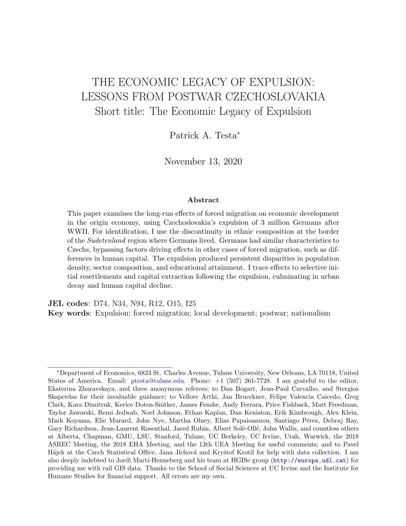
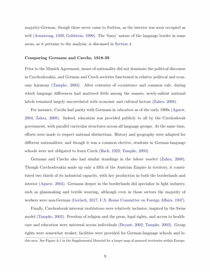
Though the interior was largely homogeneously Czech in official statistics after the 1921

census, parts of the borderlands remained quite mixed, and campaigns to influence the

German ‘language border’ as depicted in the first part of Figure 1 continued until its for-

malization with the Munich Agreement in 1938, which annexed all majority-German areas

to Nazi Germany.9 Parts of northeast Moravia even became minority-German in later years,

as Czechs-identifiers moved to some borderland cities (Cornwall, 1994). However, Hitler’s

proposals at Munich ignored this, successfully arguing for Germany’s annexation of border-

land villages that had been majority-German in 1910, with boundaries shown in the second

part of Figure 1.10 In fact, they also called for plebiscites in territories that had never been

9See Figure A.13 for the MAL directly overlaid on this map.10Note that Zaolzie in Cieszyn Silesia, a Polish-speaking area, was annexed by Poland in 1938. I exclude

7

(a) Germans in the Czech lands, pre-1945

(b) The Czech lands after the Munich Agreement

Figure 1: The German ‘language border’ and Munich Agreement boundaries. Notes: Sources for top map

are Winkler (1936), Wiskemann (1938), and Maier (2006). Bottom map shows the ‘Munich Agreement

line,’ constructed as described in Section 3.

8

majority-German, though these never came to fruition, as the interior was soon occupied as

well (Armstrong, 1939; Goldstein, 1999). The ‘fuzzy’ nature of the language border in some

areas, as it pertains to the analysis, is discussed in Section 4.

Comparing Germans and Czechs, 1918-39

Prior to the Munich Agreement, issues of nationality did not dominate the political discourse

in Czechoslovakia, and German and Czech societies functioned in relative political and econ-

omy harmony (Tampke, 2003). After centuries of coexistence and common rule, during

which language differences had mattered little among the masses, newly-salient national

labels remained largely uncorrelated with economic and cultural factors (Zahra, 2008).

For instance, Czechs had parity with Germans in education as of the early 1900s (Agnew,

2004; Zahra, 2008). Indeed, education was provided publicly to all by the Czechoslovak

government, with parallel curricular structures across all language groups. At the same time,

efforts were made to respect national distinctions. History and geography were adapted for

different nationalities, and though it was a common elective, students in German-language

schools were not obligated to learn Czech (Bach, 1923; Tampke, 2003).

Germans and Czechs also had similar standings in the labour market (Zahra, 2008).

Though Czechoslovakia made up only a fifth of the Austrian Empire in territory, it consti-

tuted two thirds of its industrial capacity, with key production in both the borderlands and

interior (Agnew, 2004). Germans deeper in the borderlands did specialize in light industry,

such as glassmaking and textile weaving, although even in those sectors the majority of

workers were non-German (Gerlach, 2017; U.S. House Committee on Foreign Affairs, 1947).

Finally, Czechoslovak interwar institutions were relatively inclusive, inspired by the Swiss

model (Tampke, 2003). Freedom of religion and the press, legal rights, and access to health-

care and education were universal across individuals (Bryant, 2002; Tampke, 2003). Group

rights were somewhat weaker; facilities were provided for German-language schools and le-

this area. See Figure A.1 in the Supplemental Material for a larger map of annexed territories within Europe.

9

gal activities, though only in areas in which Germans exceeded 20% of the population, and

Germans participated in parliamentary politics but were not guaranteed proportionate rep-

resentation (Tampke, 2003; Zahra, 2008).

Such calm was short-lived. During the Great Depression, economic anxiety amplified

German concerns about the Czechoslovak state. Export-heavy industries deep in the border-

lands experienced some of the highest unemployment in Czechoslovakia, and many Germans

blamed the Czechoslovak government. The separatist Sudeten German Party (SdP) was

founded in October of 1933, and although the popular German political parties remained

anti-separatist and coalesced with leading Czech parties on common issues in the 1920s, by

1938, 85% of Sudeten Germans supported the SdP (de Zayas, 1989; Glassheim, 2016).

Germany’s proximity to the borderlands made its invasion highly likely. In an attempt

to avoid war, Allied leaders signed the Munich Agreement, fully formalizing the Sudetenland

as a region. Meant to appease Germany, annexation severely weakened Czechoslovakia’s

military and industrial capacities (Agnew, 2004; Glassheim, 2016). Within a few months,

Germany had occupied the remainder of the Czech lands, sending its government into exile.

The expulsion of the Sudeten Germans

During the war, exiled Czechoslovak president Edvard Benes established the legal basis for

the expulsion of all Germans through several decrees. Thousands of ‘national committees’

were to be set up throughout the borderlands to manage the expulsion, including the con-

fiscation of German property without compensation and its allocation to incoming settlers.

When the war ended in 1945, Allied forces moved into the borderlands to liberate Czechoslo-

vakia, resulting in the first expulsions. It was not until June, however, that they would gain

momentum. By summer’s end, 800,000 Germans had been expelled. In August, following the

formal Allied approval of the expulsions at Potsdam, all remaining Germans were formally

stripped of their citizenship. Another 2.2 million Germans were expelled through mid-1947

(Gerlach, 2017). These transfers were more systematic in comparison to the earlier ‘wild

10

transfers.’ All borderland residents were suspected of being German. When in doubt, Ger-

man or Czechoslovak censuses could determine whether one should be expelled. This meant

that some Germans who had become Czechs by force prior to the war were not expelled,

while some non-Germans who had ‘switched’ to German following annexation were. For

others, having an ambiguous or mixed national identity meant being expelled, regardless of

census identification (Zahra, 2008; Spurny, 2013). Only a small number of Germans who

were Czech by marriage, could prove their loyalty to the state, or were deemed economi-

cally vital were allowed to stay. By 1950, 3 million Germans had been expelled, mainly to

the Western Zones of occupied Germany, along with almost a million to the East Zone and

142,000 to Austria, and only 165,000 Germans remained, of which most would be re-granted

citizenship (Cornwall, 1994; Odsun: Die Vertreibung der Sudetendeutschen, 1995).

The resettlement of the borderlands

The borderlands’ resettlement was of central importance to the Czechoslovak government,

which sought to maintain the region’s prewar output (Glassheim, 2016; Gerlach, 2017).

In May 1945, the Czech borderlands contained upwards of 500,000 non-Germans, and the

Czechoslovak government hoped 2.5 million more would arrive to resettle the region. Unlike

those of other postwar expulsions, this process was to be voluntary. The Czechoslovak gov-

ernment saw this as important for ensuring the elimination of perceived differences between

the interior and borderlands, with the hope that confiscated land and property could be used

to spur a rapid and full resettlement. Settlers were to be made up solely of Czechs from

nearby interior areas. However, as labour shortages ensued, policymakers recruited some

Slovaks and others from abroad (Gerlach, 2017).

Resettlement began in 1945 alongside the expulsion. Early on, resettlement fed back into

expulsion, with Germans kept for labour until settlers began to arrive. Various systems and

incentives were introduced. Settlers could became ‘national administrators’ of larger firms

and farms, with the prospect of eventual ownership. This was established as an interim

11

institution to keep enterprises operating as settlers replaced expellees. To do so, one applied

with a national committee with evidence of relevant knowledge or training, although in prac-

tice the allocation of property and titles was less careful (Gerlach, 2017). Other incentives

were used to attract worker-settlers. Land and houses were sold at low prices;11 stipends

were given to workers in critical industries, such as mining; low interest loans were offered to

farmer-settlers; and new regulations were issued, reducing rent in the borderlands relative to

the interior by 25% and restricting it to up to 15% of household income for larger families.

Ultimately, towns with the most appealing property, larger towns, and those closest to the

interior were emptied and resettled most quickly (Danek, 1995; Gerlach, 2017).

3 The data

This section provides an overview of the district- and municipal-level dataset compiled for

this paper. It spans over 90 years and contains newly- and already-digitized data from

historical censuses, statistical journals, and demographic yearbooks.

The main ‘treatment’ variable in Section 4 (i.e. located in the borderlands, or former

Sudetenland) is coded from two directories. As the primary source, I use Amtliches Deutsches

Ortsbuch fur das Protektorat Bohmen und Mahren (1940), which lists villages not annexed

by Nazi Germany in 1938 (i.e. in the Protectorate of Bohemia and Moravia, or interior)

by German and Czech name, regional council district (Oberlandratsbezirk) and subdistrict

(Bezirk). As a supplementary source, I use Sudetendeutsches Ortsnamenverzeichnis (1987),

which lists villages in the annexed majority-German borderlands alphabetically by German

name, along with their Czech name and government district (Regierungsbezirk). With the

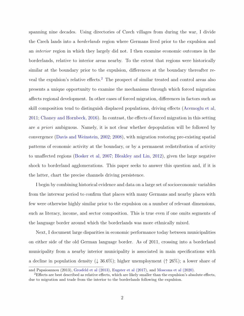
aid of GIS maps of the Protectorate by Jelınek (2011) and 15,070 modern sub-municipal

villages (casti obce), provided by the Czech Statistical Office (CZSO) via its collaboration

with the Czech Land Survey Office (ARCDATA PRAHA, 2017), I create a precise ‘Munich

Agreement line’ (MAL) to measure the German ‘language border’ and sort modern villages

11House prices were about 1 to 3 times annual rent, with 10% down (Wiedemann, 2016; Guzi et al, 2019).

12

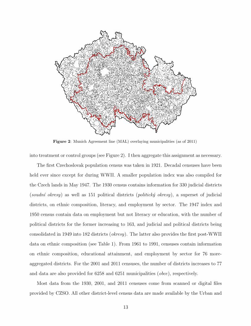
Figure 2: Munich Agreement line (MAL) overlaying municipalities (as of 2011)

into treatment or control groups (see Figure 2). I then aggregate this assignment as necessary.

The first Czechoslovak population census was taken in 1921. Decadal censuses have been

held ever since except for during WWII. A smaller population index was also compiled for

the Czech lands in May 1947. The 1930 census contains information for 330 judicial districts

(soudnı okresy) as well as 151 political districts (politicky okresy), a superset of judicial

districts, on ethnic composition, literacy, and employment by sector. The 1947 index and

1950 census contain data on employment but not literacy or education, with the number of

political districts for the former increasing to 163, and judicial and political districts being

consolidated in 1949 into 182 districts (okresy). The latter also provides the first post-WWII

data on ethnic composition (see Table 1). From 1961 to 1991, censuses contain information

on ethnic composition, educational attainment, and employment by sector for 76 more-

aggregated districts. For the 2001 and 2011 censuses, the number of districts increases to 77

and data are also provided for 6258 and 6251 municipalities (obce), respectively.

Most data from the 1930, 2001, and 2011 censuses come from scanned or digital files

provided by CZSO. All other district-level census data are made available by the Urban and

13

Regional Laboratory (URRlab, 2017) at Charles University in collaboration with the Czech

Ministry of Culture, along with corresponding district shapefiles for each census year. More

disaggregated administrative boundary data come from ARCDATA PRAHA (2017).

Non-census pre-expulsion outcome data come from a variety of sources. I construct 1933

variables using data from state social insurance and taxation reports published in 1938.12

The former provides the number of registered unemployed in each political district, while

the latter lists income and the share of eligible taxpayers by political district. These are

combined with data on the size of the labour force and population from the 1930 census to

estimate 1933 unemployment and income per capita, respectively. Crime data were provided

by URRlab (2017). Historical railway data were provided by HGISe (2020), while roads

data are digitized from a 1930 map produced by the Autoclub of the Czechoslovak Republic

(Autoklub RCS ), shown in Figure A.5 in the Supplemental Material.

For the post-expulsion period, non-census data are digitized from several statistical re-

ports published from the mid-1940s. District-level data for arable land in 1945 and school

enrollment in 1947 are derived from the 1947 and 1948 editions of an annual state statistical

report, respectively. Migration data come from demographic yearbooks made available by

CZSO. Data on abandoned and destroyed structures and settlements come from Zanikle obce

a objekty (2018). Data on the number of jobless by municipality in 2011 were downloaded

from the Czech Ministry of Labour and Social Affairs.

4 The regional economic impact of expulsion

After WWII, around 95% of Germans living in the Czech lands (i.e. the modern day Czech

Republic) were stripped of their citizenship, property rights, and permanently expelled. This

section examines how this impacted former-German places over the long-run. Prior to the

expulsion, those still identifying as German within the Czech lands were concentrated in

one region: the borderlands, or Sudetenland. Although German-speaking had long been

12See the Data Appendix in the Supplemental Material for a full breakdown of all data and their sources.

14

Table 1: Exposure to Expulsion

Region (subsample) % German, 1930 % German, 1950Borderlands (within 25 km of MAL, no overlap) 81.78 4.439

(2.276) (.597)

Interior (within 25 km of MAL, no overlap) 1.601 .495(.396) (.047)

Borderlands (no bandwidth, no overlap) 86.67 6.821(1.646) (1.184)

Interior (no bandwidth, no overlap) 1.646 .464(.418) (.036)

Borderlands (full sample) 80.874 5.36(1.904) (.808)

Interior (full sample) 3.545 .569(.544) (.042)

Notes: Units of observation for 1930 are 330 judicial districts. Units of observation for 1950 are 182 districts. Standard errorsare reported in parentheses. A district is considered to be in the borderlands (interior) if 50% or more of its area lies inside(outside) the lands annexed by Germany in 1938, as determined by the Munich Agreement line (MAL). The full sample includesdistricts that overlap the MAL. A district is classified as ‘no overlap’ if >95% of its area lies on one side of the MAL or theother. A district is classified as ‘within 25 km’ if its centroid lies within 25 km of the MAL. As Prague and Polish Zaolzie arealways excluded from the analysis, I exclude them here as well.

prominent in the corners of the Czech lands, historical developments associated with the rise

of nationalism resulted in this region becoming semi-formal by the 1920s, defined by a spatial

discontinuity in German identification, or ‘language border,’ in official statistics (see Figure

1). This boundary was formalized in 1938, when the Munich Agreement enabled Germany’s

annexation of majority-German areas.

Such dramatic variation in German identification allows me to capture differences in

exposure to the expulsion across local administrative units (e.g. municipalities, districts) and

thus identify the relative effects of the expulsion on the places from which the displacement

occurred. While German identification was grounds for an individual’s expulsion throughout

the Czech lands, regardless of place,13 the proportion of individuals identified as German

and thus expelled in 1945 jumps discontinuously within the Czech lands at the ‘Munich

Agreement line’ (MAL), from 1-2% in interior districts to around 80% in borderland ones,

as shown in Table 1. By 1950, differences had largely disappeared, due to the expulsion.

13Initially, the borderlands likely retained a larger proportion Germans out of need. By the 1950s, however,remaining Germans had either been expelled or dispersed throughout the Czech lands, often out of theborderlands (Gerlach, 2017). Following this and large inflows of interior Czechs into the borderlands, Table1 shows that the share of Germans dropped more in the borderlands from 1930-50, albeit from a larger base.

15

I thus define the treatment variable to be a discrete function of a place’s exposure to

the expulsion by assigning a value of 1 to any municipality or district that was on the

majority-German side of the MAL and a 0 to those in the ‘interior,’ where few Germans

lived. To the extent that other, potentially confounding factors (i.e. historical shocks besides

the expulsion) vary smoothly through the MAL, this will let me identify how places in

which the expulsion occurred were in turn affected, relative to otherwise-similar unaffected

places. This strategy is similar to spatial regression discontinuity (RD), in that it exploits a

discontinuous change in average treatment intensity across space, and is akin to fuzzy RD,

in that variation is discontinuous but not binary.14 However, unlike standard approaches,

treatment assignment for administrative units is also non-binary, given the presence of some

Germans in many predominantly Czechs regions and vice versa. This is similar to Eugster

et al (2017), who use the Swiss language border to capture non-binary cultural variation.

As such, I adopt their language and refer to this approach as a ‘language border contrast’

(LBC). Like spatial RD, this requires certain identifying assumptions be met, which I discuss

in detail in this section. First, I define the standard, municipal-level equation:

ymdb = α + βInBorderlandsm + f(locationm) + X′mΓ + Σb + ∆d + εmdb, (1)

where ymbd is the outcome variable for municipality m in district d along segment b of the

MAL, and InBorderlandsm is the treatment dummy denoting whether municipality m lies

in the borderlands where most Germans lived.15 The remaining terms, discussed below, are

a running variable, f(locationm); a set of geographic characteristics, Xm; a set of border

segment fixed effects, Σb; a set of district fixed effects, ∆d; and an error term, εmdb.

14Later robustness checks sharpen the MAL by dropping mixed areas around it, i.e. areas likely toexperience pre-treatment sorting thus violating standard RD assumptions, and produce similar estimates.

1594 municipalities for which only some parts were annexed are dropped. I define treated as > 95% areaannexed. All specifications and plots exclude those which otherwise overlap the MAL. For 1930-47 analyses,where units are larger such that more area is dropped, results are similar when including units that overlapthe MAL but were nonetheless homogeneously German (i.e. treated in spite of overlap) or non-German –about half of units dropped – as shown in Tables A.5 and A.30.

16

Running variable

The borderlands and interior may exhibit differences in geography, market access, or var-

ious historical experiences, confounding estimates. The purpose of the running variable

f(locationm) is to account for relevant factors besides the treatment that vary across space,

such as these, to the extent that they evolve smoothly at the boundary – an assumption for

which I later argue. If successful, β in equation (1) will estimate effects associated only with

the treatment, holding such factors fixed. In choosing a running variable, many RD designs

begin by limiting the sample to a narrow bandwidth around the border of interest. If this is

feasible given the sample, then a linear running polynomial is often a good approximation,

with minimal noise in estimates (Gelman and Imbens, 2018). As the region of study is quite

small in this setting, all samples are easily limited to 50 km of the MAL, and for most

specifications I adopt a bandwidth of 25 km.16

Another important choice is the variable itself. In order to estimate effects at the bound-

ary, I adopt as my primary running variable a linear polynomial in distance from the MAL,

interacted with the treatment. This focuses the analysis on treated areas that are in closest

proximity to control areas. Further away from the MAL, differences in fundamentals and

other factors such as pre-expulsion labour markets grow, as does the cost of migration for

interior Czechs, rendering sustained regional differences post-expulsion less surprising. I also

include other covariates, as discussed next, to account for spatial heterogeneities that might

influence the effects of being x km from the MAL and, in turn, the estimates of interest.

Another common choice for spatial RD is a two dimensional linear polynomial in longitude

and latitude. Unlike the former approach, this does not account for differences in slope by

treatment status for confounding factors. This may produce biased estimates, as tends to be

the case with non-interacted running variables (Lee and Lemieux, 2010). Furthermore, unlike

with the distance variable, one cannot overcome this by interacting longitude and latitude

with the treatment variable, as then treatment effects would not be estimated at the MAL.

16Increments of 25 km are standard in the prior literature, as optimal bandwidths vary by outcome.

17

This is because while the distance variable is standardized around the boundary in space,

longitude and latitude are not. Nevertheless, I follow Lee and Lemieux (2010) and report

effects using longitude and latitude for completeness, as secondary estimates. Alternative

bandwidth and polynomial approaches are also included in the Supplemental Material.

Covariates and standard errors

The running variable alone may not sufficiently approximate all smooth factors in the pres-

ence of significant spatial heterogeneity. For instance, the gradients of unobservables in

distance from the MAL may vary by region, or they may be too complex for parametric

running polynomials to approximate. I therefore include several additional covariates to

supplement the running variable.

First, main regressions control for a set of exogenous, time-invariant geographic char-

acteristics, including elevation, ruggedness, temperature, precipitation, and rivers (km per

km2).17 Although these appear smooth through the MAL, one concern is that they change

too sizably or frequently in some regions as one moves away from it, in a manner poorly

approximated by a linear trend (see page 44 of the Supplemental Material).18 To the extent

that relevant outcomes are correlated with geography, this could generate false discontinuities

in estimates that disappear once these controls are included. Indeed, estimated differences

for geographic factors themselves go to zero once I condition on the remaining set of geo-

graphic characteristics, as shown in Table 2. That being said, results are generally robust

to excluding such controls.19 Results are also robust to using a restricted sample with only

geographically cohesive (i.e. flat) parts of the Czech lands included, as in Dell (2010).

All main empirical specifications also control for unobservable characteristics using border

segment fixed effects and thus exploit variation within local regions around the MAL. The

17See Dell (2010) and Eugster et al (2017) for similar border analyses utilizing controls.18Also see Table A.2 in the Supplemental Material for unconditional local means and Table A.6 for regres-

sions of geographic variables with running variables but no other geographic controls.19Some coefficients, such as for population density, grow in the expected direction, given the more rugged

nature of the borderlands on average. See Tables A.6, A.13, and A.31 in the Supplemental Material.

18

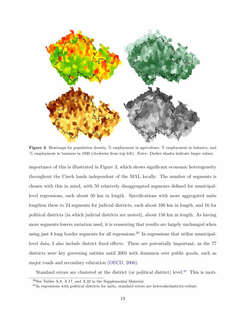
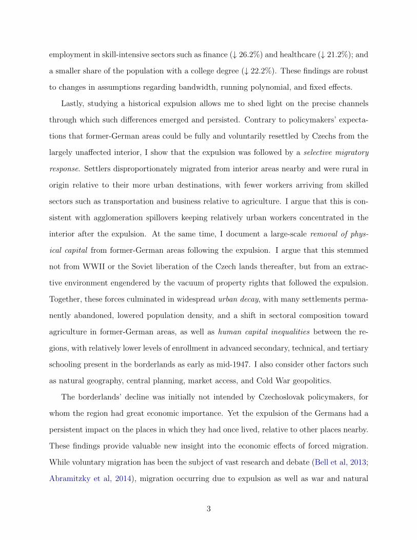
Figure 3: Heatmaps for population density, % employment in agriculture, % employment in industry, and

% employment in business in 1930 (clockwise from top left). Notes: Darker shades indicate larger values.

importance of this is illustrated in Figure 3, which shows significant economic heterogeneity

throughout the Czech lands independent of the MAL locally. The number of segments is

chosen with this in mind, with 50 relatively disaggregated segments defined for municipal-

level regressions, each about 50 km in length. Specifications with more aggregated units

lengthen these to 24 segments for judicial districts, each about 100 km in length, and 16 for

political districts (in which judicial districts are nested), about 150 km in length. As having

more segments lowers variation used, it is reassuring that results are largely unchanged when

using just 8 long border segments for all regressions.20 In regressions that utilize municipal-

level data, I also include district fixed effects. These are potentially important, as the 77

districts were key governing entities until 2003 with dominion over public goods, such as

major roads and secondary education (OECD, 2006).

Standard errors are clustered at the district (or political district) level.21 This is moti-

20See Tables A.8, A.17, and A.32 in the Supplemental Material.21In regressions with political districts for units, standard errors are heteroskedasticity-robust.

19

vated by the role of districts as governing units, such that municipal characteristics are likely

to be correlated within districts. Alternative approaches, including Conley (1999) standard

errors and border segments as clusters, produce similar results (see Table A.18).

Balance testing

In this subsection, I provide evidence that borderland and interior areas were alike at the

MAL in relevant ways prior to the expulsion. Though not essential for the expulsion to

have had real and identifiable effects, it concentrates the analysis on treated and untreated

areas that are highly similar aside from their difference in expulsion experience. This is

advantageous for two reasons. First, it suggests that regions were not differentially exposed

to historical shocks prior to the expulsion that might instead be driving long-run effects.

Second, pre-existing differences have the potential to interact with the treatment in general

equilibrium. For example, if Germans and Czechs worked in very different sectors, or if

places with many Germans had very different natural factors, then the set of Czechs who

could feasibly resettle those areas in the short-run would be more limited, diminishing the

prospect of long-run convergence at the boundary.

Section 2 detailed how, following centuries of admixture and common rule, Germans and

Czechs exhibited few social or economic differences in the early 1900s, with the develop-

ments that gave rise to the MAL and eventual expulsion rooted in national rather than

economic considerations (Zahra, 2008). To test this, I examine whether the MAL and the

ethnolinguistic differences for which it was drawn were associated prior to the expulsion with

differences in factors such as education, labour market factors, and institutions at the MAL,

where other relevant factors such as natural geography are fixed.

I begin by reaffirming that the MAL identifies German identification and thus exposure

to the expulsion. Table 2 shows that traversing the MAL was associated with an increase of

about 68 percentage points (pp) in the German population in 1930. In contrast, it coincides

with statistically significant differences for no other factor in primary specifications.

20

Table 2: Pre-expulsion Economic Differences Between Regions

%GermanLiteracy

rateln Pop.density

Labourforce part.

Unemploy-ment rate

Incomepc

(1a) (1b) (1c) (1d) (1e) (1f)In borderlands 67.968 -.222 -.318 -.400 -3.936 -1.866(linear in distance) (6.042)∗∗∗ (.217) (.208) (1.196) (2.535) (1.832)

R2 .933 .533 .475 .623 .69 .409In borderlands 73.575 .264 -.108 .631 1.781 -.392(linear in x and y) (3.853)∗∗∗ (.152)∗ (.116) (.769) (2.449) (1.490)

R2 .933 .515 .482 .633 .645 .387Mean dep. var. 1.601 98.385 4.764 45.386 9.791 9.428in interior (3.760) (.669) (.733) (4.622) (10.028) (4.661)Observations 165 165 165 165 104 104Clusters 98 98 98 98 – –Border segments 24 24 24 24 16 16Bandwidth 25 km 25 km 25 km 25 km 50 km 50 kmYear 1930 1930 1930 1930 1933 1933

%TaxpayersConvictspc,

1923-27%Roma %Jewish

Roads (km)per sq. km

Rail (km)per sq. km

(2a) (2b) (2c) (2d) (2e) (2f)In borderlands .006 -.454 -.002 -.113 .014 .005(linear in distance) (.604) (.683) (.002) (.140) (.016) (.009)

R2 .562 .361 .1 .324 .311 .393In borderlands .391 .230 -.001 .064 .004 .010(linear in x and y) (.484) (.404) (.001) (.068) (.011) (.008)

R2 .541 .337 .112 .328 .302 .406Mean dep. var. 5.680 7.273 .001 .182 .216 .096in interior (1.981) (2.058) (.006) (.477) (.074) (.065)Observations 105 164 165 165 271 271Clusters – 98 98 98 107 107Border segments 16 24 24 24 24 24Bandwidth 50 km 25 km 25 km 25 km 25 km 25 kmYear 1933 1923-27 1930 1930 1930 1930

Elevation Ruggedness Precipitation TemperatureRivers (km)per sq. km

% Arableland, 1945

(3a) (3b) (3c) (3d) (3e) (3f)In borderlands .509 .064 .108 .001 -.061 .279(linear in distance) (2.630) (.245) (.233) (.016) (.048) (4.542)

R2 .994 .58 .978 .993 .336 .707In borderlands .112 .059 .452 .002 -.007 -1.340(linear in x and y) (1.743) (.243) (.236)∗ (.009) (.048) (3.664)

R2 .995 .585 .982 .995 .333 .716Mean dep. var. 398.881 6.093 53.104 7.650 1.141 51.181in interior (133.667) (2.840) (6.839) (.709) (.527) (12.152)Observations 4049 4049 4049 4049 4049 115Clusters 71 71 71 71 71 –Border segments 50 50 50 50 50 16Bandwidth 25 km 25 km 25 km 25 km 25 km 50 km

Robust standard errors are clustered by political district, with ***, **, and * denoting significance at the 1%, 5%, and 10%levels, respectively. Notes: All regressions exclude Prague and Polish Zaolzie, include border segment fixed effects as wellas exogenous controls for elevation, ruggedness, precipitation, temperature, and river density (km per km2), except whenused as an outcome variable, and utilize a local linear running variable of either distance from the Munich Agreement lineinteracted with the treatment or longitude and latitude. Units of observation are judicial districts, except unemployment,income, and taxpayers, which use political districts, a superset of judicial districts; time-invariant geographic outcomes, whichuse municipalities; and road and railway densities, which use judicial districts ‘parts,’ derived in ArcGIS according to the ‘splitsample analysis’ described in the Supplemental Material. Average 1933 income per capita is in units of 100 Czechoslovakkoruna. Average convicts per capita indicates the number of convicted offenders in Czech criminal districts between 1923 and1927 as a proportion of the total population in 1930. All shares are out of 100.

21

Table 3: Pre-expulsion Sectoral Differences Between Regions

Agriculturalsector

Mining andextraction

MetalsMachineryand auto

Glass Textiles

(1a) (1b) (1c) (1d) (1e) (1f)In borderlands 2.915 -1.150 .455 -.421 1.065 -3.311(linear in distance) (3.649) (1.698) (1.458) (.561) (1.681) (2.534)

R2 .526 .376 .313 .298 .338 .634In borderlands -1.264 -.982 -.414 -.697 .230 .758(linear in x and y) (2.577) (.970) (.911) (.324)∗∗ (.479) (1.552)

R2 .535 .395 .339 .311 .35 .64Mean dep. var. 30.713 3.510 4.818 2.631 .674 5.586in interior (12.800) (4.568) (3.793) (2.187) (1.891) (9.646)

Otherindustry

Con-struction

Transportsector

Finance andinsurance

TradeOtherservice

(2a) (2b) (2c) (2d) (2e) (2f)In borderlands .102 .500 -.457 -.110 -.534 -.355(linear in distance) (1.429) (.719) (.665) (.094) (.796) (.927)

R2 .315 .332 .318 .258 .377 .209In borderlands -.702 .339 -.114 -.015 .498 .722(linear in x and y) (1.062) (.568) (.420) (.056) (.416) (.643)

R2 .275 .336 .321 .245 .356 .175Mean dep. var. 14.985 6.744 3.560 .428 5.151 6.394in interior (5.403) (1.862) (2.153) (.350) (1.722) (3.662)Observations 165 165 165 165 165 165Clusters 98 98 98 98 98 98Border segments 24 24 24 24 24 24Bandwidth 25 km 25 km 25 km 25 km 25 km 25 kmYear 1930 1930 1930 1930 1930 1930

Robust standard errors are clustered by political district, with ***, **, and * denoting significance at the 1%, 5%, and 10%levels, respectively. Notes: All regressions exclude Prague and Polish Zaolzie, include border segment fixed effects as well asexogenous controls for elevation, ruggedness, precipitation, temperature, and river density (km per km2), and utilize a locallinear running variable of either distance from the Munich Agreement line interacted with the treatment or longitude andlatitude. Units of observation are judicial districts. All outcomes represent the share (out of 100) of the labour force in a sector.

22

First, Czech and German speakers in the Czech lands appear to be ‘well-matched’ in

terms of education, consistent with the historical evidence laid out in Section 2, with literacy

rates in 1930 of around 98% on both sides of the MAL (Zahra, 2008, 18). Despite some

regional differences in educational content, this reflects the high educational standards of

the Czechoslovak system with respect to all individuals.

Pre-expulsion labour markets also exhibit smoothness through the MAL, a fact that

speaks favorably to the potential resettlement of the borderlands by nearby interior Czechs.

Consistent with the historical literature, sectors do not appear to vary significantly at the

MAL in Table 3, including for German-dominated industries overall such as glassworks

and textile manufacturing. Unemployment, which affected German-speaking areas closer to

Germany more severely during the Depression, is likewise smooth through the MAL, where

the industrial composition of Czech and German speakers was more similar, as are other

labour market outcomes such as income. One exception is the machine and auto industry,

which exhibits a decrease in the secondary specification, although no other running variable

assumptions generate such significance.22 These alternative specifications as well as plots of

all outcome variables are available in the Supplemental Material.

Lastly, though more difficult to test, the results here are consistent with the historical

literature in downplaying local differences in institutions. The relative egalitarianism of the

Czech lands across ethnic groups is apparent in the regions’ similar taxation and criminal

conviction levels, as shown above. Another indicator of such egalitarianism comes from

examining market access, as measured by transport availability. As it is plausible that major

road and rail connections might have been fewer in the borderlands, I examine balance tests

for both major roads and railways per square km. A lack of smoothness would likely have had

implications for long-run effects, as transport integration would have been key to minimizing

differences between the regions after the expulsion. Table 2 shows both to be highly smooth

22Some estimates, namely for population density, are likely to be correlated with geography and indeedgain in significance when these controls are dropped, showcasing their importance. For these estimates, seeTable A.6 in the Supplemental Material.

23

through the MAL as of 1930. Estimates are similar for rails using data from 1940, but, as

that data are less reliable, I do not feature them here.23 Figure A.4 in the Supplemental

Material maps these connections for both years, while Figure A.5 shows major roads in 1930.

Overall, these results corroborate the notion that Germans and Czechs in the Czech lands

were highly similar after centuries of coexistence, as argued by historians – as well as by the

Nazis during WWII (Bryant, 2007).

Other concerns: WWII, pre-treatment sorting, and borderland Czechs

The same nationalism that motivated the expulsion also inspired the annexation of the

borderlands and occupation of Czechoslovakia by Nazi Germany a few years prior. Yet

one concern is that such events and others during WWII might have differentially affected

borderland areas near the MAL. Indeed, a major limitation in studying this era is the lack

of data from during the war. I address these concerns here.

Following annexation and occupation, the Czech government was exiled and preferential

treatment of the Czech regions by the Nazis during the war would have favored the border-

lands, biasing estimates toward zero. That being said, both the borderlands and interior

experienced little physical destruction during the war, with Czech civilian casualties from

such of about 10,000 (Erlikhman, 2004).24 There were also few acts of resistance by Czechs.

Czechs made up a large and important industrial workforce, and Nazi officials saw much of

the Czech masses as ‘Germanizable’ due to their cultural and genetic proximity. Thus, life

in the Czech interior continued largely as normal, avoiding much of the violence experienced

by Yugoslavia and Poland (Agnew, 2004; Bryant, 2007; Glassheim, 2016). Economic life in

the borderlands also changed little, at the displeasure of some borderland Germans, who

had sought greater integration into the German economy and society. In all, ‘Czechoslovakia

emerged from the war with much of its industrial base intact’ (Gerlach, 2017, 208).

23This is according to the creators of the dataset. For completeness, I do include the 1940 estimates inTable A.35 in the Supplemental Material; they are similar.

24Sudeten German civilian casualty counts are uncertain, but few bombs struck the borderlands. SeeFigure A.3 for a map of confirmed Allied WWII bombings. See Table A.3 for more on casualty estimates.

24

Differences in military deaths are more difficult to discern. Historical accounts suggest the

borderlands suffered more in terms of war casualties than the interior, due to conscription of

Sudeten Germans. A more recent estimate by Overmans (2004) places the number of German

war dead from all annexed territories, including annexed Poland, at 206,000. However, counts

are complicated by the fact that many deaths occurred during the violent liberation of

Czechoslovakia in May 1945, which also marked the first expulsions. Separately, many Jews

and Roma were expelled from or murdered in the Czech lands during this time. However,

these groups were distributed uniformly through the MAL, as shown in Table 2.25 Thus,

pre-1945 casualty rate differences between the regions were likely small on net.

Another concern is related to the non-binary nature of treatment assignment. Unlike

the interior, which by 1930 was strikingly homogeneous (at least officially), some parts of

the borderlands were quite mixed, especially near the MAL. Some of this was rooted in

pre-treatment sorting by Czechs. According to historians, such migrations occurred several

times – first by interior Czechs immigrating to some borderland cities after 1918, then by

300,000 of the 730,000 borderland Czechs into the interior during the war, and finally by

nearly all of those Czechs back into the borderlands after the war (Cornwall, 1994; Agnew,

2004; Glassheim, 2016). This could bias effects if it was driven by relevant factors.

Pre-treatment sorting, and the presence of borderland Czechs more broadly, may also

make balance tests less useful for evaluating the historical similarity of more and less treated

areas, as it would mean that cross-region differences are not necessarily informative of cross-

ethnic differences. For example, if Czechs near the MAL were in fact less skilled than

Germans, borderland Czechs could bias literacy estimates from positive to zero.

How can one determine the importance of pre-treatment sorting and borderland Czechs

in driving pre-expulsion similarities as well as effects? Since I cannot compare Czechs and

Germans directly, I rely on heterogeneity in the ethnic composition of the borderlands prior to

the expulsion to better compare Czechs and Germans at the MAL. In particular, I reexamine

25Estimates are similar if I instead use a measure of Jewish religious identification; see Figure A.6 in theSupplemental Material for this data plotted.

25

Table 4: Long-run Differences in Economic Activity, 2011

ln Populationdensity

ln Labour forcedensity

Unemploymentrate

(1a) (1b) (1c)In borderlands -.312 -.317 2.729(linear in distance) (.095)∗∗∗ (.097)∗∗∗ (.546)∗∗∗

R2 .398 .399 .404In borderlands -.251 -.253 3.623(linear in x and y) (.084)∗∗∗ (.086)∗∗∗ (.520)∗∗∗

R2 .4 .4 .398Mean dep. var. 4.034 3.294 10.492in interior (.885) (.911) (4.809)Observations 4049 4049 4049Clusters 71 71 71Border segments 50 50 50Bandwidth 25 km 25 km 25 kmYear 2011 2011 2011

Robust standard errors are clustered by district, with ***, **, and * denoting significance at the 1%, 5%, and 10% levels,respectively. Notes: All regressions exclude Prague and Polish Zaolzie, include border segment and district fixed effects aswell as exogenous controls for elevation, ruggedness, precipitation, temperature, and river density (km per km2), and utilize alocal linear running variable of either distance from the Munich Agreement line interacted with the treatment or longitude andlatitude. Units of observation are municipalities.

the balance tests above using a sample of ‘discrete’ stretches of the MAL, in which I compare

only homogeneous parts of the interior with nearby, homogeneous parts of the borderlands

with few borderland Czechs (and thus little pre-treatment sorting).

In Table A.7 in the Supplemental Material, I show that while this increases the size of

the ethnic discontinuity to 86 pp, estimates regarding relative literacy, population density,

and sector composition change little. One exception, eligible taxpayers, now shows a sta-

tistically significant increase from crossing MAL in both specifications tested, of 1.6 eligible

taxpayers per 100 persons. Yet Czechs and Germans overall still appear quite similar as

compared across homogeneous districts. Moreover, long-run effects do not appear to be bi-

ased by pre-treatment sorting or the presence of borderland Czechs, with full and discrete

samples yielding similar results.26 This reaffirms the notion that Czechs, Germans, and their

respective places were similar in relevant ways prior to the expulsion, at least at the MAL.27

26See Table A.16 in the Supplemental Material. I also estimate pre-trends at the MAL using both fulland discrete samples, as shown in Table A.11. Development trajectories of Germans and Czechs between1921-30 are overall similar, although I do estimate relative increases in literacy among Germans.

27And in addition to the kinds of pre-treatment sorting discussed above, this exercise reaffirms that the

26

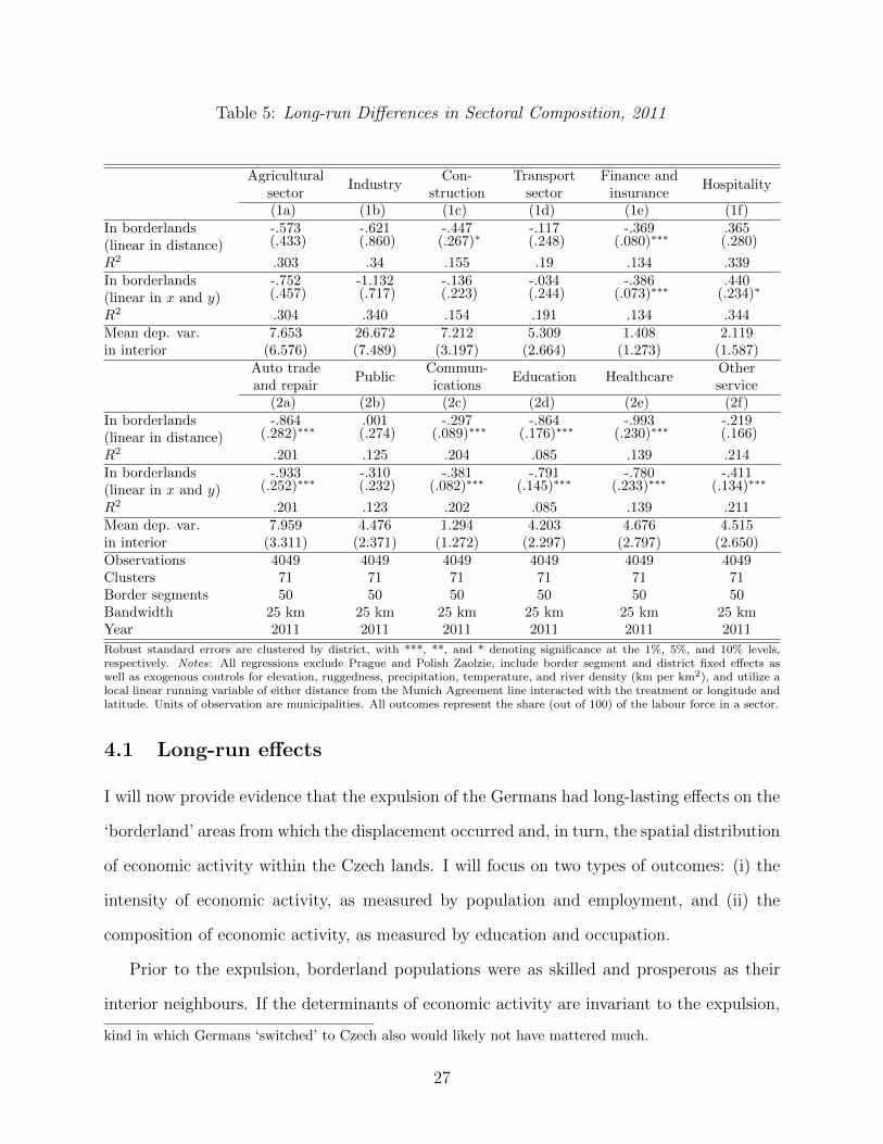
Table 5: Long-run Differences in Sectoral Composition, 2011

Agriculturalsector

IndustryCon-

structionTransport

sectorFinance and

insuranceHospitality

(1a) (1b) (1c) (1d) (1e) (1f)In borderlands -.573 -.621 -.447 -.117 -.369 .365(linear in distance) (.433) (.860) (.267)∗ (.248) (.080)∗∗∗ (.280)

R2 .303 .34 .155 .19 .134 .339In borderlands -.752 -1.132 -.136 -.034 -.386 .440(linear in x and y) (.457) (.717) (.223) (.244) (.073)∗∗∗ (.234)∗

R2 .304 .340 .154 .191 .134 .344Mean dep. var. 7.653 26.672 7.212 5.309 1.408 2.119in interior (6.576) (7.489) (3.197) (2.664) (1.273) (1.587)

Auto tradeand repair

PublicCommun-ications

Education HealthcareOtherservice

(2a) (2b) (2c) (2d) (2e) (2f)In borderlands -.864 .001 -.297 -.864 -.993 -.219(linear in distance) (.282)∗∗∗ (.274) (.089)∗∗∗ (.176)∗∗∗ (.230)∗∗∗ (.166)

R2 .201 .125 .204 .085 .139 .214In borderlands -.933 -.310 -.381 -.791 -.780 -.411(linear in x and y) (.252)∗∗∗ (.232) (.082)∗∗∗ (.145)∗∗∗ (.233)∗∗∗ (.134)∗∗∗

R2 .201 .123 .202 .085 .139 .211Mean dep. var. 7.959 4.476 1.294 4.203 4.676 4.515in interior (3.311) (2.371) (1.272) (2.297) (2.797) (2.650)Observations 4049 4049 4049 4049 4049 4049Clusters 71 71 71 71 71 71Border segments 50 50 50 50 50 50Bandwidth 25 km 25 km 25 km 25 km 25 km 25 kmYear 2011 2011 2011 2011 2011 2011

Robust standard errors are clustered by district, with ***, **, and * denoting significance at the 1%, 5%, and 10% levels,respectively. Notes: All regressions exclude Prague and Polish Zaolzie, include border segment and district fixed effects aswell as exogenous controls for elevation, ruggedness, precipitation, temperature, and river density (km per km2), and utilize alocal linear running variable of either distance from the Munich Agreement line interacted with the treatment or longitude andlatitude. Units of observation are municipalities. All outcomes represent the share (out of 100) of the labour force in a sector.

4.1 Long-run effects

I will now provide evidence that the expulsion of the Germans had long-lasting effects on the

‘borderland’ areas from which the displacement occurred and, in turn, the spatial distribution

of economic activity within the Czech lands. I will focus on two types of outcomes: (i) the

intensity of economic activity, as measured by population and employment, and (ii) the

composition of economic activity, as measured by education and occupation.

Prior to the expulsion, borderland populations were as skilled and prosperous as their

interior neighbours. If the determinants of economic activity are invariant to the expulsion,

kind in which Germans ‘switched’ to Czech also would likely not have mattered much.

27

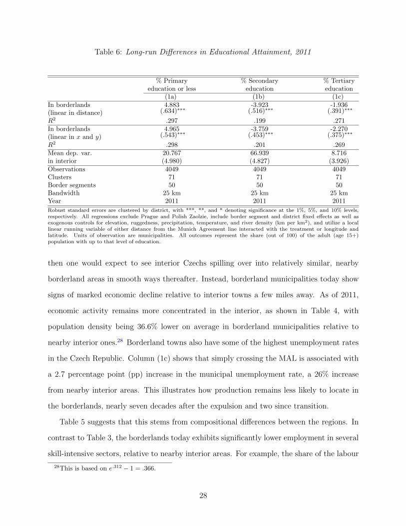
Table 6: Long-run Differences in Educational Attainment, 2011

% Primaryeducation or less

% Secondaryeducation

% Tertiaryeducation

(1a) (1b) (1c)In borderlands 4.883 -3.923 -1.936(linear in distance) (.634)∗∗∗ (.516)∗∗∗ (.391)∗∗∗

R2 .297 .199 .271In borderlands 4.965 -3.759 -2.270(linear in x and y) (.543)∗∗∗ (.453)∗∗∗ (.375)∗∗∗

R2 .298 .201 .269Mean dep. var. 20.767 66.939 8.716in interior (4.980) (4.827) (3.926)Observations 4049 4049 4049Clusters 71 71 71Border segments 50 50 50Bandwidth 25 km 25 km 25 kmYear 2011 2011 2011

Robust standard errors are clustered by district, with ***, **, and * denoting significance at the 1%, 5%, and 10% levels,respectively. All regressions exclude Prague and Polish Zaolzie, include border segment and district fixed effects as well asexogenous controls for elevation, ruggedness, precipitation, temperature, and river density (km per km2), and utilize a locallinear running variable of either distance from the Munich Agreement line interacted with the treatment or longitude andlatitude. Units of observation are municipalities. All outcomes represent the share (out of 100) of the adult (age 15+)population with up to that level of education.

then one would expect to see interior Czechs spilling over into relatively similar, nearby

borderland areas in smooth ways thereafter. Instead, borderland municipalities today show

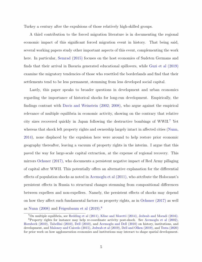
signs of marked economic decline relative to interior towns a few miles away. As of 2011,

economic activity remains more concentrated in the interior, as shown in Table 4, with

population density being 36.6% lower on average in borderland municipalities relative to

nearby interior ones.28 Borderland towns also have some of the highest unemployment rates

in the Czech Republic. Column (1c) shows that simply crossing the MAL is associated with

a 2.7 percentage point (pp) increase in the municipal unemployment rate, a 26% increase

from nearby interior areas. This illustrates how production remains less likely to locate in

the borderlands, nearly seven decades after the expulsion and two since transition.

Table 5 suggests that this stems from compositional differences between the regions. In

contrast to Table 3, the borderlands today exhibits significantly lower employment in several

skill-intensive sectors, relative to nearby interior areas. For example, the share of the labour

28This is based on e.312 − 1 = .366.

28

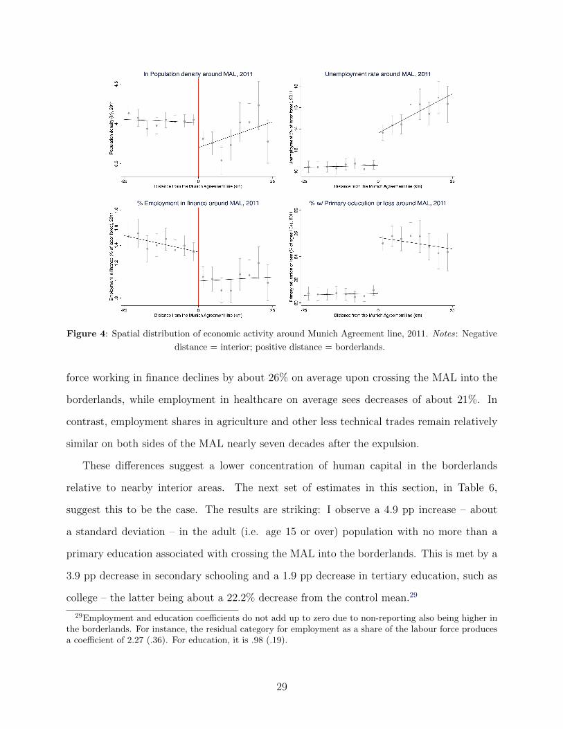
Figure 4: Spatial distribution of economic activity around Munich Agreement line, 2011. Notes: Negative

distance = interior; positive distance = borderlands.

force working in finance declines by about 26% on average upon crossing the MAL into the

borderlands, while employment in healthcare on average sees decreases of about 21%. In

contrast, employment shares in agriculture and other less technical trades remain relatively

similar on both sides of the MAL nearly seven decades after the expulsion.

These differences suggest a lower concentration of human capital in the borderlands

relative to nearby interior areas. The next set of estimates in this section, in Table 6,

suggest this to be the case. The results are striking: I observe a 4.9 pp increase – about

a standard deviation – in the adult (i.e. age 15 or over) population with no more than a

primary education associated with crossing the MAL into the borderlands. This is met by a

3.9 pp decrease in secondary schooling and a 1.9 pp decrease in tertiary education, such as

college – the latter being about a 22.2% decrease from the control mean.29

29Employment and education coefficients do not add up to zero due to non-reporting also being higher inthe borderlands. For instance, the residual category for employment as a share of the labour force producesa coefficient of 2.27 (.36). For education, it is .98 (.19).

29

Results do not meaningfully change if one considers only geographically cohesive or previ-

ously homogeneous parts of the Czech lands, reaffirming that geography and the non-binary

treatment assignment are not driving effects. Results are also robust to using longer or

no border segments, dropping district fixed effects, dropping controls, modifying bandwidth

and running variable assumptions, clustering by border segment, and using Conley standard

errors with various bandwidths (see Tables A.12-18 in the Supplemental Material).

5 Channels

The previous section documented relatively depressed levels of economic activity in the Czech

borderlands, nearly 70 years after its German population was expelled. This section inves-

tigates the channels through which regional disparities originated. Since no unevenness was

present prior to the expulsion, I begin by examining the economic activity of those who vol-

untarily resettled the borderlands from interior areas immediately following the expulsion,

relative to those who did not. Indeed, the expulsion’s impact on the borderlands’ relative

development depended on it being resettled in a quick and convergent manner. To compare

these populations, I use data from after the expulsion and the borderlands’ initial resettle-

ment had concluded in mid-1947.30 This will also allow me to establish whether or not key

structural changes had occurred prior to the advent of central planning in 1948. I then use

longer-run data to study the subsequent persistence of effects.

In this section, I show that the expulsion was instead followed by a (i) selective initial

resettlement. Settlers disproportionately migrated from interior areas nearby and were rural

in origin relative to their more urban destinations, with fewer workers arriving from skilled

sectors such as business relative to agriculture. I argue that this is consistent with agglom-

eration economies keeping relatively urban workers concentrated in the interior after the

expulsion. Simultaneously, I document a large-scale (ii) loss of physical capital in former-

30The historical literature indicates that the 5% or so remaining were largely skilled workers initially keptout of need, potentially downward biasing 1947 estimates slightly.

30

German areas following the expulsion. I argue that this stemmed not from WWII or the

Soviet liberation of the Czech lands thereafter, but from an extractive environment engen-

dered by the vacuum of property rights that followed the expulsion. Together, these factors

culminated in (iii) urban decay, with many settlements permanently abandoned, lowered

population density, and a shift in sectoral composition toward agriculture in former-German

areas, as well as (iv) human capital inequalities between the regions thereafter. While this

analysis will focus on the events of the immediate post-expulsion period, during which the

Czechoslovak economy remained generally unplanned, I will also discuss how these patterns

evolved during the communist period and following transition to a market economy in 1989.

5.1 Selective resettlement

The effects of the expulsion – on former-German areas but also in general equilibrium –

depended on the German population first being replaced by interior settlers, in both count

and composition. The stated goal of resettlement was that it be geographically convergent :

since the expulsion ‘would reduce the Czechoslovakia population by 25%, the borderlands

would only be resettled up to 75% of [its] original population,’ preserving prewar relative

densities while creating one homogeneous nation (Radvanovsky, 2001, 203). This was to be

done quickly and concurrently with the expulsion, with the goal of maintaining the region’s

output (Glassheim, 2016). It was also to be carried out on a voluntary basis. Policymakers

used German property, confiscated without payment and reallocated at low rates, in addition

to various incentives, as discussed in Section 2. Besides such interventions, worker and firm-

level decisions remained unplanned until the communist coup of 1948 (Bernasek, 1970).

Under such circumstances, one possible migratory response to the expulsion would be a

convergent one, at least at the MAL, with interior Czechs migrating to replace Germans with

relatively similar labour endowments. Indeed, one might expect the expulsion to have made

the borderlands an attractive place in which to settle and invest, given its proximity, factor

similarities, and the large amounts of former-German land and property available there.

31

Figure 5: Sources of immigration to Northern Bohemia (dotted region), 1945-7. Notes: Migrant data

sourced from figure in ‘Osıdlenı pohranicı v letech 1945-1952’ (1953), reprinted in von Arburg (2001).

As it turns out, the expulsion was met with a large-scale migratory response, beginning

in mid-1945 through the first half of 1947. However, this initial resettlement was selective

in nature, in both (i) location and (ii) occupation. To see this, one can compare population

losses endured by the interior (i.e. to the voluntary resettling of the borderlands) with those

of borderland areas (i.e. from the expulsion net of resettlement) along these dimensions.

Locational selection among settlers

Understanding where Czech migrants settled within the borderlands after the expulsion, as

well as from where they originated in the interior, is of primary importance for understanding

how the expulsion affected not just former-German areas, but the economic geography of

the Czech lands overall. To do this, I construct an outcome variable to measure population

losses in each judicial district d between the 1930 census and mid-1947 index:

PopChanged =Popd,1947 − Popd,1930

Popd,1930

.

32

To the extent that nearby borderland and interior districts had similar characteristics and

trends prior to the expulsion, including few shocks of permanence or scale during WWII,

the convergent migratory response envisioned by policymakers would have required that

such losses be similar for each region by the time expulsion and the borderlands’ initial

resettlement had wound down in mid-1947, relative to pre-expulsion levels.

In addition to the treatment dummy indicating a district’s region, I exploit two further

measures of location to predict population dynamics: (i) distance from the MAL and (ii)

being within 25 km of a city with 50,000+ residents in 1930, both of which I interact with

the treatment, and where applicable each other, to allow for heterogeneous effects.

The baseline results in Table 7 show a lack of convergence at the MAL in mid-1947,

contrary to policymaker expectations: while both regions lost in population on net, border-

land districts had still lost about 13.5 pp more on average post-resettlement than nearby

interior districts.31 As one moves away from the MAL, interior losses shrink, suggesting

resettlement to be driven by interior settlers coming from near the MAL. This is consistent

with the historical evidence. For instance, Figure 5 illustrates the largely nearby interior

sources of settlers to the Northern Bohemian borderlands, as detailed in a 1953 official state

report. I also consider specifications with a 50 km bandwidth to evaluate trends beyond the

25 km bandwidth. These, in columns (2), show population losses to also be growing more in

the borderlands further from the MAL. Altogether, this suggests that location-specific hu-

man capital may have been important in driving resettlement, with Czechs migrating from

interior areas with similar factor endowments.

Convergence was also more likely conditional on borderland districts being more urban

historically. In particular, the interaction effect for being near a major 1930 urban area

is positive and significant, while the corresponding baseline term tends to be smaller and

insignificant. This also suggests that migration from the interior to the borderlands after

the expulsion was not driven by urban interior residents moving to urban borderland areas,

31While it is possible that more settlers coming from abroad or Slovakia were of those sectors, these madeup a tiny fraction of settlers and would only have made the borderlands’ relative declines appear smaller.

33

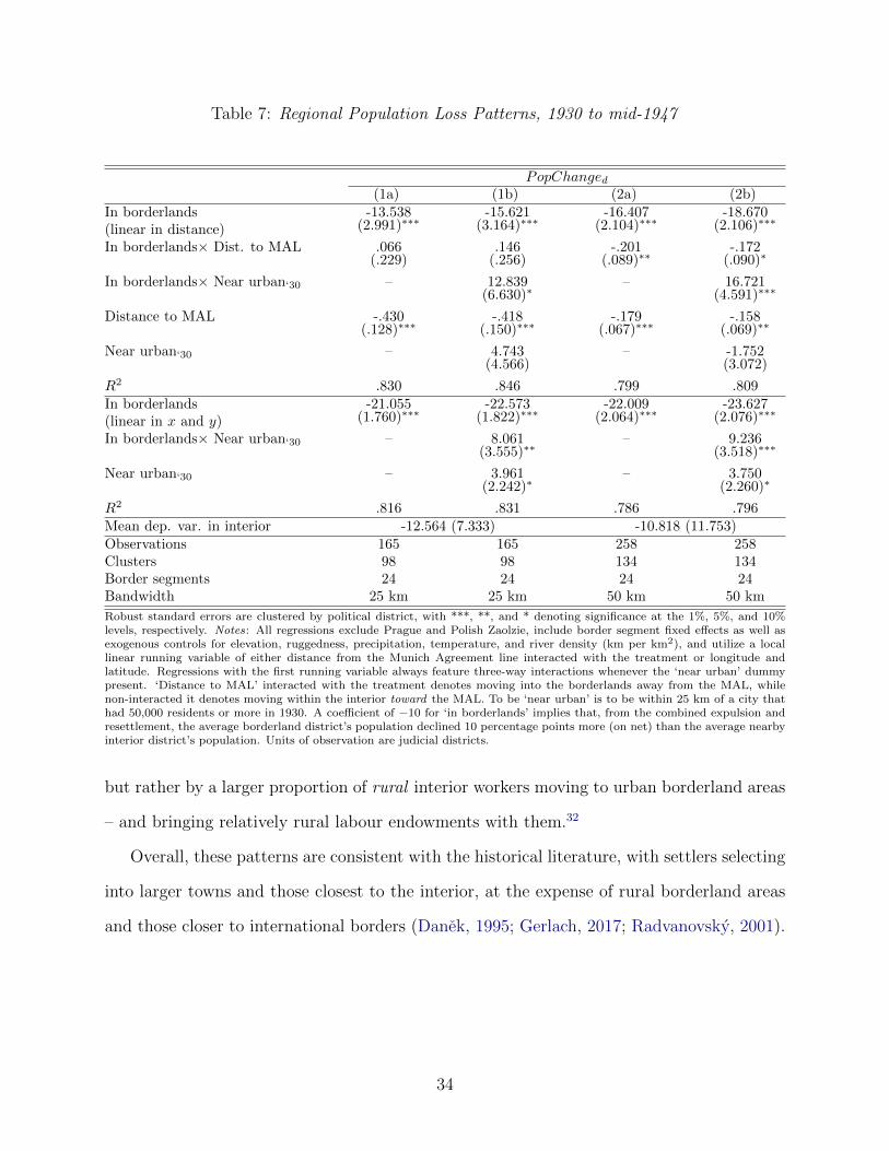
Table 7: Regional Population Loss Patterns, 1930 to mid-1947

PopChanged(1a) (1b) (2a) (2b)

In borderlands -13.538 -15.621 -16.407 -18.670(linear in distance) (2.991)∗∗∗ (3.164)∗∗∗ (2.104)∗∗∗ (2.106)∗∗∗

In borderlands× Dist. to MAL .066 .146 -.201 -.172(.229) (.256) (.089)∗∗ (.090)∗

In borderlands× Near urban‘30 – 12.839 – 16.721(6.630)∗ (4.591)∗∗∗

Distance to MAL -.430 -.418 -.179 -.158(.128)∗∗∗ (.150)∗∗∗ (.067)∗∗∗ (.069)∗∗

Near urban‘30 – 4.743 – -1.752(4.566) (3.072)

R2 .830 .846 .799 .809In borderlands -21.055 -22.573 -22.009 -23.627(linear in x and y) (1.760)∗∗∗ (1.822)∗∗∗ (2.064)∗∗∗ (2.076)∗∗∗

In borderlands× Near urban‘30 – 8.061 – 9.236(3.555)∗∗ (3.518)∗∗∗

Near urban‘30 – 3.961 – 3.750(2.242)∗ (2.260)∗

R2 .816 .831 .786 .796Mean dep. var. in interior -12.564 (7.333) -10.818 (11.753)Observations 165 165 258 258Clusters 98 98 134 134Border segments 24 24 24 24Bandwidth 25 km 25 km 50 km 50 km

Robust standard errors are clustered by political district, with ***, **, and * denoting significance at the 1%, 5%, and 10%levels, respectively. Notes: All regressions exclude Prague and Polish Zaolzie, include border segment fixed effects as well asexogenous controls for elevation, ruggedness, precipitation, temperature, and river density (km per km2), and utilize a locallinear running variable of either distance from the Munich Agreement line interacted with the treatment or longitude andlatitude. Regressions with the first running variable always feature three-way interactions whenever the ‘near urban’ dummypresent. ‘Distance to MAL’ interacted with the treatment denotes moving into the borderlands away from the MAL, whilenon-interacted it denotes moving within the interior toward the MAL. To be ‘near urban’ is to be within 25 km of a city thathad 50,000 residents or more in 1930. A coefficient of −10 for ‘in borderlands’ implies that, from the combined expulsion andresettlement, the average borderland district’s population declined 10 percentage points more (on net) than the average nearbyinterior district’s population. Units of observation are judicial districts.

but rather by a larger proportion of rural interior workers moving to urban borderland areas

– and bringing relatively rural labour endowments with them.32

Overall, these patterns are consistent with the historical literature, with settlers selecting

into larger towns and those closest to the interior, at the expense of rural borderland areas

and those closer to international borders (Danek, 1995; Gerlach, 2017; Radvanovsky, 2001).

34

Occupational selection among settlers

Given the above findings, it is unsurprising that migratory sorting also occurred on sectoral

lines. This can be seen in Figure 6, which charts PopChanged overall and by sector, both

at and away from the MAL. These show differences in worker losses around the MAL were

relatively small for agriculture and large for other, more ‘urban’ sectors such as business.

This is consistent with the historical narrative that settlers were disproportionately unskilled

farmers, with settlement initiatives struggling to attract skilled workers while interior areas

suffered shortages in agricultural labour (Radvanovsky, 2001; Gerlach, 2017). Differences in

net losses between regions again shrink as one approaches the MAL. LBC estimates can be

found in Table A.20 in the Supplemental Material.33

The sources of the patterns in this section are undoubtedly multifarious. In the pres-

ence of agglomeration economies, for instance, such a large population shock would have

generated a massive spatial coordination problem for the remaining population, potentially

decreasing the expected relative return to migrating to borderland towns for workers in ur-

ban sectors in the short-run – albeit less so where locational fundamentals were similar and

where settlements were more populous historically (Allen and Donaldson, 2018). Moreover,

with a convergent initial resettlement inhibited, such ‘core-periphery’ regional patterns could

become locked in (Krugman, 1991, Puga, 1999). Indeed, data from the 1930s suggest the

presence of strong agglomeration economies throughout the pre-expulsion Czech lands, with

population density strongly positively correlated with income and employment in industry,

transport, and business, and negatively with employment in agriculture, consistent with the

selection above.34 That being said, this need not be the entire story, as I will argue now.

32I use a 25,000 population threshold in Table A.19. Results are similar, though urban effects are weaker.33Other compositional factors, such as sex, were not selected upon, although historians have noted that

settlers tended to be younger (Gerlach, 2017). I find no evidence in the 1947 data of selection on sex, thoughI do estimate a 7.8 (1.1) pp increase from crossing the MAL in the share of the population that is under theage of 15 in mid-1947, something not present in the 1930 data.

34Table A.21 shows these correlations, with magnitudes independent of region. Figure A.11 also shows asignificant degree of localization along sector lines in 1930, with industry featuring prominently in NorthernMoravia and business in Northern Bohemia, which would have been severely disrupted by the expulsion.

35

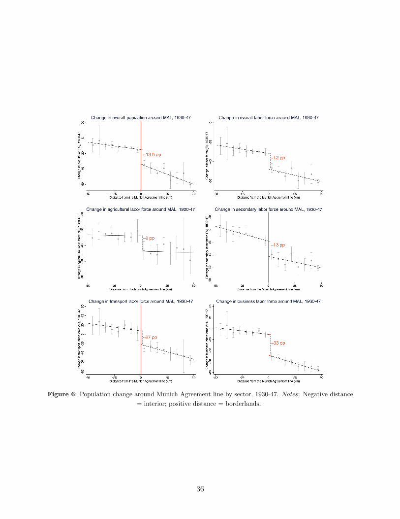
Figure 6: Population change around Munich Agreement line by sector, 1930-47. Notes: Negative distance

= interior; positive distance = borderlands.

36

Figure 7: Abandoned or destroyed industrial structures (Zanikle obce a objekty, 2018)

5.2 Physical capital extraction

Unlike voluntary outmigration events, forced migrations – including both expulsions and

those from natural disaster – often entail large amounts of property and capital left behind.

This was the case here, as German expellees were allowed to bring little with them. Although

confiscation of property was intended to help spur a convergent migratory response, it likely

complicated early resettlement efforts, helping to generate the patterns observed above.

Although such property was intended to be sold and transferred to incoming settlers,

in the interim this vacuum of property rights was exploited by local authorities, as well as

appropriative Czechs called ‘gold-diggers’ (zlatokopove), who saw the borderlands not as a

place to settle but as a free lunch in its mobile assets. Historians have written extensively on

how this helped crowd out the reemergence of production in the borderlands and left it with

a ‘Wild West’-like character. As a result, the borderlands often failed to attract or retain

productive workers, which in turn fed into the concentration of economic activity in interior

areas (Radvanovsky, 2001; Glassheim, 2016; Gerlach, 2017).

Such extraction did not end there. The expulsion also enabled state officials to expand

37

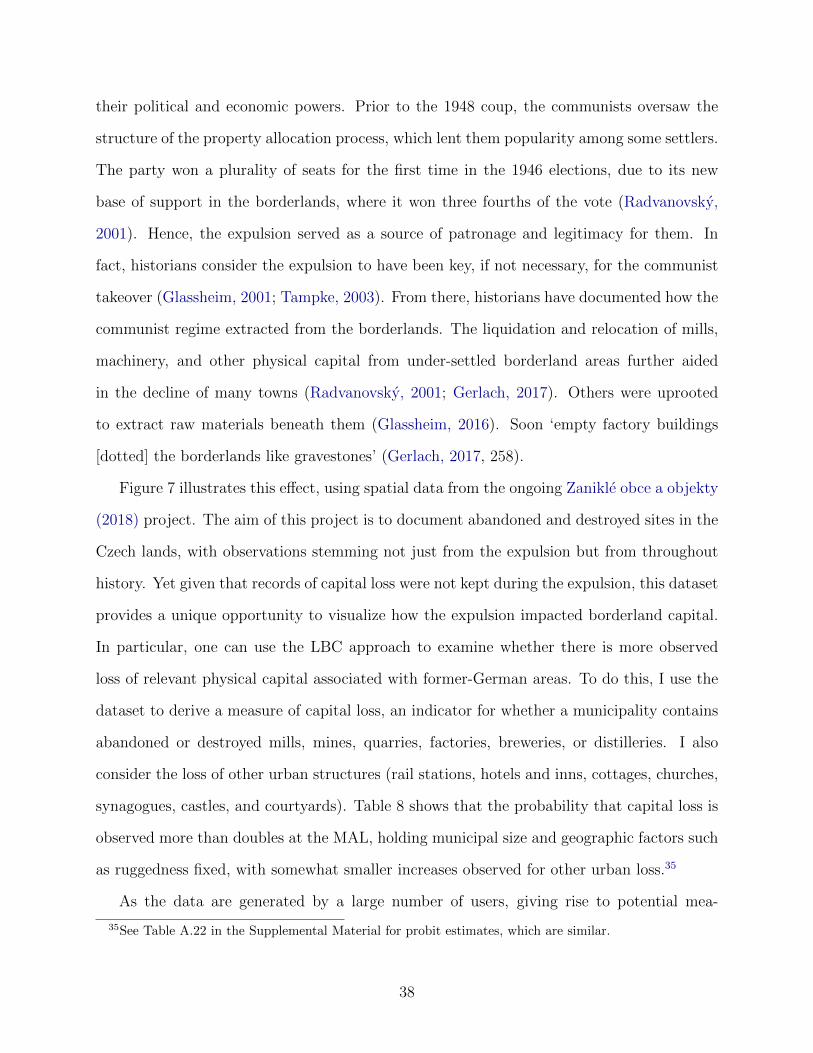
their political and economic powers. Prior to the 1948 coup, the communists oversaw the

structure of the property allocation process, which lent them popularity among some settlers.

The party won a plurality of seats for the first time in the 1946 elections, due to its new

base of support in the borderlands, where it won three fourths of the vote (Radvanovsky,

2001). Hence, the expulsion served as a source of patronage and legitimacy for them. In

fact, historians consider the expulsion to have been key, if not necessary, for the communist

takeover (Glassheim, 2001; Tampke, 2003). From there, historians have documented how the

communist regime extracted from the borderlands. The liquidation and relocation of mills,

machinery, and other physical capital from under-settled borderland areas further aided

in the decline of many towns (Radvanovsky, 2001; Gerlach, 2017). Others were uprooted

to extract raw materials beneath them (Glassheim, 2016). Soon ‘empty factory buildings

[dotted] the borderlands like gravestones’ (Gerlach, 2017, 258).

Figure 7 illustrates this effect, using spatial data from the ongoing Zanikle obce a objekty

(2018) project. The aim of this project is to document abandoned and destroyed sites in the

Czech lands, with observations stemming not just from the expulsion but from throughout

history. Yet given that records of capital loss were not kept during the expulsion, this dataset

provides a unique opportunity to visualize how the expulsion impacted borderland capital.

In particular, one can use the LBC approach to examine whether there is more observed

loss of relevant physical capital associated with former-German areas. To do this, I use the

dataset to derive a measure of capital loss, an indicator for whether a municipality contains

abandoned or destroyed mills, mines, quarries, factories, breweries, or distilleries. I also

consider the loss of other urban structures (rail stations, hotels and inns, cottages, churches,

synagogues, castles, and courtyards). Table 8 shows that the probability that capital loss is

observed more than doubles at the MAL, holding municipal size and geographic factors such

as ruggedness fixed, with somewhat smaller increases observed for other urban loss.35

As the data are generated by a large number of users, giving rise to potential mea-

35See Table A.22 in the Supplemental Material for probit estimates, which are similar.

38

Table 8: Observed Capital Loss

Capital loss Other urban loss(1a) (1b) (2a) (2b)

In borderlands .125 – .043 –(linear in distance) (.029)∗∗∗ (.022)∗

In borderlands – .130 – .077(linear in x and y) (.028)∗∗∗ (.018)∗∗∗

R2 .253 .256 .272 .269Mean dep. var. in interior .088 (.284) .068 (.252)Observations 4049 4049 4049 4049Clusters 71 71 71 71Border segments 50 50 50 50Bandwidth 25 km 25 km 25 km 25 km

Robust standard errors are clustered by district, with ***, **, and * denoting significance at the 1%, 5%, and 10% levels,respectively. Notes: All regressions exclude Prague and Polish Zaolzie, include border segment and district fixed effects aswell as exogenous controls for elevation, ruggedness, precipitation, temperature, and river density (km per km2), and utilizea local linear running variable of either distance from the Munich Agreement line interacted with the treatment or longitudeand latitude. I also control for municipal size (km2). Units of observation are municipalities. Capital loss indicates whether amunicipality has any observed abandoned or destroyed mills, mines, quarries, factories, breweries, or distilleries. Other urbanloss indicates whether a municipality has any observed abandoned or destroyed rail stations, hotels and inns, cottages, churches,synagogues, castles, or courtyards.

surement error and especially observational selection for areas with higher probabilities of

abandonment (i.e. the borderlands), these coefficients should be taken with caution. How-

ever, the presence of significant capital loss in the borderlands is corroborated by a large and

well-established historical literature (Radvanovsky, 2001; Glassheim, 2001; 2016; Gerlach,

2017). Nevertheless, other potential issues threaten the interpretation of such capital loss as

a causal channel. In particular, one important concern is that, rather than resulting from

the expulsion, some of the relative capital loss in Table 8 may actually have preceded it and

thus influenced the borderlands’ subsequent development independent of it.

For instance, Germany’s annexation of the borderlands during WWII would have left it

vulnerable to bombings by the Allied Powers. To address this, Figure A.3 in the Supple-

mental Material confirms bombings to be few and concentrated around major urban areas

regardless of region. At the same time, the end of WWII saw Czechoslovakia’s liberation

by Soviet and U.S. forces. Historical evidence suggests that some areas experienced a loss

of capital at that time. In particular, violent and appropriative behaviour was reported to

have taken place by Soviet Red Army soldiers (Gerlach, 2017). This might have hurt the

39

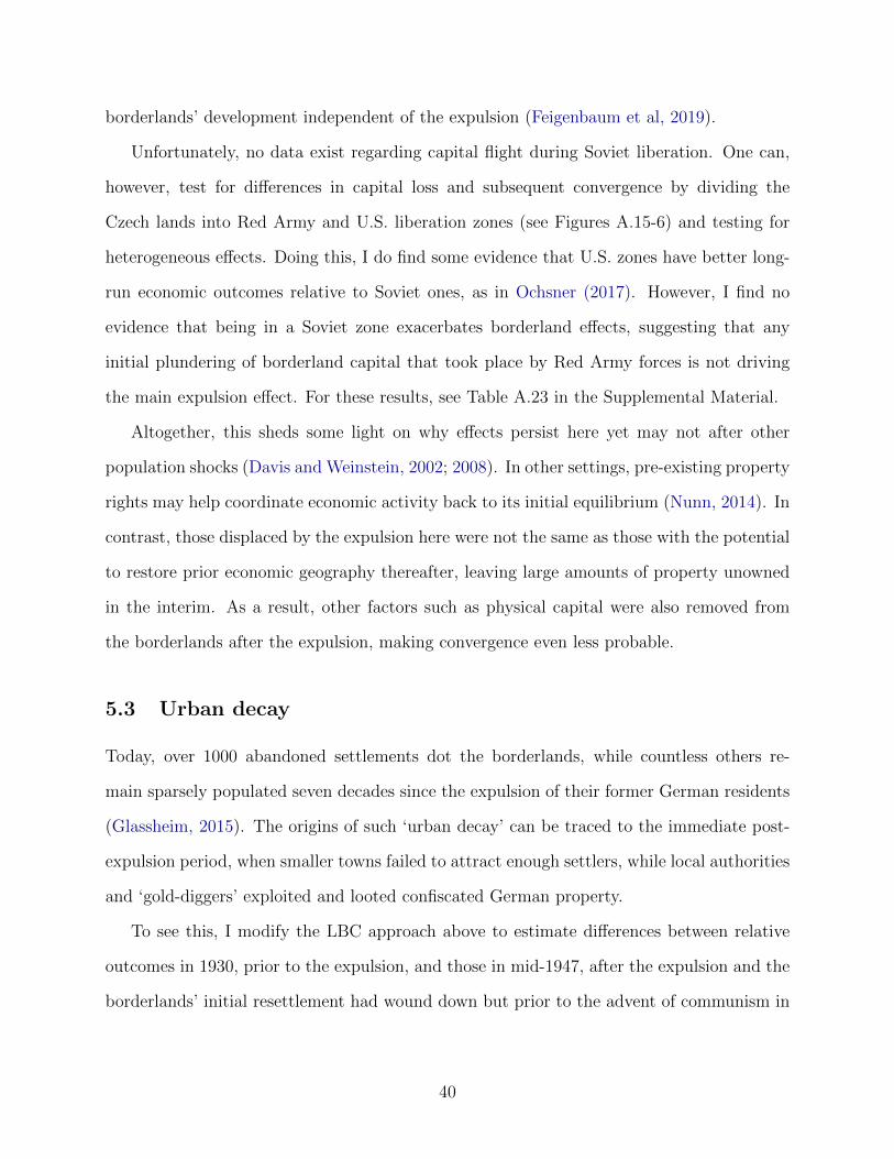
borderlands’ development independent of the expulsion (Feigenbaum et al, 2019).

Unfortunately, no data exist regarding capital flight during Soviet liberation. One can,

however, test for differences in capital loss and subsequent convergence by dividing the

Czech lands into Red Army and U.S. liberation zones (see Figures A.15-6) and testing for

heterogeneous effects. Doing this, I do find some evidence that U.S. zones have better long-

run economic outcomes relative to Soviet ones, as in Ochsner (2017). However, I find no

evidence that being in a Soviet zone exacerbates borderland effects, suggesting that any

initial plundering of borderland capital that took place by Red Army forces is not driving

the main expulsion effect. For these results, see Table A.23 in the Supplemental Material.

Altogether, this sheds some light on why effects persist here yet may not after other

population shocks (Davis and Weinstein, 2002; 2008). In other settings, pre-existing property

rights may help coordinate economic activity back to its initial equilibrium (Nunn, 2014). In

contrast, those displaced by the expulsion here were not the same as those with the potential

to restore prior economic geography thereafter, leaving large amounts of property unowned

in the interim. As a result, other factors such as physical capital were also removed from

the borderlands after the expulsion, making convergence even less probable.

5.3 Urban decay

Today, over 1000 abandoned settlements dot the borderlands, while countless others re-

main sparsely populated seven decades since the expulsion of their former German residents

(Glassheim, 2015). The origins of such ‘urban decay’ can be traced to the immediate post-

expulsion period, when smaller towns failed to attract enough settlers, while local authorities

and ‘gold-diggers’ exploited and looted confiscated German property.

To see this, I modify the LBC approach above to estimate differences between relative

outcomes in 1930, prior to the expulsion, and those in mid-1947, after the expulsion and the

borderlands’ initial resettlement had wound down but prior to the advent of communism in

40

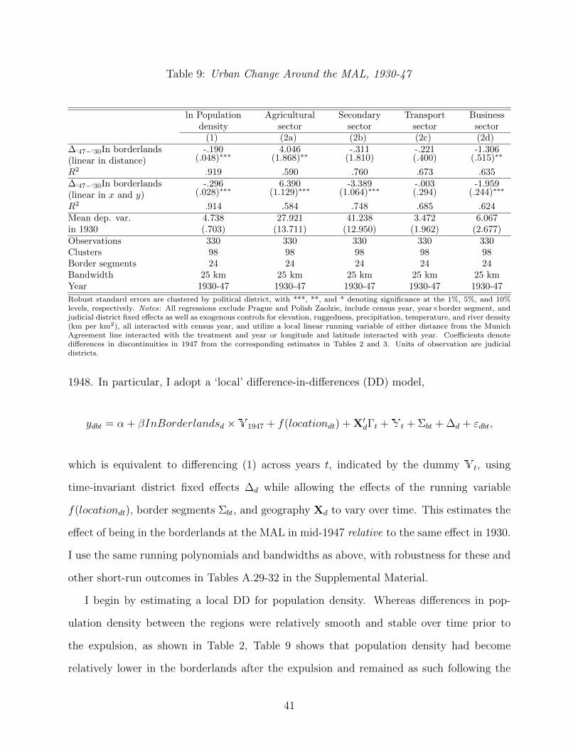
Table 9: Urban Change Around the MAL, 1930-47

ln Populationdensity

Agriculturalsector

Secondarysector

Transportsector

Businesssector

(1) (2a) (2b) (2c) (2d)∆‘47−‘30In borderlands -.190 4.046 -.311 -.221 -1.306(linear in distance) (.048)∗∗∗ (1.868)∗∗ (1.810) (.400) (.515)∗∗

R2 .919 .590 .760 .673 .635∆‘47−‘30In borderlands -.296 6.390 -3.389 -.003 -1.959(linear in x and y) (.028)∗∗∗ (1.129)∗∗∗ (1.064)∗∗∗ (.294) (.244)∗∗∗

R2 .914 .584 .748 .685 .624Mean dep. var. 4.738 27.921 41.238 3.472 6.067in 1930 (.703) (13.711) (12.950) (1.962) (2.677)Observations 330 330 330 330 330Clusters 98 98 98 98 98Border segments 24 24 24 24 24Bandwidth 25 km 25 km 25 km 25 km 25 kmYear 1930-47 1930-47 1930-47 1930-47 1930-47

Robust standard errors are clustered by political district, with ***, **, and * denoting significance at the 1%, 5%, and 10%levels, respectively. Notes: All regressions exclude Prague and Polish Zaolzie, include census year, year×border segment, andjudicial district fixed effects as well as exogenous controls for elevation, ruggedness, precipitation, temperature, and river density(km per km2), all interacted with census year, and utilize a local linear running variable of either distance from the MunichAgreement line interacted with the treatment and year or longitude and latitude interacted with year. Coefficients denotedifferences in discontinuities in 1947 from the corresponding estimates in Tables 2 and 3. Units of observation are judicialdistricts.

1948. In particular, I adopt a ‘local’ difference-in-differences (DD) model,

ydbt = α + βInBorderlandsd ×Y1947 + f(locationdt) + X′dΓt +Yt + Σbt + ∆d + εdbt,

which is equivalent to differencing (1) across years t, indicated by the dummy Yt, using

time-invariant district fixed effects ∆d while allowing the effects of the running variable

f(locationdt), border segments Σbt, and geography Xd to vary over time. This estimates the

effect of being in the borderlands at the MAL in mid-1947 relative to the same effect in 1930.

I use the same running polynomials and bandwidths as above, with robustness for these and

other short-run outcomes in Tables A.29-32 in the Supplemental Material.

I begin by estimating a local DD for population density. Whereas differences in pop-

ulation density between the regions were relatively smooth and stable over time prior to

the expulsion, as shown in Table 2, Table 9 shows that population density had become

relatively lower in the borderlands after the expulsion and remained as such following the

41

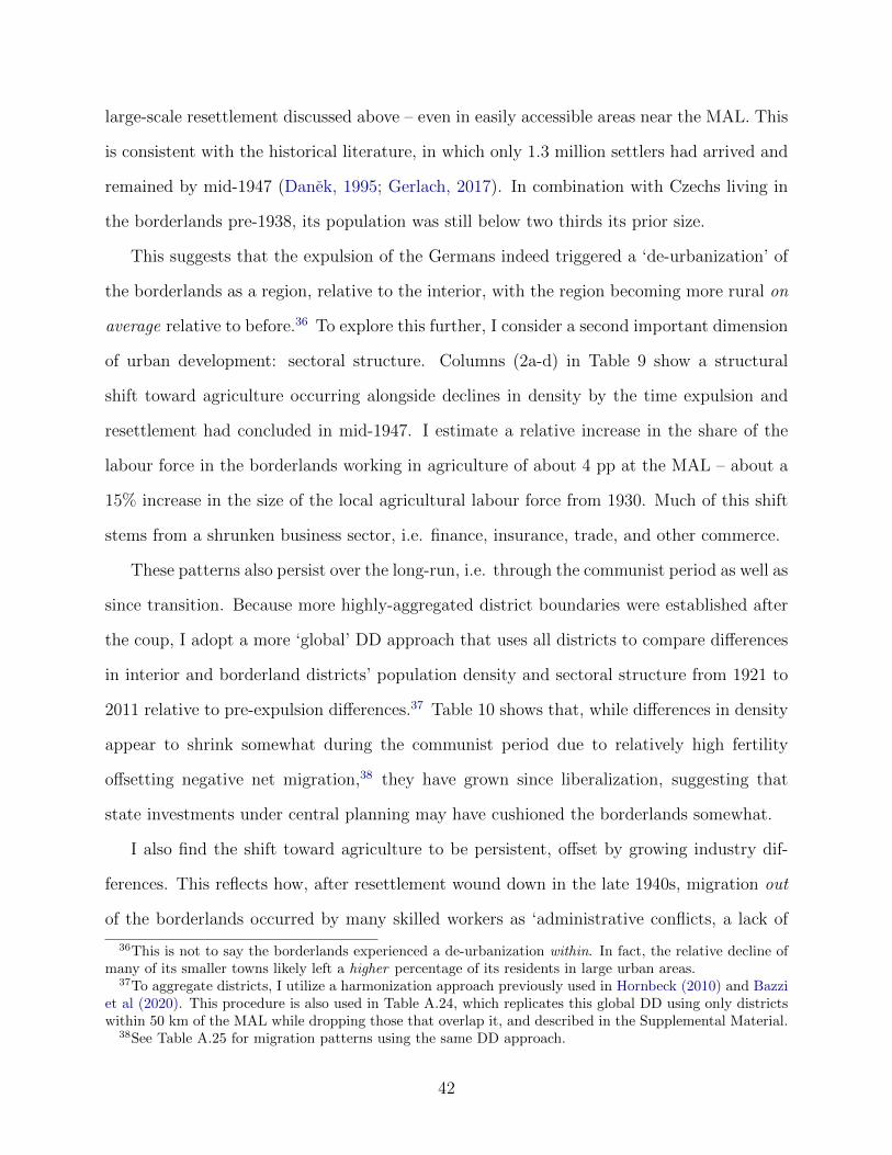
large-scale resettlement discussed above – even in easily accessible areas near the MAL. This

is consistent with the historical literature, in which only 1.3 million settlers had arrived and

remained by mid-1947 (Danek, 1995; Gerlach, 2017). In combination with Czechs living in

the borderlands pre-1938, its population was still below two thirds its prior size.

This suggests that the expulsion of the Germans indeed triggered a ‘de-urbanization’ of

the borderlands as a region, relative to the interior, with the region becoming more rural on

average relative to before.36 To explore this further, I consider a second important dimension

of urban development: sectoral structure. Columns (2a-d) in Table 9 show a structural

shift toward agriculture occurring alongside declines in density by the time expulsion and

resettlement had concluded in mid-1947. I estimate a relative increase in the share of the

labour force in the borderlands working in agriculture of about 4 pp at the MAL – about a

15% increase in the size of the local agricultural labour force from 1930. Much of this shift

stems from a shrunken business sector, i.e. finance, insurance, trade, and other commerce.

These patterns also persist over the long-run, i.e. through the communist period as well as

since transition. Because more highly-aggregated district boundaries were established after

the coup, I adopt a more ‘global’ DD approach that uses all districts to compare differences

in interior and borderland districts’ population density and sectoral structure from 1921 to

2011 relative to pre-expulsion differences.37 Table 10 shows that, while differences in density

appear to shrink somewhat during the communist period due to relatively high fertility

offsetting negative net migration,38 they have grown since liberalization, suggesting that

state investments under central planning may have cushioned the borderlands somewhat.

I also find the shift toward agriculture to be persistent, offset by growing industry dif-

ferences. This reflects how, after resettlement wound down in the late 1940s, migration out

of the borderlands occurred by many skilled workers as ‘administrative conflicts, a lack of

36This is not to say the borderlands experienced a de-urbanization within. In fact, the relative decline ofmany of its smaller towns likely left a higher percentage of its residents in large urban areas.

37To aggregate districts, I utilize a harmonization approach previously used in Hornbeck (2010) and Bazziet al (2020). This procedure is also used in Table A.24, which replicates this global DD using only districtswithin 50 km of the MAL while dropping those that overlap it, and described in the Supplemental Material.

38See Table A.25 for migration patterns using the same DD approach.

42

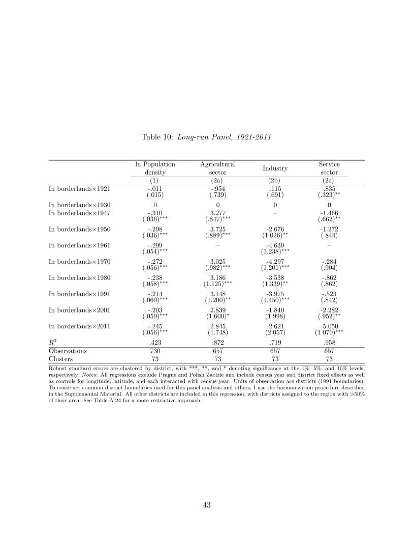
Table 10: Long-run Panel, 1921-2011

ln Populationdensity

Agriculturalsector

IndustryServicesector

(1) (2a) (2b) (2c)In borderlands×1921 -.011 -.954 .115 .835

(.015) (.739) (.691) (.323)∗∗

In borderlands×1930 0 0 0 0In borderlands×1947 -.310 3.277 – -1.466

(.036)∗∗∗ (.847)∗∗∗ (.662)∗∗

In borderlands×1950 -.298 3.725 -2.676 -1.272(.036)∗∗∗ (.889)∗∗∗ (1.026)∗∗ (.844)

In borderlands×1961 -.299 – -4.639 –(.054)∗∗∗ (1.238)∗∗∗

In borderlands×1970 -.272 3.025 -4.297 -.284(.056)∗∗∗ (.982)∗∗∗ (1.201)∗∗∗ (.904)

In borderlands×1980 -.238 3.186 -3.538 -.862(.058)∗∗∗ (1.125)∗∗∗ (1.339)∗∗ (.862)

In borderlands×1991 -.214 3.148 -3.975 -.523(.060)∗∗∗ (1.200)∗∗ (1.450)∗∗∗ (.842)

In borderlands×2001 -.203 2.839 -1.840 -2.282(.059)∗∗∗ (1.600)∗ (1.998) (.952)∗∗

In borderlands×2011 -.245 2.845 -2.621 -5.050(.056)∗∗∗ (1.748) (2.057) (1.070)∗∗∗

R2 .423 .872 .719 .958Observations 730 657 657 657Clusters 73 73 73 73

Robust standard errors are clustered by district, with ***, **, and * denoting significance at the 1%, 5%, and 10% levels,respectively. Notes: All regressions exclude Prague and Polish Zaolzie and include census year and district fixed effects as wellas controls for longitude, latitude, and each interacted with census year. Units of observation are districts (1991 boundaries).To construct common district boundaries used for this panel analysis and others, I use the harmonization procedure describedin the Supplemental Material. All other districts are included in this regression, with districts assigned to the region with >50%of their area. See Table A.24 for a more restrictive approach.

43

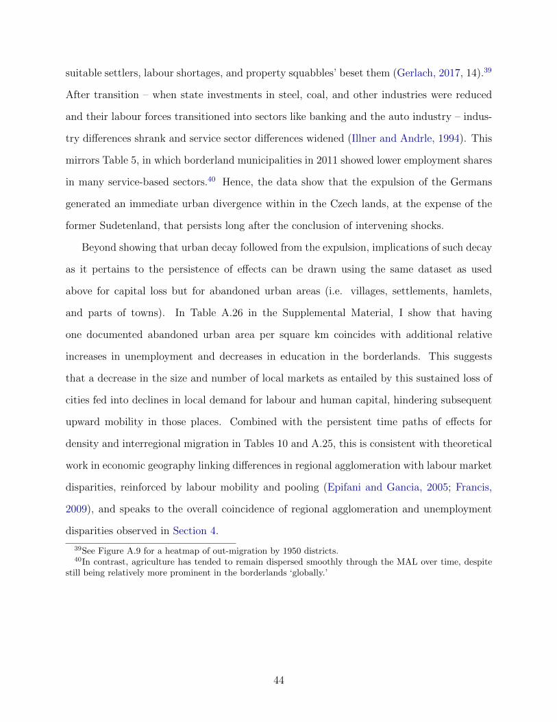
suitable settlers, labour shortages, and property squabbles’ beset them (Gerlach, 2017, 14).39

After transition – when state investments in steel, coal, and other industries were reduced

and their labour forces transitioned into sectors like banking and the auto industry – indus-

try differences shrank and service sector differences widened (Illner and Andrle, 1994). This

mirrors Table 5, in which borderland municipalities in 2011 showed lower employment shares

in many service-based sectors.40 Hence, the data show that the expulsion of the Germans

generated an immediate urban divergence within in the Czech lands, at the expense of the

former Sudetenland, that persists long after the conclusion of intervening shocks.

Beyond showing that urban decay followed from the expulsion, implications of such decay

as it pertains to the persistence of effects can be drawn using the same dataset as used

above for capital loss but for abandoned urban areas (i.e. villages, settlements, hamlets,

and parts of towns). In Table A.26 in the Supplemental Material, I show that having

one documented abandoned urban area per square km coincides with additional relative

increases in unemployment and decreases in education in the borderlands. This suggests

that a decrease in the size and number of local markets as entailed by this sustained loss of

cities fed into declines in local demand for labour and human capital, hindering subsequent

upward mobility in those places. Combined with the persistent time paths of effects for

density and interregional migration in Tables 10 and A.25, this is consistent with theoretical

work in economic geography linking differences in regional agglomeration with labour market

disparities, reinforced by labour mobility and pooling (Epifani and Gancia, 2005; Francis,

2009), and speaks to the overall coincidence of regional agglomeration and unemployment

disparities observed in Section 4.

39See Figure A.9 for a heatmap of out-migration by 1950 districts.40In contrast, agriculture has tended to remain dispersed smoothly through the MAL over time, despite

still being relatively more prominent in the borderlands ‘globally.’

44

Table 11: Short-run Educational Effects, Mid-1947

Primary & lower secondary Upper secondary TertiaryEnrollment,general5-14

Enrollment,civic10-14

Enrollment,agricultural15-19

Enrollment,vocational15-19

Enrollment,college15-24

(1a) (1b) (2a) (2b) (3)In borderlands 5.651 -8.204 7.174 -12.980 -2.926(linear in distance) (.967)∗∗∗ (2.661)∗∗∗ (1.817)∗∗∗ (5.15)∗∗ (.449)∗∗∗

R2 .867 .589 .485 .241 .734In borderlands 6.959 -7.669 5.562 -6.293 -2.574(linear in x and y) (.728)∗∗∗ (2.395)∗∗∗ (1.374)∗∗∗ (4.398) (.374)∗∗∗

R2 .86 .591 .517 .214 .724Mean dep. var. 52.694 57.142 5.762 17.031 3.215in interior (2.398) (5.513) (3.951) (11.208) (1.358)Observations 115 115 115 115 115Border segments 16 16 16 16 16Bandwidth 50 km 50 km 50 km 50 km 50 kmYear 1947 1947 1947 1947 1947

Robust standard errors reported in brackets, with ***, **, and * denoting significance at the 1%, 5%, and 10% levels, respectively.Notes: All regressions exclude Prague and Polish Zaolzie, include border segment fixed effects as well as exogenous controls forelevation, ruggedness, precipitation, temperature, and river density (km per km2), and utilize a local linear running variable ofeither distance from the Munich Agreement line interacted with the treatment or longitude and latitude. Units of observationare political districts. All outcomes represent enrollment in a given type of schooling as a share (out of 100) of the relevant agepopulation.

5.4 Regional human capital inequalities

Recall that there was little difference in average literacy around the MAL prior to the ex-

pulsion of the Germans. However, compositional changes associated with post-expulsion

migration and the borderlands’ subsequent urban decay may have generated differences in

human capital between the regions, making it relatively more concentrated in the interior.

This in turn could have fed back into sectoral change (Moretti, 2004), locking in human cap-

ital inequalities between the regions over the longer-run. Such a pattern would be consistent

with the historical narrative that settlers were disproportionately unskilled (Radvanovsky,

2001; Glassheim, 2016), as well as the finding that the borderlands is less educated today.

While no data exist on educational attainment for the postwar Czech lands until 1961,

some evidence that the borderlands already had lower human capital post-resettlement can

be found by examining regional school enrollment patterns in mid-1947, after the main waves

of expulsion and resettlement had wound down. Until the coup in 1948, Czechoslovakia had

8 years of compulsory education. For primary education, children attended a general school

45

(obecna skola) for 5 years. Following this, one could either complete his or her education

with 3 more years at a general school or pursue a more advanced lower secondary education.

Commonly, this entailed attending a civic school (mest’anska skola) for 3 years. This in turn

was a prerequisite for subsequent upper secondary (e.g. vocational) education.41

Upon examining differences in school enrollment in mid-1947 between the post-expulsion,

post-resettlement borderlands and nearby interior areas, I find that rates of enrollment in

general schools among the relevant age group were significantly higher in the borderlands.

Given that all primary school-age children were enrolled in general schools regardless of

region, this had to have been driven by differences at the lower secondary level – namely, a

greater share of 10-14 year olds in the borderlands forgoing civic schooling in favor of the

terminal general school track. Consistent with this, I find that civil school enrollment rates

among 10-14 year olds were significantly lower in the borderlands in mid-1947 relative to

those of nearby interior areas. This can be seen in Table 11.

This also means that there would have been relatively fewer students in the borderlands

going on to pursue more advanced education. Column (3) confirms strikingly lower rates of

college enrollment in the borderlands relative to the interior in mid-1947, about a 90% de-

crease from crossing the MAL. Yet there were also differences in the types of schooling being

pursued among advanced students. To show this, I examine enrollment data from mid-1947

for two common types of upper secondary schools: basic vocational schools (zakladnı odborna

skola) and agricultural folk schools (lidova skola zemedelska). The former provided education

specific to a variety of trades, while the latter were meant for those going into agriculture.

Examining these, I observe another striking trend, which mirrors the sectoral changes ob-

served above: while basic vocational schooling was significantly less popular among those

living in the borderlands in mid-1947 relative to those in nearby interior areas, enrollment

in agricultural folk schools among the relevant age group was >100% higher. This suggests

that even among those in the borderlands who did go on to pursue advanced education,

41For more, see Michalicka and Svojtkova (1972) and Greger et al (2012).

46

there was a tendency to invest in agricultural skills over other, more technical skills.

Overall, these findings are consistent with the notion that those who selected into the

borderlands after the expulsion of 3 million Germans had less demand for advanced and

technical education, relative to those who stayed in nearby interior areas. In contrast, I

do not find consistent evidence that these early patterns were driven by supply-side factors.

Table A.27 in the Supplemental Material shows that, while the borderlands’ civic schools may

have had slightly fewer teachers per pupil relative to nearby interior ones, its general and

agricultural schools exhibited similar shortages despite having higher relative enrollment,

while its vocational schools had greater teacher-pupil ratios on average. Moreover, the

college enrollment measure in Table 11 exclusively measures demand, insofar as the location

of college enrollment is not restricted to the district of observation in the data.

Hence, despite Germans and Czechs previously having similar levels of education, the

expulsion of the Germans generated a loss of human capital in former-German areas be-

ginning with compositional changes they endured during their resettlement. Of course, it

is difficult to discern to what extent this was driven by a lack of skilled workers selecting

into the borderlands versus fewer incentives to become skilled there due to a lack of skill-

intensive sectors. More than likely there was a feedback between the two, reinforced by more

permanent labour market changes. Consistent with this, long-run trends show alongside the

sectoral changes in Table 10 downturns in education that persist to today (see Table A.28).

Given similar changes in density, this is also consistent with recent theoretical and empiri-

cal work in economic geography, showing human capital spillovers to be an important force

driving urban and labour market density (Duranton and Puga, 2004; Moretti, 2004).

5.5 Additional channels

This paper shows a persistent spatial divergence in local development within the Czech lands

following the 1945 expulsion of 3 million Germans from its borderlands. It has also discussed

the origins of these patterns, which emerged immediately following the expulsion and persist

47

decades after. That being said, there may be other forces contributing to the persistence of

or variation in such differences. I now consider three additional channels.

Natural geography

The analysis thus far controls for locational fundamentals, with physical geography being

smooth through the MAL. Alternative specifications using only geographically cohesive (i.e.

flat through the MAL) parts of the sample yield similar long-run effects, as shown in Table

A.15 in the Supplemental Material. Yet strong locational fundamentals may nonetheless

have helped mitigate the expulsion’s long-run effects within the borderlands. Since access to

water may contribute to economic performance through improved agriculture or transport,

I expand the analysis by interacting the treatment variable (and running variable, where

applicable) with a mean-normalized river density control, which indicates km of waterways

per square km in each municipality. Estimates suggest a possible, albeit noisy, attenuation

effect from the presence of rivers on some long-run effects. These can be found in Table

A.33. I find minimal evidence of any such effect for ruggedness.

Central planning

The expulsion and the borderlands’ resettlement occurred prior to the communist coup of

1948, when Czechoslovakia’s labour economy still operated to a large extent via the market

mechanism (Bernasek, 1970). However, it is important to consider to what extent central-

planning institutions helped preserve this divergence post-1947. If signs of convergence are

observed as having occurred around the MAL since transition, then it might mean that this

persistence had more to do with active central-planning decisions, whereas local losses in

e.g. density may not have persisted to the same extent in a market economy.

To test this, I consider in Table A.34 trends in relevant outcomes between 2001 and 2011,

after the end of communism and the restructuring of the 1990s. Differences in density and

unemployment remain highly stable near the MAL. I find similar stability for sector shares,

48

although the construction sector declines somewhat more as a share of the labour force in the

borderlands relative to the interior in both specifications. Yet overall, and despite large-scale

structural change since transition, differences remain remarkably flat. This, combined with

the overall persistence of patterns during communism and through transition (e.g. those in

Table 10), downplays the importance of central-planning institutions. That being said, the

communist regime itself plays a key role here, as discussed in Section 5.2.

Market access and international relations

For various reasons, the borderlands was likely a less appealing place to live during the

Cold War: for instance, its proximity to West Germany and Austria (e.g. due to damaged

trade networks, as well as poor international relations and fear of expellee return), as well

as economic isolation associated with the Iron Curtain in places closer to Poland and East

Germany (Redding and Sturm, 2008). However, it is unclear whether such factors would

have mattered at the MAL, where borderland and interior areas were similarly distant from

the national border.

I begin by examining whether living in the borderlands ever entailed greater economic

isolation in areas near the MAL. To measure this, I look for differences in the density of

railways through the MAL in 1930, 1940, 1960, and today (Donaldson and Hornbeck, 2016).

I find no evidence of decreased market access in the borderlands relative to the interior in

any time period. Furthermore, upon comparing effects in areas closer to the Eastern Bloc

(East Germany and Poland) versus West Germany and Austria, I do not find smoothness to

vary across space.42 Note that this does not imply a lack of increased isolation closer to the

national border, where trade might be more limited in one direction. Indeed, one advantage

of my identification strategy is that borderland areas being studied are close to the interior

and often quite far from the national border. Hence, economic isolation does not seem to

be driving short- or long-run local effects, either overall or associated with e.g. the Iron

42See Figure A.17 in the Supplemental Material for these maps.

49

Curtain. These results can be found in Table A.35 in the Supplemental Material.

It is still possible that proximity to West Germany and Austria would have entailed other

economic disadvantages, given the tensions of the postwar era. For instance, after WWII, the

Czechoslovak government intentionally kept parts of the borderlands on the West German

border emptied as a military buffer zone (Illner and Andrle, 1994). Table A.36 shows several

of the baseline long-run regressions with an interaction term for whether a municipality was

closer to Eastern Bloc areas prior to 1989. I find no differential effects here either.

6 Discussion and conclusion

For centuries, Czech- and German-speaking peoples lived alongside each other, growing the

whole of the Czech lands into one of the most developed parts of Europe by the early 20th

century (Klein and Ogilvie, 2016). Yet the rise of nationalism and the events of WWII

changed that forever, culminating in the expulsion of 3 million Germans in 1945. This paper

documents how that event continues to influence the relative development of former-German

areas and economic geography of the Czech lands more than half a century later.

Though this analysis has focused extensively on how these effects emerged and persisted,

numerous questions inevitably remain. For instance, what role did communism play in

driving persistence relative to what would have persisted regardless? On one hand, the

persistence of effects through transition and the relative stability of trends around the former

German ‘language border’ today suggests that central planning was unnecessary ex post for

persistence. On the other hand, this paper documents how the communists extracted capital

and raw materials from the borderlands following its initial de-urbanization, as discussed in

Section 5. As such, it remains unclear how effects might have differed had Czechoslovakia

been more like Austria or Finland during the Cold War. Future work should delve deeper

into how this period of central planning matters for long-run effects (i.e. post-transition).

This would tell us more about both the channels of persistence in this particular setting, as

50

well as the extent to which policy can influence long-run development more generally.

Household-level data collection and analysis is also needed. This might entail examining

narrow areas around the former language border, as in Karaja and Rubin (2017), to better

understand the choice to resettle the borderlands as well as transmission mechanisms at play

at a more micro level.

Finally, external validity remains a concern in the literature on forced migration, as

expulsion and similar events often occur during wartime and in poorly institutionalized

settings. Given the continued importance of studying forced migration, future research

should examine and compare effects in a variety of institutional and historical settings,

including forced migration as a result of non-political factors such as climate change.

This paper provides several important lessons for understanding forced migration, at a

time when the number of forcibly displaced worldwide is about 80 million. First, it illustrates

how such events may affect not only targeted groups but also have long-term implications

for development and regional inequality within the origin economy. Moreover, it shows that

forced migration can have strong and persistent effects even when compositional factors such

as human capital are similar across treated and control areas. This is no trivial insight. While

previous research has focused on expulsions involving relatively high-skilled minorities, forced

migration has plagued groups from many backgrounds throughout history. This should give

political leaders pause when considering the displacement of any minority group, as doing

so may leave a lasting mark on the places left behind.

51

References

[1] Abramitzky, R., Boustan, L. P. and Eriksson, K. (2014). ‘A nation of immigrants: assimilationand economic outcomes in the Age of Mass Migration,’ Journal of Political Economy, vol.122(3), pp. 467-506.

[2] Acemoglu, D. and Dell, M. (2010). ‘Productivity differences between and within countries,’American Economic Journal: Macroeconomics, vol. 2(1), pp. 169-88.

[3] Acemoglu, D., Johnson, S. and Robinson, J.A. (2002). ‘Reversal of fortune: geography andinstitutions in the making of the modern world income distribution,’ Quarterly Journal ofEconomics, vol. 117(4), pp. 1231-94.

[4] Acemoglu, D., Hassan, T. A. and Robinson, J. A. (2011). ‘Social structure and development:a legacy of the Holocaust in Russia,’ Quarterly Journal of Economics, vol. 126(2), pp. 895-946.

[5] Agnew, H. (2004). The Czechs and the Lands of the Bohemian Crown. Stanford: HooverInstitution Press.

[6] Akbulut-Yuksel, M. and Yuksel, M. (2015). ‘The long-term direct and external effects ofJewish expulsion in Nazi Germany,’ American Economic Journal: Economic Policy, vol. 7(3),pp. 58-85.

[7] Allen, T. and Donaldson, D. (2018). “The geography of path dependence.” Working Paper,Stanford University.

[8] Amtliches Deutsches Ortsbuch fur das Protektorat Bohmen und Mahren (1940). Prague: Re-ichsprotektor in Bohmen und Mahren.

[9] Arbatli, C. E. and Gokmen, G. (2019). “Ethnic capital and sub-national development: Ar-menian and Greek legacy in post-expulsion Turkey.” Working Paper, CESifo Working PaperSeries.

[10] von Arburg, A. (2001). Die Besiedlung der Grenzgebiete der bohmischen Lander 1945-1950.Vienna: University of Vienna.

[11] ARCDATA PRAHA (2017). https://www.arcdata.cz/ (last accessed: 2 August 2020).

[12] Armstrong, H. F. (1939). ‘Armistice at Munich,’ Foreign Affairs, vol. 17(2), pp. 197-290.

[13] Bach, T. (1923). ‘Education in Czechoslovakia,’ Department of the Interior Bureau of Educa-tion, Bulletin, 1922, No. 39, pp. 1-26.

[14] Bauer, T. K., Braun, S. T. and Kvasnicka, M. (2013). ‘The economic integration of forcedmigrants: evidence for postwar Germany,’ Economic Journal, vol. 123(571), pp. 998-1024.

[15] Bazzi, S., Fiszbein, M. and Gebresilasse, M. (2020). ‘Frontier culture: the roots and persistenceof ‘rugged individualism’ in the United States,’ Econometrica. Forthcoming.

[16] Becker, S. O. and Ferrara, A. (2019). ‘Consequences of forced migration: a survey of recentfindings,’ Labour Economics, vol. 59(C), pp. 1-16.

52

[17] Becker, S. O., Grosfeld, I., Grosjean, P., Voigtlander, N. and Zhuravskaya, E. (2020). ‘Forcedmigration and human capital: evidence from post-WWII population transfers,’ AmericanEconomic Review, vol. 110(5), pp. 1430-63.

[18] Bell, B., Fasani, F. and Machin, S. (2013). ‘Crime and immigration: evidence from largeimmigrant waves.’ Review of Economics and Statistics, vol. 21(3), pp. 1278-90.

[19] Bernasek, M. (1970). ‘Czechoslovak planning, 1945-48,’ Soviet Studies, vol. 22(1), pp. 94-109.

[20] Bleakley, H. and Lin, J. (2012). ‘Portage and path dependence,’ Quarterly Journal of Eco-nomics, vol. 127(2), pp. 587-644.

[21] Bosker, M., Brakman, S., Garretsen, H. and Schramm, M. (2007). ‘Looking for multipleequilibria when geography matters: German city growth and the WWII shock,’ Journal ofUrban Economics, vol. 61(1), pp. 152-67.

[22] Braun, S. T., Kramer, A., Kvasnicka, M. and Meier, P. (2020). ‘Local labour markets and thepersistence of population shocks: evidence from West Germany, 1939-70,’ Journal of EconomicGeography. Forthcoming.

[23] Bryant, C. (2002). ‘Either German or Czech: Fixing nationality in Bohemia and Moravia,1939-1946,’ Slavic Review, vol. 61(4), vol. 683-706.

[24] – (2007). Prague in Black: Nazi Rule and Czech Nationalism. London: Harvard UniversityPress.

[25] Chaney, E. and Hornbeck, R. (2016). ‘Economic dynamics in the Malthusian era: evidencefrom the 1609 Spanish expulsion of the Moriscos,’ Economic Journal, vol. 126(594), pp. 1404-40.

[26] Conley, T. (1999). ‘GMM estimation with cross sectional dependence,’ Journal of Economet-rics, vol. 92(1), pp. 1-45.

[27] Cornwall, M. (1994). ‘The struggle on the Czech-German language border, 1880-1940,’ EnglishHistorical Review, vol. 109(433), pp. 914-51.

[28] Danek, P. (1995). ‘Towards cultural regionalization of the Czech lands: Sudeten half a centuryafter the transfer,’ Geography, vol. 1995(25), pp. 41-60.

[29] Davis, D. R. and Weinstein, D. E. (2002). ‘Bones, bombs, and break points: the geography ofeconomic activity,’ American Economic Review, vol. 92(5), pp. 1269-89.

[30] – (2008). ‘A search for multiple equilibria in urban industrial structure,’ Journal of RegionalScience, vol. 48(1), pp. 29-65.

[31] Dell, M. (2010). ‘The persistent effects of Peru’s mining mita,’ Econometrica, vol. 78(6), pp.1863-1903.

[32] Dell, M. and Olken, B. A. (2019). ‘The development effects of the extractive colonial economy:the Dutch Cultivation System in Java,’ Review of Economic Studies, vol. 87, pp. 164-203.

[33] Donaldson, D. and Hornbeck, R. (2016). ‘Railroads and American economic growth: a ‘marketaccess’ approach,’ Quarterly Journal of Economics, vol. 131(2), pp. 799-858.

53

[34] Droller, F. (2017). ‘Migration, population composition, and long-run economic development:evidence from settlements in the Pampas,’ Economic Journal, vol. 127(614), pp. 1-32.

[35] Duranton, G. and Puga, D. (2004). “Micro-foundations of urban agglomeration economies,Handbook of Regional and Urban Economics, eds. J. V. Henderson and J. Thisse, vol. 4, pp.2063-117, New York: North Holland.

[36] Epifani, P. and Gancia, G. A. (2005). ‘Trade, migration, and regional unemployment,’ RegionalScience and Urban Economics, vol. 35(6), pp. 625-44.

[37] Erlikhman, V. (2004). Poteri Narodonaseleniia v XX Veke: Spravochnik, Moscow: RusskaiaPanorama.

[38] Eugster, B., Lalive, R., Steinhauer, A. and Zweimuller, J. (2017). ‘Culture, work attitudes,and job search: evidence from the Swiss language border,’ Journal of European EconomicAssociation, vol. 15(5), pp. 1056-1100.

[39] Feigenbaum, J. J., Lee, J., and Mezzanotti, F. (2019). ‘Capital destruction and economicgrowth: the effects of Sherman’s March, 1850-1920,’ Working Paper, NBER.

[40] Foged, M. and Peri, G. (2016). ‘Immigrants’ effect on native workers: new analysis on longi-tudinal data,’ American Economic Journal: Applied Economics, vol. 8(2), pp. 1-34.

[41] Francis, J. (2009). ‘Agglomeration, job flows and unemployment,’ Annals of Regional Science,vol. 43(1), pp. 181-98.

[42] Gelman, A. and Imbens, G. (2018). ‘Why high-order polynomials should not be used in re-gression discontinuity designs,’ Journal of Business and Economic Statistics, vol. 37(3), pp.447-56.

[43] Gerlach, D. (2017). The Economy of Ethnic Cleansing: The Transformation of the German-Czech Borderlands after WWII. New York: Cambridge University Press.

[44] Glassheim, E. (2001). ‘The mechanics of ethnic cleansing: the expulsion of Germans fromCzechoslovakia, 1945-47,’ Redrawing Nations: Ethnic Cleansing in East-Central Europe, eds.P. Ther and A. Siljak, pp. 197-219, Lanham, MD: Rowman & Littlefield.

[45] – (2015). ‘Unsettled landscapes: Czech and German conceptions of social and ecological declinein the postwar Czechoslovak borderlands,’ Journal of Contemporary History, vol. 50(2), pp.318-36.

[46] – (2016). Cleansing the Czechoslovak Borderlands: Migration, Environment, and Health in theFormer Sudetenland. Pittsburgh: University of Pittsburgh Press.

[47] Goldstein, E. (1999). ‘Neville Chamberlain, the British official mind and the Munich crisis,’Diplomacy & Statecraft, vol. 10(2-3), pp. 276-92.

[48] Greger D., Levınska, M. and Smetackova, I. (2012). ‘Priority education policies in the CzechRepublic: redesigning equity policies in the post-communist transformation,’ Educational Poli-cies and Inequalities in Europe, eds. M. Demeuse, D. Frandji, D. Greger, and J.Y. Rochex,London: Palgrave Macmillan.

54

[49] Grosfeld, I., Rodnyansky, A. and Zhuravskaya, E. (2013). ‘Persistent antimarket culture: alegacy of the Pale of Settlement after the Holocaust,’ American Economic Journal: EconomicPolicy, vol. 5(3), pp. 189-226.

[50] Guzi, M., Huber, P. and Mikula, S. (2019). ‘Old sins cast long shadows: the long term impactof the resettlement of the Sudetenland on residential migration,’ Working Paper, IZA.

[51] HGISe (2020). http://europa.udl.cat (last accessed: 2 August 2020).

[52] Hornbeck, R. (2010). ‘Barbed wire: property rights and agricultural development,’ QuarterlyJournal of Economics, vol. 125(2), pp. 767-810.

[53] Hornung, E. (2014). ‘Immigration and the diffusion of technology: the Huguenot diaspora inPrussia,’ American Economic Review, vol. 104(1), pp. 84-122.

[54] Hsiang, S. M. (2010). ‘Temperatures and cyclones strongly associated with economic produc-tion in the Caribbean and Central America,’ Proceedings of the National Academy of Sciences,vol. 107(35), pp. 15367-72.

[55] Illner, M. and Andrle, A. (1994). ‘The regional aspect of post-communist transformation inthe Czech Republic,’ Czech Sociological Review, vol. 2(1), pp. 107-27.

[56] Jedwab, R. and Moradi, A. (2016). ‘The permanent effects of transportation revolutions inpoor countries: evidence from Africa,’ Review of Economics and Statistics, vol. 98(2), pp.268-84.

[57] Jedwab, R., Johnson, N. and Koyama, M. (2019). ‘Pandemics, places, and populations: theeffects of the Black Death on urban development.’ Working Paper, Centre for Economic PolicyResearch.

[58] Johnson, N. D. and Koyama, M. (2017). ‘Jewish communities and city growth in preindustrialEurope,’ Journal of Development Economics, vol. 127(C), pp. 339-54.

[59] Jelınek, J. (2011). Analyza Topografickych Map 1:50000 z Obdobı Protektoratu Cechy aMorava. Bachelor thesis, Masaryk University. Masaryk University Information System.

[60] Judson, P. M. (2006). Guardians of the Nation: Activists on the Language Frontiers of ImperialAustria. Cambridge: Harvard University Press.

[61] Karaja, E. and Rubin, J. (2017). ‘The cultural transmission of trust norms: evidence from alab in the field on a natural experiment.’ Working Paper, Chapman University

[62] King, J. (2002). Budweisers into Czechs and Germans: A Local History of Bohemian Politics,1848-1948. Princeton: Princeton University Press.

[63] Klein, A. and Ogilvie, S. (2016). ‘Occupational structure in the Czech lands under the secondserfdom,’ Economic History Review, vol. 69(2), pp. 493-521.

[64] Kline, P. and Moretti, E. (2014). ‘Local economic development, agglomeration economies, andthe big push: 100 years of evidence from the Tennessee Valley Authority,’ Quarterly Journalof Economics, vol. 129(1), pp. 275-331.

55

[65] Korbel, J. (1959). The Communist Subversion of Czechoslovakia, 1938-1948. Princeton, NJ:Princeton.

[66] Krugman, P. (1991). ‘Increasing returns and economic geography,’ Journal of Political Econ-omy, vol. 99(3), pp. 483-99.

[67] Lee, D. S. and Lemieux, T. (2010). ‘Regression discontinuity designs in economics,’ Journalof Economic Literature, vol. 48(2), pp. 281-355.

[68] Maier, S. (2006). Das Grenzdurchgangslager Furth im Wald 1946-57, Stamsried: Vogel.

[69] Maloney, W. F. and Caicedo, F. V. (2015). ‘The persistence of (subnational) fortune,’ Eco-nomic Journal, vol. 126(598), pp. 2363-401.

[70] ‘Mapa o stavu vozovek Ceskoslovenskych silnic. 1. dıl, Zeme Ceska a Moravskoslezska.1:650 000.’ (1930). Prague: Autoklub RCS. https://digitool.is.cuni.cz/R/?func=

dbin-jump-full&object_id=1168737 (last accessed: 2 August 2020).

[71] Michalicka, M. and Svojtkova, V. (1972). Rozvoj Ceskoslovenskeho vseobecne vzdelavacıhoa odborneho skolstvı v letech 1945-1970. Prague: Pedagogicky ustav J.A. Komenskeho(Ceskoslovenska akademie ved).

[72] Michalopoulos, S. and Papaioannou, E. (2013). ‘Precolonial ethnic institutions and contem-porary African development,’ Econometrica, vol. 81(1), pp. 113-52.

[73] Moretti, E. (2004). ‘Human capital externalities in cities,’ Handbook of Regional and UrbanEconomics, eds. J. V. Henderson and J. Thisse, vol. 4, pp. 2243-91, New York: North Holland.

[74] Moscona, J., Nunn, N. and Robinson, J. A. (2020). ‘Segmentary lineage organization andconflict in Sub-Saharan Africa,’ Econometrica. Forthcoming.

[75] Murard, E. and Sakalli, S. O. (2019). ‘Mass refugee inflow and long-run prosperity: lessonsfrom the Greek population resettlement.’ Working Paper, IZA.

[76] Nunn, N. (2008). ‘The long-term effects of Africa’s slave trades,’ Quarterly Journal of Eco-nomics, vol. 123(1), pp. 139-76.

[77] – (2014). ‘Historical Development,’ Handbook of Economic Growth, eds. P. Aghion, and S. N.Durlauf, vol. 2A, pp. 347-402, Amsterdam, Netherlands: Elsevier North Holland.

[78] Ochsner, C. (2017). ‘Dismantled once, diverged forever? A quasi-natural experiment of RedArmy misdeeds in post-WWII Europe.’ Working Paper, ifo Working Paper Series.

[79] Odsun: Die Vertreibung der Sudetendeutschen (1995). Munich: Sudetendeutsches Archiv.

[80] OECD (2006). OECD Economic Surveys: Czech Republic 2006. Paris: OECD Publishing.

[81] ‘Osıdlenı pohranicı v letech 1945-1952’ (1953). Zpravy a rozbory, Praha: Statnı urad stati-sticky.

[82] Overmans, R. (2004). Deutsche Militarische Verluste im Zweiten Weltkrieg, Munich: Olden-bourg.

56

[83] Pascali, L. (2016). ‘Banks and development: Jewish communities in the Italian Renaissanceand current economic performance,’ Review of Economics and Statistics. 98(1):140-58.

[84] Peters, M. (2019). ‘Market size and spatial growth: evidence from Germany’s postwar popu-lation expulsions.’ Working Paper, Columbia University.

[85] Puga, D. (1999). ‘The rise and fall of regional inequalities,’ European Economic Review, vol.43(2), pp. 303-334.

[86] Radvanovsky, Z. (2001). ‘The social and economic consequences of resettling Czechs intoNorthwestern Bohemia, 1945-47,’ Redrawing Nations: Ethnic Cleansing in East-Central Eu-rope, eds. P. Ther and A. Siljak, pp. 241-60, Lanham, MD: Rowman & Littlefield.

[87] Redding, S. J. and Sturm, D. M. (2008). ‘The costs of remoteness: evidence from Germandivision and reunification,’ American Economic Review, vol. 98(5), pp. 1766-97.

[88] Redding, S. J., Sturm, D. M. and Wolf, N. (2011). ‘History and industry location: evidencefrom German airports,’ Review of Economics and Statistics, vol. 93(3), pp. 814-31.

[89] Rocha, R., Ferraz, C. and Soares, R. R. (2017). ‘Human capital persistence and development,’American Economic Journal: Applied Economics, vol. 9(4), pp. 105-36.

[90] Ruiz, I. and C. Vargas-Silva (2013). ‘The economics of forced migration,’ Journal of Develop-ment Studies, vol. 49(6), pp. 772-84.

[91] Schumann, A. (2014). ‘Persistence of population shocks: evidence from the occupation ofWest Germany after WWII,’ American Economic Journal: Applied Economics, vol. 6(3), pp.189-205.

[92] Semrad, A. (2015). ‘Immigration and educational spillovers: evidence from Sudeten Germanexpellees in post-war Bavaria.’ Working Paper, Munich Discussion Paper.

[93] Sequeira, S., Nunn, N. and Qian, N. (2019). ‘Immigrants and the making of America,’ Reviewof Economic Studies, vol. 87(1), pp. 382-419.

[94] Slomkova, V. (2016). Deti a valka: rok 1945 ve vzpomınkach pametnıku z Berounska aPlzenska. Thesis, Charles University. Charles University Digital Repository.

[95] Spurny, M. (2013). ‘Reliability and the border: the discourse of the Czech borderlands, 1945-49,’ Austrian Journal of Political Science, vol. 42(1), pp. 83-94.

[96] Sudetendeutsches Ortsnamenverzeichnis: Amtliches Gemeinde- und Ortsnamenverzeichnisder nach dem Munchener Abkommen vom 29. 9. 1938 (Grenzfestlegung vom 20.11.1938) zumDeutschen Reich gekommenen sudetendeutschen Gebiete. (1987). Munich: SudetendeutschesArchiv.

[97] Tabellini, G. (2010). ‘Culture and institutions: economic development in the regions of Eu-rope,’ Journal of the European Economic Association, vol. 8(4), pp. 677-716.

[98] Tampke, J. (2003). Czech-German Relations and the Politics of Central Europe. New York:Palgrave Macmillan.

57

[99] Testa, P. A. (2020). ‘Shocks and the spatial distribution of economic activity: the role ofinstitutions,’ Journal of Economic Behavior & Organization, Forthcoming.

[100] Theater History of Operations Reports (THOR) (2019). https://data.world/datamil/

world-war-ii-thor-data (last accessed: 3 August 2020).

[101] United Nations High Commissioner for Refugees (2019). https://www.unhcr.org/

globaltrends2019/ (last accessed: 3 August 2020).

[102] URRlab (2017). http://www.urrlab.cz/ (last accessed: 2 August 2020).

[103] U.S. Congress, House of Representatives, Committee of Foreign Affairs (1947). BackgroundInformation on European Countries: Political Conditions and Economic Recovery Problems.Washington D.C.: U.S. Government Printing Office.

[104] U.S. Department of State Office of the Historian (1945). ‘Document 450: The Ambassador inFrance (Caffery) to the Secretary of State,’ Foreign Relations of the United States: Diplo-matic Papers. Europe, Volume IV. https://history.state.gov/historicaldocuments/

frus1945v04/d450 (last accessed: 2 August 2020).

[105] Waldinger, F. (2010). ‘Quality matters: the expulsion of professors and the consequencesfor PhD student outcomes in Nazi Germany,’ Journal of Political Economy, vol. 118(4), pp.787-831.

[106] Wiedemann, A. (2016). ‘Pojd s Nami Budovat Pohranicı!’: Osıdlovanı a Promena Obyvatel-stva Byvalych Sudet 1945–1952. Prague: Proster.

[107] Winkler, E. (1936). ‘Nationalitatenkarte der Sudetenlander (Bohmen, Mahren-Schlesien),1:750,000.’ Karlsbad-Leipzig: Karl H. Frank.

[108] Wiskemann, E. (1938). Czechs and Germans: A Study of the Struggle in the HistoricProvinces of Bohemia and Moravia. London: Oxford University Press.

[109] Zahra, T. (2008). Kidnapped Souls: National Indifference and the Battle for Children in theBohemian Lands, 1900-48. Ithaca: Cornell University Press.

[110] Zanikle obce a objekty (2018). http://zanikleobce.cz/ (last accessed: 3 August 2020).

[111] de Zayas, A. (1989). A Terrible Revenge: The Ethnic Cleansing of the East European Ger-mans, 1944-50. New York: St. Martin’s Press.

58