THE ECONOMIC IMPACTS OF INCOME LEVEL, INTEREST

RATE, AND HOUSING PRICE ON HOUSEHOLD SAVING

BEHAVIOUR IN MALAYSIA

Lou Kah Lock

Bachelor of Economics with Honours

(International Economics)

2015

THE ECONOMIC IMPACTS OF INCOME LEVEL,

INTEREST RATE, AND HOUSING PRICE ON HOUSEHOLD SAVING

BEHAVIOUR IN MALAYSIA

LOU KAH LOCK

(36797)

This Project is submitted in partial fulfilment of

the requirements for the degree of Bachelor of Economics with Honours

(International Economics)

Faculty of Economics and Business

UNIVERSITI MALAYSIA SARAWAK

2015

iii

Statement of Originality

The work described in this Final Year Project, entitled

“THE ECONOMIC IMPACTS OF INCOME LEVEL, INTEREST RATE, AND

HOUSING PRICE ON HOUSEHOLD SAVING BEHAVIOUR IN MALAYSIA”

Is to the best of the author’s knowledge that of the author except where due

reference is made.

(Date submitted ) (Student’s signature)

Full Name

Matric number

iv

ACKNOWLEDGEMENTS

First of all, I would like to express my gratitude to my supervisor, Mr. Dzul Hadzwan

Husaini, for his guidance throughout this study which in terms of advices, comments, and

suggestions.

Besides, I am also like to thank for other lecturers in the Faculty of Economics and

Business who always generous sharing their knowledge and giving encouragement to me.

Lastly, I am very grateful to my family members and friends who always support me

along the process of finishing this research paper.

Again, thank you to all of you.

v

LIST OF TABLES

PAGE

Table 2.3: Summary of Literature Review 27-36

Table 4.1: ADF unit root and stationarity test 61

Table 4.2: Cointegration Test and Hypothesis Testing 63

Table 4.3: Normalizing cointegrating coefficients 63

Table 4.4: VECM granger causality test 66

Table 4.5: White’s general heteroscedasticity test 69

Table 4.6: Generalized Variance Decompositions (GVDCs) 72

vi

LIST OF FIGURES

PAGE

Figure 1.1: Household saving ratio of Malaysia 6

Figure 1.2: Malaysia’s Personal disposable income (constant) 7

Figure 1.3: Saving, lending, and interest rates of Malaysia 9

Figure 1.4: Classification of loans by purpose in Malaysia 11

Figure 1.5: House price index of Malaysia 12

Figure 4.1: Logarithm of real household savings 57

Figure 4.2: Logarithm of real personal disposable income 57

Figure 4.3: Logarithm of house price index 58

Figure 4.4: Saving rate 58

Figure 4.5: Short Run Causality Direction 66

Figure 4.6: CUSUM test 68

Figure 4.7: CUSUM of Squares test 68

Figure 4.8: Generalized Impulse Response Function (IRFs) 75

vii

ABSTRACT

THE ECONOMIC IMPACTS OF INCOME LEVEL, INTEREST RATE, AND

HOUSING PRICE ON HOUSEHOLD SAVING BEHAVIOUR IN MALAYSIA

By

Lou Kah Lock

The purpose of this study is to examine the long run and short run relationships

between interest rate, income level, housing price, and household saving in Malaysia. The

data set included in this study are saving rate, real personal disposable income, housing

price index, and real household saving in Malaysia. Observation of these quarterly time

series data are 44, where started from first quarter of 2001 until fourth quarter of 2011.

Based on the Absolute Income Hypothesis (AIH) that suggested by Burney and Khan

(1992), a model with household saving as dependent variable and interest rate, income

level, and housing price as independent variables are able to be constructed. There are

several economic procedures employed in this study to test this model, which are ADF

unit root test, Johansen and Juselius cointegration test, VECM granger causality test,

CUSUM and CUSUM of squares tests, White heteroscedasticity test, generalized

variance decompositions test, and generalized impulse response functions test. The result

of JJ cointegration test suggesting that these four-dimensional system do not move apart

and sharing one long run relationship in the long run. It enable VECM granger causality

viii

test being employed in this study to examine the long run and short run relationships of

these four time series variables.

In the long run, the ECT in the VECM model suggesting that housing price index

able to receive the shocks from other variables and make 3.20% of adjustment in the short

run in order to achieve long run equilibrium. The time taken for housing price to reach

equilibrium is quite long, where approximately 31.25 quarters. In the short run, all of the

independent variables able to cause household saving directly except housing price index.

Housing price index can only cause household saving indirectly by influencing the

personal disposable income. This result able to be explained by the wealth effect of

appreciation or depreciation in housing price. According to Koskela et al. (1992), higher

housing price will increase the implicit value of wealth among the house owner and thus

increase the real value of personal disposable income, induce higher money spending, and

resulted low saving. Besides, interest rate also able to affect household saving indirectly

by bringing wealth effect to the personal disposable income.

The findings from this study highlighted interest rate and housing price can be the

tools to adjust household saving in the short run but as the time goes on, housing price

will be getting affected. Thus, it is suggesting policy makers should have deep

consideration to adjust the housing price and interest rate in order to achieve expected

level of consumption and saving in Malaysia.

ix

ABSTRAK

KESAN-KESAN TAHAP PENDAPATAN, KADAR FAEDAH DAN HARGA

RUMAH TERHADAP GELAGAT TABUNG ISI RUMAH DI MALAYSIA

Oleh

Lou Kah Lock

Tujuan kajian ini dijalankan adalah untuk mengkaji hubungan jangka panjang dan

jangka pendek di antara kadar faedah, tahap pendapatan, harga rumah, dan tabungan isi

rumah di Malaysia. Data dalam kajian ini adalah merangkumi kadar faedah, pendapatan

boleh guna benar isi rumah, indeks harga rumah, dan tabung isi rumah benar di Malaysia.

Kajian ini menggunakan sampel suku tahunan dengan sebanyak 44 data, iaitu bermula

dari suku pertama tahun 2001 sehingga suku akhir tahun 2011. Berdasarkan Hipotesis

Pendapatan Absolut (AIH) yang dicadangkan oleh Burney dan Khan (1992), satu model

dengan menggunakan tabungan isi rumah sebagai pemboleh ubah bersandar dan

manakala kadar faedah, tahap pendapatan, dan harga rumah adalah sebagai pemboleh

ubah tidak bersandar. Terdapat beberapa prosedur ekonomi telah digunakan untuk

menguji model dalam kajian ini, iaitu termasuk kaedah ekonometrik ujian imbuhan

Dickey Fuller (ADF), ujian Kopengamiran Pembolehubah Johansen-Juselius, ujian

Pembetulan Ralat Vektor (VECM), White Heteroskedasticity, dan ujian CUSUM. Hasil

x

dapatan daripada ujian Kopengamiran Pembolehubah Johansen-Juselius mencadangkan

bahawa keempat-empat pemboleh ubah tersebut adalah lebih kurang sama dan berkongsi

hubungan jangka panjang. Oleh yang demikian, ini membolehkan Pembetulan Ralat

Vektor (VECM) boleh digunakan bagi mengenalpasti hubungan jangka panjang dan

jangka pendek bagi keempat-empat pemboleh ubah.

Dalam jangka panjang, Terma Pembetulan Ralat (ECT) mencadangkan bahawa

indeks harga rumah mempunyai kebolehan untuk menerima kejutan daripada pemboleh

ubah yang lain dan memerlukan sebanyak 3.20% pelarasan dalam jangka pendek untuk

mencapai kesimbangan dalam jangka panjang. Masa yang diperlukan untuk harga rumah

mencapai keseimbangan adalah sangat panjang, iaitu hampir sebanyak 31.25 suku. Dalam

jangka pendek, kesemua pemboleh ubah tidak bersandar dapat menyebabkan tabung isi

rumah secara langsung kecuali bagi indek harga rumah. Indeks harga rumah hanya boleh

menyebabkan tabung isi rumah secara tidak langsung dengan mempengaruhi pendapatan

boleh guna. Keputusan kajian ini boleh diterangkan dengan menggunakan Berdasarkan

kajian Koskela et al. (1992), harga rumah yang tinggi akan meningkatkan nilai kekayaan

implisit diantara pemilik rumah dan tambahan lagi kenaikan nilai pendapatan boleh guna

benar akan menyebakan kuasa perbelanjaan kian meningkat, dan menyebabkan

kekurangan tabungan. Di samping itu, kadar faedah juga boleh mempengaruhi tabung isi

rumah yang secara tidak langsung memberi kesan terhadap kekayaan pendapatan boleh

guna.

Hasil daripada kajian ini adalah lebih memberi perhatian kepada kadar faedah dan

harga rumah boleh menjadi alat untuk menyelaraskan tabung isi rumah dalam jangka

xi

pendek, walau bagaimanapun, seiring dengan waktu akan datang, harga rumah akan

dipengaruhi. Oleh yang demikian, ini mencadangkan pihak penguatkuasa dan pihak yang

berkaitan perlu mempertimbangkan untuk menyelaras harga rumah dan kadar faedah

untuk mencapai tahap jangkaan pengguna dan tabungan di Malaysia.

TABLE OF CONTENTS

CONTENT Pages

APPROVAL PAGE ii

STATEMENT OF ORIGINALITY iii

ACKNOWLEDGEMENTS iv

ABSTRACT vii

CHAPTER 1: INTRODUCTION

1.0 Introduction………………………………………………………………………..1-4

1.1 Background of Study……………………………………………………………4-12

1.2 Problem Statement………………………………………………………………13-14

1.3 Objectives of Study…………………………………………………………………15

1.4 Significant of the Study………………………………………………………15-16

1.5 Organization of Study………………………………………………………16-17

CHAPTER 2: LITERATURE REVIEW

2.0 Introduction…………………………………………………………………………18

2.1 Literature Review……………………………………………………………...18-26

2.2 Conclude Remark……………………………………………………………...26

2.3 Table of Literature Review………………………….…………………………27-36

CHAPTER 3: METHODOLOGY

3.0 Introduction……………………………………………………………………….37

3.1 Data Description…………………………………………………………….…37-38

3.1.1 Real Personal Disposable Income….……………………………………….....38

3.1.2 Real Household Saving...…………………………..………………………….39

3.1.3 Saving Rate……………………………………………………….…………39

3.1.4 House Price Index………………………………………………………..…40

3.2 Empirical Model……………………………………………………………..….40-43

3.3 Method of Analysis.…….………………..…...…………………………………….43

3.3.1 Augmented Dickey-Fuller (ADF) Unit Root Test……….......................43-44

3.3.2 Johansen and Juselius Cointegration Test………………………………..45-46

3.3.3 Vector Error Correction Model (VECM) Granger Causality Test…..........47-49

3.3.4. CUSUM and CUSUM Squares Test....…………………………………..50-52

3.3.5. White’s General Heteroscedasticity Test………………...………….....…52-53

3.3.6. Generalized Variance Decompositions…………………………………53-54

3.3.7 Generalized Impulse Response Function…………………………………..54

3.4 Concluding Remark……………………………………….…………………..54-55

CHAPTER 4: RESEARCH FINDINGS

4.1. Introduction………………………………………………….………………….56-58

4.2. ADF Unit Root Test……………………………………...……………………..59-61

4.3 Johansen and Juselius Cointegration Test…………………………………….…61-63

4.4 VECM Granger Casaulity Test …..………………………… …………....…….64-66

4.5 Diagnostic Tests………………………………………………………….…………67

4.5.1 CUSUM and CUSUM of Squares Test…… ………………………..........67-68

4.5.2 White General’s Heteroscedasticity Test……………………………………..69

4.6 Generalized Variance Decomposition……………………………………......69-72

4.7 Generalized Impulse Response Function………………………………….….…73-75

4.8 Discussion………………………………………………………………....….....76-78

4.9 Conclusion………………………………………………………….......……….78-79

CHAPTER 5: SUMMARY AND DISCUSSION

5.1 Introduction……………………………………………………….……..…..…..…80

5.2 Summary of the Study…………....……………………………….…................80-83

5,3 Contribution of the Study…………………………………………...………….83-84

5.4 Limitation of the Study…………………………………………….……...….........84

5.5 Suggestion for the Future Research………………………………….…………84-85

REFERENCES

APPENDICES

1

CHAPTER ONE

INTRODUCTION

1.0 Introduction

Saving is the amount of money that has not been consumed. It is generated after

consumption deducted from income earned. It plays an important role in the field of

macroeconomic and microeconomic. In the macroeconomic side, saving is one of the

most important sources for finance the investments in the economic sectors of our country.

It creates the opportunities of investment through the services provided by the financial

institutions like bond market, stock market, banks and mutual funds. Increment of

investments will lead to the growth of industry, create job opportunities in the market,

stimulate the innovation, and subsequently improve the living standard of people and

economic growth. In microeconomic side, saving can be used by individuals to buy goods

and services in order to fulfil their needs and satisfactions. It also can be used for

precautionary needs, financial supports after retire, and property expansion in the future.

However, increment in saving also implies the reduction of consumption in our country

and it causes the loss of business transaction in present time. Therefore, the economic

variables that can affect the saving should be measured and took into consideration in

order to maintain saving at a certain level that can promote economic growth at present

and future.

According to Mankiw (2012), saving is comprised of two components which are

private and public savings. Private saving is the amount of money left after taxes and

2

consumption are deducted from households’ earn. It is generated from the households

after their income (Y) have been paid for the taxes (T) that imposed by government and

consumption (C) on goods and services that provided in the market. Private saving can be

distributed into household and corporate savings. On the other side, public saving is the

amount of money left after government spending (G) are deducted from tax revenue (T).

It can be used to represent the condition of government’s budget. If the tax revenue (T)

that received from its operation unable to cover the spending (G), value of public saving

becomes negative, thus the government will having the problem of budget deficit. In

contrast, the government runs a budget surplus when tax revenue (T) is more than the

spending (G) or positive value of public saving is generated in its operation. The equation

of saving can be presented as below:

S = (Y-T-C) + (T-G)

There are several factors can be close related to household saving in a country. All

of these factors should be find out precisely in order to strengthen the policies that can

maintain household saving at a certain level and then lead to economic growth. Based on

the study of Ozcan, Gunay, and Ertac (2003), private saving can be influenced by income

level in an economy. Income can be differentiated into two types, which are permanent

and transitory incomes. Permanent income is the expected income while transitory

income is the other than permanent income that can cause the changes of actual income.

Both of these incomes can influence household saving and consumptions. According to

Modigliani’s Life Cycle Hypothesis, people’s income are varies throughout their life time

and they tend to accumulate their saving during earning years. Higher income level can

encourage people postpone their consumption and save their money in order to smooth

3

out their life cycle. The money that people saved in present time can be used to consume

when their income decline in the future. According to Brue and Grant (2013), the marginal

propensity saving (MPS) generated from Keynesian saving function can also present the

relationship between income and saving by showing the ratio of the changes in saving due

to the changes in income. There are two characteristics of marginal propensity saving

which are MPS is greater than 0 and MPS is less than one. Both of these characteristics

imply a positive relationship existed between income levels and saving. Therefore,

household saving can be positively responses to income level.

Interest rate is another factor that can relate with household saving. Interest rate

can be either positively or negatively affect household saving due to the substitution and

income effects (Schmidt-Hebbel, Webb, & Corsetti, 1992). Mankiw (2012) stated that

saving will increase when the substitution effect of rising interest rate greater than its

income effect. Substitution effect of higher interest rate happens when the rise of interest

rate motivate people to consume less and save more money for their consumption in the

future. In contrast, income effect happens when higher interest rate increase the well-

being of people and induce them to save less and consume more since the interest gain

become higher. Therefore, three different relationships between interest rate and

household saving can be happen which are positive relationship when substitution effect

greater than income effect, negative relationship when substitution effect smaller than

income effect, and none relationship when substitution and income effects offset each

other.

In general, rational people tend to fulfil their necessary needs first before chasing

luxury goods. House is the basic need of humans in their life and people tend to save more

4

during high earning year in order to buy their dream house in the future. Thus, housing

price can have impacts toward saving of household sector. Based on the study of Li,

Whalley, and Zhao (2013), increment in housing price can motivate people save more

money at present day in order to buy more expensive house in the future. Therefore, a

positively relationship exists between housing price and household saving. Oppositely,

negatively relationship also can be happens due to the housing wealth effect. Appreciation

of housing price cause windfall gains in the wealth of people, they tend to spend more

and reduce saving. In contrast, depreciation of housing price lead devaluation in the

wealth of people, causing uncertainty about the future and induce people to save more

money at the present time (Koskela, Loikkanen, & Viren, 1992).

Therefore, this research is conducted to investigate the relationship between

income level, interest rate, housing price, and household saving in Malaysia. The results

generated from this research able to find out the marginal propensity saving (MPS) among

the household sector, the substitution and income effects of interest rate on household

saving, and the effect of housing price on household saving in Malaysia.

1.1 Background of the Study

Malaysia is a Southeast Asian country, which consists of eleven states and two

federal territories located at Peninsular Malaysia, and two states and one federal territory

located at Malaysian Borneo. This country regained its independence from British on 31

August 1957 and united with Sarawak, Sabah, and Singapore on 16 September 1963.

However, Singapore was expelled from Malaysia after 2 years later. Since 70s, Malaysia

had successfully transferred its economic condition from agricultural based economy to

5

multi-sector economy. In order to improve economy growth, saving is one of the

important sources to contribute the funds for investment in this country (Ang, 2007).

Higher investments increase the ability of entrepreneurs to expand their business activity,

stimulate the demand of workers in the market, and subsequently increase the productivity

of the country. Therefore, it is important to investigate the variables that close related with

household saving in this country. The variables that have been put in this study are income

level, interest rate, housing price, and household saving. The figures that shown in this

part are regarding to household saving rate, constant personal disposable income, interest

rate, and house price index in Malaysia.

According to Ang (2011), Malaysia was one of the top savers in the world. Most

of the gross domestic investment in this country was supported by the public saving,

private saving, and foreign saving. The Figure 1.1 shows household saving ratio from Q1

1999 until Q4 2013 in Malaysia, which collected from Oxford Economics. Household

saving ratio is the ratio of household saving to disposable income. From the figure, the

household saving ratios after first quarter of year 2009 were quite low when compare to

the ratios before the year. Before Q1 2009, the household saving ratio was fluctuated

within 15%-29%, which generated the average of 23.05%. After 2009, the ratio was

fluctuated within 7%-21%, which generated the average of 15.72%.

At the end of the first decade of twenty first century, the household saving ratio of

Malaysia sudden dropped from 27.46% in Q2 2008 to 11.79% in Q1 2009 due to the great

recession. During this period, households had managed their income to overcome the

economic downturn and thus decline of saving caused the value of household saving ratio

become small. After the economic shock, the household saving rate was fluctuated below

6

the average household saving rate of this 60-quarter period. In third quarter of 2003,

Malaysia experienced the lowest saving ratio in this 60-quarter period. The probably

reason for this unfavourable result was the reform of health insurance and the extended

pension coverage by the policy maker (BNM, 2012). Both of these policy reforms were

aimed to reduce the precautionary saving and boost the income of households in this

country.

Figure 1.1: Household saving ratio of Malaysia

Source: Oxford Economics

Figure 1.2 shows the real personal disposable income from Q1 1999 until Q4

2013 in Malaysia, which collected from Oxford Economics. Disposable income is the

amount of income that can used to make consumption and saving. From the graph,

personal disposable income was slowly increased from RM 48, 959.99 million in Q1

1999 to RM134, 235 million in Q4 2013. By comparing the amounts in these two years,

personal disposable income was increased about 174. 22% in this 60-quarter period.

0

5

10

15

20

25

30

35

Q1

19

99

Q3

19

99

Q1

20

00

Q3

20

00

Q1

20

01

Q3

20

01

Q1

20

02

Q3

20

02

Q1

20

03

Q3

20

03

Q1

20

04

Q3

20

04

Q1

20

05

Q3

20

05

Q1

20

06

Q3

20

06

Q1

20

07

Q3

20

07

Q1

20

08

Q3

20

08

Q1

20

09

Q3

20

09

Q1

20

10

Q3

20

10

Q1

20

11

Q3

20

11

Q1

20

12

Q3

20

12

Q1

20

13

Q3

20

13

Ho

use

ho

ld S

avin

g R

atio

Quarter

7

However, different result can be showed when comparing the personal disposable

income at every quarter. The growth of personal disposable income was experienced

fluctuation throughout this 60-quarter period, and even some of the quarters also showed

negative value. The lowest growth of income was during the great recession, where

personal disposable income dropped sharply after the Q2 2008 in the figure 1.2. In order

to counteract the depression of disposable income level, policy maker had come out

different initiatives like minimum wages initiatives, extended pension coverage, and

lower income tax policy (BNM, 2012). The reduction of personal income tax from 28%

to 26% after 2008 had boost the disposable income of the citizens in our country, and

successfully stimulate the business transaction in the market.

Figure 1.2: Malaysia’s Personal disposable income (constant)

Source: Oxford Economics

The interest rate policy in Malaysia is aimed to maintain the stability of price and

exchange rate that can lead to sustainable growth in economic. According to Ang (2007),

Malaysia had followed gradual approach in the interest rate liberalization since 1970s. In

0

20000

40000

60000

80000

100000

120000

140000

160000

Q1

19

99

Q3

19

99

Q1

20

00

Q3

20

00

Q1

20

01

Q3

20

01

Q1

20

02

Q3

20

02

Q1

20

03

Q3

20

03

Q1

20

04

Q3

20

04

Q1

20

05

Q3

20

05

Q1

20

06

Q3

20

06

Q1

20

07

Q3

20

07

Q1

20

08

Q3

20

08

Q1

20

09

Q3

20

09

Q1

20

10

Q3

20

10

Q1

20

11

Q3

20

11

Q1

20

12

Q3

20

12

Q1

20

13

Q3

20

13

RM

mill

ion

Quarter

8

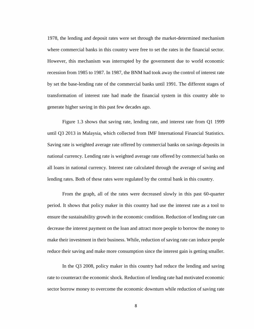
1978, the lending and deposit rates were set through the market-determined mechanism

where commercial banks in this country were free to set the rates in the financial sector.

However, this mechanism was interrupted by the government due to world economic

recession from 1985 to 1987. In 1987, the BNM had took away the control of interest rate

by set the base-lending rate of the commercial banks until 1991. The different stages of

transformation of interest rate had made the financial system in this country able to

generate higher saving in this past few decades ago.

Figure 1.3 shows that saving rate, lending rate, and interest rate from Q1 1999

until Q3 2013 in Malaysia, which collected from IMF International Financial Statistics.

Saving rate is weighted average rate offered by commercial banks on savings deposits in

national currency. Lending rate is weighted average rate offered by commercial banks on

all loans in national currency. Interest rate calculated through the average of saving and

lending rates. Both of these rates were regulated by the central bank in this country.

From the graph, all of the rates were decreased slowly in this past 60-quarter

period. It shows that policy maker in this country had use the interest rate as a tool to

ensure the sustainability growth in the economic condition. Reduction of lending rate can

decrease the interest payment on the loan and attract more people to borrow the money to

make their investment in their business. While, reduction of saving rate can induce people

reduce their saving and make more consumption since the interest gain is getting smaller.

In the Q3 2008, policy maker in this country had reduce the lending and saving

rate to counteract the economic shock. Reduction of lending rate had motivated economic

sector borrow money to overcome the economic downturn while reduction of saving rate

9

had induce people increased their consumption to maintain the same level of business

activity.

Figure 1.3: Saving, lending, and interest rates of Malaysia

Source: International Financial Statistics (IMF)

Figure 1.4 shows the classification of loans by purpose in Malaysia from 2006

until 2013. From the graph, most of the Malaysia’s borrowers make their loans for the

purpose of working capital, residential property and non-residential property, and

transportation. By comparing the amounts of total loan of RM 6,947,968.8 million in

2006 and RM 13, 996,631 million in 2013, the loan was highly increased by about

101.45% in this 8-year period.

Despite the loan for working capital, the loan for residential property had

remained the strongest one in this past eight years. Although the composition of

residential property to total loan remained 27-28% in these past 8 years, its total value

0

2

4

6

8

10

12

Q1

19

99

Q3

19

99

Q1

20

00

Q3

20

00

Q1

20

01

Q3

20

01

Q1

20

02

Q3

20

02

Q1

20

03

Q3

20

03

Q1

20

04

Q3

20

04

Q1

20

05

Q3

20

05

Q1

20

06

Q3

20

06

Q1

20

07

Q3

20

07

Q1

20

08

Q3

20

08

Q1

20

09

Q3

20

09

Q1

20

10

Q3

20

10

Q1

20

11

Q3

20

11

Q1

20

12

Q3

20

12

Q1

20

13

Q3

20

13

saving rate

lending rate

Interest rate (average of saving and lending rates)

10

showed incredible result. In 2006, the total loan for purchasing residential property was

only RM 1,876,950.54 million. However, the loan had sharply increased to RM

3,899,083.47 million after 8 years, which showed about 107.74% changes. It may

probably due to the households’ expectation on housing price in the future. The

expectation of higher housing price in the future had induced home buyers demand for

house nowadays and thus increased the loan for purchasing residential property in these

past eight years. Although home buyers can borrow money from the financial institution

to buy house, they still need to make the down payment by using their saving. This

economic phenomena has generating the motivation for undertaking this research to

examine the impact of housing price toward the saving behaviour in this country.