The Economic Effects of a Borrower Bailout:Evidence from an Emerging Market∗

Xavier Gine† Martin Kanz‡

Abstract

We study the credit market implications and real effects of one the largest borrowerbailout programs in history, enacted by the government of India against the backdropof the 2008–2009 financial crisis. We find that the stimulus program had no effect onproductivity, wages or consumption, but led to significant changes in credit allocationand an increase in defaults. Post-program loan performance declines faster in districtswith greater exposure to the program, an effect that is not driven by greater risk-takingof banks. Loan defaults become significantly more sensitive to the electoral cycle afterthe program, suggesting the anticipation of future credit market interventions as animportant channel through which moral hazard in loan repayment is intensified.

JEL: G21, G28, O16, O23Keywords: bailout, economic stimulus, crisis resolution, moral hazard

∗We thank the Reserve Bank of India and the various State Level Bankers Committees for sharing data used in this paper.We thank Sumit Agarwal, Bo Becker, Patrick Bolton, Emily Breza, Baghwan Chowdhry, Shawn Cole, Rob Garlick, RainerHaselmann, Asim Khwaja, Andres Liberman, Daniel Paravisini, Dina Pomeranz, Amit Seru, Rui Silva, James Vickery as wellas seminar participants at CEPR-ESSFM Gerzensee 2014, IGIDR Emerging Markets Finance 2014, FIRS 2014, Indian Schoolof Business, London Business School EWFC 2014, National University of Singapore, NEUDC (Harvard Kennedy School) andThe World Bank for helpful comments and suggestions. Maulik Chauhan and Avichal Mahajan provided outstanding researchassistance. Financial assistance from the World Bank Research Support Budget is gratefully acknowledged. The opinionsexpressed do not necessarily represent the views of the World Bank, its Executive Directors, or the countries they represent.† The World Bank, Development Research Group, 1818 H Street NW, Washington, DC 20433. Email: xgine@worldbank.org‡ The World Bank, Development Research Group, Email: mkanz@worldbank.org

1 Introduction

Since the Great Depression, economic stimulus programs have been ubiquitous during times

of economic crisis in advanced and developing economies. In their simplest form, such

programs provide direct subsidies or income support to households through the tax code.

In many cases, however, economic stimulus programs operate through the credit market,

typically in the form of debt restructuring and debt relief programs designed to encourage

investment and consumption during economic downturns.

Stimulus programs that operate through the credit market remain controversial among

economists and policymakers for at least two reasons. First, as in the case of fiscal stimulus

programs more generally, critics question whether ex-post credit market interventions can

affect real economic activity (Agarwal et al. [2005], Mian and Sufi [2012]) Second, while pro-

ponents argue that stimulus programs through the credit market may strengthen household

balance sheets and prevent excessive deadweight losses in times of economic crisis (Bolton

and Rosenthal [2002], Mian et al. [2013], Mian and Sufi [2014]), opponents argue that credit

market interventions are a particularly harmful way of implementing an economic stimulus,

as they change the contracting environment and may generate bank and borrower moral

hazard. Although credit market-led stimulus programs are common, there is surprisingly

little evidence on how they affect credit market outcomes and the real economy.

We address these questions by evaluating one of the largest borrower bailout programs

in history, enacted by the government of India against the backdrop of the global financial

crisis of 2008–2009. The program, known as the “Agricultural Debt Waiver and Debt Relief

Scheme” (Adwdrs), consisted of unconditional debt relief for more than 60 million rural

households across India, amounting to a volume of more than US$ 16 billion (approximately

1.7% of GDP). We exploit a natural experiment generating variation in bailout exposure to

estimate the effect of the bailout on the credit market and real economic activity.

1

The key challenge in identifying the causal effect of the bailout is the difficulty of con-

structing a valid counterfactual. Because cross-sectional exposure to the debt relief is a

function of loan delinquencies prior to the program, one might worry that estimates of pro-

gram impact are endogenous to pre-existing economic trends. To address this concern, our

identification strategy takes advantage of plausibly exogenous cross-sectional variation in

program exposure, generated by the Adwdrs program eligibility rules. We additionally

validate our credit market estimates using bank-district data, which allows us to exploit

within-district variation to explicitly control for local shocks to credit demand.

We find that the bailout had a significant and economically large effect on post program

credit allocation and loan performance. A one standard deviation increase in bailout ex-

posure led to a 4-6% decline in the number of loans and a 13-16% decline in the amount

of credit outstanding. The results also reveal a significant reallocation of credit away from

districts with high exposure to the bailout. While districts with high (above median) pro-

gram exposure received 36 cents of new lending for every 1 dollar of credit written off under

Adwdrs, districts with low (below median) program exposure received 4 dollars for every 1

dollar of debt relief. Despite this reallocation of new bank lending to observably “less risky”

districts, we document a significant decline in loan performance in districts with high bailout

exposure, concentrated among borrowers that had previously been in good standing.

In the second part of our analysis, we examine the effect of debt relief on the real economy.

Supporters of Adwdrs, including India’s government at the time, cited debt overhang and

investment constraints as one of the key motivations for the program and argued that debt

relief could not only provide immediate relief to households, but also improve agricultural

investment, with positive implications for rural productivity, wages and consumption. We

use detailed, regionally disaggregated data to test for the effect of the bailout on rural

productivity, wages and employment. Our results identify a precise zero for each of these

outcomes. This is consistent with household-level evidence on the impact of Adwdrs (see

2

Kanz [2012]), implies a low spending multiplier of debt relief, and suggests that the program

did not achieve the impact on real economic activity claimed by its proponents.

There are several reasons that make India’s bailout for rural households an especially

attractive setting to explore the impact of a credit market-led stimulus program. First, Ad-

wdrs is representative of a wide range of stimulus programs executed through interventions

into the credit market. In the United States, federal and state governments have frequently

intervened into debt contracts, with some of the largest credit market interventions occur-

ring in the aftermath of the Great Depression (Rucker and Alston [1987]). More recently,

in the context of the 2008 financial crisis, it has been argued that the weakness of house-

hold balance sheets, rather than the breakdown of financial intermediation, precipitated the

crisis and remains the main obstacle to economic recovery (see, for example, Mian and Sufi

[2011], Mian and Sufi [2014], Mian et al. [2014]). This “household balance sheet view” of the

crisis implies that debt relief for mortgage holders could have positive effects (Agarwal et al.

[2013], Guiso et al. [2013]). Stimulus programs enacted through the credit market have been

comparatively more frequent in developing economies, where debt relief and restructuring

programs have often targeted the economically and politically influential rural sector. Recent

examples include a US$ 2.9 billion bailout for farmers in Thailand and the restructuring of

more than US$ 10 billion of household debt in Brazil.

Second, India’s Adwdrs program was a one-off initiative that left the institutional en-

vironment unchanged, thus allowing us to isolate the effect of debt relief. Beneficiaries were

identified, settlements were made and lenders were recapitalized in a way that modified

existing loans but did not affect the rules and regulations governing new lending.

Third, unlike any previous debt relief initiative in India, eligibility for the program de-

pended on the amount of land pledged at the time of loan origination, typically many years

prior to the program. This rule, which applied retrospectively, provides a source of exogenous

variation in program exposure as it implies that the share of credit that could qualify for the

3

program is a function of the historically determined land distribution in a given district.

To the best of our knowledge, this paper provides the first empirical evidence on the

effects of large-scale debt relief on credit market outcomes and the real economy and thus

contributes to several strands of the finance literature. The “household balance sheet view” of

the financial crisis suggests that the strengthening of households’ balance sheet through debt

relief should have an unambiguously positive effect on the real economy.1 India’s Adwdrs

bailout followed this policy recommendation closely, by waiving household debts at a time

when credit markets were not in distress and before bad debts in the country’s important

rural sector could impair financial intermediaries. Hence, India’s Adwdrs offers an unusual

opportunity to assess the importance of the household balance sheet channel.

Most closely related to our paper, Agarwal et al. [2013] study the Home Affordability

Modification Program (Hamp), a subsidized mortgage restructuring program enacted in the

United States in the wake of the financial crisis. Although the scale of the program remained

relatively small, they find that the program led to a modest reduction in foreclosures but

had no effect on durable and non-durable consumption. Alston [1983], Alston [1984] and

Rucker and Alston [1987] study debt moratoria in the United States in the aftermath of the

Great Depression. Their results suggest that the short-term benefits of debt relief may have

come at the cost of moral hazard and credit rationing in the longer run.

Our results are also complementary to, but distinct from, a growing literature on the

effects of economic stimulus programs more broadly. Mian and Sufi [2012] study the impact

of the “Cash for Clunkers” stimulus program in the Unites States, which offered consumers

direct subsidies for new car purchases. They find that the stimulus shifted the timing of new

car purchases but did not affect employment, or default rates in cities with higher exposure to

the stimulus. Chodorow-Reich et al. [2014] study the American Recovery and Reinvestment1There are several reasons why this policy was not actively followed in the United States, including fears

of moral hazard and a possible reduction of future bank lending. See, for example, “Lawrence Summers onHouse of Debt” The Financial Times, June 6, 2014 for a discussion.

4

Act (Arra) and find positive employment effects of the program. These studies relate to the

literature on government spending and the Ricardian Equivalence (Barro [1989], Agarwal et

al. [2007], Nakamura and Steinsson [2014]). While our analysis differs from this literature

by focusing specifically on the impact of a credit market-led stimulus program, our results

suggest a low spending multiplier from debt relief.

Because the bailout affected not only borrowers but was also tied to a recapitalization

of banks by the Reserve Bank of India, our results are also related to the literature on bank

recapitalizations and the transmission of financial shocks to the real economy (Peek and

Rosengren [2000], Khwaja and Mian [2008], Paravisini [2008], Schnabl [2012], Lin and Par-

avisini [2013]), as well as more recent work on bank recapitalizations (Philippon and Schnabl

[2013] and Gianetti and Simonov [2013]). In line with this literature, we find evidence of im-

portant changes in bank lending and credit allocation. Reflecting a long history of directed

lending policies, Indian banks faced significant incentives to lend to sub-prime borrowers and

engage in “evergreening” of de facto non-performing loans (see Peek and Rosengren [2005]).2

The introduction of Adwdrs partly removed this incentive distortion, so that one would

expect the bailout to change both the level as well as the geographical allocation of post-

program lending. Consistent with this prediction, we find evidence of a shift in post-program

lending away from districts with high exposure to the bailout. Importantly, this also sug-

gests that the bailout did not encourage greater risk-taking by banks and thus enables us to

distinguish the effect of Adwdrs on bank risk-taking from its impact on borrower behavior.

Finally, we contribute to the literature on the political economy of credit in emerging

markets (Dinc [2005], Cole [2009b], Agarwal et al. [2012]). We find that loan performance

responds to the electoral cycle, and that this effect is magnified in the period after the bailout

is enacted. This finding underscores the concern that the anticipation of future credit market2See Banerjee et al. [2009] and Banerjee and Duflo [2014] for a discussion of the history and economic

impact of India’s directed lending policies. See Burgess and Pande [2005] and Burgess et al. [2005] for ananalysis of specific features of India’s directed lending policies.

5

interventions generated by the bailout is an important channel through which moral hazard

in loan repayment is intensified. It also suggests that the moral hazard costs of credit market

stimulus programs are likely to be particularly severe in economies with weak institutions

and a history of politically motivated credit market interventions.

The remainder of the paper proceeds as follows. In Section 2, we provide an overview of

India’s Adwdrs bailout program for rural households. Section 3 describes the data. Section

4 discusses the effect of the bailout on credit supply and loan performance, while Section 5

documents the real effects of the program. Section 6 presents additional robustness checks,

and 7 concludes.

2 India’s Bailout Program for Rural Households

India’s Adwdrs bailout for highly indebted rural households was announced in March 2008,

against the backdrop of the global financial crisis of 2007–2008.3 The goal of Adwdrs was

twofold. First, owing to a long history of directed lending to the rural sector, Indian banks

had accumulated significant amounts of non-performing loans. The bailout was intended to

strengthen Indian banks by eliminating substantial non-performing assets from their books

and recapitalizing the banks in the process. Second, the significant reduction of household

debt as a result of Adwdrs was intended to strengthen household balance sheets and act

as a direct stimulus for investment and consumption in India’s important rural sector.4

Introduced a year ahead of national elections, the program also represented a significant

transfer from urban to rural voters.

The rules for program eligibility were kept deliberately simple to expedite the processing

of claims, and to minimize opportunities for leakage and corruption at local bank branches3The Indian economy remained relatively unaffected by the global financial crisis, and credit spreads

indicate that Indian credit markets were not in distress at the time of the program announcement.4In 2008, agriculture accounted for approximately 15% of India’s GDP and 55% of total employment.

6

tasked with identifying eligible borrowers. In contrast to prior initiatives, individual eligibil-

ity depended on the amount of land pledged as collateral at the time a loan was originated,

typically several years before the program. Borrowers who had pledged less than two hectares

of land were eligible for full debt relief, while those that had pledged more than two hectares

of collateral qualified for 25% conditional debt relief if they repaid the remaining balance.

Loans that (i) had been originated between December 31, 1997 and December 31, 2007,

(ii) were 90+ days past due as of December 31, 2007 and (iii) remained in default until

February 28, 2008, qualified for the program. Importantly, the eligibility rules, including the

collateral cutoff, applied retrospectively, so that there was no scope for manipulation around

program dates. In addition, Adwdrs was the first debt relief program in India’s history to

use landholdings as a basis for eligibility and thus the rules were unanticipated.

Implementation of the program began in June 2008. Every bank branch in the country

was asked to identify all loans and borrowers on its books that met the bailout eligibility

criteria. As a transparency measure, branches were required to publicly post these beneficiary

lists, including the identity of the borrower, the details of the qualifying loan and collateral

pledged at the time of loan origination. Borrowers who qualified for debt relief had their

collateral cleared through a verifiable entry in their land documents, so that they were free

to use their collateral documents to access new loans. Banks were, in principle, required

to make Adwdrs beneficiaries eligible for new loans, although anecdotal evidence and our

results below suggest that many banks did not follow this directive.

Borrower lists underwent independent audits at the branch and bank level, and a formal

audit and redress mechanism was put in place by the regulator. Banks were recapitalized

by the central government through the Reserve Bank of India for the full amount of credit

written off under the program. Because eligibility rules were straightforward, reporting was

standardized, and implementation as well as audits were overseen by the same regulator,

enforcement of program was remarkably uniform, both geographically and across banks.

7

Unconditional debt relief, which accounted for approximately 81% of claims, was pro-

cessed immediately so that virtually all claims had been settled by the end of June 2008.

The deadline for settling claims under the partial debt relief scheme for loans with collateral

of more than two hectares of land was extended several times because of slow take-up –first

to December 2009, and subsequently to December 2010. To ensure that we accurately cap-

ture the total amount of debt relief granted in a district, our analysis relies on data collected

in December 2011, when the program was closed and all claims had been settled.

The Adwdrs program received significant media attention and was the center of an in-

tense political debate. Proponents of the program heralded the bailout as a cure for endemic

problems of debt overhang and poor investment incentives in the rural sector. Responses

to the program from the financial sector were more wary and warned, in particular, about

the potentially detrimental effects of the bailout for credit discipline and future access to

credit among borrowers benefiting from the bailout. The Economist, for example, noted

“Some fear that the government’s largesse will do lasting damage to a culture of prudent

borrowing, productive investment and prompt repayment.”5

3 Data and Descriptive Statistics

We examine the impact of India’s bailout for rural households using data at the district

and bank-district level. Our main dataset is a panel covering 489 (of 593 total) districts

of India from 2001 to 2012.6 Our primary unit of analysis is an Indian census district, an

administrative unit roughly comparable to a U.S. county. In the base year 2001, India had

593 districts with an average population of 1,731,897 inhabitants. In that year, the dis-5“Waiving, not drowning: India writes off farm loans. Has it also written off the rural credit culture?”

The Economist. June 3, 2008.6Between 2001 and 2012, 47 new districts were created, typically by bifurcating existing ones. In our

analysis, we aggregate all data to the level of India’s 2001 census districts.

8

tricts in our data set account for approximately 95% of the Indian population and 89% of

total bank credit.7 The dataset contains first, a measure of the intensity of cross-sectional

exposure to the Adwdrs bailout, measured as the share of agricultural credit eligible to

be written off in each district as a result of the Adwdrs program; second, detailed data

on credit market outcomes for each district, including the number of loans, lending volume

and loan performance; and third, credit market data merged with district-level information

on real economic outcomes, including agricultural productivity, rural wages and per capita

consumption. In this section, we describe each set of variables in turn.

3.1 Measuring Program Exposure

To measure a district’s exposure to the Adwdrs bailout, we collected data on the amount

of debt relief granted under the program from each state’s State Level Bankers’ Committee

(Slbc), the administrative body responsible for maintaining data on publicly supported

credit market programs within each state. We were able to obtain this information for 23

of India’s 28 states, including all major states of mainland India.8 For each district in the

data, we observe the amount of credit eligible for the bailout, consisting of overdue principal

and accumulated interest, and the amount of debt relief actually disbursed.

Using this dataset, we construct our measure of program exposure. Because settlement

was voluntary for borrowers above the two hectare collateral cutoff, our preferred measure of

program exposure uses the share of credit eligible to be forgiven under the Adwdrs program.

Letting crediti denote the total amount of outstanding agricultural credit in district i at the7Bank lending in India is typically concentrated within a district, and very little lending takes place

across district boundaries. This is the result of India’s long-standing branch banking regulations, underwhich branch licenses and lending targets are typically assigned at the sub-district or “block” level. Weexclude branches located in India’s largest metropolitan areas, Ahmedabad, Bangalore, Chennai, Jaipur,Hyderabad, Kolkata, Mumbai, and New Delhi, where the geographical mapping between bank and borrowerlocation is less likely to hold.

8Data were not available for the Northeastern states Arunachal Pradesh, Assam, Meghalaya, Nagalandand Mizoram. In the base year, these states account for less than 10% of total credit outstanding.

9

time of the program deadline (February 28, 2008), with superscript S denoting the share of

debt owed by households below the two hectare eligibility cutoff and superscript L denoting

debt owed by households above the cutoff, and letting si denote the share of credit that

was current at the time of the program deadline (and hence unaffected by the bailout), the

program exposure of district i can be written as

Bailout sharei =(1− si)

[creditS

i + .25κicreditLi

]creditS

i + creditLi

(3.1)

where κi denotes the fraction of loans settled under the partial debt relief option for house-

holds above the two hectare cutoff. Because settlement was optional for households above

the two hectare threshold, we assume κi = 1 for all i (full compliance among households

above the cutoff), which is equivalent to estimating the intent-to-treat effect for households

with more than two hectares of land pledged as collateral.

Table I reports summary statistics for the intensity of program exposure and highlights

significant variation in the share of credit forgiven as a result of the bailout. At the time

the program came into effect, the median district in our sample had approximately US$ 47

million of agricultural credit outstanding and saw approximately one third of this amount

written off as a result of the Adwdrs bailout (28.4%, s.d.=22.4).

Figure 1, Panel [b], plots the geographical distribution of program exposure and illustrates

the significant cross-sectional variation in program exposure, which is key to our identification

strategy. It is worth noting that bailout exposure does not appear to correlate significantly

with state boundaries or the distribution of credit prior to the program (see Figure 1, Panels

[a] and [b]). This suggests that program exposure is driven primarily by variation in economic

shocks ahead of the bailout, rather than longer-term differences in state-level institutions or

the development of local credit markets.

10

3.2 Lending and Loan Performance

Our credit market dataset combines district-level information on lending by all commer-

cial banks in India, provided by the regulator, with proprietary data on lending and loan

performance at the bank-district level, obtained from India’s largest commercial banks.

(a) District-level. Our main source of credit market data is the Reserve Bank of India’s

Basic Statistical Returns of Commercial Banks in India (BSR) dataset, which is an annual

panel of bank lending at the district level. The BSR data are based on annual “census” of

credit and cover the lending activities of all commercial banks in India at more than 100,000

bank branches across the country. Unless otherwise indicated, we focus on direct agricultural

credit, the type of credit that was most directly affected by the Adwdrs program, and use

data on Total credit (district) and Total loans (district) for the years 2001 to 2012. Summary

statistics for these variables, which are our primary measure of credit allocation, are reported

in Table II. In the base year 2001, the median district had a total of 22,744 agricultural loans

outstanding with a an average (median) loan size of US$ 515 (US$ 379).

(b) Bank-district level. We augment our credit market dataset with information on lend-

ing and loan performance at the bank-district level. Because data at this level of disaggrega-

tion is not made available by the regulator, we construct a new dataset based on proprietary

data from India’s four largest commercial banks. This data set contains information on

lending and loan performance for 1,783 bank-district pairs observed annually between 2006

to 2012. In the base year 2001, the data cover 27,678 bank branches, accounting for approx-

imately 40% of India’s network of bank branches and 62% of total credit. We again focus on

direct agricultural loans and construct the variables Total credit (bank-district) and Total

loans (bank-district).

Because data on loan performance at the sub-national level is not disclosed by the reg-

ulator, the bank-district panel is also our main source of information on loan performance.

11

We use the data set to construct the outcome variables Non-performing loans (number of

accounts) and Non-performing loans (share of credit). The data, summarized in Table II,

reveal significant cross-sectional and time series variation in loan performance. The median

bank branch in the sample records a non-performing loan share of 6% (s.d.20). In the pre-

program period, the median non-performing loan share stands at 13.6% (s.d.=12.3). This

figure gets reduced to 6.25% (s.d.=7.3) in the first year after the Adwdrs bailout.

3.3 Productivity, Wages, and Employment

Our primary source for data on agricultural productivity is the Indian Agricultural Statistics

database,9 which contains district-level information on crop yields and area planted for the

25 most common crops grown in India. We combine this data with commodity prices to

calculate the variable Productivity, which measures the value of agricultural production per

hectare in each district and year in the dataset. Because we wish to focus on the component

of productivity that can be affected by households, we use constant commodity prices for

the base year 2001, so that our measure of productivity may be interpreted as a measure of

quantity TFP (TFPQ).

The Indian Agricultural Statistics database also provides district-wise wages for unskilled

rural labor. Wages are reported seasonally, for every district in India and for a range of agri-

cultural occupations. We focus on unskilled daily wages for field and non-field agricultural

labor and calculate the variable Real wage, which measures a district’s rural wage as the av-

erage of these two wage groups over all crop seasons for which data are available, to account

for seasonal variation in labor demand and rural wages.

Data on household consumption are calculated from the Indian National Sample Survey9The dataset is published by the Indian Ministry of Agriculture and consists of the database of Agricultural

Wages in India (AWI), as well as the database on Agricultural Prices and Crop Yields (APY). Appendix Eprovides additional information on the construction of variables based on the dataset.

12

(NSS). The NSS is conducted annually as a repeated cross-sectional survey of approximately

75,000 rural and 45,000 urban households. We use data from four NSS survey rounds, two

prior to the bailout and two after the bailout,10 and calculate the variable Consumption,

which measures monthly per capita consumption expenditure (Mpce). This measure of

household consumption is collected consistently across survey rounds and widely used in

practice, for example in the calculation of poverty lines.11

3.4 Additional Variables

Our dataset contains a number of additional variables, which we use as controls and to con-

struct the instrumental variable described below. Specifically, we measure weather shocks

using local variation in monsoon rainfall. Rainfall data are taken from the Indian Meteoro-

logical Department and measure total monthly precipitation at the district level. Based on

these data, we construct the variable Rain monsoon, which measures total monsoon rainfall

between July and September for each year as a fraction of the district’s long-run rainfall

average over the same period.12 Based on this dataset, we also construct a dummy variable

indicating years in which a district was exposed to a drought shock. This variable takes on a

value of one for any year in which a district’s total monsoon rainfall between the months of

July and September was below 75% of the district’s long run precipitation average, measured

over the same time period. This definition matches the threshold used by Indian state and

local authorities to declare a district as “drought affected”.13

10We use data from NSS rounds 63 and 64 for the period prior to the bailout and NSS rounds 66 and 67for the period after the bailout.

11One possible limitation of using NSS data to estimate household consumption is that the NSS survey isrepresentative at the “survey unit,” rather than the district level (a survey unit typically consists of severalcensus districts). We therefore restrict the sample to districts with at least 50 NSS households.

12We use 50-year averages for June-September, taken from the Indian Meteorological Department’s dataset“Long Run Averages of Climatological Normals.”

13Data and definitions are available from the India Meteorological Department at http://www.imd.gov.in

13

Previous work has shown that lending of state banks in India tracks the electoral cycle.14

Hence, we control for a district’s temporal distance to the next scheduled state election to

account for the resulting fluctuations in credit supply. Electoral data come from the Election

Commission of India’s publicly available election statistics database. Finally, we use data on

district characteristics from the Census of India and the Indian Agriculture Census. These

data include the population and land distribution of each district.

4 The Credit Market Effects of the Bailout

Estimating the credit market impact of the bailout poses two main identification challenges.

First, program exposure is a function of loan defaults ahead of the program, and therefore

potentially endogenous to pre-existing economic trends at the district level. Second, esti-

mating the causal effect of the program requires us to distinguish changes in credit supply

from contemporaneous shocks to credit demand.

We address this identification problem in two steps. First, we estimate the credit market

impact of the bailout at the district level, using a difference-in-differences specification, in

which we instrument for program exposure. Since we observe both program exposure and

real outcomes at the district level, we use this approach as our benchmark identification

strategy. Second, we verify the robustness of our credit market estimates by replicating the

analysis with data at the bank-district level. This allows us to isolate the impact of the

bailout on credit supply from any contemporaneous shocks to credit demand using a fixed

effects strategy similar to Khwaja and Mian [2008].15 As we shall see, both identification

strategies yield similar point estimates.14Cole [2009b] shows that agricultural lending by state-owned banks in India increases by 5-10 percentage

points in election years.15This approach been used in a number of studies that identify the transmission of credit shocks through

the bank lending channel. See, for example, Schnabl [2012], Paravisini et al. [2014] and others.

14

We begin by estimating the impact of the bailout on credit market outcomes, using

difference-in-differences specifications of the form

ln(Cit) = αi + βt · dr + γEit +X ′itζ + εit (4.1)

where Cit is a credit market outcome for district i (in region r) and year t, the variable

Eit (Bailout sharei × Postt) measures a district’s exposure to the bailout program, αi are

district fixed effects and βt are time fixed effects, which we allow to vary across the four

administrative regions dr, i ∈ r of the Indian central bank to account for heterogeneity in

local business cycles. Xit is a vector of observable determinants of credit market conditions,

which always includes lagged monsoon rainfall and a full set of electoral cycle dummies.16 The

coefficient of interest γ measures the effect of program exposure on credit market outcomes,

and the error term εit captures all omitted factors, including any deviations from linearity.

We drop all observations for 2008, the year in which the program took effect, to rule out any

mechanical correlation between treatment intensity and observed credit market outcomes,

and estimate equation 4.1 using data for 489 districts observed between 2001 and 2012, for

a total of 5,511 observations.

Equation 4.1 will consistently estimate γ if Cov(Eit, εit)=0. This covariance restriction

may, however, not hold if exposure to the program is correlated with unobserved trends

in credit market outcomes. To address this concern, we rely on an instrumental variables

strategy based on the rule that a loan had to be both in default and backed by land collateral

of less than two hectares to qualify for unconditional debt relief. This eligibility rule allows

us to use two sources of exogenous variation to instrument for program exposure. The first

source of variation is the time series of weather shocks17 experienced by a district prior to16See Cole [2009b] for evidence that lending by Indian state banks co-moves with the electoral cycle for

local (state assembly) elections.17We use years in which total monsoon rain between June and September was below 75% of the district’s

long-run average rainfall as our definition of weather shocks. This definition is consistent with the threshold

15

the program, which is a strong predictor of loan defaults. The second source of variation is

a district’s land distribution, which determines the fraction of households that fall below the

two hectare cutoff and could have been eligible for unconditional debt relief.

We thus use the number of drought years, wit, experienced by a district in the period

prior to the bailout, interacted with the share of households below the eligibility cutoff, `i,

to obtain a cross-sectional predictor of the share of credit bailed out in each district:18

Zi =t∑

t=1wit · `i (4.2)

We then interact this variable with an indicator that marks the beginning of the program,

to construct a time-varying instrument for program exposure:

Zit = t∑

t=1wit · `i

× Postt (4.3)

It is important to stress that even if one of these two plausibly exogenous sources of variation

were to affect outcomes through a channel other than program exposure, the interaction be-

tween weather shocks and the collateral cutoff should become relevant only as a result of the

program. We verify this empirically and provide additional identification tests in Appendix

B. In particular, we first check that there is no correlation between the instrument and any

of our credit market outcomes prior to the program. Second, we show that the instrument is

also uncorrelated with observable district characteristics in the year the program came into

effect. Our instrumental variables strategy yields the first-stage specification

Eit = δi + θt · dr + γfsZit +X ′itζfs + εit (4.4)

used by Indian state and local authorities to declare a district as “drought affected.”18The present day land distribution of India’s districts is largely the result of land reforms enacted under

British colonial rule (see Banerjee and Iyer [2005] for a detailed discussion) and therefore plausibly exogenousto economic trends over the comparatively short time period we study.

16

where, as in equation 4.1 above Eit is the program exposure of district i at time t in region r,

Xit is a matrix of observable determinants of credit market conditions and we control for year

and district fixed effects. Table III presents estimates of the first stage and demonstrates

that the instrument is a relevant predictor of program exposure. The first stage coefficient

γfs is positive and statistically significant at the 1% level (γfs=0.257, s.e.=0.049), indicating

that districts with greater exposure to pre-program drought shocks and a greater share of

households below the eligibility cutoff saw a significantly higher share of credit waived as

a result of the program. An F -Statistic of 23.16 for the regression corresponding to our

preferred specification (Table III, column [4]) implies a strong first stage.

One potential concern with our identification strategy is that that the treatment effect

estimated in equation 4.1 confounds the impact of the bailout on credit supply with possible

contemporaneous shocks to credit demand. To rule out this possibility, we use an alternative

identification strategy based on Khwaja and Mian [2008]. In particular, we derive an esti-

mating equation at the bank-district level from a simple model of credit supply and demand.

This approach has several advantages. First, taking the identification from the district to

the bank-district level allows us to isolate the effect of the bailout from shocks to credit

demand by controlling for district-time fixed effects. Second, we can identify the aggregate

bank lending channel separately from the effect that the bailout has on the within bank

reallocation of credit across districts with differential program exposure.19 The derivation,

described in Appendix C, yields the following estimating equation

ln(Cijt) = ξit + γEEjt + γBBijt + χijt (4.5)19The model underlying our estimating equation makes several testable predictions. First, banks experi-

encing a larger equity shock as a result of greater overall exposure to the bailout should increase lending(γE>0). At the same time, banks should redistribute lending away from districts with greater programexposure, as the program allows them to clean troubled assets from their books and thus reduces incentivesthat may have existed to “evergreen” loans close to default prior to the program (γB<0). This can be testedagainst the alternative hypothesis that the program encouraged banks to engage in riskier lending. If thiswere the case, then one would expect γE>0 and γB>0.

17

where ξit are district-time fixed effects, Ejt denotes the equity shock received by bank j as

a result of the bailout and Bijt denotes program exposure (the share of total credit written

off under the program) at all branches of bank j in district i.

As we show in more detail below, the estimates from the two alternative identification

strategies are quantitatively similar, although standard errors are expectedly narrower when

we use bank-district level data.

4.1 Impact on Credit Allocation

In this subsection, we use the methodology described above to estimate the effect of the

bailout on credit market outcomes. We begin by estimating the impact of the bailout on

credit allocation and present evidence to corroborate the hypothesis that the patterns we

observe are driven by changes in the supply of credit that occur in response to the bailout.

Table IV reports the results, using the specification in equation 4.1. The dependent

variable in columns [1] to [4] is the log number of loans, while in columns [5] to [8] the

dependent variable is the log amount of credit. For each dependent variable, the first two

columns report OLS estimates while the second set of columns present two-stage least squares

(2SLS) results using the instrumental variable strategy described in the previous section.

Within each set of estimates, the first column controls for district fixed effects as well as

time varying controls. The second column presents results from a more flexible specification

that allows each district to follow its own linear time trend in the pre-program period.

We find that that bank lending becomes more conservative as a result of the bailout.

While overall lending increases after the program, the results indicate that banks reallo-

cate credit away from districts with greater program exposure. The magnitude of credit

reallocation in response to the bailout is economically large. Estimates from our preferred

specification in Table IV, columns [4] and [8] indicate that a one standard deviation increase

18

in the share of credit covered by the program leads to a 3.6% decrease in new loans made

after the bailout (γ=-0.036, s.e.=0.068). The shift of bank lending away from high bailout

districts is both larger and more precisely estimated when the amount of credit is used as the

dependent variable. Our results indicate that a one standard deviation increase in program

exposure leads to a 15% decrease in new lending after the program (γ=-0.150, s.e.=0.068).

We also estimate a modified version of our baseline specification that uses the total

amount of credit as the outcome of interest and replaces our measure of program exposure

by the total amount of credit eligible for the program in a given district. In this specification,

the difference-in-differences estimate γ can be interpreted as the amount of new lending per

dollar of bailout exposure. The results, reported in Appendix A, suggest an asymmetric

reallocation of credit away from high bailout districts as a result of Adwdrs. While districts

with high (above median) program exposure receive only 36 cents of new lending for every

1 dollar of credit written off under the program, districts with low (below median) bailout

exposure receive an average of 4 dollars of new lending for every 1 dollar of debt relief.

The finding that banks channel new lending to observably less risky districts after the

bailout may seem counterintuitive, given that the empirical literature on bank recapitaliza-

tions has generally found a positive correlation between bailouts and bank risk-taking. The

pattern of reallocation we find is, however, consistent with the hypothesis that the bailout

affected incentives for “evergreening” (Peek and Rosengren [2005]), that is, to keep lending

to borrowers close to default in an attempt to avoid marking these loans as non-performing.

Reflecting a long history of directed lending (see Burgess and Pande [2005], and Banerjee and

Duflo [2014]), all banks in India are required to allocate 40% of their net credit to “priority

sectors”, which include agriculture and small scale industry. While this mandate forces the

allocation of a significant share of credit to sub-prime borrowers, local branch managers also

face strong penalties for realizing credit losses. This creates a significant incentive to keep

lending to borrowers close to default. The introduction of Adwdrs removed this incentive

19

distortion. Consistent with the “evergreening” hypothesis, we find evidence of a shift in

post-program bank lending away from districts with greater bailout exposure.

Table VI implements the specification in equation 4.5, which uses bank-district level data

and controls for district-time fixed effects to verify that the results from our preferred speci-

fication are not driven by changes in credit demand. As in Table IV, column [1] uses the log

number of accounts as the dependent variable, and column [2] uses log credit as the outcome

of interest. To allow for a meaningful comparison, we restrict the sample in Table VI to

the districts included in our estimation of equation 4.1. We find that banks experiencing

a larger equity shock as a result of their bailout increase their overall lending, but reallo-

cate credit away from districts with greater exposure to the bailout. The point estimates

are negative and significant for both the number of loans (γB=-0.210, s.e.=0.033) and the

amount of credit (γB=-0.142, s.e.=0.045), and the size of these effect is even larger than

in the district-level estimates reported in Table IV. Taken together, these results indicate a

strong supply-side response that is not confounded by changes in credit demand.

4.2 Impact on Loan Performance and Moral Hazard

We next examine the effect of the bailout on ex-post loan performance. Table V presents

the results, using the basic specification described in equation 4.1. The dependent variable

columns [1] to [4] is a dummy equal to one if the branches in a given district experienced an

increase in the share of non-performing loans between year t− 1 and t, while the dependent

variable in columns [5] to [8] is a dummy equal to one if bank branches located in a given

district experienced an increase in the share of non-performing credit over the same time

period. As before, our preferred specification includes a full set of fixed effects, time-varying

controls and linear pre-trends for each district (columns [4] and [8]).

We find evidence of a strong negative effect of the bailout on loan performance. The

20

coefficient estimate from our preferred specification indicates that a one standard deviation

increase in bailout exposure leads to a 69% increase in the probability that a district ex-

periences the share of non-performing loans (γ=0.691, s.e.=0.385), and a 64% increase in

the probability that a district experiences an increase in the share of non-performing credit

(γ=0.642, s.e.=0.355) in the post-program period.

Table VI, columns [3] and [4] verifies that the results on loan performance also hold at the

bank-district level using the fixed effects specification described in equation 4.5. The results

are again consistent with those found in our preferred specification. Banks that received

a greater share of bailout funds are significantly more likely to experience an increase in

defaults after the program, and districts in which bank branches were more exposed to the

bailout experience a decline in loan performance after the program. It is important to note

that this decline in loan performance happens after loans that were in default have been

written off and cleared from banks’ books. Given that Table IV columns [1] to [4] show

no evidence of new lending, we conclude that the negative effect of the bailout on loan

performance is driven by defaults among borrowers that were previously in good standing.

Table VI, columns [5] and [6] estimate the size of this effect using bank-district level data and

suggest that it is substantial. The point estimates indicate a one standard deviation increase

in bailout exposure is associated with a 1.6% increase in the share of non-performing loans

(γB=0.016, s.e.=0.003) and a 2.4% increase in the share of non-performing credit (γB=0.024,

s.e.=0.003) over the sample mean.

Taken together, these results point to substantial borrower moral hazard. First, loan

performance after the program deteriorates in districts with greater bailout exposure even

though banks reallocate credit towards observably less risky districts. Second, because no

new lending took place and non-performing loans covered by the program were removed

from banks’ books, post-program defaults must be concentrated among borrowers that were

previously in good standing (and therefore not covered by the bailout). The program thus

21

created perverse incentives among non Adwdrs beneficiaries to default strategically.

One possible concern with this interpretation is that higher default rates in high-bailout

districts might be explained by other changes in credit conditions, such as a change in

average loan sizes that would have impacted the repayment capacity. In unreported results,

we find no evidence of a systematic change in average loan sizes as a result of the bailout.

Furthermore, Appendix B presents an additional that exploits the exogenous timing of Indian

state elections. We show that electoral cycles in loan defaults are magnified in the post-

program period. On average, defaults in pre-election years increase by approximately 5

percentage points over the post-program sample mean of 7.25% (γ=0.131, s.e.=0.076). In

addition, average loan sizes do not vary around elections prior to the bailout or after the

bailout. This indicates that the anticipation of future credit market interventions generated

by the bailout is a key channel through which moral hazard in loan repayment is intensified.

Another interpretation, perhaps less plausible, is that the tightening of credit in high-

bailout districts led to a slowdown of economic activity thus causing the increase in defaults

among non Adwdrs beneficiaries. The next section studies the real effects of the bailout

and finds little support for this interpretation.

5 Real Effects of the Bailout

The principal aim of economic stimulus programs is to stabilize output, and to prevent dis-

tortions in investment and consumption during economic downturns. In the case of India’s

Adwdrs bailout, proponents of the program argued that debt relief could stimulate pro-

ductive investment by alleviating problems of endemic debt overhang in India’s important

agricultural sector. Given the scale of the bailout, it was thought that the program might

not only restore access to institutional credit for rural households, but also provide a direct

stimulus to household consumption and the rural labor market.

22

In this section, we evaluate this hypothesis by exploring the impact of the Adwdrs

program on real outcomes. We are interested in estimating the elasticity of non-financial

outcomes with respect to program exposure (the share of credit forgiven as a result of the

program). To do so, we use district-level data on agricultural productivity, real wages and

household consumption and estimate equations of the form

ln(Rit) = αi + βt · dr + ωZit +X ′itζ + νit (5.1)

where Rit is a real outcome of interest for district i observed at time t, αi are district fixed

effects, and βt are time fixed effects, which we again allow to vary across India’s four central

bank regions dr, i ∈ r to account for local variation in business cycles. The variable Zit

measures the instrumented district’s exposure to the bailout, and Xit is a vector of time

varying controls. In this equation, the coefficient of interest ω measures the elasticity of real

outcomes with respect to program exposure. We estimate this equation using data at the

district level, the most granular level at which information on real outcomes is available.

Hence, we cannot use district-year fixed effects to separately identify exposure to the bailout

from time-varying demand shocks, as in equation 4.5 above. As in equation 4.4 before,

bailout exposure is instrumented using the interaction between the number of drought years

prior to the bailout and the share of households below the Adwdrs collateral threshold.

We first explore the effect of debt relief on agricultural productivity. We focus on agri-

cultural productivity as the outcome that we would expect to be most directly affected if the

bailout alleviated problems of debt overhang, as claimed by its proponents. Indeed, house-

hold indebtedness is high in India’s large agricultural sector, and producers rely heavily on

external financing, usually provided by commercial banks, to undertake productive invest-

ments. Proponents of the Adwdrs bailout generally argued that the debt relief initiative

would create incentives for productive investment and free collateral so that rural house-

23

holds could access new credit. If the program had this effect, we would expect this to be

reflected in greater investment and increased agricultural productivity. To test whether this

is the case, we take advantage of a district level panel on crop yields and commodity prices

from the Indian Department of Agriculture. The dataset, which we describe in Section 3

and Appendix E, contains detailed information on agricultural revenue and area cultivated,

which allows us to construct time series of agricultural productivity over the time period

2001-2011 for 387 districts in our sample. Table VII, columns [1] to [4], estimate the impact

of the stimulus program on agricultural productivity. The results show that the program

had no discernible effect on agricultural productivity. Using our preferred specification, the

estimated effect is a precise zero (γ=-0.006, s.e.=0.010), suggesting that the stimulus did

not create investment incentives of a magnitude sufficient to affect agricultural productivity.

Second, we investigate the effect of debt relief on real wages, to test for a possible la-

bor market impact of the bailout. Unskilled labor is an important input to agricultural

production. Hence, if the bailout had a positive impact on households’ ability to invest in

productive inputs, one might expect to find this effect reflected in rural employment. To

test for this channel, we construct a panel of real wages for the period 2006-2011. The data

capture monthly wages for unskilled agricultural labor in a sample of 327 districts, which

we average for all agricultural occupations and over all reported crop seasons to account for

seasonal fluctuations in labor demand. In columns [5] to [8], we test for an impact of the

bailout on rural wages using the same regression specifications as in columns [1] to [4], and

do not find a discernible effect of the bailout using. The coefficient estimate from our pre-

ferred specification is negative, close to zero (γ=-0.07, s.e.=0.099) across all specifications.

The result also remains unchanged when we restrict the sample to non-urban districts with

a rural population share of 75 percent and above.

Finally, we turn to the effect of the bailout on household consumption. If households

perceived the bailout as a permanent change in their access to credit and more productive

24

inputs, they may have increased consumption. To test for an effect on household consump-

tion, we construct a panel of mean per capita expenditure (Mpce), the standard measure of

household consumption, using NSS micro-data as described in Section A.I and Appendix E.

We estimate the impact of debt relief on consumption in Table VII, columns [9] to [12], and

again find that the bailout had no measurable positive effect on household consumption.

The government believed that a recapitalization of banks would encourage new lending

and that this, in turn, would stimulate new investment through the removal of disincentives

for investment and the strengthening of households balance sheets. These positive effects,

however, were not realized as lenders reallocated credit away from bailout districts driven,

in part by the anticipation of borrower moral hazard as a result of the program.

6 Robustness Tests

In this section, we present additional identification and robustness tests in two steps: we

first report several tests of the difference-in-differences identification assumption, requiring

that outcomes follow parallel trends before the program. Second, we check that our results

are not confounded by a differential response to weather shocks in districts with different

land distributions (e.g. a greater share of large landholdings).

The difference-in-differences strategy underlying our empirical approach relies on the

assumption that outcomes for the treatment and control groups –in our case districts with

different levels of bailout exposure– do not follow differential trends in the pre-program

period and would have followed identical trends in the absence of the intervention. We now

present three tests of this assumption.

We begin by presenting graphical tests of the parallel trends assumption for our main out-

comes of interest. Figure 2 and Figure 3, plot lending and loan performance for high-bailout

(above median) and low-bailout (below median) districts. The graphs show no indication

25

that the parallel trends assumption is violated for our main credit market outcomes. Figure

4 shows parallel trends plots for real outcomes, again differentiating between districts above

and below the median program exposure. There is again no indication that the parallel

trends assumption is violated for these outcomes.

However, given that our treatment variable (the share of credit forgiven in each district)

is continuous, one may be concerned that these simple graphical tests may mask deviations

from the parallel trends assumption among a subset of districts. We address this possibility

by presenting additional parametric tests of the parallel trends assumption.

In the first set of parametric tests of the parallel trends assumption, we estimate regres-

sions in which we allow each district to follow its own linear time trend in the pre-program

period. These estimates are reported as the second specification for each group of regressions

in Tables IV to VII. The results indicate that the inclusion of linear time trends improves

the precision of the point estimates, but does not qualitatively affect our main findings.

In the second set of parametric tests, we explore the possibility that our estimates are

affected by the presence of non-linear trends. To do so, we perform two placebo experiments.

In the first placebo experiment, we restrict our sample to the pre-bailout period and move the

timing of the bailout from 2008 to a hypothetical program date in 2005. The results, reported

in Table VIII, columns [1] to [5], show that the treatment coefficients for the hypothetical

program date are close to zero and, in several cases have the opposite sign, indicating that

the treatment effect at the actual program date is not driven by unobserved time trends.

The second placebo experiment tests for the presence of non-linear time trends by ran-

domly reassigning treatment levels among the cross-section of districts in our sample. We

do this using a bootstrap procedure, in which we draw N=1,000 random assignments of

our treatment vector, estimate treatment coefficients using our preferred specification, and

report bootstrap coefficients and standard errors obtained from this exercise. The estimated

treatment effects, reported in Table VIII, columns [6] to [10], are again close to zero and

26

statistically insignificant. In sum, these results make it unlikely that our results are biased

as a result of deviations from the parallel trends assumption.

Finally, we explore the possibility that our results are driven by differential responses to

weather shocks at the district level. In Section 4 and Appendix B, we test the plausibility

of the exclusion restriction for our instrumental variables estimates. In particular, we show

that there is no correlation between the interaction of drought shocks and a district’s land

distribution before the bailout. In this section, we test for the possibility that the bailout

shock had a differential post-program impact in districts with a different land distribution.

If this were the case, our estimates of the post-program path of credit market variables and

real effects would be biased by underlying differences in district characteristics, and provide

an inaccurate estimate of the credit shock. We test this possibility by estimating a version

of equation 4.1 in which we control for the share of landholdings in district i that are larger

than four hectares, interacted with the variable post, which takes on a value of one for all

years after 2008. This effectively restricts identification of the program impact to a band of

{Cutoff−2ha, Cutoff +2ha}, thus controlling for the possibility that shock responses differ

in “landlord districts” with a significant share of large landholdings. Table IX presents the

results. With the exception of the extensive margin of credit, for which the effect is weaker

and less precisely estimated, we do not find any significant changes relative to our baseline

estimates. This makes it unlikely that our results are driven by differential shock responses

arising from underlying differences in a district’s land distribution.

7 Conclusion

The world over, governments have routinely intervened in credit markets in an effort to

stimulate economic activity. While credit market led stimulus programs are extremely com-

mon, they are often thought to have negative implications for credit allocation and borrower

27

discipline, without generating a sufficiently large offsetting effects on real economic activity.

There exists however surprisingly little evidence to evaluate these claims. This paper uses

a natural experiment arising from one of the largest borrower bailouts in history –India’s

Adwdrs debt relief program for highly indebted rural households– to estimate the causal

effect of a large credit market stimulus and makes two main contributions.

First, we show that the bailout led to a significant reallocation of bank lending away

from districts with greater exposure to the bailout. A one standard deviation increase in

the share of credit waived under the program leads to a 13-16% decline in new bank lending

in the district after the program. This reallocation of new credit towards observably better

performing districts is prima facie evidence that the bailout removed incentives to “evergreen”

(Peek and Rosengren [2005]), thus allowing for a more efficient allocation of credit.

Second, we find that the program had no positive impact on productivity, consumption

or labor market outcomes, but led to significant moral hazard in loan repayment. These

results indicate that the program had a significant moral hazard cost that is not offset by

a positive impact on productivity, consumption or the rural labor market. Importantly, we

show that the increase in defaults is concentrated among borrowers that were previously in

good standing, and is not driven by greater bank risk-taking or a change in the debt levels

of existing borrowers. Moreover, the relationship between defaults and the electoral cycle

–which exists in normal times and has been documented in earlier studies– is magnified

by the bailout, suggesting that the anticipation of future credit market interventions is an

important channel through which moral hazard in loan repayment is intensified.

The results also shed light on the importance of the household balance sheet channel

in crisis resolution. In the case of the United States it has been argued that high levels of

accumulated household debt –rather than the breakdown of financial intermediation– were

an important factor precipitating the financial crisis of 2008 (see Mian and Sufi [2011],Mian

and Sufi [2014], and Mian et al. [2014]). This view would suggest that a program similar

28

to that implemented in India under the Adwdrs bailout should have an unambiguously

positive effect on the real economy. In contrast, we find no evidence of greater investment,

consumption or positive labor market outcomes in areas where debt relief led to a significant

reduction of household debt. It is not surprising that, in the case of India, government efforts

to stimulate the real economy through debt relief were largely in vain given that the bailout

also led lenders to reallocate credit away from districts with high program exposure.

While our results do not dispute the potentially important role of the household balance

sheet channel, they highlight the difficulty of designing debt relief programs in a way that

ensures the transmission of the credit market stimulus to the real economy. In particular, our

findings underscore the importance of taking into account the impact of debt relief on post-

program credit supply. The reallocation effect we find is likely exacerbated by two features

of the program. First, Adwdrs covered primarily term loans with short maturity, which

were fully written off and eliminated from banks’ balance sheets as soon as the program

came into effect. Hence, Indian banks were free to immediately reallocate credit away from

regions with high bailout exposure. This contrasts with the partial write down of longer-term

mortgage debt proposed in the United States, which would have presumably not terminated

lending relationships entirely. Second, the Adwdrs bailout made debt relief mandatory and

treated willful defaulters and genuinely distressed borrowers alike. This is likely to give rise

to significant ex-post moral hazard among borrowers who could have repaid but were bailed

out and borrowers who did not qualify for debt relief because they had remained current

on their loan payments throughout. The results suggest that this moral hazard cost of debt

relief is fueled by the expectation of future government interference in the terms of existing

credit contracts, and is thus likely to be especially severe in weak institutional environments

with a history of politically motivated credit market interventions.

29

ReferencesAgarwal, Sumit, Chunlin Liu, and Nicholas Souleles, “The Reaction of Consumer

Spending and Debt to Tax Rebates: Evidence from Consumer Credit Card Data,” Journalof Political Economy, 2007, 115 (4), 986–1019.

, G. Amromin, I. Ben David, and Serdar Dinc, “The Legislative Process and Fore-closures,” Working Paper, 2012.

, G., I. Ben David, S. Chomsisengphet, T. Piskorski, and A. Seru, “PolicyIntervention in Debt Renegotiation: Evidence from the Home Affordability ModificationProgram,” Working Paper, 2013.

, S.Chomsisenghpet, and O. Hassler, “The Impact of the 2001 Financial Crisis andthe Economic Policy Response on the Argentine Mortgage Market,” Journal of HousingEconomics, 2005, 14 (3), 242–270.

Alston, Lee, “Farm Foreclosures in the United States During the Interwar Period,” Journalof Economic History, 1983, 43 (4), 885–903.

, “Farm Foreclosure Moratorium Legislation: A Lesson From the Past,” American Eco-nomic Review, 1984, 74 (2), 445–457.

Banerjee, Abhijit and Esther Duflo, “Do Firms Want to Borrow More? Evidence froma Directed Lending Program,” Review of Economic Studies, 2014, 81 (1).

and Lakshmi Iyer, “History, Institutions, and Economic Performance: The Legacyof Colonial Land Tenure Systems in India,” American Economic Review, 2005, 95 (4),1190–1213.

, Shawn Cole, and Esther Duflo, “Default and Punishment: Incentives and LendingBehavior in Indian Banks,” Harvard Business School Working Paper, 2009.

Barro, Robert J., “The Ricardian Approach to Budget Deficits,” Journal of EconomicPerspectives, 1989, 3 (2), 37–54.

Bolton, Patrick and H. Rosenthal, “Political Intervention in Debt Contracts,” Journalof Political Economy, 2002, 110 (5), 1103–1134.

Burgess, Robin and Rohini Pande, “Do Rural Banks Matter? Evidence from the IndianSocial Banking Experiment,” The American Economic Review, 2005, 95 (3), 780–795.

, Grace Wong, and Rohini Pande, “Banking for the Poor: Evidence From India,”Journal of the European Economic Association, 2005, 3 (2/3), 268–278.

30

Chodorow-Reich, Gabriel, Laura Feiveson, Zachary Liscow, and William Wool-ston, “Does State Fiscal Relief During Recessions Increase Employment? Evidence fromthe American Recovery and Reinvestment Act,” American Economic Journal: EconomicPolicy, 2014, 4 (3), 118–145.

Cole, Shawn A., “Financial Development, Bank Ownership, and Growth. Or, Does Quan-tity Imply Quality?,” The Review of Economics and Statistics, 2009, 91 (1), 33–51.

, “Fixing Market Failures or Fixing Elections? Elections, Banks and Agricultural Lendingin India,” American Economic Journal: Applied Economics, 2009, 1 (1), 219–250.

Dinc, Serdar, “Politicians and Banks: Political Influences on Government-Owned Banksin Emerging Markets,” Journal of Financial Economics, 2005, 77 (1), 453–479.

Gianetti, Mariassunta and Andrei Simonov, “On the Real Effects of Bank Bailouts:Micro Evidence from Japan,” American Economic Journal: Macroeconomics, 2013, 5 (1),135–167.

Guiso, Luigi, Paola Sapienza, and Luigi Zingales, “The Determinants of Attitudestoward Strategic Default on Mortgages,” Journal of Finance, 2013, 68 (4), 1473 – 1515.

Kanz, Martin, “What Does Debt Relief do for Development? Evidence from India’s Bailoutfor Highly-Indebted Rural Households,” World Bank Policy Research Working Paper 6258,2012.

Khwaja, Asim and Atif Mian, “Tracing the Impact of Bank Liquidity Shocks: Evidencefrom an Emerging Market,” American Economic Review, 2008, 98 (1), 1413–1442.

Lin, Huidan and Daniel Paravisini, “The Effect of Financiang Constraints on Risk,”Review of Finance, 2013, 17 (1), 229–259.

Mian, Atif, Amir Sufi, and Francesco Trebbi, “Foreclosures, House Prices and theReal Economy,” Forthcoming, Journal of Finance, 2014.

and , “House Prices, Home Equity -Based Borrowing, and the U.S. Household LeverageCrisis,” American Economic Review, 2011, 100 (5), 2132–2156.

and , “The Effects of Fiscal Stimulus: Evidence from the 2009 Cash for ClunkersProgram,” Quarterly Journal of Economics, 2012, 127 (3), 1107–1142.

and , “What Explains the 2007-2008 Drop in Employment?,” Forthcoming, Economet-rica, 2014.

, Kamalesh Rao, and Amir Sufi, “Household Balance Sheets, Consumption and theEconomic Slump,” Quarterly Journal of Economics, 2013, 128 (4), 1687–1726.

31

Nakamura, Emi and Jon Steinsson, “Fiscal Stimulus in a Monetary Union: Evidencefrom U.S. Regions,” American Economic Review, 2014, 104 (3), 753–792.

Paravisini, Daniel, “Local Bank Financial Constraints and Access to External Finance,”Journal of Finance, 2008, 63 (5).

, Veronica Rappoport, Philipp Schnabl, and Daniel Wolfenzon, “Dissecting theEffect of Credit Supply on Trade: Evidence from Matched Credit-Export Data,” WorkingPaper, 2014.

Peek, Joseph and Eric Rosengren, “Collateral Damage: Effects of the Japanese BankCrisis on Real Activity in the United States,” American Economic Review, 2000, 90 (1),30–45.

and Eric S. Rosengren, “Unnatural Selection: Perverse Incentives and the Misalloca-tion of Credit in Japan,” American Economic Review, September 2005, 95 (4), 1144–1166.

Philippon, Thomas and P. Schnabl, “Efficient Recapitalization,” Journal of Finance,2013, 68 (1), pp. 1–42.

Rucker, Randal and L. Alston, “Farm Failures and Government Intervention: A CaseStudy of the 1930s,” The American Economic Review, 1987, 77, 724–730.

Schnabl, Philipp, “The International Transmission of Bank Liquidity Shocks: Evidencefrom an Emerging Market,” Journal of Finance, 2012, 67 (3), 897–932.

32

Data Sources

Table A.I Description of Variables

Variable Description SourcesDrought years The number of “drought years” experienced by a district prior to the

program. A drought year is defined as a year in which total monsoonrainfall between June and September was below 75 percent of a district’s50-year average. The variable counts the number of drought years in thepre-program period between the years 2001 and 2007. Rainfall data comesfrom the Indian Meteorological Department (IMD), Long-run normals aretaken from India Meteorological Department Long Run Averages ofClimatological Normals, CD-ROM.

India MeteorologicalDepartment (IMD)

Electoral cycle Five dummy variables indicating the temporal distance to the nextscheduled state assembly election. State assembly elections are scheduledevery five years and are staggered over time.

Election Commissionof India, available athttp://eci.nic.in.

Householdconsumption

Mean per capita household expenditure (MPCE), calculated fromhousehold-level data of the Indian National Sample Survey.

India National SampleSurvey (various years)

Land distribution Share of landholdings in the district that are smaller than two hectares(approximately 5 acres) in size.

India AgricultureCensus, DistrictTables (2001)

Non-performing loans,amount

This information is not publicly available. We have calculated it fromproprietary data obtained from India’s four largest commercial banks. (a)At the bank-district level, the data consist of annual information on theamount of outstanding rural credit and the amount of rural NPAs (bothdenominated in units of Rs 100,000) and cover the years 2006-2012. (b) Atthe district level, our measure of loan performance is the arithmetic mean ofloan performance for all banks with branches in the district. To ensureconsistency with the credit data, we exclude districts for which we have noinformation on program exposure.

Proprietary bank data.

Non-performing loans,number of loans

This information is not publicly available. We have calculated it fromproprietary data obtained from India’s four largest commercial banks. (a)At the bank-district level, the data cover the years 2006-2012 and consist ofannual information on the number of outstanding agricultural loans and thenumber of loans in default, defined as 90+ days past due (b) At the districtlevel, our measure of loan performance is the arithmetic mean of loanperformance for all banks with branches in the district. To ensureconsistency with the credit data, we exclude districts for which we have noinformation on program exposure.

Proprietary bank data.

Rainfall Total monsoon rainfall as a share of the 50 year district-level average.Monsoon rainfall is defined as total rainfall between June and September.Long-run normals are taken from India Meteorological Department LongRun Averages of Climatological Normals, CD-ROM.

India MeteorologicalDepartment (IMD)

Rural wage Real unskilled wage for all agricultural occupations, measured at the end ofthe main crop season each year. Data are available for the years 2001-2011.

Indian Ministry ofAgriculture

Total agriculturalproductivity

Revenue per hectare derived from the sale of 32 main crops. Data onagricultural yields is available from the Indian Ministry of Agriculture,revenues are calculated using constant 2001 commodity prices. Data areavailable for the years 2001-2011.

Indian Ministry ofAgriculture, Indiastat

33

Table A.I: Description of Variables (cont’d)Variable Description SourcesTotal credit, amount The natural logarithm of outstanding agricultural credit in units of Rs

100,000 for each district of India. (a) The district-level data are constructedfrom the Reserve Bank of India’s BSR dataset, and cover all agriculturalloans made by private, public, cooperative and regional rural banks for theyears 2001-2012. (b) The bank-district level data are taken from proprietarydata on agricultural lending at all branches of India’s four largestcommercial banks and covers the years 2006-2012.

Reserve Bank of India,Basic StatisticalReturns of ScheduledCommercial Banks inIndia, (2001 -2012);proprietary bank data.

Total credit, numberof loans

Total number of agricultural loans outstanding. (a) District-level data areconstructed from the Reserve Bank of India’s Basic Statistical Returns ofcommercial Banks in India (BSR) dataset, and include all agricultural loansmade by private, public, cooperative and regional rural banks. We use datafor the years 2001-2012 (b) At the bank-district level, this variable isconstructed from proprietary data on agricultural lending at all branches ofIndia’s four largest commercial banks. The dataset covers the period2006-2012 and contains district level aggregates of approximately 27,678branches in all states and Union Territories of India (Reserve Bank of India,A Profile of Banks, 2012).

Reserve Bank of India,Basic StatisticalReturns of ScheduledCommercial Banks inIndia, (2001 -2012);proprietary bank data.

34

Tables and Figures

Table IProgram Exposure

This table reports summary statistics for the variable Bailout share,our main measure of program exposure. The variable measures thetotal amount of credit eligible for the bailout as a share of totaloutstanding agricultural credit on March 31, 2008, the date whenthe bailout program was enacted. To facilitate the interpretationof our estimates, the variable is normalized to have mean zero andstandard deviation one in all subsequent tables.

Bailout share(N =489)

Mean .326Median .284StDev .224Min .002Max .991

35

Table IISummary Statistics

This table presents summary statistics for the datasets used in the analysis. Panel A summarizes the district-level dataset, containing information for 489 districts and the years 2001 to 2012. Total credit is the logamount of total agricultural lending (in Rs million). Total loans is the log number of total agricultural loansoutstanding. Loan performance at the district level is aggregated from the bank-district dataset describedin Panel B. Population is the log of a district’s total population. Rural share is the share of a districtspopulation living in rural areas. Productivity per hectare is the total revenue from all crops produced in adistrict at 2001 prices, divided by the total area planted. Rural wage is the log of the average daily wage foragricultural labor. Per capita consumption is the log of monthly per capita household consumption. Landholdings below 2 ha measures the share of total recorded landholdings in a district that are smaller than twohectares. Monsoon rain is the average precipitation recorded in a district between June and September as ashare of the district’s 50-year rain average over the same period. Drought years is the number of years between2001 and the 2007, in which a district experienced a drought, defined as a year in which monsoon rainfallwas less than 75 percent its long-run average. Time to election measures the number of years remaining untilthe next scheduled state election. Panel B summarizes the bank-district level dataset. All variables in thisdataset are based on proprietary data from India’s four largest banks, available for a panel of 569 districtsfor the years 2005 to 2012. Total credit is the log of total agricultural lending at these banks, and Total loansis the log number of agricultural loans. All monetary values are in nominal Indian Rupees. Table A.I andAppendix E provide additional details on data sources and the definition of variables.

(1) (2) (3) (4) (5) (6)Obs Mean Median StdDev Min Max

Panel A: District-level dataI. Lending and loan performanceTotal credit 6,952 9.20 9.46 1.80 1.75 14.52Total loans 6,952 10.10 10.36 1.52 2.08 14.71Non-performing loans, share of ag credit 6,574 0.14 0.06 0.20 0.00 1.00Non-performing loans, share of accounts 6,437 0.18 0.10 0.22 0.00 1.00II. District characteristicsTotal population 7,553 14.00 14.21 1.02 10.35 16.08Rural share 7,553 0.78 0.82 0.17 0.00 1.00III. Real outcomesProductivity per hectare 5,840 0.17 0.14 0.10 0.00 0.74Rural wage 1,031 4.36 4.32 0.43 3.29 5.75Per capita consumption 2,478 11.96 11.85 0.53 10.59 13.43IV. Additional controlsLand holdings below 2ha 6,669 0.53 0.56 0.24 0.00 .99Monsoon rain, % of 50-year mean 6,094 97.05 88.46 50.71 8.36 1062Drought years 7,008 0.87 0.00 1.48 0 7Time to election 7,540 2.01 2.00 1.41 0 4Panel B: Bank-district level dataI. Lending and loan performanceTotal credit 15,003 6.44 6.88 2.80 -4.61 12.75Total loans 10,170 6.13 6.48 2.74 0.00 12.56Non-performing loans, share of ag credit 14,987 0.11 0.04 0.17 0.00 1.00Non-performing loans, share of ag accts 10,763 0.15 0.08 0.20 0.00 1.00

36

Table IIIFirst Stage – Weather Shocks and Program Exposure

The regressions in this table estimate the first stage relationship between weather shocks andprogram exposure. The coefficient of interest measures how the interaction between the numberof drought years experienced by a district in the period between 2001 and 2007 and the shareof households below the two hectare eligibility cutoff affects program exposure. The dependentvariable in all regressions is the share of credit eligible for the program. We define a “drought year”as any year in which total precipitation during the monsoon months of June to September was lessthan 75 percent of a district’s long-run average. All regressions control for lagged monsoon rain,and a set of dummy variables indicating the number of years until the next schduled state election.Estimates in columns [2] to [4] add interactions between time and region fixed effects to control forheterogeneity in business cycles across regions and between urban and rural areas. Standard errors,in brackets, are calculated using the Huber-White correction for arbitrary heteroskedasticity andclustered at the district level. * p<0.10 ** p<0.05 *** p<0.01.

(1) (2) (3) (4)Dependent variable Program exposure

Drought years*Below cutoff 0.237*** 0.237*** 0.247*** 0.257***[0.046] [0.046] [0.047] [0.049]

Observations 4096 4096 4096 4096R-squared 0.061 0.061 0.101 0.774Joint F -Statistic 5.21 7.63 9.41 23.16Region*Year FE No Yes Yes YesDistrict FE No No Yes YesDistrict trends No No No YesClustered SE district district district district

37

Table IVCredit Supply – Effect on Post-Program Lending (District)

The regressions in this table estimate the impact of debt relief on post-program credit supply. For each dependent variable,each column reports results from a separate regression. The first two columns (columns [1]-[2] and [5]-[6]) report OLS estimates,the second two columns (columns [3]-[4] and [7]-[8]) report instrumental variables regressions using the first stage relationshipreported in Table III. The dependent variable in columns [1]-[4] is the log number of loans outstanding. The dependent variablein columns [5]-[8] is the log amount of credit outstanding. In addition to the fixed effects reported in the table, all regressionscontrol for the deviation of lagged monsoon rainfall from its long run average, a full set of electoral cycle dummies indicatingthe number of years until the next scheduled state election. Standard errors, in brackets, are heteroskedasticity robust andclustered at the district level. * p<0.10 ** p<0.05 *** p<0.01.

(1) (2) (3) (4) (5) (6) (7) (8)Dependent variable Log(Loans) Log(Amount)

OLS OLS 2SLS 2SLS OLS OLS 2SLS 2SLS

Bailout share*post -0.022 -0.058** -0.019 -0.036 -0.035*** -0.138*** -0.176*** -0.150**[0.014] [0.028] [0.037] [0.063] [0.013] [0.023] [0.045] [0.068]

observations 4,553 4,553 4,096 4,096 4,553 4,553 4,096 4,096# clusters 489 489 433 433 489 489 433 433R-squared 0.735 0.805 0.735 0.798 0.93 0.951 0.92 0.950Region*Year FE Yes Yes Yes Yes Yes Yes Yes YesDistrict FE Yes Yes Yes Yes Yes Yes Yes YesDistrict trends No Yes No Yes No Yes No YesClustered SE district district district district district district district district

38

Table VMoral Hazard – Effect on Post-Program Loan Performance (District)

The regressions in this table estimate the effect of debt relief on loan performance. For each dependent variable, each columnreports results from a separate regression. The first two columns (columns [1]-[2] and [5]-[6]) report OLS estimates, the secondtwo columns (columns [3]-[4] and [7]-[8]) report instrumental variables regressions, using the first stage relationship reportedin Table III. The dependent variable in columns [1]-[4] is a dummy variable equal to one if a district experienced an increasein the share of non-performing loans. The dependent variable in columns [5]-[8] is a dummy variable equal to one if a districtexperienced an increase in the share of non-performing credit. In addition to the fixed effects indicated in the table, all regressionscontain the full set of controls described in Table IV. Standard errors, reported in brackets, are heteroskedasticity robust andclustered at the district level. * p<0.10 ** p<0.05 *** p<0.01.

(1) (2) (3) (4) (5) (6) (7) (8)Dependent variable Non-performing loans (number of loans) Non-performing loans (share of credit)

OLS OLS 2SLS 2SLS OLS OLS 2SLS 2SLS

Bailout share*post 0.070*** 0.039 0.513** 0.691* 0.094*** 0.028 0.464** 0.642*[0.024] [0.062] [0.219] [0.385] [0.023] [0.060] [0.203] [0.355]

observations 2,246 2,246 2,023 2,023 2,278 2,278 2,055 2,055# clusters 460 460 412 412 460 460 412 412R-squared 0.091 0.303 0.081 0.231 0.172 0.42 0.036 0.358Region*Year FE Yes Yes Yes Yes Yes Yes Yes YesDistrict FE Yes Yes Yes Yes Yes Yes Yes YesDistrict trends No Yes No Yes No Yes No YesClustered SE district district district district district district district district

39

Table VIEffects on Credit Supply and Loan Performance (Bank-District)

The regressions in this table estimate the impact of debt relief on credit supply and loan performance,using panel data at the bank-district level. The dataset is based on proprietary data from India’sfour largest commercial banks and covers agricultural lending and loan performance at 27,678 bankbranches between 2006 and 2012. To allow comparability, the sample is restricted to the districtscontained in the district level dataset used in Tables IV and V. The first two columns examinethe effect of the bailout on credit supply. The dependent variable in column [1] is the log num-ber of agricultural loans outstanding. The dependent variable in column [2] is the log amount ofagricultural credit outstanding. The second two columns explore the effect of the bailout on loanperformance. The dependent variable in column [3] is the share of non-performing agricultural loans.The dependent variable in column [4] is the share of non-performing agricultural credit. The variableBailout shareij is a district’s exposure to the bailout program. Bailout sharej measures the meanbailout exposure of each bank across all districts in which it is present. To account for time-varyingcredit demand shocks, all regressions control for district-time fixed effects. Standard errors, in brack-ets, are calculated using the Huber-White correction for arbitrary heteroskedasticity and clusteredat the district-year level. * p<0.10 ** p<0.05 *** p<0.01.

(1) (2) (3) (4)Dependent variable Lending Loan performance

Log(Loans) Log(Amount) NPL(Loans) NPL(Amount)

Bailout shareij*post -0.193*** -0.240*** 0.018*** 0.027***[0.048] [0.036] [0.004] [0.003]

Bailout sharej*post 1.805*** 0.661*** 0.014*** 0.005***[0.077] [0.025] [0.004] [0.001]

observations 6,205 9,750 6,206 9,741# districts 489 489 489 489# clusters 2,918 3,006 2,918 3,006R-squared 0.612 0.427 0.556 0.393District*Year FE Yes Yes Yes YesClustered SE district-year district-year district-year district-year

40

Table VIIReal Effects of the Bailout – Productivity, Wages and Employment

The regressions in this table estimate the effect of debt relief on real outcomes, using a district-level data for the years 2006 to 2012. For eachdependent variable, each column reports results from a separate regression. The first two columns (columns [1]-[2], [5]-[6]) and [9]-[10] report OLSestimates, the second two columns (columns [3]-[4], [7]-[8] and [11]-[12]) report instrumental variables estimates based on the first stage regressionsin Table III. The dependent variable in columns [1]-[4] is district level productivity, calculated as agricultural revenue per hectare at constant 2001commodity prices. The dependent variable in columns [5]-[8] is the district level real wage for unskilled agricultural occupations. The dependentvariabe in columns [9]-[12] is the district level average of monthly per capita consumption expenditure (Mpce), calculated from Indian NationalSample Survey (NSS) microdata. Details on data sources and the construction of these variables are available in Table A.I and Appendix E. Inaddition to the fixed effects reported in the table, all regressions control for the deviation of lagged monsoon rainfall from its long run average,electoral cycle dummies indicating the number of years until the next scheduled state election. All regressions additionally control for time*regionfixed effects to account for business and credit cycle heterogeneity across regions. Standard errors, in brackets, are calculated using the Huber-Whitecorrection for arbitrary heteroskedasticity and clustered at the district level. * p<0.10 ** p<0.05 *** p<0.01.

(1) (2) (3) (4) (5) (6) (7) (8) (9) (10) (11) (12)Dependent variable Log(Productivity) Log(Real wage) Log(Consumption)

OLS OLS 2SLS 2SLS OLS OLS 2SLS 2SLS OLS OLS 2SLS 2SLS

Bailout share*post 0.001 0.000 -0.006 0.006 0.020 0.023 -0.018 -0.070 0.000 0.011 -0.053 -0.256**[0.002] [0.002] [0.010] [0.010] [0.016] [0.017] [0.074] [0.099] [0.008] [0.008] [0.075] [0.104]

observations 1,621 1,621 1,530 1,530 751 751 685 685 1,928 1,928 1,727 1,727R-squared 0.116 0.264 0.104 0.259 0.114 0.152 0.119 0.129 0.916 0.927 0.911 0.846Region*Year FE Yes Yes Yes Yes Yes Yes Yes Yes Yes Yes Yes YesDistrict FE Yes Yes Yes Yes Yes Yes Yes Yes Yes Yes Yes YesDistrict trends No Yes No Yes No Yes No Yes No Yes No YesClustered SE district district district district district district district district district district district district

41

Table VIIIRobustness – Placebo Experiments

This table reports the results of two placebo experiments testing for the presence of non-linear time trends in outcomes of interest. The firstplacebo experiment, reported in columns [1]-[4], restricts the sample to the period prior to the program date and estimates treatment effects fora counterfactual program date. The second placebo experiment, reported in columns [5]-[8], tests for the presence of unobserved non-linear timetrends. We generate N=1,000 vectors containing randomly reassigned values of the treatment variable and use these placebo treatment vectorsto estimate counterfactual program effects and bootstrap standard errors. Treatment effect estimates are obtained from regressions using thesame set of controls listed in tables IV and VI. * p<0.10 ** p<0.05 *** p<0.01.

(1) (2) (3) (4) (5) (6) (7) (8)Placebo [post=1(t≥2007)] Placebo [reassigned treatment]

Dependent variable Log(Loans) Log(Amount) NPL(Loans) NPL(Amount) Log(Loans) Log(Amount) NPL(Loans) NPL(Amount)

Panel A: Treatment effect estimatesBailout share*post -0.036 -0.150** 0.691* 0.464** -0.036 -0.150** 0.691* 0.464**

[0.063] [0.068] [0.385] [0.203] [0.063] [0.068] [0.385] [0.203]Panel B: Placebo estimatesBailout sharePlacebo*post -0.007 0.025 -0.109* -0.023 -0.010 -0.026 0.029 0.01095% Confidence interval [-0.125 [-0.113 [-0.223 [-0.136 [-0.079 [-0.138 [-0.001 [-0.008

0.111] 0.163] 0.005] 0.090] 0.059] 0.086] 0.056] 0.028]Region*Year FE Yes Yes Yes Yes Yes Yes Yes YesDistrict FE Yes Yes Yes Yes Yes Yes Yes YesDistrict trends Yes Yes Yes Yes Yes Yes Yes YesClustered SE district district district district district district district district

42

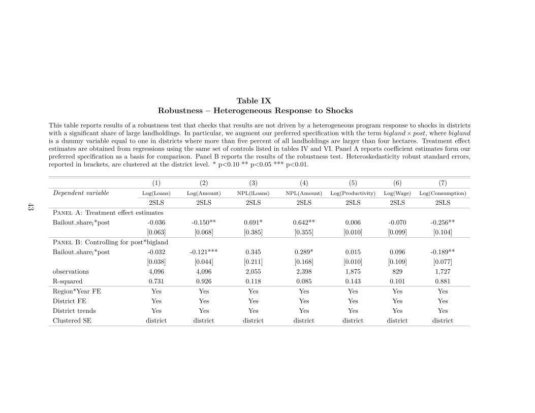
Table IXRobustness – Heterogeneous Response to Shocks

This table reports results of a robustness test that checks that results are not driven by a heterogeneous program response to shocks in districtswith a significant share of large landholdings. In particular, we augment our preferred specification with the term bigland× post, where biglandis a dummy variable equal to one in districts where more than five percent of all landholdings are larger than four hectares. Treatment effectestimates are obtained from regressions using the same set of controls listed in tables IV and VI. Panel A reports coefficient estimates form ourpreferred specification as a basis for comparison. Panel B reports the results of the robustness test. Heteroskedasticity robust standard errors,reported in brackets, are clustered at the district level. * p<0.10 ** p<0.05 *** p<0.01.

(1) (2) (3) (4) (5) (6) (7)Dependent variable Log(Loans) Log(Amount) NPL(lLoans) NPL(Amount) Log(Productivity) Log(Wage) Log(Consumption)

2SLS 2SLS 2SLS 2SLS 2SLS 2SLS 2SLSPanel A: Treatment effect estimatesBailout sharei*post -0.036 -0.150** 0.691* 0.642** 0.006 -0.070 -0.256**

[0.063] [0.068] [0.385] [0.355] [0.010] [0.099] [0.104]Panel B: Controlling for post*biglandBailout sharei*post -0.032 -0.121*** 0.345 0.289* 0.015 0.096 -0.189**

[0.038] [0.044] [0.211] [0.168] [0.010] [0.109] [0.077]observations 4,096 4,096 2,055 2,398 1,875 829 1,727R-squared 0.731 0.926 0.118 0.085 0.143 0.101 0.881Region*Year FE Yes Yes Yes Yes Yes Yes YesDistrict FE Yes Yes Yes Yes Yes Yes YesDistrict trends Yes Yes Yes Yes Yes Yes YesClustered SE district district district district district district district

43

Figure 1: Program Exposure by District

!

!

!

!!

!

!

!

!!

!

!

!

!!

!!

!!

!

!

!

!

!!

!

!

!

q1

q2

q3

q4

No data

(a) Credit per capita, pre-program!

!

!

!!

!

!

!

!!

!

!

!

!!

!!

!!

!

!

!

!

!!

!

!

!

q1

q2

q3

q4

No data

(b) Program exposure, share of credit forgiven

Notes: The figure plots the geographical distribution of agricultural credit per capita on March 31, 2008 (the date of the program announcement)in Panel (a) against district level exposure to the bailout, measured as the share of credit outstanding eligible for debt relief under the program inPanel (b). Both variables are plotted as quartiles, darker colors indicate higher amounts of credit per capita and bailout exposure, respectively.

44

Figure 2: Parallel Trends – Credit Supply

(a) Number of Loans [2001=100]

(b) Total Credit [2001=100]

Notes: The figure plots the time series of the number of agricultural loans outstanding in panel (a) andthe amount of agricultural credit outstanding in panel (b) for districts with “high” and “low” programexposure. Districts are classified into “high” and “low” program exposure relative to the median ofthe treatment variable. The shaded region marks the year in which the bailout program was enacted,which is omitted from the analysis.

45

Figure 3: Parallel Trends – Loan Performance

(a) Non-performing loans [accounts]

(b) Non-performing loans [share of credit]

Notes: The figure shows the time series of loan performance, measured as the share of non-performingagricultural loans in panel (a) and the share of non-performing agricultural credit in panel (b) fordistricts with “high” and “low” program exposure, respectively. Districts are classified into “high” and“low” program exposure relative to the median of the treatment variable. The shaded region marksthe year in which the bailout program was enacted, which is omitted from the analysis.

46

Figure 4: Parallel Trends – Real Effects

(a) Rural wages [2006=100]

(b) Productivity [2001=100]

Notes: The figure plots the time series of rural unskilled wages (a) and agricultural productivity,measured as revenue per hectare at constant 2001 commodity prices (b) for districts with “high” and“low” program exposure. Districts are classified into “high” and “low” exposure relative to the medianof the treatment variable. The shaded region marks the year in which the bailout program was enacted,which is omitted from the analysis.

47

Supplemental Appendix‘The Economic Effects of a Borrower Bailout: Evidence from

an Emerging Market’

Xavier Gine† Martin Kanz‡

A Post-Program Credit Supply: How much Reallocation?

In this appendix, we report an alternative measure of the credit reallocation from “high-bailout” to “low-bailout” districts in response to the bailout. To do this, we estimate adifference-in-differences model similar equation 4.1, but replace our measure of treatmentintensity by the total amount of credit eligible for the bailout in a given district. We thenestimate the effect of this variable on the net amount of post-program credit for districtsabove and below the median program expenditure, so that our coefficient estimates canbe interpreted as the amount of new lending per dollar of bailout received. The estimatesin Table A.I indicate that 1 dollar of bailout is associated with 2.4 - 4.1 dollars of newlending in low-bailout districts, but only 0.23 - 0.34 cents of new lending in high-bailoutdistricts. This provides evidence that banks actively reallocated credit away from districtswith poorer loan performance in the pre-program period. The results also suggest that thiscredit reallocation was asymmetric, with high-bailout districts suffering a disproportionatedecline in new lending after the program.

Table A.I Effect of the Bailout on Credit Supply – Reallocation

(1) (2) (3) (4)Amount credit

High-bailout district Low-bailout districtEligible amount*post 0.232* 0.336 2.437*** 4.078***

[0.136] [0.212] [0.268] [0.439]observations 2,276 2,276 2.277 2,277R-squared 0.736 0.844 0.787 0.870District FE Yes Yes Yes YesDistrict trends No Yes No YesClustered SE district district district district

† The World Bank, Development Research Group, 1818 H Street NW, Washington, DC 20433. Email: xgine@worldbank.org‡ The World Bank, Development Research Group, Email: mkanz@worldbank.org

48

B Pre-program Outcomes and District Characteristics

In this appendix, we present additional tests to validate our instrumental variables identifi-cation strategy.

First, one might be concerned the exclusion restriction is violated. The exclusion re-striction requires that the instrument –the interaction between the program cutoff and thenumber of pre-program drought years in a given district– affect outcomes only through itseffect on program exposure. This condition may be violated if, for example, changes in eco-nomic outcomes are significantly different in districts that are more prone to drought shocksor have a larger share of households below the two hectare collateral threshold.

While this cannot be tested directly, we address this possibility by estimating the con-ditional correlation between the instrument and outcomes of interest in the pre-programperiod. To perform this test, we restrict the sample to the period prior to the bailout and es-timate panel regressions estimating the correlation between the instrument (lagged for eachtime period) and pre-program outcomes. The results, reported in Table B.II, indicate thatthere is no correlation between the first stage and any of the main outcomes of interest inthe period prior to the bailout.

Table B.II Test – Effects on Pre-program Outcomes

(1) (2)Coefficient p-value

Dependent variable Drought years*cutoff (H0: No conditional correlation)Log(# loans) -0.012 [0.036] 0.739Log(amt credit) 0.002 [0.038] 0.957Non-performing loans -0.069*[0.040] 0.086Log(productivity) -0.002 [0.004] 0.610Log(rural wage) 0.018 [0.102] 0.860Log(consumption) -0.088 [0.086] 0.310

The second potential challenge to our identification strategy is the possibility that cross-sectional variation in the instrument correlates with district characteristics at the time ofthe bailout, in a way that puts districts on a different growth path in the post-programperiod for reasons unrelated to the program. We address this possibility by testing for adirect relationship between our first stage and a set of observable district characteristics atthe time of the program announcement. The results are presented in Table B.III. We findno evidence that our predictor of program exposure is systematically related to observabledistrict characteristics, such as the share of a district’s rural population or productivity thatmay have put districts on a different growth path in the post-program period for reasonsother than bailout exposure.

49

Table B.III Test – Effects on District Characteristics in 2008

(1) (2)Coefficient p-value

Dependent variable Drought years*cutoff (H0: No conditional correlation)Log(Population) -0.129 [0.132] 0.329Share rural population 0.006 [0.017] 0.713Log(Total ag credit) -0.064 [0.134] 0.633Log(Productivity) -0.012 [0.011] 0.282

C Derivation of Bank-District Level Regression Equation

This appendix presents a simple model of the credit market, from which we derive theestimating equation for credit market outcomes at the bank-district level. We model thebailout as an equity shock to the bank and relax the assumption that banks must lend in thesame district, as intended by the government. This allows us to derive an estimating equationin which we can separate the impact of the equity shock on the bank lending channel fromthe reallocation of post-program lending across districts where the bank has a presence.

Consider an economy in which j ∈ 1...J banks provide credit to borrowers in i ∈ 1...Ndistricts, so that the lending of bank j in district i at time t can be written as Cijt. Weassume banks can raise deposits at the marginal cost θDDijt, and that loans are financed byeither deposits or equity, so that each bank’s lending must be consistent with the identity

Cjt ≡ Djt + Ejt. (C.1)

In each period, banks may experience supply shocks ejt = et + ejt that determine thelevel of equity available to each bank. For the average district, the effect of this supply shockcan be written as Eijt = (et + ejt)/N , where N denotes the number of districts.

On the demand side, we assume that in any given period, a district may experience ademand shock δit = δt + δit with an economy-wide and a district-specific component. Hence,the marginal return of a loan Lijt is given by δt + δit − θCCijt − θBBijt, where Bijt is theamount of non-performing assets of bank j in district i. We assume that θC and θB ∈ [0, 1),so that the marginal return of an additional unit of credit to district i is declining in theamount of credit outstanding as well as the district’s stock of non-performing loans.

Equating marginal cost and marginal return, we obtain the condition θDDijt = δt + δit−θCCijt− θBBijt. Combining this expression with the identity in equation (C.1), we can solvefor the credit market equilibrium

Cijt =δt + 1

NθDet

θD + θL

+1NθD

θD + θL

ejt −θB

θD + θL

Bijt + 1θD + θL

δit (C.2)

The first term in this equation is an economy-wide time-varying constant that includes

50

demand and supply shocks. The last term is a district-specific time-varying constant. Bothcan be combined into a time-varying district fixed effect ξit. The second and third termscontain the main coefficients of interest. We can then rewrite equation (C.2) as follows

ln(Cijt) = ξit + γEejt + γBBijt + χijt (C.3)

This equation can be estimated directly, using credit data at the bank-district level, andallows us to isolate the impact of the bailout on credit supply by controlling for demandshocks using a simple fixed effects strategy. The model underlying our estimating equationpredicts that γE > 0 and γB < 0. That is, banks experiencing a larger equity shock (greaterbailout exposure) should increase lending. At the same time, banks should redistributelending away from districts with greater program exposure, as the program allows them toclean troubled assets from their books and thus reduces incentives that may have existed to“evergreen” loans close to default prior to the program (Peek and Rosengren [2005]). Thiscan be tested against the alternative hypothesis that the program encouraged banks to lendin a given district an amount proportional to the bailout funds received. If this were thecase, then one would expect γE > 0 and γB > 0.

D Mechanisms: Moral Hazard

The results in section 4.2 document that the Adwdrs bailout had a strong negative effecton loan performance, which does not appear to be driven by greater bank risk-taking. Inthis section, we present additional results to shed light on the mechanism behind this result.Specifically, we exploit the exogenous timing of Indian state elections to isolate changesin loan performance that occur for economic reasons from defaults that correlate with theelectoral cycle and can be regarded as pure moral hazard.

Our is based on the following argument. There are two potential channels that canlead to a decline in loan performance ahead of election years. First, electoral cycles indefault can arise from changes in credit market conditions, such as increased credit supply,reduced screening and monitoring standards and a change in loan sizes around elections.21

Second, electoral cycles in default can arise from moral hazard among borrowers who expectcredit enforcement to be more lenient in election years. If the bailout indeed induced moralhazard by heightening expectations of future credit market interventions, we would expectthe magnitude of political cycles in default to increase after the bailout, even when wecondition on credit market conditions and the local business cycle.

To test for this channel explicitly, we exploit the exogenous timing of Indian state elec-tions. Each of India’s 28 states holds state assembly elections on a 5-year cycle. Theseelections are staggered in time, with an average of 4–6 states holding elections in a given

21See Cole [2009b] and Cole [2009a]for evidence on politically motivated lending in India and politicalcycles in agricultural lending.

51

calendar year. We use this exogenous source of variation in Table D.IV, where we regressthe share of non-performing loans on an interaction between a post-program dummy andan indicator equal to one in the two years preceding a state election. Because state govern-ments have the power to call early elections, we define this variable with reference to thetime remaining to the next scheduled state election.

We find that electoral cycles in loan defaults are magnified in the post-program period.On average, defaults in pre-election years increase by an additional 1–2 percentage points(over the post-program sample mean of 7.25%) after the bailout. In unreported results, weverify that the greater loan delinquencies around election times are not driven by concurrentchanges in loan sizes that might affect the average debt burden and repayment capacity ofborrowers. We find no evidence of a systematic change in average loan sizes around electionsprior to the bailout or as a result of Adwdrs.

These results are consistent with the concern that the cost of politically motivated creditmarket interventions arises, to a significant extent, from their effect on borrower expectations.While our data do not allow us to test this hypothesis explicitly, one might expect thisadverse effect of credit market-led stimulus programs on borrower behavior to be particularlypronounced in credit markets with significant state ownership of banks and a history ofpolitically motivated credit market interventions, such as the one we study.

Table D.IV Mechanism – Defaults and the Electoral Cycle

(1) (2) (3) (4)Dependent variable NPL (Loans) NPL (Amount)

OLS OLS OLS OLS

Close to election*post 0.064* 0.081 0.132*** 0.131*[0.039] [0.073] [0.048] [0.076]

observations 3,096 3,096 3,096 3,096R-squared 0.270 0.461 0.27 0.462Region*Year FE Yes Yes Yes YesDistrict FE Yes Yes Yes YesDistrict trends No Yes No YesClustered SE district district district district

E Measuring Real Economic Activity

This section describes the construction of outcome variables used to analyze the effect of thebailout on real economic activity in Table VII.

Productivity: To construct a measure of agricultural productivity at the district level, weuse data on crop yields from the Indian Department of Agriculture database on Agricultural

52

Prices in India. The dataset is an unbalanced panel which reports the (i) area cultivatedand (ii) total harvest in tons for each the 25 most common crops in India for all districts ofIndia over the time period 2000/01–2010/11. We first aggregate these data to the district asdefined in the 2001 census, our unit of analysis throughout the paper. For each year and cropwe aggregate total area planted and crop output for the two crop seasons in India, Kharifand Rabi. To measure productivity in monetary terms, we collect commodity prices for thebase year 2001 from the Indiastat dataset on “District-wise farm harvest prices of principalagricultural crops in India” (available at http://www.indiastat.com/agriculture) for all cropsin the dataset as of January 2001. Letting ac

it denote the area planted with crop c ∈ {1...C}in district i and year t, letting rc

it denote the total production of crop c in district i andyear t, and letting pc

′01 denote the price of commodity c in the base year 2001, we calculateproductivity per hectare in district i and year t as Productivityit =

∑C

c=1{rcit·p

c‘01}∑C

c=1 acit

. We useconstant prices for the base year 2001 to construct a productivity measure that is unaffectedby commodity price shocks and allows us to isolate the component of productivity that canbe affected by bailout beneficiaries.

Wages: Rural wages are calculated from the Indian Department of Agriculture’s Agri-cultural Wages in India (AWI) dataset. The dataset contains wages for several unskilledprofessions by district and month. We measure the wage for unskilled labor as the averagewage of agricultural field labor. Data are available for an unbalanced panel of 264 districtsbetween the years 2006–2012.

Consumption: We measure household consumption using round of the Indian NationalSample Survey (NSS). We use the 2004–2005, 2006–2007, 2009–2010 and 2011–2012 roundsof the NSS and focus on monthly household consumption expenditure, measured annually inschedule 1 of the NSS. To ensure that our measure of household consumption is consistentacross different NSS rounds, we use monthly per capita expenditure (Mpce). This keyindicator of household consumption is available for all survey rounds and widely used in thecalculation of poverty measures at the national and sub-national level. We calculate thearithmetic mean of repeated cross-sectional survey rounds at the district-level, and obtain apanel of monthly per capita consumption for 238 districts.

53