The econometrics of inequality and povertyCh3 : Welfare functions, inequality and poverty

Michel Lubrano

October 2017

Contents

1 Welfare functions 31.1 Graphical representation . . . . . . . . . . . . . . . . . . . . . . . . .. . . . . 31.2 The welfare function . . . . . . . . . . . . . . . . . . . . . . . . . . . . . .. . 5

2 Inequality and social welfare 6

3 Welfare function and inequality indices 63.1 Starting from a welfare function . . . . . . . . . . . . . . . . . . . .. . . . . . 63.2 Equally distributed equivalentx . . . . . . . . . . . . . . . . . . . . . . . . . . 7

4 Inequality indices 84.1 Inequality indices based on the quantiles . . . . . . . . . . . .. . . . . . . . . . 84.2 Indices based on moments . . . . . . . . . . . . . . . . . . . . . . . . . . .. . 94.3 The generalized entropy index . . . . . . . . . . . . . . . . . . . . . .. . . . . 104.4 The Gini index and its social welfare function . . . . . . . . .. . . . . . . . . . 10

5 From inequality to poverty 115.1 Poverty lines . . . . . . . . . . . . . . . . . . . . . . . . . . . . . . . . . . . .125.2 Measures of poverty used by official agencies . . . . . . . . . .. . . . . . . . . 135.3 Sen family of poverty indices . . . . . . . . . . . . . . . . . . . . . . .. . . . . 145.4 FGT indices . . . . . . . . . . . . . . . . . . . . . . . . . . . . . . . . . . . . . 16

6 Poverty and inequality in social welfare functions 17

7 Empirical illustrations using Chinese survey data 187.1 The softwareR . . . . . . . . . . . . . . . . . . . . . . . . . . . . . . . . . . . 187.2 Non parametric estimation of densities . . . . . . . . . . . . . .. . . . . . . . . 197.3 Inequality measures . . . . . . . . . . . . . . . . . . . . . . . . . . . . . .. . . 207.4 Poverty measures . . . . . . . . . . . . . . . . . . . . . . . . . . . . . . . . .. 22

1

8 Exercises 258.1 Computing limits . . . . . . . . . . . . . . . . . . . . . . . . . . . . . . . . .. 258.2 Properties of indices . . . . . . . . . . . . . . . . . . . . . . . . . . . . .. . . 258.3 Poverty indices . . . . . . . . . . . . . . . . . . . . . . . . . . . . . . . . . .. 258.4 Decomposable poverty indices . . . . . . . . . . . . . . . . . . . . . .. . . . . 268.5 Empirics . . . . . . . . . . . . . . . . . . . . . . . . . . . . . . . . . . . . . . . 26

2

In this chapter, we develop the pure welfarist approach which means that welfare dependson a single indicator which is taken to be either income or consumption. We thus suppose thatour basic observations are individual incomes. These data are usually provided by governmentalagencies. Either they cover the entire population and are available every five years or more, orthey are just survey data, drawn at random to get a representative sample of the total population.

• I shall use the Chinease Social Survey and more precisely the2006 wave. We made thatchoice simply for convenience. I had worked on these data fora paper.

Data concern households, which directly introduce the question of equivalence scales. We haveusually access to household composition and to some kind of income decomposition in earnings,financial revenues, rents and transfers. In a subsequent lecture, we shall detail how householdsof different composition can be made comparable. For the while, we suppose that householdshave the same size and the same composition.

A good deal of the econometrics of income distribution will be devoted to the estimationof the income distribution, either parametrically or non-parametrically. Indices are a good wayof summarizing the dispersion characteristics of a distribution in order to provide comparisonsbetween countries or through time. Why should we take interest in the left tail of the incomedistribution and thus have a particular attention for the poor? We have to explain the aversionof a society for inequality and poverty. Atkinson (1970) formalized this problem by mean ofwelfare functions. This is also the approach adopted by Deaton (1997) in his chapiter 3, chapteron which we shall draw a lot.

1 Welfare functions

Following Atkinson (1970) or chapter 3 of Deaton (1997), letus consider that society is formedby a collection ofn individuals and that we want to measure welfare of this entity considered asa whole. We measure welfare with respect to a univariate variable notedxi that represents eitherincome or consumption. We have thus a first collection of observations on income

X = (x1, x2, · · · , xn) (1)

that represents the income distribution.

1.1 Graphical representation

We indicate here how we can represent graphically this collection of individuals and their income.After the Dutch economist Jan Pen, we propose the Pen’s parade. Every individual is given asize proportional to his income, normalized by the mean income of the population. Then eachindividual is ranked according to his size. The abscise are normalized by the sample size.

We use first the results of an income survey made in the Philippines and available as anRdata set. We then use income data for China which come from theCGSS, 2006. We also providethe Gini coefficient:G = 0.427 for the Philippines andG = 0.527 for China (zero incomes

3

0.0 0.2 0.4 0.6 0.8 1.0

0

1

2

3

4

5

6

7

Pen’s Parade for the Philippines

i n

x (i)

x

0.0 0.2 0.4 0.6 0.8 1.0

0

5

10

15

20

25

Pen’s Parade for China 2006

i n

x (i)

x

Figure 1: An example of Pen’s parade

4

were removed). A lot of information are already contained inFigure 1 displaying Pen’s Paradefor the two countries. For the Philippines, the mean income is reached only at the 6th decile ofthe population. The richest person earns 7 times the mean income. For China, the mean incomeis reached further away after the 7th decile, while the richest person earn 25 the mean income.However, the Philippine data set concerns Illicos, which isa small region in the north of thePhilippines. The CGSS is representative of the whole China.

1.2 The welfare function

We define the welfare function as a function withn arguments representing the empirical incomedistribution:

W (x) = V (x1, · · · , xn). (2)

The welfare function is a very normative function. It must obey a certain number of axioms thatdefine the comparisons we want to operate between individuals. It represents social preferencesover the income distribution.

1. Pareto axiom: The welfare function is increasing for all its inputs. This axioms can beweakened so that it is not decreasing for some of its terms while being increasing for theremaining terms. With a weakened axiom, we can construct a welfare function which isincreasing for the poor while being constant for the rich.

2. Symmetry axiom or anonymity: We can permute the individuals without changing thevalue of the function. But there are problems when the households have not the same com-position. Survey data concern households, while welfare theory deals with individuals.The question of household composition is nontrivial and is usually addressed by equiva-lence scales. Problems can also arise if agents have different utility functions. Then theaggregation of utilities is not invariant to changes in the order of the arguments.

3. Principle of transfers: the quasi concavity of the welfare function implies that if weoperate a monetary transfer from a rich to a poor, welfare is increased, provided that thetransfer does not modify the ordering of individuals. This is known as the Pigou-Daltonprinciple. This is a very important principle, which is not always verified. But most of thetime we shall try to enforce it.

4. Other axioms: there is a large economic literature devoted to building welfare functionsand inequality measures or indices. Some axioms are not mutually exclusive. Many papersare devoted to finding the minimal number of necessary axiomswhen building a welfarefunction. See in particular the book by Sen (1997).

The main consequence of these axioms is that a welfare function expresses the aversion thata society has for inequality and that the welfare function will be maximal when all individualshave the same income. A whole strand of the empirical literature is devoted the practical mea-surement of aversion for inequality, the desire for redistribution, the causes of poverty. This kindof opinions can be studied using the CGS for instance for China.

5

2 Inequality and social welfare

If a social welfare function expresses the aversion of a society for inequality, then it is the naturalstarting point for inferring inequality measures. Let us suppose that the function is homogenousof degree 1. Using this property, we can factorize the mean incomeµ:

W (x) = µV (x1/µ, · · · , xn/µ). (3)

We then normalizeV (.) so thatV (1, · · · , 1) = 1. As there is an aversion for inequality, thenormalized function reaches its maximum at 1 and thus total welfare cannot be greater thanµ.We can thus rewrite the welfare function as:

W (x) = µ(1− I) (4)

whereI cannot be greater than 1.I is then interpreted as an inequality measure andµI representsthe cost of inequality. Welfare increases withµ, so that we can have at the same time a welfareincrease and an increase in inequality. It is essential to note that total welfare is measured by amix betweenµ andI, and not only by one minus the degree of inequalityI. If the poor get abit more, and the rich much more, this is a Pareto improvement. And welfare is greater providedµ has risen more thanI. The principle of transfers, on the contrary leavesµ unchanged, butdecreasesI. There is thus a balance to maintain between these two important criteria: Paretoprinciple and principle of transfers. Note however thatµ has a scale whileI has none. Thismight influence the trade-off. We shall discuss the shape ofW and the concern for the poorfurther down in the text. Let us note in passing the famous debate between equity and efficiency,debate initiated by Okun (1975), which is often seen as a trade-off.

3 Welfare function and inequality indices

As W (x) = µ(x)(1 − I(x)), we can start from a welfare function and then solve for the cor-responding index of inequality. Or we can do just the reverse. Start from a given inequalitymeasure, verify that it complies with the principle of transfers and then derive the correspondingsocial welfare function.

3.1 Starting from a welfare function

We illustrate the passage fromW to I to derive the inequality index of Atkinson. Let us startfrom the following welfare function:

W =1

n

∑

i

x1−εi

1− ε,

whereε is the parameter monitoring aversion to inequality. In general, we use values between0 and 2 for pourε. For ε = 1, the above expression is not defined. The indeterminacy is

6

removed (using for instance the de l’Hospital rule which means taking the limit of the ratio ofthe derivatives) by considering:

W =1

n

∑

i

log xi.

This welfare function has important and nice properties. The ratio of marginal social utilities oftwo individuals has a simple expression:

∂W/∂xi

∂W/∂xj=

(

xi

xj

)

−ε

.

As ε → ∞, the marginal utility of the poorest dominates. We are in theRawlsian situation,Rawls (1971), where the objective of the society is to maximize the situation of the poorest.Whenε → 0, more and more concern is put on the situation of rich individuals.

We can derive a measure of inequality from this particular welfare function which is theAtkinson index:

IA = 1−(

1

n

∑

i

(xi/µ)1−ε

)1/(1−ε)

.

Whenε = 1 it has the multiplicative form:

IA = 1−∏

(xi/µ)1/n.

3.2 Equally distributed equivalent x

We start again from from the welfare functionW and we consider the income distributionX = (x1, · · · , xn). W (X) takes a certain value for this given distribution. Let us nowcon-sider another income distribution where everybody has got the same amount, to be determined.We are looking for the equivalent incomeξ such thatW (ξ) = W (X), which means an incomeuniformly distributed that provides the same welfare for society. If the principe of transfers ap-plies, then the inequalityξ ≤ µ is always verified. We can then define as an inequality index oneminus the ratioξ/µ:

I = 1− ξ

µ.

We want this index to be independent of the scale of measurement. The usual way of definingscale independence is to require that

W (x1, · · · , xn) = W (λx1, · · · , λxn)

whereλ is a positive number. Using this axiom, the value ofξ is uniquely defined by

ξ(x) =

[

1

n

∑

i

x1−εi

]1/(1−ε)

.

which leads naturally to the second index of inequality of Atkinson,1− ξ(x)/µ. This inequalityindex is at value in [0,1]. If the computed value of this indexis for instance 0.3, this wouldmean that 70% of the actual total income would be necessary inorder to reach the same value ofwelfare, provided that income is equally distributed. The cost of inequality is0.30× µ.

7

4 Inequality indices

A simple way of comparing income distributions is to summarize those distribution by an index.Of course, in order to produce an adequate summary, those indices have to verify a certainnumber of axioms.

• Scale invarianceis the easiest property. The index should not change if we change the unitof measure

• The responsiveness to transfers is one of the most fundamental property. When takingmoney from the rich to redistribute it t the poor (without changing the order) the indexshould diminish.

• Population principle: the value of the index should not depend on the size of the populationor of the sample. If we replicate the sample, the index shouldnot change.

• Fixed range. If everybody has got the same income (the mean income), thenthe indexshould be zero. The index can be bounded above. The Gini indexfor instance is equal toone in the case of perfect inequality (one individual has allthe income, all the other havezero).

• Subgroup decomposability. If we can cutx into two exclusive subgroups such thatx =x1⋃

x2, decomposability means that inequality in the whole population x can be writtenas a weighted sum between inequality indices in the subgroups plus a residual dependingonly on the mean inside the subgroup. This last term represent between group inequalitywhile the weighted sum represents inequality within groups.

Once these properties are verified, we can start from an inequality index and deduce the corre-sponding welfare function by means ofW = µ(1− I).

4.1 Inequality indices based on the quantiles

Some authors like very much to describe the income distribution by means of its quantiles. Weshall see in a next chapter how to estimate those quantiles. What is a quantile? There are variousways of defining it. Let us suppose that we know the density from which a random variableX isdrawn and call itf(x). It integrates to one. We suppose also thatX is at values in[0,∞[. Then,thep-quantile is the valuexp such that:

∫ xp

0f(x) dx = p.

If we know the cumulative distributionF (x), thep-quantile can be defined in an explicit way as

xp = F−1(p)

8

Let us define a grid overp, with nine points:p = (0.1, 0.2, · · · , 0.9). We thus define deciles. Themedian is the value that separate the sample in two regions ofequal probability:

xmed = F−1(p = 0.50),

while the two quarter quantiles correspond top = 0.25 andp = 0.75.This being said, simple indices were proposed in the literature, such as theinterquartile

range:

IQ =x0.75 − x0.25

x0.50.

However, this index does not verify the principle of transfers. If a transfer is done within aquintile group, the index is left unchanged. This index is nevertheless quite used, especially byofficial agencies. For instance Insee presents regularly the income distribution in the form of itsdeciles. A by-product is to measure the normalized distancebetween extreme deciles.

Table 1: Distribution of annual net wages in Francebefore taxes in euros 2008-2010

2008 2009 2010D1 13 595 13 554 13 722Q1 15 491 15 789 16 037D5 19 159 19 756 20 107Q3 26 136 26 869 27 345D9 38 555 39 046 39 809D9/D1 2,84 2,88 2,90Source : Insee, DADS 2010.

For instance Piketty (2017), Piketty et al. (2017) make a great use of quantiles. They have aninterpretation of those quantiles in term of social classes:

1. With an income below the median, the individuals are considered to belong to the poorclass. This is at contrast with the usual definition of the poverty line we shall see below.

2. With an income between 50% and 90%, we have the middle classwhich covers 40% ofthe population

3. The rich individuals are those with an income greater thanthe top 10% decile.

We must note that this interpretation is specific to that bookof Piketty. In particular, defining themiddle class is not an easy task and it usually does not corresponds to what is written above.

4.2 Indices based on moments

The coefficient of variationis the square root of the variance of the incomes divided by the meanincome:

CV =

√V ariance

Mean.

9

It is easy to compute, bounded at zero, but not bounded from above. It is subgroup decomposable,scale invariant and obeys the transfer principle. It is in fact a particular case of the GeneralizedEntropy Index.

The variance of logarithms:V L = Var log x

is often used in relation with wage studies. It is directly related to the lognormal distributionwhere it represents the parameterσ2 (we shall detail that distribution later on). It has neverthelesssome unwanted properties as underlined in Foster and Ok (1999). In this paper it is explainedhow the variance of logarithms can contradict a Lorenz ordering.

4.3 The generalized entropy index

Indexes of thegeneralized entropy familyhave nice properties and is advocated so in Cowell(1995). For a given value ofc, they are:

IE =1

n c(c− 1)

∑

[(

xi

µ

)c

− 1

]

.

Whenc = 0, a limit argument gives the mean of logarithms:

IE(0) =1

n

∑

logµ

xi,

while for c = 1 the same limit argument yields theTheil index:

IE(1) =1

n

∑ xi

µlog

xi

µ.

There is a one to one mapping between theIE and Atkinson indexIA for a limited range ofc.The generalized entropy index is a subclass of the Atkinson index withε = 1− c for 0 ≤ c < 1.

The Theil coefficient is at value between 0 andlog n.

4.4 The Gini index and its social welfare function

The most common inequality index is the Gini index. It is based on the mean of every distinctpair of differences of income, taken in absolute value. There aren(n − 1)/2 different pairs. Wenormalize around the mean, which gives:

IG =1

µn(n− 1)

n−1∑

j=1

n∑

i=j+1

|xi − xj |. (5)

This index is at value in[0, 1]. When everybody has gotµ, the index is zero. When one hasnµand the other zero, the index is 1. This index can be costly to compute whenn is large. Provided

10

we order the observations, or at least know their rankρi, the Gini index can be computed using asingle loop, in the formulation proposed by Angus Deaton:

IG =n+ 1

n− 1− 2

n(n− 1)µ

∑

ρixi,

whereρi = n if xi is the minimum of the sample andρj = 1 if xj is the max of the sample. Ifwe explicit a bit the rank, we have an expression that is useful for computations:

IG =n + 1

n− 1− 2

n(n− 1)µ

∑

x[i](n+ 1− i),

wherex[i] is the order statistics, which means that the observation are ordered by increasingorder. A slightly simplified expression forIG is also used in the literature with

IG =n+ 1

n− 2

n2µ

∑

x[i](n+ 1− i),

which can also be written as

IG =2

n2µ

∑

x[i]i−n+ 1

n.

Despite its weighting scheme, the Gini index focuses its attention to the centre of the incomedistribution. There are variations around this index, notably by Donaldson and Weymark (1980)who introduce a parameterα ∈ [0, 1] which allows for different weighting schemes of the obser-vations and paying more attention to the tails of the income distribution.

The welfare function which is associated to the Gini coefficient is the one which weightsevery observation using its rank. The poorer will receive the highest weight. We get

W = µ(1− IG).

This function has been used by Sen (1976b) to rank the India States. We can generalize thisfunction as

W = µ(1− IG)σ

for σ between 0 and 1. So we can weight the implied trade-off between equity(1 − IG) andefficiency (µ).

5 From inequality to poverty

When looking at the shape of the welfare function (4), we see that economic growth, e.g. thesimultaneous increase ofµ and ofW can be concomitant with an increase of inequalities: somepeople can get richer at a greater speed than others.

11

• That was the case during the Thatcher period in the UK. Atkinson (2003) shows howduring the eighties real income of the poorer remained constant while mid-range incomesincreased and top incomes increased a lot. Despite this inequality increase, global welfarealso increased. However, this is due to the single dimensionapproach of the social welfarefunction. If we had used another index such as the new development indices, we wouldhave seen that global welfare, as measured by this alternative index had fallen during thatperiod.

• There is also the example of China with the economic reforms led in a totaly differentcontext. Im (2014, PhD dissertation) comments the famous slogan of Deng Xiaoping,the designer of Chinese economic reforms: “let some people get rich first”. This slogan,which still has a very important influence within Chinese society, justifies inequality onthe ground of efficiency rather than on the ground of deservingness and fairness.

Because of this apparent trade-off between efficiency(µ) and equity (inequality), the inter-pretation of inequality is not evident. It might be seen as inequity by poor people, those whoremain at the bottom of the social ladder or as an opportunity, those who manage to climb thesocial ladder and are rich. Thus there is the need of another indicator which focusses on the leftpart of the income distribution. Poverty is felt as afailure for societyand this feeling justifiesthat we devote to it a large interest. The welfare function transforms a complete distribution intoa single number which allows to analyze the effects of a public economic policy on the wholeincome distribution. If we want to devote more attention to the poor, we must concentrate our at-tention to one part of the income distribution, the one whichis concerned by the poor, even if weare only interested in counting them. We shall thus move our interest from analyzing inequalitiesto analyzing poverty by concentrating our attention on the left tail of the income distribution.

Poverty indices are used by official agencies to monitor anti-poverty policies. A lot of dif-ferent indices were proposed in the literature. Sen (1976a)was the first to propose an axiomaticconstruction of indices. Zheng (1997) provides an excellent survey. His survey is organizedaround grouping axioms and examining which index complies to which axiom. It is common tonotez the poverty level or line of poverty. With an income belowz, a person is said to be poor.Abovez, he is no longer poor.

5.1 Poverty lines

For this purpose, we have to defined what is called a poverty line, that is to say a line below whichan individual or a household is said to be poor and above whichhe will no longer be consideredas a poor. We feel all the arbitrary character of such a line. We can define it in two differentways.

1. anabsolute line of povertyis defined with respect to a minimum level of subsistence. Forinstance, the Indian government has defined a minimum numberof calories necessary forsubsistence which is different in town and in the countryside. Using a price index, it hasdefined a monetary level of poverty in town and in the countryside. Using the same food

12

subsistence, the US government defined an absolute level of poverty, but dividing it by theshare of food in the budget of an average household. The French RMI (revenu minimumd’insertion) can also be situated in this framework.

2. In developed countries and more precisely within the EU, one prefer to define arelativepoverty line. The European Union launched a research programme for measuring povertywhere the poverty line is defined with respect to a fraction ofthe mean or the median of theincome distribution. Will be considered as a poor every individual which income is below50% or 60% of the mean income of his country. This is a notion ofrelative poverty, whichis near from the notion of subjective poverty (pauvrete ressentie). (see also the differencebetween objective and subjective health status).

3. At the international level, there is the desire to define a world poverty line, mainly aroundthe works of the World Bank. There is the famous one-dollar-a-day which has been reeval-uated several time, mainly due to changes in PPP. The last value proposed by the WorldBank is $1.90. Atkinson and Bourguignon (2001) have promoted the view that an interna-tional poverty line should combined both types (relative and absolute). This idea has beenillustrated in Xun and Lubrano (2017) for evaluating world poverty.

5.2 Measures of poverty used by official agencies

Two indices are used by most government and by the United Nations: the head count ratio andthe income gap ratio. Note the use of the indicator function1I(·) when writing down those in-dices.

Theheadcount ratioevaluates the number of poor, the number of persons belowz:

H(x, z) =1

n

∑

1I(xi ≤ z) =q

n,

whereq is the number of poor. It is simply the fraction of people in a state of poverty. Despiteits appeal (it is always nice to know the number of poor just bymultiplying the index byn), thisindexdoes not satisfy the principle of transfers. If we tax the poorest to redistribute to those justbelow the poverty linez, the index decreases. This is due to the discontinuity of theindex inxi.However, we can note that Atkinson (1987) argues that a minimum incomez is basic right andthat it is important to know how many persons are deprived of this right. Its range is between 0and 1.

The income gap ratioI(x, z) measures in percentage the gap between the poverty linez andthe mean income among the poor:

I(x, z) =1

z

(

z − 1

q

∑

xi1I(xi ≤ z)

)

= 1− µp

z,

whereµp the average income of the poor. This second index is also distribution insensitive. Thisinsensitiveness motivates another class of indices, first proposed by Sen (1976a) and which are

13

detailed in the next subsection.

Thepoverty gap ratiois a third index found by multiplying these two indexes:

HI(x, z) =q

n

(

1− 1

q z

∑

xi1I(xi ≤ z)

)

.

Despite the fact that it is not distributive sensitive, thisindex has some good empirical properties.

Watts (1968) was the first to propose a distribution-sensitive index:

W =1

n

n∑

i=1

(log z − log xi)1I(xi ≤ z).

This index is related to the Theil inequality index as:

W = H [T − log(1− I)],

where:

T =1

q

n∑

i=1

(log µp − log xi)1I(xi ≤ z),

H andI being defined above. Its range is between 0 and infinity.

Remark 1 We have defined these indices by summation over the whole sample, using the indi-cator function1I(xi ≤ z). The summation can be done only over the sample of the poor, providedthe observation are order by increasing value. Ifq is the number of poor, the sum of the firstqobservations refers to the population of the poor.

5.3 Sen family of poverty indices

Sen (1976b) has proposed an axiomatic construction of a poverty index, named after the Senpoverty index. It represents one solution to take into account of inequality among the poor. Itcombines thethree I’s of poverty, namely

1. Incidence (a head count measure)

2. Intensity (the poverty gap measure)

3. Inequality (a Gini index among the poor stating that the importance given to a poor is itsrank)

This index can be defined by reference to the previous indexesH andI, addingGP as the Ginicoefficient of the poor:

S(x, z) = H(x, z)(I(x, z) + (1− I(x, z))GP ).

14

When there is no inequality among the poor,GP = 0 and thenS = HI. When inequalityis extreme(GP = 1), we are back to the headcount measure. Of course, this index has to becalculated and it can be expressed in term of weighted order statistics. Replacing each elementby its analytical expression, we get:

S =2

(q + 1)n

q∑

i=1

z − x[i]

z(q + 1− i),

provided we order the observations by increasing order. Theordering is implicit in this writingbecause we used theorder statisticsx[i]. Each observation in this measure is weighted by itsrelative rankq+1− i. The poorest have the highest weight. This index precludes the possibilitythat an anti-poverty policy could decrease a poverty index just by giving transfers to individualswho are just below the poverty linez, leaving the situation unchanged for individuals that are ina state of extreme poverty. Its range is between 0 and 1.

Because it includes a Gini index,S cannot be decomposed into groups, or its decompositionincludes a residual which is hard to interpret. It also violates the principle of transfers and is notcontinuous inx. Shorrocks (1995) proposed a modification of this index which partially solvessome of the difficulties raised by the Sen index.

Shorrocks (1995) starts from the fact that the Sen index is simplified in S = HI whenGP = 0. If we restrict that property to hold only whenH = 1, we get a modified index of theform

1

n2

n∑

i=1

z − x[i]

z(2n− 2i+ 1).

Introducing now thefocusing axiomwhich says that the index is sensitive only to the income ofthe poor, this new index that we call SST is:

SST =1

n2

q∑

i=1

z − x[i]

z(2n− 2i+ 1).

This index shares common features with the Sen index. It is symmetric, replication invariant,monotonic, homogeneous of degree zero inx andz, and normalized to take values in the range[0, 1]. But is has the additional properties of being continuous and consistent with the transferaxiom.

Let us now define the variablexi which is the normalized poverty gap:

xi =z − xi

z1I(xi < z).

Then it is possible to show that the SST index can take a very simple form:1

SST = µ(x)(1 +G(x)).

1We find another expression in footnote 9 of Shorrocks (1995),which is more obscure when we want to relatethat index to the previous official indices:

SST = (2−H)H I +H2(1− I)GP .

We give its expression only as a reference because it can appear as thus in some articles or textbooks.

15

Its range is between 0 and 1.The modified Sen index was later called in the literature the Sen-Shorrocks-Thon index be-

cause this index can be viewed as a variation of the Thon (1979) index. This is the reason whywe used the acronymSST . The Thon index is

Th =2

(n+ 1)n

q∑

i=1

z − x[i]

z(n + 1− i).

The SST index converges to theTh index when the populationx is successively replicated.However, Shorrocks (1995) underlines that the SST index verifies a greater number of axiomsthan the Thon index.

Finally, it is interesting to note with the end of the paper ofShorrocks (1995) that the SSTindex is related to the poverty gap profile, later called the TIP curve by Jenkins and Lambert(1997). We shall come back to this notion in Chapter 9.

5.4 FGT indices

Foster et al. (1984) propose a class of poverty indices whichhave the main property of beingdecomposable. They are linear, simple to understand and to manipulate. Because of their linear-ity they are decomposable, a notion that we shall illustratein a next chapter. These indexes arebased on partial moments, built from the income distribution. They have the general form In factall of these indices can be expressed in a general form

Pα =1

n

∑

i

(1− xi/z)α1I(xi ≤ z),

whereα is a parameter that be set to 0,1,2 or more. This class of indexis particularly importantand we shall come back to it in the next chapter. For the while let us detail the expression of thisindex for various values ofα.

For α = 0, we get the usual headcount measure:

P0 =1

n

∑

i

1I(xi ≤ z) =q

n.

Forα = 1, the index takes into account the distance of an individual to the poverty line, usingthe notion of poverty gapz − xi

P1 =1

n

∑

i

(1− xi/z)1I(xi ≤ z).

The contribution of an individual to the value of the index islarger the poorer he is. This index isa continuous function ofx which respect the principle of transfers. But this index is not sensitivethe distribution of income among the poor. So it is not sensitive to certain types of transfersamong the poor. This index is very near from theHI index detailed above.

16

For α = 2, we recover a sensibility to the distribution of income among the poor

P2 =1

n

∑

i

(1− xi/z)21I(xi ≤ z).

The range of these indices is between 0 and 1.

The index of Foster et al. (1984) is decomposable because of its linear structure. Let usconsider the decomposition of a population between rural and urban. IfX represents all incomeof the population, the partition ofX is defined asX = XU +XR. Let us callp the proportion ofXU in X. Then the total index can be decomposed into

Pα = p1

n

nU∑

i=1

(

z − xUi

z

)α

1I(xi ≤ z) + (1− p)1

n

nR∑

i=1

(

z − xRi

z

)α

1I(xi ≤ z)

= p PUα + (1− p)PR

α .

wherePUα is the index computed for the urban population andPR

α the index computed for therural population.

6 Poverty and inequality in social welfare functions

The initial formulation of the welfare function (4) impliesthat a welfare increase can very welloccur together with an increase of inequality. How can we propose a formulation of the wel-fare function so that a better concern for inequality is accounted for? In other words, whichform should we give toW (x) if we want to maximize welfare while insisting on poverty. Atkin-son (1987) treat this question in section 3 of his paper, while distinguishing four possible options.

The first option consists in neglecting poverty. The social welfare function simply maxi-mizes

W (x) = µ(1− I),

whereI is an inequality measure andµI measures the cost of inequality. If the welfare functionis adequately chosen, we can decompose the inequality measure so that the group of poor peoplecan be separated from the rest of the population. We can thus measure the evolution of povertywithout having poverty reduction as a major objective.

In asecond option, we seek to introduce a priority on the cost of povertyCP = µP wherePis a poverty index, while leaving aside the cost of inequality. The corresponding welfare functionis:

W (x) = µ− µP − µI = µ(1− P − I). (6)

Atkinson (1987) indicates that in this case, it is sensible to use a counting measure forP and ameasure satisfying the principle of transfers forI.

17

The third option consists in focusing one’s attention only on poverty. The correspondingwelfare function is of the form:

W (x) = µ− µP = µ(1− P ).

Finally the last option consists in using a trade-off between inequality and poverty. Thewelfare function is identical to that given in (6):

W (x) = µ− µI − µP.

But this time, justice arguments lead to use forI a Gini coefficient computed on the wholepopulation and forP a modified Sen (1976a) poverty measure.

These considerations show that building a social welfare function can be relatively complexwhen considering its properties and the way individuals areaggregated. The simple form (4)presented above is thus maybe too simple.

7 Empirical illustrations using Chinese survey data

We are going to illustrate some of the above notions using annual income data of the ChineseSocial Survey for 2006. All calculations are done using the softwareR and the packageIneqwhen possible.

7.1 The softwareR

R is free software which can be used easily for analyzing the income distribution. You can get itfor free at:

http : //www.r− project.org/

You can make computations of your own, while a lot of packagesare available for estimationpurposes. The basic package allows you to estimate density non parametrically, plot the corre-sponding density, eventually doing multiplots. The package ineqis useful for estimating povertyand inequality indices.

TheR wrapperRstudio , already documented in the introduction is especially convenient.It can be downloaded at:

https : //www.rstudio.com/

When you runRstudio , there a first window in the upper left part of your screen whereyou can type and edit the file where your code is located. Writeyou code there and save it in afile (you will be asked for a name in the formmyfile.r). For running your code, entirely or just apart of it, you have to highlight it.Ctrl A is a good way for highlighting it all. Then pressCtrl Rto run the code. Compilation and numerical results will appear in a lower left window. If thereis a graph, it weill appear in the lower right panel.

Here is theRcode that we used in the remaining paragraphs.

18

Table 2: Summary statistics for annual incomeMin Q25 Q50 Mean Q75 Max20 3 000 6 000 9 972 12 000 250 000

rm(list = ls()) # to erase everything from the working spacelibrary(ineq) # the ineq librarylibrary(weights) # for means, variances and quantiles with weightslibrary(reldist) # for gini with weights

setwd("E:\\Cours Nanchang\\Calculs")

CGSS = read.table("CGSS2006.csv",header=T,sep=";")names(CGSS)attach(CGSS)

income = qd35aincome[income>=455555]=NAincome[income==0] = NAid = !is.na(income)y = income[id]n = length(y)summary(y)

So we have read the data. Names are displayed. Income is theqd35avariable. A descriptionof the data is available in the release notes of the survey. Some values are missing. So thereare replaces byNA. We have declared as missing zero incomes and values greaterthan 455 555which have a special meaning. All these values are discardedfrom the working sample which isy. It remains 7 709 observations (the value ofn) out of 9 517 (the length ofqd35a).

It is important to have a first idea of what is in the sample. This is thesummarycommand.From Table 2, we see that the distribution is very asymmetricdue to the large distance betweenthe Median and the Mean. And the Max is quite far away from the mean. Note that we havenot used weights that will be detailed later on. Using sampleweights can make a significantdifference.

There is a second difficulty with those income data which is revealed by using thetable(y)command. This command is used to count the number of observations which have specific val-ues. We are not going to display its result, but there are 296 different values, which means thatthe variable is not continuous. There are some rounded values that have a significant frequency,while intermediate values were used by only very few individuals. There was a rounding mech-anism when individuals were answering this question that most individuals used, but not all.

19

7.2 Non parametric estimation of densities

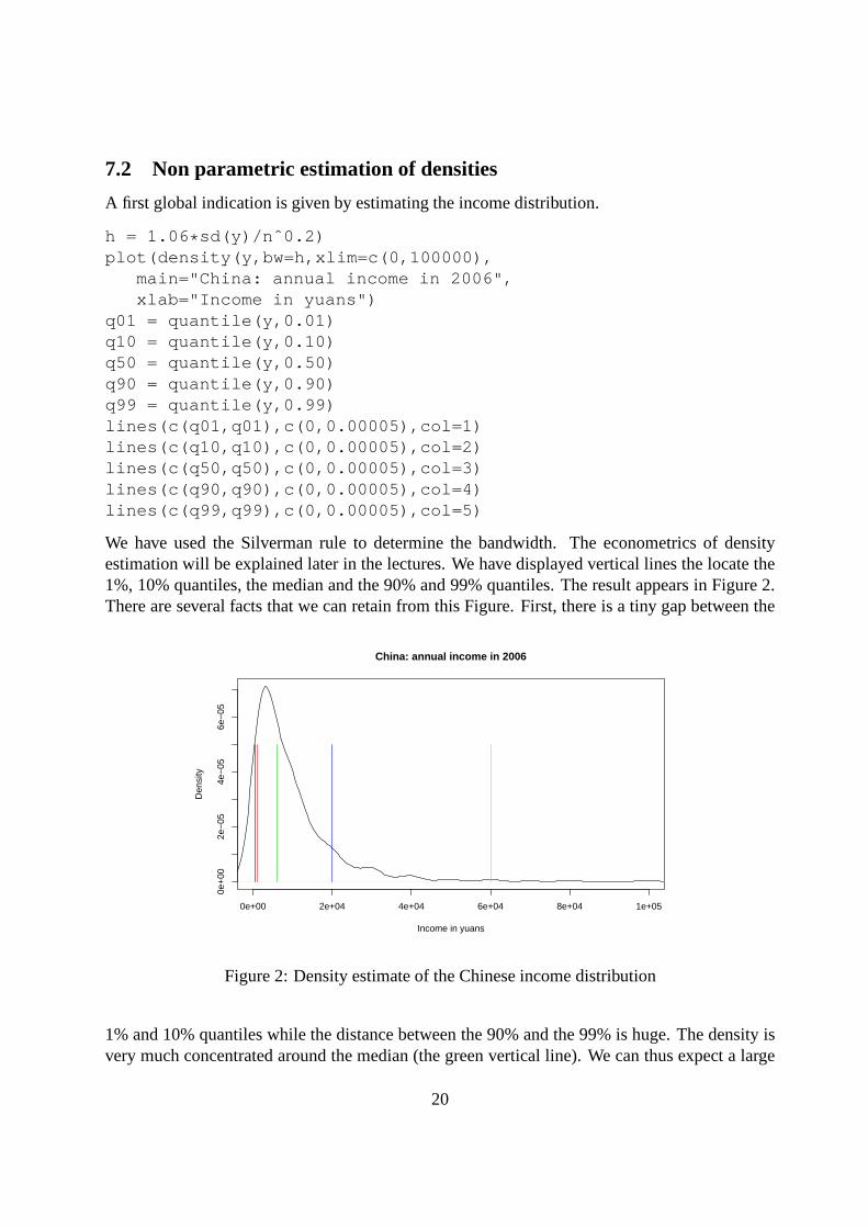
A first global indication is given by estimating the income distribution.

h = 1.06 * sd(y)/nˆ0.2)plot(density(y,bw=h,xlim=c(0,100000),

main="China: annual income in 2006",xlab="Income in yuans")

q01 = quantile(y,0.01)q10 = quantile(y,0.10)q50 = quantile(y,0.50)q90 = quantile(y,0.90)q99 = quantile(y,0.99)lines(c(q01,q01),c(0,0.00005),col=1)lines(c(q10,q10),c(0,0.00005),col=2)lines(c(q50,q50),c(0,0.00005),col=3)lines(c(q90,q90),c(0,0.00005),col=4)lines(c(q99,q99),c(0,0.00005),col=5)

We have used the Silverman rule to determine the bandwidth. The econometrics of densityestimation will be explained later in the lectures. We have displayed vertical lines the locate the1%, 10% quantiles, the median and the 90% and 99% quantiles. The result appears in Figure 2.There are several facts that we can retain from this Figure. First, there is a tiny gap between the

0e+00 2e+04 4e+04 6e+04 8e+04 1e+05

0e+

002e

−05

4e−

056e

−05

China: annual income in 2006

Income in yuans

Den

sity

Figure 2: Density estimate of the Chinese income distribution

1% and 10% quantiles while the distance between the 90% and the 99% is huge. The density isvery much concentrated around the median (the green vertical line). We can thus expect a large

20

inequality in this very asymmetric distribution. In order to get a realistic gap, we were obligedto discard the part of the graph which was greater than 100 000yuans, which means the partbetween 100 000 and 250 000 yuans.

7.3 Inequality measures

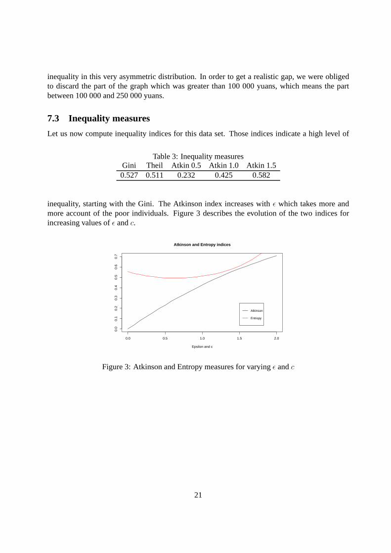
Let us now compute inequality indices for this data set. Those indices indicate a high level of

Table 3: Inequality measuresGini Theil Atkin 0.5 Atkin 1.0 Atkin 1.50.527 0.511 0.232 0.425 0.582

inequality, starting with the Gini. The Atkinson index increases withε which takes more andmore account of the poor individuals. Figure 3 describes theevolution of the two indices forincreasing values ofε andc.

0.0 0.5 1.0 1.5 2.0

0.0

0.1

0.2

0.3

0.4

0.5

0.6

0.7

Atkinson and Entropy indices

Epsilon and c

Atkinson

Entropy

Figure 3: Atkinson and Entropy measures for varyingε andc

21

The code for plotting this Figure is as follows:

nk = 25At = rep(0,nk)En = rep(0,nk)e = seq(0,2,length=nk)for (i in 1:nk){

At[i] = Atkinson(y,parameter=e[i])En[i] = Entropy(y,e[i])

}

plot(e,At,type="l",main="Atkinson and Entropy indices" ,xlab="Epsilon and c",ylab="")lines(e,En,col=2)legend(1.50,0.25,

legend=c(" ","Atkinson","", "Entropy"," "),col=c(0,1,0,2,0), lty=1:1, cex=0.9)

Note the different code which was used for the legend. The command entropy gave errors. Sowe reprogrammed it.

Entropy = function(y,c){n = length(y)mu = mean(y)if (c==0){En = mean(-log(y/mu))}else if(c==1){En = mean(y/mu * log(y/mu))}else {En = mean((y/mu)ˆc-1)/c/(c-1)}return( En)

}

7.4 Poverty measures

In China, like in India or in the Philippines, it is importantto distinguish between rural and urbanwhen analysis poverty. For instance, in December 2011 Indiafixed the urban poverty line at INR32 (USD 0.60, EUR 0.46) per day per capita and to INR 26 in ruralareas.

In 2011 China has raised the official rural poverty line to 2,300 yuan a year which makesaround $400 which makes around $1.10 a day to be compared to the World Bank internationalpoverty line of $1.25 at 2005 prices. Chen and Ravallion (2008) analyze the evolution of povertyin China before that revision and indicate a poverty line varying from 600 to 1400 yuans per yearper capita, depending on the provinces, to take into accountdifferences in prices.

The fact of being classified as urban or rural is determined inChina by the Hukou system. Inthe CGSS survey the variableqa03aindicates that status. Whenqa03a = 1, the individual has arural status, whenqa03a = 3, he is classified as urban. An other status corresponds toqa03a = 2.For individuals that have a positive income, we have the following statistics, reported in Table

22

Table 4: Income statistics by Hukou statusStatus Pop % Min Q25 Q50 Mean Q75 MaxRural 50 60 2 000 3 000 6 111 7 000 250 000Other 3 720 6 000 10 000 12 630 18 000 100 000Urban 47 20 6 000 10 000 13 980 17 000 200 000Total 100 20 3 000 6 000 9 972 12 000 250 000

5. We see that Urbans and Others have very similar characteristics. So we can join the twocategories and keep only the distinctionrural versusurban.

rural = qa03a[id]==1urban = qa03a[id]==3other = qa03a[id]==2table(qa03a[id])/nsummary(y[rural])summary(y[other])summary(y[urban])urban = (qa03a[id]==3)|(qa03a[id]==2)

We are now faced to the choice of a poverty line. There is the new official poverty line of2 300 yuans which corresponds to 77% of the median rural income or to 38% of the average ruralincome. The alternative is to consider a relative poverty line, which is more adapted for urbanareas. The usual practice (see e.g. Atkinson 1998) is to takeeither 50% of the mean income,which makes here 4 986 or 60% of the median income, which makeshere 3 600.

z1 = 2300z2 = 0.6 * median(y)z3 =0.5 * mean(y)z = c(z1,z2,z3)for (i in 1:3){cat(Foster(y[rural],z[i], parameter = 1),"")

cat(Foster(y[rural],z[i], parameter = 2),"")cat(Sen(y[rural],z[i]),"")

cat(SST(y[rural],z[i]),"")cat(Watts(y[rural],z[i]),"\n")

}

Table 5 clearly shows the importance of a correct poverty line, and the huge difference be-tween rural and urban areas. The second fact is that the two relative lines do not give the samepoverty rates: the poverty line based on the median is lower than that based on the mean. This isdue to the very large asymmetry on the income distribution inChina and implicitly to the largeinequality.

23

Table 5: Poverty measures by Hukou statusStatus P-line H.C. FGT Sen SST WattsRural

Official 0.388 0.160 0.214 0.279 0.25360% Med 0.531 0.269 0.341 0.433 0.457

50% mean 0.617 0.358 0.437 0.543 0.648Urban

Official 0.054 0.021 0.029 0.042 0.03360% Med 0.096 0.041 0.054 0.080 0.067

50% mean 0.162 0.068 0.091 0.128 0.111Total

Official 0.223 0.092 0.122 0.169 0.14460% Med 0.316 0.156 0.199 0.277 0.264

50% mean 0.392 0.214 0.268 0.366 0.382

Finally, what is the poverty rate in China. It has dropped a lot in the recent years. However,we note that the rate (Head Count) is still very important in rural areas. It is comparable to OECDrates for urban areas (between 10% and 16% using a relative poverty line). At the country scale,poverty remains relatively high, due to the weight of rural areas.

24

8 Exercises

8.1 Computing limits

Consider two functionsf(x) andg(x) andx0 such thatf(x0) = g(x0) = 0. The limit limx→x0f(x)/g(x)

is not defined. However. L’Hospital rule give a solution to remove this indeterminacy. The rulesays that it is equivalent to compute the limit oflimx→x0

f ′(x)/g′(x) wheref ′(.) is the first orderderivative. Using this rule, gives the expression of

• the generalized entropy forc = 0 andc = 1

• the Atkinson index forε = 1

• the Atkinson welfare function forε = 1

8.2 Properties of indices

• Show that the range of the Atkinson index is [0,1].

• Detail the relation between the income gap ratio and theP1 index of FGT.

• Show that forc = 2 the GE coefficient is equal to the coefficient of variation.

8.3 Poverty indices

The Sen-Shorrocks-Thon index has several expressions, which are more or less manageable. Theusual way for computing the index is

SST =1

n2

q∑

i=1

z − x[i]

z(2n− 2i+ 1).

Let us define the variable Let us define the variable

xi =z − xi

z1I(xi < z).

• Show that the SST index can take a very simple form

SST = µ(x)(1 +G(x)).

• Show that the SST index can also be written asH I(1 +G(x)).

• What is the difference between this index and the Thon index given by

Th =2

(n+ 1)n z

q∑

i=1

(z − x[i])(n+ 1− i).

• Show that the SST index is asymptotically equivalent to the Thon index when the samesample is replicated an infinite number of times.

25

8.4 Decomposable poverty indices

A poverty indexP is decomposable if it can be written as a weighted sum of partial indices.More precisely, letx = (x1, x2) and letn1 andn2 be the respective sizes of the subsamplesx1

andx2. ThenP is decomposable ifP = n1

nP1 +

n2

nP2.

• Show that the Watts index

PW =1

n

q∑

i=1

(log(z)− log(x(i))

is decomposable.

• Show the headcount measure is decomposable.

8.5 Empirics

Explore the softwareR and load the libraryineq. In this library there is a data base comingfrom the Philippines and calledIlocos. Describe this data base (help(”Ilocos”) ). Draw the Pen’sparade corresponding to this data set. Explain your results.

Use the previous data base to decompose poverty between urban and rural regions in thePhilippines.

References

Atkinson, A. (1970). The measurement of inequality.Journal of Economic Theory, 2:244–263.

Atkinson, A. (1987). On the measurement of poverty.Econometrica, 55:749–764.

Atkinson, A. (1998).Poverty in Europe. Blackwell, Oxford.

Atkinson, A. (2003). Income inequality in oecd countries: Data and explanations. WorkingPaper 49: 479-513, CESifo Economic Studies, CESifo.

Atkinson, A. B. and Bourguignon, F. (2001). Poverty and inclusion from a world perspective.In Stiglitz, J. E. and Muet, P.-A., editors,Governance, Equity and Global Markets. OxfordUniversity Press.

Chen, S. and Ravallion, M. (2008). China is poorer than we thought, but no less successful in thefight against poverty. Technical Report WPS 4621, The World Bank Development ResearchGroup.

Cowell, F. (1995).Measuring Inequality. LSE Handbooks on Economics Series. Prentice Hall,London.

26

Deaton, A. (1997).The Analysis of Household Surveys. The John Hopkins University Press,Baltimore and London.

Donaldson, D. and Weymark, J. (1980). A single-parameter generalization of the gini indices ofinequality.Journal of Economic Theory, 22(1):67–86.

Foster, J., Greer, J., and Thorbecke, E. (1984). A class of decomposable poverty measures.Econometrica, 52:761–765.

Foster, J. E. and Ok, E. A. (1999). Lorenz dominance and the variance of logarithms.Economet-rica, 67(4):901–907.

Im, D.-K. (2014).Attitudes and Beliefs about Distributive Justice in China. PhD thesis, HarvardUniversity.

Jenkins, S. P. and Lambert, P. J. (1997). Three Is of poverty curves, with an analysis of UKpoverty trends.Oxford Economic Papers, 49(3):317–327.

Okun, A. (1975).Equality and Efficiency: The Big Tradeoff. The Brookings Institution, Wash-ington (D.C.).

Piketty, T. (2017).Capital in the Twenty-First Century. Harvard University Press.

Piketty, T., Yang, L., and Zucman, G. (2017). Capital accumulation, private property and risinginequality in China, 1978-2015. Technical Report Working Paper 23368, NBER.

Rawls, J. (1971).A Theory of Justice. Oxford University Press, London.

Sen, A. (1976a). Poverty: an ordinal approach to measurement. Econometrica, 44(2):219–231.

Sen, A. (1976b). Real national income.Review of Economic Studies, 43:19–39.

Sen, A. K. (1997).On Economic Inequality. Clarendon Press, Oxford, expanded edition with asubstantial annexe by j. e. foster and a.k. sen. edition.

Shorrocks, A. F. (1995). Revisitng the sen poverty index.Econometrica, 63(5):1225–1230.

Thon, D. (1979). On measuring poverty.Review of Income and Wealth, 25:429–440.

Watts, H. (1968). An economic definition of poverty. In Moynihan, D., editor,On UnderstandingPoverty. Basic Books, New-York.

Xun, Z. and Lubrano, M. (2017). A bayesian measure of povertyin the developing world.Reviewof Income and Wealth, pages n/a–n/a.

Zheng, B. (1997). Aggregate poverty measures.Journal of Economic Surveys, 11(2):123–162.

27