the early history of the box diagram/media/richmondfedorg/publications/... · the early history of...

The Early Historyof the Box Diagram

Thomas M. Humphrey

Economists hail it as “a powerful tool,” “a work of genius,” and “oneof the most ingenious geometrical constructions ever devised in eco-nomics.” It graces the pages of countless textbooks on price theory,

welfare economics, and international trade. It is associated with some of thegreatest advances ever made in economic theory. It elegantly depicts the twofundamental welfare theorems that are absolutely central to modern economics.In short, it ranks with the preeminent schematic devices of economics since itilluminates the most important ideas economists have to offer. It is none otherthan the celebrated box diagram used to illustrate efficiency in exchange andresource allocation in hypothetical two-agent, two-good, two-factor models ofgeneral economic equilibrium.

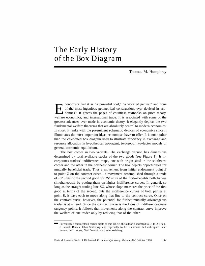
The box comes in two variants. The exchange version has dimensionsdetermined by total available stocks of the two goods (see Figure 1). It in-corporates traders’ indifference maps, one with origin sited in the southwestcorner and the other in the northeast corner. The box depicts opportunities formutually beneficial trade. Thus a movement from initial endowment point Eto point Z on the contract curve—a movement accomplished through a tradeof ER units of the second good for RZ units of the first—benefits both traderssimultaneously by putting them on higher indifference curves. In general, solong as the straight trading line EZ, whose slope measures the price of the firstgood in terms of the second, cuts the indifference curves of both parties atpoint E, it pays each to move along that line to the contract curve. Once onthe contract curve, however, the potential for further mutually advantageoustrades is at an end. Since the contract curve is the locus of indifference-curvetangency points, it follows that movements along the contract curve improvethe welfare of one trader only by reducing that of the other.

For valuable comments on earlier drafts of this article, the author is indebted to D. P. O’Brien,J. Patrick Raines, Tibor Scitovsky, and especially to his Richmond Fed colleagues PeterIreland, Jeff Lacker, Ned Prescott, and John Weinberg.

Federal Reserve Bank of Richmond Economic Quarterly Volume 82/1 Winter 1996 37

38 Federal Reserve Bank of Richmond Economic Quarterly

Figure 1 Exchange Box Diagram

SecondTrader’s Origin

FirstTrader’s Origin

Good 1

E

R Z

ContractCurve

Price Line

AutarkyIndifference

Curves

EndowmentPoint

+

01

02

Bo th t r ade rs p re fe r a l l oca t i ons i n t he shaded a rea to i n i t i a l endowmen t E .Movement down the pr ice vector connect ing endowment point E to ef f ic iencypoint Z on the contract curve puts both t raders on h igher indi f ference curvesand thus makes them be t te r o f f . A t po in t Z, however , a l l potent ia l mutual lybenef ic ia l t rades are at an end. Movements a long the contract curve benef i tone trader only at the cost of hurting the other.

The alternative production variant of the box depicts the fabrication of twogoods from two factor inputs. It replaces indifference maps representing pref-erence functions with isoquant maps representing production functions. It letsavailable factor quantities determine the dimensions of the box. Efficient factorallocations occur along the contract-curve efficiency locus. There, isoquants aretangent to each other such that the output of one good is maximized given theoutput of the other.

The chief appeal of the box diagram is its ability to explain much withlittle. A simple plane diagram, the box can, in Kelvin Lancaster’s words, “showthe interrelationships between no less than twelve economic variables” ([1957]1969, p. 52). Moreover, it can do so without resort to algebra and calculus,techniques inaccessible to the mathematically untrained. Small wonder thateconomists extol the analytical and pedagogical properties of the box or thattextbooks feature it as an expository device.

Where some textbooks go astray, however, is in their ahistoric presentationof the diagram. Typically, they say little or nothing about its origins and evolu-

T. M. Humphrey: Early History of the Box Diagram 39

tion. They simply present it as an accomplished fact without inquiring into itsgenealogy. A leading international trade theory textbook authored by RichardCaves and Ronald Jones (1981) provides a prime example. It attributes the boxto no progenitor, not even to Francis Edgeworth or Arthur Bowley. The resultis that the student is unaware of the circumstances prompting the diagram’sdevelopment. He knows not who invented it, why it was invented, what prob-lems it originally was designed to solve, or how it evolved under the impact ofattempts to perfect it and extend its range of application. Nor can he appreciatethe intellectual effort involved in its creation and refinement. Unaware of suchmatters, he may surmise that the diagram sprang fully developed from the brainof the latest theorist. Ahistoric textbooks indeed foster that very impression.Such are the hazards of disassociating an idea from its historical context andpresenting it as a timeless truth.

Far from being timeless, the box diagram possesses a definite chronol-ogy. That chronology features some of the leading names in neoclassical andmodern economics. Francis Edgeworth, Vilfredo Pareto, A.W. Bowley, TiborScitovsky, Wassily Leontief, Kenneth Arrow, Abba Lerner, Wolfgang Stolper,Paul Samuelson, T. M. Rybczynski, and Kelvin Lancaster all contributed to thediagram’s development.

Edgeworth invented the exchange box in 1881. He used it to demonstratethe indeterminacy of isolated barter and the determinacy of competitive equi-librium. He showed that all final settlements are on the contract curve, thatthe competitive equilibrium is one such settlement, and that the contract curveshrinks to the competitive equilibrium as the number of traders increases. Paretoin 1906 demonstrated his celebrated optimality criterion with the aid of thebox. Bowley in 1924 generalized Edgeworth’s work with his notion of thebargaining locus. Scitovsky in 1941 employed the box to formulate his famousdouble-bribe test of increased efficiency. Leontief coordinated, consolidated,and clarified the earlier accomplishments in his 1946 rehabilitation of the ex-change box. In so doing, he paved the way for the post-war popularity of thediagram. Following hard on Leontief’s heels, Arrow in 1951 employed theconcepts of convex sets and supporting hyperplanes to analyze the problem ofcorner solutions on the boundary of the box. And Samuelson in 1952 employedthe box to investigate how international transfers affect the terms of trade.

When the foregoing contributions threatened to exhaust the analytical po-tential of the exchange box, economists turned to the alternative productionversion. Already, Lerner had presented the first production box in a pioneering1933 paper whose publication unfortunately was delayed for nineteen years.In the meantime, Stolper and Samuelson published the first production boxdiagram to appear in print. As employed by them in 1941, by Rybczynski in1954, and by Lancaster in 1957, the production diagram proved indispensableto the derivation and illumination of certain core propositions of the emergingHeckscher-Ohlin theory of international trade.


The paragraphs below attempt to trace this evolution and to identify spe-cific contributions to it. Besides unearthing lost or forgotten insights, such anexercise may serve as a partial antidote to the textbooks’ ahistorical treatmentof the diagram. One conclusion emerges: namely that the box hardly developedautonomously. Rather it evolved in a two-way interaction with its applications.Thus an unsolved puzzle in microeconomics prompted the invention of thebox—a prime example of a seemingly intractable problem inducing the verytool required for its solution. The resulting availability of the diagram thenspurred economists to find new applications for it. These new uses in turn trig-gered modifications of the diagram. Applications were both cause and effectof the diagram’s development.

1. FRANCIS Y. EDGEWORTH

The box diagram makes its first appearance on pages 28 and 113 of FrancisEdgeworth’s 1881 Mathematical Psychics. Motivated by a problem in micro-economic theory, Edgeworth invented the diagram and its constituentindifference-map and contract-curve components to solve the problem.

Edgeworth’s predecessors had long known that equilibrium price in iso-lated, two-party exchange is indeterminate. They also understood that equilib-rium between numerous buyers and sellers operating in competitive markets isdeterminate. But they had been unable to reconcile the two results. They couldnot show rigorously how increasing numbers lead to price determinacy.

This task Edgeworth sought to accomplish. Using the box diagram, heestablished (1) that final outcomes must be on the contract curve, (2) that thecontract curve shrinks as the number of competitors increases, (3) that com-petitive equilibrium is one point on the contract curve, and therefore (4) thatas the number of competitors increases without limit the contract curve shrinksto a single point, namely the competitive equilibrium.1 Here was his rationalefor inventing the diagram.

Edgeworth’s Invention and its Components

Edgeworth’s diagram depicts two isolated individuals, A and B, trading fixedstocks of two goods, x and y, whose quantities determine the dimensions of thebox (see Figure 2). Individual A initially holds the entire stock of good x andindividual B the entire stock of good y. Superimposing indifference maps onthe box, Edgeworth sites the origin of A’s map in the lower right corner andthe origin of B’s map in the upper left corner. This arrangement fixes point 0

1 In the case of multiple competitive equilibria, the contract curve shrinks not to one but toseveral points. Edgeworth recognized such a possibility. But he tended to focus on the case ofsingular rather than multiple equilibrium. See Newman (1990, p. 261).


Figure 2 Edgeworth’s Version of the Box

M

C

PriceRay

B’s Origin

A’s Origin

C

N

0 Good x

OfferCurves

EndowmentPoint

AutarkyIndifferenceCurves

ContractCurve

IB0

0I

OA

OB

E d g e w o r t h ’ s o r i g i n a l d i a g r a m d e p i c t s t h r e e c o m p o n e n t s : ( 1 ) a u t a r k yindifference curves going through the endowment point and defining the cigar-shaped a rea o f mu tua l l y advan tageous t rades ; (2 ) o f fe r cu rves o r se ts o fpoints of tangency of indif ference curves and the price ray as i t swings aboutthe endowment point; and (3) the contract curve, whose relevant segment l iesbetween the autarky indifference curves.

+

A

in the lower left corner as the endowment point of both individuals. That is,the length of the lower horizontal axis measured from right to left indicates theamount of good x held by A just as the length of the left vertical axis measuredfrom top to bottom indicates the amount of good y held by B. Since A holdsno y nor B any x, these axes establish the endowment point.

From the indifference curves radiating outward from their respective ori-gins, Edgeworth selects one particular curve for each trader, namely the curvespassing through the endowment point. These curves show alternative combi-nations of goods that yield the same satisfaction as the endowment bundle.They indicate the level of utility each person would enjoy if he consumed his


endowment bundle and refrained from exchange. They also trace out the zoneof mutually beneficial exchanges that make both traders better off than theywould be under autarky.

Next, Edgeworth draws in the contract curve CC′ along which indifferencecurves are tangent such that one trader cannot occupy a higher indifferencecurve unless the other is forced to occupy a lower one. Especially significant isthe portion of the contract curve bounded by the autarky indifference curves.Since traders require that potential exchanges make them at least as well offas they would be under autarky, they will never voluntarily agree to tradesoutside those bounds. It follows that the relevant segment of the contract curvelies in the lens-shaped area between the indifference curves going through theendowment point.

Finally, Edgeworth sketches traders’ reciprocal demand schedules or offercurves. These curves apply to the special case where the two traders act asrepresentative price-takers operating on opposite sides of a competitive mar-ket. Offer curves show how much each trader is willing to exchange at allpossible prices. Edgeworth of course did not invent such curves. That honorgoes to Alfred Marshall. But he was the first to derive them as the locus ofpoints of tangency of indifference curves and the price ray as it pivots aboutthe endowment point. He likewise was the first to explain that each point onan offer curve represents an outcome of constrained utility maximization inwhich the commodity price ratio, or slope of the price ray, equals the ratio ofmarginal utilities, or slope of the indifference curves.

Exploiting Potential Mutual Gains from Exchange

Having derived the exchange box and its constituent components, Edgeworthemployed it to illuminate five basic propositions. His first proposition states thatfinal settlements must be on the contract curve. At any other point, both partiescould make themselves better off by renegotiation. Consider any point lying offthe contract curve. Going through that point are intersecting indifference curvesenclosing a cigar-shaped area that spells unexploited potential mutual gainsfrom exchange. Traders will not let such opportunities go unrealized. Instead,they will exploit them until they reach the contract curve where indifferencecurves are tangent and further mutual gains are at an end.

Efficiency of Competitive Equilibrium

Edgeworth’s second proposition refers to the efficiency of competitive equi-librium. It states that such equilibrium is always on the contract curve. Thereason? Competition establishes a common, market-clearing price ratio.Competitive price-takers independently respond to that ratio by trading at thepoint where each supplies the quantity the other demands and vice versa.That is, price-takers operate at the point where their offer curves intersect (see


Figure 3 Competitive Equilibrium versus the Indeterminacyof Two-Party Barter

Competit iveEquil ibrium

M

C

OfferCurves

P r i c eRay

C

N

Bestfor A

Bestfor B

B’s Origin

Good x A’s Origin0

IB0

IA0

OA

OB

Bargaining between two isolated traders can lead to an outcome anywhere onthe segment of the contract curve between the autarky indifference curves. Bycontrast, the competit ive equil ibrium is uniquely determined at the intersectionof the pr ice ray and of fer curves. There the t raders ’ ind i f ference curves aretangent to the common price ray and thus to each other.

+

Figure 3). At this point, indifference curves are tangent to the common priceray emanating from the endowment point and thus are tangent to each other.Since such tangencies occur only on the contract curve, it follows that com-petitive equilibrium is on that same curve.

Indeterminacy of Isolated Two-Party Barter

Edgeworth’s third proposition refers to the indeterminacy of isolated two-partyexchange. In such bilateral monopoly situations, it is impossible to determine,from indifference maps and endowments alone, the precise price-quantity equi-librium that will emerge. All one can say is that equilibrium must lie on the


segment of the contract curve between the autarky indifference curves. Butwhich one of the infinity of possible equilibria will prevail will depend uponconsiderations external to Edgeworth’s model, namely the relative bargainingskills and strengths of the traders as well as the strategies and tactics theyemploy. Economists traditionally have had little to say about such matters.2

They cannot confidently predict any unique outcome. The precise ingredi-ents of shrewd, effective bargaining remain subtle, elusive, and obscure. Still,economists can note that the gain one bargainer gets from exchange is limitedonly by the other’s effort to get the best for himself. Final settlement will benear point N if A is the superior bargainer. It will be nearer to point M if B hasthe bargaining advantage.

Neither outcome, Edgeworth noted, necessarily coincides with the pointof maximum aggregate welfare on the contract curve. There the sum of thetraders’ satisfactions is at its peak. Identifying this unique maximum point ofcourse requires that utility be cardinally measurable and comparable acrossindividuals—properties Edgeworth thought utility possessed. It was on thesegrounds that he advanced his famous principle of arbitration. Compulsoryarbitration, he argued, could do what unrestricted bargaining could not do.By imposing the utilitarian sum-of-satisfactions solution on the bilateral mo-nopolists, arbitration would yield a determinate, socially optimum outcome.Conversely, in the absence of such arbitration indeterminacy would continueto characterize the isolated two-party case.

Recontracting and the Role of Numbers

Edgeworth’s fourth proposition, his recontracting theorem, refers to the role ofnumbers in reducing indeterminacy. It states that as the number of traders getslarge, the contract curve shrinks to a single point, the competitive equilibrium.

Edgeworth sketches a proof on pages 35–37 of his Mathematical Psychics(see Creedy [1992], pp. 158–65, for a particularly clear and insightful inter-pretation). He starts with the two-person case in which party A provisionallycontracts with party B to reach point C on A’s indifference curve IA0

(see Figure4a). He then introduces a new pair of traders identical to the first pair. This

2 They have said something, however. John Nash (1950) thought the bargainers might agreeto maximize the multiplicative product of their respective utility gains from trade (the excessof post-trade over autarky levels of satisfaction). John Harsanyi (1956) showed that the Danisheconomist Frederick Zeuthen (1930) had proposed essentially the same solution two decadesbefore Nash. Ariel Rubinstein (1982) showed that the Nash solution is the outcome of a non-cooperative, offer-counteroffer game. John Creedy (1992, pp. 193–99) suggested a variant ofthe Nash solution, namely the maximization of a geometrical weighted average of the traders’utility gains, with the weights measuring the relative bargaining powers of the two parties. Thesesolutions establish unique potential agreement points on the contract curve. Since it is unlikelythat the bargainers would always agree to go to such proposed points, however, indeterminacyremains.


Figure 4 Edgeworth’s Recontracting Process

+

ba

dc

0

0

0

C

CP

0

C

C1

C

P1

IB0

IA0

IB0

IA0

IAIA

1 2

3

C

C*

CP*

IB0

IA0IA

IB

0IA

0

C

C

P

Recontract ing plus convexi ty of indi f ference curves impl ies that the contractcurve shrinks as traders become more numerous. With a single pair of traders,the contract curve is CC' as shown in panel a. Adding another pair shrinks thecurve by the amount CC * a t bo th ends (pane l c ) . When the number o f pa i rsgets very large, the curve shrinks to the competit ive equil ibrium (panel d).

maneuver allows him to use the same box diagram to deal with four parties. Itpermits him to represent the preferences of each of the As (and the Bs) with asingle indifference map.

It also means that the agreement reached at point C cannot be final. Forthe two As can now ignore one of the Bs and deal with the other at point C.When they split the resulting bundle equally among themselves, they will eachreach the half-way point P on the trade vector 0C. That point, because of theconvexity of indifference curves, is on a higher such curve than before. Thusthe As are better off, their trading partner B is just as well off as initially, andthe excluded B is at his endowment point.


In retaliation, the excluded B then underbids his competitor by offering theAs a trade on better terms at point C1 (see Figure 4b). The As, by accepting, canshare the resulting bundle among themselves to each attain point P1 on a stillhigher indifference curve than before. Repeated recontracting brings the partiesto point C∗ (see Figure 4c). There the As are indifferent between (1) trading withboth Bs at C∗ and (2) dealing with just one B at C∗ and splitting the resultingbundle at point P∗. Either option puts them on the same indifference curve.

There being no advantage to choosing option 2 over option 1, the As willtrade with the two Bs at point C∗. The result is that recontracting, which beganat point C, ends at point C∗. Adding a trader to each side of the market shrinksthe contract curve by the amount CC∗. The same logic of course applies topoint C′ at the other end of the contract curve. Recontracting initiated thereshrinks the contract curve inward as each of the As continually underbids theother to attract the business of the Bs. In other words, the contract curve shrinksat both ends.

Although two pairs of traders shrink the range of indeterminacy, they hardlyeliminate it. To reduce it further, Edgeworth adds a third pair. Doing so givesroom for two Bs to underbid the third for the patronage of the As. Dealing withthe two Bs, the three As each can reach a point P two-thirds the distance fromthe origin to any point C on the contract curve. Final settlement occurs whenpoint C shrinks inward sufficiently to lie on the same A-indifference curve aspoint P. The same reasoning holds for the other end of the contract curve,which of course shrinks too.

Let the number of pairs of traders N grow without limit. Then point P,which according to Edgeworth is (N − 1)/N times the distance from the originto point C, converges on that latter point. Expressed geometrically, final settle-ment in the large-numbers case occurs where an A-indifference curve is tangentto a ray from the origin (see Figure 4d). The same holds true for an indifferencecurve of the Bs. The result is that both indifference curves are tangent to thesame ray and thus to each other just as in the competitive equilibrium. Largenumbers shrink the contract curve to the point of competitive equilibrium.

Monopoly Pricing—An Exception to Edgeworth’s Rule?

Finally, Edgeworth considered a case that apparently violated his postulate thatfinal settlements lie on the contract curve. That case has two bargainers agreeingon price but making no agreement on the quantities to be traded. An extremeexample confronts a representative competitive price-taker with a monopolisticprice-maker. The monopolist is of the simple, or non-price-discriminating,variety. He sets a single price for all units exchanged and leaves the competitorfree to determine how much he (the competitor) wants to trade at that pricealong his offer curve.

Let A be the representative competitor and B the monopolist. If B’s monop-oly power is absolute, he will set the single price that puts him on his highest


attainable indifference curve given A’s offer curve (see Figure 5). That is, hechooses the price that takes him to point Q, where his indifference curve justtouches A’s offer curve. Of course, if his monopoly power is less than absolute,his fear of losing A’s patronage to potential rival traders may induce him tocharge the slightly lower price shown by the slope of ray 0q. In any case, theresult is that trade takes place at a point like Q (or q) on A’s offer curve ratherthan on the contract curve. Here is an apparent exception to the rule that finalsettlements tend to be efficient.

Edgeworth was quick to point out, however, that the exception stems fromthe assumption that the parties contract over price alone. Were they to contractover quantity as well, they both could move advantageously to the contractcurve. Thus Edgeworth questioned the validity of the assumption. To him,rational behavior required that parties bargain over both price and quantitydimensions of a deal, especially when it was to their mutual advantage todo so.

In illustration, Edgeworth referred again to monopoly point Q reachedthrough a price-only contract. From that point, superior outcomes are possiblein the sense that both parties can move to higher indifference curves thanthose crossing through Q. Edgeworth realized, however, that such improvedpositions would never be attained by new price settings alone. For, given thatthe monopolist is constrained by the competitor’s offer curve, any change in theslope of the price line 0Q would make him (the monopolist) worse off than heis at Q and for that reason would be resisted. But mutually beneficial positionscould be reached if the competitor somehow could be induced to leave his offercurve. Such an inducement could take the form of a new contract specifyingquantity as well as price.

For example, monopolist B might dictate terms corresponding to point Z,thus improving his own welfare. He would lower the price against himself inexchange for a more-than-compensating rise in quantity traded. And he woulddo so confident that A would gladly agree to the larger trade volume in returnfor the guarantee of a lower price. In other words, A would concur with anyprice-quantity package moving him to an indifference curve higher than theone he would otherwise occupy at point Q. And if such a negotiated packagefell short of the contract curve, the parties could renegotiate other packagesuntil they finally arrived there.3

3 Tibor Scitovsky, in his classic 1942 article “A Reconsideration of the Theory of Tariffs,”showed that the parties could reach point Z by an alternative route. Competitor A could bribemonopolist B to act as a competitor operating on his own offer curve. The bribe, paid in A’s owngood, would result in a rightward shift of the endowment point and its attendant offer curvesby the amount of the payment. So shifted, the offer curves would intersect at point Z. Themonopolist would gain from the bribe and the price-taker would gain from the lower, competi-tive price. Edgeworth, however, said nothing of this scheme.


Figure 5 Monopoly Outcomes

A’sOfferCurve

Q

B’s OfferCurve (were he

not a Monopolist)

ContractCurve

BetterPoint

B’sMonopoly

Point

B’sMonoplyIndifferenceCurve

A’s IndifferenceCurveat the

MonopolyPoint

q

MonopolyPriceLine

+

Z

OA

OB

0

Monopol is t B se t s t he p r i ce t ha t pu t s h im on h i s h ighes t a t t a i nab le i nd i f -f e rence cu rve g i ven the o f fe r cu rve o f t he compet i t i ve p r ice - take r A . T h emonopol ist goes to tangency point Q . There, however, A ’s indifference curvei s t angen t t o t he p r i ce ray and no t t o B ’s indi f ference curve. The resul t ingin te rsec t ing ind i f fe rence curves c rea te a lens-shaped area o f unexp lo i tedmutual ly benef ic ia l exchanges. I f the part ies could agree to let monopol ist Bset both pr ice and quant i ty , they could move to ef f ic ient point Z where bothare better off than at point Q .

Good x

In short, Edgeworth showed that agreements fixing both price and quantityinevitably lead to the contract curve. By contrast, agreements limited to es-tablishing price alone may, under certain circumstances, lead only to the offercurve. But he insisted that rational agents have an incentive to choose theformer agreements over the latter. Thus all final settlements tend to be on thecontract curve.

Appraisal

Edgeworth’s contribution must be judged one of the greatest virtuoso perfor-mances in the history of economics. Going beyond the mere creation of the


box diagram itself, he invented its principal components, the indifference mapand the contract curve. True, he did not invent offer curves. But he did givethe earliest demonstration of their derivation from the underlying indifferencecontours and price ray. Moreover, in showing that offer curves intersect at thecontract curve, he was the first to use them to demonstrate the efficiency ofcompetitive equilibrium.

Edgeworth’s work is remarkable in another respect. His five propositionsessentially point the way to all of modern economics. One finds in them both atreatment of competitive equilibrium and its efficiency in exhausting the gainsfrom trade and a framing of the problems that arise when perfect competitionceases to prevail. These problems arguably constitute the fundamental motiva-tion for the development of game theory.

Indeed, Edgeworth himself contributed to this development by anticipat-ing key game-theoretic ideas. He demonstrated that final allocations must lieon the segment of the contract curve spanning the indifference curves goingthrough the endowment point. In so doing, he identified what game theoristssome seventy-five years later were to call the core of the economy. And, inillustrating that the contract curve shrinks to a single point, he showed how thecore behaves as its agents increase in number. Finally, his recontracting theoryforeshadowed the game-theoretic notion that no coalition of traders can blockthe emergence of competitive equilibrium. Mark Blaug (1986, p. 70) said itall when he described Edgeworth’s theory of the core as “his most beautifulcontribution.”

2. VILFREDO PARETO

The next to present the box diagram was Vilfredo Pareto, who did so in his1906 Manuale d’economie politica. Pareto’s work obviously owes much toEdgeworth. Indeed, commentators including Maffeo Pantaleoni (1923, p. 584)and John Creedy (1980, p. 272) have stressed that very point. But Pareto alsomodified Edgeworth’s work in at least two key respects.

For one thing, he presented the box in its now-conventional form. That is,he located the origins of the indifference maps in the southwest and northeastcorners, respectively, rather than in the other two corners as Edgeworth haddone (see Figure 6). The result was that the succession of indifference-curvetangency points—Pareto did not draw the efficiency locus—sloped upwardfrom left to right rather than downward as in Edgeworth’s version.

Second and more important was Pareto’s interpretation of the welfareimplications of the box. Unlike Edgeworth, who believed that interpersonalcomparisons of utility make it possible in principle to identify a unique pointof maximum aggregate welfare on the contract curve, Pareto denied that suchcomparisons could be made and indeed refused to make them.


Figure 6 Pareto’s Diagram

D

B

SecondTrader’s Origin

0

E

2

3

4

1

1

2

3

4

A

FirstTrader’s Origin

0

Movements f rom point D to any point wi th in the lens-shaped areaare unambiguously wel fare- improving since both part ies gain andnei ther lose. But movements across tangency points A, E , a n d Bare welfare-ambiguous and defy comparison since one party gainswhile the other loses.

Good 1

+

Pareto Optimality

Accordingly, he held that only outcomes involving gains for some and losses fornone are unambiguously welfare-improving just as outcomes involving gainsfor none and losses for some are unambiguously welfare-decreasing. By con-trast, outcomes involving gains for some and losses for others are ambiguous.They cannot be judged in terms of quantitative utility comparisons. The inad-missibility of interpersonal comparisons of utility (or “ophelimity” as Paretotermed the utility concept) foils their evaluation.

It follows that movements from points like D, where indifference curvescross, to points like A, E, and B, where the curves are tangent, constitute


Pareto-superior moves. They put at least one party on a higher indifferencecurve and none on a lower one. But movements across successive tangencypoints like A, E, and B, involving as they do higher curves for one person andlower curves for the other, defy comparison. An infinity of such Pareto-optimalpoints exists, none of which can be judged superior to the others.

In short, there is no single point of maximum welfare, Edgeworth’s claimto the contrary notwithstanding. All one can say is that points off the tangencylocus are economically inefficient since everyone could gain by moving to apoint at which no mutually advantageous reallocations are possible. Likewise,points on the locus are economically efficient in the sense that no reallocationcould improve the position of both parties. Edgeworth’s notion of a uniquewelfare optimum gave way to Pareto’s notion of an infinity of noncomparableoptima.

3. ARTHUR W. BOWLEY

After Pareto’s Manuale, fully eighteen years elapsed before the box diagrammade its next appearance in A.W. Bowley’s famous 1924 MathematicalGroundwork of Economics. Inspired by Edgeworth and Pareto, Bowley general-ized and extended their work in three ways. First, he replaced their assumptionthat each hypothetical trader initially holds the entire stock of one good andnone of the other. He replaced it with the alternative assumption that eachtrader initially holds some of both goods. The result was to fix the endowmentpoint in the interior of the box rather that at one of its corners (see Figure 7).Bowley’s innovation is conventional practice today.

Bargaining Locus

Second, he supplemented Edgeworth’s analysis of bilateral monopoly with hisconcept of the bargaining locus. In defining that locus, which consists of theoffer-curve segments Q1QQ2, Bowley argued as follows. If the two partiescontract over price alone, equilibrium may well be on the offer curves ratherthan on the contract curve. The party possessing the superior bargaining powerwill set the price and leave the other free to determine the trade volume at thatprice along his offer curve. Accordingly, the outcome will be somewhere onthe price-taker’s offer curve.

Suppose B is the price-maker whose bargaining superiority is absolute. Hewill set the price to reach point Q2 where his highest attainable indifferencecurve just touches A’s offer curve. But if his bargaining superiority is some-what weakened by the countervailing bargaining skills of A, he will be forcedto shade his price downward and occupy a position on A’s offer curve in thedirection of competitive point Q. These considerations trace out the lower Q2Qsegment of the bargaining locus.


Figure 7 Bowley’s Version of the Box

Bargain ing between pr ice-making, pr ice- tak ing t raders establ ishes thecurve Q QQ as the locus of f ina l outcomes. F inal set t lement occurs ont h e u p p e r o r l o w e r s e g m e n t d e p e n d i n g u p o n w h e t h e r A o r B i s t h ed o m i n a n t b a r g a i n e r . I f b o t h p a r t i e s p o s s e s s e q u a l a n d o f f s e t t i n gmonopoly power, f inal sett lement occurs at Q .

C

C

+

ContractCurve

Q1

Q

Q2

R

T

B’s Origin

0 A’s OriginGood x

B’s OfferCurve

A’s OfferCurve

EndowmentPoint

21

Similarly, if A is the price-maker, trade will occur at the point of intersec-tion of the price ray he sets and B’s offer curve. Trader A will aim at reachingpoint Q1, where the offer curve is tangent to his highest attainable indifferencecurve. But if A’s bargaining power is less than absolute, he may be forced tolower the price against himself and thus move to a point on B’s offer curve tothe right of point Q1. These considerations establish the upper Q1Q segmentof the bargaining locus.

The upshot is that if either one trader or the other sets the price, tradeoccurs at some point on the combined upper and lower segments of the offer


curves between points Q1 and Q2.4 With the single exception of point Q, whereequal and offsetting bargaining power yields the competitive equilibrium, allthese points are off the contract curve. Thus Bowley confirms Edgeworth’scontention that when price-maker confronts price-taker over price alone theoutcome is rarely efficient.

Trading at Disequilibrium Prices

Finally, Bowley advanced an alternative to Edgeworth’s treatment of how theeconomy converges to its core. As mentioned above, Edgeworth, in consideringsuch convergence, ruled out trading at disequilibrium prices. For him, contractsbecome binding and exchanges occur only at final equilibrium prices corre-sponding to points on the contract curve. Disequilibrium contracts he treated astentative, provisional, non-binding, and subject to revision until the equilibriumcontract emerged.

By contrast, Bowley permitted exchanges to take place at disequilibriumprices. He envisioned traders moving across a succession of intermediate posi-tions in the lens-shaped area enclosed by indifference curves emanating fromthe endowment point. From each such intermediate trading position, they wouldmove to a subsequent, Pareto-improving one changing the price as they went.They would continue in this fashion until they reached the core. The resultingpath to equilibrium is described by a broken, or segmented, price line and finalsettlement can occur anywhere on the section RT of the contract curve.

For all its apparent realism, however, Bowley’s analysis comes at a highcost. It greatly complicates the diagram. Each disequilibrium trade means a newallocation of goods such that the endowment point shifts continually. Since offercurves emanate from such endowment points, a new set of offer curves has to bedrawn at each stage of the process. The result is to clutter the diagram unduly.For this reason, Edgeworth’s simplification seems superior pedagogically toBowley’s treatment.

4. TIBOR SCITOVSKY

In the twenty-two years following the publication of Bowley’s MathematicalGroundwork, the exchange box virtually disappeared from the literature. Itsurfaced briefly in 1941 when Tibor Scitovsky employed it to expose a flaw

4 This result holds even when both bargainers, after agreeing on a noncompetitive price,treat it as given and act as price-takers operating on their respective offer curves. In this specialcase, the price ray will cut the respective offer curves at different points. One party, in otherwords, will wish to trade a larger quantity at the bargained price than will the other. Here, thesmaller quantity will be the one actually traded. The outcome will be exactly the same as if oneparty unilaterally set the price (see Scitovsky 1951, p. 418).


in compensation tests of increased efficiency. Nicholas Kaldor and John R.Hicks had proposed such tests to circumvent Pareto’s prohibition banning theevaluation of changes favoring some people while hurting others. Applied tosuch situations, the compensation test was supposed to reveal whether a changefrom one non-optimal state to another was, on balance, welfare-improving ifsome gained and some lost. The change was said to pass the test if the gainerscould fully compensate the losers and still be better off.

But Scitovsky noted a paradox. The test might reveal both states to be su-perior to each other. Observe a change-induced reallocation from goods-bundleA to bundle B (see Figure 8). Let points A and A′ have the same verticalheight with the same being true of points B and B′. Then compensation canbe represented as a quantity of the horizontally measured good alone. GainerJ (whose indifference map originates at the lower left) could fully compensateloser I (whose indifference map originates in the upper right) by an amount B′Band still be better off. The hypothetical transfer would leave him occupyinga higher indifference curve than the one going through his initial position A.Similarly, in a reverse transition from B to A, individual I could bribe individualJ by an amount AA′ and still be better off than at B. The test would revealallocation B as preferred to allocation A. Once at B, however, the same testwould reveal A as the superior allocation.

Double-Bribe Criterion

To avoid such contradictions, Scitovsky proposed a double test. Situation B ispreferred to situation A if the gainers from the change can profitably compensatethe losers, or bribe them to accept it, while the potential losers cannot profitablybribe the gainers to oppose the change.

Scitovsky’s double-bribe criterion impressed economists far more than didthe box diagram he used to exposit it. For that reason, his paper served merely tointerrupt rather than to halt the diagram’s pre-World War II lapse into obscurity.That lapse persisted for five more years.

5. WASSILY LEONTIEF

Then came Wassily Leontief’s 1946 Journal of Political Economy article on“The Pure Theory of the Guaranteed Annual Wage Contract.” Employingperhaps the most elaborate version of the exchange box to be found in thescholarly literature of the time, Leontief summarized, consolidated, and clari-fied all earlier work. He spelled out such notions as the lens-shaped zone ofmutually advantageous trades, the contract curve, offer curves, the competitiveand simple monopoly (price-maker, price-taker) outcomes and their welfareimplications with a lucidity and elegance unmatched in earlier work. In sodoing, he reawakened economists to the power and subtlety of the diagram andthus initiated its post-war revival.


Figure 8 Scitovsky’s Paradox

+

I ’s Origin

J’s Origin

B

A A

J2

J1

I1

I2

B

J1I2

I1

J2

Paradoxical ly , the Kaldor-Hicks compensat ion test may just i fy both amove from si tuat ion A to s i tuat ion B and a reverse move f rom B backto A. In the move f rom A t o B, agent J could compensate agent I bythe amount BB ' and st i l l be better of f . He would st i l l occupy a higherindif ference curve than at A. Contrar iwise, in the reverse move from Bto A, agent I could compensate agent J by the amount AA ' and st i l l bebetter off than at B.

Good 1

Perfectly Discriminating Monopoly

Leontief’s main contribution, however, was to specify exactly how a domi-nant bargainer might extract for himself all the potential gains from trade. Letthat bargainer present his passive counterpart with an all-or-nothing, take-it-or-leave-it option to trade the entire fixed bundle C at a fixed price equal to theslope of ray 0C (see Figure 9). The passive party either accepts the option orrejects it and remains at his endowment point. Since the option leaves him noworse off than does the autarky outcome, he accepts it. The resulting settlementis at one end of the core, namely at the extreme that yields the dominant partyall the gains from exchange.


Figure 9 Perfectly Discriminating Monopolist

Trader B, a per fect ly d iscr iminat ing monopol is t , captures a l l the potent ia lgains f rom t rade for h imsel f by going to point C on h is t rading par tner A ’sautarky indif ference curve A . He presents A wi th an al l -or-nothing, take- i t -or- leave- i t opt ion to t rade the f ixed bundle C a t the f ixed pr ice denoted bythe s lope o f r ay 0C. A l ternat ive ly , B ach ieves the same resu l t by mov ingdown A ’s autarky indif ference curve, charging the highest pr ice he can getf o r each success i ve un i t o f t r ade un t i l he a r r i ves a t po in t C. Un l i ke thes imple monopoly outcome M , the d iscr iminat ing monopoly outcome is onthe contract curve and therefore is eff icient.

+

E

B1

B2

B0

MB

CMA

C

A’s Origin

EndowmentPoint B’s Origin

A’sOfferCurve

A0

A

A1

B’sOfferCurve

0

Good 1

2

0

B

Leontief further noted that all-or-nothing option contracts are equivalentto perfect price discrimination. With price discrimination, the dominant tradermoves along the autarky indifference curve of the passive trader. He does soby charging the highest price he can get for each successive unit of trade—thatis, the highest price his partner is willing to pay rather than do without theunit—until he (the dominant trader) reaches the core at a point most favorableto himself. The result, in terms of the distribution of the gains from trade, isclearly the same as that achieved by the take-it-or-leave-it option.

In stressing this point, Leontief also emphasized that price discrimination,because it leads to the contract curve, is economically efficient. Like perfect


competition, it wastes no resources. In this respect, the discriminating monopolyoutcome is preferable to the simple monopoly one.

The significance of Leontief’s contribution was this. Edgeworth and Bow-ley had stated that final settlement might occur at either extreme of the core.But they had failed to identify such outcomes with all-or-nothing options anddiscriminatory pricing. Leontief did so and established once and for all theexact price-quantity agreements that produce such outcomes.

6. OTHER POST-WAR CONTRIBUTIONS:KENNETH ARROW AND PAUL SAMUELSON

Leontief’s rehabilitation of the exchange box contributed greatly to its popular-ity in the late 1940s and early 1950s. Extensions and generalizations followedwhen Kenneth Arrow and Paul Samuelson found imaginative new uses forthe box.

Arrow, in his 1951 essay “An Extension of the Basic Theorems of Classi-cal Welfare Economics,” did at least three things. First, he introduced modernset-theoretic concepts into the box. He interpreted the relevant regions of in-difference maps as convex consumption sets and price or budget lines as theirsupporting hyperplanes. Doing so allowed him to replace local or first-orderoptimality criteria—the familiar marginal conditions—with global criteria.

Second, he employed the foregoing concepts to establish the two fundamen-tal theorems of welfare economics. Theorem one states that every competitiveequilibrium, because it occurs at a point where each agent maximizes his satis-faction given the level of satisfaction of the other, is a Pareto optimum. Theoremtwo states that every Pareto optimum, because it can be supported by a pricevector that equates supply and demand, is a competitive equilibrium. Arrowdemonstrated that both theorems hold for the standard case where indifference-curve tangencies occur in the interior of the box.

Third, he analyzed boundary optima in which interior tangencies give wayto corner solutions on the edges of the box. His analysis yielded a positiveand a negative result. The positive result was that competitive equilibria retaintheir optimality properties even when they occur on the borders of the box.His negative result was that, without extra assumptions, there may be Paretooptimal points on the boundaries that cannot possibly be equilibrium allocations(see Figure 10).

Consider point X. There agent A’s downward-sloping indifference curvemeets the corresponding curve of agent B at its peak. Clearly this is a Pareto-efficient allocation since each agent is on his highest attainable indifferencecurve given the curve of the other. Nevertheless, this optimum cannot sustainan equilibrium. For given the flatness of B’s curve at its peak, the tangentprice vector that separates the two indifference curves at X is necessarily a


Figure 10 Arrow’s Exceptional Case

Pareto-eff icient solution X contradicts the notion that optimali ty guarantees acompetit ive equil ibrium. For the horizontal, tangent price l ine separating theind i f fe rence curves a t X i nduces agent B to max im ize h is sa t i s fac t ion byremain ing a t tha t po in t . Cont rar iw ise , i t induces agent A to max imize h issat is fact ion by moving as far to the r ight as possible. The upshot is that Aand B seek incompatible al locat ions and the market fa i ls to clear.

+

A3A4

B1

A2

X

A1

B3

B20A

0BGood 1

horizontal line coinciding with the lower edge of the box. Its slope impliesa zero relative price that induces the agents to register incompatible claims.Given the zero price, B maximizes his utility by remaining at point X. Bycontrast, A maximizes his utility by moving rightward as far as possible alongthe price line, reaching ever-higher indifference curves as he goes.

The upshot is that A and B seek inconsistent allocations at the prices im-plied by corner-solution X and so the market fails to clear. Students refer tothis curiosum as Arrow’s Exceptional Case. It violates the theorem that everyPareto optimum guarantees a competitive equilibrium.5

5 The theorem holds, however, when both indifference curves possess negative slopes atboundary optima. In such cases, a downward-sloping, tangent price line can always be fittedbetween the curves. Its slope represents the market-clearing price ratio that induces both partiesto go to the optimum point.


Samuelson, in his classic 1952 Economic Journal article on “The TransferProblem and Transport Costs,” used the exchange box to determine if a trans-fer payment made by Europe to America would worsen or improve Europe’sterms of trade. According to him, the transfer shifts the endowment point to theleft and with it the offer curves and terms-of-trade ray that intersect at worldtrade equilibrium (see Figure 11). But whether the new ray is less or moresteeply sloped than the old depends on the relative marginal propensities to con-sume Europe’s export good, clothing, in both countries. If the transfer reducesEurope’s clothing consumption more than it expands America’s, the result isan excess world supply of clothing whose relative price must therefore fall.The terms of trade will turn against Europe. On the other hand, if the transfer-induced fall in Europe’s demand for its exportable good, clothing, is less thanthe rise in America’s demand for that same good, the resulting excess worlddemand for clothing will bid up its relative price. Europe’s terms of tradewill improve. The slope of the terms-of-trade ray can become either flatter orsteeper. It all depends on the relative propensities to consume.

These extensions, however, brought the evolution of the exchange box toa halt. For the combined contributions of Leontief, Arrow, and Samuelson hadvirtually exhausted the analytical potential of the diagram and left it with littlenew to do. True, it maintained its popularity in the textbooks. But it was clearto all that the exchange box had seen its heyday. By the mid-1950s, its mainuse was to illustrate established ideas rather than to generate new ones.6 Notso the alternative production variant, however. Economists were increasinglyfinding new applications for that version of the box.

7. ABBA LERNER

Already, in December 1933, Abba Lerner had drawn perhaps the earliest versionof the production box. He presented it in a term paper on factor-price equal-ization which he wrote for Lionel Robbins’s seminar at the London School ofEconomics.

Lerner’s diagram superimposes isoquant, or production indifference, mapsof two industries fully employing two factor inputs whose fixed quantitiesdetermine the dimensions of the box (see Figure 12). Each isoquant shows al-ternative factor combinations capable of producing a given level of output. Anypoint in the box represents a particular allocation of the two factors between

6 This situation, however, proved to be temporary. Unforeseen at the time was the post-1970resurrection of the box to depict Kenneth Arrow’s notion of insurance as trade in state-contingentcommodities (see Duffie and Sonnenschein [1989], pp. 584–86, and Niehans [1990], pp. 493–95).By exchanging such commodities, agents could in principle profitably insure themselves againstthe risks of unfavorable states of the world. In so doing, they could reach the contract curvewhere the allocation of risk-bearing is optimal.


Figure 11 The Transfer Problem

+

America’sOrigin

Europe’sOrigin

American Clothing

European Clothing

B

B

C

AC A

0A

0E

Before t ransfer , Europe and Amer ica t rade a long the terms-of - t radevecto r AB l i nk ing the au ta rky endowment po in t A t o the f ree - t radeequi l ibr ium point B. When Europe pays to Amer ica a t r ibu te o f AA 'uni ts of cloth, the endowment point shi f ts horizontal ly lef tward from Ato A ' . The corresponding new trade equi l ibr ium point is B '. Whetherthe post- t ransfer terms-of- t rade vector A ' B ' is s teeper or f la t ter thanthe old one depends on the countr ies’ marginal propensit ies to spendt h e p r o c e e d s o f t h e t r i b u t e o n c l o t h v e r s u s f o o d . E i t h e r r e s u l t i sposs ib le . Thus a t rans fe r can cause the pay ing coun t ry ' s te rms o ftrade to deteriorate, improve, or remain unchanged.

the production of the two goods. Isoquants going through such points showquantities of both goods produced with this factor allocation.

Regarding factor allocations off the locus of isoquant tangency points,Lerner notes that they are technologically inefficient. They squander scarceresources. They leave room for at least one industry, via mere reallocation ofexisting inputs, to increase its output with no loss of output of the other. Thus,starting from point Z, one can, by moving along isoquant B until it reachestangency with isoquant A, increase the output of good A with no decrease inthe output of good B. No such feat is possible on the efficiency locus itself,however. There, one industry’s expansion spells the other’s contraction. There,factor allocations are technologically efficient in the sense that they maximizethe output of one good given the output of the other.

Efficiency, then, requires producers to operate on the contract curve. And,according to Lerner, competition and factor mobility together ensure that they


Figure 12 Lerner’s Production Box Diagram

Factor 10A

0B

+

P

Z

A

A

B

B

At inef f ic ient point Z , good A ’ s ou tpu t can be increased w i th no loss ing o o d B ’ s o u t p u t . P r o d u c e r s s i m p l y r e a l l o c a t e f a c t o r i n p u t s t o A-production so as to move along the given B isoquant cutt ing successivelyh igher A i soquan ts in the p rocess . A t e f f i c ien t po in t P on the con t rac tc u r v e , h o w e v e r , t h e o u t p u t o f o n e g o o d c a n b e i n c r e a s e d o n l y b ydecreasing the output of the other.

will do so. Competition forces producers to hire both factors until the ratioof their marginal products, represented by the slopes of isoquants, equals theratio of their prices, represented by the slope of a relative factor-price line. Andfactor mobility dictates that resource prices, and so their ratio, are the samein both industries. Consequently, both industries operate at a point where theirisoquants are tangent to a common factor-price-ratio line and thus are tangentto each other. Such points lie on the contract curve.


Delayed Publication

Unfortunately, economists had to wait for nineteen years to see Lerner’s pio-neering diagram. Tibor Scitovsky, in his essay on “Lerner’s Contributions toEconomics,” tells why. In 1948 and 1949, Paul Samuelson published his cel-ebrated proof of the factor-price-equalization theorem. Robbins, upon readingSamuelson’s papers, recalled Lerner’s 1933 term paper on the same subject.Robbins still had a copy of the paper in his files. Upon his urging, Lerner pub-lished the manuscript without alteration as the 1952 Economica piece “FactorPrices and International Trade.”

As to why Lerner neglected to publish the paper in 1934, Tibor Scitovskyrecounted a story he heard in 1935 when he was one of Lerner’s students.Evidently, Lerner had given his only corrected copy to another student to betypewritten for submission to a scholarly journal. But the student lost the paperon a London bus and was unable to retrieve it. Lerner, who was busy writingother papers at the time, could not find the time to reproduce the lost manuscript.The resulting delay made Lerner’s pathbreaking work and its innovative dia-gram seem less-than-novel when they finally appeared. In any case, it was notfrom Lerner but from Wolfgang Stolper and Paul Samuelson that the economicsprofession first learned of the production box.

8. WOLFGANG STOLPER AND PAUL SAMUELSON

Wolfgang Stolper and Paul Samuelson published the first production box dia-gram to appear in print. It features prominently in their 1941 Review ofEconomic Studies article on “Protection and Real Wages.” Of the two authors,Stolper (1994, p. 339) credits Samuelson with the idea of using the box. In anycase, they applied it to derive their famous theorem according to which freetrade benefits the relatively plentiful factor and hurts the relatively scarce onewhile protective tariffs do the opposite.

Stolper-Samuelson Theorem

The Stolper-Samuelson theorem rests on two propositions. First, compared withautarky, free trade raises the price of the relatively abundant factor and lowersthe price of the relatively scarce one. Conversely, trade restriction raises thescarce factor’s price and lowers the plentiful factor’s. Second, it follows that atariff-induced restriction of trade may benefit labor in countries where labor isthe scarcer factor. In such countries, a tariff may raise real wages and increaselabor’s real income both absolutely and relatively as a percent of the nationalincome.

Stolper and Samuelson reached these conclusions via the following route.Suppose in the absence of trade a country produces wheat and watches with a


fixed factor endowment consisting of much capital and little labor (see Figure13). Measure capital on the horizontal axes of the box and labor on the verticalones. The box, being wider than it is tall, indicates a high ratio of capital tolabor and thus identifies capital as the relatively plentiful factor and labor asthe relatively scarce one.

Next assume that, at any given factor-price ratio, wheat production requiresa higher ratio of capital to labor than does watch production. Wheat, in otherwords, is capital intensive and watches are labor intensive. The slopes of labor-to-capital factor-proportion rays going through any point on the contract curveshow as much. Those rays are steeper for watches than for wheat. Moreover,the contract curve lies everywhere below the diagonal of the box. Were factorintensities the same in both industries, the contract curve would coincide withthe diagonal. And were factor-intensity reversals to occur, the contract curvewould cross the diagonal. Neither possibility is allowed. Both are ruled out byassumption.

Initially, in the absence of trade, the country produces and consumes atpoint M on the contract curve. Wheat, embodying relatively large amounts ofrelatively cheap and plentiful capital, is the low-cost good. Conversely, watches,embodying much scarce and hence relatively dear labor, constitute the high-cost good. Given that the opposite conditions prevail in the rest of the world,the result is that wheat is cheaper in terms of watches at home than abroad.

Free Trade Helps the Plentiful Factor

When trade opens up, foreigners will import the home country’s cheap wheatand home residents will import foreigners’ cheap watches. The consequentincreased demand for the home country’s wheat and the decreased demand forits watches bids up the domestic price of wheat relative to the price of watches.The resulting price rise induces wheat producers to expand by hiring capital andlabor from watch producers so as to move to free-trade point N. But the con-tracting watch industry, being labor-intensive, releases relatively little capitaland relatively much labor compared to the ratio in which the capital-intensivewheat industry wants to absorb those factors. The ensuing labor surplus andcapital shortage bids wages down and capital rentals up. The lower wagesand higher rentals in turn induce both industries to substitute cheaper laborfor dearer capital. The upshot is that the labor-to-capital ratio rises in bothindustries. And it does so even as the overall economy-wide endowment ratioshown by the slope of the diagonal stays unchanged. In terms of the diagram,both factor-proportion rays through point N are steeper than those throughpoint M.

With less capital working with each unit of labor in both industries, themarginal product of labor falls and the marginal product of capital rises. Undercompetitive conditions, those marginal products constitute factor real rewards


Figure 13 Stolper-Samuelson Theorem

Free t rade moves the cap i ta l - r i ch economy f rom au ta rky po in t M t o f ree - t radep o i n t N. T h e d a s h e d r a y s s h o w t h a t t h e l a b o r - t o - c a p i t a l r a t i o r i s e s i n b o t hindustr ies. With more labor working with each uni t of capital in each industry, themarginal product iv i ty of capital and hence i ts real return r ises whi le the marginalproduct iv i ty of labor and hence i ts real wage fa l ls . Free t rade helps the plent i fu lfactor and hurts the scarce one. Conversely, a protect ionist move from point N topoint M helps the scarce factor and hurts the plent i fu l one.

WatchOrigin

M

N

WheatOrigin

0

0Capital

Capital

+

which factor mobility equalizes across industries. It therefore follows that realwages fall and real rentals rise expressed in terms of either good. Indeed, theflatter common slope of the isoquants at point N than at point M signifies asmuch. Those slopes indicate the rise in capital’s and the fall in labor’s realreturn. They show that free trade benefits the country’s abundant capital factorand hurts its scarce labor one.

Protection Helps the Scarce Factor

Conversely, protection does the opposite. It raises the relative price and thusstimulates the output of import-competing watches at the expense of wheat


production. In so doing, protection moves the domestic product-mix and itsassociated interindustry factor allocation from free-trade point N towardautarky point M. To induce the expanding watch industry to absorb factorsin the proportion released by the contracting wheat industry, rentals must fallrelative to wages. The consequent fall in capital’s relative price encouragesboth sectors to adopt more capital-intensive techniques. The result is a risein the capital-to-labor ratio in both industries as shown by the flatter slope ofthe rays going through M than through N. With more capital working witheach unit of labor in both sectors, the marginal product of labor rises and themarginal product of capital falls. With factor real rewards equal to marginalproducts, the real wage of scarce labor rises while the real rental of abundantcapital falls, as shown by the steeper common slope of the isoquants at Mthan at N. In short, import tariffs raise real wages and lower real rentals whenthe import-competing sector is more labor-intensive than the export sector.Protection benefits the scarce factor and hurts the plentiful one.

Evaluation

The Stolper-Samuelson paper is a milestone in the history of the box diagramand the evolution of trade theory. It crystallized certain components of theemerging Heckscher-Ohlin theory of international trade into a two-good, two-factor general equilibrium model. It then condensed that model into a simplebox diagram capable of showing how commercial policy affects distributiveshares. In so doing, it demonstrated the box’s power in handling a large num-ber of interrelated variables and thus established it as the standard tool of tradetheory. Once established, the box proved indispensable in the derivation ofsuch key trade propositions as the factor-price-equalization, Heckscher-Ohlin,and Rybczynski theorems.

Most important, the box diagram, in Stolper’s and Samuelson’s hands,taught that informal intuition on trade issues could be misleading. BeforeStolper and Samuelson, most economists believed instinctively that free tradebenefits all factor inputs. In demonstrating rigorously that such was not nec-essarily the case, Stolper and Samuelson made economists more cautious indiscussing the benefits of trade. Thereafter, economists would acknowledgepossible losses to the scarce factor in movements to free trade. But they wouldinsist, on the grounds that trade benefits the country as a whole, that the gainsof the abundant factor exceed the scarce factor’s losses. Citing Scitovsky, theywould argue that the abundant factor could in principle compensate the scarcefactor for its losses and still be better off whereas the scarce factor would beunable to profitably bribe the abundant factor to oppose free trade.


9. T. M. RYBCZYNSKI

Stolper and Samuelson had used the box to link trade- or tariff-induced changesin commodity prices to changes in factor prices. They had shown how a productprice increase causes a more-than-proportional rise in one factor’s real rewardwhile lowering the reward of the other. By contrast, T. M. Rybczynski in 1955used the box to link changes in factor endowments to changes in commodityoutputs. He showed that when one factor increases in quantity (product pricesheld constant), it causes a more-than-proportional increase in the output ofone good and an absolute fall in the output of the other. Here was a startlingrevelation. Before Rybczynski, most economists felt that an increase in theendowment of one non-specific factor would lead to a rise in the output of allgoods.

Rybczynski’s demonstration goes as follows (see Figure 14). Let the coun-try’s initial factor endowment be that indicated by the dimensions of box ABCD.The economy initially produces at point P on the contract curve. The slope ofthe factor-intensity ray emanating from the wheat origin A, being flatter thanits counterpart originating from the watch origin C, identifies wheat as thecapital-intensive good and watches as the labor-intensive one.

Rybczynski Theorem

Now assume that the economy’s capital endowment expands by the amountBE while its labor endowment remains unchanged. The result is that the boxannexes the new rectangle BEFC. How does the capital accumulation andthe corresponding expansion of the box affect the output-mix of wheat andwatches? Rybczynski’s assumption of constant commodity prices provides theanswer. Such constancy holds for small open economies taking their prices asgiven exogenously from the closed world economy.

Constant commodity prices imply constant factor prices. And with linearhomogeneous production functions, constant factor prices imply unchangedfactor proportions in both industries. Point Q in the new box satisfies that lattercriterion. Only at that point are the capital-to-labor ratios (as shown by theslopes of the factor-intensity rays) the same as they were at point P in the oldbox. Thus the new equilibrium factor allocation must be Q. This new allocation,however, sees more labor and capital devoted to wheat production and less ofboth to watch production. The result is that wheat production expands andwatch production contracts. Here is the famous Rybczynski theorem: Let onefactor increase while the other stays constant. Then output of the good intensivein the increased factor will, at constant commodity prices, increase in absoluteamount. Conversely, output of the other decreases absolutely.

The reasoning is straightforward. The expanding factor must be absorbedin producing the good using it intensively. To keep factor proportions fixed,as implied by the assumption of constant commodity prices, the expanding


Figure 14 Rybczynski Theorem

A t c o n s t a n t c o m m o d i t y p r i c e s , a r i s e i n t h e c o u n t r y ’ s c a p i t a l s t o c k w i t h n ogrowth in i ts labor force raises the output of capi ta l - intensive wheat and lowersthe ou tput o f labor - in tens ive watches. Why? Because f i xed commodi ty pr icesimp ly f i xed f ac to r p r i ces wh ich imp ly unchanged fac to r p ropo r t i ons i n bo thindustr ies. Thus as wheat output expands to absorb the extra capital , i t requiresextra labor to keep factor proport ions unchanged. The only source of th is extralabor is the watch industry, which therefore must contract. We go from point Pt o po in t Q w i th the s lopes o f the fac tor propor t ion rays remain ing unchangedthroughout.

FC

P

Q

D

A BE

Wheat

Watches

+

Capital

Capital

industry must hire the non-increasing factor too. The only source of this factor isthe other industry, which therefore must contract. Once again, the box diagramhad rendered a seemingly counterintuitive proposition transparent.

10. KELVIN LANCASTER

The box diagrams of Lerner, Stolper-Samuelson, and Rybczynski referred to asingle country only. As such, they were hardly equipped to accommodate two-country models of international trade. The emerging Heckscher-Ohlin modelwas a prime example of such a model. True, the above-mentioned writers hadintroduced some Heckscher-Ohlin components into their single-country dia-grams. But the list of included components was incomplete. Exposition of thefull model required boxes referring to at least two countries.


Credit for developing the two-country box in its Heckscher-Ohlin formgoes to Kelvin Lancaster.7 His diagram, as presented in his 1957 Economicaarticle on “The Heckscher-Ohlin Trade Model: A Geometric Treatment,” em-bodies the standard features of that two-by-two-by-two model. Two countriesproduce two goods from two factor inputs. The countries are incompletelyspecialized. They produce both goods before and after trade. One good isalways more capital-intensive than the other. Factor endowments differ acrosscountries. Full employment prevails as does perfect competition in product andfactor markets. Both countries share the same linear homogeneous productiontechnology exhibiting constant returns to scale. Such technology ensures thatfactor marginal productivities are determined by factor-input ratios and not byscale of output.

The diagram incorporating these assumptions superimposes productionboxes representing the countries’ different factor endowments (see Figure 15).Capital is measured horizontally, labor vertically. The wide box ABCD identifiescountry I as the relatively capital-abundant nation. Similarly, the tall box AEFGspecifies country II as the relatively labor-plentiful nation. Lancaster assumesthat wheat production is always capital-intensive and watch production labor-intensive in both countries. The contract curves indicate as much. They liebelow the diagonals of the boxes. Thus as one moves along a contract curvefrom left to right, the capital-to-labor ratio declines in response to a risingrental-to-wage ratio. But, at any given factor- price ratio, the capital-to-laborratio is always higher in wheat than in watches. Were such not the case, thecontract curves would either coincide with the diagonal or cross it.

7 Even before Lancaster, Jan Tinbergen (1954, p. 137) had presented an alternative versionof the two-country box. But his diagram, unlike Lancaster’s, maps production possibility curvesinto commodity space. Depicting global trade equilibrium, he fits an equilibrium world priceline between the production transformation curves and consumption indifference maps of the twocountries. Both countries produce at the common point of tangency of their respective transfor-mation curves and the price line. Then they trade along that line, each exporting its comparativeadvantage good and importing its comparative disadvantage one, until they reach the point ofmaximum satisfaction on their highest attainable indifference curves. In this way, trade enablesboth to consume beyond their transformation curves.


Figure 15 Heckscher-Ohlin Theorem and Factor-Price Equalization

H

L

A BWheat

+

F

C

G

J

Watches

Country l l

Country l

K

D

CapitalE

Free trade moves countr ies I and II from autarky production points L and H topos t - t r ade po in t s K a n d J . C a p i t a l - r i c h c o u n t r y I produces more cap i ta l -intensive wheat and fewer labor- intensive watches. Labor-r ich country II doesthe oppos i te . The s lopes o f t he i soquan ts a re the same a t bo th pos t - t radepo in t s . Th i s imp l i es equa l l abo r marg ina l p roduc t i v i t i es and equa l cap i t a lmarginal productivi t ies in both countr ies. Since trade equal izes product pricesw o r l d w i d e a n d f a c t o r p r i c e s e q u a l p r o d u c t p r i c e s t i m e s f a c t o r m a r g i n a lproductivit ies, i t fol lows that trade equalizes factor prices too.

Watches

Heckscher-Ohlin Theorem

Having constructed the diagram, Lancaster used it to demonstrate the cel-ebrated Heckscher-Ohlin and factor-price-equalization theorems. These theo-rems, together with their companion Stolper-Samuelson and Rybczynski pos-tulates, constitute the core propositions of Heckscher-Ohlin trade theory. TheHeckscher-Ohlin theorem predicts that each country will export the good in-tensive in its abundant factor and import the good intensive in its scarce factor.And the factor-price-equalization theorem says that free trade in commoditiesequalizes factor prices worldwide just as unrestricted factor mobility would do.The box diagram clarifies the underlying logic.


Initially, in the absence of trade, the countries operate in isolation at pointsL and H on their respective contract curves. At those autarky points, factorprices and factor combinations used to produce each good differ across the twocountries as do product prices. Wheat, the capital-intensive good, is cheapestin terms of watches in capital-rich country I. Conversely, watches, the labor-intensive good, are cheapest in terms of wheat in labor-abundant country II.

When trade opens up, country I produces more of its export good, wheat,and fewer import-competing watches. The country moves along its contractcurve to the free-trade point K. There, I’s relative commodity prices, or termsof trade, are the same as those abroad such that no incentive remains for furtherexpansion of trade. At point K the rays AK and CK, whose slopes representthe factor proportions employed in I’s wheat and watch industries, respectively,intersect as required by the full-employment assumption.

Lancaster proves that the corresponding free-trade point for country II is J.The reason is simple. Free trade equalizes the ratio of commodity prices world-wide. In equilibrium, that ratio equals the marginal rate of factor substitutionwhich equals the ratio of factor prices. Relative factor prices in turn uniquelydetermine factor input ratios in production functions exhibiting constant returnsto scale. With both countries facing the same relative factor prices and sharingthe same production functions, it follows that both must use the same factorinput ratios too. Geometrically, the capital-to-labor factor-proportion rays go-ing through country II’s free-trade point must have the same slopes as thoseintersecting at country I’s free-trade point. Such indeed is the case. Ray AJ isidentical to ray AK. And ray FJ is parallel to ray CK. So country II’s free-tradepoint J corresponds to country I’s free-trade point K. Point J is the only pointon II’s contract curve cut by factor-intensity rays of the same slope as thosegoing through point K on I’s contract curve.

Having established the corresponding free-trade points, Lancaster requiredone final step to complete his demonstration. He took advantage of the prop-erty that linear homogeneous production functions allow output to be measuredas the distance along any ray from the origin. He employed this property tocompare the post-trade product mixes in the two countries. Country I producesmore wheat (AK > AJ) and fewer watches (CK < FJ) than does country II.Thus country I’s product mix is heavily weighted toward wheat and countryII’s toward watches. Here is Lancaster’s demonstration of the Heckscher-Ohlintheorem: each country produces (and exports) relatively more of the good in-tensive in its abundant factor.

Factor-Price-Equalization Theorem

As for absolute factor-price equalization, Lancaster offered the followingdemonstration. Observe the tangent isoquants at the free-trade equilibriumpoints J and K. Constant-returns-to-scale considerations dictate that these


isoquants, lying as they do on identical or parallel factor-proportion rays,possess the same slopes at one equilibrium point as they do at the other.But these slopes represent the ratios of factor marginal productivities which,as noted above, free trade equalizes across countries. Indeed, Lancaster showsthat a stronger condition holds. When the two countries share the same linearproduction technology, free trade equalizes absolute as well as relative mar-ginal productivities. Each factor’s individual marginal productivity is the samein both nations.

Two additional steps complete the argument. The first cites the law-of-one-price notion that free trade renders the price of any traded commodityeverywhere the same. The second refers to the competitive equilibrium condi-tion that the price of any factor equals its marginal productivity multiplied bycommodity price. Since trade equalizes commodity prices and marginal pro-ductivities worldwide, it equalizes their multiplicative product, factor prices, aswell.

Lancaster’s demonstration appeared at a time when other scholars werecontributing to production-box analysis. Complementing his work were KurtSavosnick’s 1958 derivation of production possibility curves within the confinesof the box and Ronald Jones’s 1956 use of the diagram to examine the effects offactor-intensity reversals. These applications would have delighted Edgeworth.Apparently there was no end to what his invention could accomplish.

11. CONCLUSION: HOW THE BOX EVOLVED

The history of the box diagram reveals how analytical tools evolve in a com-plex interaction with their uses (see Koopmans [1957] 1991, pp. 169–71, for thedefinitive statement of this thesis). In this interaction, tools play a double roleof servant and guide. As servants, they help solve problems motivating theirinvention. As guides, they alert their users to other problems solvable with theiraid. Certainly Edgeworth regarded the box as servant when he invented it todemonstrate gains from exchange and to resolve the puzzle of how increasingnumbers lead to the competitive equilibrium.

Once invented, however, the exchange box took on the status of guide. Itsvery existence made economists aware of other phenomena potentially seekingits application. In short order, it was employed to explain the rationale ofsuch things as Pareto optimality, simple and discriminatory monopoly pricing,compensation tests, the transfer problem, and corner solutions. All were mani-festations of the drive to generalize the exchange box and extend its range ofapplication.

This same drive produced the alternative production box. Here a simpleanalogy sufficed. Economists saw how the exchange box depicted the allocationof fixed stocks of goods between the utilities of two individuals. They quickly


realized that an analogous version could depict the allocation of a fixed stockof factor inputs between the production of two goods. Thus was born the pro-duction box, whose initial use was to devise rules for optimal factor allocation.Once available, however, the production box spurred economists to find newapplications for it. Chief among these applications was the Heckscher-Ohlintheory of international trade. Accordingly, the box was deployed to derive,prove, or illustrate the key propositions of that theory.

The above experience contradicts Tjalling Koopmans’s ([1957] 1991, p.175) contention that diagrams, though a powerful aid to intuition and exposi-tion, are nevertheless no match for higher mathematics in rigorous economicanalysis. For the box diagram is surely an exception to that rule. In support ofhis allegation, Koopmans cites (1) the unreliability of diagrams as guides toreasoning, (2) their confining effect on the choice of problems studied, and (3)their inability to handle problems of more than two dimensions.

While these charges may stand up in a general comparison of diagrammaticand mathematical techniques, the box diagram itself pleads innocent to them.Far from being unreliable, it proved to be a highly accurate tool in the handsof economists ranging from Edgeworth to Samuelson. So accurate was it, infact, that successive users found little need to modify it substantially. Far frombeing confining, it freed its users to attack long-unsolved problems such ashow free trade affects the absolute and relative income shares of factor inputs.Its limited dimensionality likewise proved to be no handicap. On the contrary,Lancaster noted that the diagram could show the interrelationships between noless than twelve economic variables. Edgeworth likewise found the diagram’stwo-dimensionality no bar to analyzing what happens when unlimited pairsof traders are introduced into the model. In short, the history shows that thissimple geometrical diagram, in terms of its ability to yield penetrating insightsinto problems of economic theory, has been a powerful mathematical tool inits own right.

Of course the box, like any diagram, cannot handle all problems. Far fromit. Nobody would deny, for example, the diagram’s insufficiency to representinfinite-horizon models involving infinite-dimensional commodity space. Suchcomplex models are beyond the capacity of the box. Rather the box’s strengthlies in depicting simple general equilibrium models. As these models are ex-tremely useful, so too is the diagram that embodies them.

In any case, it was the box diagram itself, more than any accompany-ing mathematics, that captured the attention of the economics profession. Theresult was that the box became a fixture of trade and welfare theory and acommonplace of textbooks. The survival of the concept testifies to its contin-ued usefulness. Even today, if one wishes to understand the sources of andgains from exchange as well as the optimality of competitive equilibrium andthe logic of efficient resource allocation, one can do no better than study thediagram.


REFERENCES

Arrow, Kenneth. “An Extension of the Basic Theorems of Classical WelfareEconomics,” in Jerzy Neyman, ed., Proceedings of the Second Berke-ley Symposium on Mathematical Statistics and Probability. Berkeley:University of California Press, 1951, pp. 507–32, reprinted in KennethArrow, Collected Papers of Kenneth Arrow, Vol. 2, General Equilibrium.Cambridge, Mass.: Harvard University Press, 1983, pp. 13–45.

Blaug, Mark. Great Economists before Keynes. Cambridge: CambridgeUniversity Press, 1986.

Bowley, Arthur W. The Mathematical Groundwork of Economics. Oxford:Clarendon Press, 1924, reprinted, New York: Augustus M. Kelley, 1965.

Caves, Richard E., and Ronald W. Jones. World Trade and Payments: AnIntroduction. 3d ed. Boston: Little, Brown and Company, 1981.

Creedy, John. Demand and Exchange in Economic Analysis: A History fromCournot to Marshall. Aldershot, U.K.: Edward Elgar, 1992.

. “Some Recent Interpretations of Mathematical Psychics,” Historyof Political Economy, vol. 12 (Summer 1980), pp. 267–76.

Duffie, Darrell, and Hugo Sonnenschein. “Arrow and General EquilibriumTheory,” Journal of Economic Literature, vol. 27 (June 1989), pp. 565–98.

Edgeworth, Francis Y. Mathematical Psychics: An Essay on the Application ofMathematics to the Moral Sciences. London: Kegan Paul, 1881, reprinted,New York: Augustus M. Kelley, 1967.

Harsanyi, John C. “Approaches to the Bargaining Problem before and after theTheory of Games: A Critical Discussion of Zeuthen’s, Hicks’, and Nash’sTheories,” Econometrica, vol. 24 (April 1956), pp. 144–57.

Jones, Ronald W. “Factor Proportions and the Heckscher-Ohlin Theorem,”Review of Economic Studies, vol. 24 (October 1956), pp. 1–10.

Koopmans, Tjalling C. Three Essays on the State of Economic Science. NewYork: McGraw-Hill, 1957, reprinted, Fairfield, N.J.: Augustus M. Kelley,1991.

Lancaster, Kelvin. “The Heckscher-Ohlin Trade Model: A Geometric Treat-ment,” Economica, vol. 24 (February 1957), pp. 19–39, reprinted inJagdish Bhagwati, ed., International Trade: Selected Readings. Baltimore:Penguin Books, 1969, pp. 49–74.

Leontief, Wassily W. “The Pure Theory of the Guaranteed Annual WageContract,” Journal of Political Economy, vol. 54 (February 1946), pp.76–79, reprinted in Wassily Leontief, Essays in Economics, Vol 1. WhitePlains: International Arts and Sciences Press, Inc., 1966, pp. 108–15.


Lerner, Abba P. “Factor Prices and International Trade,” Economica, vol. 19(February 1952), pp. 1–16.

Nash, John F. “The Bargaining Problem,” Econometrica, vol. 18 (April 1950),pp. 155–62.

Newman, Peter. “The Great Barter Controversy,” in J. K. Whitaker, ed.,Centenary Essays on Alfred Marshall. Cambridge: Cambridge UniversityPress, 1990, pp. 258–77.

Niehans, Jurg. A History of Economic Theory: Classic Contributions, 1720–1980. Baltimore: Johns Hopkins University Press, 1990.

Pantaleoni, Maffeo. “Pareto: An Obituary,” Economic Journal, vol. 33(December 1923), pp. 582–90.

Pareto, Vilfredo. Manuale d’economie politica. Milan: Societa editrice libraria,1906. French translation and revision: Manuel d’economie politique. Paris,1909. English translation: Manual of Political Economy, trans. Ann S.Schwier. New York: Augustus M. Kelley, 1971.

Rubinstein, Ariel. “Perfect Equilibrium in a Bargaining Model,” Econometrica,vol. 50 (January 1982), pp. 97–109.

Rybczynski, T. M. “Factor Endowment and Relative Commodity Prices,”Economica, vol. 22 (November 1955), pp. 336–41, reprinted in RichardE. Caves and Harry G. Johnson, eds., AEA Readings in InternationalEconomics. Homewood, Ill.: Richard D. Irwin, 1968, pp. 72–77.

Samuelson, Paul A. “The Transfer Problem and Transport Costs: The Terms ofTrade when Impediments Are Absent,” Economic Journal, vol. 62 (June1952), pp. 278–304, reprinted in Joseph E. Stiglitz, ed., The CollectedScientific Papers of Paul A. Samuelson, Vol. 2. Cambridge, Mass.: MITPress, 1966, pp. 985–1011.

Savosnick, Kurt M. “The Box Diagram and the Production Possibility Curve,”Ekonomisk Tidskrift, vol. 60 (September 1958), pp. 183–97.

Scitovsky, Tibor. “Lerner’s Contribution to Economics,” Journal of EconomicLiterature, vol. 22 (December 1984), pp. 1547–71.

. “A Reconsideration of the Theory of Tariffs,” Review of EconomicStudies, vol. 9 (Summer 1942), pp. 89–110, reprinted in Tibor Scitovsky,Papers on Welfare and Growth. Stanford: Stanford University Press, 1964,pp. 139–66.

. “A Note on Welfare Propositions in Economics,” Review ofEconomic Studies, vol. 9 (November 1941), pp. 77–88, reprinted in TiborScitovsky, Papers on Welfare and Growth. Stanford: Stanford UniversityPress, 1964, pp. 123–38.

. Welfare and Competition. Chicago: R. D. Irwin, 1951.


Stolper, Wolfgang F. “Afterthoughts on ‘Protection and Real Wages’,” in AlanV. Deardorff and Robert M. Stern, eds., The Stolper-Samuelson Theorem:A Golden Jubilee. Ann Arbor: University of Michigan Press, 1994.

, and Paul A. Samuelson. “Protection and Real Wages,” Reviewof Economic Studies, vol. 9 (November 1941), pp. 58–73, reprinted inJagdish Bhagwati, ed., International Trade: Selected Readings. Baltimore:Penguin Books, 1969, pp. 245–68.

Tinbergen, Jan. International Economic Integration. Amsterdam: Elsevier,1954.

Zeuthen, Frederick L. Problems of Monopoly and Economics. London:Routledge & Kegan Paul, 1930.

the early history of the box diagram/media/richmondfedorg/publications/... · the early history of...

Documents