the dynamics of zipf john nystuen (um) michael batty (ucl) yichun xie (emu) xinyue ye (emu) tom...
TRANSCRIPT

The Dynamics of Zipf John Nystuen (UM)Michael Batty (UCL)Yichun Xie (EMU)Xinyue Ye (EMU)Tom Wagner (UM)
19 May 2003
Presented at the China Data CenterUniversity of Michigan

Knowledge Gap
• Studies of urbanization are often focused on individual cities or towns, or sub-divisions of cities and towns.
• Understanding “systems of cities” – how urban entities are distributed, connect, and interact -- may be increasingly important in a globalizing world, e.g. 9/11, SARS.
• Most analytical techniques don’t consider the dynamic, non-linear behavior of urban system processes.

Purpose of this Seminar• 3rd and final seminar of the Series• Highlight the complementary analyses of the
authors regarding a common interest in the dynamical aspects of Zipf’s law.
• Illustrate:– the nature of city-size distributions over time and
space and the use of power-law approximations– the use of current and historical US census data to
show city-size transitions and patterns– the use of China census data to show urban changes
and the likely impacts of dramatic urban policies on city development patterns

Is there an ideal city size?
• Throughout history, many people have postulated the existence of an ideal size of city – one with a population and physical area that maximizes human productivity and the quality of life (e.g. Aristotle, Karl Marx, Ebenezer Howard)
• Observation suggests that no such ideal exists or can exist: all sizes flourish and occasionally die. Efforts to create news cites (e.g. in the Soviet Union, China) have been at a high cost and often fail.
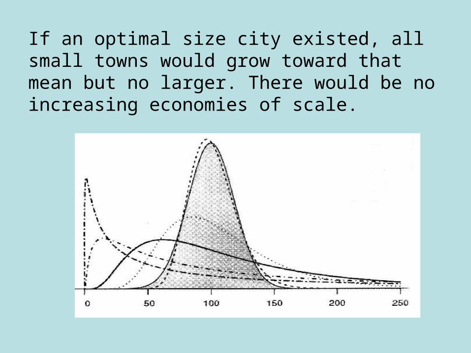
If an optimal size city existed, all small towns would grow toward that mean but no larger. There would be no increasing economies of scale.

However, there may be an optimal city-size distribution within “systems of cities”. Large systems tend toward a log-normal distribution with a few very large cities and many many small cities.

National population maps usually show this uneven distribution of city sizes
• “… differences in the kind and degree of benevolence of soil-climate-contour are capable of inducing differences in the density of the population throughout the entire territory, but only if all persons pursue the advantages inherent in their locations.” George Kinsley Zipf (p. 6, National Unity & Disunity: The Nation as a Bio-Social Organism; 1941)

George Kingsley Zipf(1902-1950)
• documented the skewed distribution of city sizes for many countries as a power law with an exponent very close to -1
• proposed that this skewed distribution resulted from a natural human process he called the “Principle of Least Effort”
• started a 50 year search by social scientists for an explanation for this very precise distribution which became known as “Zipf’s law”

Zipf’s Law
• Takes many forms
• K = r X P a
– K is the population of largest city– r is the rank (from the largest city)– P is the city population– a is a scaling factor ~ -1
• log K = log r – a log P

Linear (curving) and log-log (straight line) illustrations of Zipf’s power law
Power Law
y = 10x-1
R2 = 1
0.0
2.0
4.0
6.0
8.0
10.0
12.0
0 2 4 6 8 10 12
RANK
SIZ
E
Power Law
y = 10x-1
R2 = 1
1.0
10.0
1 10
RANK
SIZ
E
RANK SIZE
1 10.02 5.03 3.34 2.55 2.06 1.77 1.48 1.39 1.1
10 1.0

Using census data, Zipf showed the remarkably constant straight line log-log distributions of US city-sizes between 1790-1930

Many social scientists have tried to explain the precision of Zipf’s Law across space and over time. None have been entirely successful.
Paul Krugman:
“…we have to say that the rank-size rule is a major embarrassment for economic theory: one of the strongest statistical relationships we know, lacking any clear basis in theory.”
[p.44, Development, Geography, and Economic Theory, 1994]

Zipf dynamics:
• The rank-size rule is static but Zipf clearly recognized the dynamic nature of its underlying processes.
• Zipf stated: – “Specialization of enterprise, conditioned by the
various advantages offered by a non-homogeneous terrain, naturally presupposes an exchange of goods…”
– “with a mobile population, less productive districts will be abandoned for more productive districts”

Departures from the Zipf exponent of -1 (red curve on left graphs) indicate variations in city-size distributions and different urbanization processes.
Linear Distribution
y = 15.979x-0.8347
R2 = 0.6968
0
2
4
6
8
10
12
14
16
18
0 2 4 6 8 10 12
RANK
SIZE
Concave
y = 7.3543x-0.8419
R2 = 0.9941
1
10
1 10
RANK
SIZE

Departures from a Zipf exponent of -1
• Exponents between 0 and -1 (level slopes): even distributions of city sizes, relatively little urban diversity, characteristic of immature systems or perhaps managed efforts to promote inter-urban equity.
• Exponents greater than -1 (steep slope): diverse city-sizes, mature dynamic systems, large sample sizes.

List of U.S. Census data to illustrate Zipf’s law
• Incorporated towns (1790-2000)• Standard Metropolitan Statistical Areas
(1940-2000)• Minor Civil Divisions (1950-2000)• Urbanized Areas >50,000 & Urban Clusters
>2,500 (1960-2000)• Named Places (including unincorporated
locations)

Primary MSAs (major central cities)Concave distribution, Zipf exponent = -1.2

U.S. Urban Areas + Urban ClustersConcave distributionZipf exponent = -1.32

Distribution of named U.S. places for 1980
• 22500 Census recognized places (same as civil divisions for upper portion)
• Log-log distribution is linear in upper part, exponential in lower part

MCD Change 1980-90

Extent of Zipf’s Law
Zipf’s Law is useful for illustrating distribution of cities in the upper or fat tail of its log-normal distribution. Krugman suggests it applies only to U.S. cities of 200,000 people but we consider that it extends to smaller cities as well.
• Here is data for the US urban system from 1970 to 2000 based on populations of 22,500 ‘places’ which shows that the Law extends over at least 3 orders of magnitude
• Using just the upper (fat) tail, it is be seen that the distribution is remarkably stable between 1970 and 2000

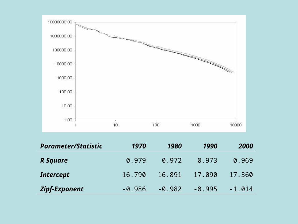
Parameter/Statistic 1970 1980 1990 2000
R Square 0.979 0.972 0.973 0.969
Intercept 16.790 16.891 17.090 17.360
Zipf-Exponent -0.986 -0.982 -0.995 -1.014

Zipf Dynamics Reworked: The US Urban System: 1790 to 2000
• We have taken the top 100 places from Gibson’s Census Bureau Statistics from 1790 to 1990 and added the 2000 city populations
• We performed log-log regressions to fit Zipf’s Law
• We then looked at the way cities enter and leave the top 100 giving a rudimentary picture of the dynamics of the urban system
• We may visualize these dynamics in many different ways

In this way, we have reworkedIn this way, we have reworkedZipf’s data (from 1790 to 1930) Zipf’s data (from 1790 to 1930)
3.5
4
4.5
5
5.5
6
6.5
7
0 0.5 1 1.5 2
Year r-squared exponent
1790 0.975 0.876
1800 0.968 0.869
1810 0.989 0.909
1820 0.983 0.904
1830 0.990 0.899
1840 0.991 0.894
1850 0.989 0.917
1860 0.994 0.990
1870 0.992 0.978
1880 0.992 0.983
1890 0.992 0.951
1900 0.994 0.946
1910 0.991 0.912
1920 0.995 0.908
1930 0.995 0.903
1940 0.994 0.907
1950 0.990 0.900
1960 0.985 0.838
1970 0.980 0.808
1980 0.986 0.769
1990 0.987 0.744
2000 0.988 0.737

0
10
20
30
40
50
60
1750 1800 1850 1900 1950 2000
Total Population in the Top 100 US Cities
Pop
ulat
ion
in M
illio
ns
Population NY City

1000
10000
100000
1000000
10000000
1 Log Rank 10 100
Chicago
Houston
Los Angeles
RichmondVA
NorfolkVA
Boston
Baltimore
Charleston
NewYorkCity
Philadelphia
Log CitySize

189019001910
1790 1800
1810
1820
1830
1840 Time
1850
1860
1870
18801920
1930
1940
1950
1960
1970
1980
1990
2000
Rank 1 20 40 60 80 100
Chicago
Houston
LA
RichmondVA
NorfolkVA
Boston Baltimore
Charleston

189019001910
1790 1800
1810
1820
1830
1840 Time
1850
1860
1870
18801920
1930
1940
1950
1960
1970
1980
1990
2000
(Log) Rank 1 10 100
Chicago
HoustonLA
Richmond VA
NorfolkVA
Boston Baltimore
Charleston
NY
Philly

Here we look Here we look at the half at the half lives of cities: lives of cities: the average the average number of number of years cities years cities remain in the remain in the list of largest list of largest 100 cities100 cities
Here is a plotHere is a plot
0
20
40
60
80
100
1780 1800 1820 1840 1860 1880 1900 1920 1940 1960 1980 2000

Applications of Zipf’s law to China
• China has the world’s largest urban population and one of the most dynamic of large urban systems.
• During the past half century, urban areas in China have undergone phenomenal changes that reflect both severe restrictions on large city growth and dramatically enforced decentralization policies.
• These Zipf calculations are, to some extent, constrained by limitations in data consistency and periodicity.

China census data
• Two categories of urban census data:• Provincial- and Prefecture-level cities (n = 234 in 1996);
• County-level cities (n = 400 in 1996).
Provincial- and Prefecture-level are highly urbanized and have a time-series since 1949. We used the total population living within the boundary of cities’ districts (shi qu) as the urban size.
• The total numbers of P&P cities:
1949: 56 cities; 1957: 60 cities; 1965: 63 cities;
1978: 95 cities; 1985:100 cities.
• Time series: 1949/1957/1965/1978/1985/1988/1992/1996.
• Starting with 1949, the largest 56 cities of each year were examined in rank-size space.
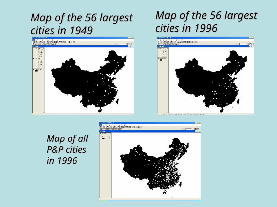
Map of Map of all P&P all P&P cities in cities in 19961996
Map of the 56 largest Map of the 56 largest cities in 1949cities in 1949
Map of the 56 largest Map of the 56 largest cities in 1996cities in 1996

Top 100 Chinese cities, 1949-1996
1
10
100
1000
1 10 100
rank
pop(
10,0
00 p
erso
ns)
1949 1957 1965 1978 1985 1988 1992 1996
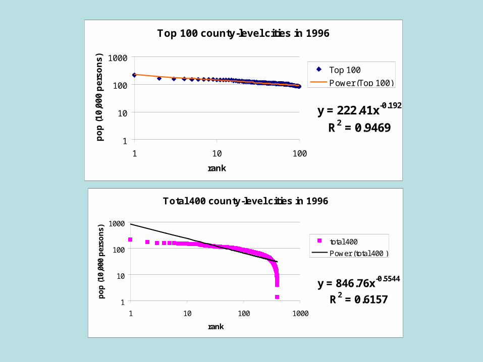
Top 100 county-level cities in 1996
y = 222.41x-0.192
R2 = 0.94691
10
100
1000
1 10 100
rank
po
p (
10
,00
0 p
ers
on
s)
Top 100
Power (Top 100)
Total 400 county-level cities in 1996
y = 846.76x-0.5544
R2 = 0.61571
10
100
1000
1 10 100 1000
rank
po
p (
10,0
00 p
erso
ns)
total 400
Power (total 400 )

Top 100 Cities based on urban district population, 1996
y = 1051.1x-0.5425
R2 = 0.9838
1
10
100
1000
10000
1 10 100
rank
pop
1996 urban district population
Power (1996 urban district population)

Top 56 cities in China, 1949-1996
Year 1949, y = 706.36x-1.0713
R2 = 0.9526
Year 1957, y = 1048x-0.9883
R2 = 0.9377
Year 1992, y = 896.64x-0.5252
R2 = 0.9857
Year 1996, y = 1035.1x-0.5385
R2 = 0.981
Year 1978, y = 825.72x-0.6493
R2 = 0.9726
Year 1965, y = 1321.2x-0.9619
R2 = 0.9385
Year 1985, y = 1016.6x-0.629
R2 = 0.9797
1
10
100
1000
10000
1 10 100
rank
pop(1
0,000
perso
ns)
1949
1957
1965
1978
1985
1988
1992
1996
Power (1949)
Power (1957)
Power (1992)
Power (1996)
Power (1978)
Power (1965)
Power (1985)

Zipf exponents for China’s 56 largest Prefecture and Provincial-level cities:
• Decreased from -1.02 in 1949 to a low of -0.52 in 1992 and then started to increase to -0.53 in 1996.
• Suggests the effects of stringent measures taken during the Maoist period, 1949-77, to limit urban migration, large city growth, and the concentration of coastal cities.
• Indicates independently functioning urban regions not well integrated into a single national system.

rank-time clock, absolute
0
10
30
50
60
70
80
90
1949
1957
1965
1978
1985
1988
1992
1996
ShanghaiNanjin
Suzhou
Guanzhou
Anshan
Wurumuqi
Thoughts about urban systems:
• Old assumptions– Cities emerge independently of other cities within
rural landscapes– Cities form vertical (Christaller) hierarchies– Big cities threaten environments
• New ideas– Cities have many horizontal links that build networks
and strengthen economies– Urban networks have unique stabilities and
vulnerabilities– Better human environments may result from a better
understanding of how “systems of cities” work

Questions for further research:
• How do urban systems organize themselves in space and time?
• What defines an “urban system” and what provides the basis for its stability and its vulnerabilities?
• What can we do to protect and enhance the quality of our urban systems and environments?