the dynamics of some epidemic models a thesis in
TRANSCRIPT

THE DYNAMICS OF SOME EPIDEMIC MODELS
by
KRISTIN JOY SUMPTER, B.A.
A THESIS
IN
MATHEMATICS
Submitted to the Graduate Faculty of Texas Tech University in
Partial Fulfillment of the Requirements for
the Degree of
MASTER OF SCIENCE
Approved
Accepted
Dean of the Graduate School
August, 1995
'^^ AFT 03
•^^^- ) ^ T ACKNOWLEDGMENTS
I would like to express my appreciation to the members of my committee,
Dr. Linda Allen, and Dr. Clyde Martin, for all their time and wisdom given to
me. I would especially like to thank Dr. Linda Allen for her extreme patience
and positive reinforcement during this project. Her enthusiasm motivated me to
continue and finish the work.
n
CONTENTS
ACKNOWLEDGMENTS ii
LIST OF FIGURES iv
CHAPTER
I. INTRODUCTION 1
II. VARIABLES AND MODEL PARAMETERS 3
III. SI AND SIR WITH NO VITAL DYNAMICS 6
IV. SI AND SIS MODELS WITH VITAL DYNAMICS 14
V. SIR AND SIRS MODELS WITH VITAL DYNAMICS 28
VI. SIS MODEL WITH GENERAL GROWTH DYNAMICS . . . . 42
VII. SUMMARY 49
REFERENCES 52
APPENDIX
A: LIAPUNOV STABILITY THEOREM 54
B: SI MODEL WITH NO VITAL DYNAMICS PROGRAM . . . . 56
C: SIR MODEL WITH NO VITAL DYNAMICS PROGRAM . . . 58
D: SIS MODEL WITH VITAL DYNAMICS PROGRAM 60
E: SIRS MODEL WITH VITAL DYNAMICS PROGRAM 62
F: SIR^R^S MODEL WITH VITAL DYNAMICS PROGRAM . . . 64
G: SIS MODEL WITH GENERAL GROWTH DYNAMICS PROGRAM 66
ni

LIST OF FIGURES
3.1 SI With No Vital Dynamics a = 0.5. The proportion of infectives approaches one, IQ/N = 0.7, So/N = 0.3 8
3.2 SI With No Vital Dynamics a = 5. The proportion of infectives approaches one, IQ/N = 0.7, SQ/N = 0.3 9
3.3 SIR With No Vital Dynamics a = 0.5. There is no epidemic IZo = 0.65, 7 - 0.5, lo/N = 0.3, So/N = 0.7, RQ/N = 0, Rn/N = , In/N = 12
3.4 SIR With No Vital Dynamics a = 5. There is an epidemic IZQ = 3.6, 7 = 0.5, lo/N = 0.3, So/N = 0.7, Ro/N = 0, Rn/N = ,
In/N= 13
4.1 Graphs of line y = x and curve y = g{x), IZ — a/{j-\-/3) = .9/.95 < 1. 18
4.2 Graphs of line y = x and curve y = g{x), IZ = a/(7 + /?) = 1.5/.5 > 1. X 0.520, XM ^ (^-706, X = g{c), where c = 0.920jX < Xm 19
4.3 Graphs of line y = x, and curve y = g{x), IZ = a/(7 + /?) = 5/.95 > 1. Xm ~ 0.309, X ? 0.490, Xm<x 20
4.4 Graphs of line y = x and curve y = g(x) when Xm <x 24
4.5 SIS With Vital Dynamics a = 0.4. The proportion of infectives approaches zero, IZ = 0.8, lim„^oo In/N = 0, j -\- /3 = 0.5, IQ/N = 0.7, 5o/A^ = 0.3 26
4.6 SIS With Vital Dynamics a = 5. The proportion of infectives approaches a positive limit, IZ = 10, lim„^oo In/N = 0.658, 7 +/? = 0.5, Jo/iV = 0.7,6'o/A^ = 0.3 27
5.1 SIRS With Vital Dynamics a = 0.5. The proportion of infectives approaches zero, 7Z = 0.83, lim^^oo In/N = 0 ,7 + /? = 0.6 31
5.2 SIRS With Vital Dynamics a = 5. The proportion of infectives approaches a positive limit, 7^ = 8, lim^^oo In/N = 0.45, 7 + /3 = .6. 32
5.3 SIR^R'^S With Vital Dynamics a = 0.5. The proportion of infectives approaches zero, IZ = 0.833, lim„^oo h/N = 0, 7 + /? = 0.6,^1 + /? = 0.6, 62 + 0 = 0.6, lo/N = 0.1, Rl/N = 0.25, Rl/N = 0.35, Rl/N = - . - . - . , Rl/N = ...., In/N = 35
IV
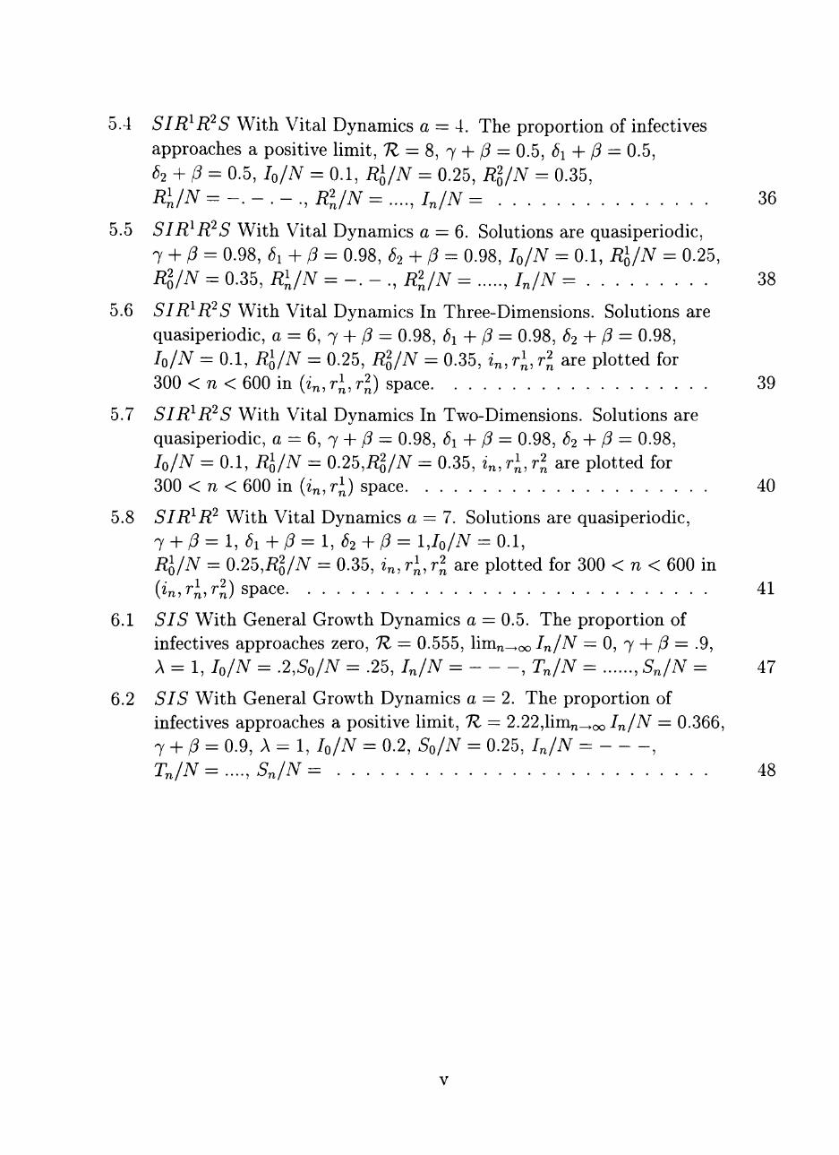
5.4 SIR^R'^S With Vital Dynamics a = 4. The proportion of infectives approaches a positive limit, 7^ = 8, 7 + /? = 0.5, Si-\- /3 = 0.5, ,52 + /? = 0.5, lo/N = 0.1, Rl/N = 0.25, Rl/N = 0.35, RijN = - . - . - . , Rl/N = ...., 4/A^ = 36
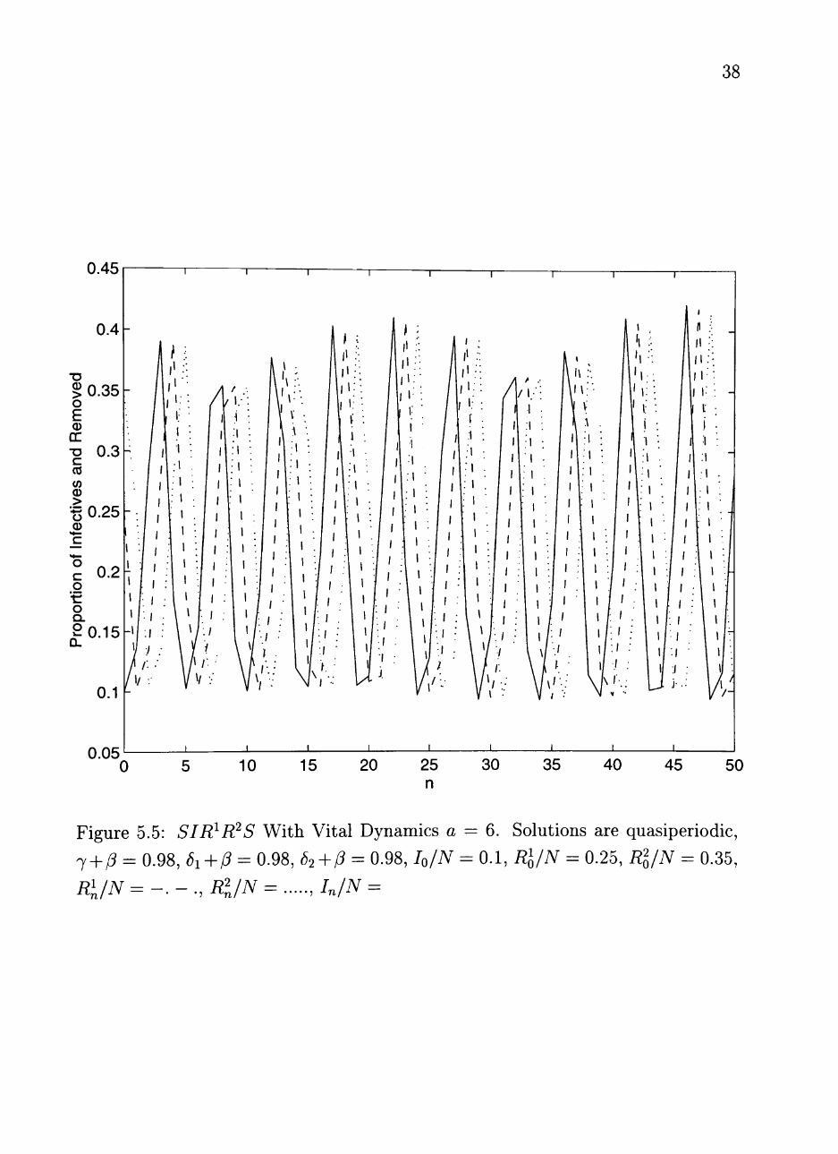
5.5 SIR^R^S With Vital Dynamics a = 6. Solutions are quasiperiodic, 7 + /? = 0.98, 1 + /? = 0.98, 62-^(3 = 0.98, /Q/TV = 0.1, Rl/N = 0.25, i?2/iV = 0.35, Ri/N = - . - . , i?2/7v = , IJN= 38
5.6 SIR^R^S With Vital Dynamics In Three-Dimensions. Solutions are quasiperiodic, a = 6, 7 + /? = 0.98, 61 + (5 = 0.98, 62-\-P = 0.98, lo/N = 0.1, i?J/iV = 0.25, Rl/N = 0.35, i„, r^, r^ are plotted for 300 < 72 < 600 in (in,rl,rl) space 39
5.7 SIR^R'^S With Vital Dynamics In Two-Dimensions. Solutions are quasiperiodic, a = 6, 7 + /? = 0.98, 61 + (3 = 0.98, 62-\-P = 0.98, /o/A^ = 0.1, Rl/N = 0.26,Rl/N = 0.35, z„, r^, r^ are plotted for 300 < 7i< 600 in (in^rl) space 40
5.8 SIR^R^ With Vital Dynamics a = 7. Solutions are quasiperiodic, j-^p=l^Si+p = l,S2-^P= IJo/N = 0.1, Rl/N = 0.25,Rl/N = 0.35, i„, r^, rl are plotted for 300 < n < 600 in (^n,^i,^n) space 41
6.1 SIS With General Growth Dynamics a = 0.5. The proportion of infectives approaches zero, IZ = 0.555, lim^^oo In/N = 0, 7 + /3 = .9, A = 1, V ^ ^ = •2,5o/A^ = .25, In/N = , Tn/N = , Sn/N = 47
6.2 SIS With General Growth Dynamics a = 2. The proportion of infectives approaches a positive limit, IZ = 2.22,lim„^oo In/N = 0.366, 7 -F /? = 0.9, A = 1, lo/N = 0.2, 5o/iV = 0.25, h/N = , Tn/N =...., Sn/N = 48

CHAPTER I
INTRODUCTION
We are observing the effects of a disease introduced into a population of suscep
tible individuals. It will be assumed that time is discrete; meaning the population
is observed every time interval. At. After introduction of an infection, individuals
are classified as either susceptible 5, infected / , or removed (immune) R. Thus,
a model is referred to as SIR if an individual is permanently immune to the dis
ease after having been infected and is referred to as SIRS if an individual has
only temporarily immunity and may become reinfected with the disease. An SIS
model implies an individual does not develop an immunity to the disease but is
immediately susceptible to the disease (after a time period At).
Kermack and McKendrick [13] were probably the first individuals to use the
SIR mathematical model to investigate the behavior of epidemics. Soper [20] was
one of the first to apply the model to an actual epidemic, a measles epidemic.
These initial investigations used the continuous-time version of the SIR model.
Discrete-time SIR and SIS models have also been used for modelling purposes.
Rvachev and Longini [19] simulated an influenza epidemic using a discrete-time
SIR model; Allen et al. [3] simulated a measles epidemic with a discrete-time
SIR model; Martin et al. [17] illustrated the dynamics of Chlamydia, a sexually-
transmitted disease, using a discrete-time SIS model.
The formulation of a discrete-time epidemic model may take different forms.
Allen [1] analyzed many of the basic SI, SIS, and SIR discrete-time models as
suming a particular form for the rate of contact. Because this rate of contact can
be shown to be an Euler discretization of the continuous-time formulation, the
models discussed by Allen [1] approximate the behavior of the continuous-time
formulation for small time intervals At. However, for large At, the discrete-time
models differ considerably from the continuous-time formulation. In this investi
gation, the contact rate for the discrete-time formulation is developed from first
principles and is based on the Poisson distribution. The contact rate formulation
used by Allen [1] is a linear approximation to the formulation considered here. The
analysis of the models considered in this investigation shows that their asymptotic
solution behavior is the same as that of their continuous analogues.
Some of the basic discrete-time models such as the SIR and SIS models that
use the same formulation considered here are discussed by Cooke [6], Hoppensteadt
[11] and Kocic and Ladas [16]. It is the purpose of this investigation to present
a complete discussion and analysis of the basic discrete-time models. The models
are then generalized to include vital dynamics, where births and deaths rates are
assumed to be equal. Finally, a generalized growth model is considered, where this
latter restriction on births and deaths is removed.
The presentation is divided into seven chapters. In Chapter II, the basic vari
ables and parameters are discussed. In Chapter HI, the basic SI and SIR models
with no vital dynamics-no births and deaths-are discussed. Then, in Chapter IV,
we discuss the SI and SIS models with vital dynamics-with births and deaths.
The SIR and SIRS models are presented in Chapter V and are generalized to
models with m removed classes. The SIS model is extended to a general growth
model in Chapter VI. A summary of the results is presented in Chapter MI. For
each of the models, numerical simulations are presented for illustration purposes.

CHAPTER II
VARIABLES AND MODEL PARAMETERS
In this chapter some common variables and parameters that will be used in
all the epidemic models presented will be discussed. The variable S will represent
the number of susceptible individuals, / will represent the number of infected
individuals, and R will represent the number of removed or immune individuals.
In addition, there are several parameters common to many of the models. The
number of individuals with whom an infectious individual will make sufficient
contact to pass the infection per unit time will be denoted by the parameter a > 0;
a is called the contact rate. We will assume that the population size remains
constant; number of births will equal number of deaths. The birth and death rate
will be symbolized by /?. The variable A'' will represent the total population size.
The probability of an individual recovering from the infection and returning to
the susceptible or immune class per unit time will be denoted by the parameter
7, 0 < 7 < 1. We will use 6 to symbolize the rate of loss of immunity from the
infection. Throughout the paper we will discuss a threshold value, which will be
defined in terms of the parameters. The threshold value is referred to as the basic
reproductive number and will be denoted by 1Z [9]. The basic reproductive number
represents the average number of secondary infections caused by one infectious
individual [4]. Thus, if 7^ > 1, an epidemic is sustained in the population, but
if 7^ < 1, the epidemic subsides and the population returns to the pre-infection
state.
The equations used in our models are difference equations and include an ex-

ponential term for the proportion not infected. This exponential form has been
assumed in other discrete-time epidemic models (see for example [3, 6]); it is based
on the Poisson distribution. The derivation of this exponential form depends on
the contact rate a, the average number of individuals with whom an infectious in
dividual will make sufficient contact to pass the infection per unit time. It follows
that alS/N is the average number of infections per unit time that are caused by
all of the infectives. The parameter /x = aIS/{SN) = al/N is the average number
of infections per susceptible individual per unit time. Now, the probability of k
successful encounters resulting in an infection of a susceptible individual by the
infective class per unit time is assumed to follow a Poisson distribution:
Thus, the probability that a susceptible individual does not become infective (no
successful encounters), is given by
p(0) = exp(-/i) = exp [-^Ij
The proportion of susceptibles that do not become infected per unit time is
denoted by: 5„+i = Sn exp(—;^/„), where Sn and /„ are the number of susceptibles
and infectives per unit time nAt and 5„+i is the number of susceptibles at time
(n + l)At. The proportion of susceptibles that do become infective (successful
encounters) is given by 1 - exp(—;^/n). Thus exponential contact expressions are
used in the models.
Another form for the proportion not infected has also been used in discrete-
time epidemic models (see for example, [1, 17, 19]). This model has the form

0
5„+i = 5„(1 - ^ ) in the simple susceptible equation which can be seen to be the
Unear approximation to the exponential, e x p ( - ^ ) « 1 - ain N f '^ ^ N

CHAPTER III
SI AND SIR WITH NO VITAL DYNAMICS
Two models are considered in this chapter, the SI and SIR models. No births
and deaths are included. The SI model is discussed first.
SI Model
In the SI model, the population is subdivided into two compartments, sus
ceptibles S and infectives / . The symbolism SI means that there is a transfer
from the susceptible to infective compartment; susceptibles become infective and
do not recover from the infection. Thus, the transfer continues until all individ
uals become infected. This type of model is very simple, but may represent the
dynamics of a very contagious disease during its early stages, e.g., common cold.
The continuous version of this model is discussed by Bailey [5]. The SI difference
equations have the following form:
Sn+l = 5 n e x p f - — / „ j
In+1 = Sn[l-exp(^-^In^^+In, (3.1)
where 5o, /o > 0 and Sn + In = N.
It is shown for model (3.1) that the total population size remains constant
and that eventually all individuals become infected. It can be easily seen that
Sn+i + In+1 = Sn + In and siucc So -\- lo = N, it follows that 5„ + /„ = N for
n = 0,1,. . . . The total population size is N for all time, n = 0,1, 2,.... The next
6

7
proposition shows that the entire population becomes infected, Hm„_oo h = N.
Proposition 1 In model (3.1), lim„^oo4 = A -
Proof. Note that {5„} is a monotonically decreasing sequence. Let ^oo = lim„_oo Sn^
Since lim„^oo4 = nm„^oo(A^ - Sn), then lim„^oo4 = oo exists. Since Soo < N
and /oo > 0, then I^ = (5oo - Sooexp{-fI^)) -\-1^ or since I^o > 0,S^ = 0.
Thus, lim^^oo In = N.
The conclusion states that the total number of infectives will approach the
population size. Also, the proportion of infectives, In/N approaches one. In the
following figures, the proportion of infectives is plotted against time. In Figure 3.1
the contact rate a = 0.5. In Figure 3.2 the contact rate is increased to a = 5. In
both cases the proportion of infectives approaches 1; the increase in the contact
rate allows the infectives to approach A at a faster rate.
SIR Model
In the SIR model, the population is subdivided into three compartments, sus
ceptibles S, infectives / , and removed or immune R. A continuous version of the
SIR model was first considered by Kermack and McKendrick ([13], [14], [15]) and
was applied by Soper [20] to a measles epidemic. An analysis for the discrete-time
SIR model, similar to the one given here, can be found in Hoppensteadt [11] and
Kocic and Ladas [16]. The model has the form:
Sn+l = Snexpl-—Inj
In+1 = 5„(l-exp(-^4))+/„(l-7)
Rn+1 = Rn + lln (3.2)

8
0.95-
0.85-
0.75-
0.65
Figure 3.1: SI With No Vital Dynamics a = 0.5. The proportion of infectives
approaches one, IQ/N = 0.7, So/N = 0.3.

0.95-
0.85-
0.75-
0.65
Figure 3.2: SI With No Vital Dynamics a = 5. The proportion of infectives
approaches one, lo/N = 0.7, SQ/N = 0.3.

10
where So Jo > 0,Ro > 0 and So + lo -\- Ro = N. It can be easily seen that
SnJn^Rn > 0 for Ti = 1,2,... and that 5„+i + 4+1 + Rn+i = Sn + In + Rn
for n = 0,1, Thus, Sn + h + Rn = N ioi n = 0,1,..., and the population
remains constant. Proposition 2 shows that as the epidemic dies out, the number
of infectives approaches zero.
Proposition 2 For model (3.2), lim„^oo4 = 0.
Proof-. Note that [Sn] is strictly decreasing and {Rn} is strictly increasing. Set
Soo = lim„^oo Sn and R^o = lim^^oo^n- Then Soo > 0 and Roo > 0. By taking
limits in the third equation in model (3.2) lim^^oo In = 0; the total number of
infectives approaches zero.
In Figures 3.3 and 3.4, the proportion of infectives, In/N, is plotted against
time: the proportion of infectives approaches zero. The proportion of removed
individuals, Rn/N, also approaches a limit. Figure 3.3 verifies Proposition 2 when
the contact rate a = 0.5. In Figure 3.4, the contact rate is increased to a = 5.
In this SIR model, the number of infectives either increases or decreases ini
tially before approaching zero. If the number of infectives increases initially be
fore approaching zero, meaning if /i > /Q, then we say that there is an epi
demic. Using the /„+! equation of model (3.2) it can be shown that /i > IQ,
h = Soil - e x p ( - f Jo)) -H /o(l - 7) > 4 , if
5 o [ l - e x p ( - f / o ) ] > 1,
lol
The expression on the left is referred to as the effective reproductive rate [4], we
shall denote it as 7 o• If ^o = (5'o(l - e x p ( - f / o ) ) / 4 7 > 1, then an epidemic

11
occurs. In Figure 3.3, 1Zo = 0.65 < 1; an epidemic does not occur. In Figure 3.4,
7 0 = 3.6 > 1; and an epidemic does occur. This result is reasonable since the
contact rate was increased considerably, the disease is spread rapidly with more
contacts; more individuals contract the disease initially.

12
\J.I
0.6
• D 0) > | 0 . 5 0) CC • Q
c > - 4 0) >
^ ^ o o ^ ^ •^0 .3 '1
o c o •c
§.0.2 o _ CL
0.1
/ /
/ 1
- 1 1
1 1
1 1 1 1 1 1 1
, — •
...-^ - y^
y
/ •
/ /
/ /
/
/ /
/ /
/ /
/
1 1 1 1 r — — 1 1
1 1
-
-
-
-
-
1 1
0 8 10 12 14 16 18 20 n
Figure 3.3: SIR With No Vital Dynamics a = 0.5. There is no epidemic T o = 0.65,
^ = 0.5, h/N = 0.3, So/N = 0.7, Ro/N = 0, Rn/N = , In/N =

13
/
10 n
12 14 16 18 20
Figure 3.4: SIR With No Vital Dynamics a = 5. There is an epidemic TZQ = 3.6,
7 = 0.5, lo/N = 0.3, So/N = 0.7, Ro/N = 0, Rn/N = , In/N =

CHAPTER IV
SI AND SIS MODELS WITH VITAL DYNAMICS
In this chapter, SI and SIS models are considered. Births and deaths are in
cluded and the birth rates equal the death rates (0 < /? < 1) so that the population
size remains constant. Both models can be described by one system of difference
equations. In the SI model, individuals do not recover from infection, but remain
infected. However, in the SIS model, individuals recover from infection with prob
ability 7. It is assumed that 0 < 7 < 1 and 0 < / ? H - 7 < l ; i f 7 > 0 the following
system is an SIS model and if 7 = 0, the system is an SI model. The SI and
SIS model with vital dynamics has the following form:
Sn+l = Sn exp f - yy^j + (7 + ^)In
In+1 = 5„ ( 1 - e x p ( - ^ / „ ) ) + 4 ( 1 - 7 - / ? ) (4.1)
where So, lo > 0 and 5o + /o > N. It can easily be seen that 5n -I- /„ = A" for all n.
Model (4.1) is a generalization of a discrete SIS model considered by Cooke
et al. [6]. In the model of Cooke et al. [6], it was assumed that 7 = 1 and
/? = 0; no births or deaths were included and At was assumed to be the period
of infectivity, infected individuals moved to the susceptible class after one period.
Cooke et al. [6] proved that if a < 1, then the number of infectives approach zero,
but if a > 1, solutions approach a positive steady-state, an endemic equilibrium.
The parameter a in their model represents the basic reproductive number 7Z but
for our model (4.1), the basic reproductive number is given by 7^ = 0/(7 + (3),
0 < ^-f ^ < 1. Note that if 7-h/? = 0, then model (4.1) simplifies to the SI model
14

15
considered in Chapter III. The following theorem uses the approach of Cooke et
al. [6] to generahze the results to model (4.1).
Theorem 1 ; If IZ = 0/(7 + P) < 1, then the solutions to model (4.I) satisfy
lim„_oo4 = 0. If1Z>l, then solutions to model (4.I) satisfy lim„^oo4 = I*,
where /* is the unique positive solution to
A ^ - ( l + 7 + /?)/*
' - - . • • ) •
Before we proceed with the proof of the theorem, the difference equations in
model (4.1) are simphfied by considering proportions. Let x\ = In/N and xl =
Sn/N. Model (4.1) becomes
^l+i = ^nexp(-aa:i) + (7 + ^)a;i
n+i = ^ n ( l - e x p ( - a x i ) ) + j ; i ( l - 7 - / ? ) . •^n
If we let x\ = Xn and use the fact that x^ = 1 - x„, we only need to consider
the equation for the proportion of infectives, x„:
Xn+i = (1 - Xn)[l - exp(-aa:„)] -f (1 - 7 + (5)xn. (4.2)
The proof of the theorem is now given.
Proof The proof proceeds in several parts. First it is easily seen that solutions to
(4.2) are nonnegative and bounded by one.

16
If 0 < x„ < 1, then 0 < 1 - exp(-ax„) < 1 and from (4.2)
Xn+l < {I ~ Xn){l) -\-Xn{l) = 1.
Also,
Xn+l > (1 - Xn){0) -f {0)Xn = 0.
Thus, 0 < Xn+i < 1 given 0 < i;„ < 1.
Let Xn+i = g{xn), where g{x) = (1 - x){l - exp{-ax)) + (1 - 7 - /3)x. Then
it will be shown that ^'(0) = a-\-1 - P - ^ and g"{x) < 0 for 0 < a: < 1.
g'{x) = (1 - x)[aexp(-ax)] - [1 - exp(-ax)] - (1 - 7 - /?);
thus, ^'(0) = a + l - 7 - / ? . Also,
g"{x) = —(1 — x)(a^exp(—ax)) — (2aexp(-ax)) < 0
for 0 < X < 1.
Next the first part of Theorem 1 is proved. If IZ = a/(y -\- (3) < 1, then
lim„^oo In = 0. Note that x = 0 is a fixed point or steady state of g:
X = 1 — exp(—ax) — x-\- xexp(—ax) 4- x — 7^ = g{x)
If ^ = 0, then g{x) = 0 so x = 0 is a steady state.
We need to show that this steady state is the only steady state. We showed
g"{x) < 0 for 0 < X < 1 so Jo g"{s)ds < 0 for 0 < a: < 1.
Now, J^ g"{s)ds = g'{x) - g'{0) < 0, so g'{x) < g'{0) = a + 1 - 7 - /3, so
g'{x) <a-\-l-j- (3<1.

17
Thus, g'{x) - 1 < 0 for 0 < X < 1 or
(g'(s) - l)ds = [g{x) -x]- lg{0) - 0] < 0 J (J
or g(x) - x < 0. Thus, g{x) < x. The curve g{x) is below the line y = x and
X = 0 is the only steady state. Now we need to show that Xn+i = g{xn) generates
a sequence x„ such that Hm^^oo a:„ = 0. We know 0 < g(x) < x for 0 < x < 1 and
^(0) = 0. (See Figure 4.1.)
^1 = g{xo) < xo
X2 = g{xi) < Xl .
In general,
Xn+i — gy^n) *^ ^n-
Thus we have a monotonic decreasing sequence:
Xo > Xl > X2 > > Xn> Xn+l > > 0
A monotonic sequence converges if and only if it is bounded [18]. Thus, all that
is left to show is lim^^oo Xn = 0. We know lim„^oo ^n = x. But lim„_^oo n =
lim„_^oo n+i = lim„^oo gi^n) = g(x) so X = ^(x). But the only x where x = ^(x)
is X = 0 since x is the only steady state. Thus lini„_oo3:n = 0, if 7^ < 1. (See
Figure 4.1.)
The next part of the proof is to show that if 7^ > 1 then lim„^oo x ^ = x*, where
0 < X* < 1. Note that ^(0) = 0, ^(1) = 1 - 7 - /? < 1, g'{0) = a - h l - 7 - / ? > l ,
^'(1) = exp(—a) — 7 — /? < 1, so there is at least one point of intersection between
y = X and y = ^(x) for 0 < x < 1 because g is continuous. (See Figures 4.2 and
4.3.)

18
>'0.5-
Figure 4.1: Graphs of line y = x and curve y = ^(x), TZ = 0/(7 -!-/?) = .9/.95 < 1.
/ "

19
Figure 4.2: Graphs of line y = x and curve y = g{x), TZ = a/{j + /?) = 1.5/.5 > 1.
X ^ 0.520, XM « 0.706, x = g{c), where c = 0.920, x < x^.
20
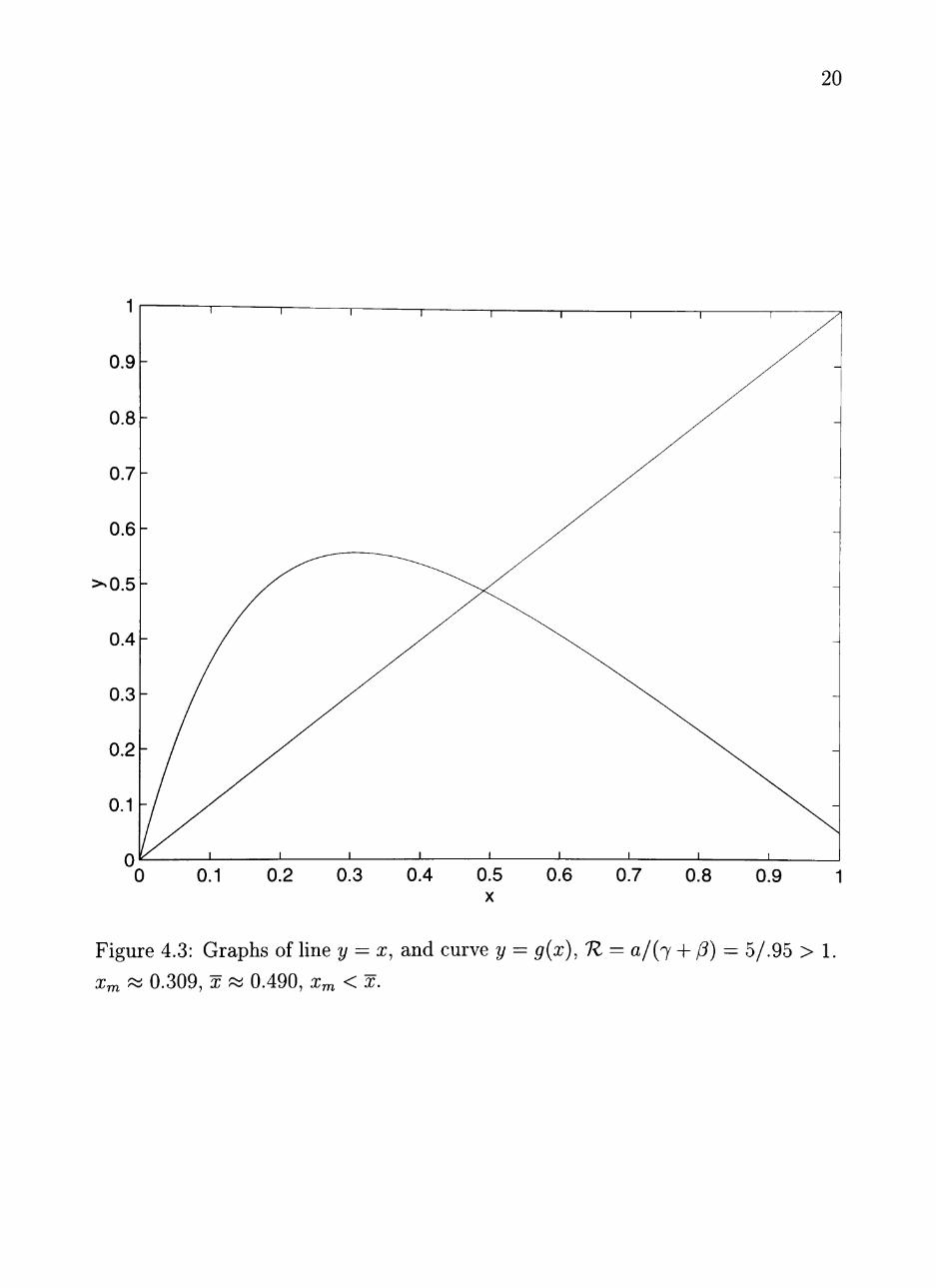
Figure 4.3: Graphs of line y = x, and curve y = ^(x), 1Z = a/{^ + (3) = 5/.95 > 1.
Xm ~ 0.309, X 0.490, x^ < x.
21
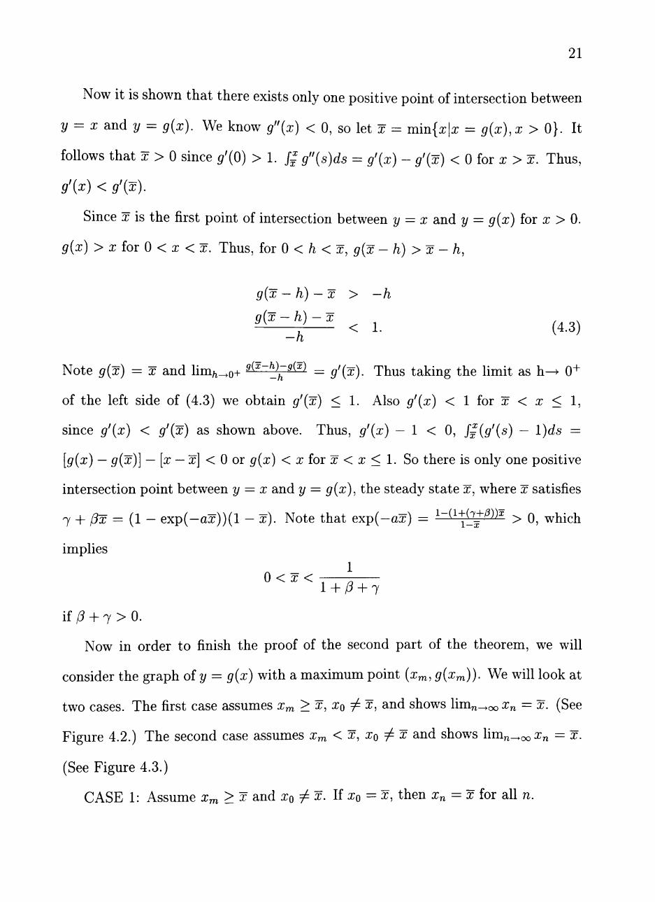
Now it is shown that there exists only one positive point of intersection between
y = X andy = g{x). We know g"{x) < 0, so let x = min{x|x = ^(x),x > 0}. It
follows that X > 0 since ^'(0) > 1. / | g"{s)ds = ^'(x) - g'{x) < 0 for x > x. Thus,
g'{x) < g'{x).
Since x is the first point of intersection between y = x and y = g{x) ior x > 0.
g{x) > X for 0 < X < X. Thus, for 0 < / i< x, ^(x - /i) > x - h,
g(x - h) -X > -h
gCx — h) — X , , r < 1- (4-3)
—h
Note g{x) = x and Hm/, o+ ^ ~ )~ ^ ) = ^'(x). Thus taking the Umit as h ^ 0+
of the left side of (4.3) we obtain g'{x) < 1. Also ^'(x) < 1 for x < x < 1,
since ^'(x) < ^'(x) as shown above. Thus, ^'(x) — 1 < 0, f^(g'{s) — l)ds =
[^(x) — ^(x)] — [x — x] < 0 or ^(x) < X for X < X < 1. So there is only one positive
intersection point between y = x and y = ^'(x), the steady state x, where x satisfies
7 + /?x = (1 - exp(-flx))(l - x). Note that exp(-ax) = ^-i^+ij+^))^ > o, which
implies 1
0 < X < 1 + /3-F7
if /? + 7 > 0.
Now in order to finish the proof of the second part of the theorem, we will
consider the graph ofy = g{x) with a maximum point (x^, ^(x^)). We will look at
two cases. The first case assumes x^ >X,XQ^ X, and shows lim^^oo ^n = oc. (See
Figure 4.2.) The second case assumes x^ < ^, ^o / ^ and shows lim^^oo ^n = x.
(See Figure 4.3.)
CASE 1: Assume x^ > x and XQ ^ x. If XQ = x, then x„ = x for all n.

22
Case la. 0 < XQ < x < x^.
In this case, x > ^(x) > x for 0 < x < x. Thus Xi = ^(XQ) > XQ, X2 = ^(xi) >
Xl. In general, XQ < Xi < X2 < ... < x„ < x^. The sequence, x„ is monotonic
increasing and bounded by x^; it converges. Also since ^(x) has only one positive
point of intersection with the fine y = x (one fixed point) and that intersection is
X, the sequence x„ approaches x.
Case lb. X < Xo < c where g{c) = x.
In this case, Xi = ^(xo) < Xo < x^, X2 = ^(xi) < xi < x^. The sequence Xn is
a monotonic decreasing sequence bounded by x^. The sequence Xn tends to the
steady state x.
Case Ic. x^ < c < Xo where g{c) = x.
In this case, xi < x < xo, but then Xi < X2 < ... < x„ < ... < x. The sequence,
Xn, is bounded by x and monotonically increasing to x.
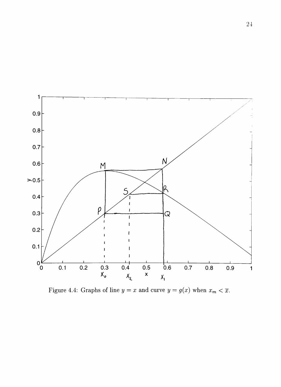
CASE 2: Assume x^ < x.
v^ase za. xo -— Xj .
Let M = g{xm) and draw MN horizontally to point N on the line y = x.
(See Figure 4.4.) Draw N to the x-axis. This point is Xi = g{xm) = M. Draw
a perpendicular line from M onto the x-axis meeting line y = x at F. Draw PQ
parallel to MN. Since PN Ues on y = x line, it has slope 1 and MQ then has slope
-1 . Thus QPMN is a square. Now,
^'(x) = exp(-ax)[l -h a(l - x)] - 7 - /? > exp(-ax) --f - P >-J - P >-1,
so g'{x) > - 1 for 0 < X < 1.
The curve y = g{x) must He above the diagonal MQ for X;„ < x < Xi and NQ
intersects the curve at point R above Q. A horizontal line through R intersects

23
y = X at point S above and to the right of P. Thus,
Xm<X2 = g(xi) = g{g{xm)) < Xl
Xl > X3 = ^(x2) = ^(^(xi)) = g{g(g{xm))) > X2.
It follows from Figure 4.4, that
Xo = Xm < X2 < < X3 < Xl .
Even numbered iterates must converge to x' and odd numbered iterates must
converge to x".
Suppose x' / x". Without loss of generality suppose x' < x". Then x' and x"
must be two periodic points of iteration, meaning fixed points of g{g{x)). Consider
the sequence starting from x'. Drawing a square with one corner at (x', g{x')) and
following the same argument as above g{g{x')) > x'. This contradicts the fact that
we assumed x' and x" were fixed points of g{g{x)) so x' and x" must not be two
periodic points of iteration. Thus, it must be the case that x' = x" or x' = x. The
sequence starting with xo = Xm converges to x, since x is the only fixed point of g.
Case 2b. x < xo < 1.
Then,
Xl = g{xo) < X.
The remaining cases take care of the proof of this case.
Case 2c. x^ < XQ < ^
An argument similar to case 2a shows x^ < X2 < X4 < < X5 < X3 < xi and
that the sequence x„ converges to x since the sequence falls inside [x^, c/(x^)].
Case 2d. 0 < Xo < Xm
24
0.3 0.4 0.5 X
0.7 0.8 0.9
Figure 4.4: Graphs of line y = x and curve y = ^'(x) when Xm < x.

25
After a finite number of iterations we get to a point Xn such that Xm < Xn <
g(xm) < X. The sequence x„ converges to x as in case 2c. This concludes the proof
of the theorem.
The theorem is illustrated with some examples. In Figure 4.5, we let a = 0.4
and 7 -h /? = 0.5, then 7^ = 0.8 < 1 and the proportion of infectives approaches
zero. In Figure 4.6, the contact rate was increased to a = 5, then 7^ = 10 > 1.
We expect the proportion of infectives to approach a positive limit; in this case
X = 0.657.

26
Figure 4.5: SIS With Vital Dynamics a = 0.4. The proportion of infectives
approaches zero, U = 0.8, lim„^oo In/N = 0, 7 + / = 0.5, h/N = 0.7, 5o/A^ = 0.3.

27
0.69
0.68-
0.67-
0.66-
0.65-
0.64
Figure 4.6: SIS With Vital Dynamics a = 5. The proportion of infectives
approaches a positive limit, IZ = 10, limn^oo In/N = 0.658, 7 -h /? = 0.5,
/o/iV = 0.7,5o/A^ = 0.3.

CHAPTER V
SIR AND SIRS MODELS WITH VITAL DYNAMICS
In this chapter we analyze SIR and SIRS models with vital dynamics. In
the SIR model of Chapter III, births and deaths are included (P > 0). We also
allow temporary immunity, individuals lose immunity with probability 6 >0 and
return to the susceptible class, an SIRS model. The difference equations for these
models have the following form:
Sn+l = Snexp(^-^In^-\-Rn{S-\-p)-\-PIn
In+1 = Sn[l-exp(^-^In^^+In{l-J-p)
Rn+1 = Rn{l-S-P)+Jln (5.1)
where 5o-l-/o + ^o = N, So, /o > 0 and RQ > 0. Note that the total population size
remains constant, Sn + In + Rn = N, and solutions are nonnegative. If ^ = 0 and
/? = 0, then system (5.1) simplifies to the SIR model for Chapter III. It is assumed
that 0 < 7 4- /? < 1 (as in Chapter IV) and 0 < (5 + /? < 1. It is proved for 71 < 1
that solutions approach a disease-free state. Cooke et al. [6] proved a similar
result in the case that a < 1. (Our proof uses the method employed by Cooke et
al. [6]). We have been unable to show that the reverse inequality, 7^ > 1, impHes
solutions approach an endemic equilibrium but numerical simulations indicate that
this result may be true.
In the following analysis, the normahzed system is considered. Let i„ = In/N.
28
29
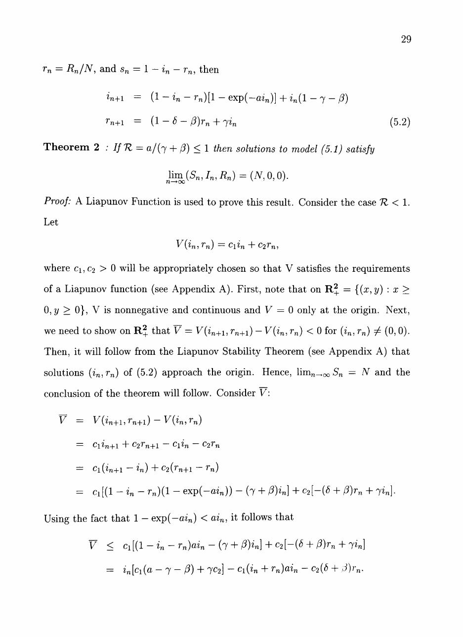
Tn = Rn/N, and s„ = 1 - ?„ - r„, then
in+1 = ( l - « n - r - n ) [ l - e x p ( - a z „ ) ] + i „ ( l - 7 - / ? )
Tn+l = {I - S - P)rn -\-Jin ( 5 .2 )
Theorem 2 : Ifn = a/{j + 0) < 1 then solutions to model (5.1) satisfy
YimJ^Sn, In, Rn) = {N, 0,0).
Proof: A Liapunov Function is used to prove this result. Consider the case 7^ < 1.
Let
V{in,rn) = Clin -\-C2rn,
where Ci, C2 > 0 will be appropriately chosen so that V satisfies the requirements
of a Liapunov function (see Appendix A). First, note that on R J = {{x,y) : X >
0,2/ ^ 0}, V is nonnegative and continuous and V = 0 only at the origin. Next,
we need to show on R j that V = V{in+i,rn+i) — V(in, rn) < 0 for [in, rn) / (0, 0).
Then, it will follow from the Liapunov Stability Theorem (see Appendix A) that
solutions {in,fn) of (5.2) approach the origin. Hence, lim^^oo-S'n = N and the
conclusion of the theorem will follow. Consider V:
V = V{in+i,rn+i) - V{in, rn)
= CiZ„+i + C2rn+i - Clin - C2r„
= Ci{in+1 - in) + C2{rn+1 " Tn)
= ci[(l -in- rn){l - exp(-mn)) - (7 + ^)^n] + C2l-{S -f- P)rn -h Jin].
Using the fact that 1 - exp(-az„) < ain, it follows that
V < Ci[{l-in-rn)ain-{j-^(^)in]^C2[-(S^P)rn-\-jin]
= in[ci{a - J - P)-\- 7C2] - Ci{in 4- rn)ain - C2(S + ,d)r„.

30
For V to be negative we need to choose Ci and C2 such that Ci (a - 7 -/?) 4-7C2 < 0.
Since 1Z < l,a < (P + j), then positive numbers Ci and C2 can be chosen such that
ci ^ 7
C2 J + P - a
Then V < 0 for all points in R^ except for the origin. The Liapunov function
V satisfies the requirements of the Liapunov StabiUty Theorem, solutions of (5.2)
approach the origin if 7^ < 1.
In the case that 7^ = 1, by choosing C2 = 0, the same analysis shows that
in approaches zero. However, from system (5.2) it can easily be seen that if
lim„^oo in = 0, then linin^^oo n = 0. Hence, the theorem holds for 7^ = 1.
The results of Theorem 2 are illustrated numerically. In Figure 5.1 the contact
rate is a = 0.5, 7 -I- /? = 0.6 and IZ = 0.83 < 1. In this case, the proportion
of infectives approaches zero. In Figure 5.2, the contact rate was increased to 5,
then 7^ = 8 > 1; the proportion of infectives approaches a positive limit. This
latter result was true for all of the simulations where 7^ > 1; a positive endemic
equilibrium was approached.
The SIRS model with vital dynamics is extended to a model that includes m
removed classes, m > 2. The system of difference equations has the form:
Sn+l = Snexp{-^In)^SmR';: + P{In + R'n + .... + R'::)
In+1 = 5 n ( l - e x p ( - ^ J „ ) ) + / n ( l - 7 - / ? )
K+1 = Rl{l-ei-P)+jIn
R^^^ = R^{l-em-P) + ^n.-lRn (5-3)
where So + h + ^tiR^ = ^^ ^oJo > 0 and R^ > 0, i = 1 ,m. Also it is

31
0.25 -
0 .15-
0.05-
Figure 5.1: SIRS With Vital Dynamics a = 0.5. The proportion of infectives
approaches zero, 7^ = 0.83, lim„_oo In/N = 0, j + P = 0.6.

32
0.65-
0.55-
0.45-
0.35
Figure 5.2: SIRS With Vital Dynamics a = 5. The proportion of infectives
approaches a positive limit, 7^ = 8, lim„_oo In/N = 0.45, j - \ - p = .Q.

33
assumed that 0 < j - \ - p < 1 and 0 < Si-{- P < I, i = 1, , m. For this model, as
in previous models, it is easily proved that solutions are nonnegative and satisfy
Sn + In + ^T=lRn = N.
The next theorem proves that lilZ = a/{j -\- p) < 1, then the system becomes
disease-free. Unlike model (5.2) with only one removed class, solutions to model
(5.3) do not approach a positive endemic equilibrium for all parameter values
satisfying IZ > I. It is shown numerically that when IZ is sufficiently large that
solutions exhibit periodic and quasiperiodic behavior.
Cooke et al. [6] considered the special case j-\-P = 1 and ^^4-/3 = 1,2 = 1, m.
For their special case, they proved if a < 1, then lim^^oo In = 0.
The analysis in the following theorem is similar to Theorem 2; the normalized
system is used in the proof, where in = In/N,r\^ = R\/N,i = l,....,m, and
^n ~ ^ '"n ^i=l'n-
Theorem 3 : If IZ = a/{j -\- P) < I, then solutions to model (5.3) satisfy
lim(5„,4,i?i,....C) = W0,0, ,0) n—>oo
Proof: The following Liapunov Function is appHed in this case:
V{in, rl , C ) = Clin 4- C2ri + -h c^+iC,
where the constants Ci > 0 will be suitably chosen. Note that V is nonnegative in
Ry+^ and is only zero at the origin.
Suppose IZ<i, then it will be shown that F < 0 for some positive c .
V = F ( w i , d , - - . C + i )
= ci{in+i - in) + C2{rl^+i - rl) 4-... -\- Cm+i(C+i " C )

34
= ci[{l - in - rl^-
... - C ) ( l - exp(-ai„)) - (7 4- P)in] -h C2[7«n - ( 1 + P)r'n]
•••+C^+l[(^m-lC"'-( '5m+/?)Cl-
Since 1 — exp(—ai„) < ain,
V < Ci[{l-in-rl,-...-r^)ain-{j^P)in]-C2[rl^i6i+P)-jin]-
...-Cm+lK{Sm+P)-6m-ir:^-']
< in[ci{a -j-P)-\- C27] - r-i[c2(^i 4- /?) - C361] - rj[c3(^2 4- /?) - c^62] -
••• - C~MCm(<5m-l + P) - Cm+l^m-l] " Ciain{in + ^^ 4"
. . .4-C)-Cm+lC('5m + /3).
Thus V will be negative if the Q are chosen such that
Ci 7 , — > a n d C2 > C3 > C4 > ... > Cm+i > 0.
C2 J -\- P - a
It follows from the Liapunov Stability Theorem (see Appendix A) that if 7^ < 1,
solutions {in,rl,rl, ...,r^) to model (5.3) will aproach zero. If 7^ < 1, the result
of the theorem follows; system (5.3) becomes disease-free.
If 7^ = 1, y < 0 if Ci = 0 for i = 2,..., m and Ci > 0. In this case, lim„_oo in = 0,
but from system (5.3) it easily follows that liuin^ooirl, rl, ...,r^) = (0,0, ...,0).
The theorem is proven.
Figure 5.3 illustrates Theorem 3 for the case m = 2. In Figure 5.3, we let the
contact rate be a = 0.5, j-\-P = 0.6,6i-^P = 0.6,62^P = 0.6, and IZ = 0.833; the
proportion of infectives approaches zero. In Figure 5.4, we changed the contact
rate to a = 4, 7 + /? = 0.5, Si + P = 0.5, 62-^ P = 0.5 and 7^ = 8; the proportion
of infectives approaches a positive Hmit.

35
0.35
0.3-
• o o ^0.25 o
CC -a c (C w CD >
0.2
1
" \ \ \
- \ \ \ \ \
1
-
-
10 15 n
Figure 5.3: SIR^R'^S With Vital Dynamics a = 0.5. The proportion of infectives approaches zero, 1Z = 0.833, \imn^ocIn/N = 0, j + P = 0.6,6i -^ P = 0.6, 62-hP = 0.6, lo/N = 0.1, Rl/N = 0.25, Rl/N = 0.35, R'JN = - . - . - . .
Rl/N =...., In/N =

36
•o > o E (D
CC C CC (O CD _> '•4—'
o CD
O c g o Q. O
u.oo
0.3
0.25
0.2
0.15
1
/
'J 1 Y / A/
y \ \ A- •
\ \ V ^ \ "
1
1
1
^ ^ ^ __
1 1
_
_
-
0 10 15 20 25 n
Figure 5.4: SIR^R'^S With Vital Dynamics a = 4. The proportion of infectives approaches a positive limit, IZ = S, j -\- P = 0.5, 6i -{- p = 0.5, 62 -\- P = 0.5. lo/N = 0.1, Rl/N = 0.25, Rl/N = 0.35, R'JN = - . - . - . , Rl/N = ...., In/N =

37
System (5.3) has a much wider array of behavior than previous models as can
be seen in the following figures. In Figure 5.5, we increased the contact rate to
a = 6, 7 -h /? = 0.98, 6i + P = 0.98, and 62 + P = 0.98. The solutions appear to
be quasiperiodic. The solutions may not have a rational period. This behavior
is more apparent in Figures 5.6 and 5.7 where the behavior for in,Tn, and r„ is
plotted for 0 < n < 300 in {in, r^, rl) space. This same figure is projected into the
in. rl plane in Figure 5.7. Figure 5.8 shows that for a = 7, 7 4- /? = 1, 1 4- /? = 1,
and 62 -\- P = i there appears to be a periodic solution of period 5. Solutions in
Figure 5.8 are plotted in {in,rl,rl) space for 300 < n < 600.
38
0.45
Figure 5.5: SIR^R^S With Vital Dynamics a j + p = 0.98, di^P = 0.98, 62^P = 0.98, h/N
Ri/N =-.-., Rl/N = ,In/N =
- 6. Solutions are quasiperiodic, 0.1, Rl/N = 0.25, Rl/N = 0.35,

39
rl 0 0
Figure 5.6: SIR^R'^S With Vital Dynamics In Three-Dimensions. Solutions are
quasiperiodic, a = 6, j - \ - P = 0.98, Si + P = 0.98, S2 + P = 0.98, h/N = 0.1,
Rl/N = 0.25, Rl/N = 0.35, in, r^ rl are plotted for 300 < n < 600 in (z„, r^ rl)
space.

40
0.45
0.4
0.35
0.3
0.25
0.2
0.15
0.1
0.05
^+|.^+t-^+H-w-^+^ -^ -Hf-
-Hf %
\ \
\ %
%
\
#
^ ^ 4 ^ - H f 4 t t f 4 ^ ^ -0- -0 -K4- -^
-tt*-^^
0.05 0.1 0.15 0.2 0.25 r l
0.3 0.35 0.4 0.45
Figure 5.7: SIR^R^S With Vital Dynamics In Two-Dimensions. Solutions are
quasiperiodic, a = 6, j - ^ P = 0.98, Si + P = 0.98, S2-\-P = 0.98, h/N = 0.1,
Rl/N = 0.25,Rl/N = 0.35, in,r'i,r2 are plotted for 300 < n < 600 in {in,rl)
space.

41
rl 0 0
Figure 5.8: SIR^R'^ With Vital Dynamics a = 7. Solutions are quasiperiodic, .y^(3 = lj^+P = i^S2 + P=hh/N = 0.i,Rl/N = 0.25,Rl/N = 0.35,in,rlrl
are plotted for 300 < n < 600 in {in, r^ rl) space.
CHAPTER VI
SIS MODEL WITH GENERAL GROWTH DYNAMICS
The final model that is considered is an SIS model with general growth dynam
ics. In this model, the total population size is not restricted so that 5„ + /„ = A ,
but Sn + In = Tn, whcrc Tn represents the total population size. It is assumed that
Tn satisfies logistic growth with carrying capacity A , that is,
_{_X + l)NTn
' " + 1 - N + XTn '
where A > 0 and 0 < To < A . The SIS model has the form:
Sn+l = 5 . ( / ( 5 „ + 4 ) - h e x p ( - ^ / „ ) ) + ( 7 4-/?)4
In+1 = Inf{Sn-^In)-^Sn{l-exp(^-^In^^+In{l-J-p) (6.1)
where So, h>0,So-\-h< N and / (5„ -H h) = f{Tn) = A(A - Tn)/{N 4- ATJ.
The SIS model with general growth dynamics behaves similar to the SIS model
discussed in Chapter IV. The following proposition shows that the total population
size approaches the carrying capacity monotonically. It will follow from Proposition
3 that solutions to (6.1) are positive and satisfy 0 < Sn+h < N. Then applying the
proposition, it can be shown that in certain cases the SIS model (6.1) approaches
a disease-free state if 7^ < 1 and a positive endemic state if 7^ > 1.
Proposition 1 The total population size T„ = 5n 4- h satisfies Tn < Tn+i for
72 = 0,1,2, and limn_ oo Tn = N.
Proof It follows directly from the difference equations (6.1) that
Tn+l = Tn{f{Tn) ^ I) = ^^^^^^^J" • (6-2)
42

43
Equation (6.2) has two steady-states, T = 0, and T = A . The right-hand side
of equation (6.2), y = x{f{x) 4- 1), is increasing for xeK+. Since the curve y =
x{f{x) 4-1) hes above the fine y = x hut below y = N ioi 0 < x < N and y = N
is a fixed point it follows that
Tn < Tn+l < N and lim T„ = A , n^oo
which can also be seen directly from the cobwebbing method.
Consider the normalized general growth model
Sn+l = Sn[f{Sn-\~in)-^exp{-ain)]-\-{j-\-P)in
in+1 = inf{Sn + in)-^Sn{l-exp{-ain))-\-{l-J-P)in, (6.3)
where s„ = Sn/N and in = h/N. Note that f{x) is a positive and decreasing
function for x > 0 and that Sn + in increases monotonically to one. In the following
theorem it is proved for IZ — a/{p 4- 7) < 1 that lim„^oo^n = 0; the population
becomes disease-free. In addition, with some constraints, for 7^ > 1 it is shown
that lim^^oo in = i*, where i* > 0 is the endemic state.
Theorem 4 .• For the general growth model (6.1)
(i) ifIZ = a/{P -\-j)<l, then
lim{Sn,In) = {N,0), n—»-oo
(a) ifIZ>l and the function g{x) — {\ - x){\ - exp{-ax)) -K (1 - 7 - P)x
has a fixed point x*, 0 < x* = g{x*) < 1 satisfying x* < XM, where XM is the value
where g takes its maximum g{xM) = maxo<x<ig{x) = M, then
lim(5„,/n) = (5*,/*), n—>oo
where F = Nx* and S* = N{1 - x*).
44
Note that the additional constraint in (ii) specifies that the maximum of g{x)
occurs to the right of the fixed point.
Proof (i) Choose e > 0 sufficiently small such that a/{j + P - e) < 1. Note that
0 < s„ < 1 - 2„ for all n. Now choose n sufl&ciently large such that for n > N,
0 < f{sn + in) < e. Then forn > A it follows from (6.3)
in+1 < in{^ - 7 - / ? 4 - e ) 4 - ( l - in)(l - exp(-ai„)) = h{in).
The difference equation Xn+i = h{xn) has the form of the proportion of infec
tives in the SIS model in Chapter IV. (See Figure 4.2.) According to Theorem 1,
if 0/(74-/? —e) < 1 then lim„_ooa:n = 0. Also, if 0 < xo < 1, then Xn < xjj, n > 0,
where xj^ is the value where h takes its maximum, h{xjj) = maxo<x<ih{x) = M.
Suppose i^ = XN, then
0 < iN+i < h{iN) = h{xN) = XN+1 < xjj.
Since h'{x) > 0 for 0 < x < xj^,
0 < iN+2 < h{iN+l) < h{xN+i) = XN+2 < Xjf.
By induction it follows that for n > 0
0 < iN+n+l ^ h{iN+n) < h{xN+n) = XN+n+1 < Xj^,
since lim„^oo Xn = 0, lim„_^oo in = ^•
(ii) Choose e > 0 sufficiently small such that the functions h{x) = x{l - j -
P) + {l-x-e){l-exp{-ax))andk{x) = x{l-j-P-h€)-^{l-x){l-exp{-ax))
have positive fixed points x = h{x) < l,W = k{^) < 1 satisfying x < XM, and
W < XM , where XMi are the values where the functions take their maximum, i.e.

45
h{xM^) = maxo<x<ih{^) — - ^ i ' ^^^ k{xM2) = rnaxo<x<ik{x) = M2. Note that
by choosing e sufficiently small x and x can be chosen as close as one wishes to
X*, the fixed point of g. Now, choose n sufficiently large so that for n > N,
0 < f{sn 4- in) < f and 1 — i^ — e < s„. Then for n> N,
2 „ ( l - 7 - / ? )
4 - ( l - i n - e ) ( l - e x p ( - a 2 „ ) ) < 2n+i
< in{l -j-P-\-e) + {l- in){l - exp(-ain))
or
h{in) < in+1 < k{in)-
The difference equations Xn+i = h{xn) and yn+i = k{yn) have the properties
that for 0 < xo,yo < 1,0 < Xn < XM^, and 0 < yn < 2/M2 for n > 0. Also,
limn^oo Xn = x and limn^oo yn = x
Suppose iN = XN = yN- Then from the above inequaUty,
h{iN) < iN+i < ^(«iv)-
But XN+1 = HXN) = h{iN) < XMI and yN+i = KVN) = ^(«yv) < XM2- NOW
h'{x) > 0 for X < XM, and k'{x) > 0 for x < XM2- SO,
XN+1 = HXN) = h{iN) < iN+i < ^(^iv) = HVN) = VN+I
XN+2 = h{xN+i) < h{iN+i) < iN+i < k{iN+i) < HVN+I) = VN+I
and in general,
XN+n+l = h{xN+n) < h{iN+n) < iN+n+l < ^(^iV+n) < ^{yN+n) = VN+n + l-

46
Since Hmn^oo Xn = x and Umn_,oo Vn = ^,
X < lim in < X. n—»oo
Since x and T can be chosen as close as one wishes to x*, limn-.oo in = i* = x*.
In Figure 6.1, the contact rate is a = 0.5, 74-/3 = 0.9, A = 1 and IZ = 0.555; the
proportion of infectives approaches zero. In Figure 6.2, we increase the contact
rate to a = 2 and IZ = 2.22; the proportion of infectives approaches a positive
limit, 2* = 0.366. The parameter values in Figure 6.2 satisfy the hypothesis of
Theorem 4(ii), x* = 0.366 < 0.432 = XM, where g{xM) = 0.372 is the maximum
oi g{x).

47
n
Figure 6.1: SIS With General Growth Dynamics a = 0.5. The proportion of
infectives approaches zero, IZ = 0.555, liuin^ooIn/N = 0, 7 + /? = .9, A = 1,
h/N = .2,So/N = .25, In/N = , Tn/N = , 5n/A^ =

48
0.9
0.8-
§0.7
§•0.6
'o
.2 0.5 •c o Q . O
£0.4
0.3-
0.2
0.1
Figure 6.2: SIS With General Growth Dynamics a = 2. The proportion of in
fectives approaches a positive limit, IZ = 2.22,limn^oo h/N = 0.366, j + P = 0.9,
A = 1, h/N = 0.2, So/N = 0.25, h/N = , Tn/N = ...., Sn/N =

CHAPTER VII
SUMMARY
In this investigation, we analyzed many discrete-time epidemic models with and
without vital dynamics. The contact rate formulation in the models was developed
from first principles which was based on the Poisson distribution. In Chapter III,
the basic SI and SIR models without vital dynamics were analyzed; it was shown
that the number of infectives always approaches zero. In Chapters IV, V, and VI,
epidemic models which included vital dynamics were analyzed. The existence of
a threshold value IZ = a/{j + P) < 1 was established. This threshold is often
referred to as the basic reproductive number and can be interpreted as the number
of secondary infections caused by one infectious individual [4, 8]). In the case
that 7^ < 1, the number of infectives approaches zero. If 7^ > 1, in most cases,
the number of infectives reaches a positive steady-state, /*, an endemic level of
infection. In the case of m > 2 removed classes, an endemic level of infection is
not reached for IZ suflSciently large (see Figures 5.6, 5.7, 5.8). In these latter cases,
solution behavior is periodic or quasiperiodic.
The solution behavior of the discrete-time models considered in this inves
tigation follows that of their continuous analogues. For example, consider the
discrete-time SIS model with vital dynamics:
Sn+l = 5 n e x p ( - ^ / n ) 4 - ( 7 + /?) /n
In+1 = 5 n ( l - e x p ( - J / n ) ) + ( l - 7 - / ? U n .
49

50
Approximate
( ah\ , ain
Then letting A/ -> 0 and assuming that the parameters satisfy
a = aAt, P = 'pAt and 7 = jAt
gives the continuous form of the SIS model:
f = -J5/ + (7 + )/ dl a , —
For the continuous-time 5 / 5 model the threshold value is 7?. = 0/(74-^). If 7 < 1,
then lim^^oo/(^) = 0 ([1,8]).
This similarity in behavior between the continuous and discrete models also
occurs in the case of delayed recovery, where there are m > 2 removed classes.
The instability in the discrete model for large IZ results in periodic or quasiperiodic
behavior; this periodicity also occurs in the continuous-time formulation (see [10]).
The generalized growth model considered in Chapter VI is a new formulation
although it has been considered in continuous-time formulations (see [2, 7, 21]).
The SIS generalized growth model did not include a recovery delay through ad
ditional removed classes and the convergence to population size A was monotone.
Therefore, it was not surprising that the behavior was similar to the basic SIS
model.

51
The asymptotic and numerical results for the discrete-time epidemic models
can be generalized and extended. Models with several populations or with an
age structure should be investigated. In addition, other SIR-type models with
generalized growth need to be considered. Finally, the close relationship that
exists between the discrete models and their continuous analogues requires further
research.

REFERENCES
1] L.J.S. Allen, Some discrete-time SI, SIR, and SIS epidemic models. Math Biosci. 124:83-105 (1994).
2] L.J.S. Allen and P.J. Cormier, Environmentally-driven epizootics. Math. Biosci. to appear, (1995).
3] L.J.S. Allen, M.A. Jones, and C.F. Martin, A discrete-time model with vaccination for a measles epidemic. Math. Biosci. 105:111-131 (1991).
4] R.M. Anderson and R.M. May, Infectious Diseases of Humans, Dynamics and Control, Oxford University Press, Oxford, 1991.
5] N.T.J. Bailey, The Mathematical Theory of Infectious Diseases and its Applications, 2nd Ed., MacMillan Pub. Co., New York, 1975.
6] K.L. Cooke, D.F. Calef, and E.V. Level, Stability and chaos in discrete epidemic models. Nonlinear Systems and Applications: An International Conference, Academic Press, Inc., New York, 1977.
7] L.Q. Gao and H.W. Hethcote, Disease transmission models with density-dependent demographics, J. Math. Biol. 30:717-731 (1992).
8] H.W. Hethcote, Qualitative analyses of communicable disease models, Math. Biosci. 28:335-336 (1976).
9] H.W. Hethcote, H.W. Stech, and P. Van Den Driessche, Nonlinear oscillations in epidemic models. Society for Industrial and Applied Mathematics. 40:1-9 (1981).
[10] H.W. Hethcote, H.W. Stech, and P.van den Driessche, Periodicity and stability in epidemic models: a survey. In: Differential Equations and Applications in Ecology, Epidemics, and Population Problems, pp. 65-82, S.N. Busenberg and K.L. Cooke (Eds.), Academic Press, New York, 1981.
[11] E.G. Hoppensteadt, Mathematical Methods of Population Biology, Cambridge University Press, Cambridge, 1982.
[12] W.G. Kelley and A.C. Peterson, Difference Equations, An Introduction with Applications, Academic Press, Inc., Boston, 1991.
52

53
13] W.O. Kermack and A.G. McKendrick, A contribution to the mathematical theory of epidemics, Proc. Roy. Soc. A. 155:700-721 (1927).
14] W.O. Kermack and A.G. McKendrick, Contributions to the mathematical theory of epidemics II. The Problem of endemicity, Proc. Roy. Soc. A. 138:55-83 (1932).
15] W.O. Kermack and A.G. McKendrick, Contributions to the mathematical theory of epidemics III. Further studies of the problem of endemicity. Proc. Roy. Soc. A. 141:94-122 (1933).
16] V.L. Kocic and G. Ladas, Global Behavior of Nonlinear Difference Equations of Higher Order with Applications, Kluwer Acad. Pub., The Netherlands, 1993.
17] C.F. Martin, L.J.S. Allen, M.S. Stamp, An analysis of the transmission of chlamydia in a closed population. J. of Difference Equations and Appl, to appear, (1995).
18] W. Rudin, Principles of Mathematical Analysis, pg. 48, McGraw-Hill, Inc., New York, 1976.
19] A.L. Rvachev and I.M. Longini, Jr., A mathematical model for global spread of influenza. Math. Biosci. 75:3-22 (1985).
20] H.E. Soper, Interpretation of periodicity in disease-prevalence, J. Roy. Statist. Soc. 92:34-73 (1929).
21] J. Zhou and H.W. Hethcote, Population size dependent incidence in models for diseases without immunity, J. Math. Biol. 32:802-834 (1994).

APPENDIX A
LIAPUNOV STABILITY THEOREM
54

55
The definition of a Liapunov function and the Liapunov Stability Theorem
for a two-dimensional system, {in+i,Tn+i) = F{in,rn), are stated below. A proof
of the theorem can be found in Kelley and Peterson [12]. Extensions to higher
dimensions are easily made. The theorem applies to stability of the origin and the
proof assumes solutions lie in a ball B about the origin. However, R^ is invariant
for positive initial conditions. Thus, the theorem can be applied if the ball is taken
to be the intersection of B and R^.
Definition: Let (0,0) be a fixed point of F, i.e., F(0,0) = (0,0). A real-valued
continuous funtion V on some ball B about (0,0) is called a Liapunov Function
for F at (0,0) given that ^(0, 0) = 0, V{in, rn) > 0 for {in, rn) + (0,0) in B and
y{in, Tn) = V {F{ln, rn)) - V{tn, rn) = V{in+l, /"n+i) - V{in, Tn) < 0
for all {in,rn) in B. If the inequality is strict for {in,rn) / (0,0) then V is called
a strict Liapunov function.
Liapunov Stability Theorem: Let (0,0) be a fixed point of F and assume F
is continuous on some ball about (0,0). If there is a Liapunov function for F at
(0,0), then (0,0) is stable. If there is a strict Liapunov function for F at (0,0)
then (0,0) is asymptotically stable.

APPENDIX B
SI MODEL WITH NO VITAL DYNAMICS PROGRAM
56
0 /
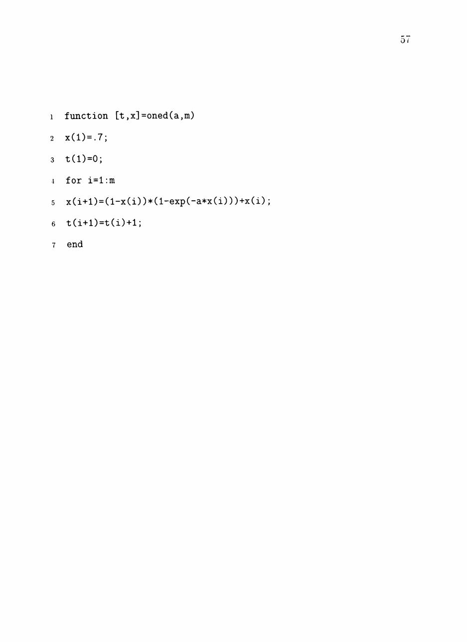
1 function [t,x]=oned(a,m)
2 x ( l ) = . 7 ;
3 t ( l )=0;
4 for i=l :m
5 x(i+l)=(l-x(i))*(l-exp(-a*x(i)))+x(i) ;
6 t ( i+ l )= t ( i )+ l ;
7 end

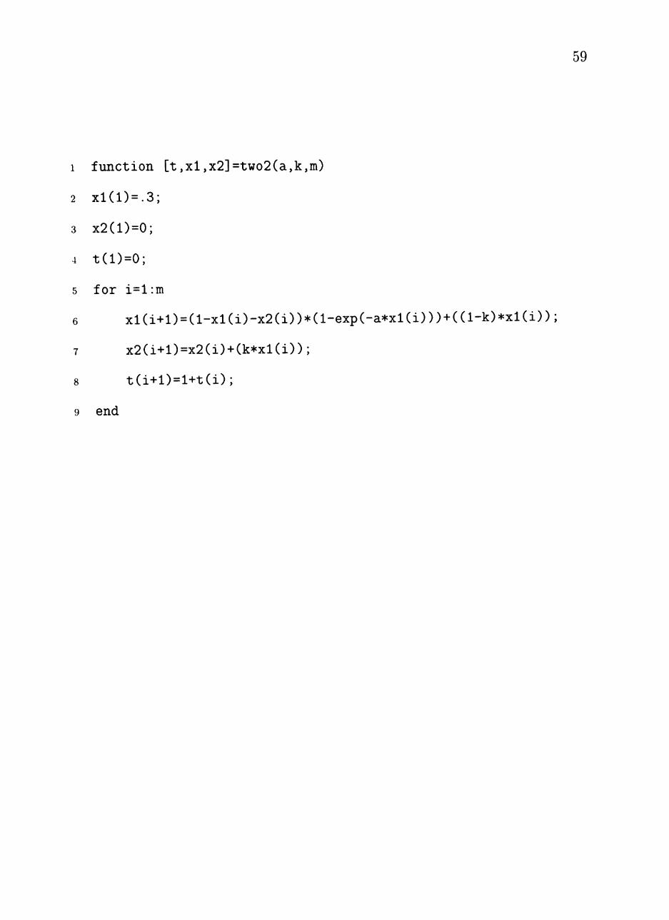
APPENDIX C
SIR MODEL WITH NO VITAL DYNAMICS PROGRAM
58
59
1 function [t,xl,x2]=two2(a,k,m)
2 x l ( l ) = . 3 ;
3 x2(l)=0;
4 t ( l ) = 0 ;
5 fo r i=l :m
6 x l ( i+l )=( l -x l ( i ) -x2( i ) )*( l -exp(-a*xl ( i ) ) )+(( l -k)*xl ( i ) ) ;
7 x2(i+l)=x2(i)+(k*xl(i));
8 t ( i+ l )= l+ t ( i ) ;
9 end
APPENDIX D
SIS MODEL WITH VITAL DYNAMICS PROGRAM
60

61
1 function [t,x]=twod(a,k,m)
2 x ( l ) = . 7 ;
3 t ( l )=0;
4 for i=l:ni
5 x(i+l)= ( l -x( i ) )*( l -exp(-a*x(i ) ) )+(( l -k)*x(i ) ) ;
6 t ( i+ l )= t ( i )+ l ;
7 end
APPENDIX E
SIRS MODEL WITH VITAL DYNAMICS PROGRAM
62

63
1 function [ t ,x l ,x2]=f ived(a ,k , l , s ,m)
2 x l ( l ) = . 3 ;
3 x2(l)=0;
4 t ( l ) = 0 ;
5 for i=l:in
6 x l ( i + l ) = ( l - x l ( i ) - x 2 ( i ) ) * ( l - e x p ( - a * x l ( i ) ) ) + ( ( l - k - l ) * x l ( i ) ) ;
7 x2 ( i+ l )= (x2 ( i )* ( l - s - l ) )+ (k*x l ( i ) ) ;
8 t ( i + l ) = l + t ( i ) ;
9 end

APPENDIX F
SIR^R^S MODEL WITH VITAL DYNAMICS PROGRAM
64

65
1 function [t ,xl,x2,x3]=threed(a,k,s,j ,m)
2 x l ( l ) = . l ;
3 x 2 ( l ) = . 2 5 ;
4 x3(l)=.35;
5 t ( l )=0;
6 fo r i=l:m
7 xl ( i+l )=( l -x l ( i ) -x2( i ) -x3( i ) )*( l -exp(-a*xl( i ) ) ;
8 + ( ( l - k ) * x l ( i ) ) ) ;
9 x2(i+l)=(k*xl(i))+(x2(i)*(l-s));
10 x3(i+l)=(s*x2(i))+((l-j)*x3(i));
11 t(i+l)=l+t(i);
12 e n d

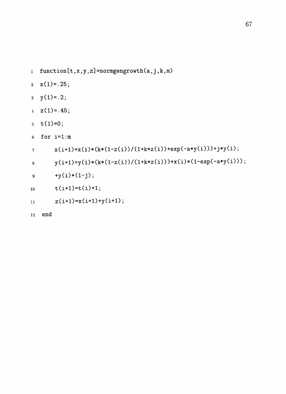
APPENDIX G
SIS MODEL WITH GENERAL GROWTH DYNAMICS PROGRAM
66
67
1 funct ion[t,x,y,z]=normgengrowth(a,j,k,m)
2 x(l)=.25;
3 y(l)=.2;
4 z(l)=.45;
5 t(l)=0;
6 for i=l:m
7 x(i+l)=x(i)*(k*(l-z(i))/(l+k*z(i))+exp(-a*y(i)))+j*y(i);
8 y(i+l)=y(i)*(k*(l-z(i))/(l+k*z(i)))+x(i)*(l-exp(-a*y(i)));
9 +y(i)*(l-j);
10 t(i+l)=t(i)+l;
11 z(i+l)=x(i+l)+y(i+l);
12 end

PERMISSION TO COPY
In presenting this thesis in partial fulfillment of the
requirements for a master's degree at Texas Tech University or
Texas Tech University Health Sciences Center. I agree that the Library
and my major department shall make it freely available for research
purposes. Permission to copy this thesis for scholarly purposes may
be granted by the Director of the Library or my major professor. It
is understood that any copying or publication of this thesis for
financial gain shall not be allowed without my further written
permission and that any user may be liable for copyright infringement.
Agree (Permission is granted.)
Student's Signature Date
Disagree (Permission is not granted.)
Student's Signature Date